Embed Size (px)
Citation preview
Summarization and classification of wearable camera streams by learning the
distributions over deep features of out-of-sample image sequences
Alessandro Perina
WDG Core Data - Microsoft Corp.
Sadegh Mohammadi
PAVIS Dept. - Italian Institute of Technology
Nebojsa Jojic
Microsoft Research
Vittorio Murino
PAVIS Dept. - Italian Institute of Technology
and University of Verona
Abstract
A popular approach to training classifiers of new image classes
is to use lower levels of a pre-trained feed-forward neural network
and retrain only the top. Thus, most layers simply serve as highly
nonlinear feature extractors. While these features were found use-
ful for classifying a variety of scenes and objects, previous work
also demonstrated unusual levels of sensitivity to the input espe-
cially for images which are veering too far away from the training
distribution. This can lead to surprising results as an impercepti-
ble change in an image can be enough to completely change the
predicted class. This occurs in particular in applications involving
personal data, typically acquired with wearable cameras (e.g., vi-
sual lifelogs), where the problem is also made more complex by the
dearth of new labeled training data that make supervised learning
with deep models difficult. To alleviate these problems, in this pa-
per we propose a new generative model that captures the feature
distribution in new data. Its latent space then becomes more rep-
resentative of the new data, while still retaining the generalization
properties. In particular, we use constrained Markov walks over a
counting grid for modeling image sequences, which not only yield
good latent representations, but allow for excellent classification
with only a handful of labeled training examples of the new scenes
or objects, a scenario typical in lifelogging applications.
1. Introduction
Visual lifelogging refers to the process of seamessly collecting
visual data by means of wearable cameras, and it is intended to
capture the bearer’s visual experience of over long and continu-
ous periods of time [4]. Visual lifelogs are recorded for personal
consumption or just for fun, although they also offered valuable
streams in medical applications, such as aids in elderly memory
lacks [6], or dietary analysis [21].
Lifelogging cameras have recently become available to the
consumer market: examples are YoCam, Autographer, Narrative,
EE CaptureCam. Unlike traditional cameras, these devices are
characterized by a passive record-it-all approach and by a low tem-
poral resolution (LTH), automatically shooting a photo every 10-
30 seconds.A popular approach to training classifiers of new image
classes is to use lower levels of a pre-trained feed-forward neural
network and retrain only the top. Thus, most layers simply serve
as highly nonlinear feature extractors. While these features were
found useful for classifying a variety of scenes and objects, pre-
vious work also demonstrated unusual levels of sensitivity to the
input especially for images which are veering too far away from
the training distribution. This can lead to surprising results as an
imperceptible change in an image can be enough to completely
change the predicted class. This occurs in particular in applica-
tions involving personal data, typically acquired with wearable
cameras (e.g., visual lifelogs), where the problem is also made
more complex by the dearth of new labeled training data that make
supervised learning with deep models difficult. To alleviate these
problems, in this paper we propose a new generative model that
captures the feature distribution in new data. Its latent space then
becomes more representative of the new data, while still retain-
ing the generalization properties. In particular, we use constrained
Markov walks over a counting grid for modeling image sequences,
which not only yield good latent representations, but allow for ex-
cellent classification with only a handful of labeled training exam-
ples of the new scenes or objects, a scenario typical in lifelogging
applications.
With increasing amounts of visual data collected, a manual
use of visual lifelogs to infer meaningful knowledge concerning
people’s lives becomes a tedious task. This has opened up a new
line of research in computer vision that tackle lifelogging, includ-
ing automated life story creation [18], summarization [15], action
or location recognition [24], or understanding social interactions
[8, 1].
Despite of significant work in this area, automated visual anal-
ysis of such collections of personal data still remains an open prob-
lem mainly because of i) challenging imaging conditions such as
blurring and motion artifacts due to the loose attachment of the
camera to clothes, ii) abrupt lighting variations, severe occlusions
or presence of non-informative frames due to the non-intentional
14326
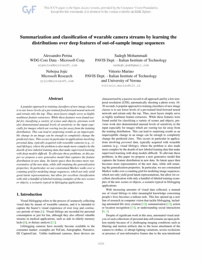
Figure 1. An embedding provided by constrained Markov walks on All-I-Have-Seen (AIHS) [15] dataset. Contiguous regions are seen as
capturing consistent scenes. For instance, the highlighted region belongs to images taken inside the office of the lifelogger.
nature of the image capturing, and iii) very limited amount of la-
beled data to solve a problem with supervised learning1. These
three problems cause major problems for the most powerful clas-
sification frameworks, such as the Convolutional Neural Networks
(CNN), which are typically trained on very large amount of la-
beled, artifact-free images captured in an intentional manner.
One approach to resolving these issues is to pre-train a CNN
on sufficient amount of out out-of-sample, but related and labeled
training data (such as the MIT-Places database, trained with 8 mil-
lion images in 365 scene categories [31]), and transfer its image
representation to a given task. Particularly, one or multiple layers
of the CNN activations may serve as highly non-linear feature ex-
tractors, and new classifiers for new data can be trained on these
features [27]. Although this approach was found useful in clas-
sification of a wide variety of scenes and objects [27, 7], it also
demonstrated unusual levels of sensitivity to the input distribution.
Indeed, extracted deep features can lead to surprising results on in-
1Typically, only the bearer of the camera can provide labels for the
things they care about, making crowdsourcing impractical.
put images which are veering too far away from the training distri-
bution. For instance, two recent studies have shown that not only
an imperceptible change in an image can be enough to completely
change the predicted class [11], but also that CNNs can easily be
fooled with images humans do not consider meaningful, whereas
deep networks classify them with very high confidence as exam-
ples of the known classes [20]. This can lead to major problems in
visual lifelog applications, where video data recorded in the daily
life differs substantially from the training data distribution. Most
importantly, additional classifier training on extracted features still
requires more labeled data than can be expected to be available in
practice, where the users will likely find it tedious to label more
than a couple of images for each class of interest, lest they decide
to limit their interest to a small number of classes.
To mitigate these problems, this paper advocates the use of a
generative model to capture the distribution over the deep features
calculated using the pre-trained model but on the new data. By
fitting the generative model in an unsupervised fashion, the cor-
related changes that affect feature extractors when they move on
to the new domain are captured and explained away without the
4327
need for labeled data. The latent structure of the model then be-
comes the grounds for reasoning about the images in a manner
less affected by the transfer. Additionally, generative models can
be made more interpretable than neural networks’ activations, al-
lowing users to engage with the data in more effective ways than
by simply labeling examples.
In particular, the latent space of the model here corresponds to
the positions in a 2-D grid as illustrated in Figure 1 where we show
a representative image in each location. In this embedding space,
similar images, even when the CNN may assign them to different
classes, tend to map to nearby locations. The directions of varia-
tion across the space tend to follow the recognizable patterns from
the data, such as camera direction, even when images are captured
at a very low temporal resolution of one image per minute. For ex-
ample, a number of images captured inside an office are mapped
to the contiguous area outlined in the embedding. This model is
quite versatile, as it can be used as an unsupervised learning tool,
e.g. for clustering or summarizing the data without use of labels,
but it can also be used to build classifiers with ultra-low numbers
of labeled images.
Contributions. First, we show that the parameterization of
the counting grids (CG) [23], follows the typical neural network
parametrization, thus justifying their use as the final layer in a deep
architecture for a hybrid forward-backward model, where feature
extractors applied in forward manner are expected to follow a dis-
tribution of a generative model with grid position as a latent vari-
able. Counting grids are generative models that embed discrete
data onto a 2-D discrete torus. They are robust in presence of
data scarcity, and have been previously used for lifelogging-related
tasks like image retrieval [10] or location recognition [22, 24].
Second, we extended the counting grid model by enforcing the
temporal consistency of the mappings using constrained Markov
walks. We partition the visual stream into contiguous snippets of
frames and jointly embed the frames of each snippet by means
of a constrained version of the forward-backward algorithm [25].
This allows us to find better local minima of frame embedding into
CG where having multiple distant areas corresponding to the same
type of images is avoided. A further benefit is an improved robust-
ness to non-informative frames, which are mapped into ”garbage
areas” by the regular counting grid, and consume precious real-
estate on the grid. With constrained Markov walks each frame
is mapped jointly with its neighbors and because we expect that
at least 50% of the frames in a snippet are informative, they will
guide the mapping of the whole snippet disallowing creation of
separate areas with overexposed or occluded images. Finally, en-
forcing temporal consistency maps the locations which are close in
the real word into locations that are also close on the grid, making
the embedding more suitable for browsing or personal consump-
tion.
Finally, we prove that inference can be carried out in linear
time by adapting the forward-backward procedure (which is usu-
ally quadratic) to exploit the counting grid geometry for particular
shapes of the Markov constraint, from boxes to Gaussians.
In the experiments, we consider three recent types of visual
streams acquired with wearable cameras [28, 15, 17], and we ex-
ploited the mappings in the embedding to asses the similarity of
images rather than the direct comparison of feature vectors. Our
results unquestionably show that that the embedding produced by
this new model allows classification with ultra-low number of la-
beled examples better than standard supervised layers (e.g., Soft-
max), and also compares favorably to the unsupervised embed-
dings provided by autoencoders [2], t-sne [29], and regular count-
ing grids. This functionality, which next to low power consump-
tion, is one of the most needed precursors to adoption of wearable
cameras and their applications.
The rest of the paper is organized as follows. In Section 2,
the literature close to the proposed approach is addressed. Section
3 details the proposed variation of the counting grid generative
model, showing how it is able to properly organise the latent space.
Extensive experimental results are reported in Section 4, together
with comparative analyses. Section 5 draws the conclusions and
sketches future perspectives.
2. Constrained Markov walks over a counting
grid
In this section we first review the basic counting grid models
[23], then we turn to present our contributions: i) we justify count-
ing grids as generative layer in deep architectures, ii) we extend the
counting grid by constraining the walks on its embedding, calling
the resulting model CGcw and finally iii) we show how inference
in this new model can be carried out in linear time.
The Counting Grid Suppose that each image frame xt is
represented by a set of non-negative feature intensities, xt =
{ctz}Zz=1. Each frame is associated with a discrete location ℓt
on a 2-dimensional toroidal grid2E = Er × Ec. The location
ℓ = (ℓr, ℓc) is a latent variable that defines the mapping on the
grid thus the distribution over possible feature observations for a
single frame t as:
p(xt|ℓt) =∏
z
hctzℓ,z, (1)
Where hℓ,z is a distribution over features z associated with loca-
tion ℓ, thus∑
zhℓ,z = 1. A feature intensity cz is thus treated
as a count, as if there was a discrete detector for feature z that
was tripped cz times, and the feature probabilities hℓ,z form a nor-
malized expected histogram of counts. For example, the z − thdetector could be associated with a particular image pixel or, as is
the case in our experiments, it can correspond to the output of a
particular neuron in a neural network.
The large number of distributions hℓ,z are constrained by the
underlying set of sparse distributions πi,z and by the choice of
an averaging window W = Wr × Wc which is typically much
smaller than the grid, in formulae the relationship between h and
π is
hℓ,z =1
|W|
∑
i∈Wℓ
πi,z (2)
being |W| the area of the averaging window |W| = Wr ·Wc (we
will use the same notation for the grid’s estate) and Wℓ the par-
ticular window that starts at location ℓ and expands in the lower
2On a toroidal grid, the location (0,0) is a unit distance away from both
(0,1) and (0,63), and two units of distance away from both (0,2) and (0,62),
etc; or in other words, the locations are considered in a (mod 64) sense
- See Figure 2
4328
0,0 0,1
1,0
3,3
...
...
0,630,9...
...
...
...
...
...
...
...
...
...
...
... ... ... ... ... ... ... ... ... ... ...
0,0
6,6
3,0
2,0
0,4
3,4
...
0,1
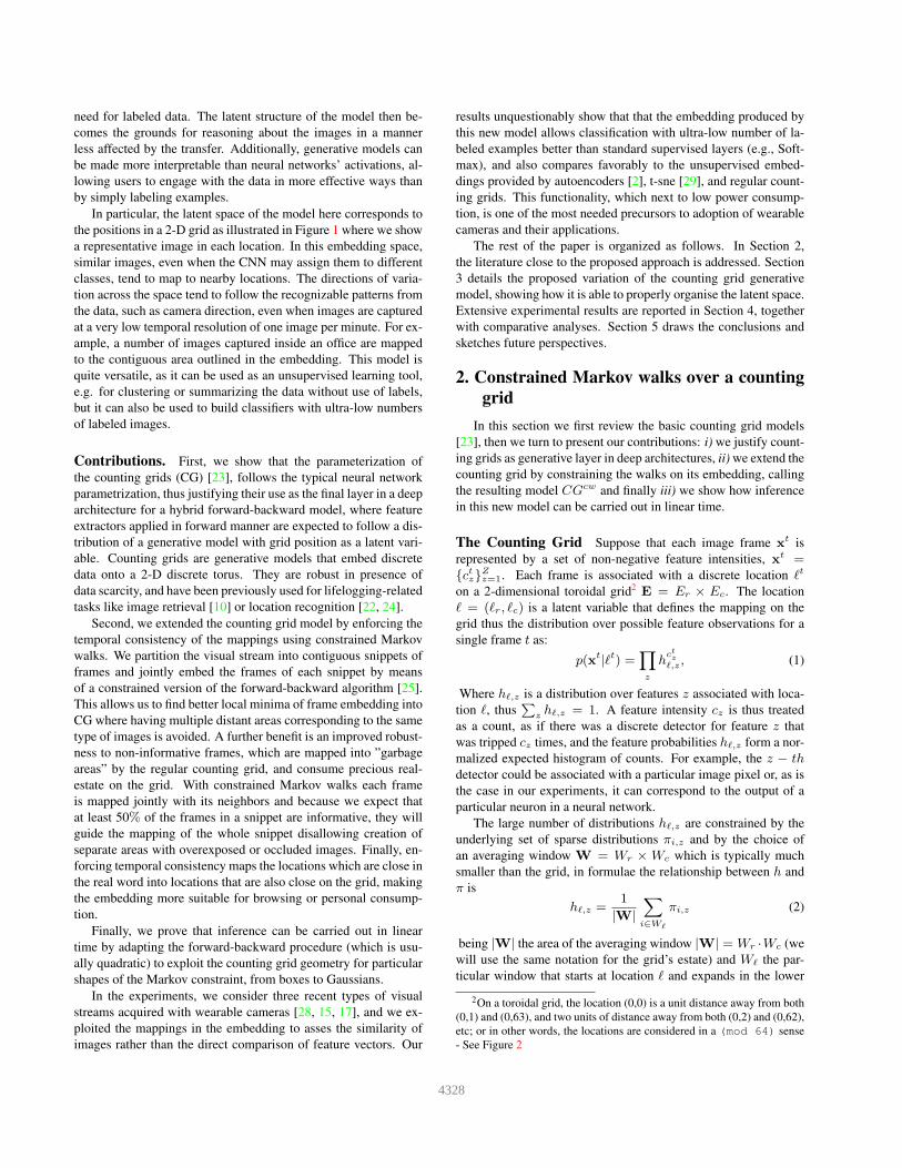
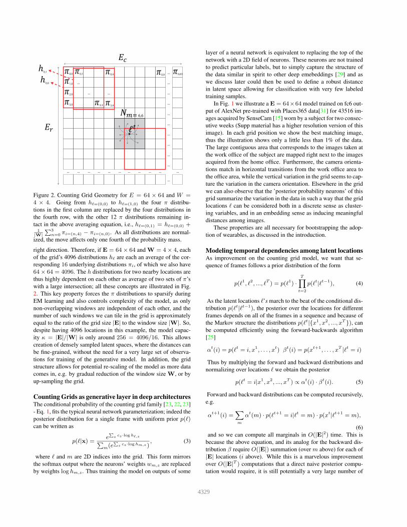
Figure 2. Counting Grid Geometry for E = 64 × 64 and W =4 × 4. Going from hℓ=(0,0) to hℓ=(1,0) the four π distribu-
tions in the first column are replaced by the four distributions in
the fourth row, with the other 12 π distributions remaining in-
tact in the above averaging equation, i.e., hℓ=(0,1) = hℓ=(0,0) +1
|W|
∑3n=0 πi=(n,4) − πi=(n,0). As all distributions are normal-
ized, the move affects only one fourth of the probability mass.
right direction. Therefore, if E = 64× 64 and W = 4× 4, each
of the grid’s 4096 distributions hℓ are each an average of the cor-
responding 16 underlying distributions πi, of which we also have
64× 64 = 4096. The h distributions for two nearby locations are
thus highly dependent on each other as average of two sets of π’s
with a large intersection; all these concepts are illustrated in Fig.
2. This key property forces the π distributions to sparsify during
EM learning and also controls complexity of the model, as only
non-overlapping windows are independent of each other, and the
number of such windows we can tile in the grid is approximately
equal to the ratio of the grid size |E| to the window size |W|. So,
despite having 4096 locations in this example, the model capac-
ity κ = |E|/|W| is only around 256 = 4096/16. This allows
creation of densely sampled latent spaces, where the distances can
be fine-grained, without the need for a very large set of observa-
tions for training of the generative model. In addition, the grid
structure allows for potential re-scaling of the model as more data
comes in, e.g. by gradual reduction of the window size W, or by
up-sampling the grid.
Counting Grids as generative layer in deep architecturesThe conditional probability of the counting grid family [23, 22, 23]
- Eq. 1, fits the typical neural network parameterization; indeed the
posterior distribution for a single frame with uniform prior p(ℓ)can be written as
p(ℓ|x) =e∑
z cz ·log hℓ,z
∑
m(e
∑z cz ·log hm,z )
, (3)
where ℓ and m are 2D indices into the grid. This form mirrors
the softmax output where the neurons’ weights wm,z are replaced
by weights log hm,z . Thus training the model on outputs of some
layer of a neural network is equivalent to replacing the top of the
network with a 2D field of neurons. These neurons are not trained
to predict particular labels, but to simply capture the structure of
the data similar in spirit to other deep emebeddings [29] and as
we discuss later could then be used to define a robust distance
in latent space allowing for classification with very few labeled
training samples.
In Fig. 1 we illustrate a E = 64×64 model trained on fc6 out-
put of AlexNet pre-trained with Places365 data[31] for 43516 im-
ages acquired by SenseCam [15] worn by a subject for two consec-
utive weeks (Supp material has a higher resolution version of this
image). In each grid position we show the best matching image,
thus the illustration shows only a little less than 1% of the data.
The large contiguous area that corresponds to the images taken at
the work office of the subject are mapped right next to the images
acquired from the home office. Furthermore, the camera orienta-
tions match in horizontal transitions from the work office area to
the office area, while the vertical variation in the grid seems to cap-
ture the variation in the camera orientation. Elsewhere in the grid
we can also observe that the ’posterior probability neurons’ of this
grid summarize the variation in the data in such a way that the grid
locations ℓ can be considered both in a discrete sense as cluster-
ing variables, and in an embedding sense as inducing meaningful
distances among images.
These properties are all necessary for bootstrapping the adop-
tion of wearables, as discussed in the introduction.
Modeling temporal dependencies among latent locationsAs improvement on the counting grid model, we want that se-
quence of frames follows a prior distribution of the form
p(ℓ1, ℓ2, ..., ℓT ) = p(ℓ1) ·
T∏
t=2
p(ℓt|ℓt−1), (4)
As the latent locations ℓ’s march to the beat of the conditional dis-
tribution p(ℓt|ℓt−1), the posterior over the locations for different
frames depends on all of the frames in a sequence and because of
the Markov structure the distributions p(ℓt|{x1, x2, ..., xT }), can
be computed efficiently using the forward-backwards algorithm
[25]
αt(i) = p(ℓt = i, x1, . . . , xt) βt(i) = p(xt+1, . . . , xT |ℓt = i)
Thus by multiplying the forward and backward distributions and
normalizing over locations ℓ we obtain the posterior
p(ℓt = i|x1, x2, ..., xT ) ∝ αt(i) · βt(i). (5)
Forward and backward distributions can be computed recursively,
e.g.
αt+1(i) =∑
m
αt(m) · p(ℓt+1 = i|ℓt = m) · p(xt|ℓt+1 = m),
(6)
and so we can compute all marginals in O(|E|2) time. This is
because the above equation, and its analog for the backward dis-
tribution β require O(|E|) summation (over m above) for each of
|E| locations (i above). While this is a marvelous improvement
over O(|E|T ) computations that a direct naive posterior compu-
tation would require, it is still potentially a very large number of
4329
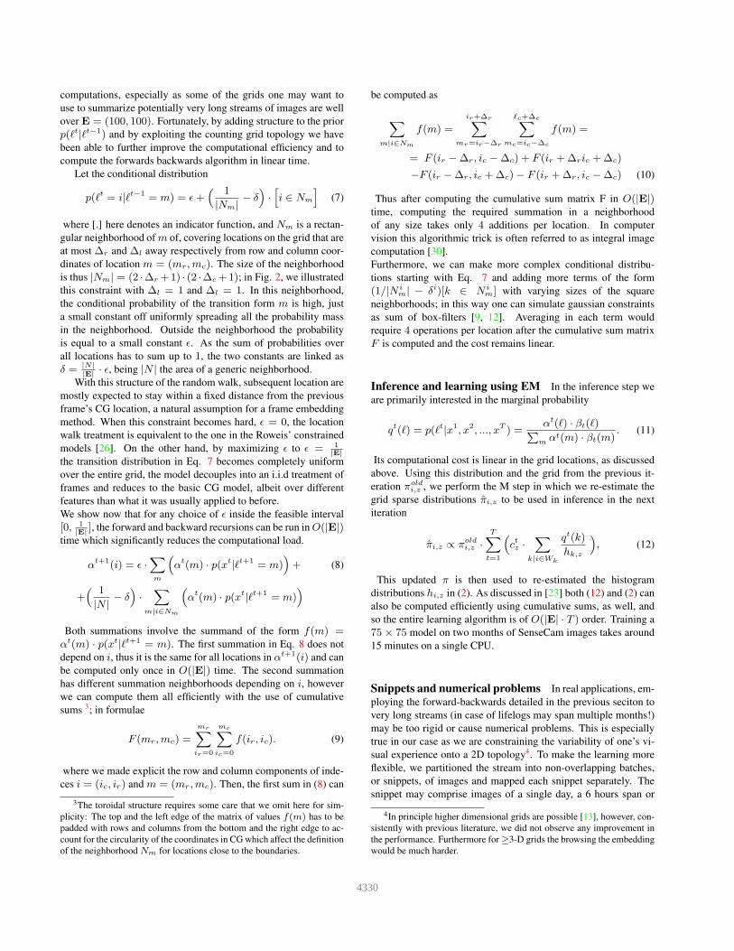
computations, especially as some of the grids one may want to
use to summarize potentially very long streams of images are well
over E = (100, 100). Fortunately, by adding structure to the prior
p(ℓt|ℓt−1) and by exploiting the counting grid topology we have
been able to further improve the computational efficiency and to
compute the forwards backwards algorithm in linear time.
Let the conditional distribution
p(ℓt = i|ℓt−1 = m) = ǫ+( 1
|Nm|− δ
)
·[
i ∈ Nm
]
(7)
where [.] here denotes an indicator function, and Nm is a rectan-
gular neighborhood of m of, covering locations on the grid that are
at most ∆r and ∆l away respectively from row and column coor-
dinates of location m = (mr,mc). The size of the neighborhood
is thus |Nm| = (2 ·∆r +1) · (2 ·∆c+1); in Fig. 2, we illustrated
this constraint with ∆l = 1 and ∆l = 1. In this neighborhood,
the conditional probability of the transition form m is high, just
a small constant off uniformly spreading all the probability mass
in the neighborhood. Outside the neighborhood the probability
is equal to a small constant ǫ. As the sum of probabilities over
all locations has to sum up to 1, the two constants are linked as
δ = |N||E|
· ǫ, being |N | the area of a generic neighborhood.
With this structure of the random walk, subsequent location are
mostly expected to stay within a fixed distance from the previous
frame’s CG location, a natural assumption for a frame embedding
method. When this constraint becomes hard, ǫ = 0, the location
walk treatment is equivalent to the one in the Roweis’ constrained
models [26]. On the other hand, by maximizing ǫ to ǫ = 1|E|
the transition distribution in Eq. 7 becomes completely uniform
over the entire grid, the model decouples into an i.i.d treatment of
frames and reduces to the basic CG model, albeit over different
features than what it was usually applied to before.
We show now that for any choice of ǫ inside the feasible interval
[0, 1|E|
], the forward and backward recursions can be run in O(|E|)time which significantly reduces the computational load.
αt+1(i) = ǫ ·∑
m
(
αt(m) · p(xt|ℓt+1 = m))
+ (8)
+( 1
|N |− δ
)
·∑
m|i∈Nm
(
αt(m) · p(xt|ℓt+1 = m))
Both summations involve the summand of the form f(m) =αt(m) · p(xt|ℓt+1 = m). The first summation in Eq. 8 does not
depend on i, thus it is the same for all locations in αt+1(i) and can
be computed only once in O(|E|) time. The second summation
has different summation neighborhoods depending on i, however
we can compute them all efficiently with the use of cumulative
sums 3; in formulae
F (mr,mc) =
mr∑
ir=0
mc∑
ic=0
f(ir, ic). (9)
where we made explicit the row and column components of inde-
ces i = (ic, ir) and m = (mr,mc). Then, the first sum in (8) can
3The toroidal structure requires some care that we omit here for sim-
plicity: The top and the left edge of the matrix of values f(m) has to be
padded with rows and columns from the bottom and the right edge to ac-
count for the circularity of the coordinates in CG which affect the definition
of the neighborhood Nm for locations close to the boundaries.
be computed as
∑
m|i∈Nm
f(m) =
ir+∆r∑
mr=ir−∆r
ℓc+∆c∑
mc=ic−∆c
f(m) =
= F (ir −∆r, ic −∆c) + F (ir +∆ric +∆c)
−F (ir −∆r, ic +∆c)− F (ir +∆r, ic −∆c) (10)
Thus after computing the cumulative sum matrix F in O(|E|)time, computing the required summation in a neighborhood
of any size takes only 4 additions per location. In computer
vision this algorithmic trick is often referred to as integral image
computation [30].
Furthermore, we can make more complex conditional distribu-
tions starting with Eq. 7 and adding more terms of the form
(1/|N im| − δi)[k ∈ N i
m] with varying sizes of the square
neighborhoods; in this way one can simulate gaussian constraints
as sum of box-filters [9, 12]. Averaging in each term would
require 4 operations per location after the cumulative sum matrix
F is computed and the cost remains linear.
Inference and learning using EM In the inference step we
are primarily interested in the marginal probability
qt(ℓ) = p(ℓt|x1, x2, ..., xT ) =αt(ℓ) · βt(ℓ)
∑
mαt(m) · βt(m)
. (11)
Its computational cost is linear in the grid locations, as discussed
above. Using this distribution and the grid from the previous it-
eration πoldi,z , we perform the M step in which we re-estimate the
grid sparse distributions πi,z to be used in inference in the next
iteration
πi,z ∝ πoldi,z ·
T∑
t=1
(
ctz ·∑
k|i∈Wk
qt(k)
hk,z
)
, (12)
This updated π is then used to re-estimated the histogram
distributions hi,z in (2). As discussed in [23] both (12) and (2) can
also be computed efficiently using cumulative sums, as well, and
so the entire learning algorithm is of O(|E| · T ) order. Training a
75× 75 model on two months of SenseCam images takes around
15 minutes on a single CPU.
Snippets and numerical problems In real applications, em-
ploying the forward-backwards detailed in the previous seciton to
very long streams (in case of lifelogs may span multiple months!)
may be too rigid or cause numerical problems. This is especially
true in our case as we are constraining the variability of one’s vi-
sual experience onto a 2D topology4. To make the learning more
flexible, we partitioned the stream into non-overlapping batches,
or snippets, of images and mapped each snippet separately. The
snippet may comprise images of a single day, a 6 hours span or
4In principle higher dimensional grids are possible [13], however, con-
sistently with previous literature, we did not observe any improvement in
the performance. Furthermore for ≥3-D grids the browsing the embedding
would be much harder.
4330

a random number of consecutive images (depends on the appli-
cation and the characteristics of the stream). Finally, in the case
the forward-backwards procedure still resulted in numerical un-
derflow one can employ the same technique used to learn stel-
eptiomes [15] or further reduce the batch size.
3. Experiments
We tested our proposed method on three challenging and re-
cent datasets: Google Glass (GG) dataset [17], All-I-Have-Seen
(AIHS) SenseCam dataset [22], and Multimodal Egocentric Ac-
tivity (MEA) dataset [28].
In all experiments, we used the output of the fc6 layer ex-
tracted from the pre-trained AlexNet [16] as the frame-level de-
scriptor. (We also tested other NN layers, but, consistently with
previous work [10] found fc6 to work best.) We used the reg-
ular counting grids and our proposed extension CGcw to learn
the distributions over these deep features. We varied grid E and
window W size of the counting grid’d discrete 2-Dimensional
space as E ∈ {50× 50, 60× 60, 70× 70, 80× 80} and W ∈{3× 3, 5× 5, 7× 7}, respectively. As for the neighborhood Nm,
we tested box constraints with ∆r,∆c ∈ {1, 2, 3}, finding these
parameters to play a crucial role in the performance of model.
We partitioned the video streams into snippets of Miter sam-
pling at each iteration of the EM algorithm a Poisson distribution
Miter ∼ Poisson(λ = 10). Finally, to assign labels at test time,
we used a Nearest Neighbor (NN) classifier and Euclidean dis-
tance on a torus. Throughout all the experiments, we compared
our method with the following baseline methods
1. fc6+NN: As first baseline, we used fc6 deep feature with
4096 dimensions extracted from AlexNet [16] and NN with
Euclidean distance.
2. Softmax: As second baseline, we plugged the usual softmax
layer over fc6 deep features.
3. t-Distributed Stochastic Neighbor embedding - tSNE [29]:
Instead of counting grids, tSNE was used to project deep
features into 2-D embedding space, and to assign labels at
test time we used nearest neighbor classifier with Euclidean
distance.
4. Two-layers deep autoencoders - AE [2]: In this case, embed-
ding of all images in a stream was done with AE. We varied
the first hidden and the second hidden units in the range of
{50, 100, 200, 300} and {2, 50, 100, 200}.
3.1. The effect of the constrained walk: AIHSDataset
The AIHS dataset contains 43522 images captured from 45 lo-
cations (e.g., office, dinning room, etc.). Methods were compared
in the standard leave-one-out testing protocol. In this test, we set
the constant ǫ = 10−6 (Eq. 7) for the first X% iterations of the
EM algorithm (we used a fixed number of iteration), after which
for the rest of the training (till convergence) the parameter is re-set
to ǫ = 1|E|
turning the model into the basic CG model. Figure 3
shows the accuracy on the 45-class classification task versus the
percentage of the iterations spent learning with the constrained
walk in the early phase for three different sizes of the constraint
Nm.
Figure 3. The effect of varying constraint neighborhood on the
quality of embedding of AIHS dataset.
Figure 4. Visual Comparison of CGcw with tSNE. First column
shows the whole embedding spaces of CGcw and tSNE [29].
Green regions are sections of the area where office images tend
to map. Second column shows the zoomed in green regions. The
red regions indicate location where tSNE [29] has non-office im-
ages mingled with the office images.
We found that even enforcing the temporal consistency for only
10% of the training time dramatically improved the classification
accuracy. This means that the trained grids are also reaching better
local minima for the unconstrained CG model compared to what
the basic EM algorithm can achieve. We should also note that
first point in the graph at 65% attests that just switching from
pixel intensities to fc6 features did half the work in improving
over the previous state of the art of around 60.2% [22], which
was also based on CGs. The other half of the total improvement is
achieved by learning with constrained walks. Finally, consistently
with previous literature on counting grids, the grid-window ratio
did not play a key role here and we only observed variations of
only around 3% accuracy across the values we considered.
4331
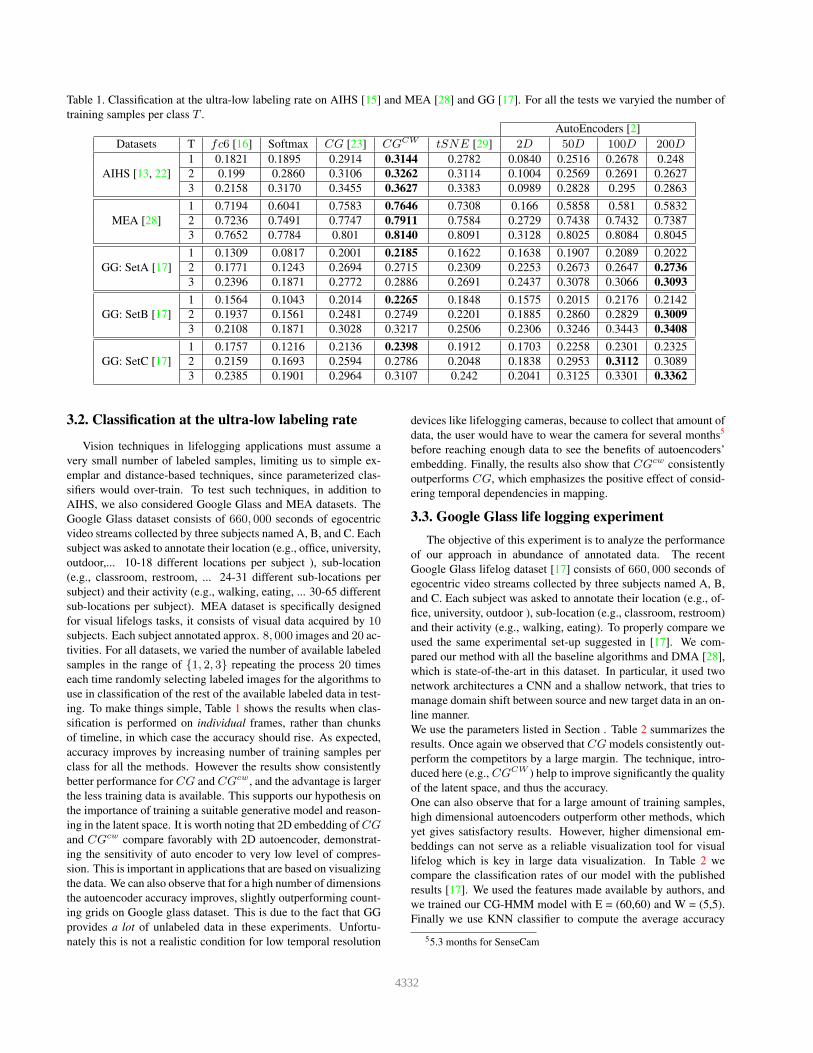
Table 1. Classification at the ultra-low labeling rate on AIHS [15] and MEA [28] and GG [17]. For all the tests we varyied the number of
training samples per class T .
AutoEncoders [2]
Datasets T fc6 [16] Softmax CG [23] CGCW tSNE [29] 2D 50D 100D 200D
AIHS [13, 22]
1 0.1821 0.1895 0.2914 0.3144 0.2782 0.0840 0.2516 0.2678 0.248
2 0.199 0.2860 0.3106 0.3262 0.3114 0.1004 0.2569 0.2691 0.2627
3 0.2158 0.3170 0.3455 0.3627 0.3383 0.0989 0.2828 0.295 0.2863
MEA [28]
1 0.7194 0.6041 0.7583 0.7646 0.7308 0.166 0.5858 0.581 0.5832
2 0.7236 0.7491 0.7747 0.7911 0.7584 0.2729 0.7438 0.7432 0.7387
3 0.7652 0.7784 0.801 0.8140 0.8091 0.3128 0.8025 0.8084 0.8045
GG: SetA [17]
1 0.1309 0.0817 0.2001 0.2185 0.1622 0.1638 0.1907 0.2089 0.2022
2 0.1771 0.1243 0.2694 0.2715 0.2309 0.2253 0.2673 0.2647 0.2736
3 0.2396 0.1871 0.2772 0.2886 0.2691 0.2437 0.3078 0.3066 0.3093
GG: SetB [17]
1 0.1564 0.1043 0.2014 0.2265 0.1848 0.1575 0.2015 0.2176 0.2142
2 0.1937 0.1561 0.2481 0.2749 0.2201 0.1885 0.2860 0.2829 0.3009
3 0.2108 0.1871 0.3028 0.3217 0.2506 0.2306 0.3246 0.3443 0.3408
GG: SetC [17]
1 0.1757 0.1216 0.2136 0.2398 0.1912 0.1703 0.2258 0.2301 0.2325
2 0.2159 0.1693 0.2594 0.2786 0.2048 0.1838 0.2953 0.3112 0.3089
3 0.2385 0.1901 0.2964 0.3107 0.242 0.2041 0.3125 0.3301 0.3362
3.2. Classification at the ultralow labeling rate
Vision techniques in lifelogging applications must assume a
very small number of labeled samples, limiting us to simple ex-
emplar and distance-based techniques, since parameterized clas-
sifiers would over-train. To test such techniques, in addition to
AIHS, we also considered Google Glass and MEA datasets. The
Google Glass dataset consists of 660, 000 seconds of egocentric
video streams collected by three subjects named A, B, and C. Each
subject was asked to annotate their location (e.g., office, university,
outdoor,... 10-18 different locations per subject ), sub-location
(e.g., classroom, restroom, ... 24-31 different sub-locations per
subject) and their activity (e.g., walking, eating, ... 30-65 different
sub-locations per subject). MEA dataset is specifically designed
for visual lifelogs tasks, it consists of visual data acquired by 10subjects. Each subject annotated approx. 8, 000 images and 20 ac-
tivities. For all datasets, we varied the number of available labeled
samples in the range of {1, 2, 3} repeating the process 20 times
each time randomly selecting labeled images for the algorithms to
use in classification of the rest of the available labeled data in test-
ing. To make things simple, Table 1 shows the results when clas-
sification is performed on individual frames, rather than chunks
of timeline, in which case the accuracy should rise. As expected,
accuracy improves by increasing number of training samples per
class for all the methods. However the results show consistently
better performance for CG and CGcw, and the advantage is larger
the less training data is available. This supports our hypothesis on
the importance of training a suitable generative model and reason-
ing in the latent space. It is worth noting that 2D embedding of CGand CGcw compare favorably with 2D autoencoder, demonstrat-
ing the sensitivity of auto encoder to very low level of compres-
sion. This is important in applications that are based on visualizing
the data. We can also observe that for a high number of dimensions
the autoencoder accuracy improves, slightly outperforming count-
ing grids on Google glass dataset. This is due to the fact that GG
provides a lot of unlabeled data in these experiments. Unfortu-
nately this is not a realistic condition for low temporal resolution
devices like lifelogging cameras, because to collect that amount of
data, the user would have to wear the camera for several months5
before reaching enough data to see the benefits of autoencoders’
embedding. Finally, the results also show that CGcw consistently
outperforms CG, which emphasizes the positive effect of consid-
ering temporal dependencies in mapping.
3.3. Google Glass life logging experiment
The objective of this experiment is to analyze the performance
of our approach in abundance of annotated data. The recent
Google Glass lifelog dataset [17] consists of 660, 000 seconds of
egocentric video streams collected by three subjects named A, B,
and C. Each subject was asked to annotate their location (e.g., of-
fice, university, outdoor ), sub-location (e.g., classroom, restroom)
and their activity (e.g., walking, eating). To properly compare we
used the same experimental set-up suggested in [17]. We com-
pared our method with all the baseline algorithms and DMA [28],
which is state-of-the-art in this dataset. In particular, it used two
network architectures a CNN and a shallow network, that tries to
manage domain shift between source and new target data in an on-
line manner.
We use the parameters listed in Section . Table 2 summarizes the
results. Once again we observed that CG models consistently out-
perform the competitors by a large margin. The technique, intro-
duced here (e.g., CGCW ) help to improve significantly the quality
of the latent space, and thus the accuracy.
One can also observe that for a large amount of training samples,
high dimensional autoencoders outperform other methods, which
yet gives satisfactory results. However, higher dimensional em-
beddings can not serve as a reliable visualization tool for visual
lifelog which is key in large data visualization. In Table 2 we
compare the classification rates of our model with the published
results [17]. We used the features made available by authors, and
we trained our CG-HMM model with E = (60,60) and W = (5,5).
Finally we use KNN classifier to compute the average accuracy
55.3 months for SenseCam
4332

Table 2. Comparison of average accuracy on Google Glass with
baselines. The final accuracy is computed as the average of three
available annotated levels, namely ”location”, ”sub-location” and
”Activity”, for each subject A, B, and C. 10-folds with 20 times of
repetition using kNN classifier is used for this task.
Subject
Method A B C
CG [14] 0.8256 0.7864 0.7951
CGCW 0.8337 0.8012 0.8103
tSNE [29] 0.7859 0.7052 0.7993
fc6 [16] 0.6117 0.5579 0.732
DMA [28] 0.6702 0.588 0.7757
2D-Autoencoder [2] 0.6096 0.695 0.6193
50D-Autoencoder [2] 0.9308 0.893 0.9254
100D-Autoencoder [2] 0.9384 0.8963 0.9269
200D-Autoencoder [2] 0.9390 0.9037 0.9277
for each subject. The classifier used the distance on the grid be-
tween the locations of the embeddings of the frames (taking grid
wraparound into account). In Table 2 reports summary of our re-
sults we compare the classification rates of our model with the
published results [17]
3.4. Visual Comparison of constrained walk CGwith tSNE Embedding
The embedding plays a central role in visual lifelog applica-
tions such as tracking elderly people health indicators, where we
can track his/her status at every instant of time. In addition, visu-
ally browsable embedding may be unavoidable as a tool in low-
labeling regime as our result show that for 45 classes, with ran-
domly selected 3 images per class to be labeled, the accuracy may
not be higher than 36% early in the life of the device. But with ap-
propriate ways to visualize the data and select areas to label, much
higher levels of accuracy with just as little human labor should
be possible. To this end, we provide a qualitative comparison of
CGcw and tSNE [29] 2D embeddings. Figure 4 shows a compar-
ison of the embedding space [29] which map 43526 images from
the AIHS dataset 6. Neither CGcw nor tSNE exploit annotated
data at the training phase. Different regions of embedding space
tend to belong to different scene categories. For instance, images
taken from office are mapped into a large contiguous area on the
left edge of the CGcw embedding space, while for tSNE all are
mapped to a bottom part of its embedding space. We highlight a
part of office region for both CGcw and tSNE. Although tSNE is
capable of clustering office region, we observe that there are also
irrelevant areas within the tSNE’s office region (highlighted red
regions). For instance, in the top-left corner, an image belonging
to the restaurant category is buried in tSNE’s office area. A closer
inspection reveals the reason for this: there is a chair in front of
the camera bearer which is very similar to the monitor of com-
puter (rectangle black shape) in the first row. We can observe that
lifelogger’s images while working in his/her home with a personal
6 We strongly recommend seeing our supplementary material for fur-
ther analysis and available high resolution embedding space along with a
random walk video
laptop is also mapped into office region. Therefore, we can con-
clude that main feature the tSNE locks onto here, is presence of
computer screen. We should note that high quality mapping in 2D
can allow users to annotate more images with less work by lasso-
ing a whole area as indicated in Fig. 1, in which case the more
advantageous mappings should have fewer noncontiguous areas
belonging to the same category.
4. Conclusions
We presented an original combination of supervised and unsu-
pervised methods for mining personal collections of data acquired
with wearable cameras. Particularly, we extended the counting
grid models to enforce temporal consistency in the latent space
and we used it to model the feature distribution over the responses
of deep networks. Extensive experiments on several benchmarks
demonstrated that the proposed method outperforms a variety or
alternative methods when only a handful of training samples are
available, which is the only realistic scenario in lifelogging ap-
plications. We also showed that the proposed model is able to
produce compelling visualizations space compared to tSNE and
autoencoders, and therefore it has a great potential to serve as a
standard visualization tool for large scale data summarization and
browsing tools.
Finally, it is worth noting that the CGcw model can also be
used as a standalone generative model, i.e not on top of a deep
architecture. For example, we considered the Behave dataset [3]
and the task of abnormal crowd behavior detection. Following the
same evaluation protocol of [5], we learned a model of normal be-
havior, by fitting a CGcw model using bag-of-word descriptors
(See [19] for details). Then, we used the loglikelihood of test
frames to detect abnormal events. Our new model achieved an
AUC of 91.82, outperforming regular counting grids 89.06 and
latent Dirichlet allocation 88.56 with the latter being currently
the most often used technique for learning behaviors from such
data.
References
[1] M. Aghaei, M. Dimiccoli, and P. Radeva. With whom do
I interact? detecting social interactions in egocentric photo-
streams. CoRR, abs/1605.04129, 2016. 1
[2] Y. Bengio et al. Learning deep architectures for ai. Founda-
tions and trends R© in Machine Learning, 2(1):1–127, 2009.
3, 6, 7, 8
[3] S. Blunsden and R. Fisher. The behave video dataset: ground
truthed video for multi-person behavior classification. An-
nals of the BMVA, 4(1-12):4, 2010. 8
[4] M. Bolanos, M. Dimiccoli, and P. Radeva. Toward story-
telling from visual lifelogging: An overview. IEEE Trans.
Human-Machine Systems, 47(1):77–90, 2017. 1
[5] X. Cui, Q. Liu, M. Gao, and D. N. Metaxas. Abnormal detec-
tion using interaction energy potentials. In Computer Vision
and Pattern Recognition (CVPR), 2011 IEEE Conference on,
pages 3161–3167. IEEE, 2011. 8
[6] A. R. Doherty, K. Pauly-Takacs, N. Caprani, C. Gurrin, C. J.
Moulin, N. E. O’Connor, and A. F. Smeaton. Experiences
of aiding autobiographical memory using the sensecam.
Human–Computer Interaction, 27(1-2):151–174, 2012. 1
4333
[7] J. Donahue, Y. Jia, O. Vinyals, J. Hoffman, N. Zhang,
E. Tzeng, and T. Darrell. Decaf: A deep convolutional ac-
tivation feature for generic visual recognition. In Icml, vol-
ume 32, pages 647–655, 2014. 2
[8] A. Fathi, J. K. Hodgins, and J. M. Rehg. Social interac-
tions: A first-person perspective. In CVPR, pages 1226–
1233. IEEE Computer Society, 2012. 1
[9] P. F. Felzenszwalb, D. P. Huttenlocher, and J. M. Kleinberg.
Fast algorithms for large-state-space hmms with applications
to web usage analysis. In S. Thrun, L. Saul, and B. Schlkopf,
editors, Advances in Neural Information Processing Systems
16, page None. MIT Press, Cambridge, MA, 2003. 5
[10] Z. Gao, G. Hua, D. Zhang, J. Xue, and N. Zheng. Counting
grid aggregation for event retrieval and recognition. arXiv
preprint arXiv:1604.01109, 2016. 3, 6
[11] I. J. Goodfellow, J. Shlens, and C. Szegedy. Explain-
ing and harnessing adversarial examples. arXiv preprint
arXiv:1412.6572, 2014. 2
[12] W. M. W. III. Efficient synthesis of gaussian filters by cas-
caded uniform filters. IEEE Trans. Pattern Anal. Mach. In-
tell., 8(2):234–239, 1986. 5
[13] N. Jojic and A. Perina. Multidimensional counting grids:
Inferring word order from disordered bags of words. arXiv
preprint arXiv:1202.3752, 2012. 5, 7
[14] N. Jojic and A. Perina. Multidimensional counting grids:
Inferring word order from disordered bags of words. arXiv
preprint arXiv:1202.3752, 2012. 8
[15] N. Jojic, A. Perina, and V. Murino. Structural epitome: a way
to summarize ones visual experience. In Advances in neural
information processing systems, pages 1027–1035, 2010. 1,
2, 3, 4, 6, 7
[16] A. Krizhevsky, I. Sutskever, and G. E. Hinton. Imagenet
classification with deep convolutional neural networks. In
Advances in neural information processing systems, pages
1097–1105, 2012. 6, 7, 8
[17] S.-W. Lee, C.-Y. Lee, D. H. Kwak, J. Kim, J. Kim, and B.-T.
Zhang. Dual-memory deep learning architectures for life-
long learning of everyday human behaviors. International
Joint Conference on Artificial Intelligence (IJCAI 2016),
2016. 3, 6, 7, 8
[18] Z. Lu and K. Grauman. Story-driven summarization for ego-
centric video. In CVPR, 2013. 1
[19] S. Mohammadi, H. Kiani, A. Perina, and V. Murino. A
comparison of crowd commotion measures from generative
models. In Proceedings of the IEEE Conference on Com-
puter Vision and Pattern Recognition Workshops, pages 49–
55, 2015. 8
[20] A. Nguyen, J. Yosinski, and J. Clune. Deep neural networks
are easily fooled: High confidence predictions for unrecog-
nizable images. In 2015 IEEE Conference on Computer Vi-
sion and Pattern Recognition (CVPR), pages 427–436. IEEE,
2015. 2
[21] G. O’Loughlin, S. J. Cullen, A. McGoldrick, S. O’Connor,
R. Blain, S. O’Malley, and G. D. Warrington. Using a
wearable camera to increase the accuracy of dietary analy-
sis. American journal of preventive medicine, 44(3):297–
301, 2013. 1
[22] A. Perina and N. Jojic. Spring lattice counting grids: Scene
recognition using deformable positional constraints. In Pro-
ceedings of the 12th European Conference on Computer Vi-
sion - Volume Part VI, ECCV’12, pages 837–851, Berlin,
Heidelberg, 2012. Springer-Verlag. 3, 4, 6, 7
[23] A. Perina and N. Jojic. Capturing spatial interdependence in
image features: The counting grid, an epitomic representa-
tion for bags of features. IEEE Trans. Pattern Anal. Mach.
Intell., 37(12):2374–2387, 2015. 3, 4, 5, 7
[24] A. Perina, M. Zanotto, B. Zhang, and V. Murino. Location
recognition on lifelog images via a discriminative combina-
tion of generative models. In Proceedings of the British Ma-
chine Vision Conference. BMVA Press, 2014. 1, 3
[25] L. R. Rabiner. A tutorial on hidden markov models and
selected applications in speech recognition. In PROCEED-
INGS OF THE IEEE, pages 257–286, 1989. 3, 4
[26] S. T. Roweis. Constrained hidden markov models. In NIPS,
pages 782–788, 1999. 5
[27] A. Sharif Razavian, H. Azizpour, J. Sullivan, and S. Carls-
son. Cnn features off-the-shelf: an astounding baseline for
recognition. In Proceedings of the IEEE Conference on Com-
puter Vision and Pattern Recognition Workshops, pages 806–
813, 2014. 2
[28] S. Song, V. Chandrasekhar, B. Mandal, L. Li, J.-H. Lim,
G. Sateesh Babu, P. Phyo San, and N.-M. Cheung. Mul-
timodal multi-stream deep learning for egocentric activity
recognition. In Proceedings of the IEEE Conference on Com-
puter Vision and Pattern Recognition Workshops, pages 24–
31, 2016. 3, 6, 7, 8
[29] L. van der Maaten and G. Hinton. Visualizing high-
dimensional data using t-sne. Journal of Machine Learning
Research, 9:2579–2605, 2008. 3, 4, 6, 7, 8
[30] P. Viola and M. Jones. Rapid object detection using a boosted
cascade of simple features. In Computer Vision and Pattern
Recognition, 2001. CVPR 2001. Proceedings of the 2001
IEEE Computer Society Conference on, volume 1, pages I–I.
IEEE, 2001. 5
[31] B. Zhou, A. Khosla, A. Lapedriza, A. Torralba, and A. Oliva.
Places: An image database for deep scene understanding.
CoRR, abs/1610.02055, 2016. 2, 4
4334