1

CS 188: Artificial IntelligenceSpring 2011

Final Review

5/2/2011

Pieter Abbeel – UC Berkeley

Probabilistic Reasoning� Probability

� Random Variables

� Joint and Marginal Distributions

� Conditional Distribution

� Inference by Enumeration

� Product Rule, Chain Rule, Bayes’ Rule

� Independence

� Distributions over LARGE Numbers of Random Variables � Bayesian

networks

� Representation

� Inference� Exact: Enumeration, Variable Elimination

� Approximate: Sampling

� Learning� Maximum likelihood parameter estimation

� Laplace smoothing

� Linear interpolation2

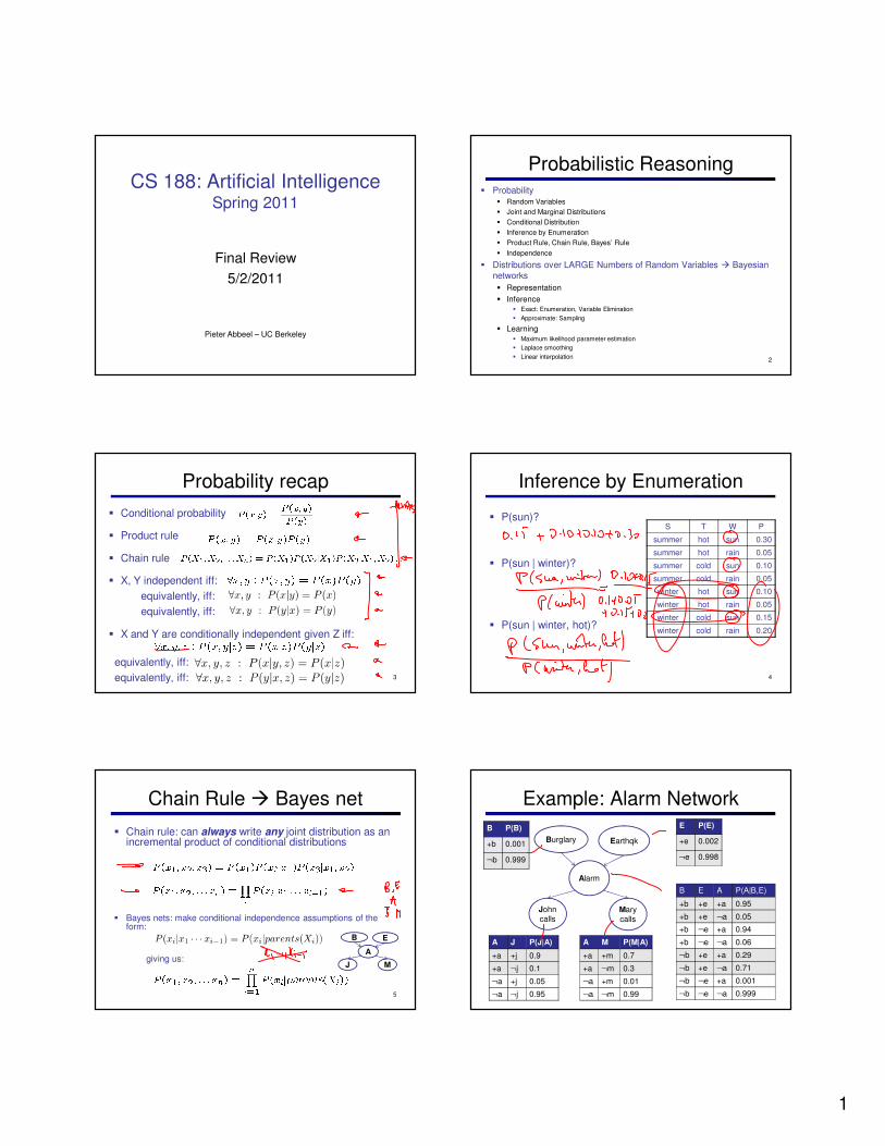
Probability recap

� Conditional probability

� Product rule

� Chain rule

� X, Y independent iff:

equivalently, iff:

equivalently, iff:

� X and Y are conditionally independent given Z iff:

equivalently, iff:

equivalently, iff: 3

Inference by Enumeration

� P(sun)?

� P(sun | winter)?

� P(sun | winter, hot)?

S T W P

summer hot sun 0.30

summer hot rain 0.05

summer cold sun 0.10

summer cold rain 0.05

winter hot sun 0.10

winter hot rain 0.05

winter cold sun 0.15

winter cold rain 0.20

4

Chain Rule � Bayes net

� Chain rule: can always write any joint distribution as an incremental product of conditional distributions

� Bayes nets: make conditional independence assumptions of the form:

giving us:

5

B E

A

J M

Example: Alarm Network

Burglary Earthqk

Alarm

John calls

Mary calls

B P(B)

+b 0.001

¬b 0.999

E P(E)

+e 0.002

¬e 0.998

B E A P(A|B,E)

+b +e +a 0.95

+b +e ¬a 0.05

+b ¬e +a 0.94

+b ¬e ¬a 0.06

¬b +e +a 0.29

¬b +e ¬a 0.71

¬b ¬e +a 0.001

¬b ¬e ¬a 0.999

A J P(J|A)

+a +j 0.9

+a ¬j 0.1

¬a +j 0.05

¬a ¬j 0.95

A M P(M|A)

+a +m 0.7

+a ¬m 0.3

¬a +m 0.01

¬a ¬m 0.99

2

Size of a Bayes’ Net for

� How big is a joint distribution over N Boolean variables?

2N

� Size of representation if we use the chain rule

2N

� How big is an N-node net if nodes have up to k parents?

O(N * 2k+1)

� Both give you the power to calculate

� BNs: � Huge space savings!

� Easier to elicit local CPTs

� Faster to answer queries 7

Bayes Nets: Assumptions

� Assumptions we are required to make to define the Bayes net when given the graph:

� Given a Bayes net graph additional conditional independences can be read off directly from the graph

� Question: Are two nodes necessarily independent given certain evidence?

� If no, can prove with a counter example

� I.e., pick a set of CPT’s, and show that the independence assumption is violated by the resulting distribution

� If yes, can prove with� Algebra (tedious)

� D-separation (analyzes graph) 8

D-Separation

� Question: Are X and Y conditionally independent given evidence vars {Z}?� Yes, if X and Y “separated” by Z� Consider all (undirected) paths

from X to Y

� No active paths = independence!

� A path is active if each triple is active:� Causal chain A → B → C where B

is unobserved (either direction)

� Common cause A ← B → C where B is unobserved

� Common effect (aka v-structure)A → B ← C where B or one of its descendents is observed

� All it takes to block a path is a single inactive segment

Active Triples Inactive Triples

D-Separation

� Given query

� Shade all evidence nodes

� For all (undirected!) paths between and

� Check whether path is active

� If active return

� (If reaching this point all paths have been checked and shown inactive)

� Return 10

?

Example

R

T

B

D

L

T’

Yes

Yes

Yes

11

All Conditional Independences

� Given a Bayes net structure, can run d-

separation to build a complete list of conditional independences that are

necessarily true of the form

� This list determines the set of probability

distributions that can be represented by Bayes’ nets with this graph structure

12

3

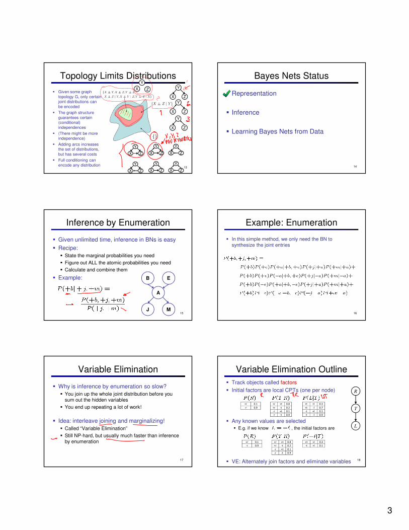
Topology Limits Distributions

� Given some graph

topology G, only certain joint distributions can

be encoded

� The graph structure

guarantees certain (conditional)

independences

� (There might be more

independence)

� Adding arcs increases the set of distributions,

but has several costs

� Full conditioning can

encode any distribution

X

Y

Z

X

Y

Z

X

Y

Z

13

X

Y

Z X

Y

Z

X

Y

Z X

Y

Z X

Y

Z

X

Y

Z

X

Y

Z

Bayes Nets Status

� Representation

� Inference

� Learning Bayes Nets from Data

14

Inference by Enumeration

� Given unlimited time, inference in BNs is easy

� Recipe:

� State the marginal probabilities you need

� Figure out ALL the atomic probabilities you need

� Calculate and combine them

� Example:

15

B E

A

J M

Example: Enumeration

� In this simple method, we only need the BN to synthesize the joint entries

16

Variable Elimination

� Why is inference by enumeration so slow?

� You join up the whole joint distribution before you sum out the hidden variables

� You end up repeating a lot of work!

� Idea: interleave joining and marginalizing!

� Called “Variable Elimination”

� Still NP-hard, but usually much faster than inference by enumeration

17

� Track objects called factors

� Initial factors are local CPTs (one per node)

� Any known values are selected

� E.g. if we know , the initial factors are

� VE: Alternately join factors and eliminate variables 18

Variable Elimination Outline

+r 0.1

-r 0.9

+r +t 0.8

+r -t 0.2

-r +t 0.1

-r -t 0.9

+t +l 0.3

+t -l 0.7

-t +l 0.1

-t -l 0.9

+t +l 0.3

-t +l 0.1

+r 0.1

-r 0.9

+r +t 0.8

+r -t 0.2

-r +t 0.1

-r -t 0.9

T

R

L

4

Variable Elimination Example

19

Sum out R

T

L

+r +t 0.08

+r -t 0.02

-r +t 0.09

-r -t 0.81

+t +l 0.3

+t -l 0.7

-t +l 0.1

-t -l 0.9

+t 0.17

-t 0.83

+t +l 0.3

+t -l 0.7

-t +l 0.1

-t -l 0.9

T

R

L

+r 0.1

-r 0.9

+r +t 0.8

+r -t 0.2

-r +t 0.1

-r -t 0.9

+t +l 0.3

+t -l 0.7

-t +l 0.1

-t -l 0.9

Join R

R, T

L

Variable Elimination Example

Join T Sum out TT, L L

* VE is variable elimination

T

L

+t 0.17

-t 0.83

+t +l 0.3

+t -l 0.7

-t +l 0.1

-t -l 0.9

+t +l 0.051

+t -l 0.119

-t +l 0.083

-t -l 0.747

+l 0.134

-l 0.886

Example

Choose A

21

Example

Choose E

Finish with B

Normalize

22

General Variable Elimination

� Query:

� Start with initial factors:� Local CPTs (but instantiated by evidence)

� While there are still hidden variables (not Q or evidence):� Pick a hidden variable H

� Join all factors mentioning H

� Eliminate (sum out) H

� Join all remaining factors and normalize

23

Approximate Inference: Sampling� Basic idea:

� Draw N samples from a sampling distribution S

� Compute an approximate posterior probability

� Show this converges to the true probability P

� Why? Faster than computing the exact answer

� Prior sampling:

� Sample ALL variables in topological order as this can be done quickly

� Rejection sampling for query

� = like prior sampling, but reject when a variable is sampled inconsistent with the query, in this case when a variable Ei is sampled differently from ei

� Likelihood weighting for query

� = like prior sampling but variables Ei are not sampled, when it’s their turn, they get set to ei, and the sample gets weighted by

P(ei | value of parents(ei) in current sample)

� Gibbs sampling: repeatedly samples each non-evidence variable conditioned on all other variables � can incorporate downstream evidence

24

5

Prior Sampling

Cloudy

Sprinkler Rain

WetGrass

Cloudy

Sprinkler Rain

WetGrass

25

+c 0.5

-c 0.5

+c +s 0.1

-s 0.9

-c +s 0.5

-s 0.5

+c +r 0.8

-r 0.2

-c +r 0.2

-r 0.8

+s +r +w 0.99

-w 0.01

-r +w 0.90

-w 0.10

-s +r +w 0.90

-w 0.10

-r +w 0.01

-w 0.99

Samples:

+c, -s, +r, +w

-c, +s, -r, +w

…

Example

� We’ll get a bunch of samples from the BN:

+c, -s, +r, +w

+c, +s, +r, +w

-c, +s, +r, -w

+c, -s, +r, +w

-c, -s, -r, +w

� If we want to know P(W)

� We have counts <+w:4, -w:1>

� Normalize to get P(W) = <+w:0.8, -w:0.2>

� This will get closer to the true distribution with more samples

� Can estimate anything else, too

� What about P(C| +w)? P(C| +r, +w)? P(C| -r, -w)?

� Fast: can use fewer samples if less time

Cloudy

Sprinkler Rain

WetGrass

C

S R

W

26

Likelihood Weighting

27

+c 0.5

-c 0.5

+c +s 0.1

-s 0.9

-c +s 0.5

-s 0.5

+c +r 0.8

-r 0.2

-c +r 0.2

-r 0.8

+s +r +w 0.99

-w 0.01

-r +w 0.90

-w 0.10

-s +r +w 0.90

-w 0.10

-r +w 0.01

-w 0.99

Samples:

+c, +s, +r, +w

…

Cloudy

Sprinkler Rain

WetGrass

Cloudy

Sprinkler Rain

WetGrass

Likelihood Weighting

� Sampling distribution if z sampled and e fixed evidence

� Now, samples have weights

� Together, weighted sampling distribution is consistent

Cloudy

R

C

S

W

28

Gibbs Sampling

� Idea: instead of sampling from scratch, create samples that are each like the last one.

� Procedure: resample one variable at a time, conditioned on all the rest, but keep evidence fixed.

� Properties: Now samples are not independent (in fact they’re nearly identical), but sample averages are still consistent estimators!

� What’s the point: both upstream and downstream variables condition on evidence.

29

Markov Models� A Markov model is a chain-structured BN

� Each node is identically distributed (stationarity)

� Value of X at a given time is called the state

� As a BN:

� The chain is just a (growing) BN� We can always use generic BN reasoning on it if we truncate the chain at a

fixed length

� Stationary distributions

� For most chains, the distribution we end up in is independent of the initial distribution

� Called the stationary distribution of the chain

� Example applications: Web link analysis (Page Rank) and Gibbs Sampling

X2X1 X3 X4

6

Hidden Markov Models

� Underlying Markov chain over states S

� You observe outputs (effects) at each time step

� Speech recognition HMMs:� Xi: specific positions in specific words; Ei: acoustic signals

� Machine translation HMMs:� Xi: translation options; Ei: Observations are words

� Robot tracking:� Xi: positions on a map; Ei: range readings

X5X2

E1

X1 X3 X4

E2 E3 E4 E5

Online Belief Updates

� Every time step, we start with current P(X | evidence)

� We update for time:

� We update for evidence:

� The forward algorithm does both at once (and doesn’t normalize)

X2X1

X2

E2

Particle Filtering

0.0 0.1

0.0 0.0

0.0

0.2

0.0 0.2 0.5

� = likelihood weighting + resampling at each time slice

� Why: sometimes |X| is too big to use exact inference

� Particle is just new name for sample

Particle Filtering

� Elapse time:� Each particle is moved by sampling its

next position from the transition model

� Observe:� We don’t sample the observation, we fix it

and downweight our samples based on the evidence

� This is like likelihood weighting, so we

� Resample:� Rather than tracking weighted samples,

we resample

� N times, we choose from our weighted sample distribution

Dynamic Bayes Nets (DBNs)

� We want to track multiple variables over time, using multiple sources of evidence

� Idea: Repeat a fixed Bayes net structure at each time

� Variables from time t can condition on those from t-1

� Discrete valued dynamic Bayes nets are also HMMs

G1a

E1a E1

b

G1b

G2a

E2a E2

b

G2b

t =1 t =2

G3a

E3a E3

b

G3b

t =3

Bayes Nets Status

� Representation

� Inference

� Learning Bayes Nets from Data

36

7

Parameter Estimation

� Estimating distribution of random variables like X or X | Y

� Empirically: use training data� For each outcome x, look at the empirical rate of that value:

� This is the estimate that maximizes the likelihood of the data

� Laplace smoothing� Pretend saw every outcome k extra times

� Smooth each condition independently:

r g g

Bayes Nets Status

� Representation

� Inference

� Learning Bayes Nets from Data

38

Classification: Feature Vectors

Hello,

Do you want free printr

cartriges? Why pay more

when you can get them

ABSOLUTELY FREE! Just

# free : 2

YOUR_NAME : 0

MISSPELLED : 2

FROM_FRIEND : 0

...

SPAMor+

PIXEL-7,12 : 1

PIXEL-7,13 : 0

...

NUM_LOOPS : 1

...

“2”

Classification overview

� Naïve Bayes:� Builds a model training data

� Gives prediction probabilities

� Strong assumptions about feature independence

� One pass through data (counting)

� Perceptron:� Makes less assumptions about data

� Mistake-driven learning

� Multiple passes through data (prediction)

� Often more accurate

� MIRA:� Like perceptron, but adaptive scaling of size of update

� SVM:� Properties similar to perceptron

� Convex optimization formulation

� Nearest-Neighbor:� Non-parametric: more expressive with more training data

� Kernels� Efficient way to make linear learning architectures into nonlinear ones

Bayes Nets for Classification

� One method of classification:

� Use a probabilistic model!

� Features are observed random variables Fi

� Y is the query variable

� Use probabilistic inference to compute most likely Y

� You already know how to do this inference

General Naïve Bayes

� A general naive Bayes model:

� We only specify how each feature depends on the class� Total number of parameters is linear in n� Our running example: digits

Y

F1 FnF2

|Y| parameters n x |F| x |Y| parameters

|Y| x |F|n

parameters

8

Bag-of-Words Naïve Bayes

� Generative model

� Bag-of-words� Each position is identically distributed

� All positions share the same conditional probs P(W|C)

� � When learning the parameters, data is shared over all positions in the document (rather than separately learning a distribution for each position in the document)

� Our running example: spam vs. ham

Word at position

i, not ith word in

the dictionary!

Linear Classifier

� Binary linear classifier:

� Multiclass linear classifier:

� A weight vector for each class:

� Score (activation) of a class y:

� Prediction highest score wins

Binary = multiclass where the

negative class has weight zero

Perceptron = algorithm to learn weights w

� Start with zero weights

� Pick up training instances one by one

� Classify with current weights

� If correct, no change!

� If wrong: lower score of wrong answer, raise score of right answer

45

Problems with the Perceptron

� Noise: if the data isn’t separable, weights might thrash� Averaging weight vectors over time

can help (averaged perceptron)

� Mediocre generalization: finds a “barely” separating solution

� Overtraining: test / held-out accuracy usually rises, then falls� Overtraining is a kind of overfitting

Fixing the Perceptron: MIRA

� Update size that fixes the current mistake and also minimizes the

change to w

� Update w by solving:

τ ≤ C

, τSVM

Support Vector Machines

� Maximizing the margin: good according to intuition, theory, practice

� Support vector machines (SVMs) find the separator with max margin

� Basically, SVMs are MIRA where you optimize over all examples at

once

SVM

9

Non-Linear Separators

� Data that is linearly separable (with some noise) works out great:

� But what are we going to do if the dataset is just too hard?

� How about… mapping data to a higher-dimensional space:

0

0

0

x2

x

x

x

This and next few slides adapted from Ray Mooney, UT

49

Non-Linear Separators

� General idea: the original feature space can always be mapped to some higher-dimensional feature space where the training set is separable:

Φ: x→ φ(x)

50

Some Kernels

� Kernels implicitly map original vectors to higher dimensional spaces, take the dot product there, and hand the result back

� Linear kernel:

� Quadratic kernel:

51

φ(x) = x

Some Kernels (2)

� Polynomial kernel:

Why and When Kernels?

� Can’t you just add these features on your own (e.g. add all pairs of features instead of using the quadratic kernel)?� Yes, in principle, just compute them

� No need to modify any algorithms

� But, number of features can get large (or infinite)

� Kernels let us compute with these features implicitly� Example: implicit dot product in polynomial, Gaussian and string

kernel takes much less space and time per dot product

� When can we use kernels?� When our learning algorithm can be reformulated in terms of

only inner products between feature vectors� Examples: perceptron, support vector machine

K-nearest neighbors

� 1-NN: copy the label of the most similar data point

� K-NN: let the k nearest neighbors vote (have to devise a weighting scheme)

� Parametric models:

� Fixed set of parameters

� More data means better settings

� Non-parametric models:

� Complexity of the classifier increases with data

� Better in the limit, often worse in the non-limit

� (K)NN is non-parametric

Truth

2 Examples 10 Examples 100 Examples 10000 Examples

54

10

Basic Similarity

� Many similarities based on feature dot products:

� If features are just the pixels:

� Note: not all similarities are of this form55

Important Concepts

� Data: labeled instances, e.g. emails marked spam/ham� Training set

� Held out set� Test set

� Features: attribute-value pairs which characterize each x

� Experimentation cycle� Learn parameters (e.g. model probabilities) on training set� (Tune hyperparameters on held-out set)� Compute accuracy of test set

� Very important: never “peek” at the test set!

� Evaluation� Accuracy: fraction of instances predicted correctly

� Overfitting and generalization� Want a classifier which does well on test data� Overfitting: fitting the training data very closely, but not

generalizing well� We’ll investigate overfitting and generalization formally in a

few lectures

TrainingData

Held-OutData

TestData

Tuning on Held-Out Data

� Now we’ve got two kinds of unknowns

� Parameters: the probabilities P(Y|X), P(Y)

� Hyperparameters:

� Amount of smoothing to do: k, α (naïve Bayes)

� Number of passes over training data (perceptron)

� Where to learn?

� Learn parameters from training data

� Must tune hyperparameters on different data

� For each value of the hyperparameters, train and test on the held-out data

� Choose the best value and do a final test on the test data

Extension: Web Search

� Information retrieval:

� Given information needs, produce information

� Includes, e.g. web search, question answering, and classic IR

� Web search: not exactly classification, but rather ranking

x = “Apple Computers”

Feature-Based Ranking

x = “Apple Computers”

x,

x,

Perceptron for Ranking

� Inputs

� Candidates

� Many feature vectors:

� One weight vector:

� Prediction:

� Update (if wrong):