Embed Size (px)
Citation preview

SDR Implementation of a OFDM-MIMO Receiver
MASTER THESIS
10TH
SEMESTER 2008 PROJECT, AAU
APPLIED SIGNAL PROCESSING
AND IMPLEMENTATION (ASPI)
Group 1046
Morris Filippi

2

3
Abstract:
The word diversity, in telecommunication,
means MIMO systems, that is transmitting
the signals through multiple antennas
(Multiple Input Multiple Output), and it
can be performed in various domains, such
as space and time. Thanks to MIMOs (i.e.
Spatial Multiplexing, Space-Time Coding)
is possible to increase the bit-rate
maintaining the same implementation
constraints, as transitting power and
bandwidth availability. These diversity
techniques exploit the redundant
transmission of data on the various
antennas, allowing the decoding at the
receiption by precise algorithms.
The purpose of this project was to identify
which type of algorithmic improvements
can be used to increase the spectral
efficiency of an OFDM/MIMO receiver,
while maintaining its HW feasibility.
In this report, the designer propose a
possible solution to the problem statement.
This is the identification of two new
techniques, which are conceived to solve
the central problem of the MIMO with
more than two transmitting antennas: the
quasi-orthogonality of product between
channel matrix and its Hermitian. This
report contains the implementation steps in
order to converge to a feasible hardware
solution, starting from the initial problem
to the final simulations and SW/HW co-
simulation.
Title:
SDR Implementation of a
OFDM-MIMO Receiver
Theme:
OFDM - MIMO Algorithms and
Architectures, Optimal VLSI Signal
Processing
Project period:
P10, spring semester 2009
01/02/09 - 30/06/09
Project group:
ASPI 09gr1046
Group member:
Morris Filippi
Supervisors:
Yannick Le Moullec (AAU)
Andrea Fabio Cattoni (AAU, Nokia-Siemens)
Copies: 4 + 4 CD-ROM
Number of pages in Report:
Number of words:
Finished: 03/06/09

4

5
Preface
This report serves as documentation for the 10th semester project in “Applied Signal
Processing and Implementation” (ASPI) at the Institute of Electronic Systems of Aalborg
University (AAU). The project is a “Software Defined Radio Implementation of a MIMO
Receiver with two switchable modes”, made by the group 1046. The work is co-supervised
by the Software Defined Radio Center (CSDR) division of Aalborg University.
The report consists in three main parts:
Analysis, that treats the methodology Rugby Meta-Model, the OFDM, MIMO and SDR
theory;
Design, which contains the development steps of the receiver’s implementation;
Evaluations, which explains the results obtained, the possible future implementations
and the conclusions.
The software used are: MatLab, Simulink, System Generator.
................................ (signature)
Morris Filippi

6
7
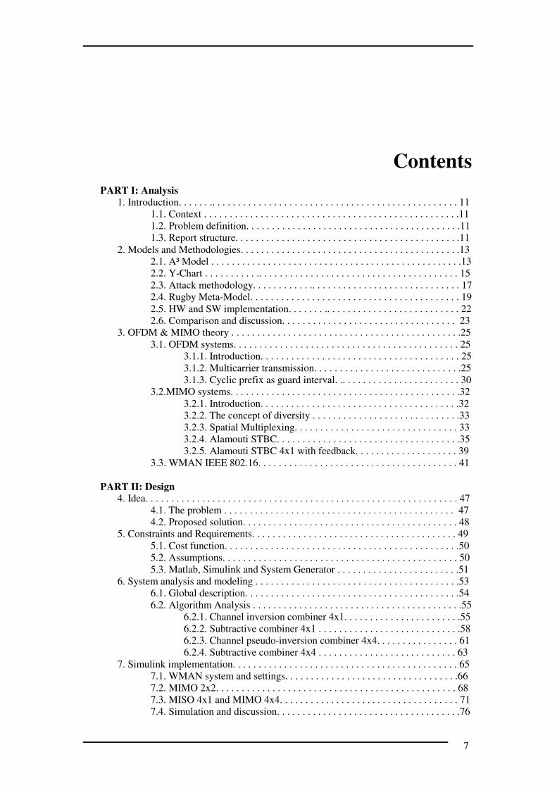
Contents
PART I: Analysis
1. Introduction. . . . . . .. . . . . . . . . . . . . . . . . . . . . . . . . . . . . . . . . . . . . . . . . . . . . . . . 11
1.1. Context . . . . . . . . . . . . . . . . . . . . . . . . . . . . . . . . . . . . . . . . . . . . . . . . . .11
1.2. Problem definition. . . . . . . . . . . . . . . . . . . . . . . . . . . . . . . . . . . . . . . . . .11
1.3. Report structure. . . . . . . . . . . . . . . . . . . . . . . . . . . . . . . . . . . . . . . . . . . .11
2. Models and Methodologies. . . . . . . . . . . . . . . . . . . . . . . . . . . . . . . . . . . . . . . . . . .13
2.1. A³ Model . . . . . . . . . . . . . . . . . . . . . . . . . . . . . . . . . . . . . . . . . . . . . . . . .13
2.2. Y-Chart . . . . . . . . . . .. . . . . . . . . . . . . . . . . . . . . . . . . . . . . . . . . . . . . . . 15
2.3. Attack methodology. . . . . . . . . . . .. . . . . . . . . . . . . . . . . . . . . . . . . . . . . 17
2.4. Rugby Meta-Model. . . . . . . . . . . . . . . . . . . . . . . . . . . . . . . . . . . . . . . . . 19
2.5. HW and SW implementation. . . . . . . .. . . . . . . . . . . . . . . . . . . . . . . . . . 22
2.6. Comparison and discussion. . . . . . . . . . . . . . . . . . . . . . . . . . . . . . . . . . 23
3. OFDM & MIMO theory . . . . . . . . . . . . . . . . . . . . . . . . . . . . . . . . . . . . . . . . . . . . .25
3.1. OFDM systems. . . . . . . . . . . . . . . . . . . . . . . . . . . . . . . . . . . . . . . . . . . . 25
3.1.1. Introduction. . . . . . . . . . . . . . . . . . . . . . . . . . . . . . . . . . . . . . . 25
3.1.2. Multicarrier transmission. . . . . . . . . . . . . . . . . . . . . . . . . . . . .25
3.1.3. Cyclic prefix as guard interval. .. . . . . . . . . . . . . . . . . . . . . . . 30
3.2.MIMO systems. . . . . . . . . . . . . . . . . . . . . . . . . . . . . . . . . . . . . . . . . . . . .32
3.2.1. Introduction. . . . . . . . . . . . . . . . . . . . . . . . . . . . . . . . . . . . . . .32
3.2.2. The concept of diversity . . . . . . . . . . . . . . . . . . . . . . . . . . . . .33
3.2.3. Spatial Multiplexing. . . . . . . . . . . . . . . . . . . . . . . . . . . . . . . . 33
3.2.4. Alamouti STBC. . . . . . . . . . . . . . . . . . . . . . . . . . . . . . . . . . . .35
3.2.5. Alamouti STBC 4x1 with feedback. . . . . . . . . . . . . . . . . . . . 39
3.3. WMAN IEEE 802.16. . . . . . . . . . . . . . . . . . . . . . . . . . . . . . . . . . . . . . . 41
PART II: Design 4. Idea. . . . . . . . . . . . . . . . . . . . . . . . . . . . . . . . . . . . . . . . . . . . . . . . . . . . . . . . . . . . . 47
4.1. The problem . . . . . . . . . . . . . . . . . . . . . . . . . . . . . . . . . . . . . . . . . . . . . 47
4.2. Proposed solution. . . . . . . . . . . . . . . . . . . . . . . . . . . . . . . . . . . . . . . . . . 48
5. Constraints and Requirements. . . . . . . . . . . . . . . . . . . . . . . . . . . . . . . . . . . . . . . . 49
5.1. Cost function. . . . . . . . . . . . . . . . . . . . . . . . . . . . . . . . . . . . . . . . . . . . . .50
5.2. Assumptions. . . . . . . . . . . . . . . . . . . . . . . . . . . . . . . . . . . . . . . . . . . . . . 50
5.3. Matlab, Simulink and System Generator . . . . . . . . . . . . . . . . . . . . . . . .51
6. System analysis and modeling . . . . . . . . . . . . . . . . . . . . . . . . . . . . . . . . . . . . . . . .53
6.1. Global description. . . . . . . . . . . . . . . . . . . . . . . . . . . . . . . . . . . . . . . . . .54
6.2. Algorithm Analysis . . . . . . . . . . . . . . . . . . . . . . . . . . . . . . . . . . . . . . . . .55
6.2.1. Channel inversion combiner 4x1. . . . . . . . . . . . . . . . . . . . . . .55
6.2.2. Subtractive combiner 4x1 . . . . . . . . . . . . . . . . . . . . . . . . . . . .58
6.2.3. Channel pseudo-inversion combiner 4x4. . . . . . . . . . . . . . . . 61
6.2.4. Subtractive combiner 4x4 . . . . . . . . . . . . . . . . . . . . . . . . . . . 63
7. Simulink implementation. . . . . . . . . . . . . . . . . . . . . . . . . . . . . . . . . . . . . . . . . . . . 65
7.1. WMAN system and settings. . . . . . . . . . . . . . . . . . . . . . . . . . . . . . . . . .66
7.2. MIMO 2x2. . . . . . . . . . . . . . . . . . . . . . . . . . . . . . . . . . . . . . . . . . . . . . . 68
7.3. MISO 4x1 and MIMO 4x4. . . . . . . . . . . . . . . . . . . . . . . . . . . . . . . . . . . 71
7.4. Simulation and discussion. . . . . . . . . . . . . . . . . . . . . . . . . . . . . . . . . . . .76

8
8. System Generator implementation . . . . . . . . . . . . . . . . . . . . . . . . . . . . . .. . . . . . .77
8.1. Motivations. . . . . . . . . . . . . . . . . . . . . . . . . . . . . . . . . . . . . . . . .. . . . . . .78
8.2. SysGen blocks and sub-system used. . . . . . . . . . . . . . . . . . . . . . . . . . . .79
8.3. SysGen STBC 4x4 subtractive combiner. . . . . . . . . . . . . . . . . . . . . . . . 81
8.4. SysGen Resource Estimator. . . . . . . . . . . . . . . . . . . . . . . . . . . . . . . . . . 85
9. Hardware Implementation. . . . . . . . . . . . . . . . . . . . . . . . . . . . . . . . . . . . . . . . . .. . . . . .87
9.1. ML506 board. . . . . . . . . . . . . . . . . . . . . . . . . . . . . . .. . . . . . . . . . . . . . . 88
9.2. SW/HW co-simulation. . . . . . . . . . . . . . . . . . . . . . . . . . . . . . . . . . . . . . 88
PART III: Evaluations 10. Tests & Validations. . . . . . . . . . . . . . . . . . . . . . . . . . . . . . . . . . . . . . . . . . . . . . . .95
10.1. Simulink simulations. . . . . . . . . . . . . . . . . . . . . . . . . . . . . . . . . . . . . . .95
10.2. SysGen simulations. . . . . . . . . . . . . . . . . . . . . . . . . . . . . . . . . . . . . . . .97
10.3. SW/HW co-simulation. . . . . . . . . . . . . . . . . . . . . . . . . . . . . .. . . . . . . .99
11. Conclusion. . . . . . . . . . . . . . . . . . . . . . . . . . . . . . . . . . . . . . . . . . . . . . . . . . . . . .103
11.1. Future work . . . . . . . . . . . . . . . . . . . . . . . . . . . . . . . . . . . . . . . . . . . . .104
Bibliography. . . . . . . . . . . . . . . . . . . . . . . . . . . . . . . . . . . . . . . . . . . . . . . . . . . . . . . . . . .105
Appendix A. . . . . . . . . . . . . . . . . . . . . . . . . . . . . . . . . . . . . . . . . . . . . . . . . . . . . . . . . . . 107
Appendix B. . . . . . . . . . . . . . . . . . . . . . . . . . . . . . . . . . . . . . . . . . . . . . . . . . . . . . . . . . . 109
Appendix C. . . . . . . . . . . . . . . . . . . . . . . . . . . . . . . . . . . . . . . . . . . . . . . . . . . . . . . . . . . 115
Appendix D. . . . . . . . . . . . . . . . . . . . . . . . . . . . . . . . . . . . . . . . . . . . . . . . . . . . . . . . . . . 116

9
Part I
Analysis

10

11
1. Introduction
1.1. Context
In the last twenty years the concept of distance has changed in many fields, talking about
depth perception and not in the physical sense, of course. That can mean how far the people
feel in term of humanistic relationship and in this field the communication is one of the main
factors. The technology provided the media to realize this improvement, through new
structures which allowed to communicate almost anywhere, at everytime and with anyone [1].
More precisely these technical supports can be classified as wireless communication.
Today, the wireless communications support many applications, such as satellites, inter-
continental, middle-frequency and local connections. Focusing on the last, the local
communication, it is well note that the wireless is applied capillarly, at the end of the network.
This because the wireless channel is more restrictive respect to the cable connection [13], so
shorter the distance between antennas, higher the data-rate allowed. In this direction have
been developed local and metropolitan wireless systems, WLAN and WMAN respectively.
These networks provide high bit-rate in order to satisfy the functionalities of the last-
generation devices, where the key word is convergence of services: cellular phone, GPS, TV
and computer.
A technique largely used in the wireless communication is the OFDM (Orthogonal
Frequency Division Multiplexing), which supports the WLAN IEEE 802.11a, g, n,
HIPERLAN, DVB-T, DVB-H, UMTS generation, WiMAX IEEE 802.16 and many others.
These examples show that the OFDM is employed in most of the last telecommunication
systems, explored and improved in all its parts. That is the why the actual research tries to
mix other technique with the OFDM, to speed up the two main requirements of high bit-rate
and low probability of errors.
In this direction, applying the diversity principles to the OFDM digital multi-carrier
modulation is certanly one of the future perspective. The word diversity, in
telecommunication, means MIMO systems, that is transmitting the signals through multiple
antennas (Multiple Input Multiple Output), and it can be performed in various domains, such
as space and time. Thanks to MIMOs (i.e. Spatial Multiplexing, Space-Time Coding) is
possible to increase the bit-rate maintaining the same implementation constraints, as
transitting power and bandwidth availability. These diversity techniques exploit the redundant
transmission of data on the various antennas, allowing the decoding at the receiption by
precise algorithms.
1.2. Problem definition
Considering the already existing MIMO applications:
“what type of algorithmic improvements can be used to increase the spectral efficiency of an
OFDM/MIMO receiver, while maintaining its HW feasibility?”
1.3. Report structure
The report is organized in three main parts, identified by Analysis, Design and Evaluation.
The first part starts with the introduction chapter, that contains this project context, and it

12
focuses on the problem statement. It follows the chapter concerning the methodologies and
methods. In this, a comparison between various methodologies is reported, with the final
choise for Rugby Meta-Model [4], [6]. The third chapter consists in the theoretical overview
related to this project, with sub-sections on OFDM and MIMOs.
The second part is the Design and is divided in steps following Rugby Meta-Model. The
initial idea presents the proposed solution for this project. Chapter 5 indicates the cost
function and the other constraints. The sixth chapter contains the system analysis and
proposes two new algorithms for QO-MIMO receivers. The following chapter illustrates the
Simulink implementation of the proposed techniques. Chapter 8 focuses on one of these
techniques reporting the development of the System Generation implementation. Finally,
Chapter 9 treats the hardware implementation by a co-simulation point of view.
The last part, Evaluation, starts with the Results chapter. It contains the presentation and
the discussion on the partial and final simulations. Moreover it treats the SW/HW co-
simulation using the target FPGA. Chapter 11 is the conclusion and the proposed future
implementation starting from the work done in this project.

13
2. Models and Methodologies
In this chapter a short description of some models and methodologies is done. This
because developing a project by following a certain structure is useful, when it is multi-
tasking and complex. Dividing the work in activities and sub-task allows a better organization
during the implementation and gives an indication on the eventual delays in the project.
Moreover, through various domains, it is possible to describe and classify the implementation
steps.
The first part of this chapter treats the A3 Model [2] and the fitting to this project. The
second part reports some methodologies with a final comparison and following choice for this
application.
2.1. A3 Model
The A3 Model is a paradigm conceived at Aalborg University [2], developed for
electronic system design. The main purpose of the A3 model is to give a first structure and a
trajectory to the project that is going to be implemented, by the classification in three
domains of the requirements and the developing environment. As shown in Figure 2.1 for a
generic diagram, these three domains are Applications, Algorithms and Architectures, which
give the name A3 to this paradigm.
Figure 2.1: A generic sheme of A3 paradigm, composed by the three domains: Applications,
Algorithms and Architectures. The relations between them converge to a Fit line, inspired by
the figure in slide 3 [2].
Starting from the application that has to be implemented, the model allows to connect it
to one or more algorithms by applying linear or non-linear signal processing [2]. The second
step is to modify the applications in relation to eventually troubles or unfeasibility, that could
Algorithms
Architectures
feedback
feedback
Fit line
Constraints & Requirements
Implementation
Numbers & Results
Applications

14
mean adding some constraints. After that, the model shows possible architectural solutions
for the algorithms, which can be more than one as for the first case, so finally it can lead to a
large design space [2]. This phase is processed by HW-SW codesign and architecture
exploration [2]. Analyzing the various point in the Architectures domain, there is a feedback
to the previous Algorithms for the validation.
After the implementation, verifying the results is necessary, so as seen in Figure 2.1, the
A3 Model inspects if the final tests respect the initial constraints and satisfy the requirements.
This take place on the Fit line.
Note that the various A3 domains can be subdivided in sets which are defined by the target
constraints, such as hardware platforms, in case of Architectures, or recursive functions for
Algorithms (this concept is better shown in Figure 2.2).
Applying the A3 Model to this project, the scheme in Figure 2.2 is obtained. The initial
idea is to implement a wireless system based on the IEEE 802.16 standard, a Wireless
Metropolitan Area Network (WMAN), the Worldwide Interoperability for Microwave Access
(WiMAX). In particular the project focuses on the physical link, by the insertion of a MIMO
system in the original OFDM scheme in order to speed up the bit-rate and to reduce the
probability of errors.
Figure 2.2: A3 Paradigm applied to this project. The scheme shows the relations between the
three domains and the high level possible solutions.
feedback
feedback
Fit line
Constraints & Requirements
Implementation
Numbers & Results
Applications
Modulation
WMAN
OFDM-
MIMO
Algorithms
Architectures
[BPSK,QPSK,{16,64}-QAM]
[Alamouti {2x2, 4x1, 4x4}]
FPGA
Target: Xilinx
FPGA
Virtex 5 cx5vsx50t
DSP
GPP
Computer

15
The second domain, Algorithms, shows the different modulations that the physical link
must support and on the other hand the types of MIMO that should be implemented. Note that
the transmitting Alamouti mode is an initial constraint. The algorithms MISO 2x1 (with two
transmitting and one receiving antennas) is provided as basis by [24] and [26], and the
purpose of the project is to implement other, more advanced, MIMO modes such as the 2x2
and the so-called extended-MIMOs 4x1 and 4x4.
The Architectures domain points out the possible hardware solutions, with the constraint
target Xilinx Virtex 5 FPGA cx5vsx50t, but note that the scheme indicates other possible HW
devices. This because doing a high level estimation on the computational complexity, results
impossible to implement all the WiMAX and MIMO physical layer on the FPGA indicated,
which features are well-known. At this initial phase of the project, the purpose is to start by
implementing just the MIMO algorithm on FPGA and study the feasibility to add other parts.
Eventually replace the target FPGA with a DSP more powerful.
2.2. Y-Chart Methodology
The Y-Chart Methodology [3] and [4] has been developed in the 80’s, when the numbers
of transistors in electronic design, began to be too large to be managed enterly by humans. It
gives a top-down guidelines for the VLSI design by a Y-shaped structure, as shown in Figure
2.3. The Y-Chart is divided in three domains which are represented by three respective axes,
functional, structural and geometrical. Each one is divided in sub-levels.
� Functional, is at the highest abstraction level and defines the mathematical
expressions in boolean format. This domain does not specify any physical aspect
such as computational devices or connections. Note that the Functional
representation is also called Behavioural. This second definition is chosen.
� Structural, is the middle domain which consists in a graphic representation of the
expressions defined on the Behavioural axis. By mapping this functions, a group of
connected components is obtained. The synthesis is done by considering a cost
function, that can contain area, execution time, energy consumption, etc.
� Geometrical, is the lowest level of the methodology, which specifies the physical
design considering various constraints as dimension of the electronic components
and the wires between them.
Figure 2.3: Y-Chart Methodology, generic representation of the three domains and the
respective possible levels. Inspired by Figure 2 [3].
STUCTURAL BEHAVIOURAL Synthesis
Processor
Memory Technology Logic Systems
Switch Check Verification
Register Algorithmic
Transfer
Boolean
Circuit Expressions
Physical-to-logical Check
Place & Routing
Mask Geometries
Cells
Topology Check
Layout
Planning
GEOMETRICAL

16
The activity starts from the extreme of the Behavioural axis, the designer translates the
expressions by using hand or automatic synthesis, obtaining the first step of the Structural
domain. These actions by connecting archs is represented, creating a circular trend around the
Y-Chart. Note that at the end of every synthesis, a verification is done, as shown in Figure 2.3.
The Y-Chart can be fitted to this project identifying the possible steps on the three
domains. The result is the scheme in Figure 2.4, where the various synthesis archs have been
omitted for graphical reasons.
Figure 2.4: Y-Chart Methodology adapted to this projec, with the various levels. Inspired by
Figure 2 [3] and Figure 1 [4] .
The adapted Y-Chart shown in Figure 2.4 has additional levels on its axes, necessary to
split in variouos implementation steps. The first level of the Behavioural domain indicates the
OFDM-MIMO functionalities, followed by the modulations and the multiple antennas
systems, the algorithms which describes the whole system and the lower boolean functions.
Finally the transistor physical equations.
The Structural domain reports the components at various abstraction levels with the
functional connections. Note that the number of unities considered increases towards the
center of the Y.
The Geometrical representation reports the physical connections at the respectives level
of components considered. From the highest level there are Layout Planning, Clusters, Floor
Plans, Mask Geometries and Physical Layout. But note that in this project the FPGA is
already manufactured and it is programmed through automatic mapping, place & route and
bit-stream generation.
STUCTURAL BEHAVIOURAL
Xilinx FPGA,
Memory OFDM
MIMO
Register 2x2, 4x1
HW modules 4x4, modulations
Operators Algorithms
ALUs, MUXs, Reg
Slices, LUT Boolean Function
Circuit Transistor Equations
Physical Layout
Mask Geometries
Floor Plans,
Connections
Clusters
The FPGA is already manufactured
programmed by atomatic compiler
Layout
Planning
GEOMETRICAL

17
2.3. ATtACk Methodology
Attack [5] is a methodology based on the Rugby Meta-Model [6], discussed in 2.4,
conceived to extend this model to dynamic partially reconfigurable systems on FPGA. The
name ATtACk derives from the four domains which compose the methodology: Algorithm,
Time, Architecture and Communication. A second flow specifies the four phases, common
for each domain: Specification and Requirements, System Model, Design and
Implementation. Figure 2.5 shows the methodology graph, with an overview of the domain
levels.
Figure 2.5: ATtACk Methodology, a generic case of implementation, with the four domains
and four phases. Inspired by Figure 2 [5].
The four domains which compose the Attack methodology are now described.
� Algorithm, specifies the various mathematical expressions and correlations. Note
that for the partial reconfiguration these algorithms must be two or more. The
first step is to analyze the documentations and background in order to identify the
subjects, second translate them to Control Data Flow Graphs (CDFGs) to list the
execution steps. By examining the CDFGs it is possible to identify the two
modules, static and dynamic, for the partial reconfiguration.
� Architecture, defines the hardware platform where the algorithms have to execute.
At first it is necessary to identify the possible device analyzing the various
features, as i.e. the FPGA chip, the In/Out ports, memory and interface devices
(i.e. ADC/DAC, audio ports, etc.). The second phase is to identify the parts of the
platform which compute the algorithms. Third, the FPGA can be divided in static
and dynamic areas to perform the eventual partial reconfiguration, so it is
necessary to use special tools provided by the FPGA producers, such as PR flow
from Xilinx [36].
� Communication, treats every signal that transfers data, address and control
information, considering the connections and the data format. This domain allows
TIME COMMUNICATION
Constraints Input & Output
Causality Entity Interface
Configuration Time Inter module comm.
Physical Clock Busses
Target
Programming Pin out config. IMPLEMENTATION
Modules PE partitioning DESIGN
Flow Chart Entities
SYSTEM MODEL
Functionality Platform
ALGORITHM ARCHITECTURE SPECIFICATION AND
REQUIREMENTS

18
to identify the links on the platform, inputs and outputs. Second step is to connect
the functional blocks having a look on the static and dynamic areas. Finally the
platform has to be linked to the testing environment, that could be a tool for co-
simulation running on a computer.
� Time, treats all the information regarding the execution time of the system at the
various abstraction levels. Initially there are generic constraints only, the next
level expresses causality between the steps of the CDFG. At the third level the
operators and the connections can introduce delays that have to be considered.
Finally the delays of the physical components and wires, but also the
reconfiguration time to change between dynamic blocks are expressed.
The Attack methodology has been conceived for dynamic partial reconfiguration, but can
be adapted to this project, considering that this FPGA’s functionality is not used. Figure 2.6
shows a possible fit for this project.
Figure 2.6: ATtACk Methodology applied to this project, with the four domains and an
additional phase (Xilinx design) in the design step. Inspired by Figure 2 [5].
Some part of the scheme shown in Figure 2.5, for this customized version are maintained.
As already reported, adapting the Attack methodology to this project requires a modification
of the design phase. Figure 2.6 shows that the third phase has been split in two phases, in
Figure 2.5, Matlab Simulink design and Xilinx System Generator (SysGen) oriented design.
In fact, even if the development environment is the same, Matlab Simulink, the libraries
changes, and that means the operators change. In the Simulink Design phase the operators are
standard blocks, S-functions and Matlab-functions, and for the following phase the
components are Xilinx blocks at lower abstraction level. So, some part of the project scheme
have to be translated manually using basic operators.
In Figure 2.6 for the two design phases, the same level on the four domains is shown, but
note that both of them can have different Operators, Inter module communications, and
Sample Times. On the other hands, the Operations must remain the same.
TIME COMMUNICATION
Constraints Input & Output
Causality Unit interfaces
Sample Time Inter module comm.
Physical Clock Links
Target
Programming Pin out config. IMPLEMENTATION
Operations XILINX SYSGEN DESIGN Operators
SIMULINK DESIGN
Flow Chart Performing units
SYSTEM MODEL
Modulations Target Platform
[2x2, 4x1,4x4] Xilinx Virtex 5
ALGORITHM SPECIFICATION AND ARCHITECTURE REQUIREMENTS

19
2.4. Rugby Meta-Model
The Rugby Meta-Model [4] and [6] is a methodology for electronic system design based
on the Y-Chart [3] and [4], but it extends the domains in order to manage more complex
systems, as those which present hardware and software implementation. Rugby is divided by
four domains, Computation, Communication, Data and Time, each split into phases. These
phases correspond to different levels of abstraction. The Rugby methodology can consider
split or mixed HW/SW implementation, in this report, only the mixed version is explained.
An important comparison between two similar concepts are treated:
� Hierarchy, which is the subdivision of the design models in steps. Each step
indicates the amount of information used to describe the system, while other
details are hidden.
� Abstraction, which specifies the models and the semantics used in a project at
various steps. These models represent the behaviour of the components used to
describe the system, and at each level information are respectively detailed.
While the abstraction levels are pre-defined for every HW/SW implementation, the
hierarchy is a designer choice, for instance each abstraction level and domain can represent a
hierarchical step. Because of this general concept, Hierarchy is not explicitly specified in the
Rugby Meta-Model.
Figure 2.7: The Rugby Meta-Model, a generic scheme that shows the starting point (initial
idea), the arrival point (physical system), four domains (computation, communication, data,
time), and the two trend lines (abstraction and time). Inspired by Figure 4 [4].
As already mentioned, Rugby is based on the Y-chart, but is extended in the domains. In
fact in this methodology the domains are four instead of three, and treat different fields:
� Computation, which indicates the mathematical expressions and relations
between data inputs and outputs. For each abstraction level, these computations
assume different descriptions, which are related to the considered component. For
instance at physical level, as the interactions between transistors, resistors,
capacities, the computations are differential equations that indicate the behaviour
of the electric current in relation to the voltage. Another example, at high
abstraction level, is the algorithm that a block can perform considering analog or
digital components, as amplifiers or modulators, etc.

20
� Communication, which specifies the links between the various components of the
design. These connections can be a functional link between main blocks or, for
instance, physical wires from a resistence to the gate of a silicon transistor,
considering a very low abstraction level. Moreover, these connections can
support various types of information, as controls, data, addresses.
� Data, which reports the types of data and the quantities that are computed. At an
intermediate abstraction level, the data can be real or imaginary numbers, defined
in time or frequency domain. Considering logical level, data are boolean values,
and at transistor level are real numbers which indicate the voltage or other
physical quantities.
� Time, which indicates the time-relation between components and, as in the others
domains, for the various abstraction levels is defined. In fact, every component
needs its computation time and every connection its delay, so these behaviours
have to be considered in the design. Note that at software level, the causality
relation only is treated.
The Rugby Meta-Model can be adapted to this project as for the previously considered
methodologies (Attack, Y-Chart). As already indicated, the Rugby mixed HW/SW only is
treated, because this project has not split implementation but a sequential software-hardware
flow.
Figure 2.8: Rugby Meta-Model, the scheme adapted for this application. The Abstraction line
has been divided in eight levels. Inspired by Figure 4 [4].
Figure 2.8 represents the scheme of Rugby fitted to this project. There is a sub-division of
the abstraction line in eight steps, starting from the initial idea to the physical implementation.
In Constraints & Requirements there is an indication about the main contents, the target
Xilinx FPGA and the various SIMO/MIMO schemes. The same goes for System Analysis &
Modeling, where the main parts of the system are shown. The fourth step consists in the
implementation of the system by using the development program Matlab and the grafic tool
Simulink, with the standard libraries provided by Mathworks. This step has been split from

21
the following abstraction level called System Generator, because even if the environment
used is Simulink, the libraries are provided by Xilinx. Moreover, this second software
implementation, has been separated because the components provided are hardware-
dedicated, meaning that they are operators at a lower abstraction level. By these Xilinx
System Generator’s blocks it is possible to translate directly the Simulink scheme in VHDL
code, so thanks to this powerful compiler, the intermediate steps to the FPGA implementation
are automated. Note that the Xilinx System Generator blocks are used just for some parts of
the system, in particular on the SIMO/MIMO receiver. Hardware implementation is the step
where the system is implemented on the target Xilinx Virtex 5 FPGA, with the simulation
environment building for the tests. Before the last On-chip receiver, there is Tests &
Validation, which consists in several simulations (or HW/SW co-simulations) to verify the
correct behaviour of the hardware system. Moreover, it is possible to compare the delays and
the approximation errors due to the difference between software and hardware. In fact very
often, a HW implementation requests the use of fixed point operations and bit-limited
solutions. Note that in Figure 2.8 the four typical domains of Rugby have been omitted for
graphic reasons, but they are actually considered in this project.
Analyzing in detail the Rugby scheme of this project, it is possible to define various steps
for the four domains, as done for the Y-Chart and the Attack methodologies. Figure 2.9
represents these intermediate levels on separated lines, in order to extend the Rugby shape,
applied to this project.
Figure 2.9: The Rugby Meta-Model’s domains fitted to this application. The various steps
indicate the details corresponding to the abstraction levels. Inspired by Figure 5 [4].
Xilinx Virtex5 OFDM transceiver Simulink Physical
FPGA, multiple antennas standard blocks, Sys Gen blocks, Slices, wires, Layout &
Matlab SW Rayleigh Channel interblocks links interblocks links HW operators connections
Communication
Modulations, Data packing, SysGen operations, Tests
SIMO/MIMO OFDM functions, IFFT/FFT, Matlab-Xilinx physical HW ops HW&SW
algorithms Alamouti, Rayleigh Matlab functions functions operations
Computation
Input/Output Data type Matlab accuracy SysGen accuracy
constraints, complex, floating point, fixed point, Logic values Analog
frame structure matrix complex bit-limited signals
Data
Sample time, SysGen Physical
Tx time Causality modulation delays, wire & slices Synchro.,
Speed up between blocks rates sample time dalays, clock clock, cycles
Time
Abstraction line High level Low level

22
The four domains defined by the lines in Figure 2.9, report the details considered for the
various abstraction levels. Note that the Communication and Data axes indicate main groups,
because the number of objects to consider are often very large. This kind of representation on
linear axes is simply adaptable in case of HW/SW co-simulations, where the arrow can be
split in two parallel lines, to indicate the parallel execution of the implementations.
2.5. HW and SW Implementations
During the development of the project, there are some activities of the methodology that
can be extended in sub-tasks, in particular the phases of software and hardware
implementation. Figure 2.10 shows a possible strategy for these design steps.
Figure 2.10: The implementation flow graph. Starting from some input data, this strategy
allows to implement a system, designing step by step relatively small parts, by checking the
results. The final outputs are guaranteed by the last test and the validation. Inspired by [7].
The flow graph in Figure 2.10 represents a possible strategy for the development of the
software and hardware steps. The scheme proposed starts with an Input tab, which indicates
the data that the system must process. An additional phase is also considered, which contains
the environment where the implementation must be developed, and the requirements that
Inputs Requirements
&
Developing
Environment
Environment Setting
Small step implementation
Simulation
tests ? Errors correction
System
completed ?
Final Test & Validation
Outputs
wrong
right
no
yes

23
characterize the system. The first action is the Setting of this developing environment in order
to have the easiest implementation flow, which means optimize the project-time. The
following step is to build a part of the system, chosen by the designer depending on the
application, and then simulate (or test) that. If the result is right, is possible to continue with
the eventually other parts of the system, or if the test is wrong the action is the Errors
correction. Every time the results are right, it is possible to save the implemented part.
The final action is the Final Test and Validation of the results considering the initial
requirements and constraints. Note that a perfect result of the final test is supposed, because
the checking has already done after the last implementation. This is a test just to collect the
results for the validation.
2.6. Comparison and discussion
In this chapter three methodologies have been analized and fitted to the development of
this project, Y-Chart, AttACk and Rugby. In order to choose one of them, a comparison of the
main features is performed.
First of all, it is useful to notice that the Y-Chart has been conceived in 1983, when the
technology had just entered in the computers-era. It means that in these years there was not
efficient hardware oriented computer tools as today, so the VLSI design was limited by the
technology of that period, the circuits manageable were not too much complicated, as
compared to those implemented nowadays. Due to these aspects, the standard Y-Chart has
been extended for this project in the three typical domains.
However this methodology does not fully satisfy some aspects of the development, as the
implementation-trend from software to hardware, but it focuses just on the latter aspect.
Moreover, the three domains do not help to represent all the characteristics of a complex
system. The conception of Rugby is also due to these reasons [4].
Comparing the various domains, it is possible to denote that the Behavioural axis of the
Y-Chart has similarities with the lower abstraction levels of the Rugby’s Computation axis,
but it also specifies some aspect related to the Time domain. The Structural axis can be
associated to the topology of the design, so to one of the Communication steps. Finally, the
Geometrical axis is very close to the physical layout, located also in Communication.
The Y-Chart misses an important domain, that is supported by Rugby, the Data axis,
which indicates the structures of the numbers and signals used at the various abstraction
levels.
The ATtACk methodology is a new concept [5] and it extends Rugby to a dynamic partial
reconfiguration target; it uses a similar structure but a different shape. Two of the domains
have been maintained, Time and Computation (this just recalled Algorithm), but the
Communication axis of Rugby has been split in two: Communication and Architecture. Note
that in ATtACk, the Data axis can be related to the Algorithm domain.
The ATtACk methodology could be a good solution for this project, but since the project
does not make use of DPR (for which Attack was devised), Rugby has been selected.
Moreover, Rugby allow to simply modify the development scheme for a HW/SW vertical
co-simulation, that can be considered at the end of this project.

24

25
3. OFDM & MIMO theory
3.1. OFDM systems
3.1.1 Introduction
The Frequency Division Multiplexing (FDM) [8] is a technique based on the transmission
of multiple signals at the same time, over a certain channel, which can be either cable or
wireless. As shown in Figure 3.1 a), every signal consists in a modulation of the data with a
defined bandwidth range, located at the carrier frequency.
The Orthogonal Frequency Division Multiplexing (OFDM) [8] is a technique based on
the spread spectrum concept, which consists in the transmission of the data using a large
number of carriers that have precise frequencies. These carriers, in fact, are opportunely
spaced to provide orthogonality, as represented in Figure 3.1 b), that means it is possible to
demodulate the single components ideally without interferences.
The OFDM is used in many telecommunication applications because its high spectral
efficiency, robustness to interference and to the distorsion due to the multipath in case of
wireless channel. Some examples of OFDM system are, from [13]:
� DAB-OFDM, which is the technique at the base of the Digital Audio
Broadcasting (DAB), a standard for European radio communication.
� ADSL-OFDM, which supports the global Asymmetric Digital Subscriber Line
standard, for the fast-Internet connection.
� DVB, Digital Video Broadcasting, which support the various digital television
systems.
� 3G cellular phone technology.
� WLAN, Wireless Local Area Networks based on the IEEE 802.11 standard.
� WMAN, Wireless Metropolitan Area Networks, and WiMAX, Worldwide
Interoperability for Microwave Access, which are supported by the IEEE 802.16
standard.
� WOFDM, Wideband OFDM, which exploits the bandwidth between channels to
erase the frequency errors of the transmission chain.
� Flash OFDM, which uses the concept of fast frequency-hopping spread spectrum.
� MIMO-OFDM, which uses a combination of this technique with multiple
antennas systems, as the Broadband Wireless Access (BWA) tipically used in
Non-Line-Of-Sight (NLOS) environments.
3.1.2 Multicarrier transmission
The digital linear modulations, such as M-PSK or M-QAM, are typically based on the
transmission over a single carrier transmission. Considering a system transmitting data by one
of these techniques, on a certain wireless channel, the condition to have no interference
between symbols (ISI) is [9]:
Sm T<<τ (3.1)
where mτ is the delay spread of the channel considered, and ST is the duration of the
symbol transmitted. In other words, the condition expressed in Formula 3.1 means that the bit
rate bR of that linear modulation system is limited by the delay spread of the channel.

26
Figure 3.1: a) Example of a FDM spectrum with five possible carriers, separated by guard-
bands. b) Example of an OFDM spectrum with the same number of carriers, but disposed
respecting the orthogonality.(The group has plotted by Matlab).
The conception of OFDM derives from this limitation expressed in Formula 3.1. In fact,
maintaining the same channel, it is possible to avoid this limit by splitting the data stream in
various sub-streams and transmitting them on sub-carriers. Considering K sub-carriers, the
duration of the symbol is increased by K, so a bit rate raising of the same factor K is possible.
However the number of sub-carriers is limited because the time coherency of the channel
must be respected, so the symbol duration must be smaller than the inverse of the maximum
Doppler frequency maxυ [9]:
max
1
υ<<ST (3.2)
The single carrier transmission can be represented in the time domain as a serial series of
sub-streams, while using sub-carriers, a second dimension is treated, the frequency. This
relationship is shown in Figure 3.2, for a number of sub-carriers K = 5, where the various
serial symbols ia are spread on a period of K time ST .
Considering the multi-carrier (OFDM) transmission [10], the symbol is composed by K
complex values multiplied by the respective K sub-carriers, which are shown in Figure 3.3.
Note that the duration of the symbol is ST and CP is the cyclic prefix, a repetition of the
signal added to improve the transmission, which is explained in the sub-section 3.1.3.

27
Figure 3.2: Example of a single carrier and a multiple carrier transission for a K factor = 5.
Inspired by Figure 4.1 [9].
Figure 3.3: Example of a baseband OFDM symbol processing for a generic number of sub-
carries K, where the blue cosine is the real part and the green sine is the imaginary. The
symbol is defined in three dimensions, Time, Frequency and Amplitude (normalized to one).
Inspired by [10].
Frequency
... 0a 1a 2a 3a 4a 5a 6a 7a 8a 9a …
Time Serial symbol duration
Frequency
0a 5a
1a 6a
… 2a 7a …
3a 8a
4a 9a
Time Parallel symbol duration
Single carrier
modulation
Multi-carrier
modulation
K = 5

28
Figure 3.3 shows the multiple structure of a baseband OFDM symbol processing,
represented in the three dimensions Time, Frequency and Normalized Amplitude. The blue
cosine waves are the real part, while the green one is the imaginary part, for the various
frequency indicated.
The OFDM system can be represented by the main blocks shown in Figure 3.4. A
wireless channel and an arbitrary modulation are assumed.
Figure 3.4: Scheme of a multi-carrier system, the channel is assumed wireless.
Inspired by [10] and [11].
The scheme shown in Figure 3.4 is a basic multi-carrier system, where the inital data
stream is mapped by an certain arbitrary modulation and then parallelized on K sub-channels.
These signals are anti-transformed by an Inverse Discrete Fourier Transform (IDFT) block,
and after that provided by the cyclic prefix. Note that the scheme proposed has not radio-
frequency blocks, also because in this report the the baseband equivalent signal is considered.
The channel is assumed a generic wireless, which introduce white Gaussian noise on the
signal. At the receiver the cyclic prefix is removed from the signal, which is then transformed
by the DFT block in K sub-channels. These partial signals are processed by the channel
estimator to allow the decision at the next block, by an algorithm that can be both ideal or
not-perfect. The n sub-channels in output from the channel estimator are equal to K plus the
number of the channel esimated. Next steps are the serialization and the decision, finally the
demapping, which outs the estimated data stream.
Focusing on the transmitting part, there are two modes to implement a multi-carrier
transmitter, one which uses K equals filters following by a parallel modulation by carriers
with K different frequencies, the second which needs just adjacent bandpass filters connected
in parallel. In this report the second solution only is proposed, because this in the real systems
is tipically used [9].
The initial data stream is mapped using an arbitrary type of modulation, and then split
from serial to parallel by a specific block, as shown in Figure 3.5. Then each sub-channel
liks ,− (with i = -K/2, ..., K/2) are filtered by a series of bandpass filters with adjacent
frequencies. This parallel action is equivalent to perform a Discrete Fourier Transformation,
so the signals considered from these blocks are processed in the time domain.
S/P
IDFT
+
CP
W C
I H
R A
E N
L N
E E
S L
S
DFT
+
CP rem.
Channel
Estimat.
P/S
+
Decisor
l
Kk
s,
2−
lks , )(ts
l
Kk
s,
2+
lz ,0 l
Kk
y,
2−
lks ,ˆ )(ty
lnz , l
Kk
y,
2+

29
The various filters have the following expressions 3.3 [9, page 148],
)()(2
tgetgtfj
kkπ= (3.3)
where the base transmit pulse g(t) is shifted in frequency by the esponential function. The
pulses obtained )(tg k must be orthogonal in frequency (for this scheme) [9] to ensures the
recovery of the simbols without ISI,
., ''',', llkklklk gg δδ= (3.4)
In this case, the shape g(t) has been chosen time limited, then orthogonal in frequency,
and the various shifted filters, are called base OFDM pulses. This shapes have |g(t)|² equal to
a rise-cosine function, with roll-off α, as indicated in Figure 3.6, with the corresponding
transformed.
Figure 3.5: Scheme of a multi-carrier transmitter with a bank of k bandpass filter and
mapping by an arbitrary modulation. Inspired by Figure 4.3 [9].
Figure 3.6: Shape of the OFDM pulse, raised-cosine in time domain, and its
representation in frequency.
Before the transmission on the channel, the sub-streams are added by obtaining a single
baseband signal composed by the K components, as expressed in Formula 3.5 [9].
S/P
)(1 tgk−
)(tg k
)(1 tg k +
)(2 tg k +
Σ
Mapping
…
lks ,1−
lks ,
ls lks , )(ts
lks ,1+
lks ,2+
…

30
∑∑ −=l k
Sklk lTtgsts )()( , (3.5)
where the final signal s(t) is a double-addition, in time l and frequency k, of the data
streams by the OFDM pulses.
3.1.3 Cyclic prefix as guard interval
In the scheme of the OFDM system in Figure 3.4, a generic wireless channel has been
indicated. If this channel is time dispersive, when a symbol is sent, the communication can be
affected by inter-symbol interference (ISI), which is defined as a crosstalk between signals
that cover different paths and then present different delays. Considering a multipath fading
channel, which is selective in frequency, echo components affect the system as shown in
Figure 3.7.
Figure 3.7: Effects of the multipath fading channel over the OFDM transmission, the received
signal presents a crossing of paths delayed that introduce ISI.
Figure 3.7 shows the reception of three different paths (indicated on the vertical axis) in
the time domain. The first, line-of-sight (LOS) path, allows the reception at a certain time, but
the others two paths are longer and they arrive late. The problem is that on the receiving
antenna those delays cause the crossing and a part of the symbol is lost.
To preserve the synchronization, reduce the effects of the ISI, and then maintain the
orthogonality, the idea is to introduce a guard interval to the symbol in the time domain called
cyclic prefix. This technique consists to reply the last part of the symbol at the beginning. The
part replied is usually a fraction of the initial symbol, as for instance 1/4, 1/8, 1/16 or smaller.
The benefit of the cyclic prefix introduction is shown in Figure 3.8, where the transmitted
streams can be clearly recognized, while the crossing interval is discarded by the post-
processing phase. So, after the introduction of guard intervals the symbol received has no
crossing between streams, that means no ISI. Note that this approach introduce another
benefit, because the cyclic prefix introduces a ciclic convolution, instead of linear, between
the transmitted symbol and the channel impulse response. This means to have a scalar
multiplication in the frequency domain and the orthogonality is preserved [12].
Anyway, the cyclic prefix introduces the drawback of the reduction of the spectral
efficiency, because the symbol is longer than the original, in terms of timing. Note that the
bit-rate remains the same.
Stream 1 Stream 2
Stream 3
Stream 1
Stream 1
Stream 2
Stream 2
Path Transmission over multipath channel
T
LOS
1-mp
2-mp
receiv.
Time
ISI ISI
Stream 1
Stream 2

31
Figure 3.8: Introduction of the cyclic prefix in the OFDM symbol, these guard intervals
prevent the ISI phenomenon.
Stream 1 Stream 2
Path Transmission over multipath channel
Ts
LOS
1-mp
2-mp
receiv.
Time
CP
CP
Stream 1 Stream 2
CP
CP
Stream 1 Stream 2
CP
CP
Stream 1 Stream 2
CP
CP
32
3.2. MIMO systems
3.2.1 Introduction
In this section an overview of the Multiple Input Multiple Output (MIMO) systems is
introduced. Starting from a generic description of those systems and the state of the art, the
section continues with an illustration of this project related schemes and algorithms. Note that
these mathematical parts.
A MIMO system, where inputs and outputs are refered to the channel, is a particular
configuration for wireless communication with the main feature of a transmission over
multiple antennas, at both the transmitter and the receiver. The purpose of these systems is to
improve the performance, in terms of throughput and link covering, but keeping constant the
bandwidth and the transmitting power [13], by applying the concept of diversity, treated
ahead in this section. In a few words the diversity exploits the transmission over multiple
channels to speed up the reliability when fading is present. The final result is an improvement
of the spectral efficiency (bit/sec/Hz) [14].
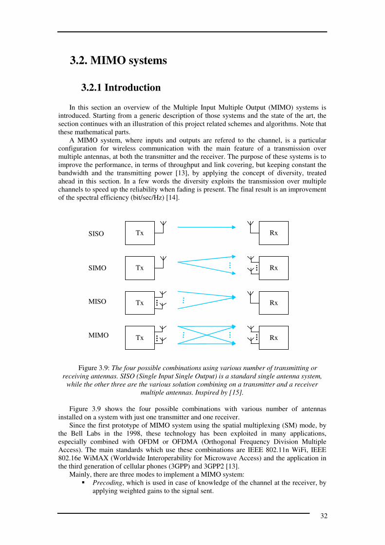
Figure 3.9: The four possible combinations using various number of transmitting or
receiving antennas. SISO (Single Input Single Output) is a standard single antenna system,
while the other three are the various solution combining on a transmitter and a receiver
multiple antennas. Inspired by [15].
Figure 3.9 shows the four possible combinations with various number of antennas
installed on a system with just one transmitter and one receiver.
Since the first prototype of MIMO system using the spatial multiplexing (SM) mode, by
the Bell Labs in the 1998, these technology has been exploited in many applications,
especially combined with OFDM or OFDMA (Orthogonal Frequency Division Multiple
Access). The main standards which use these combinations are IEEE 802.11n WiFi, IEEE
802.16e WiMAX (Worldwide Interoperability for Microwave Access) and the application in
the third generation of cellular phones (3GPP) and 3GPP2 [13].
Mainly, there are three modes to implement a MIMO system:
� Precoding, which is used in case of knowledge of the channel at the receiver, by
applying weighted gains to the signal sent.
Tx
Rx
Tx
Rx
Tx
Rx
Tx
Rx
SISO
SIMO
MISO
MIMO

33
� Spatial multiplexing, which transmit the data split on the multiple antennas, it
does not uses any channel knowledge at the transmitter.
� Diversity Coding, which does not have any knowledge about the channel at the
transmitter, send the data with redundancy in various time and with alternate
phases.
In this report, the blind techniques only are considered, focusing on the spatial
multiplexing’s channel matrix inversion and the space-time block coding.
3.2.2 The concept of diversity
Diversity is a technique to improving the throughput by transmiting data through two or
more channels with different features [16]. This multiple channel allows to avoid the
degradations introduced by the multipath fading, by transmitting the data streams with
repetition, but different phases, so at the receiver is possible to combine these correlated
informations. The main types of diversity schemes are [17]:
� Time diversity, which consists in the transmitting the same signals at different
time consecutively, but with different features (i.e. changing the phase). Note that
the concept of time diversity does not include the MIMO.
� Frequency diversity, which transmits the signal using various carrier frequencies
in order to exploit various channel frequency-slots, or spreading the whole
spectrum. A typical example is the OFDM modulation with interleaving and error
correction.
� Space diversity, which is the transmission of the same data stream on various
antennas, then through different channels, and it is strictly related to the MIMO
schemes (or multiple-cable connections). Moreover, there are two definition of
space diversity depending on the distance of the antennas at the transmitter,
which can be pleced on different base-stations or at one wavelength, respectively
called macro or microdiversity.
� Polarization diversity, which transmits at the same time various versions of the
signal on multiple antennas, which are polarized in different mode.
� Multiuser diversity, which transmits the data from a user selected as the best
between a certain number of receivers, called opportunistic user. This technique
needs a channel estimation at the transmitter, or alternatively at the receiver with
a feedback communication.
� Cooperative diversity, which sends gained signals depending on the information
coming from the distributed antennas which can cooperate to improve the
throughput.
Note that in this report the first three types of diversity are considered, in particular
relatively to the Space-time block coding MIMO mode, which joins the time and space
diversity, and to the OFDM modulation concerning the frequency diversity. In the next
sections the MIMO techniques related to this project are expleined, those that, as
explained in the chapter “problem analysis”, have simpler algorithms in order to reduce
the computational load at the receiver.
3.2.3 Spatial multiplexing
In this section an description of a space diversity technique is explained, the spatial
multiplexing (SM) [16] and [18]. Note that this modality join the concept of diversity with
those of multiple antennas, but just the case of MIMO is treated. This because the basic case
of a MISO-SM differs from the MIMO-SM (with the same number of transmitting antennas)

34
just at the receiver. The peculiarity of the SM mode is the an inversion of the channel matrix
to decode the signal, and this computation [16] and [18], is used for the algorithms explained
in the implementation.
The scheme presented in this section is those shown in Figure 3.10, with two antennas at
both the transmitter and the receiver.
Figure 3.10: The scheme of a MIMO system with two antennas at both the transmitter and
the receiver, and additional white noise. The stream transmitted are split in two following the
Spatial Multiplexing technique.
Figure 3.10 shows a semplified scheme of the system, where the input is a sequence of
complex symbols, indicated with X(t), which on the two antennas is split. x1 and x2 indicate
the two symbols transmitted at the same time interval, while y1 and y2 those received. A white
Gaussian noise is assumed, n1 and n2; the channels are noted as hij, also complex quantities,
where i is related to the number of the receiving antenna and j the transmitting antenna. The
output signal )(ˆ tX is an estimation of the transmitted series.
The signals received on the two antennas are a mixture of the transmitted symbols,
weighted on the different paths of the channel, added to the noise components. (Some of the
following equations for SM mode have been obtained in the algorithm analysis of the first
semester project [19]).
22221122
12121111
nxhxhy
nxhxhy
++=
++= (3.9)
where the received symbols yi are composed by the addition of the multiplication between
the transmitted symbols xj and the channel features hij, and the nise components ni. Moreover,
every component of these equations are defined in the complex domain. Assuming that the
channel follows a Rayleigh distribution and the noise a Gaussian behaviour, the relative
domains are defined as:
( )2,0, hij Ch σΝa ( )2,0, ni Cn σΝa (3.10)
where C means complex domain, and N indicates the normal distribution with mean zero
and variance2
hσ and 2
nσ .
Formula 3.9 can be expressed in matrix notation, compact and extended respectively:
NXHY +×= (3.11)
+
×
=
2
1
2
1
2221
1211
2
1
n
n
x
x
hh
hh
y
y (3.12)
x1
X(t)=[...,x3,x2,x1,...]
x2
TR
AN
SM
ITT
ER
n1
y1
)(ˆ tX
n2 y2
RE
CE
IVE
R
h11
h21
h12
h22
35
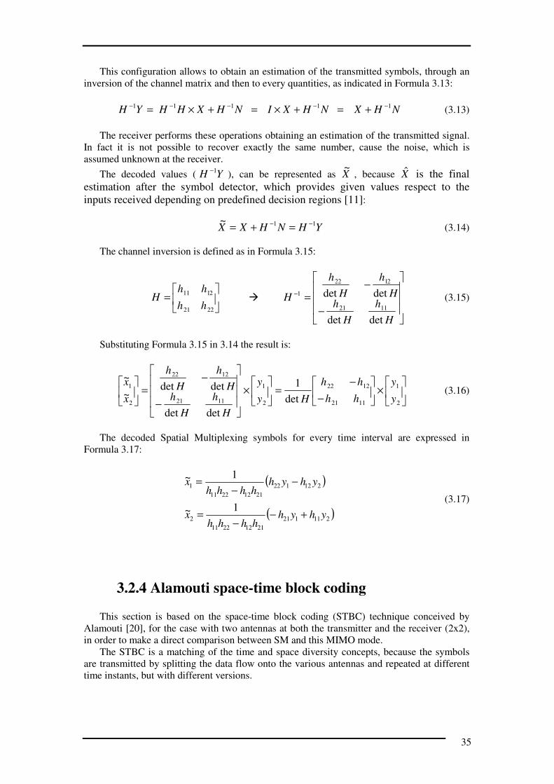
This configuration allows to obtain an estimation of the transmitted symbols, through an
inversion of the channel matrix and then to every quantities, as indicated in Formula 3.13:
NHXNHXINHXHHYH 11111 −−−−− +=+×=+×= (3.13)
The receiver performs these operations obtaining an estimation of the transmitted signal.
In fact it is not possible to recover exactly the same number, cause the noise, which is
assumed unknown at the receiver.
The decoded values ( YH 1−), can be represented as X
~, because X̂ is the final
estimation after the symbol detector, which provides given values respect to the
inputs received depending on predefined decision regions [11]:
YHNHXX11~ −− =+= (3.14)
The channel inversion is defined as in Formula 3.15:
=
2221
2111
hh
hhH �
−
−=−
H
h
H
hH
h
H
h
H
detdet
detdet
1121
2122
1 (3.15)
Substituting Formula 3.15 in 3.14 the result is:
×
−
−=
×
−
−=
2
1
1121
1222
2
1
1121
1222
2
1
det
1
detdet
detdet~
~
y
y
hh
hh
Hy
y
H
h
H
hH
h
H
h
x
x (3.16)
The decoded Spatial Multiplexing symbols for every time interval are expressed in
Formula 3.17:
( )
( )211121
21122211
2
212122
21122211
1
1~
1~
yhyhhhhh
x
yhyhhhhh
x
+−−
=
−−
=
(3.17)
3.2.4 Alamouti space-time block coding
This section is based on the space-time block coding (STBC) technique conceived by
Alamouti [20], for the case with two antennas at both the transmitter and the receiver (2x2),
in order to make a direct comparison between SM and this MIMO mode.
The STBC is a matching of the time and space diversity concepts, because the symbols
are transmitted by splitting the data flow onto the various antennas and repeated at different
time instants, but with different versions.

36
Figure 3.11: The scheme of a MIMO system two by two antennas (2x2), and additional
white Gaussian noise. The data in input X(t) are split in two with repetition, but alterning and
complex conjugating respect to the first time instant.
The scheme of Figure 3.11 shows the 2x2 MIMO system with STBC mode, where the
data in input are split onto two antennas. Note that this block scheme is the semplified version,
as for the SM, that does not specify the mapping and demapping of the symbols. The system
exploit two time intervals to transmit an information redoundant sequence, because at the first
step the top antenna sends x1 and the bottom antenna x2, while at the second time interval the
complex conjugated *
2x− and *
1x respectively. The signals cross the multiple channel hij,
where i receiving antennas and j transmitting antennas, and the received sequence is yit,
where t is the time interval. As in the SM scheme, the shown system by a white Gaussian
noise on the receiving antennas nit is affected, and the estimated information after the symbol
detection is X̂ . The received signals are the combination of the complex products expressed in Formula
3.18 for the two time intervals. (Note that the following equations for the STBC have been
taken or inspired by [19], as for the SM case).
2212222122
2122212121
1211221112
1121211111
nxhxhy
nxhxhy
nxhxhy
nxhxhy
++−=
++=
++−=
++=
∗∗
∗∗
(3.18)
where yit are the received signals on antenna i at the two time intervals and the other
quantities are those defined for Figure 3.11. As for the SM case the generic expression in
matrix notation is those indicated in Equation 3.19, but the extended version needs a complex
conjugation of the lines 2 and 4 of Formula 3.18, so this expression alrady contains these
modifications. In fact, to obtain the extended matrix notation, the expressions related to the
second time instant must be those shown in Formula 3.20.
NXHY +×= (3.19)
*
221
*
222
*
21
*
22
*
121
*
122
*
11
*
12
nxhxhy
nxhxhy
++−=
++−= (3.20)
In this way, the received signals can be represented in extended matrix notation, in
Formula 3.21.
...- x2*, x1
X(t)=[...x3,x2,x1...]
... x1*, x2
TR
AN
SM
ITT
ER
…n12,n11
..y12,y11
)(ˆ tX
…n12,n11 ..y22,y21
RE
CE
IVE
R
h11
h21
h12
h22
37
+
×
−
−=
∗∗
∗∗
22
21
12
11
2
1
2122
2221
1112
1211
22
21
12
11
n
n
n
n
x
x
hh
hh
hh
hh
y
y
y
y
(3.21)
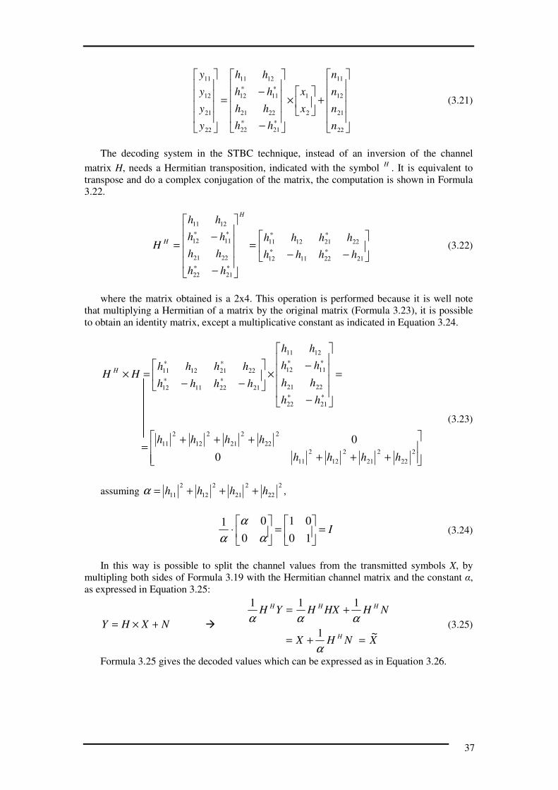
The decoding system in the STBC technique, instead of an inversion of the channel
matrix H, needs a Hermitian transposition, indicated with the symbol H
. It is equivalent to
transpose and do a complex conjugation of the matrix, the computation is shown in Formula
3.22.
−−=
−
−=
∗∗
∗∗
∗∗
∗∗
21221112
22211211
2122
2221
1112
1211
hhhh
hhhh
hh
hh
hh
hh
H
H
H (3.22)
where the matrix obtained is a 2x4. This operation is performed because it is well note
that multiplying a Hermitian of a matrix by the original matrix (Formula 3.23), it is possible
to obtain an identity matrix, except a multiplicative constant as indicated in Equation 3.24.
+++
+++=
=
−
−×
−−=×
∗∗
∗∗
∗∗
∗∗
2
22
2
21
2
12
2
11
2
22
2
21
2
12
2
11
2122
2221
1112
1211
21221112
22211211
0
0
hhhh
hhhh
hh
hh
hh
hh
hhhh
hhhhHH H
(3.23)
assuming 2
22
2
21
2
12
2
11 hhhh +++=α ,
I=
=
⋅
10
01
0
01
α
α
α (3.24)
In this way is possible to split the channel values from the transmitted symbols X, by
multipling both sides of Formula 3.19 with the Hermitian channel matrix and the constant α,
as expressed in Equation 3.25:
NXHY +×= �
XNHX
NHHXHYH
H
HHH
~1
111
=+=
+=
α
ααα (3.25)
Formula 3.25 gives the decoded values which can be expressed as in Equation 3.26.

38
( )
( )222121
*
22121111
*
122
22
2
21
2
12
2
11
2
222221
*
21121211
*
112
22
2
21
2
12
2
11
1
1~
1~
yhyhyhyhhhhh
x
yhyhyhyhhhhh
x
−+−+++
=
++++++
=
(3.26)
In [20] the Alamouti’s STBC mode has been tested and compared with the SISO scheme
and the Maximal-Ratio Receive Combining technique (MRRC) [20], which consists in a
single transmitting antenna and multiple receiving antennas.
Figure 3.12 shows the benefits of the STBC assuming Rayleigh fading channel
transmission and BPSK modulation.
SNR[dB]
Figure 3.12: The bit error rate (BER) behaviour for various possible values of signal to
noise ratio (SNR). Comparison between single and multiple antennas systems transmitting
with a coherent BPSK through a Rayleigh fading channel, from [20].
Note that the comparison in Figure 3.12 is done assuming [20] fixed transmission power,
Rayleigh fading with mutually uncorrelated amplitudes and ideal channel estimation, which
means a perfect knowledge of the channel features at the receiver.
Comparing the various technique it is possible to appreciate the benefit of multiple
antennas systems and in particular it is demonstrated that increasing the number of elements
(antennas) has a proportional improvement of the channel capacity [13, ch.7]. The Alamouti
2x2 is worse than the MRRC 1x4, but from a practical point of view it is better to have as less
antennas on a mobile device as possible, both if the system is composed by transmitter and
receiver or by two transceivers.

39
3.2.5 Alamouti STBC 4x1 with Feedback
This section contains the Alamouti STBC technique applied to system with four
transmitting antennas, and an antenna at the receiver. The focus is on the transmitting scheme,
complicated because a non-orthogonality in the channel matrix calculation. The technique
analyzed in [21], [22] and [23] uses a feedback to limit the effects of this non-orthogonality.
Note that this branch of the MIMO research has been chosen because very actual and it is the
extension of the Alamouti STBC technique which, as indicated in the previous section, is
computationally light respect to the benefits it apports to a telecommunication system [20].
This means that can by a possible way to limit the cost function (area, speed, energy, price) in
the real applications of mobile systems. Note also that the cases of multiple receiving
antennas the computation is the same, except for the channel matrix, moreover the reception
aspect of these cases, in the second part called “Design” is treated.
The scheme considered is a STBC-MIMO as those in Figure 3.11, but with four
transmitting antennas, so four symbols are transmitted with repetition alternatively on the
antennas, with different versions at four time intervals, as shown in Figure 3.13.
Figure 3.13: The scheme of a MIMO 4x1, transmitting in Alamouti mode in four time
intervals and feedback. The kind of back transmission is not treated.
As indicated in Figure 3.13, the symbols are transmitted in different versions as in
Formula 3.27. Note that this section’s formulas are given and inspired by [22].
−−
−−
−−=
1234
*
2
*
1
*
4
*
3
*
3
*
4
*
1
*
2
4321
xxxx
xxxx
xxxx
xxxx
X (3.27)
where the columns indicate the symbols transmitted on the antennas, and the rows the
time instants. The signal received is those expressed in Formula 3.28, where Y is the matrix
with the second and the third rows already complex conjugated.
... x4, x3*, x2*, x1
...- x3, x4*,- x1*, x2
X(t)=[.. x5,x4,
x3,x2,x1...]
...- x2,- x1*, x4*, x3
... x1,- x2*,- x3*, x4
TR
AN
SM
ITT
ER
h1
h2
h3
h4
..y2,y1
)(ˆ tX
…n2,n1
feedback
RE
CE
IVE
R

40
4413223144
*
34
*
23
*
12
*
41
*
3
*
3
*
24
*
33
*
42
*
11
*
2
*
2
1443322111
nxhxhxhxhy
nxhxhxhxhy
nxhxhxhxhy
nxhxhxhxhy
++−−=
+++−−=
++−+−=
++++=
(3.28)
which in matrix notation is those in Formula 3.29.
NXHY +×=
+
×
−−
−−
−−=
4
*
3
*
2
1
4
3
2
1
1234
*
2
*
1
*
4
*
3
*
3
*
4
*
1
*
2
4321
4
*
3
*
2
1
n
n
n
n
x
x
x
x
hhhh
hhhh
hhhh
hhhh
y
y
y
y
(3.29)
The STBC decoding computes a Hermitian transposition at the receiver, so Expression
3.30 shows this complex conjugation of the transposition of the channel matrix.
−−
−−
−−
=
−−
−−
−−=
*
123
*
4
*
214
*
3
*
341
*
2
*
432
*
1
1234
*
2
*
1
*
4
*
3
*
3
*
4
*
1
*
2
4321
hhhh
hhhh
hhhh
hhhh
hhhh
hhhh
hhhh
hhhh
H
H
H (3.30)
The purpose of the hermitian channel matrix is to obtain an identity if multiplied by the
original H, except a multiplicative factor, but in the cases of MIMO/MISO with thre or more
transmitting antennas this multiplication does not give a pure identity, as indicated in
Formula 3.31 and 3.32.
−
−=
=
−−
−−
−−×
−−
−−
−−
=×
αβ
αβ
βα
βα
00
00
00
00
1234
*
2
*
1
*
4
*
3
*
3
*
4
*
1
*
2
4321
*
123
*
4
*
214
*
3
*
341
*
2
*
432
*
1
hhhh
hhhh
hhhh
hhhh
hhhh
hhhh
hhhh
hhhh
HHH
(3.31)
assuming 2
4
2
3
2
2
2
1 hhhh +++=α and ( )*
324
*
1Re2 hhhh −⋅=β .
IIHH H ≠=
−
−=
~
100/
01/0
0/10
/001
1
αβ
αβ
αβ
αβ
α (3.32)

41
So the decoding processing, by the quantity β/α is affected, and the values are defined in
Expression 3.33.
NHXINHHXHYHXHHHH
αααα
1~111~+⋅=+== (3.33)
In order to reduce this factor β/α, the technique proposed in [22] provide a calculation of
γ, a factor similar to β but with a difference in a sign, in Expression 3.34.
( )*
32
*
41Re2 hhhh −−⋅=γ (3.34)
so comparing the factors β with γ, the smaller value determinates the feedback to send at
the transmitter:
� if β < γ, the transmitter sends the symbols X indicated in Formula 3.27;
� if β > γ, the symbols are transmitted in a different version, called X and defined
in Formula 3.35.
−−−
−−−
−−−
−
=
1234
*
2
*
1
*
4
*
3
*
3
*
4
*
1
*
2
4321
xxxx
xxxx
xxxx
xxxx
X (3.35)
The second modality of transmission indicated in Formula 3.35 differs only on the first
column respect to X, corresponding to the first antenna.
Transmitting one bit in feedback is possible to reduce the interference due to the non
othogonality of the channel matrix product, then this technique in the quasi-orthogonal STBC
(QO-STBC) is classified [21], [22] and [23].
3.3. WMAN IEEE 802.16
In this section a short description of the physical layer of the IEEE 802.16 with MIMO
STBC is given, considering a Matlab Demo implementation [24] and [26].
The IEEE 802.16 is the telecommunication standard on which the Worldwide
Interoperability for Microwave Access (WiMAX) [24] and the Wireless Metropolitan Area
Network (WMAN) [25], [27] are based. They are wireless technologies which provides high
bit rate [24] to the system. In particular this report on the IEEE 802.16d-2004 is focused, even
if there are other versions later, as the last IEEE802.16i [25] which is more advanced. This
choice because those versions treat the multiple access (OFDMA), not considered in this
project.
Figure 3.14 shows the scheme of the Simulink implementation of the Standard IEEE
802.16d [24] and [26], which transmit using an OFDM modulation and a MISO 2x1 system.
Note that the work proposed in the next chapters, is based on this scheme, in particular
focusing on the multiple antenna section.

42
Figure 3.14: The Simulink scheme of the IEEE 802.16d Standard with STBC-MISO 2x1.
On the top in blue the input data source and the transmitter blocks are shown, on the right
the multiple channel (MISO) affected by Additive White Gaussian Noise (AWGN); on the
bottom the receiver. Image from [24] and [26].
Figure 3.14 shows the WMAN Physical Layer Simulink implementation for the standard
IEEE 802.16d [24] and [26], where the blue blocks represent the architecture of the
transmission system, the light green the system to manage the modulations and the Forward
Error Correction (FEC). In yellow the displays (SNR, BER, number of errors and transmitted
bits) and in brown the setting blocks. On the top there are the data source and the transmitter,
on the right the channel MISO model with an Additive White Gaussian Noise AWGN, finally
on the bottom the receiver. Note that in this model the communication works with the
equivalent baseband, because the Radio Frequency (RF) implementation needs more
powerful test environments than Matlab Simulink.
The transmission chain is composed by:
� Random Data Source, which provide random bit in input that simulate the
downlink of the WMAN system. It generates bursts consisting of a certain
number of OFDM symbols.
� Forward Error Correction (FEC), which is developed by a convolutional code
(CC) inside a Reed-Solomon code (RS).
� Data interleaver, which associates the coding to a certain number of subcarriers.
� Modulation bank, which by BPSK, QPSK, 16-QAM and 64-QAM modulations
schemes is composed.
� OFDM transmission, using 192 sub-carriers, 8 pilots signals, 256-point Fast
Fourier Transforms and cyclic prefix that can be changed in the length.
� Space-Time Block Coding, which uses the Alamouti transmission scheme.
� Burst preamble, which is composed by a preamble long a single OFDM symbol.
This symbol preamble is trasmitted from both the antennas.
� MISO fading channel, which follows a Rice behaviour and with AWGN. In this
way it is possible to decode by STBC.
� Diversity combiner, at the receiver allows the OFDM demodulation and the
channel estiamtion by using the preambles.

43
� STBC demodulator, deinterleaver, Viterbi and Reed-Solomon decoders.
The scheme provides an estimation SNR implemented by an adaptive rate control, which
can vary dynamically the modulation depending on the condition of the channel. The
various possible modulations are those indicated in Table 3.1.
RateID Modulation and RS-CC rate
0 BPSK 1/2
1 QPSK 1/2
2 QPSK 3/4
3 16-QAM 1/2
4 16-QAM 3/4
5 64-QAM 2/3
6 64-QAM 3/4
Table 3.1: The modulations and RS-CC rates possible, with the relative RateID, from [24]
and [26].

44

45
Part II
Design

46

47
Figure 4.0: The Rugby Meta-model adapted to this report, the inital idea.
4. Initial Idea
In this chapter the initial point of the project is explained. The idea, in fact, is the first step
emphasized on the Rugby methodology scheme shown in Figure 4.0, and it consists in a
mixing between OFDM and MIMO systems. The four domains are defined as:
� Computation: algorithms of MIMO modes, FFT and OFDM calculations.
� Communication: Matlab and hardware implementation.
� Data: transmission of OFDM symbols on multiple channel.
� Time: not specified.
Note that the list is not detailed because the initial idea does not require specific
information about the system to implement, especially in the time domain.
The idea is at the beginning of the Time and Abstraction lines as indicated in Figure 4.0,
that means the first step of the project working on the highest abstraction level.
Chapter 4 contains two sections, the initial problem, which indicates a short comment
about the state of the art with the question at the base of the project, and second the solution
proposed to answer at this request.
4.1. The problem
The lasts WiMAX systems are already based on multiple antennas communication, and in
particular using the Spatial Multiplexing mode, as indicated in section 3.3. Starting from
these real systems and from the prototypes implemented in the last years, the researchers try
to propose new solutions which can improve the features, in particular speed up the
throughput. The purpose of the project described in this report is to propose a new
architecture combining existing technique, studing the feasibility and analizing the partial
results in order to obtain a hardware implementation. So the development flow must answer
to a question:
“what type of algorithmic improvements can be used to increase the spectral efficiency of an
OFDM/MIMO receiver, while maintaining its HW feasibility?”

48
4.2. Proposed solution
The solution proposed is a combination of OFDM and MIMO systems. Note that this is
the first domain of the A3 model shown in section 2.1. In particular the idea is to use the
Alamouti’s STBC [20] and the Spatial Multiplexing modes in order to extend these theory to
real applications. The work can be divided in two sub-parts :
� Algorithms, where these MIMO and so called extended-MIMO techniques are
analyzed, improved and implemented by software. The analysis includes the
mathematical computations maintaing various architectural solutions, in order to
compare the results obtained by the software simulations and chose the best for
the hardware implementation.
� Architecture, where the best algorithmic solution chosen is developed, first
through software simulators and finally on hardware. The last step is to test and
verify the system implemented.
Note that all the precise information about the solution proposed in this section and the
developing environment, in the next chapter 5 “Constraints and Requirements” are explained.

49
Figure 5.0: The Rugby Meta-model adapted to this report, Constraints and Requirements.
5. Constraints and Requirements
This chapter contains the starting constraints and requirements of the project. This step
consists in the specification of the main limitations and targets as those shown in Figure 5.0,
the Xilinx FPGA series Virtex 5 and MISO/MIMO systems 2x2, 4x1 and 4x4. The domains
of the Rugby Meta-Model are defined as:
� Computation: algorithms of Alamouti and Spatial Multiplexing and equivalent
baseband signals considered. Simulink blocks and Matlab operations are
performed.
� Communication: architecture of the system defined as one transmitter and one
receiver, with a wireless Rayleigh channel. The main internal blocks of the
transmitter are the mapper (for the modulation bank) the MISO/MIMO
combinator and the OFDM modulator. The receiver contains the OFDM
demodulator, the channel estimator and MISO/MIMO decoder, and the
demapping block. The operators are provided by the simulation environment,
which is composed by the computer softwares Matlab, Simulink and System
Generator for DSP, and the operators/interfaces of the co-simulation test
environment, which remain the same but includes the FPGA board.
� Data: transmission by the BPSK, QPSK, 16-QAM and 64-QAM modulations,
redoundancy in the transmission provided by the MISO/MIMO modes. The
transmitted data are affected by Rayleigh fading and white Gaussian noise.
Moreover, at the receiver, there is an error introduced by the channel estimation,
which provides not ideal values. Note that there are no indications about the data
path of the system.
� Time: causality, minimizing the execution time. The transmitter and the receiver
are perfectly synchronized.
Note that the list indicated is more detailed but still generic, because at this point it is not
possible to define precisely any technical features of the system. Anyway this chapter gives a

50
global description of the main components, indicating the the abstraction level is step by step
reducing as shown in Figure 5.0.
Chapter 5 is divided by three sections. The first contains the cost function, which is an
indication on the design trend in terms of metrics, while the second section lists the initial
assumptions, adding more details for the system implementation. Finally a short description
of the tools used in the project for developing and simulating, after a sub-section about the
hardware platform and at the end of the chapter a generic overview on the environment used
for the final tests.
5.1. Cost function
The development of every project must satisfy a number of constraints in order to
characterize the design flow and justify the choice during the implementation. Very often, in
the field of signal processing, there are many trade-off that force the designer to make choices.
In this way, the cost function must be minimized and the constraints fullfilled, a trend that
must be followed to obtain a consistent project.
This project case the metrics considered for the cost function are:
� Execution time, which indicates the time needed by the system to process its
computation. This metric is related to the longest path of the implementation and
the working frequency of the hardware platform. The execution time is
considered because in a telecomunication system the reactivity is fundamental,
especially if the channel features change very often;
� Area, which consists in the resources occupation of the system on the hardware.
Minimize this parameter is necessary because the hardware components are
limited.
( )AtfC ,= (5.1)
In Formula 5.1 the cost function for this project is shown, where t is the execution time
and A is the area. Note that these two metrics are often in a trade-off, so in these cases a
choice must be taken. For example, the implementation of an algorithm using an hardware
embedded processor can limit the number of resources, because the flow of sequential
instructions by the memory-ALU-register architecture, but on the other hand the time needed
to perform the computation is high comparing to a parallel execution. This is the case of a
FPGA implementation, where the operations can be executed in less time and in parallel, but
employing a higher number of resources.
There are also others metrics that can be considered, as price, energy consumption,
easiness, that are not directly treated in this project, even if sometimes the choices implicitly
include them. So in the report these aspect are discussed.
5.2. Assumptions
A telecommunication wireless system working in a real environment, is affected by noise,
multipath fading, and many other degradations with different entity. These imply the
engineering method of the environment modeling, which consists in a mathematical
semplification of the communication.
In this project the assumptions defined are:
� OFDM-MISO/MIMO, which indicates the generic delimitation that the system
must include the orthogonal modulation by applying multiple antennas system.
� BPSK, QPSK, 16-QAM, 64-QAM, are the modulations that must be implemented
for the pre-mapping of the data, which can be singularly selected depending on

51
the transmission features (SNR, channel behaviour). In particular the
convolutional codes that can be selected for the various modulations are: BPSK
½, QPSK ½, QPSK ¾, 16-QAM ½, 16-QAM ¾, 64-QAM ²/3, 64-QAM ¾.
� Alamouti’s STBC/SM, which are the modes to be implemented in the various
solution designed. In the detail, the soutions must consider the Alamouti scheme
for the MIMO 2x2, and Alamouti or SM for the MISO 4x1 and MIMO 4x4.
� Target hardware, which is the Xilinx Field Programmable Gate Array (FPGA)
Virtex 5 xc5vsx50t, that is put on the platform board ML506 [28] and [29]. This
hardware must process one of the algorithms implemented in software (listed in
the previous point).
� Rayleigh channel, which indicates the model of multipath fading of the wireless
channel. In particular the time-varying gain of the channel have a Rayleigh
distribution. There is no line-of-sight, and the features of the channel are not
changing during a STBC cycle (equal to i time intervals, where i is the number of
receiving antennas).
� AWGN, which is the only noise considered, that is added to the receiving
antennas during the communication, it follows a Complex Normal distribution.
� Not singularity of the channel complex matrix (determinant different from zero),
which allows the inversion/pseudoinversion.
� Channel estimation, which provides the values for the computation at the receiver,
affecting the system by non-ideality.
� IEEE 802.16d WMAN Physical Layer Simulink Demo, which is the standard
implementation based on [24], in [26], described in section 3.3, to use as base for
this project.
� Perfect synchronization between the transmitter and the receiver.
� No Radio Frequency (RF). The system does not include the RF part because the
simulator ar not power enougth to process high frequency (microwaves range), so
the signal transmitted on the channel is the equivalent in baseband.
� Matlab and Simulink, program environments for the simulations and HW/SW co-
simulation, using the Xilinx libraries and the tool Xilinx System Generator for the
VHDL synthesis and bit-stream file.
5.3. Matlab, Simulink and System Generator
Matlab [30] is a software for technical computation, which provides an own
programming language and a platform for the implementation of programs, as shown in
Appendix A, Figure 5.1. This program is used for the settings files needed by the Simulink
systems, and also to test and simulate functions relative to some blocks of Simulink. Simulink
is a tool which consists in a graphic platform where it is possible to put and connect various
functional blocks. It is based on the Matlab software, so these blocks are just graphic
representation of predefined functions. Simulink is very useful to implement complex
systems as those in this project, because by setting the internal block parameters is possible to
obtain the functionality required. Moreover, it is possible to program directly Xilinx FPGA
through provided compilers. In fact, there are special libraries that provide Simulink blocks
synthetizable directly into hardware components. These compiler is called Xilinx System
Generator for DSP [31], which is able to convert these Xilinx Matlab functions into VHDL
code and in bit-stream files, allowing the direct programming of the FPGA. In particular,
System Generator for DSP (SysGen) provides design blocks which are, from an architectural
point of view, more basic than those from the standard libraries of Simulink. Moreover,
SysGen allows to specify the data path (in fixed point notation) of each block, provide test
bench simulation, VHDL code generation and co-simulation (explained in section 5.3.2).
Given the target hardware a Xilinx FPGA, this tools have been chosen because
recommended by the company to “easily” design an integrated system. Moreover, this

52
software trilogy allows the HW/SW co-simulation, a functionality explained in sub-section
5.3.3. Figure 5.2 and 5.3 in Appendix A, show the Simulink and System Generator
environment, respectively.

53
Figure 6.0: The Rugby Meta-model adapted to this report, System Analysis and Modeling.
6. System Analysis and Modeling
In chapter 6 the MISO/MIMO system analysis and the model of this project are explained.
This is the third step of the applied Rugby methodology scheme in Figure 6.0. The system
analysis consists in an overview of the algorithms which are used in the software/hardware
implementation. The domains of the Rugby Meta-Model for this chapter are:
� Computation: the IEEE 802.16d scheme considered contains various algorithms,
for the data computation, as the random source, the modulation bank, the OFDM
symbol building, the OFDM modulation, the demodulation and the error
correction. These computations are equal to the Simulink demo. The remaining
algorithms, about the MIMO encoder and combiner, are respectively modified
and replaced by the new solutions. In particular there are two new decoding
techniques which are explained in the details, the channel inversion/pseudo-
inversion and the subtractive method. Moreover these two algorithms, to the
cases of 4x1 and 4x4 systems are applied.
� Communication: in this chapter the architecture analysis goes more in the deep,
and the main blocks of the WMAN scheme are shown. Some blocks are kept
unmodified, and those performing the MISO/MIMO-OFDM are modified or
replaced. In particular, the combiner is redesigned using two new approaches. In
this chapter, the algorithm operations of these techniques are analyzed. The
operations are defined in the complex domain, as multiplications, divisions,
additions and subtractions.
� Data: the system transmits symbols. Each value considered is a complex
quantity, without specification about the accuracy. The wireless channels are
modeled as Rayleigh distribution and the noise at the reception follows a
Gaussian behaviour.
� Time: the time parameters are those related to the Alamouti STBC with four
transmitting antennas. In fact, groups of 4 symbols are transmitted on the 4
terminals in 4 time instants.

54
The bottom part of Figure 6.0 indicates the timing and abstraction level of the
implementation. The analysis treats internal blocks, showing the algorithms of those
implemented in this project.
Note that the WMAN system at the basis of this project is just an instrument to perform
the MISO/MIMO techniques applied to OFDM modulation. The work focuse on these parts,
and in particular on the receiver. In fact, the target of this project is the MISO/MIMO
combiner analysis and its hardware implementation.
Chapter 6 consists on two sections, where the first gives a global description of the basic
WMAN system by focusing on the blocks which are developed. The second section treats the
various algorithms for the MISO/MIMO combiners, where two new techniqes are proposed
and analyzed in the detail. A short discussion on the various decoding noise is done, just to
have a qualitative indication about the quality of the two techniques.
6.1. Global description
The telecommunication system implemented in this project is based on the Simulink
Demo [26] IEEE 802.16d [24] standard and is extended with the MISO/MIMO section. In
particular the project focuses on different parts, first regarding the software simulations and
second about the hardware implementation and co-simulation. The work done for the
simulations treats the part MISO/MIMO encoder and decoder, for the various cases indicated
in section 5.2, and the channel model. The work done on the hardware concerns just the
receiver side (decoder) and in particular considering the MIMO mode which has best
simulation results between those treated.
Figure 6.1: The blocks where this project is focused. The IEEE 802.16d is based on a OFDM-
MIMO system with a generic number of antennas for both transmitter and receiver. The
green block is those implemented on hardware and the green plus blue blocks those
developed for the software simulations.

55
About the hardware implementation, the receiver side has been choosen because more
interesting and complex in terms of trade-off between computation load and physical
constraints, such as area occupation and energy consumption.
Figure 6.1 shows the part where the work is focused, based on the Simulink demo
WMAN with generic MIMO system. The blocks in blue and the greeen are those
implemented for the MISO/MIMO encoders defined in section 5.2, while for the hardware
just the green block is developed. In Figure 6.1 the number of antennas is not specified, as the
number of OFDM transmitters and receivers. The AWGN has been indicated with one block,
but the contribution on each receiving antennas is fully independent.
6.2. Algorithms analysis
This section contains the various algorithms implemented in this project, with a
mathematical description of two new approaches for the MISO/MIMO reception. In fact, as
explained in section 3.2, the using of more than three transmitting antennas causes non
orthogonality (that gave the name of QO-MIMO), and the constraints are 2x2, 4x1 and 4x4.
The theory relative to the 2x2 has already treated in section 3.1, so it is just applied to the
Simulink scheme. Anyway, the transmission with 4x1 and 4x4 antennas introduced in sub-
section 3.2.5 needs to transmitt one bit (or more [22]) in feedback. In order to avoid that, this
section shows two new techniques to combine the received data reducing the effect of the non
orthogonality in the channel matrix: one is based on a channel inversion as the Spatial
Multiplexing combiner, but keeping the STBC transmission mode; the second is a classic
STBC mode but with a subtractive technique. Note that these two algorithms can work on
both 4x1 and 4x4 antennas systems.
6.2.1 Channel inversion combiner 4x1
The system considered in the following sub-sections consists in the same transmitter of
those presented in section 3.2.5, with four antennas transmitting in Alamouti STBC mode.
Anyway the combiner at the receiver is based on a different computation, with channel
inversion as those of the Spatial Multiplexing mode. Figure 6.2 shows the system 4x1 in
STBC mode, which differs from Figure 3.13 in the missing feedback.
Figure 6.2: The scheme of a MISO 4x1, transmitting in Alamouti STBC mode in four time
intervals. From Figure 3.13.
... x4, x3*, x2*, x1
...- x3, x4*,- x1*, x2
X(t)=[.. x5,x4,
x3,x2,x1...]
...- x2,- x1*, x4*, x3
... x1,- x2*,- x3*, x4
TR
AN
SM
ITT
ER
h1
h2
h3
h4
..y2,y1
)(ˆ tX
…n2,n1
RE
CE
IVE
R

56
The symbols transmitted are those in Formula 6.1, as indicated in Formula 3.27, inspired
by [22].
−−
−−
−−=
1234
*
2
*
1
*
4
*
3
*
3
*
4
*
1
*
2
4321
xxxx
xxxx
xxxx
xxxx
X (6.1)
The multiplication between the Hermitian channel matrix and the original H, as indicated
in Formula 3.31 and reproposed in Equation 6.2, gives a matrix not diagonal.
−
−=
−−
−−
−−×
−−
−−
−−
=×
αβ
αβ
βα
βα
00
00
00
00
1234
*
2
*
1
*
4
*
3
*
3
*
4
*
1
*
2
4321
*
123
*
4
*
214
*
3
*
341
*
2
*
432
*
1
hhhh
hhhh
hhhh
hhhh
hhhh
hhhh
hhhh
hhhh
HH H
(6.2)
assuming 2
4
2
3
2
2
2
1 hhhh +++=α and ( )*
324
*
1Re2 hhhh −⋅=β .
So this non orthogonality is translated in a non ideal matrix in Formula 6.3 (reproposed
from Formula 3.32).
IIHH H ≠=
−
−=
~
100/
01/0
0/10
/001
1
αβ
αβ
αβ
αβ
α (6.3)
This error β/α affects the reception and the classical Alamouti’s decoding does not work
if it want avoid the feedback as in Formula 6.4 (from Equation 3.33).
NHXINHHXHYHXHHHH
αααα
1~111~+⋅=+== (6.4)
Starting from this point, the idea is to change the computation and force the receiver to
have a pure identity in the decoding computation. This can be implemented as indicated in
Formula 6.5, introducing an unknown matrix M.
IMHH H = (6.5)
where this new matrix is put in the multiplication to avoid the non-orthogonality and the
multiplicative factor 1/α. The computation becames those in Formula 6.6.
MNHXMNHMHXHMYHX HHHH +=+==~
(6.6)
The unknown matrix M is calculated in the next Formulas 6.7-6.10, starting from
Equation 6.5.
IHMHHH HHH 11 −− = (6.7)

57
I
Multiplying Formula 6.5 from the left (of course on both sides) by the inversion of the
Hermitian channel matrix 1−HH , Formula 6.8 is obtained. Note that the inversion is possible
only for squared not singular matrixes, so this computation is valid just for the 4x1. In fact,
for the 4x4 the estimated channel matrix H is rectangular with 16 rows and 4 columns, but
this aspect in sub-section 6.2.4 is treated.
1−= HHMH (6.8)
Multiplying Formula 6.8 by the channel inverted matrix 1−H from the right side,
Equation 6.9 is obtained.
111 −−− = HHMHH H (6.9)
I
The value of matrix M is then indicated in Formula 6.10.
11 −−= HHM H (6.10)
So combining Formula 6.10 and the first part of 6.6, the final computation for the
decoding system is those shown in Equation 6.11.
NHXYHYHHHMYHX HHH 1111~ −−−− +==== (6.11)
which shows how it is possible to decode the signal by using a simple channel inversion,
as for a standard Spatial Multiplexing 2x2 system. However note that the MIMO mode used
is not a SM, because the transmitter remains the standard STBC with four antennas.
The signal decoded in extended version is indicated in Formula 6.12.
×
=
×
−−
−−
−−=
−
4
3
2
1
16151413
1211109
8765
4321
4
3
2
1
1
1234
*
2
*
1
*
4
*
3
*
3
*
4
*
1
*
2
4321
4
3
2
1
det
1
~
~
~
~
y
y
y
y
qqqq
qqqq
qqqq
qqqq
H
y
y
y
y
hhhh
hhhh
hhhh
hhhh
x
x
x
x
(6.12)
where det H is those indicated in Formula 6.13.
det H =
( ) 2
3
2*
2
2*
4
2
1
2
4
2
3
2
4
2
2
2
3
2
2
2
1
43
*
2
*
14
*
32
*
1
*
4
*
321
*
43
*
21
4
4
4
3
4
2
4
1
22222
2222det
hhhhhhhhhhh
hhhhhhhhhhhhhhhhhhhhH
−−++++
++++++++=
(6.13)
And the values of the matrix composed by the elements qw, where w is a number from 1
to 16 indicating row and column, are calculated with the formula in reference [34]. In
Formula 6.14 are reported just few of these values to give an indication of the order of
magnitude.

58
( )( )( )
( ) 4
2*
13
*
2
*
1
*
32
*
1
2
4
2
3
2
2
*
44
3
2
242
*
1
*
421
2
4
2
3
2
133
*
2
2
3
*
43143
*
1
2
4
2
2
2
122
1
2*
4
*
4
*
32
*
43
*
2
2
3
2
2
2
1
*
11
hhhhhhhhhhhhq
hhhhhhhhhhhhq
hhhhhhhhhhhhq
hhhhhhhhhhhhq
−++++=
+−−++−=
+−−++−=
−++++=
(6.14)
With the channel inverted matrix it is possible to calculate the decoded signal, which are
the four decoded symbols.
However the qw values are used also for the noise calculation, even if in the practice is not
possible without noise estimation. Anyway it is useful to calculate mathematically these
values just to have an indication of the decoded noise entity, indicated in Formula 6.16.
NHW1−= (6.15)
where W is the decoding error due to the noise.
( )443322111det
1nqnqnqnq
Hw +++= (6.16)
In Formula 6.16 the decoding error w1 of the first decoded symbol is indicated. The other
three errors are not reported, but them values have the same order of magnitude.
6.2.2 Subtractive combiner 4x1
In this sub-section the second new approach is presented, the subtractive combiner. Note
that the transmitter with four antennas is the same of those presented in section 3.2.5 and
6.2.1. The MISO mode is Alamouti STBC and at the receiver the first computation is the
same as in a classic STBC combiner, but the second part consists in a subtractive
computation. The transmission considered scheme is the same shown in Figure 6.2, and the
computation is those defined in sub-section 3.2.5. The decoded symbols are indicated in
Formula 6.17 (which is equal to Equation 3.33).
NHXIYHXHH
αα
1~1~+⋅== (6.17)
where 2
4
2
3
2
2
2
1 hhhh +++=α and
IIHHH ≠=
−
−=
~
100/
01/0
0/10
/001
1
αβ
αβ
αβ
αβ
α (6.18)
where ( )*
324
*
1Re2 hhhh −⋅=β and the result is not an identity matrix .

59
−−
−−
−−
=
*
123
*
4
*
214
*
3
*
341
*
2
*
432
*
1
hhhh
hhhh
hhhh
hhhh
HH (6.19)
as indicated in Formula 3.32 and Formula 3.30 respectively.
Formula 6.17 can be extended as shown in Equation 6.20, where the decoded noise is
kept in reduced notation to semplify the representation.
×+
×
−
−=
=
×
−−
−−
−−
=
4
*
3
*
2
1
4
3
2
1
4
*
3
*
2
1
*
123
*
4
*
214
*
3
*
341
*
2
*
432
*
1
4
3
2
1
1
100/
01/0
0/10
/001
1
~
~
~
~
n
n
n
n
H
x
x
x
x
y
y
y
y
hhhh
hhhh
hhhh
hhhh
x
x
x
x
H
α
αβ
αβ
αβ
αβ
α
(6.20)
Formula 6.20 is reproposed as in Equation 6.21.
×+
⋅+
⋅−
⋅−
⋅+
=
+++
−+−
−−+
+−−
=
4
*
3
*
2
1
14
23
32
41
4
*
1
*
32
*
231
*
4
4
*
2
*
31
*
241
*
3
4
*
3
*
34
*
211
*
2
4
*
4
*
33
*
221
*
1
4
3
2
1
1
/
/
/
/
1
~
~
~
~
n
n
n
n
H
xx
xx
xx
xx
yhyhyhyh
yhyhyhyh
yhyhyhyh
yhyhyhyh
x
x
x
x
H
α
αβ
αβ
αβ
αβ
α (6.21)
In the subtractive technique a new notation is introduced, in order to semplify the
calculation, proposed in Formula 6.22.
NH
D
C
B
A
n
n
n
n
H
yhyhyhyh
yhyhyhyh
yhyhyhyh
yhyhyhyh
xx
xx
xx
xx
HH
αααα
αβ
αβ
αβ
αβ
1111
/
/
/
/
4
*
3
*
2
1
4
*
1
*
32
*
231
*
4
4
*
2
*
31
*
241
*
3
4
*
3
*
34
*
211
*
2
4
*
4
*
33
*
221
*
1
14
23
32
41
−
=
×−
+++
−+−
−−+
+−−
=
⋅+
⋅−
⋅−
⋅+
(6.22)
where the decoded noise is subtracted from Equation 6.21, while A, B, C and D are the
four lines of the product YHH .
To perform the subtractive technique it is necessary to introduce a new vector X , defined
in Formula 6.23. This vector includes the noise vector N , allowing the real implementation to
decode without noise estimation. However this quantity introduce decoding errors that can
not be neglected. To have an indication on the order of magnitude of this noise vector, it is
separately calculated.

60
NH
xx
xx
xx
xx
x
x
x
x
xx
xx
xx
xx
H
α
αβ
αβ
αβ
αβ
αβ
αβ
αβ
αβ
1
/
/
/
/
~
~
~
~
/
/
/
/
14
23
32
41
4
3
2
1
14
23
32
41
+
⋅+
⋅−
⋅−
⋅+
=
=
⋅+
⋅−
⋅−
⋅+
(6.23)
=
+++
−+−
−−+
+−−
=
⋅+
⋅−
⋅−
⋅+
D
C
B
A
yhyhyhyh
yhyhyhyh
yhyhyhyh
yhyhyhyh
xx
xx
xx
xx
αα
αβ
αβ
αβ
αβ
11
/
/
/
/
4
*
1
*
32
*
231
*
4
4
*
2
*
31
*
241
*
3
4
*
3
*
34
*
211
*
2
4
*
4
*
33
*
221
*
1
14
23
32
41
(6.24)
Note that the vector X is taken as result of the decoding process, and it differs from X~
.
Formula 6.24 shows that there are correlations between the various lines, and can be
reproposed as an system of equation, in Formula 6.25.
+−=
+=
+=
+−=
α
βα
βα
βα
β
Dxx
Cxx
Bxx
Axx
1
4
2
3
3
2
4
1
(6.25)
By solving the system of equation in Formula 6.25, the decoded values are obtained,
which are written in Equation 6.26.
Λ−
Ψ=
Λ+
Ψ=
Λ+
Ψ=
Λ−
Ψ=
ADx
BCx
CBx
DAx
4
3
2
1
where
−=Ψ
2
2
1α
βα and
−=Λ
2
22
1α
β
β
α (6.26)
The mathematical expression of the noise vector is reported in the next formulas.
==
4
3
2
1
111
w
w
w
w
WNH H
ααα (6.27)
where W is the weighed noise vector. These noise components are added to the received
signals. It is possible to calculate these values, called ei, where i indicates the receiving
antenna. The results are shown in Formula 6.28.

61
Λ−
Ψ−=→
Λ+
Ψ−=→
Λ+
Ψ−=→
Λ−
Ψ−=→
14
44
23
33
32
22
41
11
wwex
wwex
wwex
wwexvaluedecodedonnoise
(6.28)
The noise vector of the channel inversion combiner has equations completely different
respect to those of the subtractive decoder. The two formulas contain the same variables, but
the mathematical computation of the first case needs more operations. The variables are
defined in the complex domain, and they can assume negative values, this means that the
channel inversion combinator has more uncertainty.
6.2.3 Channel pseudo-inversion combiner 4x4
The channel inversion combiner 4x4 antennas is supported by the same transmitter
algorithm, in Alamouti STBC mode (section 3.2.5). Anyway, it is not possible to perform the
channel inversion in the case of multiple receiving antennas. This is due to the non-squared
channel matrix, which is composed by 16 rows by 4 columns. Figure 6.2 shows the system
4x1 in STBC mode, which differs from Figure 3.13 in the missing feedback.
Figure 6.3: The scheme of a MIMO 4x4, transmitting in Alamouti STBC mode in four time
intervals. There are 16 channels.
In Figure 6.3 a MIMO 4x4 system with Alamouti STBC algorithm is illustred. The
channels are shown in four colours to split them in four groups. The notation for the various
channels is hij, where i indicates the receiving and j the transmitting antennas.
As already indicated, in this case the channel inversion is not possible, but the
computation can be implemented by a pseudo-inversion. In fact the pseudo-inversion (+H )
[35] can be performed also on matrix not squared. The mathematical principle of this
operation is indicated in Formula 6.29.
( ) TT HHHH1−+ = (6.29)
... x4, x3*, x2*, x1
...- x3, x4*,- x1*, x2
X(t)=[.. x5,x4,
x3,x2,x1...]
...- x2,- x1*, x4*, x3
... x1,- x2*,- x3*, x4
TR
AN
SM
ITT
ER
..y12,y11
…n12,n11
..y22,y21
…n22,n21 )(ˆ tX
..y32,y31
…n32,n31
..y42,y41
…n42,n41
RE
CE
IVE
R

62
where TH is the transposed conjugated matrix of the channel.
Multiplying the pseudo-inverted matrix by the channel matrix, the result is an identity
matrix, as shown in Formula 6.30.
IHH =×+ (6.30)
given the channel matrix in Figure 6.31.
−−
−−
−−
−−
−−
−−
−−
−−
−−
−−
−−
−−
=
14243444
*
24
*
14
*
44
*
34
*
34
*
44
*
14
*
24
44342414
13233343
*
23
*
13
*
43
*
33
*
33
*
43
*
13
*
23
43332313
12223242
*
22
*
12
*
42
*
32
*
32
*
42
*
12
*
22
42322212
11213141
*
21
*
11
*
41
*
31
*
31
*
41
*
11
*
21
41312111
hhhh
hhhh
hhhh
hhhh
hhhh
hhhh
hhhh
hhhh
hhhh
hhhh
hhhh
hhhh
hhhh
hhhh
hhhh
hhhh
H
(6.31)
The combiner’s algorithm is presented in compact notation for obvious reasons. The
algorithm is the same of the Channel inversion combiner 4x1 case (explained in section 6.2.1),
but instead of the channel inversion, the operation to perform is the pseudo-inversion, as
shown in Formula 6.32,.
NHXNHHXHYHX ++++ +=+==~
(6.32)
where X~
is the vector of the foour decoded values, while +H is a matrix 4x16 and Y (the
received vector on the 4 antennas in the four time instants) is a vector of 16 elements.
The weighed noise vector is also a vector of 16 values. Each value of it is composed by
many terms, so the noise can assume values higher than the MISO 4x1, for the reasons
already discussed in section 6.2.2.
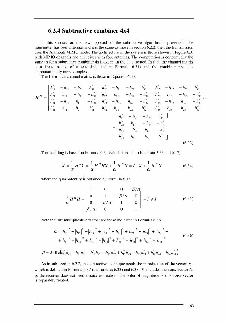
63
6.2.4 Subtractive combiner 4x4
In this sub-section the new approach of the subtractive algorithm is presented. The
transmitter has four antennas and it is the same as those in section 6.2.2, then the transmission
uses the Alamouti MIMO mode. The architecture of the system is those shown in Figure 6.3,
with MIMO channels and a receiver with four antennas. The computation is conceptually the
same as for a subtractive combiner 4x1, except in the data treated. In fact, the channel matrix
is a 16x4 instead of a 4x4 (indicated in Formula 6.31) and the combiner result is
computationally more complex.
The Hermitian channel matrix is those in Equation 6.33.
−−
−−
−−
−−
−−
−−
−−
−−
−−
−−
−−
−−
=
*
142434
*
44
*
241444
*
34
*
344414
*
24
*
443424
*
14
*
132333
*
43
*
231343
*
33
*
334313
*
23
*
433323
*
13
*
122232
*
42
*
221242
*
32
*
324212
*
22
*
423222
*
12
*
112131
*
41
*
211141
*
31
*
314111
*
21
*
413121
*
11
...
...
hhhh
hhhh
hhhh
hhhh
hhhh
hhhh
hhhh
hhhh
hhhh
hhhh
hhhh
hhhh
hhhh
hhhh
hhhh
hhhh
HH
(6.33)
The decoding is based on Formula 6.34 (which is equal to Equation 3.33 and 6.17).
NHXINHHXHYHXHHHH
αααα
1~111~+⋅=+== (6.34)
where the quasi-identity is obtained by Formula 6.35.
IIHH H ≠=
−
−=
~
100/
01/0
0/10
/001
1
αβ
αβ
αβ
αβ
α (6.35)
Note that the multiplicative factors are those indicated in Formula 6.36.
2
44
2
43
2
42
2
41
2
34
2
33
2
32
2
31
2
24
2
23
2
22
2
21
2
14
2
13
2
12
2
11
hhhhhhhh
hhhhhhhh
++++++++
++++++++=α (6.36)
( )*
342444
*
14
*
332343
*
13
*
322242
*
12
*
312141
*
11Re2 hhhhhhhhhhhhhhhh −+−+−+−⋅=β
As in sub-section 6.2.2, the subtractive technique needs the introduction of the vector X ,
which is defined in Formula 6.37 (the same as 6.23) and 6.38. X includes the noise vector N,
so the receiver does not need a noise estimation. The order of magnitude of this noise vector
is separately treated.

64
NH
xx
xx
xx
xx
x
x
x
x
xx
xx
xx
xx
H
α
αβ
αβ
αβ
αβ
αβ
αβ
αβ
αβ
1
/
/
/
/
~
~
~
~
/
/
/
/
14
23
32
41
4
3
2
1
14
23
32
41
+
⋅+
⋅−
⋅−
⋅+
=
=
⋅+
⋅−
⋅−
⋅+
(6.37)
=
×
−
−
−
−
−−
=
⋅+
⋅−
⋅−
⋅+
D
C
B
A
y
y
y
y
h
h
h
h
hhh
hhh
hhh
hhh
xx
xx
xx
xx
αα
αβ
αβ
αβ
αβ
1
......
...
...
...
1
/
/
/
/
44
*
31
*
21
11
*
14
*
24
*
34
*
44
2131
*
41
1141
*
31
4111
*
21
3121
*
11
14
23
32
41
(6.38)
The four lines of Formula 6.38 can be solved as indicated in Equation 6.25, so the
decoded values are written in Equation 6.39 (as in 6.26).
Λ−
Ψ=
Λ+
Ψ=
Λ+
Ψ=
Λ−
Ψ=
ADx
BCx
CBx
DAx
4
3
2
1
where
−=Ψ
2
2
1α
βα and
−=Λ
2
22
1α
β
β
α (6.39)
Note that in the case 4x4 antennas, the values of α and β are different.
The decoded noise vector can be calculated through Formula 6.40.
==
4
3
2
1
111
w
w
w
w
WNH H
ααα (6.40)
where W is the weighed noise vector. It is a vector of four elements, due to the matrix
product 4x16 by 16x1 of NHH
. These additional noise affects the received signals. These
components are called ei, where i indicates the receiving antenna, they are shown in Formula
6.41 (same of from 6.28 but with different α and β).
Λ−
Ψ−=→
Λ+
Ψ−=→
Λ+
Ψ−=→
Λ−
Ψ−=→
1444
2333
3222
4111
wwex
wwex
wwex
wwexvaluedecodedonnoise
(6.41)
It is difficult to quantitize the errors of the two techniques pseudo-inversion and
subtractive, but if considering that the two formulas are composed by the same variables, the
mathematical computation of the pseudo-inverse combiner needs more operations. This can
affect those system by more uncertainty.
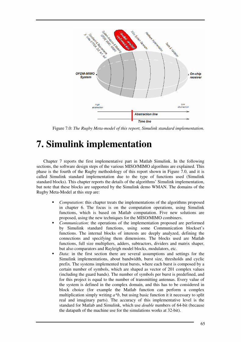
65
Figure 7.0: The Rugby Meta-model of this report, Simulink standard implementation.
7. Simulink implementation
Chapter 7 reports the first implementative part in Matlab Simulink. In the following
sections, the software design steps of the various MISO/MIMO algorihms are explained. This
phase is the fourth of the Rugby methodology of this report shown in Figure 7.0, and it is
called Simulink standard implementation due to the type of functions used (Simulink
standard blocks). This chapter reports the details of the algorithms’ Simulink implementation,
but note that these blocks are supported by the Simulink demo WMAN. The domains of the
Rugby Meta-Model at this step are:
� Computation: this chapter treats the implementations of the algorithms proposed
in chapter 6. The focus is on the computation operations, using Simulink
functions, which is based on Matlab computation. Five new solutions are
proposed, using the new techniques for the MISO/MIMO combiners.
� Communication: the operations of the implementation proposed are performed
by Simulink standard functions, using some Communication blockset’s
functions. The internal blocks of interests are deeply analyzed, defining the
connections and specifying them dimensions. The blocks used are Matlab
functions, full size multipliers, adders, subtractors, dividers and matrix shaper,
but also comparators and Rayleigh model blocks, modulators, etc.
� Data: in the first section there are several assumptions and settings for the
Simulink implementations, about bandwidth, burst size, thresholds and cyclic
prefix. The systems implemented treat bursts, where each burst is composed by a
certain number of symbols, which are shaped as vector of 201 complex values
(including the guard bands). The number of symbols per burst is predefined, and
for this project is equal to the number of transmitting antennas. Every value of
the system is defined in the complex domain, and this has to be considered in
block choice (for example the Matlab function can perform a complex
multiplication simply writing a*b, but using basic function it it necessary to split
real and imaginary parts). The accuracy of this implementative level is the
standard for Matlab and Simulink, which use double numbers of 64-bit (because
the datapath of the machine use for the simulations works at 32-bit).

66
� Time: the Simulink demo scheme transmits on a precise fixed bandwidth [24],
which is related to the bit-rate by an inverse relation. The Simulink systems are
working at a frequency related to the computer used for the simulations. Each
time instant is equivalent to a sample time (this relation can be modified by the
designer).
The abstraction line of Figure 7.0 indicates the implementation level, which has been
described in the four Rugby domains .
The WMAN Simulink demo is the basis for the blocks implemented in this project. The
subject of this chapter is the Simulink implementation of the new algorithms for the combiner
at the receiver.
Chapter 7 contains four sections sections, the first describes the reason of the WMAN
demo chioce and the settings for the whole system. The second section treats the case of
MIMO 2x2 antennas, with the replacement of the channel and the combiner block using the
classic Alamouti STBC mode. The cases of 4x1 and 4x4 are explained in section three, with
the implementation of the new approaches which have been proposed in chapter 6. The last
section propose a short discussion about the results and the motivation of why the MIMO 4x4
subtractive combiner has been chosen for the hardware implementation.
7.1. WMAN system and settings
As already indicated in the previous chapters, this project is based on an already existing
Simulink scheme, the WMAN IEEE 802.16d [24], [26]. The choise of this scheme is due to
the use of OFDM and MISO at the basis, moreover follows the IEEE 802.16d, one of the
most actuals [24] wireless comunication standard. The WMAN can be perfectly adapted to
this project, in order to develop, extend, simulate and test the new technique proposed. The
work done is the substitution of some blocks in order to develop an OFDM-MIMO with 2x2
antennas and OFDM-MISO/MIMO 4x1/4x4 system without any feedback. In the detail, the
work is:
� Extension of the MISO/MIMO transmitter for the various multiple antennas cases;
� Replacement of the pre-existent Rice channels with Rayleigh model channels;
� Substitution of the MISO 2x1 combiner (at the receiver), with the MIMO 2x2 and
the new MISO/MIMO decoders proposed in chapter 6;
� Extension of the OFDM transmitters/receivers for the various cases.
Figure 6.1 shows the architecture of the basic WMAN Simulink system, with an emphasis
on the blocks replaced. The blocks of interest are painted in blue and green: Space-Time
Diversity (STD) Encoder, OFDM Transmitters and Receivers, MISO/MIMO channels,
AWGN channels, Space-Time Diversity Combiner.
The Simulink Demo scheme provides some parameters for the setting of the
telecommunication system. Figure 7.1 shows the four configurations:
� Channel bandwidth, which indicates the total range of frequency of the channels,
in MHz. Note that this parameter is maintained constant for every case, at 3.5
MHz;
� Number of OFDM symbols per burst are set to 2 for the 2 transmitting antennas
systems and it is changed to 4 for the 4x1 and 4x4 schemes;
� Cyclic prefix factor indicates the entity of OFDM symbol part that is
retransmitted as guard band;
� Low SNR thresholds for rate control (dB) is a vector which indicates the 6
thresholds for the 7 modulations possible. In fact the system allows a change of
modulation (between BPSK ½, QPSK ½ or ¾, 16-QAM ½ or ¾, 64-QAM ²/3 or
¾ ) depending on the quality of the received signal.

67
Figure 7.1: The setting window of the WMAN scheme. The total channels bandwidth, the
number of OFDM symbols per burst, the cyclic prefix factor and the SNR thresholds for the
modulation are variable to specify.
In the next sections, the functional blocks implemented with standard Simulink devices
are explained. In the transmission chain the first of those blocks is the STD Encoder,
which has data bursts in input. By default, the structure of each data burst is a matrix with
201 rows (192 complex values for the 192 OFDM sub-carriers and 9 guard bands) and a
number of column equal to the symbols per burst.
7.2. MIMO 2x2
The first case is the introduction of a double antenna at the receiver. The transmitter is
working in Alamouti STBC mode and it was already implemented in the Simulink demo. So,
the development concerns the wireless channels and the 2x2 combiner.
7.2.1 The MIMO channels
The MIMO channels for this case are four and they are modeled as Rayleigh distribution.
Figure 7.2 shows the Simulink block of the channel and the AWGN. In Figure 7.3a) there is
the internal scheme of the channel block, with the four Rayleigh models. Figure 7.3b) shows
the AWGN internal block.
Figure 7.2: The scheme of the MIMO channels block and the AWGN for MIMO 2x2.

68
a) b)
Figure 7.3: a) The internal scheme of the MIMO channels b) the internal of the AWGN block.
The block MIMO channels in Figure 7.3a) represents not only the channels but also the
receiving antennas, because the adders and the gains are the model of them. Note that the
gain K are the same, and they represent the antenna attenuations. The AWGNs in Figure 7.3b)
are independents and affecting the signals on the receiving antennas. The scheme indicates
the input signals and the variance given by the Noise setting constant.
The settings for the Rayleigh channels are the same, resumed in Figure 7.4.
Figure 7.4: The setting window of the Rayleigh channel model with the parameters Maximum
Doppler shift, Delay vector, Gain vector and Initial seed..
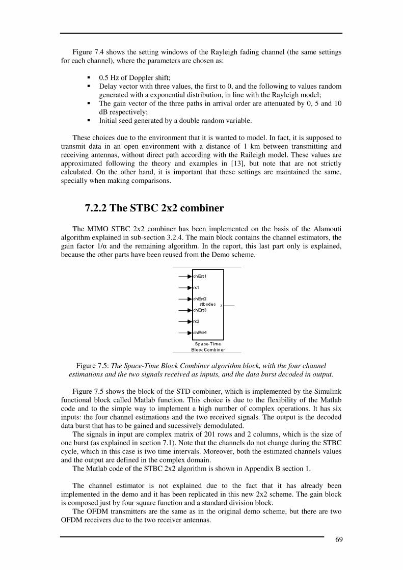
69
Figure 7.4 shows the setting windows of the Rayleigh fading channel (the same settings
for each channel), where the parameters are chosen as:
� 0.5 Hz of Doppler shift;
� Delay vector with three values, the first to 0, and the following to values random
generated with a exponential distribution, in line with the Rayleigh model;
� The gain vector of the three paths in arrival order are attenuated by 0, 5 and 10
dB respectively;
� Initial seed generated by a double random variable.
These choices due to the environment that it is wanted to model. In fact, it is supposed to
transmit data in an open environment with a distance of 1 km between transmitting and
receiving antennas, without direct path according with the Raileigh model. These values are
approximated following the theory and examples in [13], but note that are not strictly
calculated. On the other hand, it is important that these settings are maintained the same,
specially when making comparisons.
7.2.2 The STBC 2x2 combiner
The MIMO STBC 2x2 combiner has been implemented on the basis of the Alamouti
algorithm explained in sub-section 3.2.4. The main block contains the channel estimators, the
gain factor 1/α and the remaining algorithm. In the report, this last part only is explained,
because the other parts have been reused from the Demo scheme.
Figure 7.5: The Space-Time Block Combiner algorithm block, with the four channel
estimations and the two signals received as inputs, and the data burst decoded in output.
Figure 7.5 shows the block of the STD combiner, which is implemented by the Simulink
functional block called Matlab function. This choice is due to the flexibility of the Matlab
code and to the simple way to implement a high number of complex operations. It has six
inputs: the four channel estimations and the two received signals. The output is the decoded
data burst that has to be gained and sucessively demodulated.
The signals in input are complex matrix of 201 rows and 2 columns, which is the size of
one burst (as explained in section 7.1). Note that the channels do not change during the STBC
cycle, which in this case is two time intervals. Moreover, both the estimated channels values
and the output are defined in the complex domain.
The Matlab code of the STBC 2x2 algorithm is shown in Appendix B section 1.
The channel estimator is not explained due to the fact that it has already been
implemented in the demo and it has been replicated in this new 2x2 scheme. The gain block
is composed just by four square function and a standard division block.
The OFDM transmitters are the same as in the original demo scheme, but there are two
OFDM receivers due to the two receiver antennas.
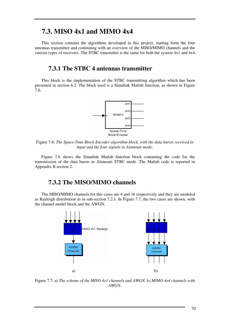
70
7.3. MISO 4x1 and MIMO 4x4
This section contains the algorithms developed in this project, starting form the four
antennas transmitter and continuing with an overview of the MISO/MIMO channels and the
various types of receivers. The STBC transmitter is the same for both the system 4x1 and 4x4.
7.3.1 The STBC 4 antennas transmitter
This block is the implementation of the STBC transmitting algorithm which has been
presented in section 6.2. The block used is a Simulink Matlab function, as shown in Figure
7.6.
Figure 7.6: The Space-Time Block Encoder algorithm block, with the data bursts received in
input and the four signals in Alamouti mode.
Figure 7.6 shows the Simulink Matlab function block containing the code for the
transmission of the data bursts in Alamouti STBC mode. The Matlab code is reported in
Appendix B section 2.
7.3.2 The MISO/MIMO channels
The MISO/MIMO channels for this cases are 4 and 16 respectively and they are modeled
as Rayleigh distribution as in sub-section 7.2.1. In Figure 7.7, the two cases are shown, with
the channel model block and the AWGN.
a) b)
Figure 7.7: a) The scheme of the MISO 4x1 channels and AWGN, b) MIMO 4x4 channels with
AWGN.

71
The blocks MISO/MIMO channels in Figure 7.7 are modeled exactly as the Rayleigh
channels of sub-section 7.2.1. Also the settings of the internal blocks remain the same, with
the same assumptions.
7.3.3 The MISO/MIMO STBC combiners
7.3.3.1 MISO 4x1 channel inversion combiner
The MISO 4x1 combiner with channel inversion is the implementation of the new
algorithm proposed in sub-section 6.2.1. It is based on the Alamouti transmission, but using a
channel inversion at the receiver. The algorithm for the combiner does not need the
multiplicative factor 1/α as the STBC 2x2. So, the main block contains two parts, the channel
estimation and the algorithm channel inversion. Figure 7.8 shows the implementation of the
algorithm channel inversion.
Figure 7.8: The 4x1 algorithm blocks. The first is the channel inversion and the second is the
combiner. The inputs are the four channel estimations, and the signal received. The output is
the decoded value.
Figure 7.8 shows the two blocks of the channel inversion combiner, excluding the
channel estimation. Both of them are implemented by Simulink Matlab functions. This choice
is due one more time to the flexibility of the text code and the high number of complex
operations. The inputs of the inversion block (on the left in Figure 7.8) are the estimated
values of the channels. The combiner (on the right in Figure 7.8) receive the channel
inversion and the signal from the antenna. The output is the decoded data burst.
Note that the signals are complex matrix of 201 rows and 4 columns, due to the size of
one burst set to 4 symbols. The channels do not change during the STBC cycle, which in this
case is four time intervals.
The Matlab code of the channel inversion and the 4x1 combiner is shown in Appendix B
section 3.
The channel estimator has been replicated in order to estimate the four MISO channels.
Note that the algorithm has not additional gain blocks.
The OFDM transmitter has been reused and replicated four time, adapting the preambles
for the transmission.
7.3.3.2 MISO 4x1 channel pseudo-inversion combiner
This combiner with channel pseudo-inversion is a reduction of the case 4x4 to the 4x1.
The implementation is done in order to have a comparison between channel inversion and
pseudo-inversion. As in the case explained in sub-section 7.3.3.1, there is not the

72
multiplicative factor 1/α. The main block contains two parts, the channel estimation, which is
the same as in the previous case, and the second part is the pseudo-inversion combiner. In
Figure 7.9 the implementation of this algorithm is shown.
Figure 7.9: The 4x1 algorithm blocks for the pseudo-inversion. The first is the pseudo-
inversion of the channel and the second is the combiner. The inputs are the four channel
estimations, and the signal received. The output is the decoded value.
In Figure 7.9 the second part of the main block, without channel estimation is shown. The
two blocks are implemented by Simulink Matlab functions and the code of the pseudo-
inverter is reported in Appendix B section 4. Note that the pseudo-inversion combiner, the
signals and the inputs are exactly the same as for the case of channel inversion. The other
settings are equals to those indicated in sub-section 7.3.3.1.
7.3.3.3 MISO 4x1 subtractive combiner
The last case of 4x1 combiner is those that perform the new subtractive algorithm of sub-
section 6.2.2. Transmission and reception are based on the Alamouti STBC mode. The only
difference is a subtractive technique with the purpose to reduce the interference which the
non-identity introduces.
The scheme is proposed in Figure 7.10, and it contains two blocks, the subtractive
combiner and the gain compensator & interference corr. The first calculates the product YHH
defined in Formula 6.17, while the second perform the interference correction.
Figure 7.10: The 4x1 algorithm blocks for the pseudo-inversion. The first is the pseudo-
inversion of the channel and the second is the combiner. The inputs are the four channel
estimations, and the signal received. The output is the decoded value.

73
The combiner block, on the left of Figure 7.10, is implemented by a Matlab function,
while the gain compensator and interference corr., on the right of Figure 7.10 contains
Simulink operators as multipliers, dividers and additions. Both the two blocks receive the
channels estimations as inputs. The first processes also the received signal, while the second
receive the decoded burst with interference, where z is the normal shaped burst (201x4) and
zinv the same burst with inverted order of column (to make simpler the interference
subtraction). The output is the decoded data burst.
The matlab function performed by the left block of Figure 7.10 is shown in Appendix B
section 5. The internal operators of the right block are shown in Figure 7.11.
Figure 7.11: The gain compensator & interference corr. block. The two burst (in input 3 and
6) are divided by the gains according with Formula 6.26. The output is the decoded value.
Figure 7.11 shows the internal Simulink operators of the gain compensator & interference
correction block. This scheme calculates the values of Ψ and Λ (as indicated on the wires in
Figure 7.11), according with Firmula 6.26, and it divides the burst signals by them.
7.3.3.4 MIMO 4x4 channel pseudo-inversion combiner
The MIMO 4x4 combiner with the channel pseudo-inversion process the new technique
proposed in sub-section 6.2.3. It decodes the signals transmitted in Alamouti STBC mode, but
at the receiver it uses the pseudo-inversion to compute the data. The main block contains two
parts, the channel estimation and the algorithm channel pseudo-inversion. Figure 7.12 shows
the implementation of the algorithm channel pseudo-inversion.
Figure 7.12 shows the two blocks of the channel pseudo-inversion algorithm, excluding
the channel estimation, which has been replicated for the 16 MIMO channels. Both are
implemented by Simulink Matlab functions. The inputs of the pseudo-inversion block, on the
left in Figure 7.12, are the estimated values of the 16 channels. The combiner, as for the case
with 4x1 antennas, receive the channel pseudo-inversion and the signals from the various
antennas. The output represents the decoded data burst.
The Matlab code of the channel inversion and the 4x1 combiner is shown in Appendix B
section 6.
Note that the channel estimator has been replicated to estimate the 16 MIMO channels,
and the OFDM receiver has been reused four time to perform the 4x4 transmission.

74
Figure 7.12: The 4x4 algorithm blocks. The first is the channel pseudo-inversion and the
second is the combiner.
7.3.3.5 MIMO 4x4 subtractive combiner
The last combiner proposed is the new subtractive algorithm for 4x4 receiver introduced
in sub-section 6.2.4. The Alamouti STBC mode is at the basis of the transmission and the
reception. An additional part has the purpose to subtract the interference as the technique
proposed in sub-section 6.2.4. In Figure 7.13 the subtractive combiner is shown.
Figure 7.13: The 4x4 scheme of the subtractive technique. The central block is the combiner
for the product YHH , the five blocks around perform addition of the squared for the gain
calculation. The right block calculate the decoded signal reducing the interference effect.

75
The scheme in Figure 7.13 is composed by the subtractive combiner and 5 blocks which
calculate the first part of the gain parameters. The last block is the gain compensator and
interference correction. The subtractive combiner calculates the product YHH defined in
Formula 6.34 and the others perform the new subtractive approach. The subtractive combiner
has several inputs: the 16 channel estimations and the 4 signals received by the antennas. The
output is the decoded burst. The central block of Figure 7.13 is implemented by a Matlab
function, which code is the those indicated in Appendix B section 7, similar to for the
pseudo-inversion case, but with different signs and a final additional line at the end of the for
loop: zinv(:, [4*i-3 4*i-2 4*i-1 4*i]) = [-z3 z2 z1 -z0];
The other blocks of Figure 7.13 are implemented by Simulink standard operators, as for
the case of sub-section 7.3.3.3. These operators perform the values of of Ψ and Λ calculated
in Formula 6.36 and 6.39.
7.4. Simulation discussion
In this section a discussion on the comparison between the five MISO/MIMO systems of
section 7.3 is proposed. This because it wants to explore the quality of the various new
techniqes respect to the Simulink demo scheme. Moreover, the second objective of this
project is to implement in hardware a part of a MISO or MIMO combiner. Once chosen the
algorithm to design, the focus is on just a part of the combiner, due to the hardware design
approach for this project. In fact it consists in start implementing just a part of the system,
that certainly can fit the FPGA. This choice is qualitative and is related to the designer
background, considering the cost function (defined in chapter 5).
The quality exploration of the five systems is done by several Simulink simulations and
analyzing the results in terms of Bit error rate varying the SNR. Note that every other design
parameters must be constant. The description of the simulation environment, the settings and
the results are explained in the chapter 10. The choice of the algorithm to implement in
hardware is due to two analysis:
� Qualitative: comparing the five system implemented in Simulink, the first input
for the designer is the number of antennas used. Probabily the 4x4 antennas
systems have a better transmission quality (in terms of throughput) than the 4x1s.
By this thesis the comparison can be done on the two decoding noises introduced
by the two 4x4 techniques (Formulas 6.32 and 6.41). The discussion at the end of
section 6.2.4 reports that the noise of the MIMO 4x4 with subtractive combiner is
lower, that means a better Bit Error Rate (BER) and then throughput.
Note that the sentence regarding the number of antennas is a simple deduction,
however the practical simulations can show completely different results, so this
justifies a quantitative analysis.
� Quantitative: the various MISO/MIMO systems has been simulated maintaining
the same configuration parameters and varying the SNR on the transmission. The
metric BER has measured by 100 simulation for each case of SNR. Finally the
trends has been shown on a graph in chapter 10.
Looking at these results, the BER curve of the 4x4 with subtractive technique
appears the lower respect to the other 4 solutions. In fact the BER is inversely
proportional to the throughput, assuming the same modulation. Assuming the
initial constraints of fixed bandwidth and transmission power, the conclusion is
that the smaller SNR needed to transmit at the same bit rate is those of the 4x4
subtractive system.
Once identified the algorithm to implement, the next step is to chose the part which must
be designed on the target FPGA. The approach used in the next chapters is to start with just a
part of the receiver, and in particular of the new subtractive technique. This due to the limited
computational resources available on the FPGA and, in general, the cost function (chapter 5).
This last objective involves a trade-off between execution time and area. In chapter 8 follows
a discussion about.

76
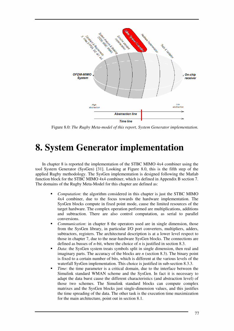
77
Figure 8.0: The Rugby Meta-model of this report, System Generator implementation.
8. System Generator implementation
In chapter 8 is reported the implementation of the STBC MIMO 4x4 combiner using the
tool System Generator (SysGen) [31]. Looking at Figure 8.0, this is the fifth step of the
applied Rugby methodology. The SysGen implementation is designed following the Matlab
function block for the STBC MIMO 4x4 combiner, which is defined in Appendix B section 7.
The domains of the Rugby Meta-Model for this chapter are defined as:
� Computation: the algorithm considered in this chapter is just the STBC MIMO
4x4 combiner, due to the focus towards the hardware implementation. The
SysGen blocks compute in fixed point mode, cause the limited resources of the
target hardware. The complex operation performed are multiplications, additions
and subtraction. There are also control computation, as serial to parallel
conversions.
� Communication: in chapter 8 the operators used are in single dimension, those
from the SysGen library, in particular I/O port converters, multipliers, adders,
subtractors, registers. The architectural description is at a lower level respect to
those in chapter 7, due to the near-hardware SysGen blocks. The connections are
defined as busses of n-bit, where the choice of n is justified in section 8.3.
� Data: the SysGen system treats symbols split in single dimension, then real and
imaginary parts. The accuracy of the blocks are n (section 8.3). The binary point
is fixed to a certain number of bits, which is different at the various levels of the
waterfall SysGen implementation. This choice is justified in sub-section 8.3.3.
� Time: the time parameter is a critical domain, due to the interface between the
Simulink standard WMAN scheme and the SysGen. In fact it is necessary to
adapt the data burst cause the different characteristics (and abstraction level) of
those two schemes. The Simulink standard blocks can compute complex
matrixes and the SysGen blocks just single-dimension values, and this justifies
the time spreading of the data. The other task is the execution time maximization
for the main architecture, point out in section 8.1.

78
The bottom part of Figure 8.0 indicates the progress step on the abstraction line, close to
the final hardware implementation, according with the accurate description of the 4 Rugby
domains.
Chapter 8 treats four sections, Motivation with a justification of several design choice,
follows an overview on the System Generator blocks used. The third section detail the
SysGen implementation proposed in this report. The chapter is closed with a short discussion
on the resource estimation, which is accurately reported in the Result chapter.
8.1. Motivations
The tool for the implementation of this part is Xilinx System Generator [31]. The choice
is due to the simple interface between software and hardware that that tool provides [32], [33].
In fact by System Generator it is possible to create a scheme in Simulink using Xilinx
libraries. The advantage of the these blocks provided by Xilinx is that the Simulink scheme
can be synthesized directly into a bit stream file for the FPGA. Moreover, using input and
output ports it is possible connecting Simulink standard blocks with those of SysGen.
Considering that the project described in this report is a possible implementation for
telecommunication system, the first objective of the designer is to minimize the execution
time, in order to have the faster bit-rate as possible. The second thing, but not less important,
is to minimize the area in terma of resourses usage. However, note that the maximum rate is
the main objective that the designer want to obtain, within reason. So, for this particular task,
the execution time has been prioritized, while for the others design trade-offs the two metrics
(execution time and area) have the same priority.
As already indicated, the main objective is achieving the maximum bit-rate possible for
the chosen scheme. To do that it is necessary to introduce an additional constraint: chose the
maximum level of parallelism as possible, that is equivalent to exclude the area metric from
the cost function (section 5.1). Note that this exception is just for this task. The draw-back of
this choice is an high number of resources.
The designing consequence of this choice is that the area metric must be optimized in
other way. One of that can be use a bit-accuracy as low as possible, but preserving the quality
of the system. This matter introduce another trade-off: area vs. accuracy-errors (discussed in
this chapter). Anyway there is another way to optimize the area usage, the use of operators at
the lowest abstraction level as possible, avoiding the multifunctional or composed operators
(not optimized).
As indicated in section 7.4, the hardware implementation concerns just a part of the
receiver, and more precisely a part of the MIMO 4x4 subtractive combiner. This due to the
design approach that has been explained in section 7.4, which consists in chosing a relative
small part to implement in hardware. Relative small means that this part must fit the size of
the FPGA, knowing the number of available resources. The main features of the target FPGA
Virtex 5 xc5vls50t are [28]:
� Number of slice registers: 32,640 (number of full slices 8,160);
� Nr. of conigurable I/O ports: 480 bit;
� Nr. of DSP48E devices (25x18 multiplier, adder and accumulator): 288;
� Max block RAMs: 4,752 Kb.
The first idea was to implement a part of the MIMO 4x4 subtractive combiner, those
which perform the Matlab function indicated in Appendix B section 7 (called function “dec”).
Looking at the operations, the first think to consider is the using of complex values. This is
fundamental to estimate the area of the SysGen implementation (i.e. a complex multiplication
needs four real domain (simple) multipliers, an adder and a subtractor). Applying this
approach to the algorithm considered, the designer estimation is:
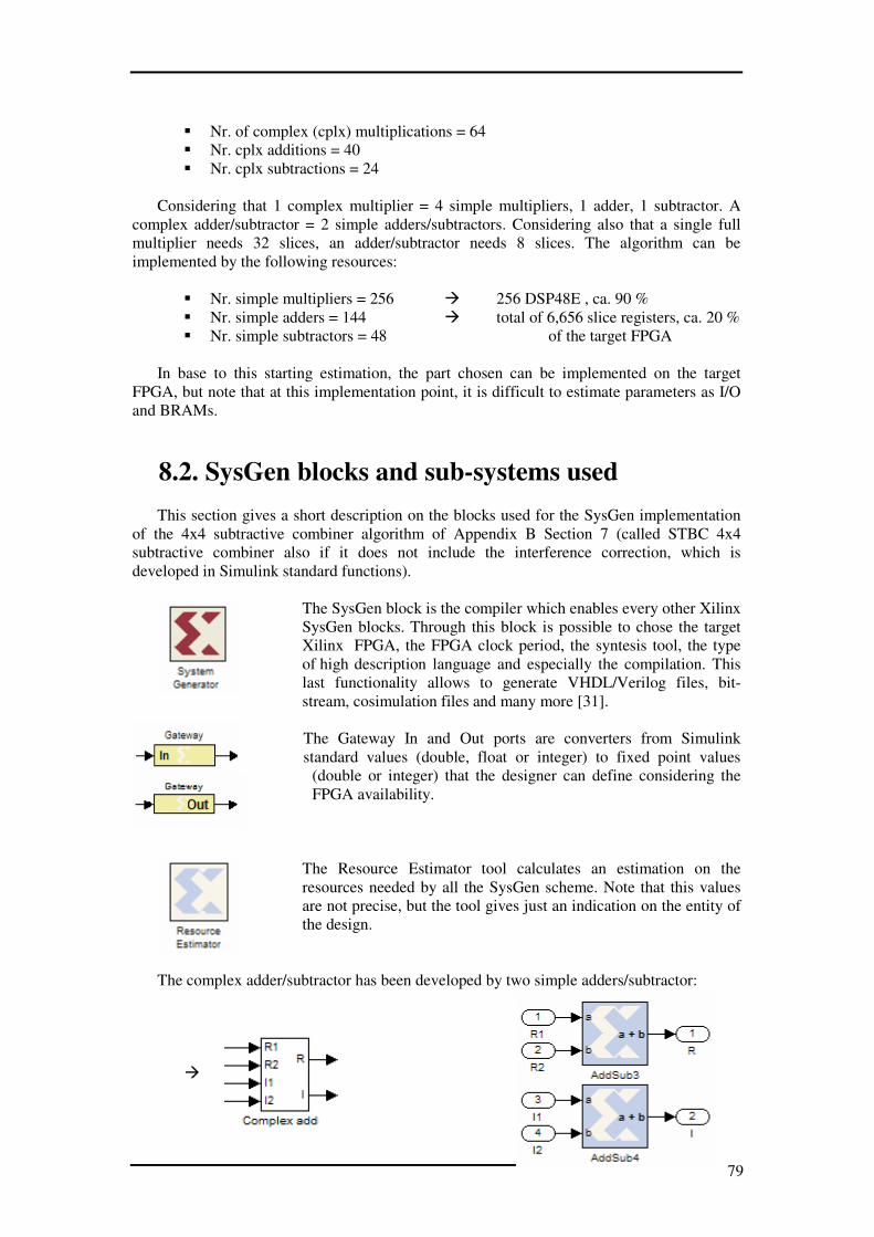
79
� Nr. of complex (cplx) multiplications = 64
� Nr. cplx additions = 40
� Nr. cplx subtractions = 24
Considering that 1 complex multiplier = 4 simple multipliers, 1 adder, 1 subtractor. A
complex adder/subtractor = 2 simple adders/subtractors. Considering also that a single full
multiplier needs 32 slices, an adder/subtractor needs 8 slices. The algorithm can be
implemented by the following resources:
� Nr. simple multipliers = 256 � 256 DSP48E , ca. 90 %
� Nr. simple adders = 144 � total of 6,656 slice registers, ca. 20 %
� Nr. simple subtractors = 48 of the target FPGA
In base to this starting estimation, the part chosen can be implemented on the target
FPGA, but note that at this implementation point, it is difficult to estimate parameters as I/O
and BRAMs.
8.2. SysGen blocks and sub-systems used
This section gives a short description on the blocks used for the SysGen implementation
of the 4x4 subtractive combiner algorithm of Appendix B Section 7 (called STBC 4x4
subtractive combiner also if it does not include the interference correction, which is
developed in Simulink standard functions).
The SysGen block is the compiler which enables every other Xilinx
SysGen blocks. Through this block is possible to chose the target
Xilinx FPGA, the FPGA clock period, the syntesis tool, the type
of high description language and especially the compilation. This
last functionality allows to generate VHDL/Verilog files, bit-
stream, cosimulation files and many more [31].
The Gateway In and Out ports are converters from Simulink
standard values (double, float or integer) to fixed point values
(double or integer) that the designer can define considering the
FPGA availability.
The Resource Estimator tool calculates an estimation on the
resources needed by all the SysGen scheme. Note that this values
are not precise, but the tool gives just an indication on the entity of
the design.
The complex adder/subtractor has been developed by two simple adders/subtractor:
�

80
�
The complex multiplier has been implemented by specific gains (motivated in the next
sections), four multipliers, an adder and a subtractor, four registers. The conjugation function
has been involved to optimize the area metric:
�

81
8.3. SysGen STBC 4x4 subtractive combiner
This section contains the entire SysGen implementation of the STBC 4x4 subtractive
combiner with the external blocks and the connections.
The system developed is composed by:
� Inputs/Outputs
� Multiplier bank
� Adders/subtractors banks
Figure 8.1 shows the scheme implemented and emphasis on the main blocks.
Figure 8.1: The STBC 4x4 subtractive combiner scheme which has been implemented in
SysGen blocks. The INputs & OUTputs are on the left and right respectively, the
MULTipliers on the the center-left and the ADDers SUBtractors on the center-right.
Note that the main WMAN-MIMO 4x4 scheme with subtractive technique has been split
from the SysGen implementation into two different files. This due to the different working
frequency. The SysGen application works 201 times faster than the WMAN scheme (201
cause the OFDM symbol structure, see section 7.1). This create problems during the
simulations, cause the computer used has not enough resources to process the entire scheme.
Moreover the WMAN scheme compute a burst for each time instant (complex matrix 201x4

82
one Simulink sample), while the SysGen implementation uses single dimension values with a
limited number of bits. In other words, one burst has to be spread into 201 SysGen samples.
To perform this step has been developed a specific Matlab code in order to interface the two
schemes. The idea is to lunch a simulation of the WMAN scheme and save the data in input
of the STBC combiner (after the channel estimation) using specific Simulink standard blocks.
Once saved the data, the Matlab interface functions spreads the bursts into single dimension
data readable by the SysGen scheme. The next step is to simulate the SysGen scheme file and
save these results, which are re-shaped for the WMAN scheme by the secon Matlab interface
function. Re-opening the WMAN scheme and lanching the simulation with the saved file it is
possible to analyze the final results. It is also possible to make comparison between the
results of the two implementation, those by Simulink standard and those by System Generator
blocks. All these configurations, interfaces, results and comparisons are explained in the
results chapter.
Note that the design choice for the datapath on the FPGA is 8-bit. This is due to the
following reasons:
� Minimization of the cost function concerning the area metric
� Fit the datapath to the commercial sizes (8, 10, 12-bit) starting with the less bits-
solution
� 8-bit is the minimum accuracy to keep the system working
� Reduce the datapath as possible for energy consumption.
8.3.1 Inputs and outputs
The input block on the left of Figure 8.1 contains the interface Simulink standard-to-
SysGen. These data are the 4 received signals and the 16 channels estimations. Inside the
main block there are Simulink standard blocks “From Workspace” that provide the inputs
from the WMAN scheme (opportunely pre-saved by blocks “To Workspace”). Each signal
has been saved in single dimension, so the complex parts have been split in order to provide
data that the SysGyen blocks can process.
Figure 8.2 shows one of the 4 banks of From Workspace blocks connected to the
Gateway Ins.
Figure 8.2: One of the 4 banks of inputs corresponding to the signal received at the first
antenna in the 4 instants. The real parts is split from the imaginary. From Workspace blocks
provides the input vectors, which are conseguently divided into single values.

83
Figure 8.2 shows one of the received signal at antenna 1 in the 4 various time instants.
The complex values has been already split into real-imaginary parts in the WMAN scheme
before the blocks To Workspace. From Workspaces blocks provides the input vectors of 4
columns, which are conseguently divided into single values. In fact, the Gateway Ins accept
only single-dimension values.
Figure 8.3 shows one of the banks of conversion for the channel estimation values.
Figure 8.3: One of the 4 banks of inputs corresponding to 4 channels estimations. The real
parts is split from the imaginary. Note that, as assumed, the channel does not change during
the four time intervals of the STBC cycle. The signals coming from the Workspace has been
bufferized to have vectors of 4 elements to the Gateway Ins. Sucessively the signal are
parallelized.
Figure 8.3 shows one of the 4 banks of inputs From Workspace which are the information
about 4 channels estimations. The complex values has been pre-split. As assumed for the
STBC mode, the channel does not change during the four time intervals. Moreover, the
channels estimations has been bufferized in the WMAN scheme, to have vectors of 4
columns. After the SysGen Input ports, the signal are parallelized by the Out_pipe blocks.
The choice to bufferize the channels estimations is forced cause the limited number of
inputs of the target FPGA:
� Total nr. of configurable I/O ports of Virtex 5 xc5vsx50t = 480 bits
Estimation of the SysGen I/O considering that they are converting 64-bit (double) to 8-bit
fixed point.:
� Nr. of Output needed = 4 ports of 8-bit � 32 bits
� Nr. of Input needed by received signals = 32 ports of 8-bit � 256 bits
� Nr. of Input needed by channel estimation = 32 ports of 8-bit � 256 bits
544 bits
Maintaining the channels estimations in standard notation (as the received signals) the
implementation would not be possible. This justifies the proposed solution of the bufferized
channels estimations, that is possible cause the values do not change before 4 time intervals.
Figure 8.4 points out this design choice.

84
Figure 8.4: The bufferization of the channels estimations. Note that the four channels
indicated as example, the data have already split, so this can be the 4 real parts of the 16
channels. The SysGen sample lines shows 4 time instants.
That implementation does not need changing in the SysGen-sample time of the SysGen
scheme, but not that it introduces a delay of 4 samples.
The final estimation of the total number of I/O is:
� Nr. of Output needed = 4 ports of 8-bit � 32 bits
� Nr. of Input needed by received signals = 32 ports of 8-bit � 256 bits
� Nr. of Input needed by channel estimation = 8 ports of 8-bit � 64 bits
352 bits
This approach allows the implementation on the target FPGA, with just a draw-back
about the 4 SysGen samples of delay.
The output of the Gateway In blocks are then the inputs of the SysGen system
implemented.
8.3.2 Multipliers bank
The four emphsized blocks on the center-left of Figure 8.1 are the Multipliers bank.
These operations perform the maximum possible parallelism for this SysGen implementation.
In fact the complex multipliers are developed in parallel, using the complex multiplier block
defined in secion 8.2. The total number of complex multiplication is 64, that is equal to 256
simple multipliers.
The settings windows of the SysGen complex multiplier blocks are defined as:
� Gain multiplication:
o Constant value set to 0.0078125 to obtain a reduction of the inputs
smaller than the value 1. (This choice is due to the simpler bit settings on
the following blocks). Number of bits for the gain = 8 with 8-bit binary
point;
o Latency = 0;
o Output type precision with Signed (2’s complement) Output type, 8-bit
with 7-bit of binary point, Rounding quantization and Saturating
overflow.
o Distributed RAM Memory type.
� Simple Multipliers:
o User defined precision with Signed (2’s complement) Output type, 8-bit
with 7-bit of binary point, Rounding quantization and Saturating
overflow;
o Latency = 3 SysGen samples (minimum to allow the pipelining);
Channel 11 … 27.43 …
Bufferized channels estimations
Channel 21 … 21.33 …
… 27.43 21.33 4.02 127.78 …
Channel 31 … 4.02 …
Channel 41 … 127.78 …
SysGen samples SysGen samples
… 11 12 13 14 15 … … 11 12 13 14 15 …

85
o Implementation using embedded multipliers DSP48E [28] core parame-
ters, optimized for speed and testing for optimum pipelining.
� Registers:
o Standard settings. Delay =1.
� Simple Adders/Subtractors:
o Latency = 0.
o User defined precision with Signed (2’s complement) Output type, 8-bit
with 7-bit of binary point, Rounding quantization and Saturating
overflow;
o Implementation using behavioral HDL.
8.3.3 Adders/Subtractors banks
The emphsized blocks on the center-right of Figure 8.1 are the four banks of Additions
and Subtractions (concerning just the 3 blocks on the top of the last bank). These operations
perform the algorithm using as less resources as possible, in a waterfall architecture. The
scheme uses the complex additions/subtractions blocks defined in secion 8.2.
The settings windows of the SysGen complex adders/subtractors blocks are defined as:
� Simple Adders/Subtractors:
o Latency = 0.
o User defined precision with Signed (2’s complement) Output type, 8-bit
with a scaled nr. of bits of binary point, Rounding quantization and
Saturating overflow. The scaled number of binary points means 6-bit for
the first 2 banks, 5-bits for the third bank and the fourth bank 4-bit. This
is due to the output values, where this configuration is a trade-off
between accuracy and saturation (in total 8-bit available).
o Implementation using behavioral HDL.
Note that every setting for each SysGen block has been chosen after many simulations
and corrections, folowing the approach proposed in section 2.5 concerning the cyclic design
flow. Those indicated are the final configurations.
Note that the registers before the simple subtractors have been introduced due to
hardware implementations. In fact, the subtractors need more time than the adders to perform
the operations. However this problem is pointed out in the Result section.
8.4. SysGen Resource Estimator
The tool Resource estimator defined in section 8.2 gives an indication on the resources
needed by the scheme on FPGA. Note that this tool does not provide a precise estimation,
cause it does not consider the model of target FPGA, but just a number of pre-defined number
of resources [31].
Anyway, Resource Estimator gives useful information also during the SysGen
development, in order to have an indication on the area/resources which are needed for the
target scheme.
In Results section is reported the final resource estimation obtained lanching this tool.
Looking at this results, every number respect the limit given by the target Virtex 5 FPGA
xc5vsx50t.

86

87
Figure 9.0: The Rugby Meta-model of this report, Hardware implementation.
9. Hardware implementation
Chapter 9 reports the hardware implementation of the STBC MIMO 4x4 combiner
designed in this project. The Virtex 5 xc5vsx50t FPGA is the target which supports the
system developed. The bit-stream is generated using the tool System Generator [31]. In
particular, the bit stream file is sythesized for SW/HW co-simulation.
Figure 9.0 shows the implementation step on the applied Rugby methodology, where the
four domains are defined as:
� Computation: the algorithm considered in this chapter is the same as those of
chapter 8, but implemented on hardware. This means that the calculation of the
STBC MIMO 4x4 combiner is performed by the FPGA, which allows a parallel
computation instead of a serial-pipelined one (operation by operation, even if
optimized by pipeline), as those performed by the computer hardware. At this
abstraction level, the HW operations (multiplications, additions, subtractions and
data conversions) can be defined by differential equations between physical
signals.
� Communication: the HW operators are working in single dimension as constraint
of the target FPGA. In particular they are I/O port converters, multipliers, adders,
subtractors, registers. Note that this operators are implemented by apposite
resources, as the DSP48E [28] in the case of the multipliers, and by standard
slice blocks for every others operators. The placement is automatically
implemented by the SysGen compiler. This compiler performs also the routing,
just in the next synthesis step, providing the physical connections between slices.
Note that this very low abstraction level (gates and wires) has not been detailed
cause reported in the files provided by the sysnthesis netlist (in the CD-ROM
attached to this report).
� Data: the FPGA works in 8-bit fixed point binary format. In this chapter, the
abstraction level defines the data as physical signals defined by voltage and
currents.

88
� Time: the time parameters are characterized by the physical behavior of the
signals inside the FPGA. The gates composing the slices introduce delays which
can not be neglected. About this aspect there is a discussion in Chapter 10
concerning the length of the longest path of the hardware implemented.
The bottom part of Figure 9.0 indicates the low abstraction level of this hardware
implementation.
Chapter 9 is divided in two sections, at first a short description on the board which
supports the target FPGA, the second shows the hardware implementation with an overview
of the SW/HW co-simulation which supports the testing of this project.
9.1. ML506 board
The target FPGA is Xilinx Virtex 5 xc5vsx50t, which is fitted put on the platform ML506.
This board has been provided by the Aalborg University’s CSDR. The ML506 platform is
one of the last products from Xilinx, and has the following main features [29]:
� Xilinx Virtex 5 FPGA xc5vsx50t-1ffg1136;
� Two PROMs of 32 MB;
� CompactFlash interface;
� 8 DIP switches, 8 leds, pushbottons and rotary encoder, 16-character x 2-line
LCD display;
� RS-232, DVI, JTAG, Ethernet and USB ports.
The features indicated are just a few for obvious reasons, the others are reported on [29].
The FPGA Virtex 5 xc5vsx50t is one of the smallest chip of that series [28], and the main
characteristics can be resumed as follows:
� 8160 slices;
� 780 KB of distributed RAM;
� 288 DSP48E advanced embedded multiplier;
� 4752 KB of Block RAM blocks;
� 15 I/O banks with a total of 480-bit configurable ports.
Note that also in this case for reporting reasons, just the main features fundamental for
this report has been indicated, but the detailed characteristics are explained in [28]. Moreover
in Appendix E Figure 9.1, an image of the board ML506 is shown.
9.2. SW/HW co-simulation
9.2.1 Introduction
As indicated in sub-section 5.3.1, thanks to the tools provided by Matlab-Simulink [30],
Xilinx ISE and System Generator for DSP [31], is possible to build a complete hardware-
testing environment called HW/SW co-simulation [32]. It consists in a real-time Simulink
simulation with hardware-in-the-loop, where the software algoithms are running at the same
time of the FPGA. In this way the communication allows the exchange of data and the
comparison of the results, but it is also possible to compute the signals from the hardware in
following Simulink standard blocks. Of course there are special interfaces and settings to do,
details which are explained in the hardware implementation chapter. However for this project
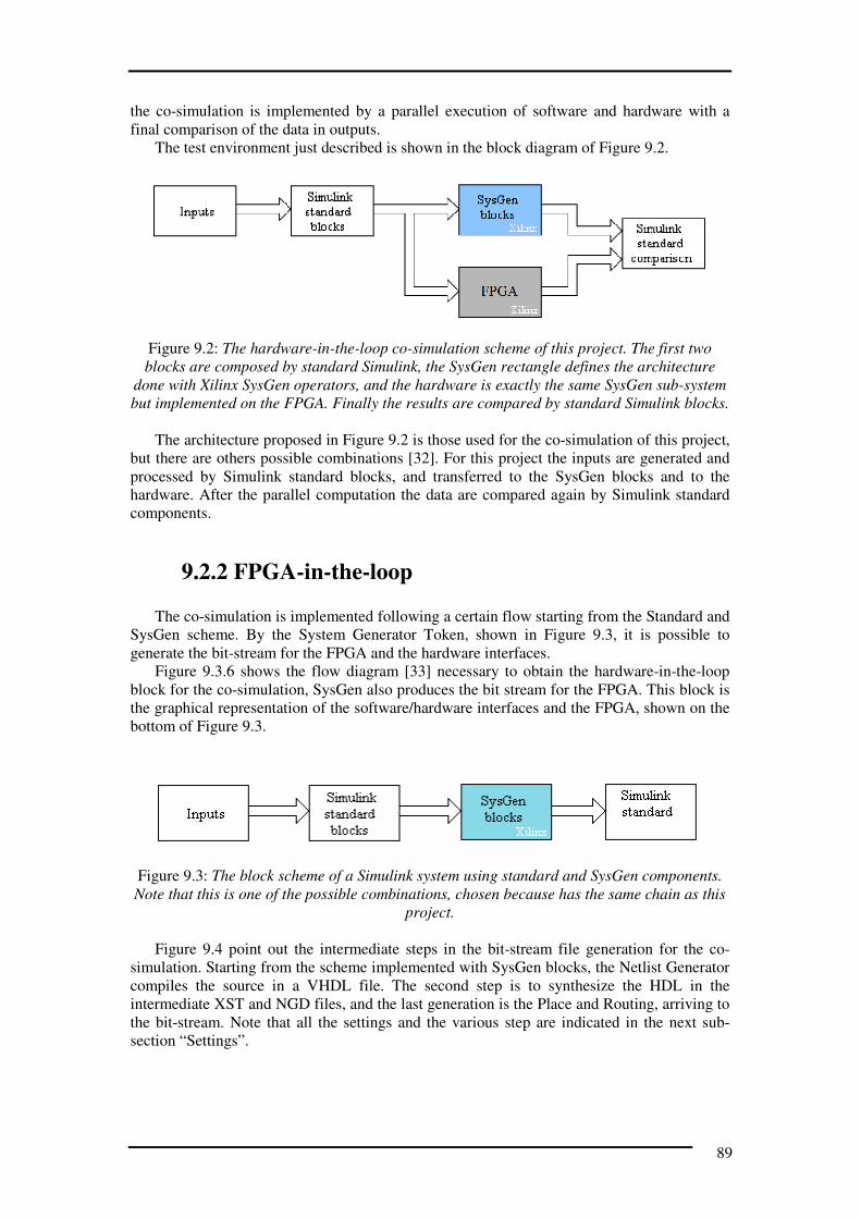
89
the co-simulation is implemented by a parallel execution of software and hardware with a
final comparison of the data in outputs.
The test environment just described is shown in the block diagram of Figure 9.2.
Figure 9.2: The hardware-in-the-loop co-simulation scheme of this project. The first two
blocks are composed by standard Simulink, the SysGen rectangle defines the architecture
done with Xilinx SysGen operators, and the hardware is exactly the same SysGen sub-system
but implemented on the FPGA. Finally the results are compared by standard Simulink blocks.
The architecture proposed in Figure 9.2 is those used for the co-simulation of this project,
but there are others possible combinations [32]. For this project the inputs are generated and
processed by Simulink standard blocks, and transferred to the SysGen blocks and to the
hardware. After the parallel computation the data are compared again by Simulink standard
components.
9.2.2 FPGA-in-the-loop
The co-simulation is implemented following a certain flow starting from the Standard and
SysGen scheme. By the System Generator Token, shown in Figure 9.3, it is possible to
generate the bit-stream for the FPGA and the hardware interfaces.
Figure 9.3.6 shows the flow diagram [33] necessary to obtain the hardware-in-the-loop
block for the co-simulation, SysGen also produces the bit stream for the FPGA. This block is
the graphical representation of the software/hardware interfaces and the FPGA, shown on the
bottom of Figure 9.3.
Figure 9.3: The block scheme of a Simulink system using standard and SysGen components.
Note that this is one of the possible combinations, chosen because has the same chain as this
project.
Figure 9.4 point out the intermediate steps in the bit-stream file generation for the co-
simulation. Starting from the scheme implemented with SysGen blocks, the Netlist Generator
compiles the source in a VHDL file. The second step is to synthesize the HDL in the
intermediate XST and NGD files, and the last generation is the Place and Routing, arriving to
the bit-stream. Note that all the settings and the various step are indicated in the next sub-
section “Settings”.

90
Figure 9.4: The flow diagram of the co-simulation generation by SysGen. The input files
is the sub-scheme with SysGen blocks, the first step is the Netlist generation, after the
Synthesis of the HDL file and finally the Xflow generation.(Inspired by SysGen tool).
The grey block on the bottom of Figure 9.4 represents the bit stream file generate for the
target FPGA. In the next sub-section the settings to execute the bit-stream generation is
shown.
9.2.3 Settings for hardware implementation
Figure 9.5: The SysGen generation window configuration. The co-simulation is chosen,
with the target board and the transmission cable, the FPGA, the tool used for the synthesis
and the HDL type. There are also options for the clocking.

91
Note that the versions of the various tools for the co-simulation implementation are:
� Matlab version 7.6.0.324 (R2008a), from [30];
� Simulink 7.1.1. (R2008a+) from [30];
� Xilinx ISE Design Suite 11.1 (including System Generator for DSP 11.1).
Documentation in [31], [32];
Figure 9.5 shows the various settings for the co-simulation block generation:
� Compilation
o ML506 selected board, with a point to point transmission through
Ethernet standard. This chioce is due to the fact that the connection
computer-platform is direct without any external network support (i.e.
Internet). Ethernet is the only connection type provided by this version of
System Generator;
o Virtex 5 FPGA xc5vsx50t -1ff1136, which indicates the FPGA type
(xc5vsx50t), the speed grade (-1) and the case type (ff1136);
o Synthesis tool the standard XST;
o Language VHDL (VHSIC (Very High Speed Integrated Circuits) High
Description Language).
� Clocking options
o FPGA clock period 10 ns, which is the minimum value between 10, 15,
20 and 30 ns;
� Simulink system period set to 1, as for default.
The co-simulation file has been generated by SysGen as shown in Figure 9.6, it is
characterized by a grey colour.
Figure 9.6: The co-simulation block generated by SysGen for the target FPAG. It has 40
input ports and 8 outputs for the STBC MIMO 4x4 combination.

92
The Simulink co-simulation block shown in Figure 9.6 is connected in parallel, following
the architecture of Figure 9.2. The output signals are then compared with those from the
SysGen scheme (calculated by Simulink) and those from the Standard Simulink blocks. The
results from the tests are discussed in chapter 10.
93
Part III
Evaluation

94

95
Figure 10.0: The Rugby Meta-model of this report, Tests & Validation.
10. Tests & Validation
This chapter shows and discuss the results which heve been obtained by the various
simulations. In particular there are three tasks, concerning:
� Simulink simulations;
� Simulink - System Generator simulations;
� HW/SW co-simulations.
Looking at Figure 10.0, the Tests and Validation step has been split from the Hardware
implementation, and note that the abstraction line has not been defined. The subdivision is
due to the contents of this chapter 10, which treats results from previous chapters. For this
reason is not possible to indicate a precise abstraction level. In fact, chapter 10 has a multiple
abstraction level (and then the domains definitions) which is related to the three tasks
Simulink, SysGen and Hawdware implementations.
Note that in Figure 10.0, the line indicating the timing of the design flow is almost at the
end of the Rugby Meta-Model.
10.1. Simulink simulations
This section treats the Simulink implementations of the new technique which has been
proposed in chapter 6. It contains the results and validations of the simulations by using the
tool Simulink. In particular, there is a comparison on the Bit Error Rate (BER) varying the
value of SNR. The Simulink MISO/MIMO combiners implementations (reported in chapter 7)
are supported by the WMAN demo scheme [24], [26]. The comparison is based on the
simulation of:
� STBC MIMO 2x2 combiner
� MISO 4x1 combiners with
o channel inversion
o channel pseudo-inversion
o subtractive technique

96
� MIMO 4x4 combiners with
o channel pseudo-inversion
o subtractive technique.
10.1.1 Simulink Settings
In this sub-section the various settings for the simulations are listed.
Common Simulink settings:
� Channel bandwidth = 3.5 MHz
� Cyclic prefix factor = 1/8
� Low SNR thresholds for rate control [dB] vector = [4, 10, 12, 19, 22, 28] from[24]
� Rayleigh fading channels
o Maximum Doppler shift = 0.5 Hz
o Delay vector [dB] = [0, exprnd(2,1,2)]*1e-6 , which indicates random
variables with exponential distribution
o Gain vector [dB] = [0 -5 -10]
o Initial seed = fix(rand*(fix(rand*1000))) , which provides random integer
values between 0 and 1000.
� Receiving Antennas attenuation = 1/√2
� Free running rate ID, which allows flexible change of modulation depending on
the SNR estimation at the receiver.
Simulation features:
� BER measurement given 9 different values of SNR
� Each point is a mean of 100 simulations
� Each simulation duration is 0.1 sec, (where the bit-rate of the Random Data
Source is 12 MHz)
10.1.2 Simulink results
The simulations have been done on a computer (performance 2 GHz single core, 1 Gbyte
RAM) in the Embedded Laboratory of the Electronic Systems Department, AAU. The results
are plotted in Figure 10.1.
The BER curves shown in Figure 10.1 represent the mean values for 100 simulations. The
results fully meet the expectation of chapter 6 concerning the normalized noise vectors.
Analyzing qualitatively the various combiner systems, the MIMO 4x4 with subtractive
technique had been identified as better that the other ones. The practical validation is given
by the curves in Figure 10.1, where the MIMO 4x4 subtractive combiner (black curve) shows
the lower BER trend between the 6 cases. Note that the MIMO 2x2 gives a very low curve (as
expected by the designer), due to the amount of information transmitted. In fact, a 2 antennas
system transmits the half number of data respect to a 4 transmitting-antenna system. This
involves that the BER is calculated on the half number of bits.
Discussion
The points obtained by the Simulink simulations have a decreasing trend but with local
maximums. This is due to the relatively low number of simulations per point (100 units). In
fact a better value would be 10,000 simulations for each point.
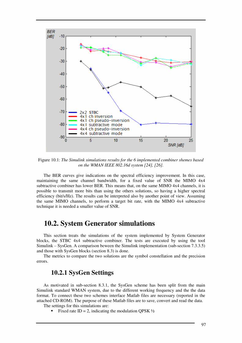
97
Figure 10.1: The Simulink simulations results for the 6 implemented combiner shemes based
on the WMAN IEEE 802.16d system [24], [26].
The BER curves give indications on the spectral efficiency improvement. In this case,
maintaining the same channel bandwidth, for a fixed value of SNR the MIMO 4x4
subtractive combiner has lower BER. This means that, on the same MIMO 4x4 channels, it is
possible to transmit more bits than using the others solutions, so having a higher spectral
efficiency (bit/s/Hz). The results can be interpreted also by another point of view. Assuming
the same MIMO channels, to perform a target bit rate, with the MIMO 4x4 subtractive
technique it is needed a smaller value of SNR.
10.2. System Generator simulations
This section treats the simulations of the system implemented by System Generator
blocks, the STBC 4x4 subtractive combiner. The tests are executed by using the tool
Simulink – SysGen. A comparison beween the Simulink implementation (sub-section 7.3.3.5)
and those with SysGen blocks (section 8.3) is done.
The metrics to compare the two solutions are the symbol constellation and the precision
errors.
10.2.1 SysGen Settings
As motivated in sub-section 8.3.1, the SysGen scheme has been split from the main
Simulink standard WMAN system, due to the different working frequency and the the data
format. To connect these two schemes interface Matlab files are necessary (reported in the
attached CD-ROM). The purpose of these Matlab files are to save, convert and read the data.
The settings for this simulations are:
� Fixed rate ID = 2, indicating the modulation QPSK ½

98
� Fixed SNR [dB] = 25
� Simulation duration = 0.0574 s , equivalent to the transmission of 200 bursts of 4
symbols each.
� STBC MIMO 4x4 subtractive combiner
� Every constraints defined in the common settings in sub-section 10.1.1
10.2.2 SysGen results
The simulations have been done on the same environment as those in section 10.1
(computer in the Embedded Laboratory of the Electronic Systems Department, AAU). It is
expected a decrease of the quality (in terms of accuracy errors) due to the data format
reduction from Simulink double (64-bit) to 8-bit fixed point. The first comparison is
decidedly visual, between the two constellation plots of the same transmitted burst, it is
shown in Figure 10.2.

99
Figure 10.2: The same arbitrary burst transmitted by the Simulink 64-bit STBC MIMO 4x4
subtractive combiner (on the top) and those transmitted by the SysGen impl. (on the bottom).
Figure 10.2 shows the two constellation plots, which are obtained by transmitting with the
STBC MIMO 4x4 subtractive combiner the same arbitrary burst. On the top those
implemented by 64-bit Simulink blocks and on the bottom those designed by the 8-bit
SysGen blocks. It was expected a higher difference between the two plots, but the
transmision by the 8-bit solution, at SNR 25 dB does not introduce errors. By visual
comparison of Figure 10.2, the 8-bit system is close to the 64-bit implementation.
The second metric to compare the two implementations (with Simulink and SysGen) is
looking at the precision errors. The simulation provides 200 bursts from both the schemes, so
subtracting the two data it is possible to have indications about the introduced error. In
particular, split real and imaginary parts are subtracted, considering the unsigned values. The
mean precision errors are indicated in Table 10.1.
Mean Relative Error for Real part Mean Relative Error for Imaginary part
8.68 % 8.72 %
Table 10.1: The mean relative errors introduced by the bit reduction between Simulink and
SysGen implementations.
The mean relative errors introduced by the 8-bit precision of the SysGen implementation
are justified by the considerable reduction of bits. Anyway in the case of QPSK the 8-bit
SysGen implementation does not introduce errors. Due to that, a worse case is proposed in
Appendix C: a 16-QAM ¾ modulation maintaining SNR = 25 dB. For this case is valid the
same discussion.
10.3. SW/HW co-simulation
In this section the SW/HW co-simulation is treated. At first a short description of the
testing environment is proposed. The second sub-section reports the results starting with the
comparison between the SysGen Resource Estimator calculation and the real resources from
the VHDL file (generated by SysGen for the target FPGA, section 9.2.3). A short discussion
about the FPGA working frequency is explained. Finally a consideration about the precision
errors is done.
10.3.1 Environment description
The SW/HW co-simulation is supported by the following tools (reproposed from section
9.2.3), the board ML506 and the connection cables:
� Matlab version 7.6.0.324 (R2008a), from [30]
� Simulink 7.1.1. (R2008a+) from [30]
� Xilinx ISE Design Suite 11.1 (including System Generator for DSP 11.1).
Documentation in [31], [32]
� ML506 platform for Virtex 5 xc5vsx50t-1ff1136 [29]
� Ethernet cable
� USB-JTAG cable
� Power supply
� Computer from the Embedded Laboratory of the Electronic Systems Department,
AAU (performance 2 GHz single core, 1 Gbyte RAM)
In Appendix D section 2 there is a picture of the co-simulation environment.

100
10.3.2 Hardware and Co-simulation results
In this sub-section the hardware resource analysis is reported. Two results are compared,
those from the SysGen Resource Estimator tool and the real amount of FPGA resources
obtained by the VHDL file generation.
Figure 10.3 shows the Resource Estimator results.
Figure 10.3: The results of the Resource Estimator tool. This SysGen functionality gives an
indication on the number of slices, Flip-Flops, Block RAMs, Look up tables, bits of I/Os,
Embedded multipliers (DSP48E) and Buffers..
According with section 8.4 the SysGen combiner which has implemented respects all the
various resources.
In Figure 10.4 the result from the VHDL code generated by the SysGen synthesis is
shown.
Figure 10.4: The results of the VHDL synthesis. The resources considered are the number of
slice/slice registers, Flip-Flops, Memory usage, bits of I/Os, Embedded multipliers (DSP48E)
and Buffers.
Comparing the two results of Figure 10.3 and 10.4, some values are close, as the number
of Flip-Flops-LUTs, the number of bits for I/O, the DSP48E Embedded multipliers and the
Buffers. Other values are not similar, as the number of slices, and the Memory usage. These
differences are justified by the over-estimation of the SysGen Resource Estimation tool,
which assign pre-defined numbers of resources for each SysGen block. Moreover the
computation of Resource Estimator does not consider the pipelining of the operators and the
optimizations done by the VHDL (or bit-stream) synthesis-generator.

101
Looking at Figure 10.4 it is possible to conclude that every limitation is respected, with
the 57 % of area occupation (slices). The most critical value, as expected by the consideration
of sub-section 8.3.1, is the number of bonded I/O, which is at the 80 % of usage. This can be
the main problem if it is wanted to extend the hardware implementation. The number of
DSP48E embedded multipliers is at 88 % but it is not so critical, because the multipliers can
be implemented also by standard slices, so the number of multipliers can be (within reason)
incremented.
Another typical parameter is the working frequency of the system on FPGA. The co-
simulation generation tool has allowed the using of 10 ns FPGA clock period, the maximum
available by System Generator.
The longest path of the system implemented on FPGA is almost at the allowed limit
(from the xflow.results file):
� FPGA clock period (co-simulation) = 10 ns
� Longest path = 9.986 ns
The time slack for this implementation is just 14 ps, that means the impossibility of
adding at the design cascade other combinatorial operators. This, of course without
introducing intermediate registers.
About that, can be usefull to analyze the trade-off between latency and delay. The latency
is the time needed to complete a cascade of combinatorial operations (in this case equal to the
longest path). The delay is the aditional time introduced by sequential devices (as registers).
Analyzing this trade-off is possible to reduce the total execution time, depending on the case.
Figure Figure 10.5 shows an example where would be useful inserting a register and split the
combinatorial part.
Figure 10.5: Example of utility of inserting Register splitting the combinatorial logic.
Figure 10.5 shows a case where can be useful to insert a resister in the middle of a
combinatorial cascade. In fact, keeping the original scheme, would be necessary to increase
the FPGA clock period, which often can assume standard values (i.e. 10 ns, 30 ns or 50 ns).
The increase of the FPGA clock period can slow down the system more than inserting a
register with delay = 1 clock period. For instance, assuming the possible FPGA clock periods
10ns, 30 ns or 50 ns, and that the combinatorial part needs 14 ns to be process. It is not
possible to implement the hardware system at clock 10 ns, but at least 30 ns. The best
solution would be to insert a register in the middle of the combinatorial logic splitting in two
part of 7 ns longest path. Keeping 10 ns of FPGA clock period, the total ime to perform the
same logic would be 20 ns instead of 30 ns.
In this project case the combinatorial logic needs less than the minimum FPGA clock
period for the target Virtex 5 xc5vsx50t, so additional registers are not needed.
The last comparison is done between the SysGen implementation and the FPGA design.
The co-simulation tests have been shown that the two output are exactly the same as expected.
REG REG
COMBINATORIAL LOGIC
Register insertion
10 ns FPGA clock line

102
Figure 10.6: The Rugby Meta-model of this report, On-chip receiver part.

103
11. Conclusion
The purpose of this project was to identify which type of algorithmic improvements can
be used to increase the spectral efficiency of an OFDM/MIMO receiver, while maintaining its
HW feasibility.
In this report, the designer propose a possible solution to the problem statement. This is
the identification of two new techniques, which are conceived to solve the central problem of
the MIMO with more than two transmitting antennas: the quasi-orthogonality of product
between channel matrix and its Hermitian.
This report contains the implementation steps in order to converge to a feasible hardware
solution, starting from the initial problem to the final simulations and SW/HW co-simulation.
The simulations have been divided into three parts. Those concerning the Simulink
implementation, the System Generator design by a hardware point of view, and the co-
simulation tests. The first results show the behavior of the various MISO/MIMO combiner in
a fixed environment. In particular the BERs on SNR characteristics have been plotted. The
results have indicated the subtractive technique as better than the other proposed. This fully
meets the expectations and the estimations which have been done in Chapter 6. In fact the
MIMO 4x4 with subtractive combiner has been identified as those with smaller normalized
noise respect to the pseudo-inversion combiner. The Simulink simulations has indicated the
MIMO 4x4 subtractive combiner as the more performing between the others, in terms of BER
and spectral efficiency. This has justified the choice for the hardware implementation.
The System Generator scheme simulation has shown the limits of the following hardware
implementation. In fact, the bit reduction from 64 to just 8-bit introduces precision errors.
These relative errors are less than the 10 % of the mean 64-bit values for the modulations
BPSK and QPSK, while it is more than 14 % when the modulation is 16-QAM or 64-QAM.
These results are comforting considering the high reduction of bits from 64 to 8.
The last part concerns the SW/HW co-simulation, starting with a comparison between the
SysGen Resource Estimator tool and the real implementation. As expected the values from
the SysGen tool were inaccurate. In particular the number of estimated slices was ca. 12,500
and those from the VHDL file was ca. 4,700. This due to the optimization performed by the
System Generator compiler and automatic pipelining which the Resource Estimator tool does
not consider. The most critical aspect has been identified in the number of available I/O. In
fact, it is difficult to implement parallel architectures if the number of inputs is not
proportioned to the FPGA size. This orientates the future implementations towards solutions
in the middle of the area/execution time trade-off.
The longest path of the hardware implementation is at the limit of the 10 ns FPGA clock
period. This avoids the insertion of additional registers and the splitting of the combinatorial
logic. Finally, the 8-bit FPGA computation shows a perfect meeting with the System
Generator calculation (done by the computer). In fact the relative error is equal to zero.
This report shows a possible solution on which type of algorithmic improvements can be
used to increase the spectral efficiency of an OFDM/MIMO receiver, while maintaining its
HW feasibility.
This report has been organized in three main parts, identified by three keywords, Analysis,
Design and Evaluation. The first part starts with the introduction chapter, that contains this
project context, and it focuses on the problem statement. It follows the chapter concerning the
methodologies and methods. In this, a comparison between various methodologies has been
reported, with the final choise for Rugby Meta-Model [4], [6]. The third chapter consists in
the theoretical overview related to this project, with sub-sections on OFDM and MIMOs.
The second part is the Design and is divided in steps following Rugby Meta-Model. The
initial idea presents the proposed solution for this project. Chapter 5 indicates the cost
function and the other constraints. The sixth chapter contains the system analysis and

104
proposes two new algorithms for QO-MIMO receivers. The following chapter illustrates the
Simulink implementation of the proposed techniques. Chapter 8 focuses on one of these
techniques reporting the development of the System Generation implementation. Finally,
Chapter 9 treats the hardware implementation by a co-simulation point of view.
The last part, Evaluation, starts with the Results chapter. It contains the presentation and
the discussion on the partial and final simulations. Moreover it treats the SW/HW co-
simulation using the target FPGA. Chapter 11 is the conclusion and the proposed future
implementation starting from the work done in this project.
11.1. Future Works
11.1.1. Short time The system implemented in this project is characterized by a complete design flow,
starting from the initial idea and the algorithm definition, through the software and finally to
the hardware implementation. This approach has been supported by the Rugby Meta-Model
and allows to explore the various possible solution step by step, thanks also to the domain
definition (computation, communication, data, time). On the other hands, the various trade-
offs force the designer to make development chice showing also different possible solutions
to solve the initial problem. This provide several alternative ideas or possible optimizations.
Some ideas for possible short time integration/optimization, starting from this
implementation:
� Including more parts on the target FPGA, analyzing the feasibility. The blocks
that can be additionally implemented are:
o the channels estimators
o the blocks for interference subtraction.
� Possible optimization:
o analyze the feasibility of slowing down the execution time and reduce the
resource usage. � drow-back: additional registers which need resources;
11.1.2. Long time Others ideas for future implementation are listed. These solutions needs more time to be
developed, so have been classified as long-time works:
� Realize a real time co-simulation with a single scheme WMAN standard-SysGen
blocks, by using more performing computer/s;
� Replace the FPGA platform with one more performing and conceive a system
with more antennas;
� Explore the possibility to implement the MIMO combiner on a DSP or other
architectural solutions;
� Identify the possibility of blocks for dynamic partial reconfiguration.

105
Bibliography
[1] Luigi Paura, “Wireless Network: state of art and perspectives”, Multimedia
Communications Laboratory of Naples – CNIT. Course slides. December 2004.
[2] ASPI Introduction Slides, Aalborg University, March 2006, “http://kom.aau.dk/
~dsp/aspi05-2/sites/aspi9/OO-Intro-ASPI9-05.ppt282”. Autumn 2005.
[3] Daniel D. Gajski and Robert Kuhn, “Guest Editor’s Introduction: New VLSI Tools”,
IEEE Computer, December 1983, pages 11-14.
[4] Axel Jantsch, Shashi Kumar, Ahmed Hermani, “The Rugby Meta-Model”, Royal
Institute of Technology, Department of Electronics, Kista, Sweden. March 2000.
[5] Kulkarni G., Chitti S. H., Popp A., Le Moullec Y., “ATtACk – A Methodology for
Realiziong Partially Reconfigurable FPGA Systems”, Center for Software Defined
Radio, Department of Electronic Systems Alborg University, IEEE, 2007.
[6] Jantsch A., Kumar S., Hermani A., “The Rugby Model: A Framework for the study
of Modelling, Analysis, and Synthesis Concepts in Electronic Systems”, Proceedings
of Design Automation and Test in Europe (DATE), 1999.
[7] A. Gerstlauer, R. Doemer, J. Peng, Daniel D. Gajski “System Design: A Pratical
Guide with SpecC”, Kluwer Academic Publishers, Chapter 2.
[8] J. N. Latta “Covering Next Generation Compiuting and Communications
Technologies, OFDM Tutorial”, Wave Report,
http://www.wave-report.com/tutorials/OFDM.htm
[9] H. Schulze and C. Lueders, “Theory and Applications of OFDM and CDMA”, John
Wiley & Sons, 2005.
[10] B. Sklar, “Digital Communications: Fundamentals and Applications”, Pearson,
January 2001.
[11] J. G. Proakis, “Digital Communications”, Mc Graw Hill, 2001.
[12] http://www.cnx.org/content/m11762/latest
[13] D. Tse & P. Viswanath, “Fundamentals of Wireless Communication”, Cambridge
University Press, 2005.
[14] A. Bahai, A. J. Goldsmith, S. Cui, “Energy-efficiency of MIMO and cooperative
MIMO techniques in sensor networks”, IEEE Journal on Selected Areas in
Communications, Volume 22, Issue 6, August 2004, pages 1089-1098.
[15] http://en.wikipedia.org/wiki/File:Prinzip_MIMO.png
[16] G. J. Foschini, “Layered Space-Time Architecture for Wireless Communication in a
Fading Environment When Using Multi-Element Antennas”, Bell Labs Technical
Journal, Autumn 1996.
[17] C. Dietrich Jr., “Adaptive Arrays and Diversity Antenna Configurations for Handheld
Wireless Communication Terminals”, 15th February 2000.
[18] H. Wang, et. Al, “Managing dynamic reconfiguration on MIMO Decoder”, IPDPS
2007, pp1-8.
[19] M. Filippi, “Software Defined Radio Implementation of a MIMO Receiver with two
switchable modes”, group 946 ASPI, 9th semester 2008 project report, AAU.
[20] S. M. Alamouti, “A simple transmit diversity tecnique for wireless communications”,
IEEE journal on select areas in communications, vol. 16, no. 8, october 1998.
[21] J. Kim, S. L. Ariyavistajul, “Optimum 4-Transmit-Antenna STBC/SFBC with Angle
Feedback and a Near-Optimum 1-Bit Feedback Scheme”, IEEE Communications
Letters, vol. 11, no. 11, November 2007.
[22] B. Badic, M. Rupp and H. Weinrichter, “Adaptive Channel-Matched Extended
Alamouti Space-Time Code Exploiting Partial Feedback”, ETRI Journal, Volume 26,
no.5, October 2004.
[23] J. Kim, S. L. Ariyavistajul and N. Seshadri, “STBC/SFBC for 4 Transmit Antennas
with 1-bit Feedback”, IEEE Communication, 2008.
[24] IEEE Standard 802.16-2004, “Part 16:Air interface for fixed broadband wireless
access systems”, October 2004, http://ieee802.org/16/published.html.

106
[25] Documentation on WMAN standard, http://wirelessman.org/published.html. (Viewed
on 23/04/09).
[26] The MathWorks Inc., “IEEE 802.16-2004 OFDM PHY Link, Including Space-Time
Block Coding”, 2007-2008 published with Matlab 7.7.
[27] C. Eklund et. al., “WirelessMAN: Inside the IEEE 802.16 Standard for Wireless
Metropolitan Area Networks”, IEEE Press, 2006.
[28] Documentation, Data sheet Virtex 5 FPGA series. (Last visit the 21/03/09).
http://www.xilinx.com/support/documentation/data_sheets/ds100.pdf.
[29] Documentation, Data sheet ML506 board. (Last visit the 21/03/09).
http://www.xilinx.com/support/documentation/boards_and_kits/ug347.pdf.
[30] Official web site of Matlab, http://www.mathworks.com. (Last visit the 02/04/09).
[31] Documentation, manual for System Generator for DSP. (Last visit the 02/04/09).
http://www.xilinx.com/support/documentation/sw_manuals/sysgen_ref.pdf.
[32] Slides, co-simulation ML506 board. (Last visit the 27/04/09).
http://www.xilinx.com/products/boards/ml506/docs/ml506_sysgen_dsp_hw_cosim_...
creation.pdf.
[33] N. Shirazi, J. Ballagh, “Put Hardware in the loop with Xilinx System Generator for
DSP”, Xcell Journal, Fall 2003, http://china.xilinx.com/publications/xcellonline/...
xcell_47/xc_pdf/xc_sysgen47.pdf
[34] Documentation on matrix inversion calculation. (Last visit the 18/04/09).
http://www.cvl.iis.u-tokyo.ac.jp/~miyazaki/tech/teche23.html
[35] Documentation on pseudo-inverse calculation. (Last visit the 18/04/09).
http://profs.sci.univr.it/~fusiello/teaching/visione/vis_art/node23.html
[36] Documentation of Xilinx for Partial Reconfiguration,
www.xilinx.com/support/documentation/application_notes/xapp290.pdf

107
Appendix A
Matlab, Simulink and System Generator
Figure 1: The Matlab windows framework, with 1) the current directory files, 2) the editor for
the matlab code functions and .m files, 3) the workspace indicator of the variable in memory,
4) the command window.

108
Figure 5.2: The Simulink windows framework, with the libraries available on the left, with the
standard blocks window on the centre and the graphic window on the right.
Figure 5.3: The Simulink windows framework with the Xilinx libraries on the left, a scheme
using Xilinx System Generator blocks on the right.

109
Appendix B
1. Matlab code MIMO 2x2 combiner (sub-section 7.2.2)
function z = stbcdec(chEst1,rx1,chEst2,chEst3,rx2,chEst4) % STBCDEC Space-Time Block Combiner %
N = 2; M = 1; z = complex(zeros(size(rx1))); z0 = complex(zeros(size(rx1,1), M)); z1 = z0;
% Space Time Combiner for i = 1:size(rx1,2)/2 z0(:, M) = rx1(:, 2*i-1).* conj(chEst1(:, 2*i-1)) + ... conj(rx1(:, 2*i)).* chEst2(:, 2*i) + ... rx2(:, 2*i-1).* conj(chEst3(:, 2*i-1)) + ... conj(rx2(:, 2*i)).* chEst4(:, 2*i);
z1(:, M) = rx1(:, 2*i-1).* conj(chEst2(:, 2*i-1)) - ... conj(rx1(:, 2*i)).* chEst1(:, 2*i) + ... rx2(:, 2*i-1).* conj(chEst4(:, 2*i-1)) - ... conj(rx2(:, 2*i)).* chEst3(:, 2*i);
z(:, [2*i-1 2*i]) = [z0 z1]; end
2. Matlab code STBC 4x_ encoder (subsection 7.3.1)
function [ant1, ant2, ant3, ant4] = stbcenc(u) % STBCENC Space-Time Block Encoder % Outputs the Space-Time block encoded signal per antenna.
N = 4; ant1 = complex(zeros(size(u))); ant2 = ant1; ant3 = ant1; ant4 = ant1;
% Alamouti Space-Time Block Encoder, G2, full rate % G2 = [s1 s2 s3 s4; s2* -s1* s4* -s3*; s3* s4* -s1* -s2*; s4 -s3
-s2 s1] for i = 1:size(u,2)/4 s1 = u(:, 4*i-3); s2 = u(:, 4*i-2); s3 = u(:, 4*i-1); s4 = u(:, 4*i); ant1(:, [4*i-3 4*i-2 4*i-1 4*i]) = [s1 conj(s2) conj(s3) s4]; ant2(:, [4*i-3 4*i-2 4*i-1 4*i]) = [s2 -conj(s1) conj(s4) -s3]; ant3(:, [4*i-3 4*i-2 4*i-1 4*i]) = [s3 conj(s4) -conj(s1) -s2]; ant4(:, [4*i-3 4*i-2 4*i-1 4*i]) = [s4 -conj(s3) -conj(s2) s1]; end

110
3. Channel inversion 4x1 combiner (sub-section 7.3.3.1)
Matrix inversion
function zagg1 = inversion(ch3,ch1, ch2,ch4) % Variable definition
zagg = complex(zeros(200,4)); zagg1 = complex(zeros(200,16)); zinv = complex(zeros(800,4)); % Four channel estimations are put in the channel matrix H (zagg 4x4)
% Zagg is inverted to zinv (4x4)
for i = 1:50 zagg(4*i-3,:) = [ch1(i,1) ch2(i,1) ch3(i,1) ch4(i,1)]; zagg(4*i-2,:) = [-conj(ch2(i,1)) conj(ch1(i,1)), -conj(ch4(i,1))
conj(ch3(i,1))]; zagg(4*i-1,:) = [-conj(ch3(i,1)), -conj(ch4(i,1)) conj(ch1(i,1))
conj(ch2(i,1))]; zagg(4*i,:) = [ch4(i,1), -ch3(i,1), -ch2(i,1) ch1(i,1)]; zinv([4*i-3 4*i-2 4*i-1 4*i],:) = inv(zagg([4*i-3 4*i-2 4*i-1
4*i],:)); end % reshape the channel inverted matrix for the STBC combiner (4x16) for i = 1:50 zagg1(4*i-3,1:16) = [zinv(4*i-3,1:4) zinv(4*i-2,1:4) zinv(4*i-
1,1:4) zinv(4*i,1:4)]; zagg1(4*i-2,1:16) = [zinv(4*i-3,1:4) zinv(4*i-2,1:4) zinv(4*i-
1,1:4) zinv(4*i,1:4)]; zagg1(4*i-1,1:16) = [zinv(4*i-3,1:4) zinv(4*i-2,1:4) zinv(4*i-
1,1:4) zinv(4*i,1:4)]; zagg1(4*i,1:16) = [zinv(4*i-3,1:4) zinv(4*i-2,1:4) zinv(4*i-
1,1:4) zinv(4*i,1:4)]; end
MISO combiner
function z = stbcdec(chEstinv, rx) % STBCDEC Space-Time Block Combiner for channel inversion N = 4; M = 1; z = complex(zeros(size(rx))); z0 = complex(zeros(size(rx,1), M)); z1 = z0; z2 = z0; z3 = z0; for i = 1:size(rx,2)/4 z0(:, M) = rx(:, 4*i-3).* chEstinv(:, 1) + ... conj(rx(:, 4*i-2)).* chEstinv(:, 2) + ... conj(rx(:, 4*i-1)).* chEstinv(:, 3) + ... rx(:, 4*i).* chEstinv(:, 4); z1(:, M) = rx(:, 4*i-3).* chEstinv(:, 5) + ... conj(rx(:, 4*i-2)).* chEstinv(:, 6) + ... conj(rx(:, 4*i-1)).* chEstinv(:, 7) + ... rx(:, 4*i).* chEstinv(:, 8); z2(:, M) = rx(:, 4*i-3).* chEstinv(:, 9) + ... conj(rx(:, 4*i-2)).* chEstinv(:, 10) + ... conj(rx(:, 4*i-1)).* chEstinv(:, 11) + ... rx(:, 4*i).* chEstinv(:, 12); z3(:, M) = rx(:, 4*i-3).* chEstinv(:, 13) + ... conj(rx(:, 4*i-2)).* chEstinv(:, 14) + ... conj(rx(:, 4*i-1)).* chEstinv(:, 15) + ... rx(:, 4*i).* chEstinv(:, 16); z(:, [4*i-3 4*i-2 4*i-1 4*i]) = [z0 z1 z2 z3]; end

111
4. Pseudo-inversion 4x1 combiner (sub-section 7.3.3.2)
function zagg1 = pseudoinversion(ch3,ch1,ch2,ch4) zagg = complex(zeros(200,4)); zt = complex(zeros(4,4)); zagg1 = complex(zeros(200,16)); zinv = complex(zeros(800,4)); for i = 1:50 zagg(4*i-3,:) = [ch1(i,1) ch2(i,1) ch3(i,1) ch4(i,1)]; zagg(4*i-2,:) = [-conj(ch2(i,1)) conj(ch1(i,1)), -conj(ch4(i,1))
conj(ch3(i,1))]; zagg(4*i-1,:) = [-conj(ch3(i,1)), -conj(ch4(i,1)) conj(ch1(i,1))
conj(ch2(i,1))]; zagg(4*i,:) = [ch4(i,1), -ch3(i,1), -ch2(i,1) ch1(i,1)]; zt = transpose(zagg([4*i-3 4*i-2 4*i-1 4*i],:)); zinv([4*i-3 4*i-2 4*i-1 4*i],:) = inv(zt*zagg([4*i-3 4*i-2 4*i-1
4*i],:))*zt; end for i = 1:50 zagg1(4*i-3,1:16) = [zinv(4*i-3,1:4) zinv(4*i-2,1:4) zinv(4*i-
1,1:4) zinv(4*i,1:4)]; zagg1(4*i-2,1:16) = [zinv(4*i-3,1:4) zinv(4*i-2,1:4) zinv(4*i-
1,1:4) zinv(4*i,1:4)]; zagg1(4*i-1,1:16) = [zinv(4*i-3,1:4) zinv(4*i-2,1:4) zinv(4*i-
1,1:4) zinv(4*i,1:4)]; zagg1(4*i,1:16) = [zinv(4*i-3,1:4) zinv(4*i-2,1:4) zinv(4*i-
1,1:4) zinv(4*i,1:4)]; end
5. Subtractive 4x1 combiner (sub-section 7.3.3.3)
function [z,zinv] = subtractivedec(chEst3,chEst1,rx,chEst2,chEst4) % STBCDEC Space-Time Block Combiner for the subtractive technique N = 4; M = 1; z = complex(zeros(size(rx))); zinv = z; z0 = complex(zeros(size(rx,1), M)); z1 = z0; z2 = z0; z3 = z0; for i = 1:size(rx,2)/4 z0(:, M) = rx(:, 4*i-3).* conj(chEst1(:, 4*i-3)) - ... conj(rx(:, 4*i-2)).* chEst2(:, 4*i-2) - ... conj(rx(:, 4*i-1)).* chEst3(:, 4*i-1) + ... rx(:, 4*i).* conj(chEst4(:, 4*i)); z1(:, M) = rx(:, 4*i-3).* conj(chEst2(:, 4*i-3)) + ... conj(rx(:, 4*i-2)).* chEst1(:, 4*i-2) - ... conj(rx(:, 4*i-1)).* chEst4(:, 4*i-1) - ... rx(:, 4*i).* conj(chEst3(:, 4*i)); z2(:, M) = rx(:, 4*i-3).* conj(chEst3(:, 4*i-3)) - ... conj(rx(:, 4*i-2)).* chEst4(:, 4*i-2) + ... conj(rx(:, 4*i-1)).* chEst1(:, 4*i-1) - ... rx(:, 4*i).* conj(chEst2(:, 4*i)); z3(:, M) = rx(:, 4*i-3).* conj(chEst4(:, 4*i-3)) + ... conj(rx(:, 4*i-2)).* chEst3(:, 4*i-2) + ... conj(rx(:, 4*i-1)).* chEst2(:, 4*i-1) + ... rx(:, 4*i).* conj(chEst1(:, 4*i)); z(:, [4*i-3 4*i-2 4*i-1 4*i]) = [z0 z1 z2 z3]; zinv(:, [4*i-3 4*i-2 4*i-1 4*i]) = [-z3 z2 z1 -z0]; end

112
6. Pseudo-inversion 4x4 combiner (sub-section 7.3.3.4)
…
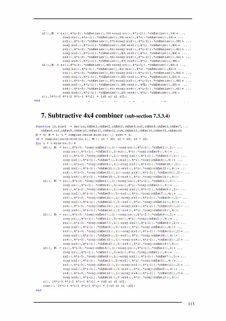
113
…
7. Subtractive 4x4 combiner (sub-section 7.3.3.4)

114

115
Appendix C
The SysGen simulation, 16-QAM¾ (sub-section 10.2.2)
The same arbitrary burst transmitted by the Simulink 64-bit STBC MIMO 4x4 subtractive
combiner (on the top) and those transmitted by the SysGen impl. (on the bottom).
Mean Relative Error for Real part Mean Relative Error for Imaginary part
14.2 % 14.4 %
The mean relative errors introduced by the bit reduction between Simulink and SysGen
implementations.

116
Appendix D
1. The ML506 platform picture (section 9.1.)
2. The Co-simulation environment (sub-section 10.3.1)


![Hard Decision-Based PWM for MIMO-OFDM Radar · 2. MIMO-OFDM Radar Signal Model-Based PWM 2.1. MIMO-OFDM Radar Systems Structure In [1], OFDM technique has the advantage of combating](https://img.dokumen.tips/doc/110x75/5e6a685a5002aa073940e3bf/hard-decision-based-pwm-for-mimo-ofdm-radar-2-mimo-ofdm-radar-signal-model-based.jpg)