Embed Size (px)
Citation preview
34
Maarit Laaksonen
RESE
ARCH Population Attributable
Fraction (PAF) in Epidemiologic Follow-up Studies

Maarit Laaksonen
Population Attributable Fraction (PAF) in Epidemiologic Follow-up
Studies
A c A d e M i c d i s s e r t A t i o n
to be presented with the permission of the Faculty of Medicine of the University of tampere, for public examination in the Auditorium
of the tampere school of Public Health Medisiinarinkatu 3, tampere, on June 18, 2010, at 12 o’clock noon.
national institute for Health and Welfare, Helsinki, Finland
and
tampere school of Public Health, University of tampere, Finland
reseArcH 34Helsinki 2010

© Maarit Laaksonen and National Institute for Health and Welfare
Cover: Textile art by Maiju Ahlgrén, photographed by Timo Seppälä Layout: Riitta Nieminen
ISBN 978-952-245-303-7 (printed) ISSN 1798-0054 (printed)ISBN 978-952-254-304-4 (pdf)ISSN 1798-0062 (pdf)
Helsinki University PrintHelsinki, Finland 2010
S u p e r v i s e d b y
Research Professor Paul Knekt, PHDDepartment of Health, Functional Capacity and Welfare
National Institute for Health and Welfare Helsinki, Finland
Academy Professor Hannu Oja, PhDTampere School of Public Health
University of TampereFinland
Doctor Tommi Härkänen, PhDDepartment of Health, Functional Capacity and Welfare
National Institute for Health and Welfare Helsinki, Finland
R e v i e w e d b y
Professor Seppo Sarna, PhDDepartment of Public Health
University of HelsinkiFinland
Professor Esa Läärä, LSocSc Department of Mathematical Sciences
University of OuluFinland
O p p o n e n t
Research Professor Kari Kuulasmaa, PhDDepartment of Chronic Disease Prevention
National Institute for Health and WelfareHelsinki, Finland

To my Dad
6 Research 34/2010National Institute for Health and Welfare
Population Attributable Fraction (PAF) in Epidemiologic Follow-up Studies
ABSTRACT
Maarit Laaksonen. Population Attributable Fraction (PAF) in epidemiologic follow-up studies. National Institute for Health and Welfare (THL), Research 34, 150 Pages. Helsinki, Finland 2010. ISBN 978-952-245-303-7 (printed); ISBN 978-952-254-304-4 (pdf)
Quantification of the impact of exposure to different risk factors on mortality or morbidity at the population level is a fundamental issue in epidemiologic research. Population Attributable Fraction (PAF) is a statistical concept that can be used to quantify this impact. PAF assesses the proportion of outcome that could be avoided if the current exposure distribution was replaced by a hypothetical, presumably preferable exposure distribution. So far, the methods for the estimation of PAF have been developed for and applied in case-control and cross-sectional studies. The development of methods for the estimation of PAF from cohort studies, which properly take into account the time perspective, has started only recently. In the estimation of PAF for a certain follow-up time interval, the type of outcome of interest (mortality vs. morbidity) has not, however, been taken into account. In this study, the statistical methodology for the estimation of PAF in cohort studies will be extended to cover both the estimation of PAF for total mortality and disease incidence.
The PAF for total mortality or disease incidence was defined as the proportion of mortality or disease incidence, respectively, that could be avoided during a follow-up time interval (0, t] if their risk factors were modified. A parametric proportional hazards model, with a piecewise constant baseline hazard function for death and disease occurrences, was assumed. Potential confounding factors were adjusted for and potential effect modifying factors accounted for in the model. The estimation of PAF and its asymptotic variance based on the delta method was demonstrated. The complementary logarithmic transformation in the calculation of the confidence interval of PAF was used. In the estimation of PAF for total mortality, only censoring due to loss to follow-up was taken into account, whereas in the estimation of PAF for disease incidence censoring due to death was also considered. Furthermore, the meta-analysis techniques developed for pooling of relative risks were extended for the pooling of PAF estimates. In the data examples of this study, the PAF estimates for total mortality and disease incidence were demonstrated to decrease as the follow-up time increased. In the simulated data sets, taking censoring due to death into account in the estimation of PAF for disease incidence was shown to decrease the point estimates of PAF significantly in comparison to when censoring due to death was ignored. Ignoring censoring due to

7Research 34/2010National Institute for Health and Welfare
Population Attributable Fraction (PAF) in Epidemiologic Follow-up Studies
death increased the overestimation of PAF, especially when the impact of risk factors on mortality was strong and the follow-up time long.
A new program for the estimation of PAF both for total mortality and disease incidence, implementing the new methods, was developed using SAS/IML language. This program was shown to be flexible and fast. An application of PAF to evaluate the relative importance of the risk factors of type 2 diabetes and the potential effect-modifying role of metabolic syndrome or its components in a meta-analysis of two representative Finnish cohorts was carried out using this program. As a result, the use of PAF provided further evidence of weight control being the primary diabetes prevention method. The pooling of the PAF estimates increased the power to detect associations in smaller subpopulations defined by the metabolic syndrome or its components, establishing new evidence on the importance of early lifestyle changes in the prevention of type 2 diabetes.
In conclusion, it is essential to take time perspective into account in the estimation of PAF. Different estimators of PAF for a certain time interval, taking into account different sources of censoring, are needed, depending on the outcome of interest. PAF is a useful measure in cohort studies for providing population-level information on the effects of predictor modifications on the outcome in time and has wide applications in many different fields of research.
Keywords: Population Attributable Fraction, cohort studies, risk factor, mortality, disease incidence, piecewise constant hazards model, censoring, effect modification, meta-analysis, SAS macro, type 2 diabetes, lifestyle, metabolic syndrome

8 Research 34/2010National Institute for Health and Welfare
Population Attributable Fraction (PAF) in Epidemiologic Follow-up Studies
TIIVISTELMÄ
Maarit Laaksonen. Population Attributable Fraction (PAF) in epidemiologic follow-up studies. [Väestösyyosuus epidemiologisissa seurantatutkimuksissa].Terveyden ja hyvinvoinnin laitos (THL), Tutkimus 34, 150 sivua. Helsinki 2010.ISBN 978-952-245-303-7 (painettu); ISBN 978-952-254-304-4 (pdf)
Eri riskitekijöiden vaikutuksen määrittäminen suhteessa kuolleisuuteen tai sairastu-kutuksen määrittäminen suhteessa kuolleisuuteen tai sairastu-vuuteen väestötasolla on keskeistä epidemiologisessa tutkimuksessa. Väestösyyosuus on tilastollinen tunnusluku, jolla voidaan arvioida eri riskitekijöiden selittämää osuut-ta kuolleisuudesta tai sairastuvuudesta. Väestösyysosuus kuvaa, miten suuri osuus tapahtumista voitaisiin välttää, jos yksi tai useampi riskitekijä voitaisiin poistaa tai sen arvoja parantaa. Menetelmiä väestösyyosuuden arviointiin on tähän asti lähinnä kehitetty ja sovellettu tapaus-verrokki- ja poikkileikkaustutkimuksissa. Menetelmiä väestösyyosuuden arviointiin kohorttitutkimuksista, joissa seurataan tutkitun väestö-ryhmän kuolleisuutta tai sairastuvuutta, on puolestaan ryhdytty kehittämään vasta vii-me vuosina. Arvioitaessa riskitekijöiden selittämää osuutta vasteen ilmaantumisesta tietyllä aikavälillä, vasteen tyyppiä (kuolleisuus vs. sairastuvuus) ei ole kuitenkaan toistaiseksi huomioitu. Tässä työssä kehitetään tilastollisia menetelmiä riskitekijöiden sekä kokonaiskuolleisuudesta että sairastuvuudesta selittämän väestösyyosuuden ar-viointiin kohorttitutkimuksista.
Riskitekijöiden selittämä väestösyyosuus määriteltiin osuudeksi kokonaiskuolleisuu-desta tai sairastuvuudesta, joka voitaisiin välttää aikavälillä (0, t], jos niiden riskite-kijöitä kyettäisiin muuttamaan. Kuolleisuuden ja sairauden ilmaantuvuuden oletettiin noudattavan parametrista suhteellisten hasardien mallia. Potentiaaliset sekoittavat tekijät vakioitiin ja potentiaaliset vaikutusta muokkaavat tekijät huomioitiin malli-tuksessa. Välikohtaisesti tasaisen hasardin mallin mukaisesti perushasardin annet-tiin vaihdella seuranta-aikavälien mukaan. Väestösyyosuuden piste-estimaatin ja sen asymptoottisen varianssin laskenta delta-menetelmään nojautuen esitettiin. Luotta-musvälin laskennassa käytettiin kääntäen logaritmista muunnosta. Riskitekijöiden kokonaiskuolleisuudesta selittämän väestösyyosuuden estimoinnissa huomioitiin seu-rannan päättymisestä johtuva havaintojen oikealta sensuroituminen, kun taas niiden selittämää väestösyyosuutta sairastuvuudesta estimoitaessa huomioitiin myös kuol-leisuudesta johtuva sensuroituminen. Lisäksi tässä työssä laajennettiin eri aineistois-ta laskettujen suhteellisten riskien yhdistämiseen kehitetyt meta-analyysimenetelmät myös eri aineistoista laskettujen väestösyyosuusestimaattien yhdistämiseen. Sovellet-taessa uusia menetelmiä eri aineistoihin osoittautui, että kokonaiskuolleisuuden ja sai-
9Research 34/2010National Institute for Health and Welfare
Population Attributable Fraction (PAF) in Epidemiologic Follow-up Studies
rastuvuuden riskitekijöille saadut väestösyyosuusestimaatit pienenevät seuranta-ajan pidentyessä. Kuolinsensuroinnin huomioiminen riskitekijöiden sairastuvuudesta se-littämää väestösyyosuutta laskettaessa pienensi väestösyyosuusestimaatteja merkittä-västi. Kuolinsensuroinnin huomiotta jättämisestä aiheutuva väestösyyosuuden yliesti-mointi oli sitä merkittävämpää mitä voimakkaampi tutkittavien riskitekijöiden yhteys kuolleisuuteen oli ja mitä pidempi seuranta-aika oli.
Tässä työssä kehitettiin uusi, edellä kuvattuihin tilastollisiin menetelmiin pohjautuva, ohjelma sekä riskitekijöiden kokonaiskuolleisuudesta että sairastuvuudesta selittämän väestösyyosuuden estimointiin. Tämä uusi, SAS/IML-kieleen pohjautuva ohjelma, osoittautui joustavaksi ja nopeaksi. Tätä ohjelmaa käyttäen tutkittiin tyypin 2 diabe-teksen riskitekijöiden suhteellista merkitystä väestötasolla kyseisen sairauden aiheut-tajina kahta suomalaista väestöä edustavan otoksen meta-analyysiin pohjautuen. Li-säksi selvitettiin metabolisen oireyhtymän merkitystä näiden riskitekijöiden ja tyypin 2 diabeteksen välistä yhteyttä mahdollisesti muokkaavana tekijänä. Tämä sovellus toi lisää näyttöä painonhallinnan merkityksestä tyypin 2 diabeteksen tärkeimpänä ehkäi-sykeinona. Näiden kahden aineiston väestösyyosuusestimaattien yhdistämisellä saa-tiin lisää tilastollista voimaa riskitekijöiden ja sairauden välisen yhteyden tutkimiseen mahdollisena vaikutusta muokkaavana tekijänä analysoidun metabolisen oireyhtymän tai sen osakomponenttien arvojen perusteella muodostetuissa osa-aineistoissa. Tällä tavalla kyettiin tuottamaan uutta tietoa varhaisten elintapatekijöiden muutosten ilmei-sestä merkityksestä tyypin 2 diabeteksen ehkäisyssä.
Ajallisen ulottuvuuden huomioiminen väestösyyosuuksia estimoitaessa osoittautui keskeiseksi. Riippuen kiinnostuksen kohteena olevasta tapahtumasta tarvitaan erilai-sia väestösyyosuustunnuslukuja, joissa huomioidaan mahdollinen eri syistä johtuva sensuroituminen tarkasteltavalla aikavälillä. Väestösyyosuus on hyödyllinen mittari, jolla voidaan tuottaa väestötasoista tietoa erilaisten ennustekijöiden vaikutuksesta eri-laisiin vasteisiin ja jolla on laajoja käyttömahdollisuuksia monilla eri tutkimusalueil-la.
Asiasanat: väestösyyosuus, kohorttitutkimukset, riskitekijä, kuolleisuus, sairastuvuus, välikohtaisesti tasaisen hasardin malli, sensuroituminen, vaikutusta muokkaavat tekijät, meta-analyysi, SAS makro, tyypin 2 diabetes, elämäntapa, metabolinen oireyhtymä
10 Research 34/2010National Institute for Health and Welfare
Population Attributable Fraction (PAF) in Epidemiologic Follow-up Studies
ConTEnTS
ABSTRACT .......................................................................................................................6
TIIVISTELMÄ .................................................................................................................8
ABBREVIATIONS .........................................................................................................12
LIST OF ORIGINAL PUBLICATIONS .....................................................................13
1 INTRODUCTION ..................................................................................................14
2 REVIEW OF THE LITERATURE .....................................................................162.1 DefinitionofPopulationAttributableFraction(PAF) .............................162.2 GeneralizationofPAFtoaccountforconfounding ...................................212.3 Model-basedestimationofPAFinacohortstudydesign ........................24
3 AIMS OF THE STUDY .........................................................................................30
4 STATISTICAL METHOD FOR THE ESTIMATION OF PAF IN A COHORT STUDY DESIGN ..............................................................................314.1 DefinitionofPAFinacohortstudydesign ................................................31
4.1.1 General definition of PAF ....................................................................... 314.1.2 Definition of PAF for total mortality ..................................................... 314.1.3 Definition of PAF for disease incidence ................................................32
4.2 Generalmodelassumptions ........................................................................334.2.1 Piecewise constant hazards model .........................................................34
4.3 Model-basedcalculationofPAFinacohortstudydesign .......................354.3.1 Calculation of PAF for total mortality ...................................................354.3.2 Calculation of PAF for disease incidence ...............................................36
4.4 EstimationofPAFinacohortstudydesign ..............................................364.4.1 Estimation of PAF for total mortality ....................................................364.4.2 Estimation of PAF for disease incidence ...............................................39
4.5 EstimationofPAFinacohortstudydesigninthepresence ofpotentialeffectmodification ...................................................................40
4.6 EstimationofPAFinapooledcohortstudydesign ..................................41
5 SAS PROGRAM FOR THE ESTIMATION OF PAF IN A COHORT STUDY DESIGN ...................................................................................................................435.1 Backgroundandobjectives ..........................................................................435.2 Functioningoftheprogram .........................................................................43
11Research 34/2010National Institute for Health and Welfare
Population Attributable Fraction (PAF) in Epidemiologic Follow-up Studies
5.3 Dataexamplebasedonsimulateddata ......................................................455.3.1 Simulation design ...................................................................................455.3.2 PAF analysis ...........................................................................................465.3.3 Results ....................................................................................................47
6 RELATIVE IMPORTANCE OF THE MODIFIABLE RISK FACTORS OF TYPE 2 DIABETES – AN APPLICATION OF PAF ...................................496.1 Populationsandmeasurementmethods .....................................................50
6.1.1 Study populations ....................................................................................506.1.2 Risk assessment ......................................................................................506.1.3 Diabetes incidence ..................................................................................52
6.2 Statisticalmethods .......................................................................................526.2.1 Cohort-specific analyses .........................................................................526.2.2 Pooling .....................................................................................................53
6.3 Results ............................................................................................................536.3.1 Description of the study populations ......................................................536.3.2 PAF for lifestyle factors and components of metabolic syndrome .......566.3.3 Effect modification by metabolic syndrome and socio-demographic
factors .....................................................................................................56
7 DISCUSSION ..........................................................................................................607.1 Mainfindings ................................................................................................60
7.1.1 Statistical method and program for the estimation of PAF for total mortality and disease incidence in a cohort study design ......................60
7.1.2 Application of PAF for the analysis of the relative importance of the risk factors of type 2 diabetes ......................................................62
7.2 Methodologicalconsiderations .....................................................................637.2.1 Statistical method and program for the estimation of PAF for total
mortality and disease incidence in a cohort study design ......................637.2.2 Application of PAF for the analysis of the relative importance
of the risk factors of type 2 diabetes ......................................................677.3 Implicationsforfurtherresearch ..............................................................69
8 CONCLUSIONS ......................................................................................................72
9 ACKNOWLEDGEMENTS ....................................................................................74
10 REFERENCES .......................................................................................................77
APPENDICES .................................................................................................................84

12 Research 34/2010National Institute for Health and Welfare
Population Attributable Fraction (PAF) in Epidemiologic Follow-up Studies
ABBREVIATIonS
AF Attributable Fraction
BMI Body mass index
CI Confidence interval
HDL High-density lipoprotein
Health 2000 Health 2000 Survey
HR Hazard ratio
IDF International Diabetes Federation
MFH Mini-Finland Health Survey
OR Odds ratio
PAF Population Attributable Fraction
PAF(0,t] Population Attributable Fraction for time interval (0, t]
M(0, ]PAF t Population Attributable Fraction for total mortality for time interval (0, t]
D(0, ]PAF t Population Attributable Fraction for disease incidence for time interval (0, t]
PAHF Population Attributable Hazard Fraction
PAHFt Population Attributable Hazard Fraction at time t
PASF Population Attributable Survival Fraction
(0, ]PASF t Population Attributable Survival Fraction for time interval (0, t]
PF Prevented Fraction
RR Relative risk
WHO World Health Organization
13Research 34/2010National Institute for Health and Welfare
Population Attributable Fraction (PAF) in Epidemiologic Follow-up Studies
LIST oF oRIGInAL PUBLICATIonS
This dissertation is based on the following original publications referred to in the text by their Roman numerals:
I Laaksonen MA, Knekt P, Härkänen T, Virtala E, Oja H. Estimation of the Population Attributable Fraction for mortality in a cohort study using a piecewise constant hazards model. American Journal of Epidemiology, 2010; 171(7): 837–847.
II Laaksonen MA, Härkänen T, Knekt P, Virtala E, Oja H. Estimation of Population Attributable Fraction (PAF) for disease occurrence in a cohort study design. Statatistics in Medicine, 2010; 29(7–8): 860–874.
III Laaksonen MA, Virtala E, Knekt P, Oja H, Härkänen T. SAS macros for calculation of Population Attributable Fraction (PAF) in a cohort study design. Submitted.
IV Laaksonen MA, Knekt P, Rissanen H, Härkänen T, Virtala E, Marniemi J, Aromaa A, Heliövaara M, Reunanen A. The relative importance of modifiable potential risk factors of type 2 diabetes: a meta-analysis of two cohorts. European Journal of Epidemiology, 2010; 25(2): 115–124.
These articles are reproduced with the kind permission of their copyright holders.
14 Research 34/2010National Institute for Health and Welfare
Population Attributable Fraction (PAF) in Epidemiologic Follow-up Studies
1 InTRoDUCTIon
Quantification of the impact of exposure to modifiable risk factors on different types of outcome, mortality or a certain disease, at the population level is a fundamental public health issue. In epidemiologic studies, the strength of association between risk factors and an outcome are often reported as relative risks (RR) or odds ratios (OR). These measures do not, however, consider the importance of the risk factor at the population level, as its prevalence is not taken into account. An integrated measure that takes into account both the strength of association between the risk factor and the outcome and the prevalence of the risk factor in the population is needed to provide estimates of the public health importance of the risk factors. Population Attributable Fraction (PAF), which assesses the proportion of outcome in a population attributable to an exposure to one or several risk factors, is this kind of a measure.
The basic idea of PAF is to estimate the proportion of outcome in a given population that would theoretically not have occurred if none of the individuals had been exposed to the risk factor. Since its introduction (Levin 1953), a variety of names and definitions for this concept have been proposed (Uter and Pfahlberg 2001). Despite of this confusion, PAF has gradually become a more widely used measure and the estimation of PAF has been applied in different settings and designs. Originally, PAF was formulated for a single dichotomous risk factor (Levin 1953) and was later extended for multiple, polytomous or continuous risk factors (Miettinen 1974, Walter 1976, Deubner et al. 1980). Initially, PAF estimates ignored confounding factors and were thus generally biased (Levin 1953, MacMahon and Pugh 1970, Miettinen 1974). Later, the different statistical strategies for the adjustment of potential confounding factors in the estimation of PAF, mainly stratification and modeling, have, however, been well covered in the literature (Walter 1976, Bruzzi et al. 1985, Benichou 2001). Modeling has generally been regarded as the most flexible way of adjusting PAF. There is a large body of literature on formulas for the estimation of PAF in case-control and cross-sectional studies, as well as in cohort studies with a fixed follow-up time (Walter 1976, Benichou 2001). The literature on the estimation of PAF in cohort studies with censored time-to-event data, which properly takes into account the follow-up time, is, however, scarce (Chen et al. 2006, Samuelsen and Eide 2008, Cox et al. 2009).
In the existing literature on cohort studies, the type of outcome of interest and its influence on the estimation of PAF has received little attention (Schumacher et al. 2007). So far, mainly censoring due to loss to follow-up has been considered in the estimation

15Research 34/2010National Institute for Health and Welfare
Population Attributable Fraction (PAF) in Epidemiologic Follow-up Studies
1 INtRoductIoN
of PAF. This is sufficient if the outcome is death, whereas in the case of disease incidence censoring due to death should also be taken into account. So far, censoring due to death in the estimation of PAF for disease incidence has only been considered in single studies (Silverberg et al. 2004, Samuelsen and Eide 2008). If the risk factors of the disease of interest are similarly related to mortality, their modification is likely to delay not only the occurrence of the disease but also death. Therefore, the impact of the risk factor modification not only on disease incidence but also on mortality should be taken into account in the estimation of PAF for disease. Thus, two different sets of formulas for the estimation of PAF depending on the outcome of interest are needed in order to obtain accurate and interpretable results. Furthermore, in the existing literature on the estimation of PAF for a certain time interval, the estimation has mainly been based on using the semi-parametric Cox proportional hazards model with the Breslow estimator for the cumulative baseline hazard (Breslow 1974). The variance of PAF has been estimated using asymptotic variance estimation (Chen et al. 2006) or time-consuming resampling-based methods, such as bootstrapping (Samuelsen and Eide 2008). An analytic variance estimate for a fully parametrized model based on the delta method is still missing. In addition, to be able to analyze the impact of some potential effect modifying factor on the relationship between the risk factor and the outcome of interest at the population level, we need to be able to calculate PAF estimates in the different subpopulations defined by categories of the effect modifying factor and study the statistical significance of their differences. Adequate methods for doing this in cohort studies are, however, still missing. As the pooling of different cohorts has become more popular, a need for the estimation of PAF in a pooled cohort study design has arisen. No methodology for their estimation has, however, yet been presented. Presently, there are no publicly available programs for the estimation of PAF in cohort studies for a certain time interval. In order to promote the estimation and the correct use of PAF in public health research, a publicly available program, applicable also for the estimation of PAF for disease occurrence, would thus be needed.
In this study, methods for the estimation of model-based adjusted PAF and its asymptotic variance in a cohort study design both for total mortality and for disease occurrence, which takes into account censoring due to death, will be developed. The analysis of PAF in the presence of potential effect modification is also presented. The use of these methods in a pooled cohort study design will also be demonstrated. Furthermore, a program for the estimation of PAF will be presented. Finally, these methods and the new program are applied to explore the relative importance of potential modifiable risk factors of type 2 diabetes in a pooled data of two cohorts.
16 Research 34/2010National Institute for Health and Welfare
Population Attributable Fraction (PAF) in Epidemiologic Follow-up Studies
2 REVIEW oF THE LITERATURE
2.1 Definition of Population Attributable Fraction (PAF)
Once it has been established that there is a causal association between a risk factor and an outcome, we may wish to ascertain what proportion of the outcome is due to the exposure to the risk factor. Let us consider a binary outcome variable D and a dichotomous risk factor E. Let us denote D2 for the presence (D1 for the absence) of the outcome, and E2 for the presence (E1 for the absence) of exposure to the risk factor. Let 2P(E ) and 2P(D ) then denote the exposure prevalence and the outcome occurrence within the entire population, respectively. Furthermore, let 2 2 2R = P(D | E ) and 1 2 1R = P(D | E ) represent the outcome occurrence in the exposed and unexposed individuals, and 2 1RR = R R the relative risk between the exposed and unexposed individuals. Then, the proportion of the outcomes occurring among the exposed individuals, which is in excess in comparison to the unexposed individuals, can be calculated by dividing the risk difference between the exposed and the unexposed individuals by the risk in the exposed individuals:
(2.1) 2 2 2 1 2 1
2 2 2
P(D | E ) P(D | E ) R R RR 1AFP(D | E ) R RR
− − −= = = .
This quantity is here referred to as the Attributable Fraction (AF), i.e. the proportion of the outcome among the exposed individuals attributable to the given exposure. In the literature, it has also been referred to as attributable risk (MacMahon and Pugh 1970), attributable risk percent (Cole and MacMahon 1971) and etiologic fraction (Miettinen 1974). Miettinen (1974) distinguished between etiologic fraction attributable to or related to a given risk factor depending on whether all or just some confounding by extraneous factors was under control. Greenland and Robins (1988) further distinguished between etiologic fraction and excess fraction depending on whether a case attributable to exposure to a risk factor was defined as a case for which the exposure played an etiologic role, thus making it occur earlier, or a case that would not have occurred had exposure never occurred. The definitions behind the algebraic formulations may thus affect the estimates obtained.
The AF can be generalized to the total population of exposed and unexposed individuals in order to quantify the importance of the exposure at the population level.
17Research 34/2010National Institute for Health and Welfare
Population Attributable Fraction (PAF) in Epidemiologic Follow-up Studies
2 REvIEW oF tHE lItERAtuRE
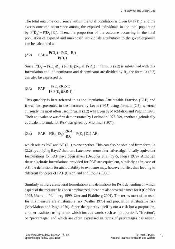
The total outcome occurrence within the total population is given by 2P(D ) and the excess outcome occurrence among the exposed individuals in the total population by 2 2 1P(D ) P(D | E )− . Then, the proportion of the outcome occurring in the total population of exposed and unexposed individuals attributable to the given exposure can be calculated as
(2.2) 2 2 1
2
P(D ) P(D | E )PAFP(D )−= .
Since 2 2 2 2 1P(D ) = P(E )R +(1-P(E ))R , if 2P(D ) in formula (2.2) is substituted with this formulation and the nominator and denominator are divided by R1, the formula (2.2) can also be expressed as
(2.3) 2
2
P(E )(RR-1)PAF1+ P(E )(RR-1)
= .
This quantity is here referred to as the Population Attributable Fraction (PAF) and it was first presented in the literature by Levin (1953) using formula (2.3), whereas currently the most often used formula (2.2) was given by MacMahon and Pugh in 1970. Their equivalence was first demonstrated by Leviton in 1973. Yet, another algebraically equivalent formula for PAF was given by Miettinen (1974):
(2.4) 2 2 2 2RR-1PAF P(E | D ) P(E | D ) AFRR
= = ,
which relates PAF and AF (2.1) to one another. This can also be obtained from formula (2.2) by applying Bayes’ theorem. Later, even more alternative, algebraically equivalent formulations for PAF have been given (Deubner et al. 1975, Fleiss 1979). Although these algebraic formulations provided for PAF are equivalent, similarly as in case of AF, the definitions for attributability to exposure may, however, differ, thus leading to different concepts of PAF (Greenland and Robins 1988).
Similarly as there are several formulations and definitions for PAF, depending on which aspect of the measure has been emphasized, there are also several names for it (Gefeller 1995, Uter and Pfahlberg 1999, Uter and Pfahlberg 2001). The terms most often used for this measure are attributable risk (Walter 1975) and population attributable risk (MacMahon and Pugh 1970). Since the quantity itself is not a risk but a proportion, another tradition using terms which include words such as “proportion”, “fraction”, or “percentage” and which are often expressed in terms of percentages has arisen.

18 Research 34/2010National Institute for Health and Welfare
Population Attributable Fraction (PAF) in Epidemiologic Follow-up Studies
2 REvIEW oF tHE lItERAtuRE
Popular terms within this tradition include: attributable proportion (Levin 1953), attributable fraction (Ouellet et al. 1979), population attributable fraction (Deubner et al. 1975), etiologic fraction (Miettinen 1974), excess fraction (Greenland and Robins 1988), attributable risk percentage (Sturmans et al. 1977), and population attributable risk percent (Cole and MacMahon 1971). The fact that some of these terms, such as attributable risk, attributable fraction and attributable risk percent have also been used to refer to attributable fraction among exposed individuals (2.1) and that some authors have used more than one term for this measure illustrates the ambiguity in the terminology. Throughout this dissertation the term Population Attributable Fraction (PAF), which is becoming increasingly popular in the literature, will be used.
Despite the confusion regarding the formulas, definitions and names of PAF, the use of PAF has gradually increased and the estimation of PAF has been studied in different epidemiological study designs – cross-sectional, case-control, and cohort. The cross-sectional study involves a design in which a study population is selected from a single target population, and after this selection the outcome status 1 2(D or D ) and exposure to a risk factor 1 2(E or E ) are ascertained simultaneously, and the prevalence of the outcome according to the exposure status is compared (Rothman et al. 2008). The case-control study involves a design that compares groups of identified cases 2(D )and non-cases, i.e. controls 1(D ), sampled independently of their exposure status from the entire source population that gave rise to the cases, with respect to a current or previous exposure to a risk factor 1 2(E or E ) . The cohort study involves a design in which information about the exposure to a risk factor 1 2(E or E ) is known at the beginning of the follow-up, and then the chosen study population at risk of developing the outcome is followed for a given period of time during or after which new cases 2(D ) are identified, and their incidence according to the exposure status is compared. In the estimation of PAF, the risk factors are assumed to precede and be causally related to the outcome. The concept and application of PAF can thus be considered more realistic in cohort studies and less realistic in cross-sectional studies. Traditionally, however, PAF has been most often estimated from cross-sectional and case-control studies and less from cohort studies, where issues such as length of follow-up and censoring need to be dealt with as well.
Whereas AF restricts attention to the exposed cases and only depends on the strength of the association between the risk factor and the outcome through RR, PAF focuses on the entire population and depends also on the prevalence of the exposure to the risk
19Research 34/2010National Institute for Health and Welfare
Population Attributable Fraction (PAF) in Epidemiologic Follow-up Studies
2 REvIEW oF tHE lItERAtuRE
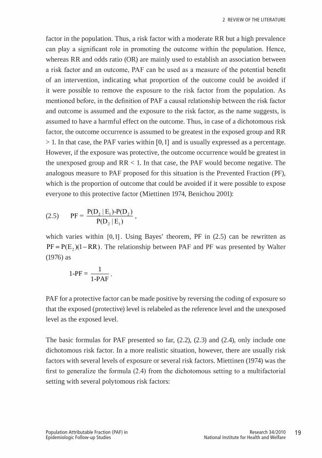
factor in the population. Thus, a risk factor with a moderate RR but a high prevalence can play a significant role in promoting the outcome within the population. Hence, whereas RR and odds ratio (OR) are mainly used to establish an association between a risk factor and an outcome, PAF can be used as a measure of the potential benefit of an intervention, indicating what proportion of the outcome could be avoided if it were possible to remove the exposure to the risk factor from the population. As mentioned before, in the definition of PAF a causal relationship between the risk factor and outcome is assumed and the exposure to the risk factor, as the name suggests, is assumed to have a harmful effect on the outcome. Thus, in case of a dichotomous risk factor, the outcome occurrence is assumed to be greatest in the exposed group and RR > 1. In that case, the PAF varies within [0,1] and is usually expressed as a percentage. However, if the exposure was protective, the outcome occurrence would be greatest in the unexposed group and RR < 1. In that case, the PAF would become negative. The analogous measure to PAF proposed for this situation is the Prevented Fraction (PF), which is the proportion of outcome that could be avoided if it were possible to expose everyone to this protective factor (Miettinen 1974, Benichou 2001):
(2.5) 2 1 2
2 1
P(D | E )-P(D )PF = P(D | E )
,
which varies within [0,1] . Using Bayes’ theorem, PF in (2.5) can be rewritten as
2PF P(E )(1 RR)= − . The relationship between PAF and PF was presented by Walter (1976) as
11-PF =
1-PAF.
PAF for a protective factor can be made positive by reversing the coding of exposure so that the exposed (protective) level is relabeled as the reference level and the unexposed level as the exposed level.
The basic formulas for PAF presented so far, (2.2), (2.3) and (2.4), only include one dichotomous risk factor. In a more realistic situation, however, there are usually risk factors with several levels of exposure or several risk factors. Miettinen (1974) was the first to generalize the formula (2.4) from the dichotomous setting to a multifactorial setting with several polytomous risk factors:
20 Research 34/2010National Institute for Health and Welfare
Population Attributable Fraction (PAF) in Epidemiologic Follow-up Studies
2 REvIEW oF tHE lItERAtuRE
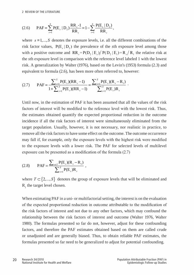
(2.6) 22
1 1
RR -1 P(E | D )PAF P(E | D ) 1RR RR
S Ss s
ss ss s= =
= = −∑ ∑ ,
where 1,...,s S= denotes the exposure levels, i.e. all the different combinations of the risk factor values, 2P(E | D )s the prevalence of the sth exposure level among those with a positive outcome and 2 2 1 1RR =P(D | E ) P(D | E )=R Rs s s the relative risk at the sth exposure level in comparison with the reference level labeled 1 with the lowest risk. A generalization by Walter (1976), based on the Levin’s (1953) formula (2.3) and equivalent to formula (2.6), has been more often referred to, however:
(2.7) 11 1
1 1
P(E )(RR 1) P(E )(R R )PAF
1 P(E )(RR 1) P(E )R
S Ss s s ss s
S Ss s s ss s
= =
= =
− −= =
+ −∑ ∑∑ ∑
.
Until now, in the estimation of PAF it has been assumed that all the values of the risk factors of interest will be modified to the reference level with the lowest risk. Thus, the estimates obtained quantify the expected proportional reduction in the outcome incidence if all the risk factors of interest were simultaneously eliminated from the target population. Usually, however, it is not necessary, nor realistic in practice, to remove all the risk factors to have some effect on the outcome. The outcome occurrence may fall if, for example, only the exposure levels with the highest risk were modified to the exposure levels with a lower risk. The PAF for selected levels of multilevel exposure can be presented as a modification of the formula (2.7)
(2.8) 1
1
P(E )(R R )PAF
P(E )Rs ss T
Ss ss
∈
=
−= ∑
∑,
where { }2,...,T S⊂ denotes the group of exposure levels that will be eliminated and R1 the target level chosen. When estimating PAF in a uni- or multifactorial setting, the interest is on the evaluation of the expected proportional reduction in outcome attributable to the modification of the risk factors of interest and not due to any other factors, which may confound the relationship between the risk factors of interest and outcome (Walter 1976, Walter 1980). The formulas presented so far do not, however, adjust for these confounding factors, and therefore the PAF estimates obtained based on them are called crude or unadjusted and are generally biased. Thus, to obtain reliable PAF estimates, the formulas presented so far need to be generalized to adjust for potential confounding.
21Research 34/2010National Institute for Health and Welfare
Population Attributable Fraction (PAF) in Epidemiologic Follow-up Studies
2 REvIEW oF tHE lItERAtuRE
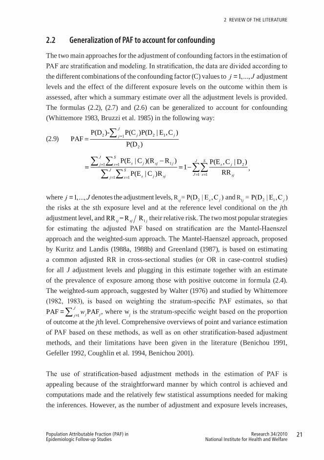
2.2 Generalization of PAF to account for confounding
The two main approaches for the adjustment of confounding factors in the estimation of PAF are stratification and modeling. In stratification, the data are divided according to the different combinations of the confounding factor (C) values to 1,...,j J= adjustment levels and the effect of the different exposure levels on the outcome within them is assessed, after which a summary estimate over all the adjustment levels is provided. The formulas (2.2), (2.7) and (2.6) can be generalized to account for confounding (Whittemore 1983, Bruzzi et al. 1985) in the following way:
(2.9)
2 2 1 1=1 1 1 2
1 12 1 1
P(D )- P(C )P(D | E ,C ) P(E | C )(R R ) P(E ,C | D )PAF 1
P(D ) RRP(E | C )R
J J SJ Sj j s j sj jj j s s j
J SJ s sjs j sjj s
= =
= == =
−= = = −
∑ ∑ ∑ ∑∑∑ ∑
2 2 1 1=1 1 1 2
1 12 1 1
P(D )- P(C )P(D | E ,C ) P(E | C )(R R ) P(E ,C | D )PAF 1
P(D ) RRP(E | C )R
J J SJ Sj j s j sj jj j s s j
J SJ s sjs j sjj s
= =
= == =
−= = = −
∑ ∑ ∑ ∑∑∑ ∑
,
where 1,...,j J= denotes the adjustment levels, Rsj= 2P(D | E ,C )s j and R1j = 2 1P(D | E ,C )j the risks at the sth exposure level and at the reference level conditional on the jth adjustment level, and 1RR = R Rsj sj j their relative risk. The two most popular strategies for estimating the adjusted PAF based on stratification are the Mantel-Haenszel approach and the weighted-sum approach. The Mantel-Haenszel approach, proposed by Kuritz and Landis (1988a, 1988b) and Greenland (1987), is based on estimating a common adjusted RR in cross-sectional studies (or OR in case-control studies) for all J adjustment levels and plugging in this estimate together with an estimate of the prevalence of exposure among those with positive outcome in formula (2.4). The weighted-sum approach, suggested by Walter (1976) and studied by Whittemore (1982, 1983), is based on weighting the stratum-specific PAF estimates, so that
1PAF PAFJ
j jjw
==∑ , where wj is the stratum-specific weight based on the proportion
of outcome at the jth level. Comprehensive overviews of point and variance estimation of PAF based on these methods, as well as on other stratification-based adjustment methods, and their limitations have been given in the literature (Benichou 1991, Gefeller 1992, Coughlin et al. 1994, Benichou 2001).
The use of stratification-based adjustment methods in the estimation of PAF is appealing because of the straightforward manner by which control is achieved and computations made and the relatively few statistical assumptions needed for making the inferences. However, as the number of adjustment and exposure levels increases,

22 Research 34/2010National Institute for Health and Welfare
Population Attributable Fraction (PAF) in Epidemiologic Follow-up Studies
2 REvIEW oF tHE lItERAtuRE
computations become burdensome to perform and obtaining a reasonable number of subjects for all strata difficult to guarantee (Breslow and Day 1980). Furthermore, stratification requires that both the risk factors of interest and the confounding factors be categorical, which may result in loss of information. To avoid these problems, alternative adjustment strategies based on modeling have been developed. In modeling, the relationships between risk factors and the outcome are expressed as a mathematical function, and risk attributable to exposure to a risk factor is represented by the change in risk predicted by the model when the exposure level is changed form one value to another. The use of regression models allows flexible and efficient estimation of the adjusted PAF, as several categorical or continuous risk factors or confounding factors with or without their interactions, allowing also for the analysis of potential effect modification, can be included in the models. Furthermore, regression models yield maximum likelihood estimators that have favorable asymptotic properties. Of course, the correctness of the assumptions inherent in the models chosen need to be tested when applying them to different datasets.
The idea of applying regression models to the estimation of PAF was first suggested by Walter (1976), Sturmans et al. (1977) and Fleiss (1979). Greenland (1987) proposed a modification of the previously mentioned Mantel-Haenszel approach for case-control studies, in which a maximum likelihood estimate of OR from conditional logistic regression was used in the PAF formula (2.4) and provided also the corresponding variance estimate. Bruzzi et al. (1985) were, however, the first to fully exploit the flexibility of the regression models in the estimation of the adjusted PAF from case-control studies. They used the last formulation of the PAF formula (2.9), estimated the prevalences 2= P(E ,C | D )sj s jp from the observed distribution of the cases, and showed how the logistic model could be used to estimate the risk of outcome at different adjustment levels (Rsj ). According to the logistic regression model
(2.10) 2
2
P(D | )log1 P(D | )
TX XX
β=−
,
where 1( ,..., )TmX X X= is the vector of all factors considered relevant (risk factors and confounding factors) and 1( ,..., )Tmβ β β= the regression coefficients corresponding to them. Thus, the risk of a positive outcome is given by
2
exp( )R = P(D | )1 exp( )
T
T
XXX
ββ
=+ .
23Research 34/2010National Institute for Health and Welfare
Population Attributable Fraction (PAF) in Epidemiologic Follow-up Studies
2 REvIEW oF tHE lItERAtuRE
The RR in formula (2.9) can then be replaced by using the OR estimated through logistic regression. Variance estimators for all types of case-control studies were later developed by Benichou and Gail (1990) by applying the delta method (Benichou and Gail 1989). Greenland and Drescher (1993) further generalized the PAF estimator provided by Bruzzi et al. (1985) by using a model-based estimate also for the quantities psj. The model-based approach proposed by Bruzzi et al. (1985) can also be applied to cross-sectional studies; subsequently Basu and Landis (1995) extended the methodology regarding the variance estimation in this design.
Most of the literature on the model-based estimation of PAF has thus focused on case-control and cross-sectional studies, and the point and interval estimation of model-adjusted PAF from these designs has been quite thoroughly discussed and applied in the literature (Benichou 1991, Coughlin et al. 1994, Benichou 2001). The model-adjusted estimation of PAF in cohort studies has been dealt with to a lesser extent, however. An approximative approach for the estimation of PAF in cohort studies, in which only the occurrence of the event of interest by a certain follow-up time is observed (i.e. a binary outcome variable), whereas the timing of the event is ignored, has been proposed in the literature (Deubner et al. 1980, Basu and Landis 1995). In this case, the only difference in comparison to the cross-sectional study is that the outcome is not observed simultaneously with the risk factors but after a fixed follow-up time, and thus the same methods, i.e. the logistic model described in (2.10), as for the estimation of PAF and its confidence interval in cross-sectional studies can be applied. This approach, however, may lose information and produces reliable estimates only in cases in which there is no censoring during follow-up. Later on, the model-based approach for the estimation of PAF proposed by Bruzzi et al. (1985) has also been extended to cohort studies by using the relative risk estimate obtained from Poisson or pooled logistic regression models (Spiegelman et al. 2007).
Thus far, it has been typical not to take into account the time perspective in the estimation of PAF, which results in static PAF estimates. In cohort studies with time-to-event data, dynamic, time-varying PAF estimates are, however, needed. Although attempts to define and calculate dynamic PAFs in cohort studies have been made (Silverberg et al. 2004, Chen et al. 2006, Samuelsen and Eide 2008, Cox et al. 2009), further development is still required.
24 Research 34/2010National Institute for Health and Welfare
Population Attributable Fraction (PAF) in Epidemiologic Follow-up Studies
2 REvIEW oF tHE lItERAtuRE
2.3 Model-based estimation of PAF in a cohort study design
Let T be a non-negative continuous random variable representing the length of follow-up in cohort studies, determined as the time from the baseline to the occurrence of the event of interest or censoring (either due to loss to follow-up, death unrelated to the event of interest (if other than death) or end of follow-up), whichever comes first. We denote the underlying continuous failure time distribution by ( )f t . The cumulative distribution function
0( ) P( ) ( )
tF t T t f u du= ≤ = ∫ then gives the probability that the
event has occurred by time t. The survival function ( ) P( ) 1 ( )S t T t F t= > = − is defined as the probability that the event has not occurred by time t. The probability distribution of T can be specified using the hazard function h( t ). The product ( )h t tΔ approximates the probability of the event occurrence within a short time interval [ , ]t t t+ Δ , conditional upon survival without the event occurrence up to time t. The hazard function h( t ) is defined as
0
P( | ) ( )( ) lim( )t
t T t t T t f th tt S tΔ →
≤ ≤ + Δ >= =Δ
.
In a simple situation, in which the effect of only one dichotomous risk factor, to which all the individuals in the population are either exposed 2(E ) or unexposed 1(E ), on the outcome occurrence is followed, the proportion of outcome by time t can be denoted by 2 2 2 1 2 1( ) P(E )P( | E ) (1 P(E ))P( | E ) ( ) (1 ) ( )F t T t T t pF t p F t= ≤ + − ≤ = + − ,
where 2P(E )p = is the proportion exposed. In survival analysis, however, often the corresponding survival function 2 1( ) ( ) (1 ) ( )S t pS t p S t= + − , indicating the proportion of survival, is used. Similarly, the overall population hazard function is
2 12 1
2 1
( ) (1 ) ( )( ) ( ) ( ) (1 ( )) ( )( ) (1 ) ( )
pf t p f th t p t h t p t h tpS t p S t
+ −= = + −+ − ,
where
2 2
2 1
( ) ( )( )( ) (1 ) ( ) ( )pS t pS tp t
pS t p S t S t= =
+ −
is the proportion exposed at time t.
Two main PAF definitions for cohort studies with censored time-to-event data have been proposed. In the first definition of Population Attributable Hazard Fraction (PAHF), the effect of the hypothetical risk factor modification to the low-risk level is estimated at the instantaneous time point t:
25Research 34/2010National Institute for Health and Welfare
Population Attributable Fraction (PAF) in Epidemiologic Follow-up Studies
2 REvIEW oF tHE lItERAtuRE
(2.11) 1 2 1t
1 2 1
( ) ( ) ( )( ( ) ( )) ( )(HR( ) 1)PAHF( ) ( ) ( )( ( ) ( )) 1 ( )(HR( ) 1)
h t h t p t h t h t p t th t h t p t h t h t p t t− − −= = =
+ − + −,
where 2 1HR( ) ( ) ( )t h t h t= denotes instantaneous hazard ratio at time t (Chen et al. 2006, Samuelsen and Eide 2008). This measure thus describes the approximate proportion of events that could be avoided by the risk factor modification in a short time interval [ , ]t t t+ Δ , where 0tΔ → . Some authors (Silverberg et al. 2004, Samuelsen and Eide 2008) have used the proportion exposed at baseline, (0)p p= , in the calculation of the Population Attributable Hazard Fraction (2.11), instead of the proportion exposed at time t, ( )p t :
(2.12) 1 2 1t
1 2 1
( ) ( ) ( ( ) ( )) (HR( ) 1)PAHF( ) ( ) ( ( ) ( )) 1 (HR( ) 1)
h t h t p h t h t p th t h t p h t h t p t− − −= = =
+ − + −.
This formula corresponds to the traditional PAF formula (2.3), where RR is replaced by HR( )t obtained from survival models. Nonetheless, it is considered to be a naive parameter as it does not consider how the prevalence of exposed individuals changes during the follow-up (Samuelsen and Eide 2008).
The most popular model used to analyze survival data is the proportional hazards model presented by Cox (1972). According to the Cox model, 0( ; ) ( ) exp( )Th t X t Xλ β= , where
0 ( )tλ denotes the baseline hazard, 1( ,..., )TmX X X= the risk factors and 1( ,..., )Tmβ β β=the regression coefficients corresponding to them. In the proportional hazards model, the covariates are thus assumed to affect the hazard function in a multiplicative time-independent way. The Cox model is also the most popular model used for the estimation of PAF in cohort studies. Chen et al. (2006) used the Cox model to obtain an estimate for HR( )t in (2.11) in case of a dichotomous risk factor { }0,1X ∈ :
0
0
( ) exp( )( ; 1)HR( ; ) exp( )( ; 0) ( )
th t Xt Xh t X t
λ β βλ
== = == .
Similarly, the formula (2.11) can be generalized to a multifactorial setting, in the presence of potential confounding, by denoting
*0
* *0
( ) exp( )( ; )HR( ; ) exp(( ) )( ; ) ( ) exp( )
TT T
T
t Xh t Xt X X Xh t X t X
λ β βλ β
= = = − ,
where X is the vector of all factors considered relevant (risk factors and confounding factors), of which only the modifiable risk factors whose effect we wish to measure
26 Research 34/2010National Institute for Health and Welfare
Population Attributable Fraction (PAF) in Epidemiologic Follow-up Studies
2 REvIEW oF tHE lItERAtuRE
in the calculation of PAF will have a different value in X *, while the rest of the factors retain their values (Samuelsen and Eide 2008). The risk factors included in X can be categorical, continuous or their interactions. The semiparametric Cox model thus enables the elimination of the unspecified underlying baseline hazard from the instantaneous hazard ratio HR( ; )t X , making it time-independent. Also, all factors other than the risk factors of interest which are modified are canceled out in the calculation of *exp(( ) )T TX X β− . In case the Cox model were also used to estimate HR( ; )t X in formula (2.12), in which the proportion exposed at baseline is used in the calculation of Population Attributable Hazard Fraction, the entire function would become time-independent.
According to the second definition of PAF for cohort studies with censored time-to-event data, the proportion of events during a follow-up time interval (0, ]t which could be avoided by the risk factor modification is estimated as (Chen et al. 2006, Samuelsen and Eide 2008, Cox et al. 2009):
(2.13) 1 1 1 2(0, ]
1 1 2
( ) ( ) ( ) ( ) ( ( ) ( ))PAF( ) 1 ( ) 1 ( ) ( ( ) ( ))t
F t F t S t S t p S t S tF t S t S t p S t S t
− − −= = =− − + −
.
This formula corresponds to the traditional PAF formula (2.2) when a particular time point is fixed (t = t’), P(D2 ) = F(t’). An alternative measure, Population Attributable Survival Fraction (PASF), in which the proportion of survival due to the hypothetical risk factor modification, 1( ) ( )S t S t− , is calculated, has also been proposed by Cox et al. (2009):
(2.14) 1(0, ]
1
( ) ( )PASF( )t
S t S tS t
−= .
The PASF thus estimates the gain in survival rather than the decrease in risk as (2.13). The formulas (2.13) and (2.14) can be generalized to a multifactorial setting, in the presence of potential confounding, by replacing ( )S t by
0( ; ) exp ( ; )
tS t X h u X du⎡ ⎤= −⎢ ⎥⎣ ⎦∫
and ( )1S t by * *
0( ; ) exp ( ; )
tS t X h u X du⎡ ⎤= −⎢ ⎥⎣ ⎦∫ , where X once again denotes the vector of
all relevant factors, which can be categorical, continuous or their interactions, of which only the modifiable risk factors of interest have a different value in X *.
When the Cox model with the proportional hazards assumption is used in the estimation of PAF, as was done by Chen et al. (2006) and Samuelsen and Eide (2008), the survival function in (2.13) and (2.14) is given by 00
( ) exp ( ) exp( )t TS t u X duλ β⎡ ⎤= −⎢ ⎥⎣ ⎦∫ .
In this case, the unspecified underlying cumulative time-dependent baseline hazard,

27Research 34/2010National Institute for Health and Welfare
Population Attributable Fraction (PAF) in Epidemiologic Follow-up Studies
2 REvIEW oF tHE lItERAtuRE
0 00( ) ( )
tt u duλΛ = ∫ , cannot be eliminated as in formulas (2.11) and (2.12), and
thus to calculate PAF it needs to be estimated. One possibly way of doing this is to use the Breslow estimator (Breslow 1974, Lin 2007) as proposed by Chen et al. (2006) and Samuelsen and Eide (2008). Alternatively, the baseline hazard may be specified parametrically, 0 0( ) ( ; )t tλ λ θ= and ( , )T Tβ θ be estimated by the maximum likelihood method (Samuelsen and Eide 2008). If the proportionality assumption in the Cox proportional hazards model is questionable, a stratified Cox model may be used (Therneau and Grambsch 2000). It allows the form of the underlying hazard function to vary across k levels of the stratification variables which did not satisfy the proportionality assumption: 0( ; ) ( ) exp( )T
kh t X t Xλ β= . Alternative modeling methods, such as parametric accelerated failure time models or additive models, may also be applied (Samuelsen and Eide 2008). Parametric accelerated failure time models assume that covariates act multiplicatively on the predicted event time by some constant, 0 1 1log ... m mT X Xβ β β σε= + + + + , where 0β and σ are the intercept and scale parameters and ε the random disturbance term (Kay and Kinnersley 2002), whereas additive models assume that covariates, which are allowed to be time-varying, act in an additive manner on an unknown baseline hazard,
0 1 1( ; ) ( ) ( ) ( ) ... ( ) ( )m mh t X t X t t X t tλ β β= + + + , and may be fitted by non-parametric, semiparametric or parametric methods (Aalen 1989, Lim and Zhang 2009).
Usually, it is more useful to demonstrate the effect of the risk factor modification during a certain time interval, instead of at some particular time point t, as is done in (2.11) and (2.12). For example, in case of an event that is inevitable, such as death, the event can only be delayed and, thus, it is useful to calculate PAF estimates during time intervals of different lengths in order to demonstrate the effect of the risk factor modification in different time scenarios. Furthermore, due to the inevitability of death, the PAF will eventually approach zero as time goes to infinity and thus become meaningless, further emphasizing the importance of specifying a certain time interval. Comparison of the PAF estimates calculated in cohort studies with different lengths of follow-up is also questionable for these same reasons.
So far, point estimation of the dynamic PAF based on different definitions, (2.11), (2.12), (2.13), and (2.14), has been presented. There are also different approaches to estimating the variance of the PAF estimates: analytical variance estimation or resampling-based methods, such as bootstrap. Variance estimation of point estimates of PAF obtained using (2.12) and (2.13), based on the Cox model with the Breslow
28 Research 34/2010National Institute for Health and Welfare
Population Attributable Fraction (PAF) in Epidemiologic Follow-up Studies
2 REvIEW oF tHE lItERAtuRE
estimator for the cumulative baseline hazard using non-parametric bootstrapping, was carried out by Samuelsen and Eide (2008), which also enabled a comparison of the results. Resampling-based variance estimation is, however, more computer intensive than analytical variance estimation. Asymptotic variance estimation for (2.13), based on the Cox model with the Breslow estimator for the cumulative baseline hazard, was demonstrated by Chen et al. (2006). Although asymptotic variance estimation applying the delta method for fully parametrized models has been suggested, it has not yet been demonstrated in the literature. Various methods for the calculation of confidence intervals for PAF can also be applied once the point and variances estimates of PAF have been obtained. The regular confidence interval based on PAF and its estimated standard error is based on the asymptotic normality of PAF. This normal approximation is not accurate when the sample size is small and, thus, to improve the normal approximation confidence intervals based on complementary log-transformed, log(1 PAF)− , (Walter 1975) and logit-transformed, log (PAF (1 PAF))− , (Leung and Kupper 1981) PAF estimates have been proposed and compared (Whittemore 1982). The complementary logarithmic transformation guarantees that the retransformed PAF estimates remain in their natural range from −∞ to 1, whereas logit-transformation forces the estimates within (0, 1) (Greenland and Drescher 1993).
When estimating PAF from cohort studies with time-to-event data, censoring is involved and needs to be considered in the estimation of PAF. There may also be censoring from different sources depending on the event of interest (Andersen et al. 1993, Rothman et al. 2008, Gail and Pfeiffer 2005, Schumacher et al. 2007, Samuelsen and Eide 2008). If the event of interest is inevitable, such as death from all causes, i.e. total mortality, censoring due to end of follow-up or loss to follow-up needs to be considered. If the event of interest is, however, not inevitable, such as disease incidence, also censoring due to competing risks, events that compete with the event of interest to remove persons from the population at risk, such as death due to reasons other than the event of interest, may occur before occurrence of the event of interest and needs to be considered. Note that although both loss to follow-up and loss to competing risks are here treated as two forms of censoring, they are very different phenomena (Rothman et al. 2008). After censoring due to loss to follow-up the outcome may still occur, whereas censoring due to competing risks such as death inhibits the outcome from occurring. Furthermore, losses to follow-up are not usually expected to be related to the risk factors of interest, whereas losses to competing risks may be. If for example the risk factors that are related to the incidence of the disease are also related to mortality, the modification of these risk factors is likely to affect the risk of the disease and the
29Research 34/2010National Institute for Health and Welfare
Population Attributable Fraction (PAF) in Epidemiologic Follow-up Studies
2 REvIEW oF tHE lItERAtuRE
risk of death, differently depending on the direction and magnitude of the relationship between the risk factors and the outcome. Thus, in the estimation of PAF for disease incidence, in addition to the censoring due to follow-up, censoring due to death needs to be taken into account as well. Ignoring censoring due to death when estimating PAF for disease incidence means that the estimates obtained only apply under the assumption that no one dies during the follow-up during which the incidence of disease is estimated. Thus, we need different estimators of PAF depending on the event of interest in order to obtain accurate results. Samuelsen and Eide (2008) have discussed this issue with respect to the context of a specific study, but as far as I know PAF formulas have not been generalized to account for censoring due to competing risks.
The pooling of cohort studies using meta-analysis techniques is becoming increasingly popular, as it increases the power to detect the associations between risk factors and the outcome. Thus, pooling becomes especially useful when the estimation of the strength of association is carried out in smaller subpopulations: for example, in categories of potential effect modifying factors. Although methodology for the pooling of relative risks has been applied in many studies (for example in Knekt et al. 2004 and Smith-Warner et al. 2006), as far as the author of this dissertation knows this methodology has not yet been generalized to pooling of the PAF estimates. Neither has the analysis of the impact of potential effect modification in the calculation of the dynamic PAF yet been considered.
Finally, although the estimation of PAF has been increasingly dealt with in methodological research since its introduction in 1953 (Levin 1953), relatively few publicly available programs implementing the developed estimation methods have been presented. Before the 1990s, there seemed to be no publicly available programs for estimating PAF from any study designs. Since then, programs for estimating PAF from case-control and cross-sectional studies in different programming languages (SAS, Stata, R/S+) have become available (Mezzetti et al. 1996, Brady 1998, Kahn et al. 1998, Grömping and Weimann 2004, Eide 2006, Lehnert-Batar 2006, Rückinger et al. 2009, Rämsch et al. 2009). However, as far as the author of this dissertation knows only one publicly available program for the estimation of static PAF in cohort studies has been provided (Spiegelman et al. 2007). Thus, it seems that no publicly available programs for estimating dynamic PAF during a certain time interval (0, ]t (2.13) yet exist. To promote the estimation of PAF for follow-ups of different lengths in both single and pooled cohort studies, a publicly available and flexible program, which takes into account censoring from different sources, is urgently needed.
30 Research 34/2010National Institute for Health and Welfare
Population Attributable Fraction (PAF) in Epidemiologic Follow-up Studies
3 AIMS oF THE STUDY
The main objective of this study was to derive formulas for the calculation of Population Attributable Fraction (PAF) and its variance both for total mortality and disease incidence in a cohort study design. These formulas cover both the main effects and interactions. Also, pooling of the PAF estimates and their variances from several single cohorts was demonstrated. In addition, a program consisting of SAS macros based on these formulas was developed. Finally, the application of these new formulas and the program was illustrated in a data example on risk factors of type 2 diabetes.
The specific aims of the study were:
1. to derive formulas for the estimation of PAF and its variance for total mortality in a cohort study design using a piecewise constant hazards model (Original publication I);
2. to derive formulas for the estimation of PAF and its variance for disease incidence in a cohort study design using a piecewise constant hazards model and taking into account censoring due to death (Original publication II);
3. to develop a program based on SAS macros for the calculation of PAF both for total mortality and disease incidence in a cohort study design using a piecewise constant hazards model (Original publication III); and
4. to apply the new formulas and program for the estimation of PAF for disease incidence to evaluate the relative importance of modifiable potential risk factors of type 2 diabetes as well as their potential effect modifying factors in a pooled cohort study design consisting of two representative Finnish cohorts (Original publication IV).
31Research 34/2010National Institute for Health and Welfare
Population Attributable Fraction (PAF) in Epidemiologic Follow-up Studies
4 STATISTICAL METHoD FoR THE ESTIMATIon oF PAF In A CoHoRT STUDY DESIGn
4.1 Definition of PAF in a cohort study design
4.1.1 General definition of PAF
Suppose that at baseline (t = 0) the study population consists of n individuals who are free of the outcome of interest (A). Each individual’s m risk factor values 1( ,..., )Ti i imX X X= , where i = 1,...,n , are known. The risk factors measured at baseline are assumed to be fixed and causally related to the outcome. The study population is subsequently followed for a given period of time, with the length of follow-up for each individual ( Ti ) determined as the time from baseline to the date of the outcome of interest or censoring, whichever comes first. Population Attributable Fraction (PAF) assesses the proportion of the outcome occurrence that could be avoided during a follow-up time interval (0, t] if it was possible to change some risk factor values to their chosen target values, 1( ,..., )Ti i imX X X= → * * *
1( ,..., )Ti i imX X X= . In this notation, iX is the vector of all risk factors and confounding factors of the ith individual, and thus only the modifiable risk factors whose effect we are interested in measuring may have a different value in
*iX while the rest of the factors retain their values. The PAF is thus defined as
(4.1) * *
1 1 1
1 1
{ | } { | } { | }PAF( ) 1
{ | } { | }
n n ni i i i i ii i i
n ni i i ii i
A X A X A XA
A X A X= = =
= =
Ρ − Ρ Ρ= = −
Ρ Ρ∑ ∑ ∑
∑ ∑,
where { | }i iA XΡ is the model-based probability of the outcome occurrence during the risk period (0, t] for the ith individual given the risk factors iX .
4.1.2 Definition of PAF for total mortality
If the outcome of interest is death, PAF is defined as the proportion of mortality that could theoretically be delayed during a follow-up time interval (0, t] if its risk factors were modified. Let MT denote the time of death. Then the expected excess mortality during follow-up time t due to certain modifiable risk factors in iX is given by (4.1) as
(4.2) PAF( )MT t≤ = *
1
1
{ | }1
{ | }
n Mi ii
n Mi ii
T t X
T t X=
=
Ρ ≤−
Ρ ≤∑∑
.
32 Research 34/2010National Institute for Health and Welfare
Population Attributable Fraction (PAF) in Epidemiologic Follow-up Studies
4 StAtIStIcAl MEtHod FoR tHE EStIMAtIoN oF PAF IN A coHoRt StudY dESIGN
The expected excess mortality at any chosen interval ( , ]t t t+ Δ can be calculated similarly by using the probabilities { | }M
i iP t T t t X< ≤ + Δ .
4.1.3 Definition of PAF for disease incidence
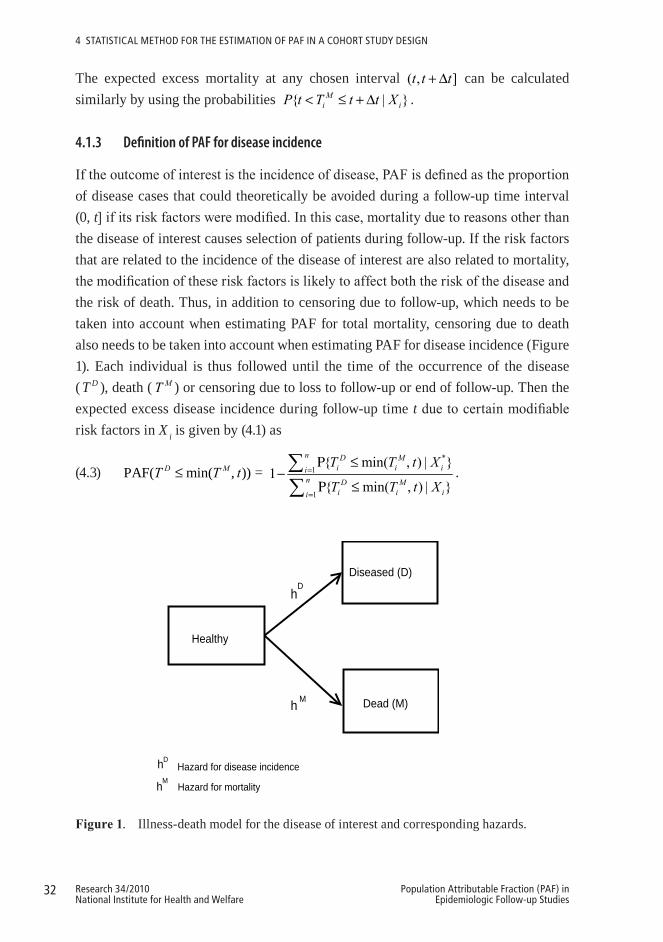
If the outcome of interest is the incidence of disease, PAF is defined as the proportion of disease cases that could theoretically be avoided during a follow-up time interval (0, t] if its risk factors were modified. In this case, mortality due to reasons other than the disease of interest causes selection of patients during follow-up. If the risk factors that are related to the incidence of the disease of interest are also related to mortality, the modification of these risk factors is likely to affect both the risk of the disease and the risk of death. Thus, in addition to censoring due to follow-up, which needs to be taken into account when estimating PAF for total mortality, censoring due to death also needs to be taken into account when estimating PAF for disease incidence (Figure 1). Each individual is thus followed until the time of the occurrence of the disease ( T D ), death ( MT ) or censoring due to loss to follow-up or end of follow-up. Then the expected excess disease incidence during follow-up time t due to certain modifiable risk factors in X i is given by (4.1) as
(4.3) PAF( min( , ))D MT T t≤ = *
1
1
{ min( , ) | }1
{ min( , ) | }
n D Mi i ii
n D Mi i ii
T T t X
T T t X=
=
Ρ ≤−
Ρ ≤∑∑
.
Diseased (D)
Dead (M)
hD
h M
Healthy
hD Hazard for disease incidence
hMHazard for mortality
1
Figure1. Illness-death model for the disease of interest and corresponding hazards.

33Research 34/2010National Institute for Health and Welfare
Population Attributable Fraction (PAF) in Epidemiologic Follow-up Studies
4 StAtIStIcAl MEtHod FoR tHE EStIMAtIoN oF PAF IN A coHoRt StudY dESIGN
It is not, however, self-evident that if certain risk factor values, related both to the occurrence of the disease and death, were modified, the probability of the disease occurrence during follow-up would decrease. Although it is probable that the person would contract the disease later, he or she would probably also live longer, and thus still contract the disease before dying. The PAF could thus turn out to be negative. One way of reducing the likelihood of this would be to estimate the excess disease incidence up to a certain age.
4.2 General model assumptions
The following assumptions in the calculation of PAF for total mortality or for disease incidence from the cohort study design are made in this study. Proportional hazards models are applied. The hazard of death is ( )Mh t and the hazard of disease incidence ( )Dh t . The corresponding cumulative hazard functions are then ( )MH t =
0( )
t Mh u du∫ and ( )DH t = 0
( )t Dh u du∫ . We will also define short-hand notations ( )MS t
= exp ( )MH t⎡ ⎤−⎣ ⎦ and ( )DS t = exp ( )DH t⎡ ⎤−⎣ ⎦ , which will not, however, have survival function interpretations in the situation with competing risks. For each individual, the hazard functions are assumed to depend on the X vector of observed risk factors:
( ; )Mh t X and ( ; )Dh t X . The time of death T M and the time of the occurrence of the disease T D are assumed to be conditionally independent given X, which is assumed to include all relevant risk factors for both mortality and disease incidence. The hazard function corresponding to disease-free survival, min(T M ,T D), is thus assumed to be
( ; ) ( ; )D Mh t X h t X+ . Then, the probability that the first event occurring at a given time point t is the disease is
{ } ( ; )min( , ) min( , )
( ; ) ( ; )
DM D D M D
D M
h t XT T T T T th t X h t X
Ρ = = =+
.
There may still be right-censoring by T C, which is assumed to be conditionally independent of T M and T D given X. If the outcome of interest is death, we then observe for each individual T C = min(T C, T M) in case of right-censoring or T M = min(T C, T M) in case of death. If the outcome of interest is incidence of disease, we observe T C = min(T C,
T M, T D), T M = min(T C, T M, T D), T D < T C = min(T C, T M) or T D < T M = min(T C < T M ). It is important to note, that the definition of PAF does not depend on T C.

34 Research 34/2010National Institute for Health and Welfare
Population Attributable Fraction (PAF) in Epidemiologic Follow-up Studies
4 StAtIStIcAl MEtHod FoR tHE EStIMAtIoN oF PAF IN A coHoRt StudY dESIGN
4.2.1 Piecewise constant hazards model
In the calculation of PAF, the waiting times T M and T D are assumed to be independent and to follow a proportional hazards model with piecewise constant baseline hazard functions, given X. In a parametric piecewise constant hazards model, the follow-up time is partitioned into J-1 intervals 1 2 2 3 1 1(0 , ], ( , ], , ( , ], , ( , ]j j J Ja a a a a a a a− −= … … , where 1j ja a− < for all j and the hazard for the ith individual
(4.4) ( ; )ih t X =
11{ }0
1
exp( ) j jJ
a t aTi j
j
X β λ − < ≤
=∏
is allowed to depend on time by letting the value of the baseline hazard 0 jλ change at times a j (Friedman 1982). A log-linear function between the risk factors and the hazard function is thus assumed. The effect of age can be taken into account by dividing the range of individual dates of birth into B-1 birth cohorts 1 2 1 1( , ],..., ( , ],..., ( , ]b b B Bv v v v v v− − and then further stratifying the baseline hazard by them ( 0 ijb
λ ) (Korn et al. 1997) . Let us thus denote the hazard of death at time t for the ith individual given the birth cohort bi and risk factors iX = 1( ,..., )Ti imX X as in (4.4)
(4.5) ( ; , )Mi ih t b X =
11{ }
1
( ) j jJ
a t aMij
j
λ − < ≤
=∏ ,
the hazard of disease incidence as
(4.6) ( ; , )Di ih t b X = 11{ }
1
( ) j jJ
a t aDij
j
λ − < ≤
=∏ ,
where
(4.7) 0 exp( ) exp( ) exp( )i i
M M T M M T M Mij jb i jb i ijX X Zλ λ β α β γ= = + =
and
(4.8) 0 exp( ) exp( ) exp( )i i
D D T D D T D Dij jb i jb i ijX X Zλ λ β α β γ= = + = .
In this notation, 0logi i
M Mjb jbα λ= is the logarithm of the baseline hazard of death 0( )
i
Mjbλ
and 0logi i
D Djb jbα λ= the logarithm of the baseline hazard of disease incidence 0( )
i
Djbλ .
Virtually any baseline hazard can be well approximated by choosing closely-spaced cut-points for the intervals. Similarly, Mβ and Dβ are the vectors of regression coefficients

35Research 34/2010National Institute for Health and Welfare
Population Attributable Fraction (PAF) in Epidemiologic Follow-up Studies
4 StAtIStIcAl MEtHod FoR tHE EStIMAtIoN oF PAF IN A coHoRt StudY dESIGN
for death and disease incidence, respectively, for the covariates Xi , which can be either categorical, continuous or their interactions. Furthermore, Zij is the vector with length JB+m, including JB indicators of time interval and birth cohort and the covariates
iX corresponding to the regression coefficients 11 1( , ..., , , ..., )M M M M M TJB mγ α α β β= and
11 1( , ..., , , ..., )D D D D D TJB mγ α α β β= . The *M
ijλ and *Dijλ follow similarly by replacing iX by
*iX in (4.7) and (4.8).
4.3 Model-based calculation of PAF in a cohort study design
4.3.1 Calculation of PAF for total mortality
The probability of death during follow-up time interval (0, t] for the ith individual, given the birth cohort bi and the risk factors Xi , in (4.2) is calculated as
{ | , }Mi i iT t b XΡ ≤ = 1 ( ; , )M
i iS t b X− ,
where the survival function using (4.5) is given by
1
( ; , ) exp ( )J
M Mi i ij j
jS t b X tλ δ
=
⎡ ⎤−⎢ ⎥⎣ ⎦∑ = ,
where ( )j tδ defines the length of follow-up time in the jth interval
(4.9) 1
1 1
1
0 ,( ) ,
,
j
j j j j
j j j
t at t a a t a
a a t aδ
−
− −
−
⎧ ≤⎪= − < ≤⎨⎪ − >⎩
.
The PAF for total mortality during the follow-up time interval (0, t] can then be calculated as in (4.2)
(4.10) { }{ }
*1 1
(0, ]
1 1
1 exp ( )PAF( ) PAF 1
1 exp ( )
n J Mij ji jM M
t n J Mij ji j
tT t
t
λ δ
λ δ
= =
= =
⎡ ⎤− −⎣ ⎦≤ = = −⎡ ⎤− −⎣ ⎦
∑ ∑∑ ∑
,
where Mijλ is given by (4.7) and *M
ijλ follows similarly by replacing iX by *iX in these
formulas.
36 Research 34/2010National Institute for Health and Welfare
Population Attributable Fraction (PAF) in Epidemiologic Follow-up Studies
4 StAtIStIcAl MEtHod FoR tHE EStIMAtIoN oF PAF IN A coHoRt StudY dESIGN
4.3.2 Calculation of PAF for disease incidence
The crude probability of disease occurrence is defined as the probability that an individual who is free of a disease at a specific time, 1ja − , will develop that disease in a subsequent time interval, 1( , ]j ja a− (Gail and Pfeiffer 2005). This probability is, however, affected by mortality due to other causes. Thus, in order to calculate PAF for the incidence of disease (4.3), we need to estimate the probability of disease occurrence when the time of death is also taken into account. The probability of occurrence of a certain disease, given the birth cohort bi and the risk factors Xi in (4.3), using (4.6) is then
{ min( , ) | , }D Mi i i iT T t b XΡ ≤ = 1 11
{ , , } { , }J Di j j i i j j i ij
T T a T a b X a T a b X− −=Ρ = < ≤ Ρ < ≤∑
= , 11( )
DJ ij
i j ijD Mjij ij
S Sλ
λ λ −=−
+∑ ,
where t is chosen to be aj , min( , )D MT T T= and
11exp ( )( )jD M D M
ij ij ij ik ik k kkS S S a aλ λ −=
⎡ ⎤= = − + −⎣ ⎦∑
is the disease-free survival up to time aj. Thus, according to (4.3) the PAF for the incidence of disease is given by
(4.11) PAF( min( , ))D MT T t≤ =
** *, 1* *1 1
, 11 1
( )1
( )
Dn J ij
i j ijD Mi jij ij
Dn J ij
i j ijD Mi jij ij
S S
S S
λλ λ
λλ λ
−= =
−= =
−+
−−
+
∑ ∑
∑ ∑,
where Mijλ is given by (4.7) and D
ijλ by (4.8) and *Mijλ and *D
ijλ follow similarly by replacing iX by *
iX in these formulas.
4.4 Estimation of PAF in a cohort study design
4.4.1 Estimation of PAF for total mortality
EstimationofparametersFor estimating the PAF for total mortality (4.10), we first need to estimate the parameters

37Research 34/2010National Institute for Health and Welfare
Population Attributable Fraction (PAF) in Epidemiologic Follow-up Studies
4 StAtIStIcAl MEtHod FoR tHE EStIMAtIoN oF PAF IN A coHoRt StudY dESIGN
11 1( ,..., , ,..., )M M M M M TJB mγ α α β β= . Note that in some applications the parameters might
be estimated in one population and the PAF be calculated in another (standard) population. The maximum likelihood estimates of Mγ can be obtained by maximizing the overall likelihood function given by
( )ML γ =1 1
( ) exp ( )Mij
n JdM M
ij ij j ii j
tλ λ δ= =
⎡ ⎤−⎣ ⎦∏∏
= { }
1 1
exp( ) exp exp( ) ( )n J
M M Mij ij ij j i
i j
d Z Z tγ γ δ= =
⎡ ⎤−⎣ ⎦∏∏
=
1 1 1 1exp exp exp( ) ( )
n J n JM M Mij ij ij j i
i j i jd Z Z tγ γ δ
= = = =
⎡ ⎤⎛ ⎞ ⎡ ⎤−⎢ ⎥⎜ ⎟ ⎢ ⎥
⎢ ⎥⎝ ⎠ ⎣ ⎦⎣ ⎦∑∑ ∑∑
or the logarithm of the likelihood function given by
1 1 1 1( ) log ( ) exp( ) ( )
n J n JM M M M M
ij ij ij j ii j i j
l L d Z Z tγ γ γ γ δ= = = =
⎛ ⎞= = −⎜ ⎟
⎝ ⎠∑∑ ∑∑ .
In this notation, Mijd is the indicator which indicates at which interval j the event takes
place and thus obtains a value of 1 at that interval; otherwise its value is 0:
(4.12) Mijd = 11, 0 ( ) min( , )
,0, otherwise
j i i j jt t a aδ −< < −⎧⎨⎩
where ( )j tδ defines the length of follow-up time in the jth interval (4.9). The log-likelihood function will be maximized where the score function ( )MS γ , which is a (JB+m) × 1 vector of the first order partial derivatives of the log-likelihood function with respect to each of the JB+m individual elements of Mγ , equals zero:
1 1 1 1
( )( ) exp( ) ( ) 0M n J n J
M M Mij ij ij ij j iM
i j i j
lS d Z Z Z tγγ γ δγ = = = =
∂= = − =∂ ∑∑ ∑∑ .
The asymptotic variance for the estimates ˆMγ can be obtained using the inverse of the Fisher information matrix ( )I γ , which can be obtained as minus of the expected value of the Hessian matrix, which is a (JB+m) × (JB+m) matrix of the second order partial derivatives of the log-likelihood function with respect to all possible combinations of the JB+m individual elements of Mγ :
38 Research 34/2010National Institute for Health and Welfare
Population Attributable Fraction (PAF) in Epidemiologic Follow-up Studies
4 StAtIStIcAl MEtHod FoR tHE EStIMAtIoN oF PAF IN A coHoRt StudY dESIGN
2
1 1
( )( ) exp( ) ( )( )
M n JM M T
ij ij ij j iM M Ti j
lH Z Z Z tγγ γ δγ γ = =
∂= = −∂ ∂ ∑∑ .
Since the score function cannot, however, be solved in closed form, maximum likelihood estimation with iterative methods, such as Newton-Raphson or Fisher Scoring, are required to obtain the parameter estimates 11 1̂
ˆˆ ˆ ˆ( ,..., , ,..., )M M M M M TJB mγ α α β β=
and their estimated covariance matrix M
∑ (Bickel and Doksum 2001). The SAS procedure LIFEREG was used for this purpose (SAS Institute Inc. 2007).
EstimationofPAFIn this section, the PAF for total mortality, (0, ]PAFM
t , is written in brief as PAF. The point estimate of PAF can be obtained by replacing the unknown parameter values Mγ in (4.10) by their point estimates ˆMγ . The variance estimate of PAF can be obtained using the delta method, according to which
(4.13) 2PAF(PAF PAF) (0, )Dn N σ− ⎯⎯→ ,
where the limiting variance of PAF can be consistently estimated by
(4.14) 2PAFσ̂ = PAF PAF
ˆ
TM
M MM M γ γγ γ⎛ ⎞ ⎛ ⎞∂ ∂
∑⎜ ⎟ ⎜ ⎟ =∂ ∂⎝ ⎠ ⎝ ⎠.
The approximate 95% confidence interval of PAF is then obtained by
(4.15) PAF +1.96 2PAFσ̂× .
This normal approximation for the sampling distribution of PAF is not accurate when the sample size is small and the distribution of PAF is skewed, especially when it is skewed towards high values for PAF. In that case, some symmetrizing monotone strictly increasing transformation of PAF, g(PAF), such as the complementary logarithmic transformation, g(PAF) = log(1–PAF), should be used. Then, the PAF in formulas (4.13), (4.14) and (4.15) is replaced by g(PAF) and, finally, the 95% confidence interval of (PAF)g is transformed back to the original scale by using the inverse of the complementary logarithmic transformation given by
(4.16) 1 2(PAF)ˆ(PAF) 1.96 gg g σ− ⎡ ⎤± ×⎣ ⎦ .

39Research 34/2010National Institute for Health and Welfare
Population Attributable Fraction (PAF) in Epidemiologic Follow-up Studies
4 StAtIStIcAl MEtHod FoR tHE EStIMAtIoN oF PAF IN A coHoRt StudY dESIGN
4.4.2 Estimation of PAF for disease incidence
EstimationofparametersFor estimating PAF for incidence of disease (4.11), we first need to estimate the parameters Dγ for disease incidence and Mγ for death. Estimation of the parameters Dγ and Mγ is based on the data of the individual follow-up times until the occurrence of
the disease of interest, death or censoring, whichever comes first: Ti = min( , , )D M Ci i iT T T .
As the right-censoring is assumed to be independent and noninformative (Andersen et al. 1993), we have two events of interest here for which we define corresponding indicator variables for each individual i and interval 1( , ]j ja a− : disease incidence ( D
ijd ) and death ( M
ijd ). The indicator ijd indicates at which interval j the event takes place and thus obtains a value of 1 at that interval; otherwise its value is 0 (4.12).
The overall likelihood function can thus be expressed as:
( , )D ML γ γ = 1 1
( ) ( ) exp ( ) ( )M Dij ij
n Jd dM D D M
ij ij ij ij j ii j
tλ λ λ λ δ= =
⎡ ⎤− +⎣ ⎦∏∏ ,
where min( , )D Mi i it t t= is the event time of the first event and
( )j tδ = 1max(min( , ) ,0)j jt a a −− , as given in equation (4.9), denotes the length of follow-up time at each interval until the time of the event. The overall likelihood function can be rewritten so that the parts related to disease incidence and death are grouped together so that
( , )D ML γ γ = ( ) ( )D ML Lγ γ ,
where
( )DL γ = 1 1
( ) exp ( )Dij
n JdD D
ij ij j ii j
tλ λ δ= =
⎡ ⎤−⎣ ⎦∏∏and
( )ML γ = 1 1
( ) exp ( )Mij
n JdM M
ij ij j ii j
tλ λ δ= =
⎡ ⎤−⎣ ⎦∏∏ .
The log-likelihood function is the sum of the separate log-likelihood functions for Dγ and Mγ . The maximization can thus be made separately for each parameter vector using standard likelihood theory for a piecewise constant hazards model. As both likelihood functions are based on independent observations from exponential distributions, the two sets of maximum likelihood estimates ˆDγ and ˆMγ are known to be asymptotically
40 Research 34/2010National Institute for Health and Welfare
Population Attributable Fraction (PAF) in Epidemiologic Follow-up Studies
4 StAtIStIcAl MEtHod FoR tHE EStIMAtIoN oF PAF IN A coHoRt StudY dESIGN
multivariate normal. They are also asymptotically independent (the Fisher information matrix is block-diagonal). In this study, the SAS procedure LIFEREG was used to compute the estimates ˆDγ and ˆMγ and their estimated covariance matrices ˆ D∑ and ˆ M∑ (SAS Institute Inc. 2007). The approximate sampling distribution of
ˆˆ
D D
M Mnγ γγ γ⎛ ⎞−⎜ ⎟−⎝ ⎠
is then 0 0,
0 0
D
MN⎛ ⎞⎛ ⎞∑⎛ ⎞⎜ ⎟⎜ ⎟⎜ ⎟⎜ ⎟⎜ ⎟⎝ ⎠ ∑⎝ ⎠⎝ ⎠
.
EstimationofPAF In this section, the PAF for disease incidence, (0, ]PAFD
t , is written in brief as PAF. The point estimate of PAF for the incidence of disease is obtained by replacing the unknown parameter values Dγ and Mγ in (4.11) by their point estimates ˆDγ and ˆMγ . A symmetrizing complementary logarithmic transformation of PAF, g(PAF) = log(1–PAF) is used to estimate the confidence interval of PAF . The variance estimate of g(PAF) can be obtained using the delta method (4.13), where the limiting variance of PAF for the incidence of disease can be consistently estimated by
(4.17) 2PAFσ̂ =
PAF PAFˆ
TD
D DD D γ γγ γ⎛ ⎞ ⎛ ⎞∂ ∂
∑⎜ ⎟ ⎜ ⎟ =∂ ∂⎝ ⎠ ⎝ ⎠ +
1 1
PAF PAFˆ
TM
M MM M γ γγ γ⎛ ⎞ ⎛ ⎞∂ ∂
∑⎜ ⎟ ⎜ ⎟ =∂ ∂⎝ ⎠ ⎝ ⎠.
The approximate 95% confidence interval of (PAF)g is then obtained using (4.15) and is finally transformed back to the original scale using (4.16).
4.5 Estimation of PAF in a cohort study design in the presence of potential effect modification
In the calculation of PAF, we may want to consider the potential effect modification, i.e. whether the relationship between the risk factor and the outcome of interest, and thus potentially also PAF, varies according to the values of a potential effect modifying factor. To analyze the impact of the potential effect modifying factor, an interaction term between the risk factor and the potential effect modifying factor is included in the model, which gives separate parameter estimates for the risk factor in the different
41Research 34/2010National Institute for Health and Welfare
Population Attributable Fraction (PAF) in Epidemiologic Follow-up Studies
4 StAtIStIcAl MEtHod FoR tHE EStIMAtIoN oF PAF IN A coHoRt StudY dESIGN
categories of the potential effect modifying factor. Separate PAF estimates are then calculated in the subpopulations defined by the categories of the potential effect modifying factor. The statistical significance of effect modification can be assessed by calculating the confidence intervals for the differences between these PAF estimates. In case of an effect modifying factor with two categories, for example, we estimate the PAF difference 1 2PAF PAF− and its 95% confidence interval
(4.18) 1 2(PAF PAF )− + 1.961 2
2PAF PAFσ̂ −× ,
where PAF is used to denote either PAF for mortality (4.10) or PAF for disease incidence (4.11). The variance of the PAF difference is obtained using the delta method (4.13), where PAF is replaced by 1 2PAF PAF− , and where the limiting variance of
1 2PAF PAF− , 1 2
2PAF PAFσ̂ − , can be consistently estimated using (4.14) in case of total
mortality and using (4.17) in case of incidence of disease.
It is important to note that since both the prevalence of the risk factors and the strength of the association between the risk factors and the outcome affect PAF, the effect modification may be due to either of these components.
4.6 Estimation of PAF in a pooled cohort study design
In a pooled cohort study design, the results from several single cohort studies are summarized using a specific methodology (Knekt et al. 2004, Smith-Warner et al. 2006). To estimate PAF in a pooled cohort study design, the study-specific PAFs are combined, weighting them by the inverse of their variance, in a random-effects model (DerSimonian and Laird 1986):
(4.19) 1
PAF PAFS
ss
sw=
=∑ ,
where
(4.20) 2 1PAF
2 1PAF1
ˆ( )
ˆ( )s
s
s S
s
wσ
σ
−
−=
=∑
,
where PAF s denotes the PAF estimate either for mortality (4.10) or for disease incidence (4.11) from the sth study, ws the weight of the sth study and 2
PAFˆs
σ the variance of the PAF s , where s = 1,…, S is the study number. The statistical significance of the
42 Research 34/2010National Institute for Health and Welfare
Population Attributable Fraction (PAF) in Epidemiologic Follow-up Studies
4 StAtIStIcAl MEtHod FoR tHE EStIMAtIoN oF PAF IN A coHoRt StudY dESIGN
heterogeneity between the study-specific PAFs can be tested by applying the asymptotic DerSimonian and Laird Q statistic (DerSimonian and Laird 1986), thus given by
(4.21) * 2
1(PAF PAF)
S
ss
sQ w=
= −∑ ,
where * 2 1PAFˆ( )
ssw σ −= . The Q test statistic follows under the null hypothesis of a homogeneous PAF an approximate 2
1sχ − distribution. The potential heterogeneity due to potential effect modifying factors can be tested using the Wald test (Stram 1996). Similarly, if the complementary logarithmic transformation of PAF,
(PAF) log(1 PAF)g = − , is used, the PAF in formulas (4.19), (4.20), and (4.21) is replaced by g(PAF). Finally, the pooled point estimate (PAF)g and its confidence interval are transformed back to the original scale by using the inverse of the complementary logarithmic transformation, as in (4.16). Before pooling of estimates from individual studies it is important to determine whether all these studies can be combined for a single effect estimate representative of the phenomenon we are interested to study. To do this, the comparability of the studies with respect to their design, representativeness, distribution of background variables and risk factors, exposure assessment, adjustment for confounding factors, and quality and nature of statistical methods used should be explored and sufficient similarity ascertained. This is usually done to the extent possible through a priori specified inclusion criteria for acceptable studies and through standardisation of all relevant variables between the individual studies and use of the same statistical methods in them whenever possible. Furthermore, when pooling the estimates of the selected studies, homogeneity among them should be tested. If the hypothesis of homogeneity is rejected, the average estimate is unrepresentative, and thus the sources of observed heterogeneity should be explored and the analyses and reporting limited to homogeneous subgroups. In the pooling of PAF estimates in particular, it should be noted that both the strength of the association between the risk factor and the outcome and the prevalence of the risk factor in different studies may influence the heterogeneity.
43Research 34/2010National Institute for Health and Welfare
Population Attributable Fraction (PAF) in Epidemiologic Follow-up Studies
5 SAS PRoGRAM FoR THE ESTIMATIon oF PAF In A CoHoRT STUDY DESIGn
5.1 Background and objectives
As summarized in the review of the literature in Chapter 2, there are no publicly available programs for estimating the dynamic PAF in cohort studies during a certain time interval (0, t]. In this chapter, a program, consisting of separate SAS macros, for the estimation of PAF during a time interval (0, t] and its asymptotic variance both for total mortality and disease incidence will be presented. This program is implemented using the statistical methods described in Chapter 4. Accordingly, censoring due to death in the estimation of PAF for disease incidence will be taken into account. The program is flexible in that several categorical or continuous risk factors and confounding factors, as well as interactions which also allow for the analysis of potential effect modification, can be included in the model. In the estimation, the times until the occurrence of death or disease are assumed to follow a proportional hazards model with piecewise constant baseline hazard functions. The baseline hazard is allowed to change according to the follow-up time interval and birth cohort and the cut-points for these can be chosen as closely-spaced as considered necessary to well approximate the hazard, as long as the iterative estimation algorithm still converges.
In this chapter, the functioning of the new program, and the SAS macros it is based on, is explained. Also, an illustration of the application of this program, based on simulated data, is provided. In this application, it is demonstrated how consideration of censoring due to death in the estimation of PAF for disease incidence changes the estimated PAF and its confidence interval.
5.2 Functioning of the program
The estimation of PAF is organized as a sequence of SAS macros. These macros require SAS version 9.2 and the procedures LIFEREG, LOGISTIC, TRANSPOSE, SQL, and IML.
First, an input data matrix needs to be prepared, in which there are as many rows for each individual as there are follow-up time intervals (depending on the choice of the cut-points in the piecewise constant hazards model), after the total follow-up time has been
44 Research 34/2010National Institute for Health and Welfare
Population Attributable Fraction (PAF) in Epidemiologic Follow-up Studies
5 SAS PRoGRAM FoR tHE EStIMAtIoN oF PAF IN A coHoRt StudY dESIGN
divided to these intervals (see Original publication III for more detailed instructions for the data preparation). If the outcome of interest is a disease incidence, two separate input data matrices for disease and death must be formed and the follow-up time intervals in them must be of the same length. The columns of the input data matrices should include the relevant information related to the individuals: an identification number, a binary variable indicating whether the person died (developed the disease) during the follow-up or not, the time to death (disease) or censoring, their birth cohort (if used in the stratification of the baseline hazard), and the risk factors of interest and confounding factors, which can be categorical or continuous.
Then, when the input data matrices have been prepared, the PAF for total mortality, using the SAS macro PAF_M, or PAF for disease incidence, using the SAS macro PAF_D, can be calculated (see Figure 2). This is done in three steps (see Original publication III for a more detailed description of the functioning of the macros used in the PAF analysis):
1. The design matrices (Z and Z* in formulas (4.7) and (4.8)) are prepared, and estimates of the parameters ( Mγ in formula (4.7) or Dγ in formula (4.8)) together with their estimated covariances ( ˆ M∑ in formula (4.14) or ˆ M∑ and ˆ D∑ in formula (4.17)) are produced using the Fisher Scoring method in the SAS procedure LIFEREG. To do this, the main macros PAF_M or PAF_D call the macro EST_MATRIX.
2. The PAF estimates, either for total mortality or disease incidence, their standard errors and 95% confidence intervals are calculated using the formulas provided in subsections 4.4.1. and 4.4.2 (the SAS code implementing these formulas is given in Appendices 1 and 2). To do this, either the main macro PAF_M calls the macro EST_PAF_M (total mortality) or the main macro PAF_D calls the macro EST_PAF_D (disease incidence).
3. The relative risks and PAFs, either for total mortality or disease incidence, together with their 95% confidence intervals for the risk factors of interest are printed out (and can be also be found in work directory). A more comprehensive output from the LIFEREG procedure is optional.
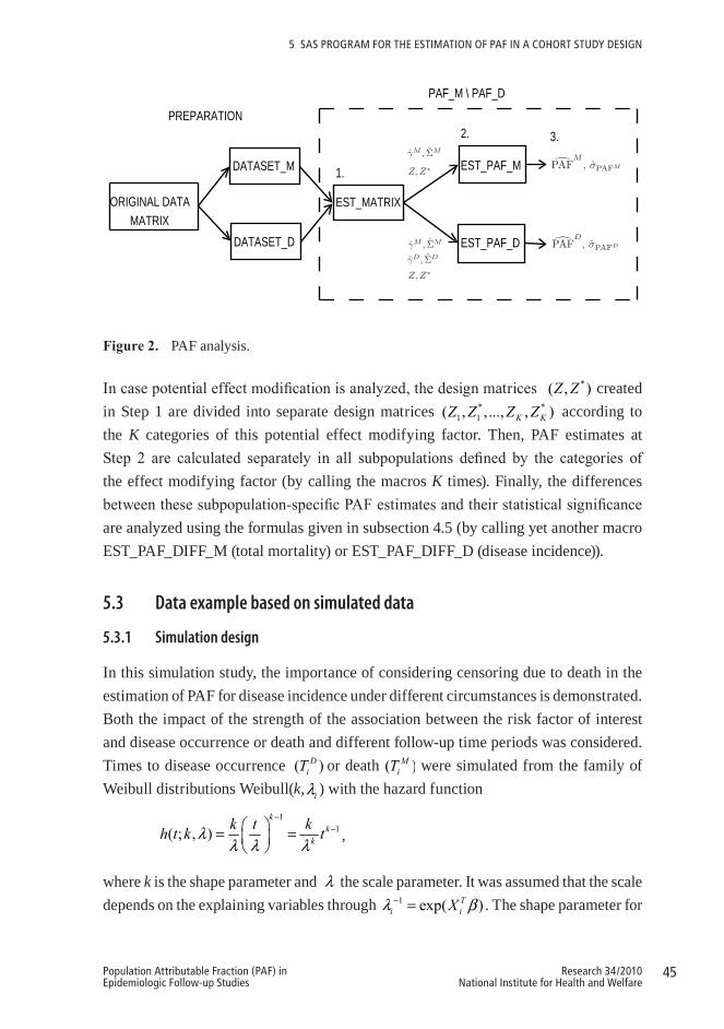
45Research 34/2010National Institute for Health and Welfare
Population Attributable Fraction (PAF) in Epidemiologic Follow-up Studies
5 SAS PRoGRAM FoR tHE EStIMAtIoN oF PAF IN A coHoRt StudY dESIGN
ORIGINAL DATA MATRIX
PREPARATION
DATASET_M
DATASET_D
EST_MATRIX
EST_PAF_M
EST_PAF_D
PAF_M \ PAF_D
1.
2. 3.γ̂M , Σ̂M
γ̂M , Σ̂M
γ̂D, Σ̂D
Z, Z∗
Z, Z∗
�PAFM
, σ̂PAFM
�PAFD
, σ̂PAFD
2
Figure2. PAF analysis.
In case potential effect modification is analyzed, the design matrices *( , )Z Z created in Step 1 are divided into separate design matrices * *
1 1( , ,..., , )K KZ Z Z Z according to the K categories of this potential effect modifying factor. Then, PAF estimates at Step 2 are calculated separately in all subpopulations defined by the categories of the effect modifying factor (by calling the macros K times). Finally, the differences between these subpopulation-specific PAF estimates and their statistical significance are analyzed using the formulas given in subsection 4.5 (by calling yet another macro EST_PAF_DIFF_M (total mortality) or EST_PAF_DIFF_D (disease incidence)).
5.3 Data example based on simulated data
5.3.1 Simulation design
In this simulation study, the importance of considering censoring due to death in the estimation of PAF for disease incidence under different circumstances is demonstrated. Both the impact of the strength of the association between the risk factor of interest and disease occurrence or death and different follow-up time periods was considered. Times to disease occurrence ( )DiT or death ( )M
iT were simulated from the family of Weibull distributions Weibull(k, iλ ) with the hazard function
11( ; , )
kk
k
k t kh t k tλλ λ λ
−−⎛ ⎞= =⎜ ⎟
⎝ ⎠,
where k is the shape parameter and λ the scale parameter. It was assumed that the scale depends on the explaining variables through 1 exp( )T
i iXλ β− = . The shape parameter for
46 Research 34/2010National Institute for Health and Welfare
Population Attributable Fraction (PAF) in Epidemiologic Follow-up Studies
5 SAS PRoGRAM FoR tHE EStIMAtIoN oF PAF IN A coHoRt StudY dESIGN
disease and death was allowed to be different. In this study, we consider one dichotomous risk factor X with RR = exp( )β . The values of 2 and 4 were chosen to represent relatively low and relatively high RRs, respectively, for both disease occurrence and death and all four relative risk combinations were studied. Datasets of n = 50 000 observations for the four different combinations of RRs were then simulated using the following scheme:
1. Draw X i ~ Bin(1, 0.5) and Age i ~ Uniform(40, 79) and round age to the nearest integer.
2. Fix the Weibull shape parameter to be kM = 2.1 for mortality and kD = 2.5 for disease occurrence. Determine the Weibull scale parameter as a function of age,
iMλ = 45 + (Age i − 40)(−1) for mortality and
iDλ = 100 + (Age i − 40)(−1.5) for
disease occurrence, to represent realistic baseline hazards for death and disease occurrence from 40 years on.
3. Simulate
( )1log *
Weibull , i
MM i
MMi M kRR XT k
e
λ⎛ ⎞⎜ ⎟⎜ ⎟⎝ ⎠
∼ and ( )1log *
Weibull , i
DD i
DDi D kRR XT k
e
λ⎛ ⎞⎜ ⎟⎜ ⎟⎝ ⎠
∼ ,
where RRM and RRD represent the RRs for mortality and disease occurrence when Xi = 1 in comparison to Xi = 0.
The follow-up time period was restricted to either 5, 10 or 20 years and the corresponding outcome variables for disease occurrence and death, indicating whether these events took place during those follow-up periods, were formed.
5.3.2 PAF analysis
After the four simulated datasets of n = 50 000 follow-up times until disease incidence or death, with the relative risk of the outcome being either 2 or 4, were prepared and the outcome variables, indicating whether disease or death occurred during the 5-, 10- or 20-year follow-up periods chosen, were formed, the PAF analysis could be carried out. First, the simulated data sets, which also included identification numbers for each observation, the binary risk factor, age, and the calculated birth year (assuming that this study was carried out in the year 2000), were prepared to fit the form required by
47Research 34/2010National Institute for Health and Welfare
Population Attributable Fraction (PAF) in Epidemiologic Follow-up Studies
5 SAS PRoGRAM FoR tHE EStIMAtIoN oF PAF IN A coHoRt StudY dESIGN
the PAF program, described in subsection 5.2. In preparing the data, 5-year follow-up time intervals and 10-year birth cohorts were used. Second, the point estimates of PAF, together with their 95% confidence intervals (CI) were calculated, using both the formulas for the estimation of PAF for disease incidence D
(0, ](PAF )t , which account for the censoring due to death, and the formulas for the estimation of PAF for total mortality M
(0, ](PAF )t , which ignore censoring due to death if outcomes other than death are used in them. It should be noted, however, that the hazard of the Weibull distribution, from which the follow-up times were drawn, is not piecewise constant as in the piecewise constant hazards model which was used in the estimation of M
(0, ]PAF t and D
(0, ]PAF t in Chapter 4. Finally, the PAF estimates obtained when either considering or ignoring censoring due to death for a certain follow-up t (here 5, 10, and 20 years) were compared.
5.3.3 Results
The differences in the results obtained using the two different PAF methods, one accounting for and one ignoring censoring due to death in the estimation of PAF for disease incidence, under different relative risks and follow-up time periods are substantial (Table 1). In general, the longer the follow-up time, and thus the greater the mortality, the more significant the effect of censoring due to death on the PAF estimates becomes. If the relative risk for mortality is small (RR=2), while the relative risk for disease incidence is equal or higher (RR=2 or RR=4), the consideration of censoring due to death results in significantly lower PAF estimates only when the follow-up time is long (t=20). If, on the other hand, the relative risk for mortality is high (RR=4), while the relative risk for disease incidence is equal or smaller (RR=4 or RR=2), the differences between the PAF estimates are already realized in a shorter follow-up time (t=10). If the risk factor has a stronger impact on death (RR=4) than on disease incidence (RR=2), the PAF estimates may even become negative (PAF = –5%, CI: –8%, –2%) when censoring due to death is taken into account. If censoring is not accounted for, the PAF equals 30% (CI: 28%, 33%). In summary, ignoring censoring due to death in the estimation of PAF for disease incidence leads to an overestimation of the proportion of preventable disease cases and thus to biased conclusions.
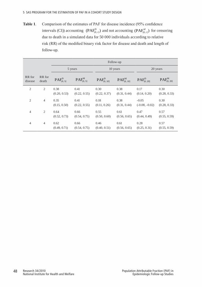
48 Research 34/2010National Institute for Health and Welfare
Population Attributable Fraction (PAF) in Epidemiologic Follow-up Studies
5 SAS PRoGRAM FoR tHE EStIMAtIoN oF PAF IN A coHoRt StudY dESIGN
Table1. Comparison of the estimates of PAF for disease incidence (95% confidence intervals (CI)) accounting D
(0, ](PAF )t and not accounting (0, ](PAF )Mt for censoring
due to death in a simulated data for 50 000 individuals according to relative risk (RR) of the modified binary risk factor for disease and death and length of follow-up.
RR for disease
RR for death
Follow-up
5 years 10 years 20 years
D(0, 5]PAF M
(0, 5]PAF D(0, 10]PAF M
(0, 10]PAF D(0, 20]PAF M
(0, 20]PAF
2 2 0.38 0.41 0.30 0.38 0.17 0.30(0.20, 0.53) (0.22, 0.55) (0.22, 0.37) (0.31, 0.44) (0.14, 0.20) (0.28, 0.33)
2 4 0.35 0.41 0.18 0.38 -0.05 0.30(0.15, 0.50) (0.22, 0.55) (0.11, 0.26) (0.31, 0.44) (-0.08, -0.02) (0.28, 0.33)
4 2 0.64 0.66 0.55 0.61 0.47 0.57(0.52, 0.73) (0.54, 0.75) (0.50, 0.60) (0.56, 0.65) (0.44, 0.49) (0.55, 0.59)
4 4 0.62 0.66 0.46 0.61 0.28 0.57(0.49, 0.71) (0.54, 0.75) (0.40, 0.51) (0.56, 0.65) (0.25, 0.31) (0.55, 0.59)

49Research 34/2010National Institute for Health and Welfare
Population Attributable Fraction (PAF) in Epidemiologic Follow-up Studies
6 RELATIVE IMPoRTAnCE oF THE MoDIFIABLE RISK FACToRS oF TYPE 2 DIABETES – An APPLICATIon oF PAF
The occurrence of type 2 diabetes is, mainly due to the ongoing obesity epidemic,
continuously growing worldwide (Wild et al. 2004). Besides obesity, other lifestyle factors, such as exercise, smoking, alcohol consumption, and some dietary habits (van Dam 2003), and combinations of these (Hu et al. 2001, Schulze et al. 2007, Mozaffarian et al. 2009) have also been shown to predict the occurrence of this disease. Recently it has been suggested that a low serum vitamin D concentration, related to lifestyle both through the diet (e.g. fish consumption) and outdoor activity (sunlight), may also predict the occurrence of type 2 diabetes (Pittas et al. 2006, Knekt et al. 2008).
Criteria of metabolic syndrome help to identify individuals at high risk for type 2 diabetes: the definition provided by the International Diabetes Federation (IDF) being the most recent (Alberti et al. 2006). Although the prediction of individual components of metabolic syndrome in this definition (i.e. waist circumference, blood pressure, serum HDL cholesterol, serum triglycerides and fasting glucose) on type 2 diabetes is well known (Hanson et al. 2002, Stern et al. 2002, Cheung et al. 2007), the risk attributable to the syndrome as a whole in a representative population sample has not been well described (Cheung et al. 2007, Cameron et al. 2008, Ford et al. 2008). In addition, a variety of risk scores combining factors related to lifestyle and metabolic syndrome have been proposed for identifying high-risk individuals (Stern et al. 2002, Lindstrom and Tuomilehto 2003, McNeely et al. 2003, Kanaya et al. 2005, Schmidt et al. 2005, Norberg et al. 2006).
It has been suggested that the role of lifestyle modification in reducing the incidence of type 2 diabetes is especially important in persons at high risk (Narayan et al. 2003, Schulze et al. 2007). Many intervention studies have also shown that positive changes in lifestyle, i.e. weight loss, increased exercise and improved diet, reduce the incidence of type 2 diabetes in high-risk individuals (Hu et al. 2006, Liberopoulos et al. 2006). However, a prediction of the modifiable lifestyle factors on the incidence of diabetes in individuals with and without metabolic syndrome has not yet been compared (Taslim and Tai 2009), and it is thus not known whether the effect of lifestyle modifications actually differs in high- and low-risk individuals.
50 Research 34/2010National Institute for Health and Welfare
Population Attributable Fraction (PAF) in Epidemiologic Follow-up Studies
6 RElAtIvE IMPoRtANcE oF tHE ModIFIABlE RISK FActoRS oF tYPE 2 dIABEtES – AN APPlIcAtIoN oF PAF
This study presents Population Attributable Fraction (PAF) estimates for modifiable lifestyle factors and components of the metabolic syndrome, and compares the expected importance of the lifestyle modification in persons with and without metabolic syndrome in a pooled sample of two representative Finnish cohorts.
6.1 Populations and measurement methods
6.1.1 Study populations
The data in this study were based on two cohorts, the Mini-Finland Health Survey (MFH) carried out in 1978–1980 (Aromaa et al. 1989) and the Health 2000 Survey (Health 2000) carried out in 2000–2001 (Aromaa and Koskinen 2004). Both samples were stratified two-stage cluster samples, representative of the Finnish adult population aged 30 years and over. The MFH sample comprised 8,000 individuals from 40 geographical areas, and the Health 2000 sample 8,028 individuals from 80 areas. A total of 7,217 subjects (90% of the sample) in the MFH sample and 6,771 subjects (84% of the sample) in the Health 2000 sample participated in a health examination. Persons aged 40–79 years and free of type 2 diabetes and cardiovascular diseases at baseline were included in this study. The final data comprised a total of 4,517 individuals (2,004 men and 2,513 women) from the MFH sample and 4,110 individuals (1,850 men and 2,260 women) from Health 2000 sample.
6.1.2 Risk assessment
VariablesconsideredData on education, smoking, leisure time exercise, alcohol consumption, previous diseases (e.g. type 2 diabetes and cardiovascular diseases), and antihypertensive medication were self-reported in a health interview or a self-administered questionnaire at baseline. Height and weight were measured at a health examination, and body mass index (BMI) was calculated. Waist circumference was measured in Health 2000 only. Casual blood pressure was measured twice with a 1.5 minute interval in both populations by the auscultatory method, and fasting blood samples were taken and stored at –20 °C (MFH) or –70 °C (Health 2000). Serum HDL cholesterol, serum triglycerides, and fasting glucose levels were determined as soon as technically possible (usually some weeks) after the samples were taken. Serum HDL cholesterol was analyzed using Mg-dextrane sulphate precipitation in MFH (Kostner 1976) and using a direct method in Health 2000 (HDL-C Plus, Roche Diagnostics, Germany). Serum triglyceride

51Research 34/2010National Institute for Health and Welfare
Population Attributable Fraction (PAF) in Epidemiologic Follow-up Studies
6 RElAtIvE IMPoRtANcE oF tHE ModIFIABlE RISK FActoRS oF tYPE 2 dIABEtES – AN APPlIcAtIoN oF PAF
concentration was determined fully enzymatically (MFH: Boehringer, Mannheim, Germany; Health 2000: Olympus System Reagent, Germany). Plasma samples were used for glucose analysis in MFH (glucose oxidase, Boehringer Mannheim, Germany) and serum samples in Health 2000 (hexokinase, Olympus System Reagent, Germany). Serum vitamin D concentrations (serum 25-hydroxyvitamin D) were determined in 2001–2004 using radioimmunoassay (RIA, DiaSorin, Minnesota). Every variable was standardized between the two cohorts to the greatest extent possible.
Low-risklifestyleFive modifiable lifestyle factors were used to define a low-risk lifestyle level, i.e. BMI, exercise, smoking, alcohol consumption, and serum vitamin D. Low risk was defined as a BMI < 25.0 kg/m2, occasional or regular exercise (3–4 hours per week, i.e. approximately 30 minutes per day), not smoking, alcohol consumption of 1–99g/week in women and 1–199g/week in men, and a serum vitamin D level above the median ( > 39 nmol/l in MFH and > 44 nmol/l in Health 2000).
ThemetabolicsyndromeThe metabolic syndrome was, according to the International Diabetes Federation (IDF) (Alberti et al. 2006), defined as waist circumference ≥ 94 cm in men and ≥ 80 cm in women together with an unsatisfactory value in at least two of the following variables: blood pressure, serum HDL cholesterol, serum triglycerides, and fasting glucose. Unsatisfactory values were defined as follows: blood pressure was considered elevated if the mean level of two systolic blood pressure measurements was ≥ 130 mmHg or the mean level of two diastolic blood pressure measurements was ≥ 85 mmHg or antihypertensive medication was used; low serum HDL cholesterol included serum values ≤ 1.02 mmol/l in men and ≤ 1.29 mmol/l in women; serum triglycerides were considered elevated if the serum value was ≥ 1.7 mmol/l; fasting glucose was elevated if it was ≥ 5.6 mmol/l. Since waist circumference was not measured in MFH, a BMI ≥ 25 kg/m2 was used as its proxy measure in definition of metabolic syndrome (IDF criteria). The relative risk (95% CI) of diabetes for individuals with metabolic syndrome according to the original definition and the proxy definition in Health 2000 were 6.70 (3.61, 12.4) and 6.78 (3.72, 12.4), respectively. The corresponding PAF values were 0.71 (0.52, 0.83) and 0.71 (0.52, 0.82).
52 Research 34/2010National Institute for Health and Welfare
Population Attributable Fraction (PAF) in Epidemiologic Follow-up Studies
6 RElAtIvE IMPoRtANcE oF tHE ModIFIABlE RISK FActoRS oF tYPE 2 dIABEtES – AN APPlIcAtIoN oF PAF
6.1.3 Diabetes incidence
A cohort study design with type 2 diabetes incidence as the outcome was adopted. Under the Sickness Insurance Act, all diabetics needing drug therapy are entitled to reimbursement of drug costs, eligibility for which requires a detailed medical certificate from an attending physician (Reunanen et al. 2000). A central register of all patients receiving drug reimbursement is kept by the Social Insurance Institution. Participants in the cohorts of the present study were linked to this register by the unique code assigned to each Finnish citizen. All medical certificates of these cases were checked to ensure that they meet the WHO diagnostic criteria for type 2 diabetes mellitus (World Health Organization 1985). In addition, disease events leading to hospitalization were identified by linking data from the Finnish Hospital Discharge Register (Heliövaara et al. 1984). Furthermore, information on mortality was based on death certificates obtained from Statistics Finland (Reunanen et al. 1983), and the individuals with type 2 diabetes cited as the principal cause of death were classified as diabetes cases. The follow-up time was defined as the number of days from the baseline examination to the date of type 2 diabetes occurrence, death, or end of follow-up, whichever came first. The follow-up time was 10 years in MFH and 7 years in Health 2000. During the follow-up times, a total of 145 individuals in MFH and 81 in Health 2000 developed type 2 diabetes.
6.2 Statistical methods
6.2.1 Cohort-specific analyses
A piecewise constant hazards model (Friedman 1982) was used to assess the Population Attributable Fraction (PAF) (4.11) for the potential risk factors of type 2 diabetes incidence. Two-sided 95% confidence intervals (CI) for PAF were estimated using the delta method and by applying a symmetrizing complementary logarithmic transformation of PAF (4.16). To avoid assumptions about the shape of the relationship between the potential continuous risk factors and the incidence of type 2 diabetes in the statistical analyses, RRs and PAFs were estimated for categories of these variables. Cox’s model (Cox 1972) was used to assess the relative risk (RR).
Two main effects models were defined. The first model (both RR and PAF) included age, sex, and separately each of the five lifestyle factors (i.e. BMI, physical exercise, smoking, alcohol consumption, and serum vitamin D), or each of the components
53Research 34/2010National Institute for Health and Welfare
Population Attributable Fraction (PAF) in Epidemiologic Follow-up Studies
6 RElAtIvE IMPoRtANcE oF tHE ModIFIABlE RISK FActoRS oF tYPE 2 dIABEtES – AN APPlIcAtIoN oF PAF
of metabolic syndrome (i.e. BMI, blood pressure, serum HDL cholesterol, serum triglycerides, and fasting glucose), or metabolic syndrome as a whole. The second model (only PAF) included age, sex, and combinations of lifestyle factors or components of metabolic syndrome adjusted for the factors not included in the combination.
Possible modifications by sex, age, metabolic syndrome or its components on the prediction of the lifestyle factors on type 2 diabetes risk were studied by including an interaction term between the risk factor or combination of risk factors of interest and the potential effect modifying factor in the model. The statistical significance of effect modification was studied by calculating the 95% confidence interval (CI) of the difference of the PAF estimates between the categories of the effect modifying factor using the delta method (4.18).
6.2.2 Pooling
The sub-cohort specific logs of RRs or complementary-log transformed PAFs or untransformed PAF differences were combined, weighting them by the inverse of their variance, in a random-effects model using formula (4.19) (DerSimonian and Laird 1986). Heterogeneity among the study-specific RRs or PAFs was tested using the asymptotic DerSimonian and Laird Q statistic (DerSimonian and Laird 1986). The potential heterogeneity due to sex was tested by the Wald test (Stram 1996).
The calculations were performed using the SAS procedures PHREG, TPHREG, LIFEREG, MIXED and IML (SAS Institute Inc. 2007).
6.3 Results
6.3.1 Description of the study populations
During the 20-year period between the MFH and Health 2000 the educational level in Finland rose and the proportion of persons occasionally or regularly exercising increased (Table 2). Of the components of the metabolic syndrome, both blood pressure and serum HDL cholesterol improved. At the same time, however, the Finnish population became more obese and heavy use of alcohol increased. The relative risk of diabetes during a 10-year follow-up from baseline did not differ between the two samples, with the exception of the fasting glucose level (Original publication IV).
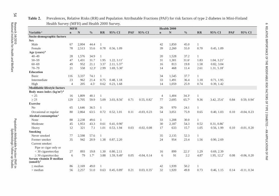
54Research 34/2010N
ational Institute for Health and W
elfarePopulation Attributable Fraction (PA
F) in Epidem
iologic Follow-up Studies
6 RElAtIvE IMPo
RtAN
cE oF tH
E Mo
dIFIA
BlE RISK FActoRS o
F tYPE 2 dIA
BEtES – AN
APPlIcAtIo
N o
F PAF
Table2. Prevalences, Relative Risks (RR) and Population Attributable Fractions (PAF) for risk factors of type 2 diabetes in Mini-Finland Health Survey (MFH) and Health 2000 Survey.
MFH Health2000Variablea n N % RR 95% CI PAF 95% CI n N % RR 95% CI PAF 95% CISocio-demographicfactorsSex Male 67 2,004 44.4 1 42 1,850 45.0 1 Female 78 2,513 55.6 0.78 0.56, 1.09 39 2,260 55.0 0.70 0.45, 1.09Age(years)b 40–49 28 1,576 34.9 1 20 1,528 37.2 1 50–59 47 1,431 31.7 1.95 1.22, 3.11* 31 1,301 31.6c 1.83 1.04, 3.21*
60–69 49 952 21.1 3.37 2.11, 5.37* 16 813 19.8 1.58 0.82, 3.04 70–79 21 558 12.3c 2.99 1.69, 5.30* 14 468 11.4 2.61 1.31, 5.18*
Education Basic 116 3,337 74.1 1 34 1,545 37.7 1 Intermediate 23 962 21.4 0.75 0.48, 1.18 33 1,491 36.4 1.18 0.71, 1.95 High 4 205 4.5c 0.62 0.23, 1.68 14 1,059 25.9 0.74 0.39, 1.42ModifiablelifestylefactorsBodymassindex(kg/m2)d < 25 16 1,809 40.1 1 4 1,404 34.3c 1 ≥ 25 129 2,705 59.9 5.09 3.03, 8.56* 0.71 0.55, 0.82* 77 2,695 65.7c 9.36 3.42, 25.6* 0.84 0.59, 0.94*
Exercise No 65 1,646 36.5 1 26 970 24.1 1 Occasional or regular 80 2,864 63.5 0.72 0.52, 1.01 0.11 -0.03, 0.23 54 3,051 75.9 0.65 0.40, 1.03 0.10 -0.04, 0.23Alcoholconsumptione None 88 2,238 49.6 1 33 1,208 30.0 1 Moderate 45 1,953 43.3 0.61 0.41, 0.90* 30 2,187 54.3 0.52 0.31, 0.86*
Heavy 12 321 7.1 1.01 0.53, 1.94 0.03 -0.02, 0.08 17 633 15.7 1.05 0.56, 1.99 0.10 -0.01, 0.20Smoking Never smoked 77 2,598 57.6 1 35 2,135 52.3 1 Former smoker 35 942 20.9 1.38 0.87, 2.20 24 954 23.4 1.56 0.90, 2.69 Current smoker: Pipe or cigar only or < 30 cigarettes/day 27 893 19.8 1.30 0.80, 2.11 16 899 22.1c 1.29 0.69, 2.39 ≥ 30 cigarettes/day 6 79 1.7c 3.88 1.59, 9.49* 0.05 -0.04, 0.14 6 91 2.2 4.87 1.95, 12.2* 0.08 -0.06, 0.20SerumvitaminDmedian (nmol/l)f
≤ median 86 2,169 49.0 1 42 1,939 50.2 1 > median 56 2,257 51.0 0.63 0.45, 0.89* 0.21 0.03, 0.35* 32 1,920 49.8 0.73 0.46, 1.15 0.14 -0.11, 0.34
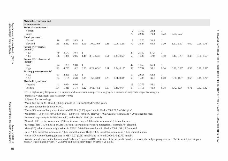
55Research 34/2010
National Institute for H
ealth and Welfare
Population Attributable Fraction (PAF) in
Epidemiologic Follow
-up Studies
6 RElAtIvE IMPo
RtAN
cE oF tH
E Mo
dIFIA
BlE RISK FActoRS o
F tYPE 2 dIA
BEtES – AN
APPlIcAtIo
N o
F PAF
Metabolicsyndromeand itscomponentsWaistcircumferenceg Normal 2 1,150 28.2 1 Large 79 2,932 71.8 15.2 3.74, 62.2*
Bloodpressureh Normal 10 653 14.5 1 9 1,270 31.0 1 Elevated 135 3,262 85.5 1.93 1.00, 3.69* 0.41 -0.08, 0.68 72 2,827 69.0 3.20 1.57, 6.50* 0.60 0.26, 0.78*
Serumtriglycerides (mmol/l)i < 1.7 49 3,177 70.4 1 27 2,750 67.2c 1 ≥ 1.7 96 1,338 29.6 4.46 3.15, 6.31* 0.51 0.38, 0.60* 53 1,339 32.8c 3.90 2.44, 6.23* 0.48 0.30, 0.62*
SerumHDLcholesterol (mmol/l)j Low 24 281 93.8 1 47 1,355 66.9 1 High 121 4,233 6.2 0.33 0.21, 0.51* 0.11 0.04, 0.17* 33 2,734 33.1 0.34 0.22, 0.53* 0.38 0.20, 0.52*
Fastingglucose(mmol/l)k < 5.6 81 3,350 74.2 1 17 2,654 64.9 1 ≥ 5.6 64 1,165 25.8 2.15 1.55, 3.00* 0.23 0.11, 0.33* 63 1,435 35.1 6.70 3.88, 11.6* 0.65 0.48, 0.77*
Metabolicsyndromel Negative 41 3,094 68.6 1 13 2,379 58.1 1 Positive 104 1,419 31.4 5.22 3.62, 7.52* 0.57 0.45, 0.67* 67 1,715 41.9 6.78 3.72, 12.4* 0.71 0.52, 0.82*
HDL = high-density lipoprotein, n = number of disease cases in respective category, N = number of subjects in respective category* Statistically significant association (P < 0.05)a Adjusted for sex and age.b Mean (SD) age in MFH 55.3 (10.4) years and in Health 2000 54.7 (10.2) years.c Per cents rounded to sum up to 100.d Mean (SD) value of body mass index in MFH 26.4 (3.98) kg/m2 and in Health 2000 27.2 (4.56) kg/m2.e Moderate: 1–99g/week for women and 1–199g/week for men. Heavy: ≥ 100g/week for women and ≥ 200g/week for men.f Evaluated separately in MFH (39 nmol/l) and in Health 2000 (44 nmol/l).g Normal: < 80 cm for women and < 94 cm for men. Large: ≥ 80 cm for women and ≥ 94 cm for men.h Elevated: SBP ≥ 130 mmHg or DBP ≥ 85 mmHg or antihypertensive medication. Normal: Not elevated.i Mean (SD) value of serum triglycerides in MFH 1.54 (0.85) mmol/l and in Health 2000 1.59 (1.02) mmol/l.j Low: ≤ 1.29 mmol/l in women and ≤ 1.02 mmol/l in men. High: > 1.29 mmol/l in women and > 1.02 mmol/l in men.k Mean (SD) value of fasting glucose in MFH 5.27 (0.59) mmol/l and in Health 2000 5.45 (0.75) mmol/l.l Waist circumference in the International Diabetes Federation (IDF) definition of the metabolic syndrome was replaced by a proxy measure BMI in which the category normalg was replaced by BMI < 25 kg/m2 and the category largeg by BMI ≥ 25 kg/m2.
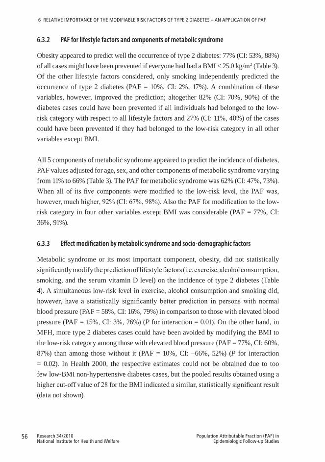
56 Research 34/2010National Institute for Health and Welfare
Population Attributable Fraction (PAF) in Epidemiologic Follow-up Studies
6 RElAtIvE IMPoRtANcE oF tHE ModIFIABlE RISK FActoRS oF tYPE 2 dIABEtES – AN APPlIcAtIoN oF PAF
6.3.2 PAF for lifestyle factors and components of metabolic syndrome
Obesity appeared to predict well the occurrence of type 2 diabetes: 77% (CI: 53%, 88%) of all cases might have been prevented if everyone had had a BMI < 25.0 kg/m2 (Table 3). Of the other lifestyle factors considered, only smoking independently predicted the occurrence of type 2 diabetes (PAF = 10%, CI: 2%, 17%). A combination of these variables, however, improved the prediction; altogether 82% (CI: 70%, 90%) of the diabetes cases could have been prevented if all individuals had belonged to the low-risk category with respect to all lifestyle factors and 27% (CI: 11%, 40%) of the cases could have been prevented if they had belonged to the low-risk category in all other variables except BMI.
All 5 components of metabolic syndrome appeared to predict the incidence of diabetes, PAF values adjusted for age, sex, and other components of metabolic syndrome varying from 11% to 66% (Table 3). The PAF for metabolic syndrome was 62% (CI: 47%, 73%). When all of its five components were modified to the low-risk level, the PAF was, however, much higher, 92% (CI: 67%, 98%). Also the PAF for modification to the low-risk category in four other variables except BMI was considerable (PAF = 77%, CI: 36%, 91%).
6.3.3 Effect modification by metabolic syndrome and socio-demographic factors
Metabolic syndrome or its most important component, obesity, did not statistically significantly modify the prediction of lifestyle factors (i.e. exercise, alcohol consumption, smoking, and the serum vitamin D level) on the incidence of type 2 diabetes (Table 4). A simultaneous low-risk level in exercise, alcohol consumption and smoking did, however, have a statistically significantly better prediction in persons with normal blood pressure (PAF = 58%, CI: 16%, 79%) in comparison to those with elevated blood pressure (PAF = 15%, CI: 3%, 26%) (P for interaction = 0.01). On the other hand, in MFH, more type 2 diabetes cases could have been avoided by modifying the BMI to the low-risk category among those with elevated blood pressure (PAF = 77%, CI: 60%, 87%) than among those without it (PAF = 10%, CI: –66%, 52%) (P for interaction = 0.02). In Health 2000, the respective estimates could not be obtained due to too few low-BMI non-hypertensive diabetes cases, but the pooled results obtained using a higher cut-off value of 28 for the BMI indicated a similar, statistically significant result (data not shown).
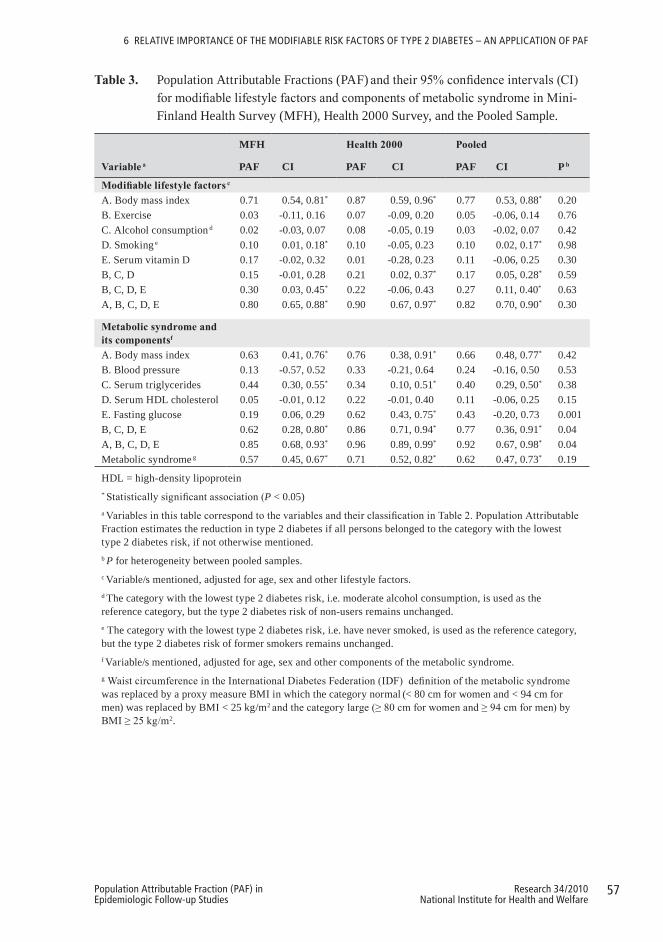
57Research 34/2010National Institute for Health and Welfare
Population Attributable Fraction (PAF) in Epidemiologic Follow-up Studies
6 RElAtIvE IMPoRtANcE oF tHE ModIFIABlE RISK FActoRS oF tYPE 2 dIABEtES – AN APPlIcAtIoN oF PAF
Table3. Population Attributable Fractions (PAF) and their 95% confidence intervals (CI) for modifiable lifestyle factors and components of metabolic syndrome in Mini-Finland Health Survey (MFH), Health 2000 Survey, and the Pooled Sample.
Variablea
MFH Health2000 Pooled
P bPAF CI PAF CI PAF CI
Modifiablelifestylefactorsc
A. Body mass index 0.71 0.54, 0.81* 0.87 0.59, 0.96* 0.77 0.53, 0.88* 0.20B. Exercise 0.03 -0.11, 0.16 0.07 -0.09, 0.20 0.05 -0.06, 0.14 0.76C. Alcohol consumption d 0.02 -0.03, 0.07 0.08 -0.05, 0.19 0.03 -0.02, 0.07 0.42D. Smoking e 0.10 0.01, 0.18* 0.10 -0.05, 0.23 0.10 0.02, 0.17* 0.98E. Serum vitamin D 0.17 -0.02, 0.32 0.01 -0.28, 0.23 0.11 -0.06, 0.25 0.30B, C, D 0.15 -0.01, 0.28 0.21 0.02, 0.37* 0.17 0.05, 0.28* 0.59B, C, D, E 0.30 0.03, 0.45* 0.22 -0.06, 0.43 0.27 0.11, 0.40* 0.63A, B, C, D, E 0.80 0.65, 0.88* 0.90 0.67, 0.97* 0.82 0.70, 0.90* 0.30
Metabolicsyndromeand itscomponentsf
A. Body mass index 0.63 0.41, 0.76* 0.76 0.38, 0.91* 0.66 0.48, 0.77* 0.42B. Blood pressure 0.13 -0.57, 0.52 0.33 -0.21, 0.64 0.24 -0.16, 0.50 0.53C. Serum triglycerides 0.44 0.30, 0.55* 0.34 0.10, 0.51* 0.40 0.29, 0.50* 0.38D. Serum HDL cholesterol 0.05 -0.01, 0.12 0.22 -0.01, 0.40 0.11 -0.06, 0.25 0.15E. Fasting glucose 0.19 0.06, 0.29 0.62 0.43, 0.75* 0.43 -0.20, 0.73 0.001B, C, D, E 0.62 0.28, 0.80* 0.86 0.71, 0.94* 0.77 0.36, 0.91* 0.04A, B, C, D, E 0.85 0.68, 0.93* 0.96 0.89, 0.99* 0.92 0.67, 0.98* 0.04Metabolic syndrome g 0.57 0.45, 0.67* 0.71 0.52, 0.82* 0.62 0.47, 0.73* 0.19
HDL = high-density lipoprotein* Statistically significant association (P < 0.05)a Variables in this table correspond to the variables and their classification in Table 2. Population Attributable Fraction estimates the reduction in type 2 diabetes if all persons belonged to the category with the lowest type 2 diabetes risk, if not otherwise mentioned.b P for heterogeneity between pooled samples.c Variable/s mentioned, adjusted for age, sex and other lifestyle factors.d The category with the lowest type 2 diabetes risk, i.e. moderate alcohol consumption, is used as the reference category, but the type 2 diabetes risk of non-users remains unchanged.e The category with the lowest type 2 diabetes risk, i.e. have never smoked, is used as the reference category, but the type 2 diabetes risk of former smokers remains unchanged.f Variable/s mentioned, adjusted for age, sex and other components of the metabolic syndrome.g Waist circumference in the International Diabetes Federation (IDF) definition of the metabolic syndrome was replaced by a proxy measure BMI in which the category normal (< 80 cm for women and < 94 cm for men) was replaced by BMI < 25 kg/m2 and the category large (≥ 80 cm for women and ≥ 94 cm for men) by BMI ≥ 25 kg/m2.
58 Research 34/2010National Institute for Health and Welfare
Population Attributable Fraction (PAF) in Epidemiologic Follow-up Studies
6 RElAtIvE IMPoRtANcE oF tHE ModIFIABlE RISK FActoRS oF tYPE 2 dIABEtES – AN APPlIcAtIoN oF PAF
Table4. Population Attributable Fractions (PAF) and their 95% confidence intervals (CI) for modifiable lifestyle factors of type 2 diabetes by categories of potential effect modifying factors and the statistical significance of their differences in a pooled sample of Mini-Finland Health Survey (MFH) and Health 2000 Survey.
Variablea,b
Effectmodifyingfactor
P for interaction
CategoryA CategoryB
PAFA CI PAFB CI
Metabolicsyndrome:A=No B=YesB. Exercise -0.01 -0.19, 0.15 0.08 -0.04, 0.18 0.44C. Alcohol consumptionc -0.02 -0.15, 0.10 0.06 -0.04, 0.16 0.39D. Smokingd 0.09 -0.08, 0.24 0.07 -0.01, 0.15 0.78E. Serum vitamin D 0.04 -0.26, 0.27 0.16 -0.02, 0.30 0.35B, C, D 0.20 0.03, 0.34* 0.06 -0.19, 0.27 0.77B, C, D, Ee 0.13 -0.31, 0.43 0.29 0.03, 0.48* 0.47
Sex:A=Men B=WomenA. Body mass index 0.77 0.57, 0.88* 0.79 0.11, 0.95* 0.74B. Exercise 0.07 -0.06, 0.19 0.12 -0.03, 0.24 0.70C. Alcohol consumptionc 0.09 -0.00, 0.17 0.01 -0.06, 0.08 0.08D. Smoking d 0.12 -0.03, 0.24 0.04 -0.04, 0.11 0.33E. Serum vitamin D 0.04 -0.15, 0.20 0.33 0.12, 0.50* 0.02B, C, D 0.22 0.04, 0.36* 0.17 0.01, 0.30* 0.61B, C, D, E 0.22 -0.02, 0.40 0.38 0.15, 0.55* 0.32A, B, C, D, E 0.83 0.65, 0.92* 0.83 0.63, 0.92* 0.80
Age:A=40–59years B=60–79yearsA. Body mass index 0.77 0.48, 0.90* 0.73 0.49, 0.85* 0.74B. Exercise 0.13 -0.00, 0.24 0.07 -0.09, 0.20 0.57C. Alcohol consumption c 0.06 -0.04, 0.15 0.02 -0.02, 0.06 0.43D. Smoking d 0.16 0.04, 0.27* -0.04 -0.12, 0.03 0.002E. Serum vitamin D 0.11 -0.08, 0.26 0.29 0.06, 0.46* 0.15B, C, D 0.27 0.12, 0.40* 0.06 -0.12, 0.22 0.06B, C, D, E 0.32 0.12, 0.47* 0.25 -0.03, 0.46 0.71A, B, C, D, E 0.87 0.50, 0.97* 0.79 0.57, 0.90* 0.67* Statistically significant association (P < 0.05)aAdjusted for sex and age.b Variables in this table correspond to the variables and their classification in Table 2. Population Attributable Fraction estimates the reduction in type 2 diabetes if all persons belonged to the category with the lowest type 2 diabetes risk, if not mentioned otherwise.c The category with the lowest type 2 diabetes risk, i.e. moderate alcohol consumption, is used as the reference category, but the type 2 diabetes risk of non-users remains unchanged.d The category with the lowest type 2 diabetes risk, i.e. have never smoked, is used as the reference category, but the type 2 diabetes risk of former smokers remains unchangede Pooled effect modification analysis could not be carried out due to too few diabetes cases in some low-risk strata of Health 2000 data, and therefore these figures derive from the MFH data.

59Research 34/2010National Institute for Health and Welfare
Population Attributable Fraction (PAF) in Epidemiologic Follow-up Studies
6 RElAtIvE IMPoRtANcE oF tHE ModIFIABlE RISK FActoRS oF tYPE 2 dIABEtES – AN APPlIcAtIoN oF PAF
Study of the interactions between lifestyle and socio-demographic factors (i.e. sex and age) showed that belonging to the low-risk category for smoking had a stronger prediction on reduction of type 2 diabetes in younger persons (P for interaction = 0.002) and having higher serum vitamin D a stronger prediction in women (P for interaction = 0.02).
In summary, this study showed that weight control is the primary diabetes prevention method and that adequate exercise, moderate alcohol consumption, not smoking, and a satisfactory vitamin D level also play an important role. Metabolic syndrome did not modify the prediction of lifestyle factors. However, of its single components, blood pressure did modify the prediction: individuals with elevated blood pressure apparently benefit less from positive changes in exercise, smoking, or alcohol consumption.
60 Research 34/2010National Institute for Health and Welfare
Population Attributable Fraction (PAF) in Epidemiologic Follow-up Studies
7 DISCUSSIon
7.1 Main findings
7.1.1 Statistical method and program for the estimation of PAF for total mortality and disease incidence in a cohort study design
Methods that properly take into account the time perspective in the estimation of Population Attributable Fraction (PAF) in cohort studies with censored time-to-event data have been developed during recent years (Chen et al. 2006, Samuelsen and Eide 2008, Cox et al. 2009). Censoring during follow-up may result from different sources. If the event of interest is death, censoring due to end of follow-up or loss to follow-up needs to be considered. If the event of interest is the incidence of a specific disease, censoring due to death due to reasons other than the event of interest also needs to be considered. Ignoring censoring due to death leads to potentially biased estimates, as an unrealistic assumption of no one dying during the follow-up is made in the estimation. So far, censoring due to death has only been considered in single studies (Silverberg et al. 2004, Samuelsen and Eide 2008), but the definition of PAF for disease incidence has not been generalized to account for censoring due to death. In this study, the PAF was defined as the proportion of mortality or disease incidence that could be avoided during a time interval (0, t] if their risk factors were modified. In the definition of PAF for disease incidence, censoring due to death was taken into account. Thus, the interest was in the order of occurrence of disease and death. The times to death or disease incidence were assumed to follow a proportional hazards model with piecewise constant baseline hazard functions, independently given the risk factors X. Maximum likelihood estimation was used to obtain the point estimates of PAF. Taking censoring due to death into account in the estimation was shown to decrease the point estimates of PAF in comparison to methods which ignored censoring due to death. This bias was greater when the impact of risk factors on mortality was stronger and when the follow-up time was longer. The bias became even clearer when the cumulative effect of the modification of several risk factors on disease incidence was analyzed (Original Publication II). The formulas and estimation methods of PAF for total mortality and disease incidence provided in this study can also be applied for the estimation of PAF for other types of inevitable and not inevitable events, and accounting also for censoring due to competing risks other than just death.
61Research 34/2010National Institute for Health and Welfare
Population Attributable Fraction (PAF) in Epidemiologic Follow-up Studies
7 dIScuSSIoN
So far, the estimation of PAF for the time interval (0, t] has usually been carried out using the Cox proportional hazards model with the Breslow estimator for the cumulative baseline hazard (Chen et al. 2006, Samuelsen and Eide 2008). The variance of PAF estimates has either been been derived asymptotically (Chen et al. 2006) or it has been obtained using resampling-based methods, such as bootstrap (Samuelsen and Eide 2008). The resampling-based methods, despite having the advantage of simplicity over analytic methods, are very time-consuming in terms of computing resources. In this study, asymptotic variance estimation of PAF applying the delta method based on the fully parametrized piecewise constant hazards model was carried out.
The exposure-outcome relationship, and thus PAF, is affected by confounding and effect modification. In the model-based estimation presented in this study, potential confounding factors were adjusted for and effect modifying factors accounted for by including them in the model. In this study, new model-based methods for the analysis of PAF in the subpopulations defined by categories of potential effect modifying factors and determination of the statistical significance of the differences between these subpopulation-specific PAF estimates in a cohort study design were developed.
The pooling of different cohorts is becoming increasingly common. Pooled PAF estimates so far presented in the literature have, however, been calculated by inserting the adjusted RR derived from meta-analysis and the average prevalence of the risk factor across individual studies in some of the PAF formulas presented in the literature (Olsen et al. 2010). In this study, the pooling methodology presented and applied in the literature for pooling relative risks (Knekt et al. 2004, Smith-Warner et al. 2006) was generalized to apply for pooling PAF estimates, and pooled PAF estimates based on the new formulas provided in this study were presented. The need for publicly available programs for the estimation of PAF has been acknowledged in the literature (Benichou 2001), but only one program for the estimation of PAF in a cohort study design has been presented (Spiegelman et al. 2007). This program, however, produces static PAF estimates over time considering censoring due to loss to follow-up in the estimation of PAF. No publicly available programs thus exist for the estimation of the dynamic PAF for a certain time interval, and taking censoring due to competing risks, such as death, into account when the outcome of interest is not an inevitable event, such as a specific disease. In this study, a SAS-based program for the estimation of PAF in a cohort study design, both for total mortality and for disease incidence, considering censoring due to death, was presented.
62 Research 34/2010National Institute for Health and Welfare
Population Attributable Fraction (PAF) in Epidemiologic Follow-up Studies
7 dIScuSSIoN
7.1.2 Application of PAF for the analysis of the relative importance of the risk factors of type 2 diabetes
There seems to be a gap between theory and the practice of PAF in the literature. Although the estimation of PAF from different designs has become more thoroughly covered in statistical and biometrical journals since the 1970s, there are still relatively few applications using PAF, especially in cohort studies. In this study, the new methodology and program presented for the estimation of PAF in a cohort study design was applied to estimate the relative importance of lifestyle factors and components of metabolic syndrome as well as the potential effect modification by metabolic syndrome on the incidence of type 2 diabetes in a pooled sample of two representative Finnish cohorts.
Over 80% of all incident diabetes cases occurring in these two cohorts could be attributed to failure to follow a low-risk lifestyle, including a body mass index under 25, adequate exercise, moderate alcohol consumption, not smoking, and a satisfactory vitamin D level. This suggests that the majority of type 2 diabetes cases could be avoided by modifications of lifestyle, which is in line with previous findings (Hu et al. 2001, Schulze et al. 2007, Mozaffarian et al. 2009). Obesity was the most important predictor of type 2 diabetes. Accordingly, and in line with previous cohort (Hu et al. 2001, Schulze et al. 2007, Mozaffarian et al. 2009) and intervention (Schulze and Hu 2005, Liberopoulos et al. 2006) studies, weight control would apparently be the most important strategy for type 2 diabetes prevention. The four other lifestyle variables were also significantly associated with an increased risk of diabetes, in agreement with previous studies (Hu et al. 2001, Mozaffarian et al. 2009). At the population level, however, only one fourth of the incident disease cases seemed attributable to all four variables combined; smoking being the only single variable significantly associated with a reduced diabetes risk.
Two thirds of the disease cases could be attributed to having metabolic syndrome, which is in agreement with the fact that metabolic syndrome is a strong predictor of type 2 diabetes (Cheung et al. 2007, Ford et al. 2008). All five single components of metabolic syndrome (i.e. waist circumference or BMI, blood pressure, serum HDL cholesterol, serum triglycerides, and fasting glucose) also predicted the occurrence of type 2 diabetes, which is also in accordance with previous cohort (Cheung et al. 2007, Hanson et al. 2002) and intervention (Liberopoulos et al. 2006, Schulze et al. 2005) studies. In fact, over 90% of all cases could have been avoided if all individuals had belonged to the low-risk category in all five components of metabolic syndrome.
63Research 34/2010National Institute for Health and Welfare
Population Attributable Fraction (PAF) in Epidemiologic Follow-up Studies
7 dIScuSSIoN
The potential effect modification of metabolic syndrome on the prediction of lifestyle modifications for the incidence of type 2 diabetes was explored for the first time in the present study. No interactions between lifestyle and metabolic syndrome were, however, found. It appeared, however, that positive changes in smoking, alcohol consumption and exercise could have prevented more type 2 diabetes cases among persons with normal blood pressure than among persons with elevated blood pressure. This result thus contradicts the frequent claim that lifestyle modifications have a greater effect in high-risk individuals (Narayan et al. 2003). Reducing the BMI, on the other hand, was more strongly associated with a reduced diabetes risk in persons with elevated blood pressure than in persons without it. This result is consistent with the finding that weight reduction had a stronger effect on the incidence of type 2 diabetes in high-risk individuals than in low-risk individuals (Knowler et al. 2002, Orchard et al. 2005). Overall, lifestyle factors not involved in metabolic syndrome seem to play a more important role in the prevention of type 2 diabetes in low-risk individuals. Therefore, as regards the constantly growing diabetes epidemic, it is important to target lifestyle-related prevention not only among those at a high risk of developing type 2 diabetes, but also within the entire population (Alberti et al. 2007).
7.2 Methodological considerations
7.2.1 Statistical method and program for the estimation of PAF for total mortality and disease incidence in a cohort study design
In this study, methods for the estimation of PAF and its variance in a cohort study design both for total mortality and disease incidence were developed based on the proportional hazards model with a piecewise constant baseline hazard function. Also, methods for the analysis of PAF in the presence of potential effect modification were provided. A generalization of the pooling methodology for the PAF estimates and the use of these methods in a pooled cohort study design was demonstrated. A new PAF program for the estimation of PAF in a cohort study design was developed. This program covers the estimation of PAF for both total mortality and disease incidence as well as the analysis of the significance of potential effect modifying factors on the PAF estimates using the piecewise constant hazards model. The program is implemented with the SAS language and is flexible in that both categorical and continuous risk factors and confounding factors as well as interactions can be included in the model. Furthermore, the baseline hazard in the piecewise constant hazard model may be stratified with respect to both follow-up time and birth cohort, and can be further generalized to
64 Research 34/2010National Institute for Health and Welfare
Population Attributable Fraction (PAF) in Epidemiologic Follow-up Studies
7 dIScuSSIoN
allow stratification with respect to other factors as well. The cut-points in the piecewise constant hazards model can be chosen as closely-spaced as considered necessary to well approximate the hazard in the program, given the sufficiency of the data and the capacity of the computer, as long as the iterative estimation algorithm still converges. The program provides information on the convergence status of the model chosen. It is, however, the user’s responsibility to ensure that after the choice of the cut-points there are still enough cases in all strata of the baseline hazard for a reliable estimation of PAF. In addition to the number of the cut-points, the lead-time of the program depends on the number and type of variables included in the model. In general, the program is very fast, even with quite closely-spaced cut-points, especially when compared to methods based on resampling. This is partly due to the asymptotic variance estimation. Furthermore, although in this study it was assumed that the parameter estimates and PAF estimates were calculated based on the same data, it is also possible to calculate the parameters from external data and apply them to the data of interest by using the SAS macros the program is based on separately instead on linking them together. To further promote the use of PAF in practice, it would be useful if similar and extended programs for the estimation of dynamic PAF in cohort studies were also available in other generally used programming languages, such as in Stata and especially in free R language.
There are certain issues related to the general definition of PAF that should be noted when interpreting the PAF results (Rockhill et al. 1998). First, in the definition of PAF, a causal relationship between the risk factors and the outcome is assumed. Second, the risk factor modification is usually assumed to be fully effective, so that after the modification the risk factor of interest is totally removed (or reduced) from all individuals. In practice, however, when risk factor modification is intended, it is likely to be successful only in a small number of persons. This potential impact of an intervention has been dealt with in several studies (Walter 1980, Morgenstern and Bursic 1982, Drescher and Becher 1997). In the formulas and program for the estimation of PAF presented in this study, the reference level can be chosen flexibly as any combination of the levels of different risk factors of interest. Third, an immediate reduction in risk is assumed to follow from the modification of the risk factor. Often, however, a certain amount of time is needed before the effect of the modification on the outcome can be seen. A randomized clinical trial, in which the effect of changing certain risk factor values to their target values would be followed and compared to the effect of not changing them, would be needed to be able to evaluate the length of this
65Research 34/2010National Institute for Health and Welfare
Population Attributable Fraction (PAF) in Epidemiologic Follow-up Studies
7 dIScuSSIoN
delay. Samuelsen and Eide (2008) have considered the calculation of PAF in case the effect of risk factor modification was not instantaneous but was to actualize at a later time. Fourth, in cohort studies the risk factor modification is often thought to happen at baseline. In practice, however, it may sometimes be more useful to consider risk factor modification that happens later during follow-up. Samuelsen and Eide (2008) have also discussed the consideration of some later time for the risk factor modification than the baseline in the calculation of PAF. Fifth, the modification of one risk factor is not assumed to change the values of the other risk factors. The direct modification of a certain risk factor, such as diet, is, however, likely to indirectly affect many other risk factors, such as weight or serum cholesterol, and accordingly, also the outcome. It would be important to be able to separate the direct and indirect effects of the risk factor modification to be able to realistically evaluate the independent effect of each risk factor on the outcome. Sixth, whenever the effects of several risk factors on the outcome are evaluated simultaneously, part of the effect is due to the interaction of these factors. Therefore, to be able to evaluate the relative importance of a certain risk factor in different risk factor combinations, the joint effect of the risk factors should be partitioned among the individual risk factors so that the separate PAF estimates for the different risk factors sum to the total PAF estimate (Eide and Gefeller 1995, Rabe et al. 2007). Seventh, certain factors may act as risk factors for some outcome but as protective factors for another outcome, and thus their modification may not always result in positive PAF estimates. In such cases, an estimate for the overall benefit (or harm) of the risk (or protective) factor modification would be useful.
Certain issues particularly related to the calculation of PAF in a cohort study design may affect the interpretation of the PAF results. Due to several reasons, there is a decreasing tendency in the PAF estimates for both mortality and disease incidence during follow-up. First, it is a well-known phenomenon in cohort studies that the strength of prediction of the risk factors measured at baseline diminishes with a longer follow-up. Repeated measurements of the risk factors during follow-up would be needed to estimate the effect of this phenomenon, and thus to study the accuracy of the proportionality assumption of the piecewise constant hazards model. Second, the decreasing PAF estimates during follow-up may also be partly due to the effect of age since risk factors are not strong predictors for old people. Third, in case of disease incidence, the consideration of the effect of censoring due to death, which becomes stronger during a longer follow-up as mortality increases, may also contribute to this phenomenon. If the disease of interest and death share the same risk factors, modification of these factors is likely to delay
66 Research 34/2010National Institute for Health and Welfare
Population Attributable Fraction (PAF) in Epidemiologic Follow-up Studies
7 dIScuSSIoN
the occurrence of both events. The individuals may thus still contract the disease before dying and the risk factor modification does not result in disease reduction. If the risk factors are more strongly related to mortality than disease incidence, the PAF estimates may even become negative. This also emphasizes the importance of using the complementary logarithmic transformation for the estimation of the confidence interval of PAF in order to maintain it in its natural range from −∞ to 1 (Greenland and Drescher 1993). This stands in contrast to a transformation such as the logit, which assumes the PAF to be within (0, 1). Ultimately, however, the decreasing tendency of PAF estimates is related to the inevitability of death; if the follow-up time were extended enough, eventually everyone would die, and the PAF estimates would approach zero. It is thus useful to calculate PAF estimates as a function of time in order to demonstrate the effect of a potential intervention in the long run.
In addition to the assumptions inherent in the general definition of PAF in cohort studies, certain assumptions related to the calculation of PAF in this specific study were made. First, the time of the occurrence of the disease of interest and the time of death were assumed to be independent conditionally on all relevant risk factors for both disease incidence and mortality. The survival analysis for disease incidence and death could thus be made separately, treating deaths as censored observations when modeling disease onset, and vice versa. Since many diseases as well as mortality have several risk factors, having comprehensive data on all these known or unknown risk factors is a strong assumption. The assumption of conditional mutual independency is, however, very common in the literature regarding competing or semi-competing risks (Hakulinen 1977), and essential for the sake of simplicity of the analysis. Second, the disease was assumed to be a chronic, so that there was no transition from the disease state back to a disease-free state. Extension of the calculation of PAF to allow for the possibility of recurrent disease event would thus be useful. The calculation of PAF for recurrent disease events has been considered in several studies (Alho et al. 1996, Oja et al. 1996, Pichlmeier and Gefeller 1997). Third, the time of disease occurrence and time of death were assumed to follow a piecewise constant hazards model, given the risk factors. There are strengths and weaknesses related to the use of the piecewise constant hazards model in the estimation of PAF. The strength of this model is that judicious choice of the cut-points allows us to approximate well almost any baseline hazard. This, however, leads to the issue of the sufficiency of data, especially in the case of a stratified baseline hazard, as at least one case per each stratum within each interval is required to estimate the levels of the baseline hazard rate. This may limit the
67Research 34/2010National Institute for Health and Welfare
Population Attributable Fraction (PAF) in Epidemiologic Follow-up Studies
7 dIScuSSIoN
choice of cut-points, and thus the approximation of the hazard, especially in the case of smaller datasets. One possible solution for obtaining realistic parameter estimates in the presence of zero cells might be the application of a COPY algorithm (Lumley et al. 2006). In it, a copy of the data is made in which the outcome is reversed (Y = 1-Y) and then the original data is given a large weight and the copied data a small weight. In the case of a more rapidly varying hazard, a flexible choice of intervals of varying length, instead of equal length set by the investigator used in this study, might also be useful. Bayesian methods, for instance, may be used for choosing the number and position of cut-points (Arjas and Gasbarra 1994, Demarqui et al. 2008). This can be done using the PIECEWISE option in the BAYES statement of the SAS procedure PHREG, where it is possible to specify to how many intervals with an approximately equal number of events the time axis is partitioned into (SAS/STAT version 9.2).
7.2.2 Application of PAF for the analysis of the relative importance of the risk factors of type 2 diabetes
Several methodological issues need to be considered when interpreting the findings from the application of PAF on analyzing the relative importance of the risk factors of type 2 diabetes. Considerable advantages in this study were the relatively large amount of data based on two independent representative samples of the whole Finnish population and the cohort study design. Also, using a PAF designed for cohort studies with a single disease as the outcome, taking into account censoring due to death, was a definite advantage as it enables an accurate analysis of the population-level importance of the risk factors. Furthermore, pooling of the PAF estimates was conducted for the first time in this study, increasing the power to detect associations. The fact that practically all known important lifestyle variables and all components of the metabolic syndrome were included in this study further provided the opportunity for a multifaceted investigation of the interplay within and between lifestyle and metabolic syndrome. The only factors missing were waist circumference as a part of the definition provided by International Diabetes Federation (IDF) for metabolic syndrome and dietary habits as a part of lifestyle, neither of which was available in the data from the Mini-Finland Health Survey. Waist circumference was replaced by body mass index and this proxy IDF definition of the metabolic syndrome gave results that were practically identical to those of the original IDF definition in the Health 2000 population. Dietary habits were replaced by the serum vitamin D level, which is apparently related to both healthy dietary intake and healthy lifestyle, as its main sources in this Finnish low vitamin D

68 Research 34/2010National Institute for Health and Welfare
Population Attributable Fraction (PAF) in Epidemiologic Follow-up Studies
7 dIScuSSIoN
population were fish consumption and exposure to the sun. It has also currently been shown that vitamin D is an important determinant of the incidence of type 2 diabetes, possibly due to its influence on the pathogenesis of the disease (Knekt et al. 2008, Pittas et al. 2007).
There are also several factors related to the assumptions, estimation and pooling of PAF that should be considered. First, all lifestyle factors included in this study have definitely not been stated as causal. Because these factors are known to be very strong determinants of diabetes occurrence, the assumption of a causal connection is, however, realistic. Second, these factors, measured at baseline, were assumed to be fixed although they were a random sample from the population. Furthermore, the properties of the multistage stratified cluster samples used were not taken into account in the statistical analysis. Third, some factors may have caused underestimation of the strength of the association and, accordingly, led to conservative PAF estimates. Some of the variables, especially exercise, may have included measurement errors. Also, possible changes may have appeared in the lifestyle variables during follow-up. Because of the relatively short follow-up, such changes are likely to have been fairly small, however. Despite the large number of variables considered in this study, the possibility of residual confounding cannot be fully excluded either. Also, since only patients receiving diabetes medication were included as diabetes cases in this study, and patients receiving dietary treatment and individuals with undiagnosed diabetes were classified as non-cases, all estimates were conservative. By contrast, multiple comparisons may have led to some spurious positive findings. Fourth, as the associations between diabetes occurrence and its determinants were mainly consistent in the two samples studied, the pooling of these samples was justified. The only deviations from this rule were found for fasting glucose and for serum HDL cholesterol, which were stronger predictors of type 2 diabetes in Health 2000, possibly due to the different composition of the reference category or a higher prevalence of unsatisfactory values. When pooling PAF estimates, a test for heterogeneity in prevalence estimates would be useful. Fasting glucose was also the only variable significantly associated with sex. This heterogeneity both within and between the samples resulted in a wider confidence interval for the pooled estimate.
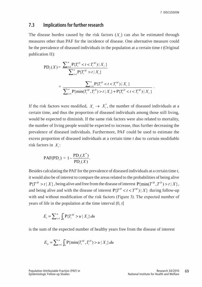
69Research 34/2010National Institute for Health and Welfare
Population Attributable Fraction (PAF) in Epidemiologic Follow-up Studies
7 dIScuSSIoN
7.3 Implications for further research
The disease burden caused by the risk factors ( iX ) can also be estimated through measures other than PAF for the incidence of disease. One alternative measure could be the prevalence of diseased individuals in the population at a certain time t (Original publication II):
PD ( )t X = 1
1
{ ) | }
{ | }
n D Mi i ii
n Mi ii
T t T X
T t X=
=
Ρ < <
Ρ >∑∑
= 1
1
{ ) | }
{min( , ) | } { ) | }
n D Mi i ii
n M D D Mi i i i i ii
T t T X
T T t X T t T X=
=
Ρ < <
Ρ > + Ρ < <∑
∑.
If the risk factors were modified, iX → *iX , the number of diseased individuals at a
certain time, and thus the proportion of diseased individuals among those still living, would be expected to diminish. If the same risk factors were also related to mortality, the number of living people would be expected to increase, thus further decreasing the prevalence of diseased individuals. Furthermore, PAF could be used to estimate the excess proportion of diseased individuals at a certain time t due to certain modifiable risk factors in iX :
PAF(PD )t = *PD ( )1
PD ( )t
t
XX
− .
Besides calculating the PAF for the prevalence of diseased individuals at a certain time t, it would also be of interest to compare the areas related to the probabilities of being alive { | }MT t XΡ > , being alive and free from the disease of interest {min( , ) | }M DT T t XΡ > ,
and being alive and with the disease of interest { ) | }D MT t T XΡ < < during follow-up with and without modification of the risk factors (Figure 3). The expected number of years of life in the population at the time interval (0, t]
1 0{ | }
tn Mt i iiE T u X du
== Ρ >∑ ∫
is the sum of the expected number of healthy years free from the disease of interest
1 1 0{min( , ) | }
tn M Dt i i ii
E T T u X du=
= Ρ >∑ ∫
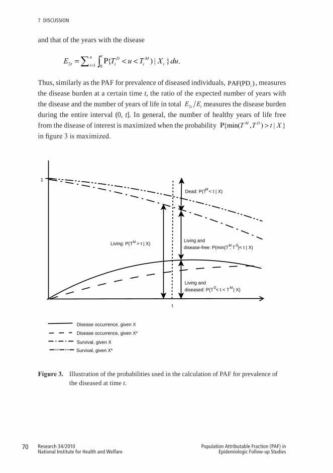
70 Research 34/2010National Institute for Health and Welfare
Population Attributable Fraction (PAF) in Epidemiologic Follow-up Studies
7 dIScuSSIoN
and that of the years with the disease
2 1 0{ ) | }
tn D Mt i i ii
E T u T X du=
= Ρ < <∑ ∫ .
Thus, similarly as the PAF for prevalence of diseased individuals, PAF(PD )t , measures the disease burden at a certain time t, the ratio of the expected number of years with the disease and the number of years of life in total 2t tE E measures the disease burden during the entire interval (0, t]. In general, the number of healthy years of life free from the disease of interest is maximized when the probability {min( , ) | }M DT T t XΡ >in figure 3 is maximized.
t
1
Living: P(T > t | X)M Living anddisease-free: P(min(T , T )< t | X)
Living and diseased: P(T < t < T | X)
Dead: P(T < t | X)M
M D
D M
Disease occurrence, given X
Disease occurrence, given X*
Survival, given X
Survival, given X*
3
Figure3. Illustration of the probabilities used in the calculation of PAF for prevalence of the diseased at time t.
71Research 34/2010National Institute for Health and Welfare
Population Attributable Fraction (PAF) in Epidemiologic Follow-up Studies
7 dIScuSSIoN
The estimation of these measures requires that the follow-up continues after the occurrence of the non-fatal disease so that the risk of death after the occurrence of the disease can be evaluated. It should be taken into account that the risk factors measured at the baseline may, however, no longer predict death after the individual has contracted the disease. Instead, some new risk factors, possibly related to the treatment of the disease, may be more effective predictors of death. Thus, new measurements of such individually relevant risk factors from the time of the occurrence of the disease onwards are needed to guarantee reliable estimates of the risk of death also after having contracted the disease. Since most cohort data sets only include measurements at the baseline, only the effects of average treatment can be evaluated in them. The size of the data is another relevant issue related to the reliable estimation of risk of death after the occurrence of the disease. A sufficient number of disease cases during the entire follow-up from the baseline and, subsequently, a sufficient number of death cases during the follow-up from the disease occurrence until the end of the follow-up are needed to obtain reliable estimates. Furthermore, the amount of time that has passed since the disease occurrence may also affect the risk of death and should also be considered in the model.
So far, in the estimation of PAF the outcome has been assumed to be binary. Extension of the calculation of PAF also for continuous outcomes would be useful, however. Furthermore, although the estimation of PAF has been dealt with in relation to classical epidemiological research designs – cross-sectional, case-control and cohort study designs – the extension of the concept of PAF also for a nested case-control design and a cohort study with repeated measurements is still needed.
72 Research 34/2010National Institute for Health and Welfare
Population Attributable Fraction (PAF) in Epidemiologic Follow-up Studies
8 ConCLUSIonS
This study examined the concept, calculation, programming and application of the Population Attributable Fraction (PAF), which assesses the impact of risk factor modification on mortality or morbidity, in a single and pooled cohort study design.
Point and asymptotic variance estimators of PAF for a certain time interval, based on a parametric piecewise constant hazards model, both for total mortality and disease incidence were developed. In the estimation of PAF for disease incidence, censoring due to death was taken into account. Methods to assess the impact of potential effect modification in the estimation of PAF and for pooling of the PAF estimates in a cohort study design were provided. A new program based on the SAS software for the estimation of PAF, both for mortality and disease incidence, was developed.
This study shed light on the importance of considering the time perspective in the estimation of PAF. A tendency of the PAF estimates, due to various reasons, to decrease in time, and ultimately become meaningless, was demonstrated. This study also showed how ignoring censoring due to death in the estimation of PAF for disease incidence, especially with long follow-up times, leads to an overestimation of the proportion of the disease cases that could be prevented by the risk factor modification in question. Thus, to avoid biased conclusions, censoring due to death should always be considered in the calculation of PAF of morbidity. The new, publicly available program, considering censoring due to death, provided in this study can help to attain this goal, as well as in general to promote the estimation of PAF in cohort studies. As demonstrated in the practical application regarding risk factors of type 2 diabetes, PAF is a very useful public health measure in the evaluation of the relative importance of different, potential risk factors of specific diseases. Pooling of PAF estimates from single cohort studies further increases the power to detect associations.
Extending further the consideration of time perspective in the estimation of PAF, by also taking into account the potential delay from the risk factor modification to the change in the outcome, would be useful with regard to practical applications. Similarly, letting the intended risk factor modification be successful for only a fraction of persons may be more realistic. Also, being able to divide fairly the total PAF obtained for a combination of several risk factors to its components would be useful in the evaluation

73Research 34/2010National Institute for Health and Welfare
Population Attributable Fraction (PAF) in Epidemiologic Follow-up Studies
8 coNcluSIoNS
of the role of single risk factors in different risk factor combinations. Furthermore, to evaluate both the direct and indirect effect of the risk factor modification, the changes it may bring about on the values of other factors should be studied. Finally, it would be useful to extend the concept of PAF to cover different kinds of measures of burden, such as the expected gain in healthy years of life, to be applied in different studies, depending on the size and type of data available for the analysis.

74 Research 34/2010National Institute for Health and Welfare
Population Attributable Fraction (PAF) in Epidemiologic Follow-up Studies
9 ACKnoWLEDGEMEnTS
This study was carried out in the Population Health Unit of the Department of Health, Functional Capacity and Welfare within the Division of Welfare and Health Policies, National Institute for Health and Welfare (THL) in 2006–2010. I am most grateful for the opportunity to work in such a highly professional and inspiring research environment and for the excellent research facilities provided by THL. The data in this study is based on the Mini-Finland Health Survey and Health 2000 Survey and I am indebted for the staff and participants of these surveys for allowing me to work with such high quality datasets. I gratefully acknowledge the financial support from the Doctoral Programs in Public Health for the years 2006–2009 and from the Tampere School of Public Health for finishing my dissertation that has made completion of this study possible.
I feel very privileged to have had the chance to learn from three supervisors, whose expertise, guidance and trust in me throughout this study have been indispensable. My deepest gratitude I wish to express to my principal supervisor Professor Paul Knekt, PHD, who originally came up with the theme for this dissertation and who has been the strongest support for me. His tremendous enthusiasm for scientific research, breadth of knowledge in statistics, epidemiology and health research in general, and great devotion to his students together with his excellent pedagogical skills is something that I am truly thankful for and sincerely admire. I warmly thank Professor Hannu Oja, PhD for his expert supervision and sharing his extensive knowledge especially with regard to statistical theory and methodology needed at different stages of this study. His clear, down-to-earth teaching that I have had the privilege to enjoy since my basic studies helped me in understanding how new methods are to be developed from the start. I am also very grateful to Doctor Tommi Härkänen, PhD for his friendly and supportive supervision as well as valuable advice and concrete help with respect to many different methodological issues. He also introduced me with the idea of taking potential competing risks into account when calculating the Population Attributable Fraction for some event of interest in a longer follow-up, which became one cornerstone of my study. I could not have wished better supervision for my dissertation – thank you all.

75Research 34/2010National Institute for Health and Welfare
Population Attributable Fraction (PAF) in Epidemiologic Follow-up Studies
9 AcKNoWlEdGEMENtS
Carrying out the research related to this dissertation could not have been possible without the help and support of several people and therefore I also express my sincere thanks to:
Senior Systems Analyst Esa Virtala, my co-author and close collaborator in all the substudies, who made extensive contributions to the development of the SAS program which formed an essential part of my study. I am also very thankful for the many valuable advice regarding programming and performing the analyses given by him throughout this study.
Professor Arpo Aromaa, Head of the former Department of Health and Functional Capacity of the National Public Health Institute (KTL), for offering me the opportunity to work at his department, for introducing me to the field of health research, and for giving me perceptive comments as a co-author of one of the substudies.
My colleague and co-author Harri Rissanen who kindly prepared the extensive data for the empirical substudy and helped me in testing of the new SAS program presented in another substudy. I am also deeply thankful for the numerous helpful and friendly advices in computing and data management, as well as in many practical issues throughout the years.
Professor Antti Reunanen and Docent Markku Heliövaara for their collaboration as my co-authors in one substudy. I especially thank Antti for sharing his broad knowledge on type 2 diabetes with me and Markku for giving me valuable advice and comments and always being so encouraging.
Professor Seppo Koskinen for being so helpful and humane Director of the Department of Health, Functional Capacity and Welfare. Sirkka Rinne, Pirkko Alha, Virpi Killström, Ninni Vanhalakka, Mikko Pekkarinen, Talvikki Leinonen and Sari Korhonen at THL for giving their time to advise and assist me in so many things. Your help did not go unnoticed.
Jaakko Nevalainen for testing the new SAS program and commenting the article in which it was presented. Klaus Nordhausen for his quick and thorough responses to all my queries. Leena Nikkari and Hanna Saressalo for helping me with many practical issues and dissertation affairs at the University of Tampere.

76 Research 34/2010National Institute for Health and Welfare
Population Attributable Fraction (PAF) in Epidemiologic Follow-up Studies
9 AcKNoWlEdGEMENtS
The personnel of the THL library for their rapid and endless efforts to provide me with all the material I asked for and the English Centre for revising the English language of all the original publications and the summary part of this dissertation.
The official reviewers of this dissertation, Professor Esa Läärä and Professor Seppo Sarna, for reading the manuscript and providing me with insightful comments and constructive criticism that helped me to further improve the summary of this dissertation.
Riitta Nieminen for skilful layout of the dissertation and for very flexibly co-operation.
All the present and former fellow workers and friends at THL for your never-ending peer and social support, for sharing my coffee and lunch table and all the worries, and for all the laughs. It is because of the warm and stimulating atmosphere created by you that I enjoy coming to work every day. I cannot thank you enough!
My loving family and friends I owe my warmest and sincerest gratitude. I thank with all my heart my parents Eero and Marjatta for raising me independent, for supporting and encouraging me throughout my life and for always being so proud of everything I have done. My three siblings, Marianne, Marjut and Matti, and their families, who despite the distance I always held and feel close to and look up to, I thank for being the support pillar of my life. The circle of caring friends that I am so fortunate to have I thank for all the relaxing and enjoyable moments we have spent together. Special thanks I reserve to my closest friends Liisa, Anne and Minna for their constant emotional support and taking my mind off research every so often. Finally, I thank Jukka whose love has given me strength and energy also to my work – thank you for putting up with my absences and reminding me of the other things important in life. I do not take you all for granted.

77Research 34/2010National Institute for Health and Welfare
Population Attributable Fraction (PAF) in Epidemiologic Follow-up Studies
10 REFEREnCES
Aalen OO. A linear regression model for the analysis of life times. Stat Med 1989;8:907–925.
Alberti KG, Zimmet P, Shaw J. Metabolic syndrome--a new world-wide definition. A Consensus Statement from the International Diabetes Federation. Diabet Med 2006;23:469–480.
Alberti KG, Zimmet P, Shaw J. International Diabetes Federation: a consensus on Type 2 diabetes prevention. Diabet Med 2007;24:451–463.
Alho OP, Läärä E, Oja H. Public health impact of various risk factors for acute otitis media in northern Finland. Am J Epidemiol 1996;143:1149–1156.
Andersen PK, Borgan O, Gill RD, Keiding N. Statistical models based on counting processes. New York: Springer, 1993.
Arjas E, Gasbarra D. Nonparametric bayesian inference from right censored survival data, using the Gibbs sampler. Statistica Sinica 1994;4:505–524.
Aromaa A, Heliövaara M, Impivaara O, Knekt P, Maatela J. Aims, methods and study population. Part 1. In: Aromaa A, Heliövaara M, Impivaara O, Knekt P, Maatela J, eds. The execution of the Mini-Finland Health Survey. (In Finnish, English summary). Helsinki and Turku: Publications of the Social Insurance Institution, Finland, 1989, ML:88.
Aromaa A, Koskinen S, eds. Health and functional capacity in Finland. Baseline results of the Health 2000 health examination. Helsinki: Publications of the National Public Health Institute, 2004, B12.
Basu S, Landis JR. Model-based estimation of population attributable risk under cross-sectional sampling. Am J Epidemiol 1995;142:1338–1343.
Benichou J. Methods of adjustment for estimating the attributable risk in case-control studies: a review. Stat Med 1991;10:1753–1773.
Benichou J. A review of adjusted estimators of attributable risk. Stat Methods Med Res 2001;10:195–216.
Benichou J, Gail MH. A delta-method for implicitly defined random variables. Am Stat 1989;43:41–44.
Benichou J, Gail MH. Variance calculations and confidence intervals for estimates of the attributable risk based on logistic models. Biometrics 1990;46:991–1003.
Bickel PJ, Doksum KA. Mathematical statistics: basic ideas and selected topics. (2nd ed.). Upper Saddle River, NJ: Prentice Hall, 2001.
Brady AR. Adjusted population attributable fractions from logistic regression. Stata Technical Bulletin 1998;7.
78 Research 34/2010National Institute for Health and Welfare
Population Attributable Fraction (PAF) in Epidemiologic Follow-up Studies
10 REFERENcES
Breslow NE. Covariance analysis of censored survival data. Biometrics 1974;30.
Breslow NE, Day NE. Statistical methods in cancer research. Vol. 1: The analysis of case-control studies. Lyon: International Agency for Research on Cancer Scientific Publications, 1980.
Bruzzi P, Green SB, Byar DP, Brinton LA, Schairer C. Estimating the population attributable risk for multiple risk factors using case-control data. Am J Epidemiol 1985;122:904–914.
Cameron AJ, Magliano DJ, Zimmet PZ, Welborn TA, Colagiuri S, Tonkin AM, Shaw JE. The metabolic syndrome as a tool for predicting future diabetes: the AusDiab study. J Intern Med 2008;264:177–186.
Chen YQ, Hu C, Wang Y. Attributable risk function in the proportional hazards model for censored time-to-event. Biostatistics 2006;7:515–529.
Cheung BM, Wat NM, Man YB, Tam S, Thomas GN, Leung GM, Cheng CH, et al. Development of diabetes in Chinese with the metabolic syndrome: a 6-year prospective study. Diabetes Care 2007;30:1430–1436.
Cole P, MacMahon B. Attributable risk percent in case-control studies. Br J Prev Soc Med 1971;25:242–244.
Coughlin SS, Benichou J, Weed DL. Attributable risk estimation in case-control studies. Epidemiol Rev 1994;16:51–64.
Cox C, Chu H, Muñoz A. Survival attributable to an exposure. Stat Med 2009;28:3276–3293.
Cox DR. Regression models and life tables (with discussion). J R Stat Soc B 1972;34:187–220.
Demarqui FN, Loschi RH, Colosimo EA. Estimating the grid of time-points for the piecewise exponential model. Lifetime Data Anal 2008;14:333–356.
DerSimonian R, Laird N. Meta-analysis in clinical trials. Control Clin Trials 1986;7:177–188.
Deubner DC, Tyroler HA, Cassel JC, Hames CG, Becker C. Attributable risk, population attributable risk, and population attributable fraction of death associated with hypertension in a biracial population. Circulation 1975;52:910–918.
Deubner DC, Wilkinson WE, Helms MJ, Tyroler HA, Hames CG. Logistic model estimation of death attributable to risk factors for cardiovascular disease in Evans County, Georgia. Am J Epidemiol 1980;112:135–143.
Drescher K, Becher H. Estimating the generalized impact fraction from case-control data. Biometrics 1997;53:1170–1176.
Eide GE. How to estimate attributable fractions in Stata: A simple introduction. Centre for Clinical Research Research Report. Bergen: Haukeland University Hospital, 2006.
Eide GE, Gefeller O. Sequential and average attributable fractions as aids in the selection of preventive strategies. J Clin Epidemiol 1995;48:645–655.
79Research 34/2010National Institute for Health and Welfare
Population Attributable Fraction (PAF) in Epidemiologic Follow-up Studies
10 REFERENcES
Fleiss JL. Inference about population attributable risk from cross-sectional studies. Am J Epidemiol 1979;110:103–104.
Ford ES, Li C, Sattar N. Metabolic syndrome and incident diabetes: current state of the evidence. Diabetes Care 2008;31:1898–1904.
Friedman M. Piecewise exponential models for survival data with covariates. Ann Statist 1982;10:101–113.
Gail MH, Pfeiffer RM. On criteria for evaluating models of absolute risk. Biostatistics 2005;6:227–239.
Gefeller O. Comparison of adjusted attributable risk estimators. Stat Med 1992;11:2083–2091.
Gefeller O. Definitions of attributable risk--revisited. Public Health Rev 1995;23:343–355.
Greenland S. Variance estimators for attributable fraction estimates consistent in both large strata and sparse data. Stat Med 1987;6:701–708.
Greenland S, Drescher K. Maximum likelihood estimation of the attributable fraction from logistic models. Biometrics 1993;49:865–872.
Greenland S, Robins JM. Conceptual problems in the definition and interpretation of attributable fractions. Am J Epidemiol 1988;128:1185–1197.
Grömping U, Weimann U. The asymptotic distribution of the partial attributable risk in cross-sectional studies. Statistics 2004;38.
Hakulinen T. On competing risks of death. Helsinki: The Finnish Statistical Society, 1977.
Hanson RL, Imperatore G, Bennett PH, Knowler WC. Components of the “metabolic syndrome” and incidence of type 2 diabetes. Diabetes 2002;51:3120–3127.
Heliövaara M, Reunanen A, Aromaa A, Knekt P, Aho K, Suhonen O. Validity of hospital discharge data in a prospective epidemiological study on stroke and myocardial infarction. Acta Med Scand 1984;216:309–315.
Hu FB, Manson JE, Stampfer MJ, Colditz G, Liu S, Solomon CG, Willett WC. Diet, lifestyle, and the risk of type 2 diabetes mellitus in women. N Engl J Med 2001;345:790–797.
Hu G, Lakka TA, Lakka HM, Tuomilehto J. Lifestyle management in the metabolic syndrome. Metab Syndr Relat Disord 2006;4:270–286.
Kahn MJ, O’Fallon WM, Sicks JD. Generalized population attributable risk estimation. Technical Report #54. Rochester, Minnesota: May Foundation, 1998.
Kanaya AM, Wassel Fyr CL, de Rekeneire N, Shorr RI, Schwartz AV, Goodpaster BH, Newman AB, et al. Predicting the development of diabetes in older adults: the derivation and validation of a prediction rule. Diabetes Care 2005;28:404–408.
Kay R, Kinnersley N. On the use of the accelerated failure time model as an alternative to the proportional hazards model in the treatment of time to event data: a case study on influenza. Drug Inf J 2002;36:571–579.

80 Research 34/2010National Institute for Health and Welfare
Population Attributable Fraction (PAF) in Epidemiologic Follow-up Studies
10 REFERENcES
Knekt P, Laaksonen M, Mattila C, Härkänen T, Marniemi J, Heliövaara M, Rissanen H, et al. Serum vitamin D and subsequent occurrence of type 2 diabetes. Epidemiology 2008;19:666–671.
Knekt P, Ritz J, Pereira MA, O’Reilly EJ, Augustsson K, Fraser GE, Goldbourt U, et al. Antioxidant vitamins and coronary heart disease risk: a pooled analysis of 9 cohorts. Am J Clin Nutr 2004;80:1508–1520.
Knowler WC, Barrett-Connor E, Fowler SE, Hamman RF, Lachin JM, Walker EA, Nathan DM. Reduction in the incidence of type 2 diabetes with lifestyle intervention or metformin. N Engl J Med 2002;346:393–403.
Korn EL, Graubard BI, Midthune D. Time-to-event analysis of longitudinal follow-up of a survey: choice of the time-scale. Am J Epidemiol 1997;145:72–80.
Kostner GM. Letter: Enzymatic determination of cholesterol in high-density lipoprotein fractions prepared by polyanion precipitation. Clin Chem 1976;22:695.
Kuritz SJ, Landis JR. Summary attributable risk estimation from unmatched case-control data. Stat Med 1988a;7:507–517.
Kuritz SJ, Landis JR. Attributable risk estimation from matched case-control data. Biometrics 1988b;44:355–367.
Lehnert-Batar A. pARtial: pARtial package. R package Version 0.1., 2006.
Leung HM, Kupper LL. Comparisons of confidence intervals for attributable risk. Biometrics 1981;37:293–302.
Levin ML. The occurrence of lung cancer in man. Acta Unio Int Contra Cancrum 1953;9:531–541.
Leviton A. Letter: Definitions of attributable risk. Am J Epidemiol 1973;98:231.
Liberopoulos EN, Tsouli S, Mikhailidis DP, Elisaf MS. Preventing type 2 diabetes in high risk patients: an overview of lifestyle and pharmacological measures. Curr Drug Targets 2006;7:211–228.
Lim HJ, Zhang X. Semi-parametric additive risk models: application to injury duration study. Accid Anal Prev 2009;41:211–216.
Lin DY. On the Breslow estimator. Lifetime Data Anal 2007;13:471–480.
Lindstrom J, Tuomilehto J. The diabetes risk score: a practical tool to predict type 2 diabetes risk. Diabetes Care 2003;26:725–731.
Lumley T, Kronmal R, Shuangge M. Relative risk regression in medical research: models, contrasts, estimators, and algorithms. In: UW Biostatistics, Working Paper Series, Paper 293. University of Washington: The Berkeley Electronic Press, 2006.
MacMahon B, Pugh TF. Epidemiology; principles and methods. Boston: Little, 1970.
81Research 34/2010National Institute for Health and Welfare
Population Attributable Fraction (PAF) in Epidemiologic Follow-up Studies
10 REFERENcES
McNeely MJ, Boyko EJ, Leonetti DL, Kahn SE, Fujimoto WY. Comparison of a clinical model, the oral glucose tolerance test, and fasting glucose for prediction of type 2 diabetes risk in Japanese Americans. Diabetes Care 2003;26:758–763.
Mezzetti M, Ferraroni M, Decarli A, La Vecchia C, Benichou J. Software for attributable risk and confidence interval estimation in case-control studies. Comput Biomed Res 1996;29:63–75.
Miettinen OS. Proportion of disease caused or prevented by a given exposure, trait or intervention. Am J Epidemiol 1974;99:325–332.
Morgenstern H, Bursic ES. A method for using epidemiologic data to estimate the potential impact of an intervention on the health status of a target population. J Community Health 1982;7:292–309.
Mozaffarian D, Kamineni A, Carnethon M, Djoussé L, Mukamal KJ, Siskovick D. Lifestyle factors and new-onset diabetes mellitus in older adults. Arch Intern Med 2009;169: 798–807.
Narayan KM, Kanaya AM, Gregg EW. Lifestyle intervention for the prevention of type 2 diabetes mellitus: putting theory to practice. Treat Endocrinol 2003;2:315–320.
Norberg M, Eriksson JW, Lindahl B, Andersson C, Rolandsson O, Stenlund H, Weinehall L. A combination of HbA1c, fasting glucose and BMI is effective in screening for individuals at risk of future type 2 diabetes: OGTT is not needed. J Intern Med 2006;260:263–271.
Oja H, Alho OP, Läärä E. Model-based estimation of the excess fraction (attributable fraction): day care and middle ear infection. Stat Med 1996;15:1519–1534.
Olsen CM, Carroll HJ, Whiteman DC. Familial melanoma: a meta-analysis and estimates of attributable fraction. Cancer Epidemiol Biomarkers Prev 2010;19:65–73.
Orchard TJ, Temprosa M, Goldberg R, Haffner S, Ratner R, Marcovina S, Fowler S. The effect of metformin and intensive lifestyle intervention on the metabolic syndrome: the Diabetes Prevention Program randomized trial. Ann Intern Med 2005;142:611–619.
Ouellet BL, Romeder JM, Lance JM. Premature mortality attributable to smoking and hazardous drinking in Canada. Am J Epidemiol 1979;109:451–463.
Pichlmeier U, Gefeller O. Conceptual aspects of attributable risk with recurrent disease events. Stat Med 1997;16:1107–1120.
Pittas AG, Dawson-Hughes B, Li T, Van Dam RM, Willett WC, Manson JE, Hu FB. Vitamin D and calcium intake in relation to type 2 diabetes in women. Diabetes Care 2006;29:650–656.
Rabe C, Lehnert-Batar A, Gefeller O. Generalized approaches to partitioning the attributable risk of interacting risk factors can remedy existing pitfalls. J Clin Epidemiol 2007;60:461–468.
Reunanen A, Aromaa A, Pyörälä K, Punsar S, Maatela J, Knekt P. The Social Insurance Institution’s coronary heart disease study. Baseline data and 5-year mortality experience. Acta Med Scand Suppl 1983;673:1–120.

82 Research 34/2010National Institute for Health and Welfare
Population Attributable Fraction (PAF) in Epidemiologic Follow-up Studies
10 REFERENcES
Reunanen A, Kangas T, Martikainen J, Klaukka T. Nationwide survey of comorbidity, use, and costs of all medications in Finnish diabetic individuals. Diabetes Care 2000;23:1265–1271.
Rockhill B, Newman B, Weinberg C. Use and misuse of population attributable fractions. Am J Public Health 1998;88:15–19.
Rothman KJ, Greenland S, Lash TL. Modern epidemiology. (3rd ed.). Philadelpia, PA: Lippincott Williams & Wilkins, 2008.
Rückinger S, von Kries R, Toschke AM. An illustration and programs for estimating attributable fraction in large scale surveys considering multiple risk factors. Comput Methods Programs Biomed 2009.
Rämsch C, Pfahlberg AB, Gefeller O. Point and interval estimation of partial attributable risks from case-control data using the R-package ‘pARccs’. Comput Methods Programs Biomed 2009;94:88–95.
Samuelsen SO, Eide GE. Attributable fractions with survival data. Stat Med 2008;27:1447–1467.
SAS Institute Inc. SAS/STAT User’s Guide, Version 9.1. Cary, NC: SAS Institute Inc, 2007.
Schmidt MI, Duncan BB, Bang H, Pankow JS, Ballantyne CM, Golden SH, Folsom AR, et al. Identifying individuals at high risk for diabetes: The Atherosclerosis Risk in Communities study. Diabetes Care 2005;28:2013–2018.
Schulze MB, Hoffmann K, Boeing H, Linseisen J, Rohrmann S, Mohlig M, Pfeiffer AF, et al. An accurate risk score based on anthropometric, dietary, and lifestyle factors to predict the development of type 2 diabetes. Diabetes Care 2007;30:510–515.
Schulze MB, Hu FB. Primary prevention of diabetes: what can be done and how much can be prevented? Annu Rev Public Health 2005;26:445–467.
Schumacher M, Wangler M, Wolkewitz M, Beyersmann J. Attributable mortality due to nosocomial infections. A simple and useful application of multistate models. Methods Inf Med 2007;46:595–600.
Silverberg MJ, Smith MW, Chmiel JS, Detels R, Margolick JB, Rinaldo CR, O’Brien SJ, et al. Fraction of cases of acquired immunodeficiency syndrome prevented by the interactions of identified restriction gene variants. Am J Epidemiol 2004;159:232–241.
Smith-Warner SA, Spiegelman D, Ritz J, Albanes D, Beeson WL, Bernstein L, Berrino F, et al. Methods for pooling results of epidemiologic studies: the Pooling Project of Prospective Studies of Diet and Cancer. Am J Epidemiol 2006;163:1053–1064.
Spiegelman D, Hertzmark E, Wand HC. Point and interval estimates of partial population attributable risks in cohort studies: examples and software. Cancer Causes Control 2007;18:571–579.
Stern MP, Williams K, Haffner SM. Identification of persons at high risk for type 2 diabetes mellitus: do we need the oral glucose tolerance test? Ann Intern Med 2002;136:575–581.
83Research 34/2010National Institute for Health and Welfare
Population Attributable Fraction (PAF) in Epidemiologic Follow-up Studies
10 REFERENcES
Stram DO. Meta-analysis of published data using a linear mixed-effects model. Biometrics 1996;52:536–544.
Sturmans F, Mulder PG, Valkenburg HA. Estimation of the possible effect of interventive measures in the area of ischemic heart diseases by the attributable risk percentage. Am J Epidemiol 1977;105:281–289.
Taslim S, Tai ES. The relevance of the metabolic syndrome. Ann Acad Med Singapore 2009;38:29–33.
Therneau TM, Grambsch PM. Modeling survival data: extending the Cox model: Springer, 2000.
Uter W, Pfahlberg A. The concept of attributable risk in epidemiological practice. Biom J 1999;41:985–999.
Uter W, Pfahlberg A. The application of methods to quantify attributable risk in medical practice. Stat Methods Med Res 2001;10:231–237.
Walter SD. The distribution of Levin’s measure of attributable risk. Biometrika 1975;62:371–374.
Walter SD. The estimation and interpretation of attributable risk in health research. Biometrics 1976;32:829–849.
Walter SD. Prevention for multifactorial diseases. Am J Epidemiol 1980;112:409–416.
van Dam RM. The epidemiology of lifestyle and risk for type 2 diabetes. Eur J Epidemiol 2003;18:1115–1125.
Whittemore AS. Statistical methods for estimating attributable risk from retrospective data. Stat Med 1982;1:229–243.
Whittemore AS. Estimating attributable risk from case-control studies. Am J Epidemiol 1983;117:76–85.
Wild S, Roglic G, Green A, Sicree R, King H. Global prevalence of diabetes: estimates for the year 2000 and projections for 2030. Diabetes Care 2004;27:1047–1053.
World Health Organization. Diabetes Mellitus: Report of a WHO study group. Geneva, 1985.

84 Research 34/2010National Institute for Health and Welfare
Population Attributable Fraction (PAF) in Epidemiologic Follow-up Studies
APPEnDICESAPPENDICES
Appendix 1. Sample SAS code for calculating PAF for total mortality with piecewise
constant hazards model
The SAS program for the estimation of PAF for total mortality and its 95% confidence
interval requires the SAS procedures LIFEREG and IML and the following inputs:
DES = Design matrix (n*J rows and B+J+B*J+m columns) for baseline hazard
parameters and observed covariates, which indicates the categories of the baseline
hazard variables (follow-up time intervals, birth cohorts, and their interactions) that
each individual belongs to at each follow-up time interval and which values of the risk
factors each individual has.
DES_STAR = Design matrix (n*J rows and B+J+B*J+m columns) for baseline
hazard parameters and modified covariates, which indicates the categories of the
baseline hazard variables (follow-up time intervals, birth cohorts, and their
interactions) that each individual belongs to at each follow-up time interval and which
values of the risk factor each individual has after the hypothetical change of the risk
factors of interest.
EST = Column vector (B+J+B*J+m rows) of parameter estimates for the baseline
hazard variables and the risk factors obtained from the LIFEREG analysis.
COVB = Covariance matrix (B+J+B*J+m rows and columns) of the parameter
estimates for the baseline hazard variables and the risk factors obtained from the
LIFEREG analysis.
To estimate PAF for a chosen time interval ( , ]t t t+ Δ , the user must define the
exposure at different time intervals until time t (DELTA_1) and time
t t+ Δ (DELTA_2). For example, to estimate PAF for total mortality for a time interval
(0, 20] when the follow-up time is divided into four 5-year time intervals, the user
must define:
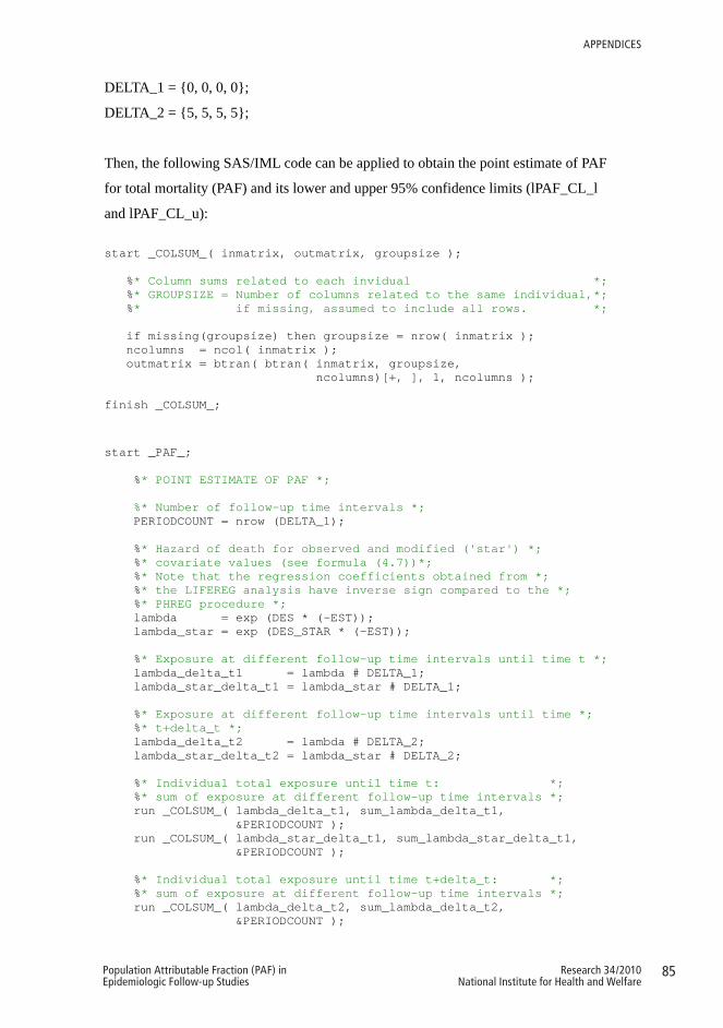
85Research 34/2010National Institute for Health and Welfare
Population Attributable Fraction (PAF) in Epidemiologic Follow-up Studies
APPENdIcES
DELTA_1 = {0, 0, 0, 0};
DELTA_2 = {5, 5, 5, 5};
Then, the following SAS/IML code can be applied to obtain the point estimate of PAF
for total mortality (PAF) and its lower and upper 95% confidence limits (lPAF_CL_l
and lPAF_CL_u): start _COLSUM_( inmatrix, outmatrix, groupsize ); %* Column sums related to each invidual *; %* GROUPSIZE = Number of columns related to the same individual,*; %* if missing, assumed to include all rows. *; if missing(groupsize) then groupsize = nrow( inmatrix ); ncolumns = ncol( inmatrix ); outmatrix = btran( btran( inmatrix, groupsize, ncolumns)[+, ], 1, ncolumns ); finish _COLSUM_;
start _PAF_; %* POINT ESTIMATE OF PAF *; %* Number of follow-up time intervals *;
PERIODCOUNT = nrow (DELTA_1);
%* Hazard of death for observed and modified ('star') *; %* covariate values (see formula (4.7))*; %* Note that the regression coefficients obtained from *; %* the LIFEREG analysis have inverse sign compared to the *; %* PHREG procedure *;
lambda = exp (DES * (-EST)); lambda_star = exp (DES_STAR * (-EST)); %* Exposure at different follow-up time intervals until time t *; lambda_delta_t1 = lambda # DELTA_1; lambda_star_delta_t1 = lambda_star # DELTA_1;
%* Exposure at different follow-up time intervals until time *; %* t+delta_t *;
lambda_delta_t2 = lambda # DELTA_2; lambda_star_delta_t2 = lambda_star # DELTA_2; %* Individual total exposure until time t: *; %* sum of exposure at different follow-up time intervals *;
run _COLSUM_( lambda_delta_t1, sum_lambda_delta_t1, &PERIODCOUNT ); run _COLSUM_( lambda_star_delta_t1, sum_lambda_star_delta_t1, &PERIODCOUNT );
%* Individual total exposure until time t+delta_t: *; %* sum of exposure at different follow-up time intervals *;
run _COLSUM_( lambda_delta_t2, sum_lambda_delta_t2, &PERIODCOUNT );
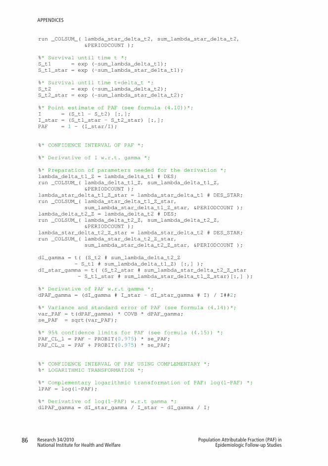
86 Research 34/2010National Institute for Health and Welfare
Population Attributable Fraction (PAF) in Epidemiologic Follow-up Studies
APPENdIcES
run _COLSUM_( lambda_star_delta_t2, sum_lambda_star_delta_t2, &PERIODCOUNT );
%* Survival until time t *; S_t1 = exp (-sum_lambda_delta_t1); S_t1_star = exp (-sum_lambda_star_delta_t1); %* Survival until time t+delta_t *; S_t2 = exp (-sum_lambda_delta_t2); S_t2_star = exp (-sum_lambda_star_delta_t2); %* Point estimate of PAF (see formula (4.10))*; I = (S_t1 - S_t2) [:,]; I_star = (S_t1_star - S_t2_star) [:,]; PAF = 1 - (I_star/I); %* CONFIDENCE INTERVAL OF PAF *; %* Derivative of I w.r.t. gamma *; %* Preparation of parameters needed for the derivation *; lambda_delta_t1_Z = lambda_delta_t1 # DES;
run _COLSUM_( lambda_delta_t1_Z, sum_lambda_delta_t1_Z, &PERIODCOUNT );
lambda_star_delta_t1_Z_star = lambda_star_delta_t1 # DES_STAR; run _COLSUM_( lambda_star_delta_t1_Z_star, sum_lambda_star_delta_t1_Z_star, &PERIODCOUNT );
lambda_delta_t2_Z = lambda_delta_t2 # DES; run _COLSUM_( lambda_delta_t2_Z, sum_lambda_delta_t2_Z, &PERIODCOUNT );
lambda_star_delta_t2_Z_star = lambda_star_delta_t2 # DES_STAR; run _COLSUM_( lambda_star_delta_t2_Z_star, sum_lambda_star_delta_t2_Z_star, &PERIODCOUNT );
dI_gamma = t( (S_t2 # sum_lambda_delta_t2_Z - S_t1 # sum_lambda_delta_t1_Z) [:,] ); dI_star_gamma = t( (S_t2_star # sum_lambda_star_delta_t2_Z_star - S_t1_star # sum_lambda_star_delta_t1_Z_star)[:,] ); %* Derivative of PAF w.r.t gamma *; dPAF_gamma = (dI_gamma # I_star - dI_star_gamma # I) / I##2; %* Variance and standard error of PAF (see formula (4.14))*; var_PAF = t(dPAF_gamma) * COVB * dPAF_gamma; se_PAF = sqrt(var_PAF); %* 95% confidence limits for PAF (see formula (4.15)) *; PAF_CL_l = PAF - PROBIT(0.975) * se_PAF; PAF_CL_u = PAF + PROBIT(0.975) * se_PAF;
%* CONFIDENCE INTERVAL OF PAF USING COMPLEMENTARY *; %* LOGARITHMIC TRANSFORMATION *;
%* Complementary logarithmic transformation of PAF: log(1-PAF) *; lPAF = log(1-PAF); %* Derivative of log(1-PAF) w.r.t gamma *; dlPAF_gamma = dI_star_gamma / I_star - dI_gamma / I;

87Research 34/2010National Institute for Health and Welfare
Population Attributable Fraction (PAF) in Epidemiologic Follow-up Studies
APPENdIcES
%* Variance and standard error of log(1-PAF) *; var_lPAF = t(dlPAF_gamma) * COVB * dlPAF_gamma; se_lPAF = sqrt(var_lPAF);
%* 95% confidence limits for inverse log(1-PAF) (see formula *; %* (4.16)) *;
lPAF_CL_l = 1 - exp(lPAF + PROBIT(0.975) * se_lPAF); lPAF_CL_u = 1 - exp(lPAF - PROBIT(0.975) * se_lPAF); finish _PAF_;
88 Research 34/2010National Institute for Health and Welfare
Population Attributable Fraction (PAF) in Epidemiologic Follow-up Studies
APPENdIcES
Appendix 2. Sample SAS code for calculating PAF for disease incidence with
piecewise constant hazards model
The SAS program for the estimation of PAF for disease incidence and its 95%
confidence interval requires the SAS procedures LIFEREG and IML and the
following inputs:
DES = Design matrix (n*J rows and B+J+B*J+m columns) for baseline hazard
parameters and observed covariates, which indicates the categories of the baseline
hazard variables (follow-up time intervals, birth cohorts, and their interactions) that
each individual belongs to at each follow-up time interval and which values of the risk
factors each individual has.
DES_STAR = Design matrix (n*J rows and B+J+B*J+m columns) for baseline
hazard parameters and modified covariates, which indicates the categories of the
baseline hazard variables (follow-up time intervals, birth cohorts, and their
interactions) that each individual belongs to at each follow-up time interval and which
values of the risk factor each individual has after the hypothetical change of the risk
factors of interest.
EST_M = Column vector (B+J+B*J+m rows) of parameter estimates for the baseline
hazard variables and the risk factors related to mortality obtained from the LIFEREG
analysis.
EST_D = Column vector (B+J+B*J+m rows) of parameter estimates for the baseline
hazard variables and the risk factors related to disease incidence obtained from the
LIFEREG analysis.
COVB_M = Covariance matrix (B+J+B*J+m rows and columns) of the parameter
estimates for the baseline hazard variables and the risk factors related to mortality
obtained from the LIFEREG analysis.
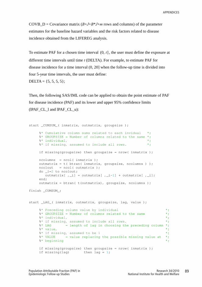
89Research 34/2010National Institute for Health and Welfare
Population Attributable Fraction (PAF) in Epidemiologic Follow-up Studies
APPENdIcES
COVB_D = Covariance matrix (B+J+B*J+m rows and columns) of the parameter
estimates for the baseline hazard variables and the risk factors related to disease
incidence obtained from the LIFEREG analysis.
To estimate PAF for a chosen time interval (0, ]t , the user must define the exposure at
different time intervals until time t (DELTA). For example, to estimate PAF for
disease incidence for a time interval (0, 20] when the follow-up time is divided into
four 5-year time intervals, the user must define:
DELTA = {5, 5, 5, 5};
Then, the following SAS/IML code can be applied to obtain the point estimate of PAF
for disease incidence (PAF) and its lower and upper 95% confidence limits
(lPAF_CL_l and lPAF_CL_u):
start _CUMSUM_( inmatrix, outmatrix, groupsize ); %* Cumulative column sums related to each invidual *; %* GROUPSIZE = Number of columns related to the same *; %* individual, *; %* if missing, assumed to include all rows. *; if missing(groupsize) then groupsize = nrow( inmatrix ); ncolumns = ncol( inmatrix ); outmatrix = t( btran( inmatrix, groupsize, ncolumns ) ); ncolout = ncol( outmatrix ); do _i=2 to ncolout; outmatrix[ ,_i] = outmatrix[ ,_i-1] + outmatrix[ ,_i]; end; outmatrix = btran( t(outmatrix), groupsize, ncolumns ); finish _CUMSUM_; start _LAG_( inmatrix, outmatrix, groupsize, lag, value ); %* Preceding column value by individual *; %* GROUPSIZE = Number of columns related to the same *; %* individual, *; %* if missing, assumed to include all rows. *; %* LAG = length of lag in choosing the preceding column *; %* value, *; %* if missing, assumed to be 1 *; %* VALUE = value replacing the possible missing value at *; %* beginning *; if missing(groupsize) then groupsize = nrow( inmatrix ); if missing(lag) then lag = 1;

90 Research 34/2010National Institute for Health and Welfare
Population Attributable Fraction (PAF) in Epidemiologic Follow-up Studies
APPENdIcES
if groupsize<=1 then outmatrix = j( nrow(inmatrix), ncol(inmatrix), value ); else do; ncolumns = ncol( inmatrix ); outmatrix = t( btran( inmatrix, groupsize, ncolumns ) ); nrowout = nrow( outmatrix ); outmatrix = btran( t( j(nrowout, lag, value) || outmatrix[ ,1:groupsize-lag] ), groupsize, ncolumns ); end; finish _LAG_; start _PAF_; %* POINT ESTIMATE OF PAF *; %* Number of follow-up time intervals *;
PERIODCOUNT = nrow (DELTA);
%* Hazard of death for observed and modified ('star') *; %* covariate values (see formula (4.7))*;
%* Note that the regression coefficients obtained from *; %* the LIFEREG analysis have inverse sign compared to the *; %* PHREG procedure *;
lambda_M = exp (DES * (-EST_M)); lambda_M_star = exp (DES_STAR * (-EST_M));
%* Hazard of disease incidence for observed and modified *; %* ('star') covariate values (see formula (4.8))*;
lambda_D = exp (DES * (-EST_D)); lambda_D_star = exp (DES_STAR * (-EST_D)); %* Sum of hazard of death and hazard of disease incidence *; lambda_M_plus_D = lambda_M + lambda_D; lambda_M_plus_D_star = lambda_M_star + lambda_D_star; %* Probability that the observed event is disease *; dis_prob = lambda_D / lambda_M_plus_D; dis_prob_star = lambda_D_star / lambda_M_plus_D_star;
%* Exposure at different follow-up time intervals until the *; %* end of follow-up *;
lambda_M_plus_D_delta = lambda_M_plus_D # DELTA; lambda_M_plus_D_star_delta = lambda_M_plus_D_star # DELTA;
%* Individual total exposure by the end of each follow-up *; %* time-interval: *;
%* sum of exposure at previous follow-up time intervals *; run _CUMSUM_( lambda_M_plus_D_delta, cs_lambda_M_plus_D_delta, &PERIODCOUNT ); run _CUMSUM_( lambda_M_plus_D_star_delta, cs_lambda_M_plus_D_star_delta, &PERIODCOUNT ); %* Survival until time a_j: S_j ja S_j* *; S_t2 = exp (-cs_lambda_M_plus_D_delta); S_t2_star = exp (-cs_lambda_M_plus_D_star_delta);
%* Survival until time a_j-1: S_j-1 ja S_j-1* (calculated *; %* with the help of S_j ja S_j*) *;
run _LAG_( S_t2, S_t1, &PERIODCOUNT, 1, 1 );
91Research 34/2010National Institute for Health and Welfare
Population Attributable Fraction (PAF) in Epidemiologic Follow-up Studies
APPENdIcES
run _LAG_( S_t2_star, S_t1_star, &PERIODCOUNT, 1, 1 ); %* Point estimate of PAF (see formula (4.11))*; I = ( dis_prob # (S_t1 - S_t2) )[:,]; I_star = ( dis_prob_star # (S_t1_star - S_t2_star) )[:,]; PAF = 1 - (I_star/I); %* CONFIDENCE INTERVAL OF PAF *; %* Derivative of I w.r.t. gamma_M *;
%* Preparation of parameters related to mortality needed for *; %* the derivation *;
lambda_M_delta_t2_Z = (lambda_M # DELTA) # DES; run _CUMSUM_( lambda_M_delta_t2_Z, cs_lambda_M_delta_t2_Z, &PERIODCOUNT ); lambda_M_star_delta_t2_Z_star = (lambda_M_star # DELTA) # DES_STAR; run _CUMSUM_( lambda_M_star_delta_t2_Z_star, cs_lambda_M_star_delta_t2_Z_star, &PERIODCOUNT ); run _LAG_( cs_lambda_M_delta_t2_Z, cs_lambda_M_delta_t1_Z, &PERIODCOUNT, 1, 0 ); run _LAG_( cs_lambda_M_star_delta_t2_Z_star, cs_lambda_M_star_delta_t1_Z_star, &PERIODCOUNT, 1, 0 ); dI_gamma_M = ( -DES # lambda_D # lambda_M / (lambda_M_plus_D##2) # (S_t1 - S_t2) + dis_prob # ( S_t2 # cs_lambda_M_delta_t2_Z - S_t1 # cs_lambda_M_delta_t1_Z ) ) [:,]; dI_star_gamma_M = ( -DES_STAR # lambda_D_star # lambda_M_star / (lambda_M_plus_D_star##2) # (S_t1_star - S_t2_star) + dis_prob_star # ( S_t2_star # cs_lambda_M_star_delta_t2_Z_star - S_t1_star # cs_lambda_M_star_delta_t1_Z_star ) ) [:,]; %* Derivative of I w.r.t. gamma_D *;
%* Preparation of parameters related to disease needed for *; %* the derivation *;
lambda_D_delta_t2_Z = (lambda_D # DELTA) # DES; run _CUMSUM_( lambda_D_delta_t2_Z, cs_lambda_D_delta_t2_Z, &PERIODCOUNT ); lambda_D_star_delta_t2_Z_star = (lambda_D_star # DELTA) # DES_STAR; run _CUMSUM_( lambda_D_star_delta_t2_Z_star, cs_lambda_D_star_delta_t2_Z_star, &PERIODCOUNT ); run _LAG_( cs_lambda_D_delta_t2_Z, cs_lambda_D_delta_t1_Z, &PERIODCOUNT, 1, 0 ); run _LAG_( cs_lambda_D_star_delta_t2_Z_star, cs_lambda_D_star_delta_t1_Z_star, &PERIODCOUNT, 1, 0 ); dI_gamma_D = ( DES # lambda_D # lambda_M / (lambda_M_plus_D##2) # (S_t1 - S_t2) + dis_prob # ( S_t2 # cs_lambda_D_delta_t2_Z - S_t1 # cs_lambda_D_delta_t1_Z ) ) [:,]; dI_star_gamma_D = ( DES_STAR # lambda_D_star # lambda_M_star /
92 Research 34/2010National Institute for Health and Welfare
Population Attributable Fraction (PAF) in Epidemiologic Follow-up Studies
APPENdIcES
(lambda_M_plus_D_star##2) # (S_t1_star - S_t2_star) + dis_prob_star # ( S_t2_star # cs_lambda_D_star_delta_t2_Z_star - S_t1_star # cs_lambda_D_star_delta_t1_Z_star ) ) [:,]; %* Derivative of PAF w.r.t. gamma_M *; dPAF_gamma_M = (dI_gamma_M # I_star - dI_star_gamma_M # I) / I##2; %* Derivative of PAF w.r.t. gamma_D *; dPAF_gamma_D = (dI_gamma_D # I_star - dI_star_gamma_D # I) / I##2; %* Variance and standard error of PAF (see formula (4.17)) *; var_PAF = dPAF_gamma_D * COVB_D * t(dPAF_gamma_D) + dPAF_gamma_M * COVB_M * t(dPAF_gamma_M); se_PAF = sqrt(var_PAF); %* 95% confidence limits for PAF (see formula (4.18))*; PAF_CL_l = PAF - PROBIT(0.975) * se_PAF; PAF_CL_u = PAF + PROBIT(0.975) * se_PAF;
%* CONFIDENCE INTERVAL OF PAF USING COMPLEMENTARY *; %* LOGARITHMIC TRANSFORMATION *;
%* Complementary logarithmic transformation of PAF: log(1-PAF)*; lPAF = log(1-PAF); %* Derivative of log(1-PAF) w.r.t gamma_M *; dlPAF_gamma_M = dI_star_gamma_M / I_star - dI_gamma_M / I; %* Derivative of log(1-PAF) w.r.t gamma_D *; dlPAF_gamma_D = dI_star_gamma_D / I_star - dI_gamma_D / I; %* Variance and standard error of log(1-PAF) *; var_lPAF = dlPAF_gamma_D * COVB_D * t(dlPAF_gamma_D) + dlPAF_gamma_M * COVB_M * t(dlPAF_gamma_M); se_lPAF = sqrt(var_lPAF); %* 95% confidence limits for inverse log(1-PAF) (see formula *; %* (4.16))*; lPAF_CL_l = 1 - exp(lPAF + PROBIT(0.975) * se_lPAF); lPAF_CL_u = 1 - exp(lPAF - PROBIT(0.975) * se_lPAF); finish _PAF_;