EHES Manual - Julkari

Part C. EuroPEan lEvEl Collaboration

2nd edition

Hanna Tolonen (editor)

EHES Manual

Directions 2016_15

Edited by

Hanna tolonen

EHES ManualPart C.

European level collaboration

Helsinki 2016

Directions 2016_15

The EHES has received funding from the European Commission/DG Santé (the EHES Pilot Project (2009-2012) and BRIDGE Health Project (2015-2017)).

The views expressed here are those of the authors and they do not represent the Commission’s official posi-tion.

layout: Hanna Tolonen

Cover: Hanna Tolonen

Graphics:

Chapter 2: Ari Haukijärvi

Copyright National Institute for Health and Welfare (THL), Finland and authors

Publisher National Institute for Health and Welfare

PO Box 30, FI-00271 Helsinki, FINLAND

http://www.thl.fi

iSbn (pdf) 978-952-302-702-2

iSSn (pdf) 2323-4172

http://urn.fi/URN:ISBN:978-952-302-702-2

Helsinki, Finland 2016

reference:

Tolonen H (Ed.) EHES Manual. Part C. European level collabo-ratoin. 2nd edition. National Institute for Health and Welfare. 2016. Directions 2016_15. URN:ISBN:978-952-302-702-2 URL: http://urn.fi/URN:ISBN:978-952-302-702-2

ContentsIntroduction 1References 1

1. Data sharing rules 3 1.1 Draft principles and rules for sharing and use of the EHES data for future use 3 1.1.1 Introduction 4 1.1.2 General statement 4 1.1.3 Scope of the data sharing policy - EHES Data 4 1.1.4 Ownership of and obligation to share the data 5 1.1.5 Data Security and Confidentiality 5 1.1.6 Publication policy 6 1.1.6.1 Data assessment and basic reporting 6 1.1.6.2 Additional analysis and research using the data 7 1.1.7 Sharing data with research groups 8 1.1.8 Coordination and decision making 9 1.2 Draft template for EHES Data Transfer Agreement for future use 10 1.3 Principles and rules for sharing and use of the EHES Pilot Project data 12 1.3.1 Introduction 13 1.3.2 General statement 13 1.3.3 Scope of the data sharing policy - EHES Data 13 1.3.4 Ownership of and obligation to share the data 14 1.3.5 Data Security and Confidentiality 14 1.3.6 Publication policy 15 1.3.6.1 Data assessment and basic reporting 15 1.3.6.2 Additional analysis and research using the data 16 1.3.7. Sharing data with research groups 17 1.3.8 Coordination and decision making 18 1.4 Template for EHES Data Transfer Agreement for use in the EHES Pilot Project 18

2. EHES RC data management 21 2.1 Overview 21 2.1.1 Main areas and use cases 21 2.1.2 RC data management system 22 2.1.2.1 Databases 22 2.1.2.2 Applications 22 2.1.2.2.1 Web applications 22 2.1.2.2.2 Other applications 23 2.2 Survey procedures web questionnaire 23

2.3 Transferring survey data to the RC 24 2.3.1 Format of data transfer 25 2.3.2 Data checking 25 2.3.3 Uploading data files to the RC 26 2.4 Survey database 26 2.5 Derived variables and QA 26 Appendix 2a. Data transfer format - Sampling 27 Specification of data items 27 Stage 1 27 Stage 2 30 General instructions and examples 33 Appendix 2b. Data transfer format - Eligibility and participation 37 Specification of data items 37 General instructions 41 Appendix 2c. Data transfer format - Questionnaire data 43 Specification of data items 43 General instructions 50 Appendix 2d. Data transfer format - Measurements data 52 Specification of data items 52 General instructions 59 Appendix 2e. Data transfer format - Laboratory data 60 Specification of data items 60 General instructions 65 Appendix 2f. FAQ of the data transfer 66 Appendix 2g. Survey database scheme 68 Tables 68 Views 70 Functions 70 Procedures 71 Appendix 2h. Tables for the derived variables and QA data 73 A. Tables for the derived variables 73 B. Tables for the QA data 74

3. Evaluation and quality assurance 77 3.1 National level evaluation 77 3.2 European level evaluation 78 3.2.1 Site visits 78 3.2.2 Evaluation of the national manuals 79 3.2.3 Quality assessment of the survey data 80 References 81 Appendix 3a. Template for the national evaluation report 82 Appendix 3b. Contents of the site visits 89 Appendix 3c. National HES manual evaluation template 92 Appendix 3d. Program codes for quality assessment 102 R functions for quality assessment of the survey data 102

4. Indicators 131 4.1 Definition of indicators 131 4.1.1 Blood pressure 131 4.1.1.1 Systolic blood pressure (mmHg) 131 4.1.1.2 Diastolic blood pressure (mmHg) 131 4.1.1.3 Hypertension and categories of blood pressure 132 4.1.1.4 Awareness of elevated blood pressure 133 4.1.1.5 Anti-hypertensive drug use 133 4.1.1.6 Blood pressure measurement 134 4.1.1.7 Pulse rate (beats/min) 134 4.1.2 Lipids 134 4.1.2.1 Serum total cholesterol (mmol/l) 134 4.1.2.2 Serum high-density lipoprotein (HDL) cholesterol (mmol/l) 134 4.1.2.3 Serum non-HDL cholesterol (mmol/l) 135 4.1.2.4 Serum total cholesterol to HDL cholesterol ratio 135 4.1.2.5 Categories of cholesterol level 135 4.1.2.6 Awareness of elevated total cholesterol 137 4.1.2.7 Lipid lowering drug use 137 4.1.2.8 Cholesterol measurement 137 4.1.3 Glucose 138 4.1.3.1 Fasting plasma glucose 138 4.1.3.2 Glycated haemoglobin (HbA1c) 138 4.1.3.3 Diabetes and impaired fasting glucose 138 4.1.3.4 Use of diabetes medication 139 4.1.3.5 Awareness of diabetes 140 4.1.3.6 Glucose measurement 140 4.1.4 Anthropometrics and obesity 140 4.1.4.1 Height (measured) 140 4.1.4.2 Height (self-reported) 141 4.1.4.3 Difference between measured and self- reported height 141 4.1.4.4 Weight (measured) 141 4.1.4.5 Weight (self-reported) 141 4.1.4.6 Difference between measured and self- reported weight 142 4.1.4.7 Waist circumference 142 4.1.4.8 BMI (Based on measured height and weight) 142 4.1.4.9 BMI (based on self-reported height and weight) 143 4.1.4.10 Difference between measured and self-reported BMI 143 4.1.4.11 Obesity and other BMI categories 143

4.1.4.12 Distribution of categories of waist circumference 144 4.1.5 Self-perceived health and other self-reported chronic diseases 145 4.1.6 Smoking 145 4.2 Background variables 147 4.2.1 Socio-economic 148 References 150

5. Reporting 151 5.1 Outline of the basic report 151 5.2 Reporting system 151 5.3 Estimation of indicators 152 5.3.1 Introduction 152 5.3.2 Weighting 152 5.3.3 Estimation 153 5.3.4 Imputation 154 5.3.5 Smoothing 156 5.3.6 Density estimation 157 References 158 Appendix 5a. Template of the basic report 159 Appendix 5b. Specification of derived variables 162 Background items 162 Blood pressure 163 Lipids 165 Glucose 167 Anthropometrics and obesity 168 Self-perceived health 169 Specification of additional derived variables 169 Questionnaire items 169 Blood pressure 170 Lipids 171 Glucose 173 Anthropometrics and obesity 174 Smoking 176 Eligibility and consent items 176 Appendix 5c. Specification of indicators 177 Blood pressure indicators 177 Lipid indicators 178 Glucose and diabetes indicators 181 Anthropometric and obesity indicators 183 Self-perceived health and chronic disease indicators 186 Smoking indicators 186 Background variables 187 Appendix 5d. Program codes for basic reporting 188 General functions 188 Calculation of derived variables 189 Estimation of indicators 226

Appendix 5e. Derivation of equivalised disposable income classes 270 Imputation of household income 270 Definition of five categories of the equivalised income 272 References 273

6. Proposal for organization and European level coordination of EHES 275 6.1 Countries 275 6.2 EHES Reference Centre 276 6.3 Research community 277 6.4 Commission of the European Union 277 References 277

Part C

EHES Manualhttp://www.ehes.info/manuals/EHES_manual/EHES_manual.htm

C - 1

Version: 2nd edition 2016

The European Health Examination Survey (EHES) Manual pro-vides guidelines and specifies the requirements for the imple-mentation of standardized national health examination surveys (HES) in the European countries. Recommendations based on past experiences from national and international surveys were prepared by the Feasibility of a European Health examination Survey (FEHES) Project (Tolonen 2008). The EHES manual builds on these recommendations and on further experience obtained during the EHES Pilot Project in 2009-2012. The EHES Manual has three parts:

A. Planning and preparation of the surveyB. Fieldwork proceduresC. European level coordination

The EHES Manual is maintained by the EHES Reference Centre. This is the 2nd edition of the Manual on which many topics are further clarified, providing more details and examples. The plan is to update it also in future. The lastest version of the EHES Manual is available in the Internet at www.ehes.info.

This is Part C of the EHES Manual. It considers the principles for European level sharing of the EHES data, the procedures for European level evaluation, analysis and reporting of the national HESs, and the structure for the European level coordination of EHES.

references• Tolonen H, Koponen P, Aromaa A, et al. (Eds.) Recommendations for the

Health Examination Surveys in Europe. B21/2008, Publications of the Na-tional Public Health Institute, Helsinki 2008. Available at http://urn.fi/URN:ISBN:978-951-740-838-7. Accessed on 22 January 2013

introduction

C - 2

Part C


C - 3


The principles and rules for sharing and use of EHES data will be de-fined separately for the different organizational settings and funding contracts of EHES. However, whenever data are transferred within the EHES framework, the conditions specified the respective Data Transfer Agreement (DTA) need to be followed until a change of the conditions is mutually agreed between the contracting parties.

The following Principles and Rules and a template for the DTA were drafted during the EHES Pilot Project in year 2011. Their purpose is to serve as an example when preparing the relevant documents for EHES in the future:

• Draft principles and rules for sharing and use of the EHES data for future use (see Part C, Section 1.1)

• Draft template for EHES Data Transfer Agreement for future use (see Part C, Section 1.2)

These following versions were used for the data collected in the EHES Joint Action in (2000-2011):

• Principles and rules for sharing and use of the EHES Pilot Project data (see Part C, Section 1.3)

• Template for EHES Data Transfer Agreement for use in the EHES Pilot Project (see Part C, Section 1.4)

1.1 Draft principles and rules for sharing and use of the EHES data for future useThis document was prepared by the EHES Reference Centre and dis-cussed by the partners of the EHES Joint Action in year 2011. The purpose of this draft is to serve as an example when preparing the principles and rules for sharing and use of EHES data in future EHES activities. This draft assumes that there exists a EHES Reference Cen-tre (EHES RC) which is responsible for the European level coordination, standardization, evaluation and reporting. However, after the EHES Pi-lot Project in 2009-2012, by year 2016, the EHES reference centre has

1. Data sharing rulesKari Kuulasmaa1

1 National Institute for Health and Welfare (THL), Helsinki, Finland

C - 4

been insufficiently resourced to take the responsibility for receiving and managing HES data from the different countries which have com-pleted their national HES.

1.1.1 introduction

The European Health Examination Survey (EHES) is a collaboration be-tween countries to collect nationally representative health data which are comparable between countries and over time. The data are col-lected, analyzed and reported nationally. The EHES Reference Centre (EHES RC) is responsible for the European level coordination, stand-ardization, evaluation and reporting. Surveys which join EHES have the obligation to share specified data (EHES Data) with the EHES RC so that this can fulfill its tasks. The EHES data from the different countries also has a major potential for further research, possibly conducted by research groups other than the national data providers and the EHES RC. The purpose of this chapter is to define the principles and rules for the sharing and use of the EHES data.

Any transfer of EHES data between organizations will be covered by Data Transfer Agreements (DTA). The DTAs between the national data providers and the EHES RC are survey specific. Data transfer agree-ments between EHES RC and third parties can be made only after con-sultation with the national data providers, and must be in concordance with the DTAs between the data providers and the EHES RC.

1.1.2 General statement

The European Health Examination Survey (EHES) data sharing policy is designed to encourage the use of the data widely for public health benefit while maintaining the legitimate interests of the parties who collected the data and the confidentiality of the participants. Another objective of the data sharing policy is to increase the capacity of the contributing countries to analyze the data on the different health as-pects covered by EHES.

1.1.3 Scope of the data sharing policy - EHES Data

The policy concerns the data which have been collected in the frame-work of EHES using the joint standardization of the data collection. If countries have other health examination survey (HES) data which are comparable with the EHES data, they are encouraged to share the data, on voluntary basis.

The EHES Data covered by this data sharing policy includes all data that are necessary for the assessment, analysis and interpretation of the results of the survey:

• individual level data on the survey measurements;

C - 5

• data on the sampling procedures, sampling units and sam-pling weights;

• data on eligibility and participation status of those selected to the sample;

• detailed data on the survey procedures; and• external quality assessment data generated for EHES.

EHES Data include anonymized data on individual persons. The persons whom the data represent cannot be identified from the EHES data.

1.1.4 ownership of and obligation to share the data

The ownership of the EHES data from each country stays within the country. It is up to each country to decide on further details of the own-ership. Each country is encouraged to use their data widely for public benefit. The only limitation is that the use of the data must be ethically acceptable and follow national and international rules and principles of data confidentiality and protection.

There is an obligation for each country to transfer a copy of their EHES Data to the EHES reference Centre (EHES rC), which has been as-signed the responsibility of the European level coordination and stand-ardization of EHES. An exception are possible data which are not al-lowed to be transferred by national laws and conditions set e.g. by national data protection authorities. The EHES RC will use the data for quality assessment, analysis and reporting, following the principles outlined below. If the EHES RC is shared by more than one organiza-tion, the organization receiving the data can share the data with the other organizations which need it to carry out the tasks specified in Section 1.1.6.1 below.

Before the transfer of the data from a country to the EHES RC takes place, the organization hosting the EHES RC will sign a Data transfer agreement (Dta) with the Data Provider, which is the organization which has the authority to provide the national data. The Data Transfer Agreement is in line with this document (“Data sharing rules”), which is appended to the agreement. When necessary, the Data Transfer Agree-ment can include additional restrictions. The data transfer agreements are survey specific. Each new survey in a country requires a new Data Transfer Agreement.

The EHES Reference Centre can further share the data with other re-sponsible organizations for research on specified topics. The rules and principles for this are outlined in Section 1.1.7 below.

1.1.5 Data Security and Confidentiality

Each Data Provider is responsible for not including information in the EHES Data transferred to the EHES RC which would enable the identifi-cation of the person. Furthermore, only age in full years of the person and the year of birth will be provided, but not the date and month of

C - 6

birth. The names of the primary sampling units of the persons will not be provided.

Each country can keep the person identifiers provided it is in agree-ment with the national ethics and data confidentiality principles and approvals. The country must store them in such a way that the ano-nymity of the data transferred to the EHES RC is not endangered. The person identifiers are not EHES Data.

The EHES RC has the responsibility for the security and confidentiality of the transferred data.

If EHES RC moves from one organization to another, the EHES data-base will be transferred to the new organization after this has signed a Data Transfer Agreement with each Data Provider. If the EHES RC ceases from existing, the EHES Data will be sent back to the Data Pro-viders. Alternatively, if agreed with the Data Providers, the data can be destroyed (using a procedure to be approved by the Data Providers) or archived. The organizations which have received EHES Data are re-sponsible for the data security and confidentiality of the data they hold even if the organization no longer hosts the EHES RC.

1.1.6 Publication policy

This publication policy concerns the EHES Data transferred to the EHES RC.

1.1.6.1 Data assessment and basic reporting

The EHES RC can use these data, without further approval, for:

• assessment and documentation of the quality and country-specific characteristics of the data;

• calculating and reporting of health indicators by country; and

• evaluation and development of survey methods.

The health indicators covered here will be specified and agreed with the Data Providers during the EHES Pilot Project (see Part C, Chapter 4). Other indicators can be added after consultation with the Data Pro-viders.

The results can be published in an appropriate dissemination platform. Before any such publication, the Data Providers should approve the re-sults for their country to ensure that the data are presented and inter-preted correctly. The Data Providers should respond within 28 days (56 days but not later than 30 September if the proposal is sent between 1st June and 31 August) after the results were circulated; failure to reply within this time will be taken to mean approval.

Any such publication will have to acknowledge EHES as the data source and have a hyperlink to a web page showing the sites and key person-

C - 7

nel of the national HESs in each country as well as other relevant ac-knowledgements. The Data Providers should provide this information when the results are circulated for approval.

In general, these analyses should be conducted and the results pub-lished without delay after the data are available.

1.1.6.2 additional analysis and research using the data

Proposals are invited from research groups for the analysis of spe-cific research questions using the EHES Data. The Publication Proposal should specify:

• The Proposer and his/her affiliation;• Purpose of the analysis;• Specification of data needed for the analysis;• Place of the analysis;• Tentative Manuscript Group, i.e. those who analyze the

data and prepare the manuscript;• Suggested timeline for the analysis and the publication plan.

(As a general rule, a complete manuscript should be ready for submission for publication within a year after the survey data are made available for the analysis.)

The proposals will be approved by the EHES Publications Committee (EHES PC, see Section 1.1.8).

When the EHES PC agrees with a Publication Proposal, this will be cir-culated to the Data Providers of countries whose data would be used for the analysis. The procedure will follow either alternative A or alter-native B, depending on what each Data Provider has agreed in its DTA with the EHES RC:

• alternative a - opting in: The data can be used for the analysis only if there is a written approval for this from the Data Provider. If the Data Provider wants its data to be used for the analysis, it should indicate this within 28 days (56 days but not later than 30 September if the proposal is sent between 1st June and 31 August) after the proposal was cir-culated. The Data Provider is expected to acknowledge the request within 14 days. (It is the responsibility of each Data Provider to ensure that the EHES RC has their up-to-date e-mail addresses.) The Data Provider can propose additional members to the Manuscript Group.

• alternative b - opting out: The data can be used for the analysis unless the Data Provider indicates the opposite. If the Data Provider does not want its data to be used for the analysis, it should indicate this within 28 days (56 days but not later than 30 September if the proposal is sent between 1st June and 31 August) after the proposal was circulated.

C - 8

The Data Provider is expected to acknowledge the request within 14 days. (It is the responsibility of each Data Provider to ensure that the EHES RC has their up-to-date e-mail ad-dresses.) The data provider can propose additional mem-bers to the Manuscript Group.

As different countries carry out their national HESs at different times, the EHES PC may negotiate with the proposer about the optimal time of starting the analysis and/or publication of the results. It is usually in the interest of the proposer to include as large number of countries as possible, but there may be a legitimate interest for a country to publish its national results first. In all cases, two years after the completion of the HES fieldwork should be considered a sufficient time period for the national analysis.

In case of competing proposals, the EHES PC may give priority to pro-posal from groups which are contributing EHES surveys for the analy-sis. It may also suggest collaboration between the proposing groups.

Before any publication of results of the analysis, the Data Providers should approve the results for their country to ensure that the data are presented and interpreted correctly.

The authorship of such publications should follow the principles for Authorship and Contributorship specified in the Uniform Requirements for Manuscripts Submitted to Biomedical Journals by the International Committee of Medical Journal Editors (http://www.icmje.org/index.html).

1.1.7 Sharing data with research groups

There will be a possibility for research groups to get an analysis data set outside the EHES RC. The Data Request for this should accompany or follow the Publication Proposal (see above).

Data will be provided only to a legal body, after signing a Data trans-fer agreement (Dta) between the organization hosting the EHES RC and the recipient organization. If the requesting organization is not a

• university or other higher education organisation estab-lished by Community law or by the law of a Member State of the European Union;

• organisation or institution for scientific research established under Community law or under the law of a Member State;

• national statistical institute of a Member State; or• another non-profit agency, organisation or institution, which

has received the opinion of the Committee on statistical confidentiality, as specified in Article 3 of Regulation (EC) 831/2002 (http://eur-lex.europa.eu/LexUriServ/LexUriS-erv.do?uri=OJ:L:2002:133:0007:0009:EN:PDF),

C - 9

the recipient needs to seek for a written Data Transfer Agreement di-rectly with the Data Provider in the country.

The Data Transfer Agreements specify the purpose of the use of the data (see Publication Proposal above), the Principles and rules for shar-ing and use of the EHES data (i.e. this document), responsibility of the recipient on the data security and confidentiality, recipient’s responsi-bility on the documentation of the analysis and what will happen to the data after the analysis has been completed or a specified deadline and any other conditions requested by the Data Providers.

When the EHES PC agrees with a Data Request, this will be circulated by e-mail to the Data Providers of the countries whose data are re-quested. The procedure will follow either alternative A or alternative B, depending on what each Data Provider has agreed in its DTA with the EHES RC:

• alternative a - opting in: The data can be shared only if there is a prior written approval for this from the Data Provider. If the Data Provider agrees to share its data, pos-sibly with additional conditions, it should indicate this within 28 days (56 days but not later than 30 September if the proposal is sent between 1st June and 31 August) after the request was circulated. The Data Provider is expected to acknowledge the request within 14 days. (It is the responsi-bility of each Data Provider to ensure that the EHES RC has their up-to-date e-mail addresses.)

• alternative b - opting out: The data can be shared unless the Data Provider indicates the opposite. If the Data Provid-er refuses to share its data or requests additional conditions for the data sharing, it should indicate this within 28 days (56 days but not later than 30 September if the proposal is sent between 1st June and 31 August) after the request was circulated. The Data Provider is expected to acknowledge the request within 14 days. (It is the responsibility of each Data Provider to ensure that the EHES RC has their up-to-date e-mail addresses.)

1.1.8 Coordination and decision making

Each Data Provider should appoint a Principal Investigator (PI) who represents the country in EHES and has the authority to approve par-ticipation of the country in data analyses and sharing of the country’s data with research groups. The PI is the focal contact point of the EHES RC and the EHES PC on publication and data sharing issues.

The EHES Publication and data sharing issues will be coordinated by the EHES RC.

An EHES Publications Committee (EHES PC) will be set up jointly by the Data Providers. Its tasks are:

• to approve publication proposals of the EHES data;

C - 10

• to approve requests to share EHES data with research groups;

• to oversee the EHES reporting and publication process and make possible recommendations for further developing these.

EHES PC will constitute of:

• three PIs from countries contributing to EHES; and• a representative of EHES RC (ex officio).

The PI members will be elected by the PIs of the countries which have provided data to the EHES RC by the time of the election. The mem-bership of PIs will rotate between countries in such a way that every year one member (the longest serving), will be replaced. (details to be worked out)

The EHES PC will select its Chair from among the three PIs. A total of three members shall form a quorum. Each member of the EHES PC shall be eligible to vote.

1.2 Draft template for EHES Data transfer agreement for future useThis template was used for the transfer of EHES pilot data to THL. For one data provider, an additional condition was included in item 5 con-cerning the reporting of health indicators.. The data transfer agreement was complemented by the document Principles and rules for sharing and use of the EHES Pilot Project data.

Data transfer agreement for the transfer of EHES data from a national survey to EHES reference Centre

The European Health Examination Survey (EHES) is a collaboration for standardizing national health examination surveys. The purpose of EHES is to provide data for national and Europe wide planning and evaluation of health policies, health promotion and research. EHES is coordinated by the EHES Reference Centre (EHES RC) (add here the name of the organization). The EHES RC collects data from the national surveys for quality assessment, reporting, data analysis and develop-ment of survey methods.

Contracting parties

This Data Transfer Agreement (DTA) is between

(add here the name and address of the organization hosting the EHES RC)

(hereafter called “(XXX)”)

C - 11

and

(add here the name and address of the organization)(hereafter called the “Data Provider”).

Data covered

This DTA covers the transfer of the EHES data from the

(specify the survey here, e.g. 2001 EHES Pilot data in Portugal)

terms and conditions of this agreement

1. Ownership of the data is not transferred to <XXX>.2. The Data Provider certifies that:

• it has the authority to transfer the data; and• the ethical and other approvals required for the transfer

and use of the data for the purposes specified below are in place.

3. The data are transferred without person identifiers. If the Data Provider can link the data to person identifiers, it stores the link in such a way that the anonymity of the data transferred to the EHES RC is not endangered.

4. The EHES RC has the responsibility for the security and con-fidentiality of the transferred data.

5. The EHES RC can use these data, without further approval, for:• assessment and documentation of the quality and coun-

try-specific characteristics of the data;• reporting of health indicators by country; and• evaluation and development of survey methods.

The results can be published in an appropriate dissemination platform. Before any such publication, the Data Provider should approve the re-sults for its country to ensure that the data are presented and inter-preted correctly.

Any such publication will have to acknowledge EHES as the data source and have a hyperlink to a web page showing the sites and key per-sonnel of the national HESs in each country as well as other relevant acknowledgements.

6. (This is relevant only if the tasks of the EHES RC are shared by different organizations) (XXX) can share the data with (Specify the organization), subject to a separate data trans-fer agreement between (XXX) and (Specify the organiza-tion), for the purpose and under the conditions specified in Item 5 above.

7. Additional analysis and research using the data will follow the rules and principles specified in Section 1.1.6.2, Alter-

C - 12

native (select A or B), of Section 1.1. Sharing the data with research groups will follow the rules and principles specified in Section 1.1.7, Alternative (select A or B), of Section 1.1.

8. For any transfer of the data from (XXX), other than speci-fied above, a written agreement of the Data Provider will be needed.

9. When (XXX) ceases from hosting the EHES RC, the EHES Data will be sent back to the Data Provider and the copy at (XXX) will be destroyed. Alternatively, if agreed in writ-ing with the Data Provider, the data can be transferred to another organization and/or archived. (XXX) is responsible for the data security and confidentiality of the data it holds even if it no longer hosts the EHES RC.

10. This DTA is complemented by text from Section 1.1. In case the terms of this DTA are in conflict with the principles and rules specified in Section 1.3, the terms of this DTA shall prevail.

agreement signatures

For and on behalf of (add here the name of the organization hosting the EHES RC)

Date:

Authorized signature:

Print name:

Position in organization:

For and on behalf of (add here the name of the organization of the Data Provider)

Date:


Print name:


1.3 Principles and rules for sharing and use of the EHES Pilot Project data

These are the principles and rules for sharing and use of the EHES data from the EHES Pilot Project in 2010-2011. This document will be ap-pended to the Data Transfer Agreements for the pilot data between the Data Providers and the EHES Reference Centre.

C - 13

1.3.1 introduction

The European Health Examination Survey (EHES) is a collaboration be-tween countries to collect nationally representative health data which are comparable between countries and over time. The data are col-lected, analyzed and reported nationally. The EHES Reference Centre (EHES RC) is responsible for the European level coordination, stand-ardization, evaluation and reporting. Surveys which join EHES have the obligation to share specified data (EHES Data) with the EHES RC so that this can fulfill its tasks. The EHES data from the different countries also has a major potential for further research, possibly conducted by research groups other than the national data providers and the EHES RC. The purpose of this chapter is to define the principles and rules for the sharing and use of the EHES data from the EHES Pilot Project.

Any transfer of EHES data between organizations will be covered by Data Transfer Agreements (DTA). The DTAs between the national data providers and the EHES RC are survey specific. Data transfer agree-ments between EHES RC and third parties can be made only after con-sultation with the national data providers, and must be in concordance with the DTAs between the data providers and the EHES RC.

1.3.2 General statement

The European Health Examination Survey (EHES) data sharing policy is designed to encourage the use of the data widely for public health benefit while maintaining the legitimate interests of the parties who collected the data and the confidentiality of the participants. Another objective of the data sharing policy is to increase the capacity of the contributing countries to analyze the data on the different health as-pects covered by EHES.

1.3.3 Scope of the data sharing policy - EHES Data

The policy concerns the data which have been collected in the EHES Joint Action in years 2010-2011. If countries have other health exami-nation survey (HES) data which are comparable with the EHES data, they are encouraged to share the data, on voluntary basis.

The EHES Data covered by this data sharing policy includes all data that are necessary for the assessment, analysis and interpretation of the results of the survey:

• individual level data on the survey measurements;• data on the sampling procedures, sampling units and sam-

pling weights;• data on eligibility and participation status of those selected

to the sample;• detailed data on the survey procedures; and

C - 14

• external quality assessment data generated for EHES.

EHES Data include anonymized data on individual persons. The persons whom the data represent cannot be identified from the EHES data.

1.3.4 ownership of and obligation to share the data

The ownership of the EHES data from each country stays within the country. It is up to each country to decide on further details of the own-ership. Each country is encouraged to use their data widely for public benefit. The only limitation is that the use of the data must be ethically acceptable and follow national and international rules and principles of data confidentiality and protection.

There is an obligation for each country to transfer a copy of their EHES Data to the EHES reference Centre (EHES rC), which has been as-signed the responsibility of the European level coordination and stand-ardization of EHES. An exception are possible data which are not al-lowed to be transferred by national laws and conditions set e.g. by national data protection authorities. The EHES RC will use the data for quality assessment, analysis and reporting, following the principles out-lined below. If the EHES RC is shared by more than one organization, the organization receiving the data can share the data with the other organizations which need it to carry out the tasks specified in Section 1.3.6.1 below. For the EHES Pilot Project in 2009-2012 the EHES RC is shared between the National Institute for Health and Welfare, THL, of Finland, Statistics Norway and Istituto Superiore di Sanità, Italy. The countries transfer their data to THL which has the right to share them with Statistics Norway for the assessment of the sampling procedures and development of imputation and estimation procedures.

Before the transfer of the data from a country to the EHES RC takes place, the organization hosting the EHES RC will sign a Data transfer agreement (Dta) with the Data Provider, which is the organization which has the authority to provide the national data. The Data Transfer Agreement is in line with this document (“Data sharing rules”), which is appended to the agreement. When necessary, the Data Transfer Agree-ment can include additional restrictions. The data transfer agreements are survey specific. Each new survey in a country requires a new Data Transfer Agreement.

The EHES Reference Centre can further share the data with other re-sponsible organizations for research on specified topics. The rules and principles for this are outlined in Section 1.3.7 below.

1.3.5 Data Security and Confidentiality

Each Data Provider is responsible for not including information in the EHES Data transferred to the EHES RC which would enable the identifi-cation of the person. Furthermore, only age in full years of the person and the year of birth will be provided, but not the date and month of

C - 15

birth. The names of the primary sampling units of the persons will not be provided.

Each country can keep the person identifiers provided it is in agree-ment with the national ethics and data confidentiality principles and approvals. The country must store them in such a way that the ano-nymity of the data transferred to the EHES RC is not endangered. The person identifiers are not EHES Data.

The EHES RC has the responsibility for the security and confidentiality of the transferred data.

If EHES RC moves from one organization to another, the EHES data-base will be transferred to the new organization after this has signed a Data Transfer Agreement with each Data Provider. If the EHES RC ceases from existing, the EHES Data will be sent back to the Data Pro-viders. Alternatively, if agreed with the Data Providers, the data can be destroyed (using a procedure to be approved by the Data Providers) or archived. The organizations which have received EHES Data are re-sponsible for the data security and confidentiality of the data they hold even if the organization no longer hosts the EHES RC.

1.3.6 Publication policy

This publication policy concerns the EHES Data transferred to the EHES RC.

1.3.6.1 Data assessment and basic reporting

The EHES RC can use these data, without further approval, for:

• assessment and documentation of the quality and country-specific characteristics of the data;

• calculating and reporting of health indicators by country; and

• evaluation and development of survey methods.

The health indicators covered here are specified in Section 4 of Part C of the EHES Manual. They were agreed with the Data Providers during the EHES Pilot Project in 2009-2012. Other indicators can be added after consultation with the Data Providers.

The results can be published in an appropriate dissemination platform. Before any such publication, the Data Providers should approve the re-sults for their country to ensure that the data are presented and inter-preted correctly. The Data Providers should respond within 28 days (56 days but not later than 30 September if the proposal is sent between 1st June and 31 August) after the results were circulated; failure to reply within this time will be taken to mean approval.

Any such publication will have to acknowledge EHES as the data source and have a hyperlink to a web page showing the sites and key person-

C - 16

nel of the national HESs in each country as well as other relevant ac-knowledgements. The Data Providers should provide this information when the results are circulated for approval.

In general, these analyses should be conducted and the results pub-lished without delay after the data are available.

1.3.6.2 additional analysis and research using the data

Any proposals for additional analyses (i.e. those not specified in Sec-tion 1.3.6.1) of the EHES Data will be circulated to the Data Providers of countries whose data would be used for the analysis. The procedure will follow either alternative A or alternative B, depending on what each Data Provider has agreed in its DTA with the EHES RC:

• alternative a - opting in: The data can be used for the analysis only if there is a written approval for this from the Data Provider. If the Data Provider wants its data to be used for the analysis, it should indicate this within 28 days (56 days but not later than 30 September if the proposal is sent between 1st June and 31 August) after the proposal was cir-culated. The Data Provider is expected to acknowledge the request within 14 days. (It is the responsibility of each Data Provider to ensure that the EHES RC has their up-to-date e-mail addresses.) The Data Provider can propose additional members to the Manuscript Group.

• alternative b - opting out: The data can be used for the analysis unless the Data Provider indicates the opposite. If the Data Provider does not want its data to be used for the analysis, it should indicate this within 28 days (56 days but not later than 30 September if the proposal is sent between 1st June and 31 August) after the proposal was circulated. The Data Provider is expected to acknowledge the request within 14 days. (It is the responsibility of each Data Provider to ensure that the EHES RC has their up-to-date e-mail ad-dresses.) The data provider can propose additional mem-bers to the Manuscript Group.

Before any publication of results of the analysis, the Data Providers should approve the results for their country to ensure that the data are presented and interpreted correctly.

The authorship of such publications should follow the principles for Authorship and Contributorship specified in the Uniform Requirements for Manuscripts Submitted to Biomedical Journals by the International Committee of Medical Journal Editors (http://www.icmje.org/index.html).

C - 17

1.3.7. Sharing data with research groups

There will be a possibility for research groups to get an analysis data set outside the EHES RC. The Data request for this should accom-pany or follow the publication proposal (see Section 1.3.6.2 above).

Data will be provided only to a legal body, after signing a Data trans-fer agreement (Dta) between the organization hosting the EHES RC and the recipient organization. If the requesting organization is not a

• university or other higher education organisation estab-lished by Community law or by the law of a Member State of the European Union;

• organisation or institution for scientific research established under Community law or under the law of a Member State;

• national statistical institute of a Member State; or• another non-profit agency, organisation or institution, which

has received the opinion of the Committee on statistical confidentiality, as specified in Article 3 of Regulation (EC) 831/2002 (http://eur-lex.europa.eu/LexUriServ/LexUriS-erv.do?uri=OJ:L:2002:133:0007:0009:EN:PDF)

the recipient needs to seek for a written Data Transfer Agreement di-rectly with the Data Provider in the country.

The Data Transfer Agreements specify the purpose of the use of the data, the Principles and rules for sharing and use of the EHES data (i.e. this document), responsibility of the recipient on the data security and confidentiality, recipient’s responsibility on the documentation of the analysis and what will happen to the data after the analysis has been completed or a specified deadline and any other conditions requested by the Data Providers.

The Data Requests will be circulated by e-mail to the Data Providers of the countries whose data are requested. The procedure will follow either alternative A or alternative B, depending on what each Data Pro-vider has agreed in its DTA with the EHES RC:

• alternative a - opting in: The data can be shared only if there is a prior written approval for this from the Data Provider. If the Data Provider agrees to share its data, pos-sibly with additional conditions, it should indicate this within 28 days (56 days but not later than 30 September if the proposal is sent between 1st June and 31 August) after the request was circulated. The Data Provider is expected to acknowledge the request within 14 days. (It is the responsi-bility of each Data Provider to ensure that the EHES RC has their up-to-date e-mail addresses.)

• alternative b - opting out: The data can be shared unless the Data Provider indicates the opposite. If the Data Provid-er refuses to share its data or requests additional conditions for the data sharing, it should indicate this within 28 days

C - 18

(56 days but not later than 30 September if the proposal is sent between 1st June and 31 August) after the request was circulated. The Data Provider is expected to acknowledge the request within 14 days. (It is the responsibility of each Data Provider to ensure that the EHES RC has their up-to-date e-mail addresses.)

1.3.8 Coordination and decision making

Each Data Provider should appoint a Principal investigator (Pi) who represents the country in EHES and has the authority to approve par-ticipation of the country in data analyses and sharing of the country’s data with research groups. The PI is the focal contact point of the EHES RC on publication and data sharing issues.

The EHES Publication and data sharing issues will be coordinated by the EHES RC.

1.4 template for EHES Data transfer agreement for use in the EHES Pilot ProjectThis template for the transfer of EHES pilot data to THL.

The data transfer agreement is complemented by the document Princi-ples and rules for sharing and use of the EHES Pilot Project data.

Data transfer agreement for the transfer of EHES data from a national survey to EHES reference Centre

The European Health Examination Survey (EHES) is a collaboration for standardizing national health examination surveys. The purpose of EHES is to provide data for national and Europe wide planning and evaluation of health policies, health promotion and research. EHES is coordinated by the EHES Reference Centre (EHES RC) at the National Institute for Health and Welfare, Helsinki, Finland (THL). The EHES RC collects data from the national surveys for quality assessment, report-ing, data analysis and development of survey methods.

Contracting parties

This Data Transfer Agreement (DTA) is between

National Institute for Health and Welfare (THL)Mannerheimintie 16600271 HelsinkiFinland

(hereafter called “THL”)

C - 19

and

(add here the name and address of the organization)

(hereafter called the “Data Provider”).

Data covered

This DTA covers the transfer of the EHES data from the

(specify the survey here, e.g. 2001 EHES Pilot data in Portugal)

terms and conditions of this agreement

1. Ownership of the data is not transferred to THL.2. The Data Provider certifies that:

• it has the authority to transfer the data; and• the ethical and other approvals required for the transfer

and use of the data for the purposes specified below are in place.

3. The data are transferred without person identifiers. If the Data Provider can link the data to person identifiers, it stores the link in such a way that the anonymity of the data transferred to the EHES RC is not endangered.

4. The EHES RC has the responsibility for the security and con-fidentiality of the transferred data.

5. The EHES RC can use these data, without further approval, for:• assessment and documentation of the quality and coun-

try-specific characteristics of the data;• reporting of health indicators by country; and• evaluation and development of survey methods.

The results can be published in an appropriate dissemination platform. Before any such publication, the Data Provider should approve the re-sults for its country to ensure that the data are presented and inter-preted correctly.

Any such publication will have to acknowledge EHES as the data source and have a hyperlink to a web page showing the sites and key per-sonnel of the national HESs in each country as well as other relevant acknowledgements.

6. THL can share the data with Statistics Norway, subject to a separate data transfer agreement between THL and Statis-tics Norway, for the purpose and under the conditions speci-fied in Item 5 above.

7. Additional analysis and research using the data will follow the rules and principles specified in Section 1.3.6.2, Alter-

C - 20

native (select A or B), of Section 1.3. Sharing the data with research groups will follow the rules and principles specified in Section 1.3.7, Alternative A, of Section 1.3.

8. For any transfer of the data from THL, other than speci-fied above, a written agreement of the Data Provider will be needed.

9. When THL ceases from hosting the EHES RC, the EHES Data will be sent back to the Data Provider and the copy at THL will be destroyed. Alternatively, if agreed in writing with the Data Provider, the data can be transferred to another or-ganization and/or archived. THL is responsible for the data security and confidentiality of the data it holds even if it no longer hosts the EHES RC.

10. This DTA is complemented by Section 1.3: “Principles and rules for sharing and use of the EHES Pilot Project data”. In case the terms of this DTA are in conflict with the principles and rules specified in Attachment 1, the terms of this DTA shall prevail.

agreement signatures

For and on behalf of the National Institute for Health and Welfare (THL)

Date:


Print name:

Position in organization:For and on behalf of (add here the name of the organization of the Data Provider)

Date:


Print name:


Part C


C - 21


2.1 overviewCollecting anonymous individual level data from EHES countries into the centralized database at EHES Reference Centre (RC) is necessary for quality assessment of the data and for assessing the success of the standardization and documentation of country-specific characteristics of the data. It also facilitates joint analysis and reporting. The database at the Reference Centre is established therefore to serve as a central repository for national data on

• survey procedures,• sampling,• eligibility and• anonymous individual level data on the survey measure-

ments.

2.1.1 Main areas and use cases

The data management in EHES Reference Centre is focused on the fol-lowing main areas:

a) Data transfer and import

• storing, retrieving and updating data on the national survey procedures

• uploading the survey data to the Reference Centre• importing the survey data to the central database

b) Checking of the data

• checking of the survey data locally in each country before uploading the data to the Reference Centre

• checking of the received survey data in the Reference Cen-tre

2. EHES rC data management

Ari Haukijärvi1

1National Institute for Health and Welfare (THL), Helsinki, Finland

C - 22

• generating reports of the data checks

c) Generating reports

• exporting data for analysis and reports• producing tables and figures for the survey evaluation and

data quality assessment

The communication of the data from countries to EHES Reference Cen-tre as well as the functions of the Reference Centre’s data management are shown as use cases in the context diagram below. These are dis-cussed in detail in Sections 2.2 to 2.5.

Figure 2.1. the use cases and functions of the rC data management

2.1.2 rC data management system

2.1.2.1 Databases

The data management system at EHES Reference Centre includes the following databases, which are implemented on Oracle relational data-base management system platform:

• Database for the survey procedures data• Database for the survey data

• Database for the derived variables and QA data

2.1.2.2 applications

2.1.2.2.1 Web applications

The web applications - the questionnaire for survey procedures and data files upload interface - are structured as three-tiered www-appli-cations using JSP (Java Server Pages) technology to create dynamic web contents and SSL/TLS support to allow secure encrypted connec-tions to the server. The system is designed to be compliant with W3C

C - 23

standards and demands browser support for SSL protocol. Client com-puters communicate with RC application server by using web browser as HTTPS user agent.

2.1.2.2.2 other applications

The applications for data checking and database import of the sur-vey data are implemented in Java programming language. EHES data checking application is a stand-alone Java software application using JWS (Java Web Start) technology and is deployed from RC application server to a local use over the network. All reports and QA tables are generated from database by statistical R software.

An overview of the Reference Centre’s data management system is depicted in Figure 2.2.

Figure 2.2. an overview of the the rC data management system

2.2 Survey procedures web question-naireThe survey procedures web questionnaire exists for storing, retrieving and updating data on the national survey procedures. It is a tool for the members of the EHES team to fill-in information about the following topics of the national HESs:

• The period of the survey• Fieldwork staff - members and training• Target population and sampling• Recruitment

C - 24

• Communication - the plan and using mass media• Data management• Order of the measurements and timing of the survey• Questionnaire administration• Details on height, weight, waist and blood pressure meas-

urements• Blood sample collection• Preparation of plasma/serum samples• Non-responder data collection• Quality control

Entering data on national survey procedures to the central database allows comparison of the survey procedures in different manuals and comparison between national manuals and site visit observations.

The survey procedures questionnaire is launched via web browser at EHES Info website (http://www.ehes.info/rc/datatools/datatools.htm). Access to the questionnaire is limited by user login and password which are unique for each EHES country. The questionnaire data are saved into RC database and can be updated later. See the user guide for EHES survey procedures questionnaire (http://www.ehes.info/rc/data-tools/EHES_SurveyProceduresDatabase.pdf).

2.3 transferring survey data to the rCThe central database at EHES Reference Centre is established to store anonymous individual level data on EHES core measurements. The principles and rules for the transfer of survey data from EHES countries are described below in this chapter.

Before any data is transferred to the EHES RC a data transfer agree-ment (DTA) will be made between EHES RC and country. This is a docu-ment signed by both the representative of the country and the RC, as described in Part C, Chapter 1. The data exported from national HES databases should be transferred in a fixed format using tools provided by the Reference Centre.

Transferring survey data to the Reference Centre involves the following steps:

1. Preparation of the data files in EHES countries according to the specification of data items (defined in Section 2.3.1)

2. Checking of the data files in the countries3. Uploading the data files to the RC4. Checking of the received data in the RC

5. Importing the received data into the RC database

C - 25

2.3.1 Format of data transfer

The data transfer format for countries to transfer data on sampling, eli-gibility, questionnaire and core measurements to the Reference Centre is described in the appendixes by each category:

• Appendix 2a. Data transfer format - Sampling• Appendix 2b. Data transfer format - Eligibility and participa-

tion• Appendix 2c. Data transfer format - Questionnaire data

• Background module• Health status module• Health care module• Heath determinants module• Background variables module

• Appendix 2d. Data transfer format - Measurements data• Blood pressure• Height• Weight• Waist circumference

• Appendix 2e. Data transfer format - Laboratory data

FAQ of the data transfer (Appendix 2f.)

If local questions or data items for measurements are not identical to EHES recommendations, an algorithm how EHES data items are de-rived from local data items should be delivered to the Reference Centre as a separate document via email.

2.3.2 Data checkingThe Reference Centre provides an application to check the data before uploading data to the Reference Centre. The application complies with the specification of data items in Chapter 2.3.1 and allows checking the data variables locally for accuracy and consistency. The data check is formal (e.g. checking that given data conforms to a certain value range) and does not involve data analyses.

The data checking application can be launced at EHES Info website (http://www.ehes.info/rc/datatools/datatools.htm). It is a standalone Java software application using Java Web Start feature and can be de-ployed from the Reference Centre to a local use over the network. See the user guide for EHES data checking application (http://www.ehes.info/rc/datatools/EHES%20Data%20Check.pdf).

C - 26

2.3.3 Uploading data files to the RC

Survey data files can be uploaded to EHES Reference Centre via EHES file upload website (https://www3.thl.fi/EHESUpload/), which allows secure transfer of the data. The website is password protected and us-ers are authenticated with the same user ID and password as with the EHES survey procedures questionnaire (see Section 2.2).

2.4 Survey databaseThe uploaded data files are saved into the Reference Centre’s data-base. Thereafter the data files are checked with the data checking ap-plication and an acknowledgement or a request for data correction will be sent via email to the responsible person in the country. When the data are ready, the data from the files are imported into the central survey database at the Reference Centre.

The scheme of the survey database along with the description of data-base tables and components is included in Appendix 2g: Survey data-base scheme.

2.5 Derived variables and QaIn order to provide indicators for quality assessments and basic re-porting, the derived variables are calculated from the primary survey data and saved into separate, predefined database tables. The data assessment results are saved in predefined QA tables, which serve as the source of QA reports output. All calculations and data import and export during this phase are implemented using statistical R software. Both the derived variables and QA tables are dynamic, i.e. their status-es will change whenever their variables are recalculated with updated survey data.

The scheme of the derived variables and QA database tables is included in Appendix 2h: Tables for the derived variables and QA data.

C - 27

appendix 2a. Data transfer format - SamplingThe purpose of this transfer format is to provide an exact and common format for EHES countries to transfer the data on sampling to the Ref-erence Centre.

Specification of data items

Data items on sampling are specified in the three tables below, in which each data item represents one column of data. To transfer the data on sampling three types of data files will be needed (below as A, B and C) . Note the key items in each dataset (file) and that particular data items serve as filters to indicate whether another data item is relevant (value is expected) or irrelevant (empty field, leave the value empty). The specification here is based on Part A, Chapter 3 sampling proce-dures definition.

Stage 1

Stratification (file A)

Data in the format specified here should be submitted for each stratum in the survey.

ColuMn naME tYPE lEnGtH DEFinition

COUNTRY character string

2 Country code. Key item that identifies the country of the survey. See Part A, Section 12.2 for details. Missing data are not accepted.

SURVEY character string

2 Survey number. Key item that uniquely identifies EHES survey in the country. See Part A, Section 12.2 for details. The Survey number is expressed with two digits. Missing data are not accepted.

STRATUM_ID character string

max 3 Stratum identifier code. Key item that uniquely identifies the stratum in the survey. Maximum three digits/characters code. If there was no stratification for primary sampling, code STRATUM_ID = 01. In this case file A has only one record. Missing data are not accepted.

STRATUM_NAME character string

max 30 The name of the stratum. Common name for the stratum. Maximum 30 characters. NNNNN = Missing data.

C - 28


STRATUM_SIZE integer The size of the stratum. Total number of SSUs (N) in the stratum. 99999999 = Missing data.

DOMAINS integer The number of age-sex strata (domains) in stage 2 sampling. If no age-sex stratification is used, code DOMAINS = 1.

ST1_ANT_SSU decimal The anticipated number of SSUs to be selected in the stratum (n). Round to two decimals. 99999.99 = Missing data.

ST1_NO_PSU integer The number of PSUs in the stratum (Mpsu). If the first sampling stage was the sampling of individuals or households (e.g. in a pilot survey), code ST1_NO_PSU = 1. 99999 = Missing data.

ST1_SEL_PSU integer The number of PSUs to be selected in the stratum (m). Missing data are not accepted.

ST1_CV integer Was ST1_SEL_PSU calculated using cost-variance optimization? 1 = Yes 2 = No Missing data are not accepted.

ST1_CPSU integer relevant if St1_Cv = 1. Irrelevant = empty field. The average cost of establishing a PSU in the stratum (Cpsu). If relevant, missing data are not accepted.

ST1_CSSU integer relevant if St1_Cv = 1. irrelevant = empty field. The average cost of inviting SSU in the stratum (Cssu). If relevant, missing data are not accepted.

ST1_COST integer relevant if St1_Cv = 1. irrelevant = empty field. The total cost of carrying out the survey in the actual stratum (Cost). If relevant, missing data are not accepted.

ST1_VWITHIN decimal relevant if St1_Cv = 1. irrelevant = empty field. The average within PSU variance of the calculation variable (Vwithin). Round to four decimals. 99999.9999 = Missing data.

C - 29


ST1_VAMONG decimal relevant if St1_Cv = 1. irrelevant = empty field. The variance of the PSU means for the calculation variable (Vamong). Round to four decimals. 99999.9999 = Missing data.

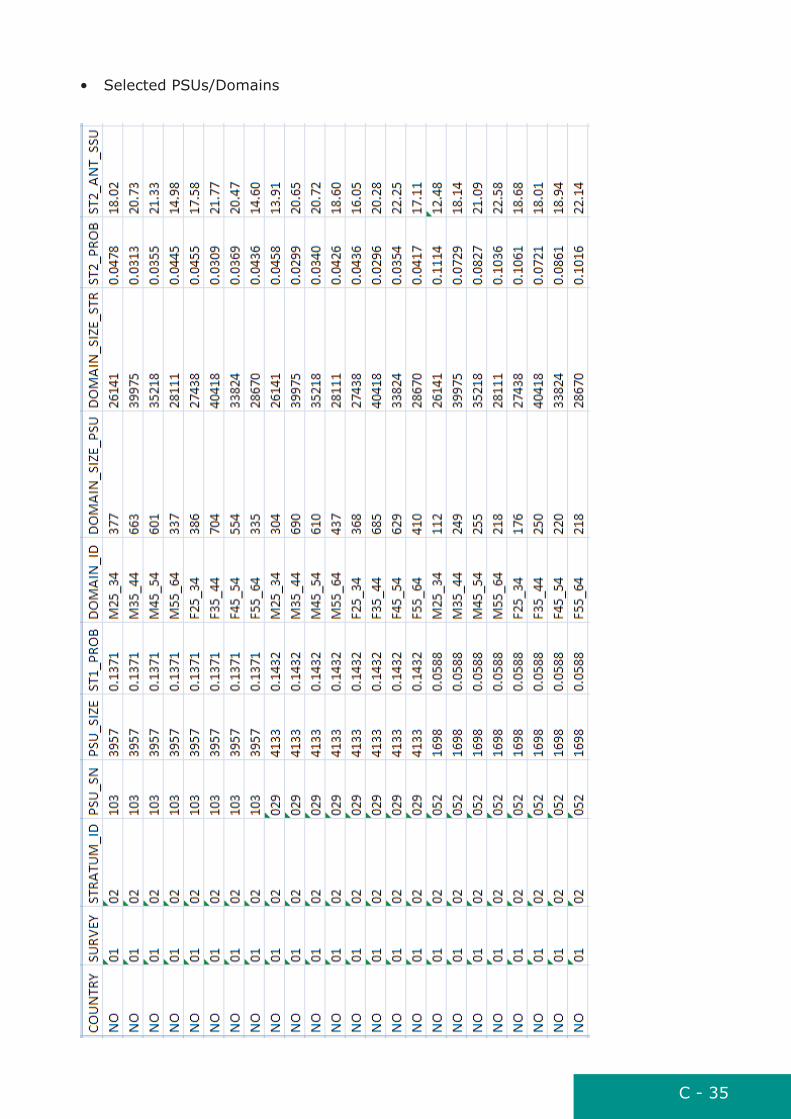
Selected PSUs/Domains (file B)

Data in the format specified here should be submitted for each selected PSU/Domain.







max 3 Stratum identifier code. Key item that uniquely identifies the stratum in the survey. Maximum three digits/characters code. Missing data are not accepted.

PSU_SN integer PSU serial number. Key item that uniquely identifies the PSU in the stratum. Replaces the real PSU ID (e.g. postcode, municipality code etc.) that is used nationally to identify the PSU for data collection. It is recommended that PSU serial numbers run across strata since this will distinguish PSUs even without using the stratum identifier code. A link between the PSU serial number and the real PSU ID should be maintained by the national survey organizer only. Missing data are not accepted.

PSU_SIZE integer The number of SSUs in the sampling frame from which the Stage 2 sample in the PSU will be selected (Ni). notE: This number may deviate from the size measure used to calculate ST1_PROB. Missing data are not accepted.

C - 30


ST1_PROB decimal The stage 1 inclusion probability (πi) used in sampling. Missing data are not accepted.

DOMAIN_ID character string

max 10 relevant if DoMainS > 1. irrelevant = empty field. Domain identifier (for each domain in the PSU). Key item that uniquely identifies the age-sex domain for the record within PSU. Maximum 10 characters. If relevant, missing data are not accepted.

DOMAIN_SIZE_PSU integer relevant if DoMainS > 1. irrelevant = empty field. The number of people in the age-sex domain within PSU (Nid). If relevant, missing data are not accepted.

DOMAIN_SIZE_STR integer relevant if DoMainS > 1. optional if St1_Cv = 2. irrelevant = empty field. The number of people in the age-sex domain in the statum. 99999999 = Missing data.

ST2_PROB decimal The stage 2 inclusion probability (φi) for the PSU or domain. If age-sex stratification is used this probability will be different for different age-sex domains. Missing data are not accepted.

ST2_ANT_SSU decimal Anticipated stage 2 sample size within the PSU or domain (nid). Missing data are not accepted.

Stage 2

Selected persons (file C)

Data in the format specified here should be submitted for each person selected to the sample.




C - 31




SERIAL character string

12 Serial number. Key item that uniquely identifies the person selected to the survey sample. See Part A, Section 12.2 for details. Please make sure always to use the same Serial number for the same person. If the Serial number is less than 12 characters, use leading zeros. Missing data are not accepted.


max 3 Stratum identifier code. Identifies the stratum in the survey. Maximum three digits/characters code. Missing data are not accepted.

PSU_SN integer PSU serial number. Identifies the PSU in the stratum. Replaces the real PSU ID (e.g. postcode, municipality code etc.) that is used nationally to identify the PSU for data collection. It is recommended that PSU serial numbers run across strata since this will distinguish PSUs even without using the stratum identifier code. A link between the PSU serial number and the real PSU ID should be maintained by the national survey organizer only. Missing data are not accepted.

DOMAIN_ID character string

max 10 relevant if DoMainS > 1. irrelevant = empty field. Domain identifier (for each domain in the PSU). Identifies the age-sex domain for the record within PSU. Maximum 10 characters. If relevant, missing data are not accepted.

C - 32


ST2_SEL_SSU integer Number of SSUs actually selected within the PSU or domain. Must be calculated from the sample when the Stage 2 sampling has taken place. All who were selected should be counted here. This concerns also those who were later found to be not eligible to the sample. Missing data are not accepted.

HOUSEHOLD_UNIT integer Are addresses /households used as sampling units? 1 = Yes 2 = No Missing data are not accepted.

HOUSEHOLD_SN character string

max 5 relevant if HouSEHolD_unit = 1. irrelevant = empty field. Address /household code. The code has to be unique in the PSU. Maximum 5 characters. If relevant, missing data are not accepted.

ST3_SAMPLING integer relevant if HouSEHolD_unit = 1. irrelevant = empty field. Was there probability sampling within households? 1= Yes 2 = No If relevant, missing data are not accepted.

ST3_PROB decimal The stage 3 inclusion probability. If ST3_SAMPLING = 1 then ST3_PROB = individual propability. If HOUSEHOLD_UNIT = 2 or ST3_SAMPLING = 2 then ST3_PROB = 1. Missing data are not accepted.

ALL_PROB decimal The overall inclusion probability (πiφi or πiφid) of the person selected to the sample. ALL_PROB = ST1_PROB x ST2_PROB x ST3_PROB. Missing data are not accepted.

C - 33


SAMPLING_WEIGHT decimal The sampling weight (Wi or Wid) of the person selected to the sample. SAMPLING_WEIGHT = 1/ALL_PROB. Missing data are not accepted.

General instructions and examples

The data should be prepared in aSCii format using semicolon (;) as a delimiter between columns (i.e. data items), with the names of the columns in the first row. Each column name should be given either in big letters or in small letters (not both).

To simplify the tracing of data transfers between each country and the EHES Reference Centre, the files should be named as:

EHES_CCXX_YYYYMMDD_n.csv, where

• CC is the country code (e.g. EL for Greece)• XX is the two digit number identifying the survey• YYYYMMDD is the date (year, month and day) when the file

was created (e.g. 20110915)• N is the sequence number of the data transfer file during the

same day (1...n).

C - 34

Examples of data columns:

• Stratification

C - 35

• Selected PSUs/Domains

C - 36

• Selected persons

C - 37

appendix 2b. Data transfer format - Eligibility and participationThe purpose of this transfer format is to provide an exact and common format for EHES countries to transfer the data on eligi-bility to the Reference Centre. Data in the format specified here should be submitted for each person selected to the sample. The selected persons should be defined in section Appendix 2a. Data transfer format - sampling data.


Data items on eligibility are specified in the table below. Within the data transfer file each data item represents one column of data, whereas each row represents a person selected to the sam-ple. The key items for each row are COUNTRY, SURVEY and SE-RIAL. Note that particular data items (e.g. ELIG, EXAM, QUEST) serve as filters to indicate whether another data item is relevant (value is expected) or irrelevant (empty field, leave the value empty).








ELIG integer Eligibility: 1 = Yes 2 = No 3 = Unresolved The definitions for eligiblity, non-eligiblity and unresolved cases are given in Part A, Section 13.2.1. Missing data are not accepted.

C - 38


REASON integer relevant if EliG = 2. Irrelevant = empty field. Reason for non-eligibility: 1 = Died before scheduled examination time 2 = Moved out of the PSU between scheduled time 3 = Erroneus data on sampling frame 4 = Other 5 = Insufficient data If relevant, missing data are not accepted.

EXAM integer relevant if EliG = 1. irrelevant = empty field. Participated in examination: 1 = Yes 2 = No If relevant, missing data are not accepted.

EXAM_REF integer relevant if EliG = 1 and EXaM = 2. irrelevant = empty field. Refused to participate to the examination: 1 = Yes 2 = No 3 = Insufficient data If relevant, missing data are not accepted.

EXAM_NOAPP integer relevant if EliG = 1, EXaM = 2 and EXaM_rEF ≠ 1. irrelevant = empty field. Interested but failed to make appointment for examination. 1 = Yes 2 = No 3 = Insufficient data If relevant, missing data are not accepted.

QUEST integer relevant if EliG = 1. irrelevant = empty field. Completed questionnaire. (At least something filled in to the questionnaire. Code ’no’ only when questionnaire is not returned or is returned completely empty.) 1 = Yes 2 = No If relevant, missing data are not accepted.

C - 39


QUEST_REF integer relevant if EliG = 1 and QuESt = 2. irrelevant = empty field. Refused to participate to questionnaire: 1 = Yes 2 = No 3 = Insufficient data If relevant, missing data are not accepted.

SEX integer Sex: 1 = Male 2 = Female 9 = Missing data Code for missing data is allowed only if - ELIG ≠ 1 or - EliG = 1, EXaM = 2 and QuESt = 2 and the information is not available from the sampling frame or other sources.

AGE integer Age in full years. Derive AGE primarily from the date of birth and the date of examination. If examinations for core measurements were carried out on several days, use the date when most of the examinations were carried out. If this is not available, use age from the questionnaire. 999 = Missing data Code for missing data is allowed only if - ELIG ≠ 1 or - EliG = 1, EXaM = 2 and QuESt = 2 and the information is not available from the sampling frame or other sources.

Consent information for participants to the examination:

CONSENT_ANTR integer relevant if EliG = 1 and EXaM=1. irrelevant = empty field. a. Is there a consent for anthropometric measurements? 1 = Yes 2 = No If relevant, missing data are not accepted.

C - 40


CONSENT_BP integer relevant if EliG = 1 and EXaM=1. irrelevant = empty field. b. Is there a consent for blood pressure measurement? 1 = Yes 2 = No If relevant, missing data are not accepted.

CONSENT_BS integer relevant if EliG = 1 and EXaM=1. irrelevant = empty field. c. Is there a consent for taking blood samples? 1 = Yes 2 = No If relevant, missing data are not accepted.

CONSENT_LIPID integer relevant if EliG = 1, EXaM=1 and ConSEnt_bS = 1. irrelevant = empty field. d. Is there a consent for the measurement of lipids from the blood samples? 1 = Yes 2 = No If relevant, missing data are not accepted.

CONSENT_GLUC integer relevant if EliG = 1, EXaM=1 and ConSEnt_bS = 1. irrelevant = empty field. e. Is there a consent for the measurement of glucose from the blood samples? 1 = Yes 2 = No If relevant, missing data are not accepted.

CONSENT_STORE integer relevant if EliG = 1, EXaM=1 and ConSEnt_bS = 1. irrelevant = empty field. f. Is there a consent for long term storage of blood samples for future analysis? 1 = Yes 2 = No If relevant, missing data are not accepted.

C - 41


CONSENT_DNA integer relevant if EliG = 1, EXaM=1 and ConSEnt_bS = 1. irrelevant = empty field. g. Is there a consent for the analysis of DNA? 1 = Yes 2 = No If relevant, missing data are not accepted.

General instructions


To simplify the tracing of data transfers between each country and the EHES Reference Centre, the file should be named as follows:



was created (e.g. 20110915)• N is the sequence number of the data transfer file during

the same day (1...n).

C - 42

Example of data columns:

• Eligibility

C - 43

appendix 2c. Data transfer format - Question-naire dataThe purpose of this transfer format is to provide an exact and common format for EHES countries to transfer the questionnaire data to the Reference Centre. Data in the format specified here should be submitted for each eligible per-son who completed the questionnaire, as defined in section Appendix 2b. Data transfer format - Eligibility and participation, i.e. for those with ELIG = 1 and QUEST = 1. The data should not be submitted for those who were non-eligible or whose eligibility status is unresolved.

Please make sure that the key items (COUNTRY, SURVEY and SERIAL) for the person are the same as for the data specified in section Appendix 2b. Data transfer format - Eligibility and participation.


Data items on the EHES questionnaire are specified in the table below. Within the data transfer file each data item represents one column of data, whereas each row represents a person who completed the questionnaire. The key items for each row are COUNTRY, SURVEY and SERIAL. Note that particular data items serve as filters to indicate whether another data item is relevant (value is expected) or irrelevant (empty field, leave the value empty).








European Background Module:

C - 44


PERSONS integer How many persons live in the household (including yourself)? 99 = Missing data

SEX_QUEST integer Sex from the questionnaire: 1 = Male 2 = Female 9 = Missing data

AGE_QUEST Self reported age from the questionnaire. 999 = Missing data

BIRTH_YEAR integer Year of birth. Four digit number. 9999 = Missing data

MARIT_STATUS integer What is your legal marital status? 1 = Single (never married) 2 = Married (including registered partnership) 3 = Widowed and not remarried 4 = Divorced and not remarried (including legally separated and dissolved registered partnership) 9 = Missing data

COUPLE integer Are you living with someone as a couple? 1 = Yes 2 = No 9 = Missing data

EDUCATION integer What is the highest education leaving certificate, diploma or education degree you have obtained? 1 = No formal education (or below ISCED1) 2 = Primary education (ISCED1) 3 = Lower secondary education (ISCED2) 4 = Upper secondary education (ISCED3) 5 = Post-secondary but not-tertiary education (ISCED4) 6 = First stage of tertiary education (ISCED5) 7 = Second stage of tertiary education (ISCED6) 9 = Missing data

SCHOOL_YEARS integer How many years have you spent at school or in full-time study? 99 = Missing data

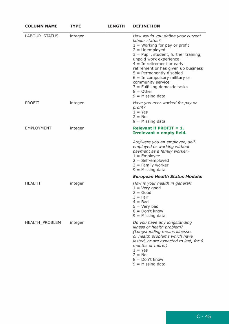
C - 45


LABOUR_STATUS integer How would you define your current labour status? 1 = Working for pay or profit 2 = Unemployed 3 = Pupil, student, further training, unpaid work experience 4 = In retirement or early retirement or has given up business 5 = Permanently disabled 6 = In compulsory military or community service 7 = Fulfilling domestic tasks 8 = Other 9 = Missing data

PROFIT integer Have you ever worked for pay or profit? 1 = Yes 2 = No 9 = Missing data

EMPLOYMENT integer relevant if ProFit = 1. Irrelevant = empty field. Are/were you an employee, self-employed or working without payment as a family worker? 1 = Employee 2 = Self-employed 3 = Family worker 9 = Missing data

European Health Status Module:

HEALTH integer How is your health in general? 1 = Very good 2 = Good 3 = Fair 4 = Bad 5 = Very bad 8 = Don’t know 9 = Missing data

HEALTH_PROBLEM integer Do you have any longstanding illness or health problem? (Longstanding means illnesses or health problems which have lasted, or are expected to last, for 6 months or more.) 1 = Yes 2 = No 8 = Don’t know 9 = Missing data

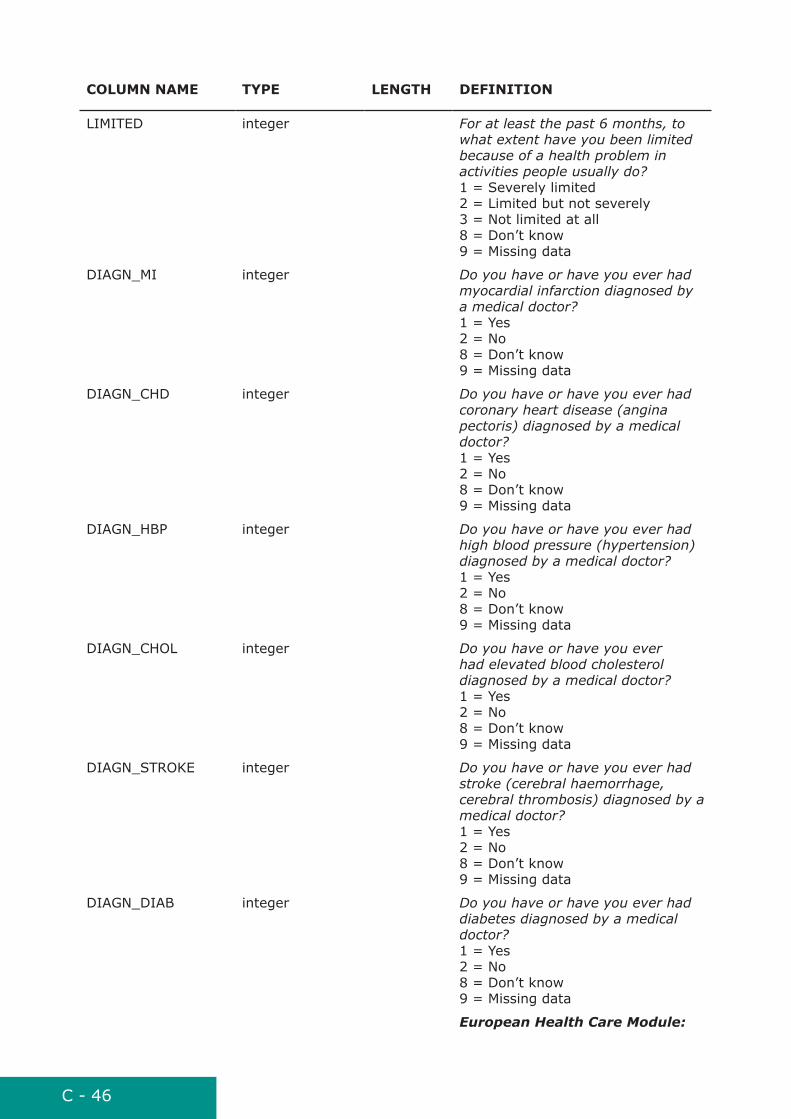
C - 46


LIMITED integer For at least the past 6 months, to what extent have you been limited because of a health problem in activities people usually do? 1 = Severely limited 2 = Limited but not severely 3 = Not limited at all 8 = Don’t know 9 = Missing data

DIAGN_MI integer Do you have or have you ever had myocardial infarction diagnosed by a medical doctor? 1 = Yes 2 = No 8 = Don’t know 9 = Missing data

DIAGN_CHD integer Do you have or have you ever had coronary heart disease (angina pectoris) diagnosed by a medical doctor? 1 = Yes 2 = No 8 = Don’t know 9 = Missing data

DIAGN_HBP integer Do you have or have you ever had high blood pressure (hypertension) diagnosed by a medical doctor? 1 = Yes 2 = No 8 = Don’t know 9 = Missing data

DIAGN_CHOL integer Do you have or have you ever had elevated blood cholesterol diagnosed by a medical doctor? 1 = Yes 2 = No 8 = Don’t know 9 = Missing data

DIAGN_STROKE integer Do you have or have you ever had stroke (cerebral haemorrhage, cerebral thrombosis) diagnosed by a medical doctor? 1 = Yes 2 = No 8 = Don’t know 9 = Missing data

DIAGN_DIAB integer Do you have or have you ever had diabetes diagnosed by a medical doctor? 1 = Yes 2 = No 8 = Don’t know 9 = Missing data

European Health Care Module:

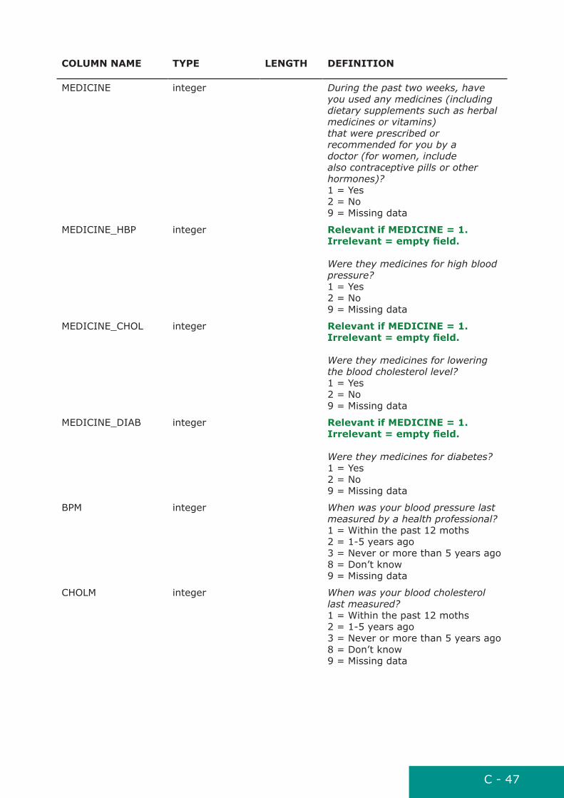
C - 47


MEDICINE integer During the past two weeks, have you used any medicines (including dietary supplements such as herbal medicines or vitamins) that were prescribed or recommended for you by a doctor (for women, include also contraceptive pills or other hormones)? 1 = Yes 2 = No 9 = Missing data

MEDICINE_HBP integer relevant if MEDiCinE = 1. irrelevant = empty field. Were they medicines for high blood pressure? 1 = Yes 2 = No 9 = Missing data

MEDICINE_CHOL integer relevant if MEDiCinE = 1. irrelevant = empty field. Were they medicines for lowering the blood cholesterol level? 1 = Yes 2 = No 9 = Missing data

MEDICINE_DIAB integer relevant if MEDiCinE = 1. irrelevant = empty field. Were they medicines for diabetes? 1 = Yes 2 = No 9 = Missing data

BPM integer When was your blood pressure last measured by a health professional? 1 = Within the past 12 moths 2 = 1-5 years ago 3 = Never or more than 5 years ago 8 = Don’t know 9 = Missing data

CHOLM integer When was your blood cholesterol last measured? 1 = Within the past 12 moths 2 = 1-5 years ago 3 = Never or more than 5 years ago 8 = Don’t know 9 = Missing data

C - 48


GLCM integer When was your blood sugar (glucose) last measured? 1 = Within the past 12 moths 2 = 1-5 years ago 3 = Never or more than 5 years ago 8 = Don’t know 9 = Missing data

European Health Determinants Module:

SHEIGHT integer/decimal How tall are you without shoes (cm)? 8 = Don’t know 9 = Missing data

SWEIGHT integer/decimal How much do you weight without clothes and shoes (kg)? 8 = Don’t know 9 = Missing data

SMOKE integer Do you smoke at all nowadays? 1 = Yes, daily 2 = Yes, occasionally 3 = Not at all 9 = Missing data

What tobacco product do you smoke each day:

SMOKE_CIGSM integer relevant if SMoKE = 1. irrelevant = empty field. a. Manufactured cigarettes? 1 = Yes 2 = No 9 = Missing data

SMOKE_CIGSH integer relevant if SMoKE = 1. irrelevant = empty field. b. Hand-rolled cigarettes? 1 = Yes 2 = No 9 = Missing data

SMOKE_CIGARS integer relevant if SMoKE = 1. irrelevant = empty field. c. Cigars? 1 = Yes 2 = No 9 = Missing data

SMOKE_PIPE integer relevant if SMoKE = 1. irrelevant = empty field. d. Pipefuls of tobacco? 1 = Yes 2 = No 9 = Missing data

C - 49


SMOKE_OTHER integer relevant if SMoKE = 1. irrelevant = empty field. e. Other? 1 = Yes 2 = No 9 = Missing data

On average, how many cigarettes, cigars or pipefuls do you smoke each day:

NUM_CIGSM integer relevant if SMoKE_CiGSM = 1. irrelevant = empty field. a. Manufactured cigarettes? 999 = Missing data

NUM_CIGSH integer relevant if SMoKE_CiGSH = 1. irrelevant = empty field. b. Hand-rolled cigarettes? 999 = Missing data

NUM_CIGARS integer relevant if SMoKE_CiGarS = 1. irrelevant = empty field. c. Cigars? 999 = Missing data

NUM_PIPE integer relevant if SMoKE_PiPE = 1. irrelevant = empty field. d. Pipefuls of tobacco? 999 = Missing data

NUM_OTHER integer relevant if SMoKE_otHEr = 1. irrelevant = empty field. e. Other? 999 = Missing data

SMOKE_EVER integer Relevant if SMOKE ≠ 1. irrelevant = empty field. Have you ever smoked (cigarettes, cigars, pipes) daily, or almost daily, for at least one year? 1 = Yes 2 = No 9 = Missing data

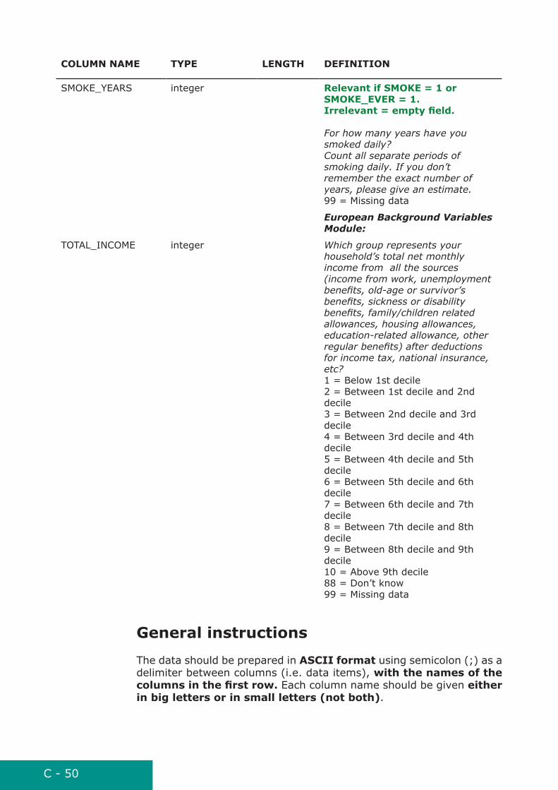
C - 50


SMOKE_YEARS integer relevant if SMoKE = 1 or SMoKE_EvEr = 1. irrelevant = empty field. For how many years have you smoked daily? Count all separate periods of smoking daily. If you don’t remember the exact number of years, please give an estimate. 99 = Missing data

European Background Variables Module:

TOTAL_INCOME integer Which group represents your household’s total net monthly income from all the sources (income from work, unemployment benefits, old-age or survivor’s benefits, sickness or disability benefits, family/children related allowances, housing allowances, education-related allowance, other regular benefits) after deductions for income tax, national insurance, etc? 1 = Below 1st decile 2 = Between 1st decile and 2nd decile 3 = Between 2nd decile and 3rd decile 4 = Between 3rd decile and 4th decile 5 = Between 4th decile and 5th decile 6 = Between 5th decile and 6th decile 7 = Between 6th decile and 7th decile 8 = Between 7th decile and 8th decile 9 = Between 8th decile and 9th decile 10 = Above 9th decile 88 = Don’t know 99 = Missing data



C - 51



• CC is the country code (e.g. EL for Greece)• XX is the two digit number identifying the survey• YYYYMMDD is the date (year, month and day) when the

file was created (e.g. 20110915)• N is the sequence number of the data transfer file during

the same day (1...n).

C - 52

appendix 2d. Data transfer format - Measurements dataThe purpose of this transfer format is to provide an exact and common format for EHES countries to transfer the data on the core measurements to the Reference Centre. Data in the format specified here should be submitted for each eligible person who participated in examination, as defined in section Appendix 2b. Data transfer format - Eligibility and participation, i.e. for those with ELIG = 1 and EXAM = 1. The data should not be submitted for those who were non-eligible or whose eligibility status is un-resolved.

Please make sure that the key items (COUNTRY, SURVEY and SERIAL) for the person are the same as for the data specified in section Appendix 2b. Data transfer format - Eligibility and par-ticipation.


Data items on the core measurements are specified in the table below. Within the data transfer file each data item represents one column of data, whereas each row represents a person who par-ticipated in examination. The key items for each row are COUN-TRY, SURVEY and SERIAL. Note that particular data items serve as filters to indicate whether another data item is relevant (value is expected) or irrelevant (empty field, leave the value empty).






C - 53




Blood pressure:

BP_MISSING integer Reason if not measured at all. relevant if all measurement values (bP_SYSt and bP_DiaSt) are coded as 999. Irrelevant = empty field. Medical reason preventing blood pressure measurement: 1 = Amputation of both arms 2 = Cast on both arms 3 = Open wounds/sores on both arms 4 = Rash on both arms 5 = Malformation of both arms preventing to place the cuff 6 = Lymph node malfunction in both arms e.g. caused by breast cancer and preventing to place the cuff 10 = Other medical reason 11 = Refusal (includes those who did not give consent for blood pressure measurement: see item CONSENT_BP in section Eligibility an participation (Appendix 2b). If CONSENT_BP = 2 then BP_MISSING = 11.) 88 = Other 99 = Missing data

BP_CODER character string (max) 12 Measurer’s identification code. Maximum 12 characters. NNNNN = Missing data

BP_DATE character string 8 Date of the measurement. Date format YYYYMMDD: year (4 digits), month (2 digits), day (2 digits). Express month and day with a leading zero if needed. If blood pressure was not measured, code the date when the person attended the examinations. If the exact day is not known, code DD=99.

C - 54


BP_TIME character string 5 Time (hour:minute) of the measurement. Express hour and minute with two digits, use a leading zero if needed. If the minutes are not known, code minute=99. 99:99 = Missing data

BP_ROOMTEMP integer/decimal Room temperature during blood pressure measurement (oC). 99 = Missing data

BP_EXERCISED integer Has participant done vigorous physical exercise one hour before blood pressure measurement? 1 = Yes 2 = No 9 = Missing data

BP_SMOKED integer Has participant smoked one hour before blood pressure measurement? 1 = Yes 2 = No 9 = Missing data

BP_EATEN integer Has participant eaten one hour before blood pressure measurement? 1 = Yes 2 = No 9 = Missing data

BP_DRANK integer Has participant drank anything else than water one hour before blood pressure measurement? 1 = Yes 2 = No 9 = Missing data

BP_BLADDER integer Has participant emtied his/her bladder one hour before blood pressure measurement? 1 = Yes 2 = No 9 = Missing data

BP_DEVICE integer Type of the measurement device: 1 = Mercury sphygmomanometer 2 = Automated device 8 = Other 9 = Missing data

BP_DEVICENO integer Number of the measurement device. 999 = Missing data

BP_ARM integer Arm used for the measurement: 1 = Right 2 = Left 9 = Missing data

C - 55


BP_ARMLEFT integer relevant if bP_arM = 2. irrelevant = empty field. Reason for use of left arm. Medical reason: 1 = Paralized and/or spastic right arm 2 = Amputation of right arm 3 = Cast on right arm 4 = Open wounds/sores on right arm 5 = Rash on right arm 6 = Intravenous access device on right arm 7 = Malformation of right arm preventing to place the cuff 8 = Lymph node malfunction in right arm e.g. caused by beast cancer and preventing to place the cuff 88 = Other 99 = Missing data

BP_ARMC decimal (0.5) Arm circumference in cm. Round to 0.5 cm. 99.9 = Missing data

BP_CUFF integer Used cuff size: 1 = Small 2 = Medium 3 = Large 4 = Extra large 9 = Missing data

BP_POSTURE integer Posture of the subject during the measurement: 1 = Sitting 2 = Supine 9 = Missing data

BP_POSTURE_EX integer relevant if bP_PoSturE = 2. irrelevant = empty field. Reason for supine posture: 1 = Bed driven 8 = Other 9 = Missing data

BP_PULSE integer Pulse rate (60 seconds). 999 = Missing data

BP_PULSEREG integer Was the pulse regular? 1 = Yes 2 = No 9 = Missing data

BP_SYST1 integer Systolic blood pressure (mmHg): 1st measurement. 999 = missing data

C - 56


BP_DIAST1 integer Diastolic blood pressure (mmHg): 1st measurement. 999 = missing data

BP_SYST2 integer Systolic blood pressure (mmHg): 2nd measurement. 999 = missing data

BP_DIAST2 integer Diastolic blood pressure (mmHg): 2nd measurement. 999 = missing data

BP_SYST3 integer Systolic blood pressure (mmHg): 3rd measurement. 999 = missing data

BP_DIAST3 integer Diastolic blood pressure (mmHg): 3rd measurement. 999 = missing data

Height:

HEIGHT_MISSING integer Reason if not measured at all. relevant if HEiGHt = 999.9 . irrelevant = empty field. Reason codes: 1 = Hairstyle or headdress prevents measurement (not possible to undress) 2 = Wheelchair bound or immobile 3 = Unsteady stand 4 = Height exceeds the upper limit of the stadiometer. Specify the upper limit of the stadiometer. 5 = Refusal (includes those who did not give consent for anthropometric measurements: see item CONSENT_ANTR in section Eligibility and particaption (Appendix 2b). If CONSENT_ANTR = 2 then HEIGHT_MISSING = 5.) 8 = Other 9 = Missing data

HEIGHT_ULIMIT decimal (0.1) relevant if HEiGHt_MiSSinG = 4. irrelevant = empty field. Specify the upper limit of the stadiometer in cm. Round to 0.1 cm. 999.9 = Missing data

HEIGHT_CODER character string (max) 12 Measurer’s identification code. Maximum 12 characters. NNNNN = Missing data

HEIGHT_DEVICENO integer Number of the measurement device. 999 = Missing data

C - 57


HEIGHT decimal (0.1) Height in cm. Round to 0.1 cm. 999.9 = Missing data

Weight:

WEIGHT_MISSING integer Reason if not measured at all. relevant if WEiGHt = 999.99 . irrelevant = empty field. Reason codes: 1 = Wheelchair bound or immobile 2 = Unsteady stand 3 = Weight exceeds the upper limit of the scale. Specify the upper limit of the scale. 4 = Refusal (includes those who did not give consent for anthropometric measurements: see item CONSENT_ANTR in section Eligibility and participation (Appendix 2b). If CONSENT_ANTR = 2 then WEIGHT_MISSING = 4.) 8 = Other 9 = Missing data

PREGN integer Is participant pregnant? 1 = Yes 2 = No 9 = Missing data

PREGNWK integer relevant if PrEGn = 1. irrelevant = empty field. Pregnancy week. 99 = Missing data

WEIGHT_ULIMIT decimal (0.01) relevant if WEiGHt_MiSSinG = 3. irrelevant = empty field. Specify the upper limit of the scale in kg. Round to 0.01 kg. 999.99 = Missing data

WEIGHT_CODER character string (max) 12 Measurer’s identification code. Maximum 12 characters. NNNNN = Missing data

WEIGHT_DEVICENO integer Number of the measurement device. 999 = Missing data

WEIGHT_CLOTH integer Measurement was done in: 1 = Light underwear 2 = Without heavy outer garments 8 = Other 9 = Missing data

C - 58


WEIGHT decimal (0.01) Weight in kg. Round to 0.01 kg. 999.99 = Missing data

Waist circumference:

WAIST_MISSING integer Reason if not measured at all. relevant if WaiSt = 999.9 . irrelevant = empty field. Reason codes: 1 = Wheelchair bound of immobile or cannot stand 2 = Unsteady stand 3 = Circumference exceeds the upper limit of the tape. Specify the length of the tape. 4 = Large hernia, stomage bag or other device on measurement area 5 = Refusal (includes those who did not give consent for anthropometric measurements: see item CONSENT_ANTR in section Eligibility and participation (Appendix 2b). If CONSENT_ANTR = 2 then WAIST_MISSING = 5.) 8 = Other 9 = Missing data

WAIST_ULIMIT decimal (0.5) relevant if WaiSt_MiSSinG = 3. irrelevant = empty field. Specify the length of the tape in cm. Round to 0.5 cm. 999.9 = Missing data

WAIST_CODER character string (max) 12 Measurer’s identification code. Maximum 12 characters. NNNNN = Missing data

WAIST_DEVICENO integer Number of the measurement tape. 999 = Missing data

WAIST_CLOTH integer Measurement was done over: 1 = Bare skin 2 = Light underwear 3 = Without thick outer garments 8 = Other 9 = Missing data

WAIST decimal (0.5) Waist circumference in cm. Round to 0.5 cm. 999.9 = Missing data

C - 59






was created (e.g. 20110915)

C - 60

appendix 2e. Data transfer format - laboratory dataThe purpose of this transfer format is to provide an exact and common format for EHES countries to transfer the data on the laboratory sam-ples to the Reference Centre. Data in the format specified here should be submitted for each eligible person who participated in examination, as defined in section Appendix 2b. Data transfer format - Eligibility and participation, i.e. for those with ELIG = 1 and EXAM = 1. The data should not be submitted for those who were non-eligible or whose eli-gibility status is unresolved.

Please make sure that the key items (COUNTRY, SURVEY and SERIAL) for the person are the same as for the data specified in section Appen-dix 2b. Data transfer format - Eligibility and participation.


Data items on the laboratory samples are specified in the table below. Within the data transfer file each data item represents one column of data, whereas each row represents a person who participated in exam-ination. The key items for each row are COUNTRY, SURVEY and SERI-AL. Note that particular data items serve as filters to indicate whether another data item is relevant (value is expected) or irrelevant (empty field, leave the value empty).








C - 61


BS_MISSING integer Reason for missing blood samples. relevant if all measurement values (bS_CHol, bS_HDl, bS_GlC, bS_Hba1C) are coded as 9999.99. Irrelevant = empty field. Reason codes: 1 = Vein could not be found/ difficult to take a blood sample 2 = Refusal (includes those who did not give consent for blood samples: see item CONSENT_BS in section Eligibility and participation (Appendix 2b). If CONSENT_BS = 2 in the eligibility data, BS_MISSING = 2.) 8 = Other 9 = Missing data

BS_CODER character string (max) 12 Identification code of person drawing the blood samples. Maximum 12 characters. NNNNN = Missing data

BS_DATE character string 8 Date of the sample collection. Date format YYYYMMDD: year (4 digits), month (2 digits), day (2 digits). Express month and day with a leading zero if needed. If the exact day is not known, code DD=99. 99999999 = Missing data

BS_TIME character string 5 Time (hour:minute) of the sample collection. Express hour and minute with two digits, use a leading zero if needed. If the minutes are not known, code minute=99. 99:99 = Missing data

BS_ROOMTEMP integer/decimal Room temperature during the sample collection (oC). 99 = Missing data

BS_FAST integer Has participant fasted at least 8 hours? 1 = Yes 2 = No 9 = Missing data

BS_TIME_MEAL character string 5 Time (hour:minute) of the last meal or sweetened drink. Express hour and minute with two digits, use a leading zero if needed. If the minutes are not known, code minute=99. 99:99 = Missing data

C - 62


BS_POSTURE integer Posture of the subject during the blood collection: 1 = Sitting 2 = Supine 9 = Missing data

BS_POSTURE_EX integer relevant if bS_PoSturE = 2. irrelevant = empty field. Reason for supine posture: 1 = Fainting 2 = Bed driven 8 = Other 9 = Missing data

BS_ARM integer Arm used for blood collection (if blood collection failed, code the arm where the last attempt was made): 1 = Left 2 = Right 9 = Missing data

BS_ARMRIGHT integer relevant if bS_arM = 2. irrelevant = empty field. Reason for use of right arm. Medical reason: 1 = No vein found on left arm 2 = No left arm/ Amputation of left arm 3 = Cast on left arm 8 = Other 9 = Missing data

BS_TUBES integer Number of collected tubes. 99 = Missing data

BS_HEMOLYSED integer Number of hemolysed sample tubes. 99 = Missing data

BS_DATE_CTRF character string 8 Date of centrifuging the samples. Date format YYYYMMDD: year (4 digits), month (2 digits), day (2 digits). Express month and day with a leading zero if needed. If the exact day is not known, code DD=99. 99999999 = Missing data

BS_TIME_CTRF character string 5 Time (hour:minute) of centrifuging the samples. Express hour and minute with two digits, use a leading zero if needed. If the minutes are not known, code minute=99. 99:99 = Missing data

C - 63


BS_DATE_FR20 character string 8 Date of freezing the samples to at least -20 °C. Date format YYYYMMDD: year (4 digits), month (2 digits), day (2 digits). Express month and day with a leading zero if needed. If the exact day is not known, code DD=99. 99999999 = Missing data

BS_TIME_FR20 character string 5 Time (hour:minute) of freezing the samples to at least -20 °C. Express hour and minute with two digits, use a leading zero if needed. If the minutes are not known, code minute=99. 99:99 = Missing data

BS_DATE_FR70 character string 8 Date of transferring samples to at least -70 °C. Date format YYYYMMDD: year (4 digits), month (2 digits), day (2 digits). Express month and day with a leading zero if needed. If the exact day is not known, code DD=99. 99999999 = Missing data

BS_DATE_LIPID character string 8 Date of lipid analysis. Date format YYYYMMDD: year (4 digits), month (2 digits), day (2 digits). Express month and day with a leading zero if needed. If the exact day is not known, code DD=99. 99999999 = Missing data

BS_DATE_GLC character string 8 Date of glucose analysis. Date format YYYYMMDD: year (4 digits), month (2 digits), day (2 digits). Express month and day with a leading zero if needed. If the exact day is not known, code DD=99. 99999999 = Missing data

BS_CHOL decimal/integer Serum total cholesterol. Use the unit (mmol/L or mg/dL) in which the value was obtained from the laboratory. If both units are available, mmol/L is preferred. The unit is given in item BS_UNIT_CHOL. 9999.99 = Missing data

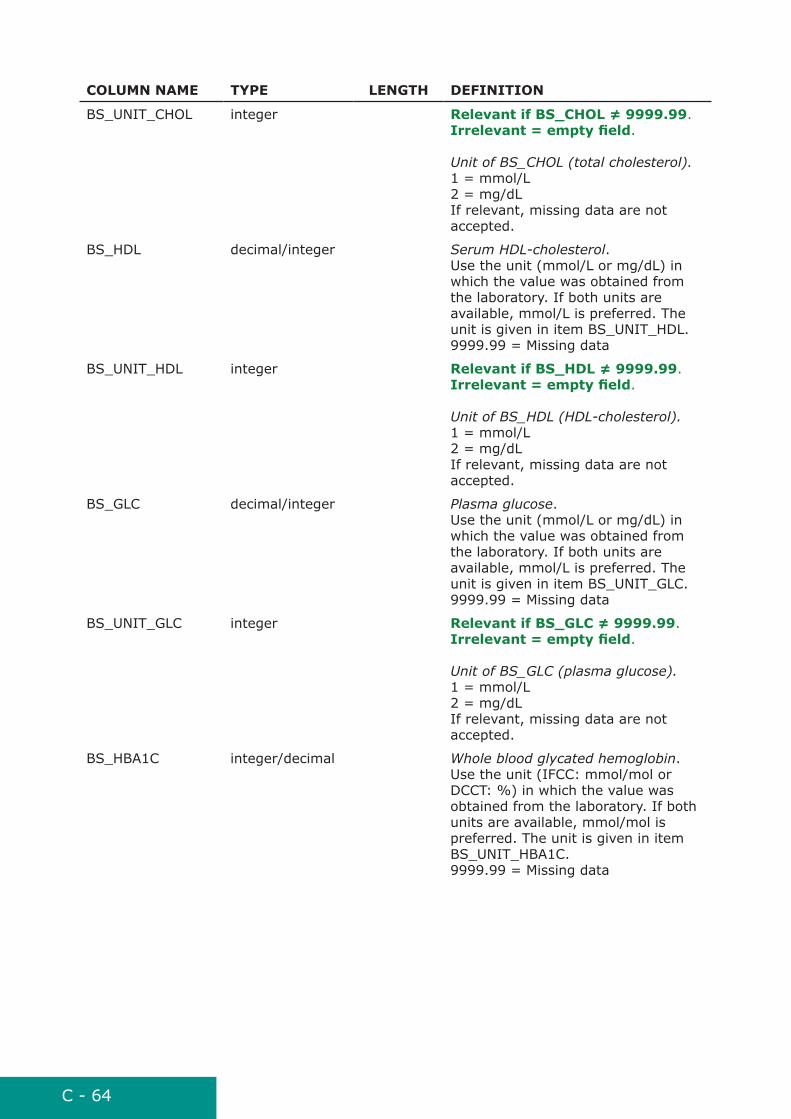
C - 64


BS_UNIT_CHOL integer Relevant if BS_CHOL ≠ 9999.99. irrelevant = empty field. Unit of BS_CHOL (total cholesterol). 1 = mmol/L 2 = mg/dL If relevant, missing data are not accepted.

BS_HDL decimal/integer Serum HDL-cholesterol. Use the unit (mmol/L or mg/dL) in which the value was obtained from the laboratory. If both units are available, mmol/L is preferred. The unit is given in item BS_UNIT_HDL. 9999.99 = Missing data

BS_UNIT_HDL integer Relevant if BS_HDL ≠ 9999.99. irrelevant = empty field. Unit of BS_HDL (HDL-cholesterol). 1 = mmol/L 2 = mg/dL If relevant, missing data are not accepted.

BS_GLC decimal/integer Plasma glucose. Use the unit (mmol/L or mg/dL) in which the value was obtained from the laboratory. If both units are available, mmol/L is preferred. The unit is given in item BS_UNIT_GLC. 9999.99 = Missing data

BS_UNIT_GLC integer Relevant if BS_GLC ≠ 9999.99. irrelevant = empty field. Unit of BS_GLC (plasma glucose). 1 = mmol/L 2 = mg/dL If relevant, missing data are not accepted.

BS_HBA1C integer/decimal Whole blood glycated hemoglobin. Use the unit (IFCC: mmol/mol or DCCT: %) in which the value was obtained from the laboratory. If both units are available, mmol/mol is preferred. The unit is given in item BS_UNIT_HBA1C. 9999.99 = Missing data

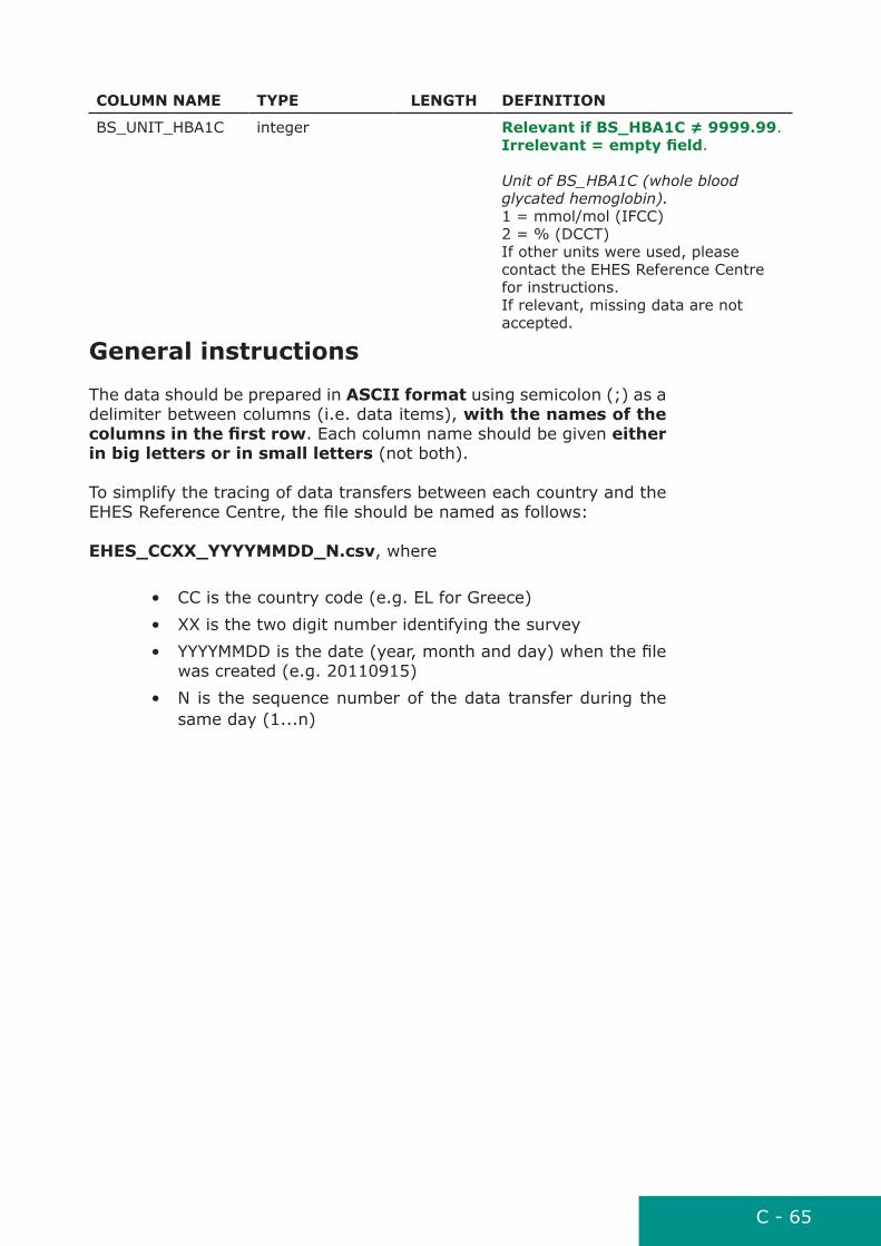
C - 65


BS_UNIT_HBA1C integer Relevant if BS_HBA1C ≠ 9999.99. irrelevant = empty field. Unit of BS_HBA1C (whole blood glycated hemoglobin). 1 = mmol/mol (IFCC) 2 = % (DCCT) If other units were used, please contact the EHES Reference Centre for instructions. If relevant, missing data are not accepted.






was created (e.g. 20110915)• N is the sequence number of the data transfer during the

same day (1...n)

C - 66

appendix 2f. FaQ of the data transferQ1. Do we need separate datasets for each section i.e. sampling, eligi-bility, EHES questionnaire, and measurement data?

• anSWEr: Yes, this is the clearest way. Especially for the sampling data three separate but related data trans-fer files are needed (one for stratification, one for the selected PSUs/Domains, and one for the selected per-sons). It is important is that the key items (with the exception of the first two sampling files these are COUNTRY, SURVEY and SERIAL) are always included. The data transfer files should be named as EHES_CCXX_YYYYMMDD_N.csv, where

• CC is the country code (e.g. EL for Greece)• XX is the two digit number identifying the survey• YYYYMMDD is the date (year, month and day) when

the file was created (e.g. 20110915)• N is the sequence number of the data transfer file

during the same day (1...n).

Q2. Who is considered an eligible participant?

• anSWEr: The concept of eligibility is defined in Part A, Section 13.2.1. (E.g. persons who died or moved out of the primarily sampling unit prior to the scheduled examination are not eligible.) The reason for non-eligibility should be coded with item REASON.

Q3. In datasets for sampling and eligibility all sampled population need to be included. How is it with the other datasets which include the ac-tual survey data? Do we still include the whole sample and just leave the data blank for the questionnaire and examination portions?

• anSWEr: No, you will need to include all sampled popu-lation only in datasets for sampling and eligibility. For the other datasets (actual survey data) you need to include only those subjects who are eligible and who participated in ex-amination and/or completed the questionnaire. However, it is important that the data on each person’s eligiblity status matches the data on examination and questionnaire files. (E.g. if ELIG = 1 and EXAM = 1 in the eligibility data, there should exist a row for the same SERIAL number in the ex-amination data.)

C - 67

Q4. Regarding the questionnaire dataset some of our questions devi-ate from the final version of the EHES core questionnaire. Should we code these questions in the dataset as we have coded them and go into detail on deviations in the supporting documents?

• anSWEr: The questions should be coded according to the questionnaire definition (Appendix 2c) given here. For the data items which are not one-on-one you need to prepare a document describing how you have derived these data items from your local data. If you have any detailed ques-tions about this, please contact the EHES Reference Centre.

Q5. In cases where we did not include certain questions (for example did not ask about last blood pressure measurement or include genetic testing), should we include data on the question in our datasets and simply code them as missing or should we exclude it all together?

• anSWEr: You need to include data on these kind of ques-tions in the datasets and code them as missing data.

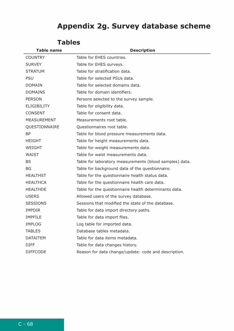
C - 68

appendix 2g. Survey database scheme

tablestable name Description

COUNTRY Table for EHES countries.

SURVEY Table for EHES surveys.

STRATUM Table for stratification data.

PSU Table for selected PSUs data.

DOMAIN Table for selected domains data.

DOMAINS Table for domain identifiers.

PERSON Persons selected to the survey sample.

ELIGIBILITY Table for eligibility data.

CONSENT Table for consent data.

MEASUREMENT Measurements root table.

QUESTIONNAIRE Questionnaires root table.

BP Table for blood pressure measurements data.

HEIGHT Table for height measurements data.

WEIGHT Table for weight measurements data.

WAIST Table for waist measurements data.

BS Table for laboratory measurements (blood samples) data.

BG Table for background data of the questionnaire.

HEALTHST Table for the questionnaire health status data.

HEALTHCA Table for the questionnaire health care data.

HEALTHDE Table for the questionnaire health determinants data.

USERS Allowed users of the survey database.

SESSIONS Sessions that modified the state of the database.

IMPDIR Table for data import directory paths.

IMPFILE Table for data import files.

IMPLOG Log table for imported data.

TABLES Database tables metadata.

DATAITEM Table for data items metadata.

DIFF Table for data changes history.

DIFFCODE Reason for data change/update: code and description.

C - 69

Graph of the survey database in pdf

QUESTIONNAIRE

ID NUMBER(38)

PID NUMBER(38)

STATUS NUMBER(1)

BG

QID NUMBER(38)

PERSONS NUMBER(2)

SEX NUMBER(1)

AGE NUMBER(3)

BIRTH_YEAR NUMBER(4)

MARIT_STATUS NUMBER(1)

COUPLE NUMBER(1)

EDUCATION NUMBER(1)

SCHOOL_YEARS NUMBER(2)

LABOUR_STATUS NUMBER(1)

PROFIT NUMBER(1)

EMPLOYMENT NUMBER(1)

TOTAL_INCOME NUMBER(2)

MEASUREMENT

ID NUMBER(38)

PID NUMBER(38)

STATUS NUMBER(1)

BP

MID NUMBER(38)

MISSING NUMBER(2)

CODER VARCHAR2(12)

DATE CHAR(8)

TIME CHAR(5)

ROOMTEMP NUMBER

EXERCISED NUMBER(1)

SMOKED NUMBER(1)

EATEN NUMBER(1)

DRANK NUMBER(1)

BLADDER NUMBER(1)

DEVICE NUMBER(1)

DEVICENO NUMBER(15)

ARM NUMBER(1)

ARMLEFT NUMBER(2)

ARMC NUMBER

CUFF NUMBER(1)

POSTURE NUMBER(1)

POSTURE_EX NUMBER(1)

PULSE NUMBER(3)

PULSEREG NUMBER(1)

SYST1 NUMBER(3)

DIAST1 NUMBER(3)

SYST2 NUMBER(3)

DIAST2 NUMBER(3)

SYST3 NUMBER(3)

DIAST3 NUMBER(3)

BS

MID NUMBER(38)

MISSING NUMBER(1)

CODER VARCHAR2(12)

DATE CHAR(8)

TIME CHAR(5)

ROOMTEMP NUMBER(2)

FAST NUMBER(1)

TIME_MEAL CHAR(5)

POSTURE NUMBER(1)

POSTURE_EX NUMBER(1)

ARM NUMBER(1)

ARMRIGHT NUMBER(1)

TUBES NUMBER(2)

HEMOLYSED NUMBER(2)

DATE_CTRF CHAR(8)

TIME_CTRF CHAR(5)

DATE_FR20 CHAR(8)

TIME_FR20 CHAR(5)

DATE_FR70 CHAR(8)

DATE_LIPID CHAR(8)

DATE_GLC CHAR(8)

CHOL NUMBER

UNIT_CHOL NUMBER(1)

HDL NUMBER

UNIT_HDL NUMBER(1)

GLC NUMBER

UNIT_GLC NUMBER(1)

HBA1C NUMBER

UNIT_HBA1C NUMBER(1)

PERSON

ID NUMBER(38)

COUNTRY_ID NUMBER(38)

SURVEY_ID NUMBER(38)

SERIAL CHAR(12)

DOMAIN_ID NUMBER(38)

HOUSEHOLD_UNIT NUMBER(1)

HOUSEHOLD_SN CHAR(5)

ST3_SAMPLING NUMBER(1)

ST3_PROB NUMBER

ALL_PROB NUMBER

SAMPLING_WEIGHT NUMBER

SEX NUMBER(1)

AGE NUMBER(3)

STATUS NUMBER(1)

CONSENT

PID NUMBER(38)

ANTR NUMBER(1)

BP NUMBER(1)

BS NUMBER(1)

LIPID NUMBER(1)

GLC NUMBER(1)

STORE NUMBER(1)

DNA NUMBER(1)

COUNTRY

ID NUMBER(38)

NAME VARCHAR2(15)

CODE CHAR(2)

JA NUMBER(1)

TABLES

ID NUMBER(38)

NAME VARCHAR2(50)

DATATYPE NUMBER(1)

ORDERNO NUMBER(1)

DESCRIPTION VARCHAR2(500)

DATAITEM

ID NUMBER(38)

ITEM VARCHAR2(30)

TABLES_ID NUMBER(38)

COL VARCHAR2(30)


STATUS NUMBER(1)

CREATED DATE

UPDATED DATE

DIFF

ID NUMBER(38)

IMPLOG_ID NUMBER(38)

DATAITEM_ID NUMBER(38)

ROW_ID NUMBER(38)

VAL_OLD CHAR(8)

VAL_NEW CHAR(8)

CODE NUMBER(38)

DIFFCODE

CODE NUMBER(38)


IMPLOG

ID NUMBER(38)

IMPFILE_ID NUMBER(38)


TABLES_ID NUMBER(38)

DOMAINS

ID NUMBER(38)

DOMAIN_ID VARCHAR2(10)

DOMAIN

ID NUMBER(38)

PSU_ID NUMBER(38)

DOMAINS_ID NUMBER(38)

SIZE_PSU NUMBER(38)

SIZE_STR NUMBER(38)

ST2_PROB NUMBER

ST2_ANT_SSU NUMBER

ST2_SEL_SSU NUMBER(38)

STATUS NUMBER(1)

PSU

ID NUMBER(38)

STRATUM_ID NUMBER(38)

SN NUMBER(38)

SIZE NUMBER(38)

ST1_PROB NUMBER(38,5)

ELIGIBILITY

PID NUMBER(38)

ELIG NUMBER(1)

REASON NUMBER(1)

EXAM NUMBER(1)

EXAM_REF NUMBER(1)

EXAM_NOAPP NUMBER(1)

QUEST NUMBER(1)

QUEST_REF NUMBER(1)

HEALTHCA

QID NUMBER(38)

MED NUMBER(1)

MED_HBP NUMBER(1)

MED_CHOL NUMBER(1)

MED_DIAB NUMBER(1)

BPM NUMBER(1)

CHOLM NUMBER(1)

GLCM NUMBER(1)

HEALTHDE

QID NUMBER(38)

SHEIGHT NUMBER

SWEIGHT NUMBER

SMOKE NUMBER(1)

CIGSM NUMBER(1)

CIGSH NUMBER(1)

CIGARS NUMBER(1)

PIPE NUMBER(1)

OTHER NUMBER(1)

NUM_CIGSM NUMBER(3)

NUM_CIGSH NUMBER(3)

NUM_CIGARS NUMBER(3)

NUM_PIPE NUMBER(3)

NUM_OTHER NUMBER(3)

SMOKE_EVER NUMBER(1)

SMOKE_YEARS NUMBER(2)

HEALTHST

QID NUMBER(38)

HEALTH NUMBER(1)

HEALTH_PROBLEM NUMBER(1)

LIMITED NUMBER(1)

DIAGN_MI NUMBER(1)

DIAGN_CHD NUMBER(1)

DIAGN_HBP NUMBER(1)

DIAGN_CHOL NUMBER(1)

DIAGN_STROKE NUMBER(1)

DIAGN_DIAB NUMBER(1)

HEIGHT

MID NUMBER(38)

MISSING NUMBER(1)

ULIMIT NUMBER

CODER VARCHAR2(12)

DEVICENO NUMBER(15)

HEIGHT NUMBER

IMPDIR

ID NUMBER(38)

PATH VARCHAR2(250)

IMPFILE

ID NUMBER(38)

IMPDIR_ID NUMBER(38)

FILENAME VARCHAR2(250)

DATE_N VARCHAR2(10)

SESSION_ID NUMBER(38)

SESSIONS

ID NUMBER(38)

USER_ID NUMBER(38)

SESSION_DATE DATE

SURVEY

ID NUMBER(38)

COUNTRY_ID NUMBER(38)

NO CHAR(2)

PILOT VARCHAR2(3)

PERIOD VARCHAR2(40)


STATUS NUMBER(1)

CREATED_ID NUMBER(38)

UPDATED_ID NUMBER(38)

STRATUM

ID NUMBER(38)


CODE CHAR(3)

NAME VARCHAR2(30)

SIZE NUMBER(38)

DOMAINS NUMBER(2)

ST1_ANT_SSU NUMBER

ST1_NO_PSU NUMBER(38)

ST1_SEL_PSU NUMBER(38)

ST1_CV NUMBER(1)

ST1_CPSU NUMBER(38)

ST1_CSSU NUMBER(38)

ST1_COST NUMBER(38)

ST1_VWITHIN NUMBER

ST1_VAMONG NUMBER

STATUS NUMBER(1)

USERS

ID NUMBER(38)

USERNAME VARCHAR2(10)

FULLNAME VARCHAR2(50)

STATUS NUMBER(1)

CREATED DATE

UPDATED DATE

WAIST

MID NUMBER(38)

MISSING NUMBER(1)

ULIMIT NUMBER

CODER VARCHAR2(12)

DEVICENO NUMBER(15)

CLOTH NUMBER(1)

WAIST NUMBER

WEIGHT

MID NUMBER(38)

MISSING NUMBER(1)

PREGN NUMBER(1)

PREGNWK NUMBER(2)

ULIMIT NUMBER

CODER VARCHAR2(12)

DEVICENO NUMBER(15)

CLOTH NUMBER(1)

WEIGHT NUMBER

C - 70

views

view Description

V_BG View for the background data of the questionnaire. Used in QA reports.

V_BP View for the blood pressure data. Used in QA reports.

V_BS View for the blood sample data. Used in QA reports.

V_DATAITEM View for the data items and columns metadata.

V_ELIGCONSENT View for the eligibility and consent data.

V_HEALTHCA View for the healthcare data of the questionnaire. Used in QA reports.

V_HEALTHDE View for the health determinants data of the questionnaire. Used in QA reports.

V_HEALTHST View for the health status data of the questionnaire. Used in QA reports.

V_HEIGHT View for the height measurements data. Used in QA reports.

V_PERSON View for the persons selected to the survey sample. Includes stratum and domain data.

V_PERSON_ELIG View for the basic data on person and eligibility. Used in QA reports.

V_PERSONID View for the country, survey and serial data of the persons selected to the survey sample. Used in database function F_GET_PERSONID.

V_PSU selected PSUs data. Used in database function F_GET_PSUID.

V_PSUDOMAIN View for selected PSUs/Domains data. Used in database function F_GET_DOMAINID.

V_STRATUM View for stratification data. Used in database function F_GET_STRATUMID.

V_SURVEY View for EHES surveys. Used in database function F_GET_SURVEYID.

V_USERS View for the current users of the database. Used in database function F_GET_USERSID.

V_WAIST View for the waist measurements data. Used in QA reports.

V_WEIGHT View for the weight measurements data. Used in QA reports.

Functions

table name Description

F_GET_COUNTRYID Gets COUNTRY table id by country code.

F_GET_DIFFCODE Gets table DIFFCODE code for data change or update by description.

F_GET_DOMAINID Gets DOMAIN table id by country code, survey number, stratum identifier, psu_sn and domain identifier.

F_GET_DOMAINSID Gets DOMAINS table id by domain name.

F_GET_IMPDIRID Gets IMPDIR table id by directory path.

F_GET_IMPLOGID Gets IMPLOG table id.

F_GET_PERSONID Gets PERSON table id by country code, survey number and serial.

C - 71


F_GET_PSUID Gets PSU table id by country code, survey number, stratum identifier and psu_sn.

F_GET_STRATUMID Gets STRATUM table id by country code, survey number and stratum identifier code.

F_GET_SURVEYID Gets SURVEY table id by country code and survey number.

F_GET_TABLESID Gets TABLES table id by table name.

F_GET_USERSID Gets USERS table id by user name.

Procedures


PROC_INSERT_BG Routine to save data on the questionnaire’s background module.

PROC_INSERT_BP Routine to save data on blood pressure measurements.

PROC_INSERT_BS Routine to save data on blood samples.

PROC_INSERT_CONSENT Routine to save data on person’s consent.

PROC_INSERT_DIFF Routine to save changes in survey data update.

PROC_INSERT_DIFFCODE Routine to save diff codes when updating the survey data.

PROC_INSERT_DOMAIN Routine to save sampling data on domains.

PROC_INSERT_DOMAINS Routine to save data on domain names.

PROC_INSERT_ELIGIBILITY Routine to save data on person’s eligibility.

PROC_INSERT_HEALTHCA Routine to save data on the questionnaire’s health care module.

PROC_INSERT_HEALTHDE Routine to save data on the questionnaire’s health determinants module.

PROC_INSERT_HEALTHST Routine to save data on the questionnaire’s health status module.

PROC_INSERT_HEIGHT Routine to save data on height measurements.

PROC_INSERT_IMPDIR Routine to save data import directory metadata.

PROC_INSERT_IMPFILE Routine to save data import file metadata.

PROC_INSERT_IMPLOG Routine to save data import log metadata.

PROC_INSERT_MEASUREMENT Routine to save measurements root data.

PROC_INSERT_PERSON Routine to save data on persons selected to the survey sample.

PROC_INSERT_PSU Routine to save data on PSUs.

PROC_INSERT_QUESTIONNAIRE Routine to save questionnaires root data.

PROC_INSERT_SESSION Routine to save data import sessions.

PROC_INSERT_STRATUM Routine to save data on strata.

PROC_INSERT_WAIST Routine to save data on waist measurements.

C - 72


PROC_INSERT_WEIGHT Routine to save data on weight measurements.

C - 73

appendix 2h. tables for the derived variables and Qa data

a. tables for the derived variables


DERIVED_AM Derived variables for anthropometrics.

DERIVED_BG Derived variables for background items.

DERIVED_BP Derived variables for blood pressure

DERIVED_BS Derived variables for laboratory measurements (blood samples).

DERIVED_ELIG Derived variables for eligibility and consent items.

DERIVED_INCOME Derived variables for schooling.

DERIVED_SCHOOLING Derived variables for schooling.

DERIVED_SMOKING Derived variables for smoking.

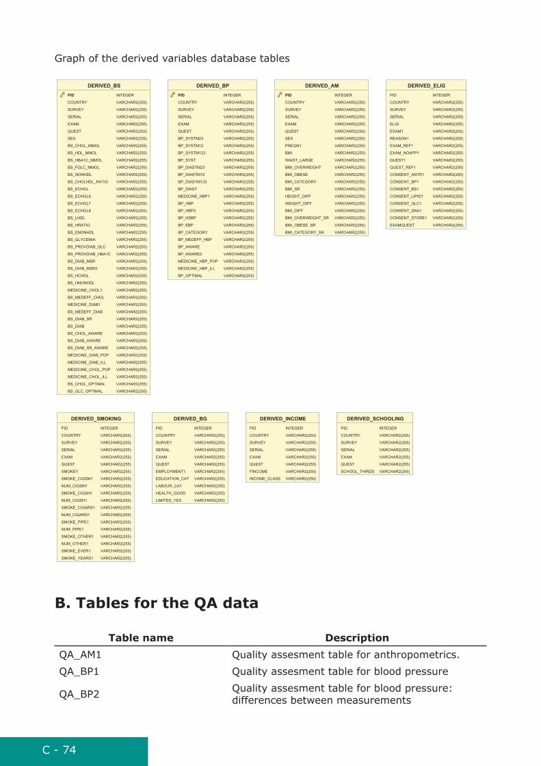
C - 74

Graph of the derived variables database tables

DERIVED_AM

PID INTEGER

COUNTRY VARCHAR2(255)

SURVEY VARCHAR2(255)

SERIAL VARCHAR2(255)

EXAM VARCHAR2(255)

QUEST VARCHAR2(255)

SEX VARCHAR2(255)

PREGN1 VARCHAR2(255)

BMI VARCHAR2(255)

WAIST_LARGE VARCHAR2(255)

BMI_OVERWEIGHT VARCHAR2(255)

BMI_OBESE VARCHAR2(255)

BMI_CATEGORY VARCHAR2(255)

BMI_SR VARCHAR2(255)

HEIGHT_DIFF VARCHAR2(255)

WEIGHT_DIFF VARCHAR2(255)

BMI_DIFF VARCHAR2(255)

BMI_OVERWEIGHT_SR VARCHAR2(255)

BMI_OBESE_SR VARCHAR2(255)

BMI_CATEGORY_SR VARCHAR2(255)

DERIVED_BG

PID INTEGER




EXAM VARCHAR2(255)

QUEST VARCHAR2(255)

EMPLOYMENT1 VARCHAR2(255)

EDUCATION_CAT VARCHAR2(255)

LABOUR_CAT VARCHAR2(255)

HEALTH_GOOD VARCHAR2(255)

LIMITED_YES VARCHAR2(255)

DERIVED_BP

PID INTEGER




EXAM VARCHAR2(255)

QUEST VARCHAR2(255)

BP_SYSTM23 VARCHAR2(255)



BP_SYST VARCHAR2(255)

BP_DIASTM23 VARCHAR2(255)



BP_DIAST VARCHAR2(255)

MEDICINE_HBP1 VARCHAR2(255)

BP_HBP VARCHAR2(255)

BP_HBP2 VARCHAR2(255)

BP_HSBP VARCHAR2(255)

BP_EBP VARCHAR2(255)

BP_CATEGORY VARCHAR2(255)

BP_MEDEFF_HBP VARCHAR2(255)

BP_AWARE VARCHAR2(255)

BP_AWARE2 VARCHAR2(255)

MEDICINE_HBP_POP VARCHAR2(255)

MEDICINE_HBP_ILL VARCHAR2(255)

BP_OPTIMAL VARCHAR2(255)

DERIVED_BS

PID INTEGER




EXAM VARCHAR2(255)

QUEST VARCHAR2(255)

SEX VARCHAR2(255)

BS_CHOL_MMOL VARCHAR2(255)

BS_HDL_MMOL VARCHAR2(255)

BS_HBA1C_MMOL VARCHAR2(255)

BS_FGLC_MMOL VARCHAR2(255)

BS_NONHDL VARCHAR2(255)

BS_CHOLHDL_RATIO VARCHAR2(255)

BS_ECHOL VARCHAR2(255)

BS_ECHOL6 VARCHAR2(255)



BS_LHDL VARCHAR2(255)

BS_HRATIO VARCHAR2(255)

BS_ENONHDL VARCHAR2(255)

BS_GLYCEMIA VARCHAR2(255)

BS_PROVDIAB_GLC VARCHAR2(255)

BS_PROVDIAB_HBA1C VARCHAR2(255)

BS_DIAB_MSR VARCHAR2(255)

BS_DIAB_MSR2 VARCHAR2(255)

BS_HCHOL VARCHAR2(255)

BS_HNONHDL VARCHAR2(255)

MEDICINE_CHOL1 VARCHAR2(255)

BS_MEDEFF_CHOL VARCHAR2(255)

MEDICINE_DIAB1 VARCHAR2(255)

BS_MEDEFF_DIAB VARCHAR2(255)

BS_DIAB_SR VARCHAR2(255)

BS_DIAB VARCHAR2(255)

BS_CHOL_AWARE VARCHAR2(255)

BS_DIAB_AWARE VARCHAR2(255)

BS_DIAB_SR_AWARE VARCHAR2(255)

MEDICINE_DIAB_POP VARCHAR2(255)

MEDICINE_DIAB_ILL VARCHAR2(255)

MEDICINE_CHOL_POP VARCHAR2(255)

MEDICINE_CHOL_ILL VARCHAR2(255)

BS_CHOL_OPTIMAL VARCHAR2(255)

BS_GLC_OPTIMAL VARCHAR2(255)

DERIVED_ELIG

PID INTEGER




ELIG VARCHAR2(255)

EXAM1 VARCHAR2(255)

REASON1 VARCHAR2(255)

EXAM_REF1 VARCHAR2(255)

EXAM_NOAPP1 VARCHAR2(255)

QUEST1 VARCHAR2(255)

QUEST_REF1 VARCHAR2(255)

CONSENT_ANTR1 VARCHAR2(255)

CONSENT_BP1 VARCHAR2(255)

CONSENT_BS1 VARCHAR2(255)

CONSENT_LIPID1 VARCHAR2(255)

CONSENT_GLC1 VARCHAR2(255)

CONSENT_DNA1 VARCHAR2(255)

CONSENT_STORE1 VARCHAR2(255)

EXAMQUEST VARCHAR2(255)

DERIVED_INCOME

PID INTEGER




EXAM VARCHAR2(255)

QUEST VARCHAR2(255)

FINCOME VARCHAR2(255)

INCOME_CLASS VARCHAR2(255)

DERIVED_SCHOOLING

PID INTEGER




EXAM VARCHAR2(255)

QUEST VARCHAR2(255)

SCHOOL_THIRDS VARCHAR2(255)

DERIVED_SMOKING

PID INTEGER




EXAM VARCHAR2(255)

QUEST VARCHAR2(255)

SMOKEY VARCHAR2(255)

SMOKE_CIGSM1 VARCHAR2(255)

NUM_CIGSM1 VARCHAR2(255)

SMOKE_CIGSH1 VARCHAR2(255)

NUM_CIGSH1 VARCHAR2(255)

SMOKE_CIGARS1 VARCHAR2(255)

NUM_CIGARS1 VARCHAR2(255)

SMOKE_PIPE1 VARCHAR2(255)

NUM_PIPE1 VARCHAR2(255)

SMOKE_OTHER1 VARCHAR2(255)

NUM_OTHER1 VARCHAR2(255)

SMOKE_EVER1 VARCHAR2(255)

SMOKE_YEARS1 VARCHAR2(255)

b. tables for the Qa data

table name Description QA_AM1 Quality assesment table for anthropometrics. QA_BP1 Quality assesment table for blood pressure

QA_BP2 Quality assesment table for blood pressure: differences between measurements

C - 75


QA_BS1 Quality assesment table for blood samples

QA_DIST_AM_CAT Quality assesment table for anthropometric data: distribution of continuous variables

QA_DIST_AM_CONT Quality assesment table for anthropometric data: distribution of continuous variables

QA_DIST_BG_CAT Quality assesment table for background and heath status data: distribution of categorical variables

QA_DIST_BG_CONT Quality assesment table for background and heath status data: distribution of continuous variables

QA_DIST_BP_CAT Quality assesment table for anthropometric data: distribution of categorical variables

QA_DIST_BP_CONT Quality assesment table for blood pressure measurement data: distribution of continuous variables

QA_DIST_ELIGIBILITY_CAT Quality assesment table for eligibility data: distribution of categorical variables

QA_DIST_ELIGIBILITY_CONT Quality assesment table for eligibility data: distribution of continuous variables

QA_DIST_LABORATORY_CAT Quality assesment table for laboratory data: distribution of categorical variables

QA_DIST_LABORATORY_CONT Quality assesment table for laboratory data: distribution of continuous variables

QA_DIST_SAMPLING_CAT Quality assesment table for sampling data: distribution of categorical variables

QA_DIST_SAMPLING_CONT Quality assesment table for sampling data: distribution of continuous variables

QA_DIST_SMOKING_CAT Quality assesment table for smoking data: distribution of categorical variables

QA_DIST_SMOKING_CONT Quality assesment table for smoking data: distribution of continuous variables

QA_ELIGIBLES Quality assesment table: Proportions of eligibility data by sex and age group.

QA_MEANS Quality assesment table: Non-weighted means by sex and age group.

QA_PR Participation rates.

QA_PR2 Sex and age distribution of participants and non-participants

QA_PREVALENCES Quality assesment table: Prevalences by sex and age group (non-weighted).

QA_QUEST Quality assesment table for questionnaire QA_SAMPLING1 Quality assesment table for sampling.

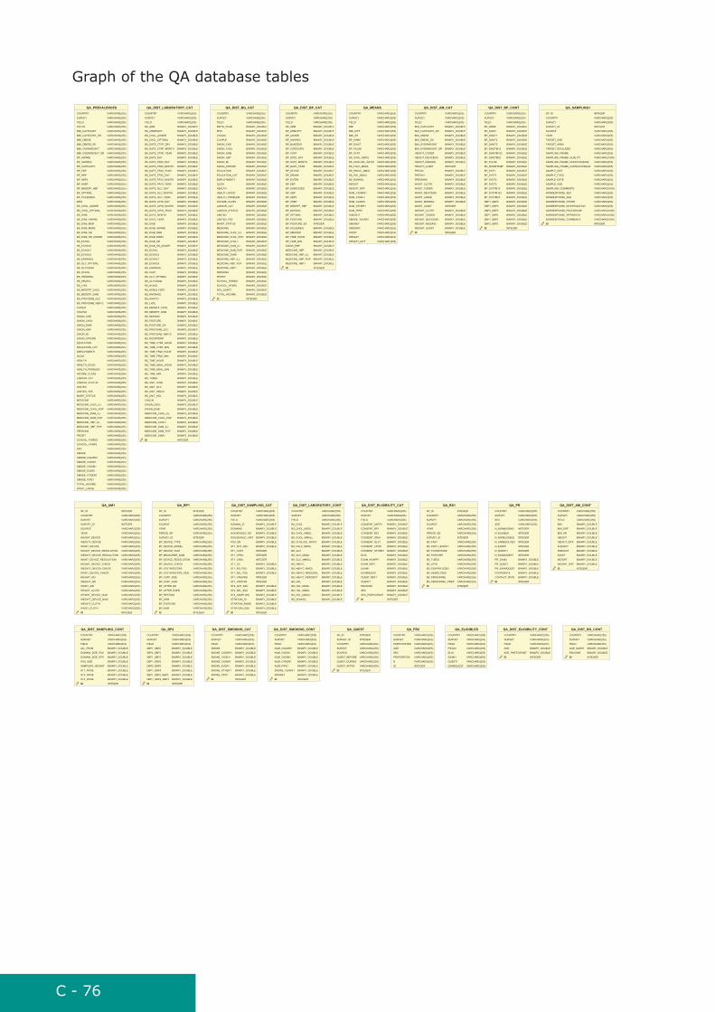
C - 76

Graph of the QA database tables

QA_AM1

SP_ID INTEGER



SURVEY_ID INTEGER

SOURCE VARCHAR2(255)

YEAR VARCHAR2(255)

HEIGHT_DEVICE VARCHAR2(255)

WEIGHT_DEVICE VARCHAR2(255)

WAIST_DEVICE VARCHAR2(255)

HEIGHT_DEVICE_RESOLUTION VARCHAR2(255)

WEIGHT_DEVICE_RESOLUTION VARCHAR2(255)

WAIST_DEVICE_RESOLUTION VARCHAR2(255)

HEIGHT_DEVICE_CHECK VARCHAR2(255)

WEIGHT_DEVICE_CHECK VARCHAR2(255)

WAIST_DEVICE_CHECK VARCHAR2(255)

HEIGHT_AID VARCHAR2(255)

WEIGHT_AID VARCHAR2(255)

WAIST_AID VARCHAR2(255)

HEIGHT_CLOTH VARCHAR2(255)

HEIGHT_DEVICE_NUM VARCHAR2(255)

WEIGHT_DEVICE_NUM VARCHAR2(255)

WEIGHT_CLOTH VARCHAR2(255)

WAIST_CLOTH VARCHAR2(255)

ID INTEGER

QA_BP1

SP_ID INTEGER




YEAR VARCHAR2(255)

PERIOD_BP VARCHAR2(255)

SURVEY_ID INTEGER

BP_DEVICE_TYPE VARCHAR2(255)

BP_DEVICE_MODEL VARCHAR2(255)

BP_DEVICE_NUM VARCHAR2(255)

BP_MEASURER_NUM VARCHAR2(255)

BP_DEVICE_RESOLUTION VARCHAR2(255)

BP_DEVICE_CHECK VARCHAR2(255)

BP_STETHOSCOPE VARCHAR2(255)

BP_STETHOSCOPE_SIDE VARCHAR2(255)

BP_CUFF_SIZE VARCHAR2(255)

BP_CUFF_NUM VARCHAR2(255)

BP_AFTER_BS VARCHAR2(255)

BP_AFTER_EXER VARCHAR2(255)

BP_RESTING VARCHAR2(255)

BP_ARM VARCHAR2(255)

BP_POSTURE VARCHAR2(255)

BP_NUM VARCHAR2(255)

ID INTEGER

QA_BP2COUNTRY VARCHAR2(255)


FIELD VARCHAR2(255)

SBP1_SBP2 BINARY_DOUBLE



DBP1_DBP2 BINARY_DOUBLE



SBP1_SBP2_SBP3 BINARY_DOUBLE

DBP1_DBP2_DBP3 BINARY_DOUBLE

ID INTEGER

QA_BS1

SP_ID INTEGER




YEAR VARCHAR2(255)

PERIOD_BS VARCHAR2(255)

SURVEY_ID INTEGER

BS_FAST VARCHAR2(255)

BS_FAST_LENGTH VARCHAR2(255)

BS_FOODINTAKE VARCHAR2(255)

BS_POSTURE VARCHAR2(255)

BS_TUBES VARCHAR2(255)

BS_LIPID VARCHAR2(255)

BS_CENTRIFUGED VARCHAR2(255)

BS_HEMOLYSED VARCHAR2(255)

BS_PERSONNEL VARCHAR2(255)

BS_PERSONNEL_PREP VARCHAR2(255)

ID INTEGER

QA_DIST_AM_CATCOUNTRY VARCHAR2(255)


FIELD VARCHAR2(255)

BMI_CATEGORY BINARY_DOUBLE

BMI_CATEGORY_SR BINARY_DOUBLE

BMI_OBESE BINARY_DOUBLE

BMI_OBESE_SR BINARY_DOUBLE

BMI_OVERWEIGHT BINARY_DOUBLE

BMI_OVERWEIGHT_SR BINARY_DOUBLE

HEIGHT_CODER BINARY_DOUBLE

HEIGHT_DEVICENO BINARY_DOUBLE

HEIGHT_MISSING BINARY_DOUBLE

HEIGHT_ULIMIT INTEGER

PREGN BINARY_DOUBLE

PREGN1 BINARY_DOUBLE

PREGNWK BINARY_DOUBLE

WAIST_CLOTH BINARY_DOUBLE

WAIST_CODER BINARY_DOUBLE

WAIST_DEVICENO BINARY_DOUBLE

WAIST_LARGE BINARY_DOUBLE

WAIST_MISSING BINARY_DOUBLE

WAIST_ULIMIT INTEGER

WEIGHT_CLOTH BINARY_DOUBLE

WEIGHT_CODER BINARY_DOUBLE

WEIGHT_DEVICENO BINARY_DOUBLE

WEIGHT_MISSING BINARY_DOUBLE

WEIGHT_ULIMIT BINARY_DOUBLE

ID INTEGER

QA_DIST_AM_CONT



FIELD VARCHAR2(255)

BMI BINARY_DOUBLE

BMI_DIFF BINARY_DOUBLE

BMI_SR BINARY_DOUBLE

HEIGHT BINARY_DOUBLE

HEIGHT_DIFF BINARY_DOUBLE

SHEIGHT BINARY_DOUBLE

SWEIGHT BINARY_DOUBLE

WAIST BINARY_DOUBLE

WEIGHT BINARY_DOUBLE

WEIGHT_DIFF BINARY_DOUBLE

ID INTEGER

QA_DIST_BG_CATCOUNTRY VARCHAR2(255)


FIELD VARCHAR2(255)

BIRTH_YEAR BINARY_DOUBLE

BPM BINARY_DOUBLE

CHOLM BINARY_DOUBLE

COUPLE BINARY_DOUBLE

DIAGN_CHD BINARY_DOUBLE

DIAGN_CHOL BINARY_DOUBLE

DIAGN_DIAB BINARY_DOUBLE

DIAGN_HBP BINARY_DOUBLE

DIAGN_MI BINARY_DOUBLE

DIAGN_STROKE BINARY_DOUBLE

EDUCATION BINARY_DOUBLE

EDUCATION_CAT BINARY_DOUBLE

EMPLOYMENT1 BINARY_DOUBLE

GLCM BINARY_DOUBLE

HEALTH BINARY_DOUBLE

HEALTH_GOOD BINARY_DOUBLE

HEALTH_PROBLEM BINARY_DOUBLE

INCOME_CLASS BINARY_DOUBLE

LABOUR_CAT BINARY_DOUBLE

LABOUR_STATUS BINARY_DOUBLE

LIMITED BINARY_DOUBLE

LIMITED_YES BINARY_DOUBLE

MARIT_STATUS BINARY_DOUBLE

MEDICINE BINARY_DOUBLE

MEDICINE_CHOL_ILL BINARY_DOUBLE

MEDICINE_CHOL_POP BINARY_DOUBLE

MEDICINE_CHOL1 BINARY_DOUBLE

MEDICINE_DIAB_ILL BINARY_DOUBLE

MEDICINE_DIAB_POP BINARY_DOUBLE

MEDICINE_DIAB1 BINARY_DOUBLE

MEDICINE_HBP_ILL BINARY_DOUBLE

MEDICINE_HBP_POP BINARY_DOUBLE

MEDICINE_HBP1 BINARY_DOUBLE

PERSONS BINARY_DOUBLE

PROFIT BINARY_DOUBLE

SCHOOL_THIRDS BINARY_DOUBLE

SCHOOL_YEARS BINARY_DOUBLE

SEX_QUEST BINARY_DOUBLE

TOTAL_INCOME BINARY_DOUBLE

ID INTEGER

QA_DIST_BG_CONTCOUNTRY VARCHAR2(255)


FIELD VARCHAR2(255)

AGE_QUEST BINARY_DOUBLE

FINCOME BINARY_DOUBLE

ID INTEGER

QA_DIST_BP_CATCOUNTRY VARCHAR2(255)


FIELD VARCHAR2(255)

BP_ARM BINARY_DOUBLE

BP_ARMLEFT BINARY_DOUBLE

BP_AWARE BINARY_DOUBLE

BP_AWARE2 BINARY_DOUBLE

BP_BLADDER BINARY_DOUBLE

BP_CATEGORY BINARY_DOUBLE

BP_CUFF BINARY_DOUBLE

BP_DATE_DAY BINARY_DOUBLE

BP_DATE_MONTH BINARY_DOUBLE

BP_DATE_YEAR BINARY_DOUBLE

BP_DEVICE BINARY_DOUBLE

BP_DRANK BINARY_DOUBLE

BP_EATEN BINARY_DOUBLE

BP_EBP BINARY_DOUBLE

BP_EXERCISED BINARY_DOUBLE

BP_HBP BINARY_DOUBLE

BP_HBP2 BINARY_DOUBLE

BP_HSBP BINARY_DOUBLE

BP_MEDEFF_HBP BINARY_DOUBLE

BP_MISSING BINARY_DOUBLE

BP_OPTIMAL BINARY_DOUBLE

BP_POSTURE BINARY_DOUBLE

BP_POSTURE_EX INTEGER

BP_PULSEREG BINARY_DOUBLE

BP_SMOKED BINARY_DOUBLE

BP_TIME_HOUR BINARY_DOUBLE

BP_TIME_MIN BINARY_DOUBLE

DIAGN_HBP BINARY_DOUBLE

MEDICINE_HBP BINARY_DOUBLE

MEDICINE_HBP_ILL BINARY_DOUBLE

MEDICINE_HBP_POP BINARY_DOUBLE

MEDICINE_HBP1 BINARY_DOUBLE

ID INTEGER

QA_DIST_BP_CONTCOUNTRY VARCHAR2(255)


FIELD VARCHAR2(255)

BP_ARMC BINARY_DOUBLE

BP_DIAST BINARY_DOUBLE

BP_DIAST1 BINARY_DOUBLE



BP_DIASTM12 BINARY_DOUBLE



BP_PULSE BINARY_DOUBLE

BP_ROOMTEMP BINARY_DOUBLE

BP_SYST BINARY_DOUBLE

BP_SYST1 BINARY_DOUBLE



BP_SYSTM12 BINARY_DOUBLE









ID INTEGER

QA_DIST_ELIGIBILITY_CAT



FIELD VARCHAR2(255)

CONSENT_ANTR1 BINARY_DOUBLE

CONSENT_BP1 BINARY_DOUBLE

CONSENT_BS1 BINARY_DOUBLE

CONSENT_DNA1 BINARY_DOUBLE

CONSENT_GLC1 BINARY_DOUBLE

CONSENT_LIPID1 BINARY_DOUBLE

CONSENT_STORE1 BINARY_DOUBLE

ELIG BINARY_DOUBLE

EXAM_NOAPP1 BINARY_DOUBLE

EXAM_REF1 BINARY_DOUBLE

EXAM1 BINARY_DOUBLE

EXAMQUEST BINARY_DOUBLE

QUEST_REF1 BINARY_DOUBLE

QUEST1 BINARY_DOUBLE

REASON1 BINARY_DOUBLE

SEX BINARY_DOUBLE

SEX_PARTICIPANT BINARY_DOUBLE

ID INTEGER

QA_DIST_ELIGIBILITY_CONTCOUNTRY VARCHAR2(255)


FIELD VARCHAR2(255)

AGE BINARY_DOUBLE

AGE_PARTICIPANT BINARY_DOUBLE

ID INTEGER

QA_DIST_LABORATORY_CATCOUNTRY VARCHAR2(255)


FIELD VARCHAR2(255)

BS_ARM BINARY_DOUBLE

BS_ARMRIGHT BINARY_DOUBLE

BS_CHOL_AWARE BINARY_DOUBLE

BS_CHOL_OPTIMAL BINARY_DOUBLE

BS_DATE_CTRF_DAY BINARY_DOUBLE

BS_DATE_CTRF_MONTH BINARY_DOUBLE

BS_DATE_CTRF_YEAR BINARY_DOUBLE

BS_DATE_DAY BINARY_DOUBLE

BS_DATE_FR20_DAY BINARY_DOUBLE

BS_DATE_FR20_MONTH BINARY_DOUBLE

BS_DATE_FR20_YEAR BINARY_DOUBLE

BS_DATE_FR70_DAY BINARY_DOUBLE

BS_DATE_FR70_MONTH BINARY_DOUBLE

BS_DATE_FR70_YEAR BINARY_DOUBLE

BS_DATE_GLC_DAY BINARY_DOUBLE

BS_DATE_GLC_MONTH BINARY_DOUBLE

BS_DATE_GLC_YEAR BINARY_DOUBLE

BS_DATE_LIPID_DAY BINARY_DOUBLE

BS_DATE_LIPID_MONTH BINARY_DOUBLE

BS_DATE_LIPID_YEAR BINARY_DOUBLE

BS_DATE_MONTH BINARY_DOUBLE

BS_DATE_YEAR BINARY_DOUBLE

BS_DIAB BINARY_DOUBLE

BS_DIAB_AWARE BINARY_DOUBLE

BS_DIAB_MSR BINARY_DOUBLE

BS_DIAB_MSR2 BINARY_DOUBLE

BS_DIAB_SR BINARY_DOUBLE

BS_DIAB_SR_AWARE BINARY_DOUBLE

BS_ECHOL BINARY_DOUBLE

BS_ECHOL6 BINARY_DOUBLE



BS_ENONHDL BINARY_DOUBLE

BS_FAST BINARY_DOUBLE

BS_GLC_OPTIMAL BINARY_DOUBLE

BS_GLYCEMIA BINARY_DOUBLE

BS_HCHOL BINARY_DOUBLE

BS_HEMOLYSED BINARY_DOUBLE

BS_HNONHDL BINARY_DOUBLE

BS_HRATIO BINARY_DOUBLE

BS_LHDL BINARY_DOUBLE

BS_MEDEFF_CHOL BINARY_DOUBLE

BS_MEDEFF_DIAB BINARY_DOUBLE

BS_MISSING BINARY_DOUBLE

BS_POSTURE BINARY_DOUBLE

BS_POSTURE_EX BINARY_DOUBLE

BS_PROVDIAB_GLC BINARY_DOUBLE

BS_PROVDIAB_HBA1C BINARY_DOUBLE

BS_ROOMTEMP BINARY_DOUBLE

BS_TIME_CTRF_HOUR BINARY_DOUBLE

BS_TIME_CTRF_MIN BINARY_DOUBLE

BS_TIME_FR20_HOUR BINARY_DOUBLE

BS_TIME_FR20_MIN BINARY_DOUBLE

BS_TIME_HOUR BINARY_DOUBLE

BS_TIME_MEAL_HOUR BINARY_DOUBLE

BS_TIME_MEAL_MIN BINARY_DOUBLE

BS_TIME_MIN BINARY_DOUBLE

BS_TUBES BINARY_DOUBLE

BS_UNIT_CHOL BINARY_DOUBLE

BS_UNIT_GLC BINARY_DOUBLE

BS_UNIT_HBA1C BINARY_DOUBLE

BS_UNIT_HDL BINARY_DOUBLE

CHOLM BINARY_DOUBLE

DIAGN_CHOL BINARY_DOUBLE

DIAGN_DIAB BINARY_DOUBLE

MEDICINE_CHOL_ILL BINARY_DOUBLE

MEDICINE_CHOL_POP BINARY_DOUBLE

MEDICINE_CHOL1 BINARY_DOUBLE

MEDICINE_DIAB_ILL BINARY_DOUBLE

MEDICINE_DIAB_POP BINARY_DOUBLE

MEDICINE_DIAB1 BINARY_DOUBLE

ID INTEGER

QA_DIST_LABORATORY_CONT



FIELD VARCHAR2(255)

BS_CHOL BINARY_DOUBLE

BS_CHOL_MGDL BINARY_DOUBLE

BS_CHOL_MMOL BINARY_DOUBLE

BS_CHOL_MMOLL BINARY_DOUBLE

BS_CHOLHDL_RATIO BINARY_DOUBLE

BS_FGLC_MMOL BINARY_DOUBLE

BS_GLC BINARY_DOUBLE

BS_GLC_MGDL BINARY_DOUBLE

BS_GLC_MMOLL BINARY_DOUBLE

BS_HBA1C BINARY_DOUBLE

BS_HBA1C_MMOL BINARY_DOUBLE

BS_HBA1C_MMOLMOL BINARY_DOUBLE

BS_HBA1C_PERCENT BINARY_DOUBLE

BS_HDL BINARY_DOUBLE

BS_HDL_MGDL BINARY_DOUBLE

BS_HDL_MMOL BINARY_DOUBLE

BS_HDL_MMOLL BINARY_DOUBLE

BS_NONHDL BINARY_DOUBLE

QA_DIST_SAMPLING_CAT



FIELD VARCHAR2(255)

DOMAIN_ID BINARY_DOUBLE

DOMAINS BINARY_DOUBLE

HOUSEHOLD_SN BINARY_DOUBLE

HOUSEHOLD_UNIT BINARY_DOUBLE

PSU_SN BINARY_DOUBLE

ST1_ANT_SSU BINARY_DOUBLE

ST1_COST INTEGER

ST1_CPSU INTEGER

ST1_CSSU INTEGER

ST1_CV BINARY_DOUBLE

ST1_NO_PSU BINARY_DOUBLE

ST1_SEL_PSU BINARY_DOUBLE

ST1_VAMONG INTEGER

ST1_VWITHIN INTEGER

ST2_ANT_SSU BINARY_DOUBLE

ST2_SEL_SSU BINARY_DOUBLE

ST3_SAMPLING BINARY_DOUBLE

STRATUM_ID BINARY_DOUBLE

STRATUM_NAME BINARY_DOUBLE

STRATUM_SIZE BINARY_DOUBLE

ID INTEGER

QA_DIST_SAMPLING_CONTCOUNTRY VARCHAR2(255)


FIELD VARCHAR2(255)

ALL_PROB BINARY_DOUBLE

DOMAIN_SIZE_PSU BINARY_DOUBLE

DOMAIN_SIZE_STR BINARY_DOUBLE

PSU_SIZE BINARY_DOUBLE

SAMPLING_WEIGHT BINARY_DOUBLE

ST1_PROB BINARY_DOUBLE



ID INTEGER

QA_DIST_SMOKING_CATCOUNTRY VARCHAR2(255)


FIELD VARCHAR2(255)

SMOKE BINARY_DOUBLE

SMOKE_CIGARS1 BINARY_DOUBLE

SMOKE_CIGSH1 BINARY_DOUBLE

SMOKE_CIGSM1 BINARY_DOUBLE

SMOKE_EVER1 BINARY_DOUBLE

SMOKE_OTHER1 BINARY_DOUBLE

SMOKE_PIPE1 BINARY_DOUBLE

ID INTEGER

QA_DIST_SMOKING_CONTCOUNTRY VARCHAR2(255)


FIELD VARCHAR2(255)

NUM_CIGARS1 BINARY_DOUBLE

NUM_CIGSH1 BINARY_DOUBLE

NUM_CIGSM1 BINARY_DOUBLE

NUM_OTHER1 BINARY_DOUBLE

NUM_PIPE1 BINARY_DOUBLE

SMOKE_YEARS1 BINARY_DOUBLE

SMOKEY BINARY_DOUBLE

ID INTEGER

QA_ELIGIBLESCOUNTRY VARCHAR2(255)


FIELD VARCHAR2(255)

FIELD2 VARCHAR2(255)

ELIG VARCHAR2(255)

EXAM1 VARCHAR2(255)

QUEST1 VARCHAR2(255)

EXAMQUEST VARCHAR2(255)

QA_MEANSCOUNTRY VARCHAR2(255)


FIELD VARCHAR2(255)

BMI VARCHAR2(255)

BMI_DIFF VARCHAR2(255)

BMI_SR VARCHAR2(255)

BP_ARMC VARCHAR2(255)

BP_DIAST VARCHAR2(255)

BP_PULSE VARCHAR2(255)

BP_SYST VARCHAR2(255)

BS_CHOL_MMOL VARCHAR2(255)

BS_CHOLHDL_RATIO VARCHAR2(255)

BS_FGLC_MMOL VARCHAR2(255)

BS_HBA1C_MMOL VARCHAR2(255)

BS_HDL_MMOL VARCHAR2(255)

BS_NONHDL VARCHAR2(255)

HEIGHT VARCHAR2(255)

HEIGHT_DIFF VARCHAR2(255)

NUM_CIGARS1 VARCHAR2(255)

NUM_CIGSH1 VARCHAR2(255)

NUM_CIGSM1 VARCHAR2(255)

NUM_OTHER1 VARCHAR2(255)

NUM_PIPE1 VARCHAR2(255)

SHEIGHT VARCHAR2(255)

SMOKE_YEARS1 VARCHAR2(255)

SMOKEY VARCHAR2(255)

SWEIGHT VARCHAR2(255)

WAIST VARCHAR2(255)

WEIGHT VARCHAR2(255)

WEIGHT_DIFF VARCHAR2(255)

QA_PR



SEX VARCHAR2(255)

AGE VARCHAR2(255)

N_NONMISSING INTEGER

N_ELIGIBLE INTEGER

N_NONELIGIBLE INTEGER

N_UNRESOLVED INTEGER

N_EXAM1 INTEGER

N_QUEST1 INTEGER

N_EXAMQUEST INTEGER

PR_EXAM BINARY_DOUBLE

PR_QUEST BINARY_DOUBLE

PR_EXAMQUEST BINARY_DOUBLE

COOPERATE BINARY_DOUBLE

CONTACT_RATE BINARY_DOUBLE

ID INTEGER

QA_PR2COUNTRY VARCHAR2(255)


PARTICIPATED VARCHAR2(255)

AGE VARCHAR2(255)

SEX VARCHAR2(255)

PROPORTION VARCHAR2(255)

N VARCHAR2(255)

ID INTEGER

QA_PREVALENCESCOUNTRY VARCHAR2(255)


FIELD VARCHAR2(255)

FIELD2 VARCHAR2(255)

BMI_CATEGORY VARCHAR2(255)

BMI_CATEGORY_SR VARCHAR2(255)

BMI_OBESE VARCHAR2(255)

BMI_OBESE_SR VARCHAR2(255)

BMI_OVERWEIGHT VARCHAR2(255)

BMI_OVERWEIGHT_SR VARCHAR2(255)

BP_AWARE VARCHAR2(255)

BP_AWARE2 VARCHAR2(255)

BP_CATEGORY VARCHAR2(255)

BP_EBP VARCHAR2(255)

BP_HBP VARCHAR2(255)

BP_HBP2 VARCHAR2(255)

BP_HSBP VARCHAR2(255)

BP_MEDEFF_HBP VARCHAR2(255)

BP_OPTIMAL VARCHAR2(255)

BP_PULSEREG VARCHAR2(255)

BPM VARCHAR2(255)

BS_CHOL_AWARE VARCHAR2(255)

BS_CHOL_OPTIMAL VARCHAR2(255)

BS_DIAB VARCHAR2(255)

BS_DIAB_AWARE VARCHAR2(255)

BS_DIAB_MSR VARCHAR2(255)

BS_DIAB_MSR2 VARCHAR2(255)

BS_DIAB_SR VARCHAR2(255)

BS_DIAB_SR_AWARE VARCHAR2(255)

BS_ECHOL VARCHAR2(255)




BS_ENONHDL VARCHAR2(255)

BS_GLC_OPTIMAL VARCHAR2(255)

BS_GLYCEMIA VARCHAR2(255)

BS_HCHOL VARCHAR2(255)

BS_HNONHDL VARCHAR2(255)

BS_HRATIO VARCHAR2(255)

BS_LHDL VARCHAR2(255)

BS_MEDEFF_CHOL VARCHAR2(255)

BS_MEDEFF_DIAB VARCHAR2(255)

BS_PROVDIAB_GLC VARCHAR2(255)

BS_PROVDIAB_HBA1C VARCHAR2(255)

CHOLM VARCHAR2(255)

COUPLE VARCHAR2(255)

DIAGN_CHD VARCHAR2(255)

DIAGN_CHOL VARCHAR2(255)

DIAGN_DIAB VARCHAR2(255)

DIAGN_HBP VARCHAR2(255)

DIAGN_MI VARCHAR2(255)

DIAGN_STROKE VARCHAR2(255)

EDUCATION VARCHAR2(255)

EDUCATION_CAT VARCHAR2(255)

EMPLOYMENT1 VARCHAR2(255)

GLCM VARCHAR2(255)

HEALTH VARCHAR2(255)

HEALTH_GOOD VARCHAR2(255)

HEALTH_PROBLEM VARCHAR2(255)

INCOME_CLASS VARCHAR2(255)

LABOUR_CAT VARCHAR2(255)

LABOUR_STATUS VARCHAR2(255)

LIMITED VARCHAR2(255)

LIMITED_YES VARCHAR2(255)

MARIT_STATUS VARCHAR2(255)

MEDICINE VARCHAR2(255)

MEDICINE_CHOL_ILL VARCHAR2(255)

MEDICINE_CHOL_POP VARCHAR2(255)

MEDICINE_DIAB_ILL VARCHAR2(255)

MEDICINE_DIAB_POP VARCHAR2(255)

MEDICINE_HBP_ILL VARCHAR2(255)

MEDICINE_HBP_POP VARCHAR2(255)

PERSONS VARCHAR2(255)

PROFIT VARCHAR2(255)

SCHOOL_THIRDS VARCHAR2(255)

SCHOOL_YEARS VARCHAR2(255)

SEX VARCHAR2(255)

SMOKE VARCHAR2(255)

SMOKE_CIGARS1 VARCHAR2(255)

SMOKE_CIGSH1 VARCHAR2(255)

SMOKE_CIGSM1 VARCHAR2(255)

SMOKE_EVER1 VARCHAR2(255)

SMOKE_OTHER1 VARCHAR2(255)

SMOKE_PIPE1 VARCHAR2(255)

TOTAL_INCOME VARCHAR2(255)

WAIST_LARGE VARCHAR2(255)

QA_QUESTSP_ID INTEGER

SURVEY_ID INTEGER




QUEST_BEFORE VARCHAR2(255)

QUEST_DURING VARCHAR2(255)

QUEST_AFTER VARCHAR2(255)

ID INTEGER

QA_SAMPLING1SP_ID INTEGER



SURVEY_ID INTEGER


YEAR VARCHAR2(255)

TARGET_AGE VARCHAR2(255)

TARGET_AREA VARCHAR2(500)

TARGET_EXCLUDED VARCHAR2(500)

SAMPLING_FRAME VARCHAR2(255)

SAMPLING_FRAME_QUALITY VARCHAR2(1000)

SAMPLING_FRAME_NONCOVERAGE VARCHAR2(255)

SAMPLING_FRAME_OVERCOVERAGE VARCHAR2(255)

SAMPLE_SIZE VARCHAR2(255)

SAMPLE_FILES VARCHAR2(255)

SAMPLE_DATE VARCHAR2(255)

SAMPLE_AGE VARCHAR2(255)

SAMPLING_COMMENTS VARCHAR2(1000)

NONRESPONSE_SEX VARCHAR2(255)

NONRESPONSE_AGE VARCHAR2(255)

NONRESPONSE_OTHER VARCHAR2(255)

NONRESPONSE_INVESTIGATION VARCHAR2(255)

NONRESPONSE_PROCEDURE VARCHAR2(1000)

NONRESPONSE_APPROACH VARCHAR2(1000)

NONRESPONSE_COMMENTS VARCHAR2(1000)

ID INTEGER

Part C


C - 77


Evaluation of the national HESs and quality of the data collected by them, includes several steps:

1. National level evaluation through evaluation report2. European level evaluation through

• Site visits• Evaluation of the national manuals• Quality assessment of the collected data

3.1 national level evaluationEvaluation report should be prepared after the survey is completed. The purpose of the evaluation report is to document experiences gath-ered during the survey process, in planning, preparation, fieldwork, data management and analysis. It should summarize what worked well, what were the major challenges and difficulties, and what was learned when carrying out the survey. There is no need to repeat the information already given in the national HES manual, rather use refer-ences to the national HES manual.

In countries with previous or ongoing national surveys, the evaluation should take into account the extra efforts and challenges met when adjusting existing protocols for European standards.

The evaluation report is targeted to:

• those who will plan and prepare the future survey(s), to point out what needs to be taken into account in the prepa-rations;

• those who will use the survey data; • the EHES network, to share experiences, and• those funding the survey, to assess if the survey was, and

will it be in the future worth the investment.

3. Evaluation and quality assuranceHanna Tolonen1, Päivikki Koponen1, Sanna Ahonen1, Johanna Mäki-Opas1, Ari Haukijärvi1, Tarja Palosaari1, Katri Kilpeläinen1, Kari Kuulasmaa1


C - 78

A template for the evaluation report is given in the Appendix 3a. This template is a check list of issues, which at least should be included to the evaluation report. Questions listed under each topic are examples of issues relating to the topic. If other important issues have been ob-served nationally, it is important to document them as well. The evalu-ation report should include both positive and negative experiences. The template can be freely adapted to better serve national interests or to be in line with the evaluation of previous surveys.

3.2 European level evaluation

3.2.1 Site visits

Site visits are an evaluation tool, during which the members of the EHES Reference Centre observe the field work of the national HES. Site visits are planned to take two days, during which actual measurements are observed with the written consent of the participant and the field work staff. The site visits will be carried out, if adequate resources are available for the EHES RC.

During the evaluation of the field work, following issues are observed:

• How the informed consent is obtained;• How the privacy of the participants is ensured;• How each measurement is conducted: are standardized

measurement protocols followed (including blood drawing and sample processing, as well as collection of interview/questionnaire data);

• How staff members interact and communicate with partici-pants;

• How team members communicate and collaborate with each other;

• How the data protection on the field is ensured;• What kind of devices are used for the measurements;• How often and how the used devices are checked and cali-

brated;• Is the log book about the checked, their outcomes and cali-

bration kept;• How the materials (especially blood samples) are trans-

ferred.

A check list of the topics to be covered during the site visit has been prepared and is available in the Appendix 3b.

Also EHES RC members discuss with local survey organizers about:• Selection of the sampling frame;• Sample size and sampling;• Obtaining ethical approval for the survey;

C - 79

• Obtaining informed consent from survey participants;• Selection of included questionnaire modules and measure-

ments;• Time and resources needed for the planning;• Recruitment of fieldwork personnel:• Training of the survey personnel;• Fieldwork logistics;• Data management and data confidentiality/protection;• National quality control actions, including audit visits;• Recruitment of the survey invitees, including possible use of

incentives and obtained participation rate;• Dissemination plan;• Possibly faced difficulties and success stories (what works

well, what have been the biggest challenges).

A written site visit report is prepared, describing the observations and possible deviations from the EHES protocol.

3.2.2 Evaluation of the national manuals

The evaluation of the national HES manuals includes detailed evalua-tion of how well the national manual corresponds to the EHES Manual. This was done for the Manuals prepared by the EHES pilot partner’s. This is suggested to be a task for the EHES RC, but it is possible only when adequate resources are available. Especially the measurement protocols which should remain identical between all surveys need to be checked, preferably before the training and fieldwork are started. Otherwise, the contents of national manuals are evaluated against the contents of the EHES Manual. A detailed evaluation would require translations of the national manuals.

Topics to be checked are:

• Are all the topics outlined in the EHES Manual included in the national manual

• Sampling• Ethics and informed consent• Data management and security• Training• Recruitment process and related documents• Questionnaire(s)• Measurement protocols• Fieldwork logistics• Coordination of the fieldwork• Safety issues during the fieldwork• Budget and funding

C - 80

• Risk assessment• Publicity and dissemination

To help such evaluation, a template with check list has been prepared. This template is available in the Appendix 3c.

3.2.3 Quality assessment of the survey data

Quality assessment of the survey data quantifies how complete and accurate the collected survey data is.

Data for the core measurements and the core questionnaire items will be assessed with pre-defined criteria. The outcome of the assessment should be published in the evaluation report which is an important document to support the interpretation of the results. Data assessment is an essential step of the survey to obtain high quality data, which will be comparable between countries and in particular over time, so that reliable long-term trends can be calculated from the data in the future.

The survey data is evaluated and documented by EHES Reference Cen-tre (if adequate resources are available). For different data items dif-ferent issues are checked.

For questionnaire items:

• questionnaire comparability, i.e. how well nationally used question(s) correspond to the EHES question(s)

• data extraction, i.e. how well EHES data items are extracted for data transfer from nationally collected data

• proportion of missing data for each questionnaire item• distribution of answer alternatives for each categorical data

item• minimum values, maximum values, 10% percentile, me-

dian, 90% percentile and standard deviation for other data items

For measurements:

• recording form comparability with the EHES recording form• level of measurement protocol details in the national HES

manuals in comparison to the EHES Manual• proportion of missing data• minimum values, maximum values, 10% percentile, medi-

an, 90% percentile and standard deviation• for blood pressure:

• proportion of identical readings between subsequent measurements

• distribution of terminal digits

C - 81

• for anthropometric measurements:• proportion of terminal digits

The system for generating relevant tables and figures for evaluation reports was programmed using R, a free software environment for sta-tistical computing and graphics (R 2011). The data assessment re-sults are saved in the Derived Variables and QA Database (see Part C, Chapter 2) in a format that allows the use of different programs and systems for representing and combining the results. Program codes for generating quality assessment tables and figures of the survey data can be found in the Appendix 3d.

references• R Development Core Team (2011). R: A language and environment for

statistical computing. R Foundation for Statistical Computing, Vienna, Aus-tria. ISBN 3-900051-07-0, URL http://www.R-project.org/

C - 82

appendix 3a. template for the nation-al evaluation reportintroduction

• To which survey this evaluation report refers to?• Who prepared and took part in the evaluation (internal, i.e.

within the national survey organization and/or external, i.e. by people independent of the national survey organization)?

• How was the evaluation carried out (e.g. informal discus-sions, feed-back sessions, workshops, meetings, observa-tions)?

Planning and preparation of the survey

• Personnel• Did you have enough personnel to plan and prepare the

survey?• Were there any changes (turnover) in key personnel in-

volved in the planning and preparation?• Did the personnel have all the required expertise?• If you did not have enough personnel or they were lack-

ing some expertise, how did you solve these shortcom-ings?

• Time• Was there enough time for planning, preparations and

fund raising before the actual survey fieldwork started?• If not, how did you solve the situation?

• Management and coordination• Was there adequate collaboration between internal per-

sonnel and other institutes involved in the survey plan-ning and preparation?

• Was the management structure and coordination ade-quately specified and functional?

• Experiences in using management tools?• lessons learned: What worked well in the planning and

preparation phase, what were the major challenges and dif-ficulties, and what would you change and how for the next survey?

budget

• Were you able to raise adequate funding or were any cuts made to the initial budget?

• How well did your original budget hold at different stages of the survey process?

C - 83

• If your budget did not hold, what where the biggest differ-ences, and how did you solve this?

• lessons learned: What worked well in the budgeting, what were the major challenges and difficulties, and what would you change and how for the next survey?

Sampling

• Was it easy to get information about the available sampling frames, about their quality and access to them, or was the best/most feasible sampling frame previously well known?

• Did you have professional (statistical) help when doing the sample selection?

• Was the timing of the sample selection optimal in relation to starting the fieldwork?

• Did you obtain adequate contact information for the select-ed persons?

• If you had any problems, how did you solve them?• lessons learned: What worked well in the sampling, what

were the major challenges and difficulties, and what would you change and how for the next survey?

Ethical approval

• What were the key steps in your ethical approval process?• Which institutes/committees needed to be consulted?• Did you obtain the ethical approval in time to start the field-

work as planned?• What kind of questions the ethical committee(s) raised?• If you had any problems, how did you solve them?• lessons learned: What worked well in the ethical approval

process, what were the major challenges and difficulties, and what would you change and how for the next survey?

Data management

• Did you have adequate professionals to plan, prepare and set up the data management system at national level?

• What were the key steps in planning, preparing and setting up the data management system?

• Did you have adequate hardware and software resources?• Did your software and hardware function as planned (in-

cluding fieldwork, data entry and data checking)?• If you had any problems, how did you solve them?• lessons learned: What worked well in the data manage-

ment, what were the major challenges and difficulties, and what would you change and how for the next survey?

C - 84

training

• Did you collect any feedback from the trainees, e.g. field-work staff, after the training? If yes what were the key is-sues raised in the feedback?

• Did you train all relevant personnel groups?• Did you have enough time to plan and prepare the training?• Did you have adequate trainers?• Was the length of the training period adequate?• Did the training include all relevant components?• Did you have enough practical training for the measure-

ments?• If you had any problems, how did you solve them?• lessons learned: What worked well in the training, what


Recruitment of fieldwork staff

• Were new persons recruited for the survey fieldwork or did you have previous/permanent personnel?

• Did you have part-time or full-time fieldwork staff? Did this lead to any problems?

• Did you have any problems in recruiting personnel with ad-equate qualifications and expertise?

• Did you have any turnover of personnel during the field-work?

• Were extra persons recruited and trained as substitutes for unexpected absences or sick leaves?

• If you had any problems, how did you solve them?• lessons learned: What worked well in the recruitment of

fieldwork staff, what were the major challenges and diffi-culties, and what would you change and how for the next survey?

Equipment

• Did you have adequate equipment for all measurements?• Were there any problems in purchasing, hiring or leasing

the equipment?• Did you have any problems to get equipment serviced and/

or calibrated?• If you had any problems, how did you solve them?• lessons learned: What worked well with the equipment,

what were the major challenges and difficulties, and what would you change and how for the next survey?

C - 85

recruitment of participants

• What were the key steps in recruiting participants?• If you used incentives, did they raise the willingness to par-

ticipate? Were the incentives cost-effective?• Did you change the recruitment method during the field-

work? If yes, why and was it effective?• If you had any problems, how did you solve them?• lessons learned: What worked well in the recruitment of

participants, what were the major challenges and difficul-ties, and what would you change and how for the next sur-vey?

appointment scheduling

• If you used software for appointment scheduling,• How was the program selected/developed?• Did the program work as planned?

• Did you get any feedback from the participants about the available appointment times?

• Did you extend your appointment times during the field-work? If yes, how and was it effective?

• If you had any problems, how did you solve them?• lessons learned: What worked well in the appointment

scheduling, what were the major challenges and difficulties, and what would you change and how for the next survey?

Examination sites

• How did you select your examination sites?• Did the examination sites fulfill all your requirements (pri-

vacy, easy access etc.)?• Was it easy/possible to find suitable examination sites?• If you had any problems, how did you solve them?• lessons learned: What worked well in the the selection of

examination sites, what were the major challenges and dif-ficulties, and what would you change and how for the next survey?

Selection of measurements/questionnaire items

• How did you balance between previous national questions and EHES questions/measurement procedures?

• What were your positive and/or negative experiences from the inclusion of the additional measurements/questionnaire components?

C - 86

• If you had any problems, how did you solve them?• lessons learned: What worked well in the selection of

measurements and questionnaire items, what were the ma-jor challenges and difficulties, and what would you change and how for the next survey?

Questionnaire and recording form design

• Did you find shortcomings (e.g. errors, illogical jump rules, ambiguous questions) in the questionnaire(s) or recording forms?

• Did you get feedback from the participants about the ques-tionnaires? If yes, what kind?

• If you had any problems, how did you solve them?• lessons learned: What worked well in the questionnaire

and recording form design, what were the major challenges and difficulties, and what would you change and how for the next survey?

Quality control

• Did the fieldwork team carry out daily/weekly checking and calibration as planned and record them?

• Were the quality control records monitored regularly?• Were there any audit/control visits additional to the site vis-

its by EHES RC?• If you had any problems, how did you solve them?• lessons learned: What worked well in the quality control,


Data checking

• What kind of errors did you observe during the routine data checking?

• What losses or potential losses of data were observed dur-ing the data inventory?

• If you had any problems, how did you solve them?• lessons learned: What worked well in the data checking,


Feedback to the participants

• Was the feedback to the participant given as planned?• Did the participants consider the feedback and the way how

it was given useful?

C - 87

• If you had any problems, how did you solve them?• lessons learned: What worked well in the feedback to the

participants, what were the major challenges and difficul-ties, and what would you change and how for the next sur-vey?

laboratory

• Were you satisfied with the laboratory?• Did your laboratory participate to the External Quality As-

sessment by EHES RC? If yes, how did the laboratory feel about the assessment and the results?

• If you had any problems, how did you solve them?• lessons learned: What worked well with the laboratory,


Fieldwork coordination and supervision

• Was there sufficient central coordination for the fieldwork (personnel and other resources)?

• Was there adequate supervision and support for the field-work staff?

• If you had any problems, how did you solve them?• lessons learned: What worked well in the fieldwork coor-

dination and supervision, what were the major challenges and difficulties, and what would you change and how for the next survey?

Publicity

• Did you follow a publicity plan and/or organize any media campaigns?

• Did you have professional public relations personnel to help you?

• Were the actions to raise public awareness of your survey effective?

• Was the publicity correctly timed in relation to fieldwork?• If you had any problems, how did you solve them?• lessons learned: What worked well with publicity, what


other aspects of survey

• Were there any other fieldwork practices and aspects that need to be taken into account for the next survey?

C - 88

• If you had any problems, how did you solve them?• lessons learned: What worked well with other aspects of

survey, what were the major challenges and difficulties, and what would you change and how for the next survey?

Summary and conclusions

• Key findings and recommendations for the future.

C - 89

appendix 3b. Contents of the site visitsSampling

Target population

• Geographical area covered• Age group• Permanent residents of the country/citizens/something else• Inclusion of institutionalized (yes/no)

• If yes, which institutions• Other possible limitations to the eligibility (language, etc.)

Sampling frame

• Primary sampling frame• When last updated• Who maintains the sampling frame

• Secondary sampling frame• When last updated• Who maintains the sampling frame

Sample size

• Total sample size• Stratification of the sample size

Sampling method

• Who is responsible for sample selection• Procedure

Survey procedures

Invitation of the participants

• Form of first contact• Max number of contacts• Forms of other contacts• Use of incentives

• Have been used or not• If yes, what kind of

• On which languages

C - 90

Examination site

• Fixed clinic(s)/ mobile clinic/ home/ other• Number of examination sites• Description of the examination site

Questionnaire administration

• On which languages• Self-administered/ interviewed

• Send by post• Filled in at the examination site• Telephone interview (CATI?)• Face-to-face interview (CAPI?)• Combination of above

• Length of the questionnaire (number of questions and pag-es)

• Is questionnaire checked when handed over

Examinations

• Months when examination are conducted• Days of the week when examinations are conducted• Hours during which the examinations are conducted

Blood pressure

• Equipment• BP measurement device (mercury vs. automated)

• Brand and type• Number and size of cuffs• Stethoscope (if mercury); bell or diapgram

• Measurement conditions• Room temperature• Quiet/ noise• Lighting• Adequate table for the measurement device and chair for

the participant

Height measurement

• Equipment• What kind of equipment is used

C - 91

• Does it seem that equipment are used right and the cali-bration is done correctly

• Clothing• Is the height measured without shoes, heavy outer gar-

ments and hair ornaments?• Position during the measurement

• Are back of the head, shoulder blades, buttocks, heels touching the stadiometer/measurement device?

• Is the ear canal in a level with the cheek bone?• If the participant is taller than the measurer, were the steps

used?

Weight measurement


• Does it seem that equipment are used right and the calibra-tion is done correctly

• Participant’s clothing• Is the weight measured in underwear?

Waist circumference


• Participant’s clothing• Is waist measured on bare skin?

• Is the right measurement place palpated?• Are the participants hands hanging beside the body?

C - 92

appendix 3c. national HES manual evaluation templateEvaluation of the national HES manual

During the evaluation process, the following issues are checked:

1. Does the national HES manual cover all the topics listed in the template of the national HES manual, provided by the EHES RC?

2. Are the descriptions under topics written clearly and taking into account the national circumstances?

3. In case the EHES Manual has detailed instructions how the topic, e.g. measurements, should be done, is the EHES rec-ommendations followed so that the comparability of data is ensured?

If the above issues are dealt appropriately, the evaluation form has only a tick mark on ‘Yes’. If there is a tick mark on ‘No’ clarifying comments / questions to those who have prepared the manual are documented.

aims and purpose of the survey Yes no

Is this topic included in the national HES manual? Is the description clear and adapted to the national situation?

Comments:

organization and management of the national HES Yes no


Comments:

timing of the survey Yes no


C - 93

Comments:

target population and sample size

target population Yes no

Is this topic included in the national HES manual? Does the target population correspond to the EHES recommendations?

Is the description clear and adapted to the national situation?

Comments:

Sample size Yes no

Is this topic included in the national HES manual? Does the defined sample size correspond to the EHES recommendations?


Comments:

Sampling procedures

Sampling frame Yes no


Comments:

Sampling procedure Yes no

Is this topic included in the national HES manual? Does the procedure follow the EHES recommendations? Is the description clear and adapted to the national situation?

Comments:

C - 94

Legal, ethical and data confidentiality issues

national legislation and regulations Yes no


Comments:

Process for ethical approval Yes no


Comments:

informed consent form Yes no

Is this topic included in the national HES manual, with a form attached?

Does the informed consent form follow the EHES recommendations?


Comments:

obtaining informed consent Yes no


Comments:

C - 95

recruitment, scheduling appointments and motivating partici-pants

Yes no Is this topic included in the national HES manual? Is the description clear and adapted to the national situation?

Comments:

Quality assurance

training programme Yes no

Is this topic included in the national HES manual? Does the training programme follow the EHES recommendations?


Comments:

Pilot survey Yes no


Comments:

Quality control Yes no

Is this topic included in the national HES manual? Do the quality control procedures follow the EHES recommendations?


Comments:

C - 96

Data management Yes no


Comments:

Selected measurements Yes no

Is this topic included in the national HES manual? Is the description clear and adapted to the national situation, explaining the rationale why each measurement is selected?

Comments:

non-participant information Yes no


Comments:

Selected examination site Yes no


Comments:

Questionnaire and its administration and validation

Questionnaire Yes no

Is this topic included in the national HES manual, with a questionnaire attached?

Does the questionnaire include all the items of the EHES questionnaire?

C - 97


Comments:

Questionnaire administration mode Yes no


Comments:

Checking questionnaires and interviewing Yes no


Comments:

Measurement procedures in the examinations

blood pressure Yes no

Is this topic included in the national HES manual? Do the measurement devices fulfill the EHES requirements?

Does the measurement protocol follow the EHES recommendations?


Comments:

Height Yes no



C - 98


Comments:

Weight Yes no




Comments:

Waist circumference Yes no




Comments:

additional measurements Yes no

Is this topic included in the national HES manual? Are international standards/reference tools followed (if yes, specify these under Comments)?


Comments:

C - 99

Feedback to the participants Yes no


Comments:

analytic laboratory, blood sample collection and storage of the samples

Selection of the analytic laboratory Yes no

It this topic included in the national HES manual? Does the selection criteria correspond to the EHES recommendations?


Comments:

blood sample collection Yes no

Is this topic included in the national HES manual? Do the materials and equipment fulfill the EHES requirements?

Does the sample collection protocol follow the EHES recommendations?


Comments:

Sample logistics Yes no

Is this topic included in the national HES manual? Does the protocol follow the EHES recommendations? Is the description clear and adapted to the national situation?

Comments:

C - 100

long term storage of the samples Yes no

Is this topic included in the national HES manual? Does the protocol follow the EHES recommendations? Is the description clear and adapted to the national situation?

Comments:

Fieldwork staff Yes no

It this topic included in the national HES manual Is the description clear and adapted to the national situation

Comments:

Coordination of the fieldwork Yes no


Comments:

Safety issues during fieldwork Yes no


Comments:

Fieldwork logistics Yes no


Comments:

C - 101

Dissemination, publicity and reporting Yes no


Comments:

budget and funding Yes no


Comments:

risk assessment Yes no


Comments:

Evaluation Yes no


Comments:

C - 102

appendix 3d. Program codes for qual-ity assessmentFollowing R scripts are used in EHES data quality assessment of the survey data.

Database connection is established using R package RODBC (Brian Rip-ley and from 1999 to Oct 2002 Michael Lapsley (2012). RODBC: ODBC Database Access. R package version 1.3-5. http://CRAN.R-project.org/package=RODBC) and SQL (Structured Query Language) is used to import and export data from EHES database.

Program codes use database table variables for the definition of the EHES variables (e.g. code for missing value etc). The definition table variables is of the form:

varnaME Name of the variable

vartYPE Type of variable: Database, Sampling, Eligibility, Questionnaire, Measurement, Laboratory or Derived

DEFinition Definition of the variable and it’s values

ContinuouS 1 if variable is continuous, 0 if variable is categorical

MiSSinG Code for missing value if relevant for variable

DontKnoW Code for value “Don’t know” if relevant for variable

irrElEvant Code for irrelevant value if relevant for variable

EXaM 1 if variable uses information from examination

QuESt 1 if variable uses information from questionnaire

DiviDEr For continuous variables, gives width of x axis for plotting

MiniMuM For continuous variables, gives minimum value of x axis for plotting

MaXiMuM For continuous variables, gives maximum value of x axis for plotting

MEan 1 if continuous and variable is used for indicator calculation

PrEvalEnCE 1 if categorical and variable is used for indicator calculation

r functions for quality assessment of the survey data

drawtable_cat - to derive basic statistics and distribution ta-bles for categorical variables (frequencies, proportion of miss-ing values)

drawtable_cat <- function(data, variables, item=NA) { ### data = dataset, variables = definition table for variables, item = evaluation category # tab, output table tab <- NULL ## to get only categorical variables varnames_cat <- sort(variables$VARNAME[variables$CONTIN

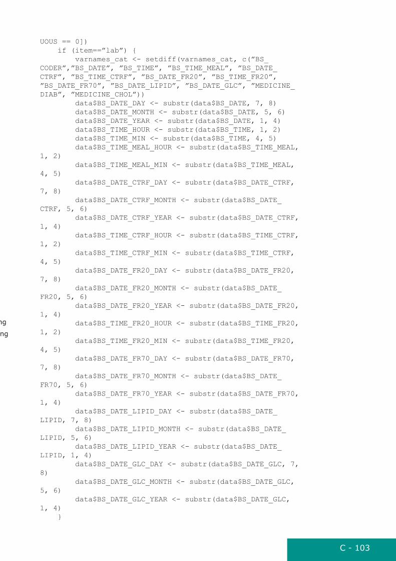
C - 103

UOUS == 0]) if (item==”lab”) { varnames_cat <- setdiff(varnames_cat, c(”BS_CODER”,”BS_DATE”, ”BS_TIME”, ”BS_TIME_MEAL”, ”BS_DATE_CTRF”, ”BS_TIME_CTRF”, ”BS_DATE_FR20”, ”BS_TIME_FR20”, ”BS_DATE_FR70”, ”BS_DATE_LIPID”, ”BS_DATE_GLC”, ”MEDICINE_DIAB”, ”MEDICINE_CHOL”)) data$BS_DATE_DAY <- substr(data$BS_DATE, 7, 8) data$BS_DATE_MONTH <- substr(data$BS_DATE, 5, 6) data$BS_DATE_YEAR <- substr(data$BS_DATE, 1, 4) data$BS_TIME_HOUR <- substr(data$BS_TIME, 1, 2) data$BS_TIME_MIN <- substr(data$BS_TIME, 4, 5) data$BS_TIME_MEAL_HOUR <- substr(data$BS_TIME_MEAL, 1, 2) data$BS_TIME_MEAL_MIN <- substr(data$BS_TIME_MEAL, 4, 5) data$BS_DATE_CTRF_DAY <- substr(data$BS_DATE_CTRF, 7, 8) data$BS_DATE_CTRF_MONTH <- substr(data$BS_DATE_CTRF, 5, 6) data$BS_DATE_CTRF_YEAR <- substr(data$BS_DATE_CTRF, 1, 4) data$BS_TIME_CTRF_HOUR <- substr(data$BS_TIME_CTRF, 1, 2) data$BS_TIME_CTRF_MIN <- substr(data$BS_TIME_CTRF, 4, 5) data$BS_DATE_FR20_DAY <- substr(data$BS_DATE_FR20, 7, 8) data$BS_DATE_FR20_MONTH <- substr(data$BS_DATE_FR20, 5, 6) data$BS_DATE_FR20_YEAR <- substr(data$BS_DATE_FR20, 1, 4) data$BS_TIME_FR20_HOUR <- substr(data$BS_TIME_FR20, 1, 2) data$BS_TIME_FR20_MIN <- substr(data$BS_TIME_FR20, 4, 5) data$BS_DATE_FR70_DAY <- substr(data$BS_DATE_FR70, 7, 8) data$BS_DATE_FR70_MONTH <- substr(data$BS_DATE_FR70, 5, 6) data$BS_DATE_FR70_YEAR <- substr(data$BS_DATE_FR70, 1, 4) data$BS_DATE_LIPID_DAY <- substr(data$BS_DATE_LIPID, 7, 8) data$BS_DATE_LIPID_MONTH <- substr(data$BS_DATE_LIPID, 5, 6) data$BS_DATE_LIPID_YEAR <- substr(data$BS_DATE_LIPID, 1, 4) data$BS_DATE_GLC_DAY <- substr(data$BS_DATE_GLC, 7, 8) data$BS_DATE_GLC_MONTH <- substr(data$BS_DATE_GLC, 5, 6) data$BS_DATE_GLC_YEAR <- substr(data$BS_DATE_GLC, 1, 4) }

appendix 3d. Program codes for qual-ity assessmentFollowing R scripts are used in EHES data quality assessment of the survey data.

Database connection is established using R package RODBC (Brian Rip-ley and from 1999 to Oct 2002 Michael Lapsley (2012). RODBC: ODBC Database Access. R package version 1.3-5. http://CRAN.R-project.org/package=RODBC) and SQL (Structured Query Language) is used to import and export data from EHES database.
















r functions for quality assessment of the survey data

drawtable_cat - to derive basic statistics and distribution ta-bles for categorical variables (frequencies, proportion of miss-ing values)

drawtable_cat <- function(data, variables, item=NA) { ### data = dataset, variables = definition table for variables, item = evaluation category # tab, output table tab <- NULL ## to get only categorical variables varnames_cat <- sort(variables$VARNAME[variables$CONTIN

C - 104

if (item==”smoking”) { varnames_cat <- setdiff(varnames_cat, c(”SMOKE_CIGARS”, ”SMOKE_CIGSM”, ”SMOKE_CIGSH”, ”SMOKE_PIPE”, ”SMOKE_OTHER”, ”NUM_CIGARS”, ”NUM_CIGSM”, ”NUM_CIGSH”, ”NUM_PIPE”, ”NUM_OTHER”, ”SMOKE_EVER”, ”SMOKE_YEARS”)) } if (item==”background”) { varnames_cat <- setdiff(varnames_cat, c(”EMPLOYMENT”, ”MEDICINE_DIAB”, ”MEDICINE_HBP”, ”MEDICINE_CHOL”)) } if (item==”bp”) { varnames_cat <- setdiff(varnames_cat, c(”BP_DEVICENO”,”BP_DATE”, ”BP_TIME”, ”BP_CODER”)) data$BP_DATE_DAY <- substr(data$BP_DATE, 7, 8) data$BP_DATE_MONTH <- substr(data$BP_DATE, 5, 6) data$BP_DATE_YEAR <- substr(data$BP_DATE, 1, 4) data$BP_TIME_HOUR <- substr(data$BP_TIME, 1, 2) data$BP_TIME_MIN <- substr(data$BP_TIME, 4, 5) } if (item==”pr”) { varnames_cat <- setdiff(varnames_cat, c(”COUNTRY”, ”SURVEY”, ”SERIAL”)) } if (item==”sampling”) { data <- data[, c(”COUNTRY”, ”SURVEY”, varnames_cat)] } else { data <- data[, c(”COUNTRY”, ”SURVEY”, ”EXAM”, ”QUEST”, varnames_cat)] } countries <- sort(unique(data$COUNTRY)) for (name in varnames_cat) { mis = variables$MISSING[variables$VARNAME==name] notknown = variables$DONTKNOW[variables$VARNAME==name] if (variables$IRRELEVANT[variables$VARNAME==name] != ””) { irr = variables$IRRELEVANT[variables$VARNAME==name] } else if (name %in% c(’EMPLOYMENT’, ’MEDICINE_HBP’, ’MEDICINE_DIAB’, ’MEDICINE_CHOL’, ’SMOKE_CIGSM’, ’SMOKE_CIGSH’, ’SMOKE_CIGARS’, ’SMOKE_PIPE’, ’SMOKE_OTHER’, ’SMOKE_EVER’, ’BP_MISSING’, ’BP_ARMLEFT’, ’BP_POSTURE_EX’, ’HEIGHT_MISSING’, ’WEIGHT_MISSING’, ’HEIGHT_ULIMIT’, ’WEIGHT_ULIMIT’, ’PREGNWK’, ’WAIST_MISSING’, ’WAIST_ULIMIT’, ’BS_MISSING’, ’BS_POSTURE_EX’, ’BS_ARMRIGHT’, ’BS_UNIT_CHOL’, ’BS_UNIT_HDL’, ’BS_UNIT_GLC’, ’BS_UNIT_HBA1C’, ’PREGN’)) { irr = variables$IRRELEVANT[variables$VARNAME==name]

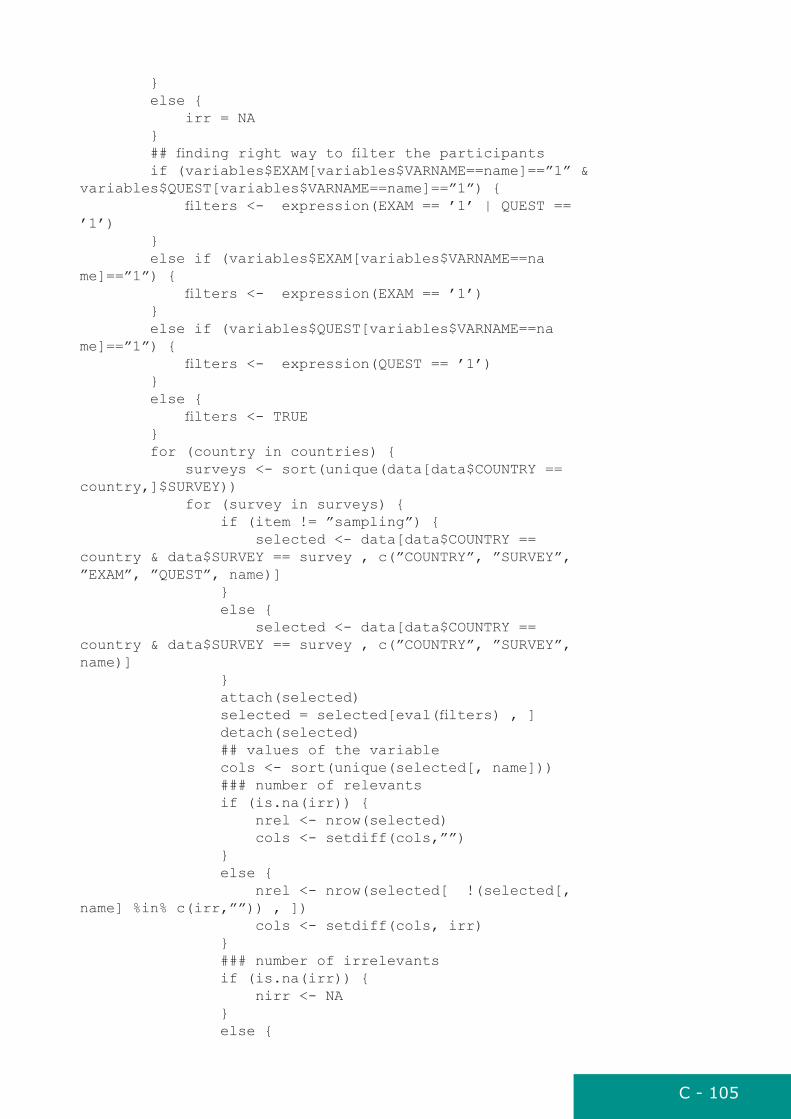
C - 105

} else { irr = NA } ## finding right way to filter the participants if (variables$EXAM[variables$VARNAME==name]==”1” & variables$QUEST[variables$VARNAME==name]==”1”) { filters <- expression(EXAM == ’1’ | QUEST == ’1’) } else if (variables$EXAM[variables$VARNAME==name]==”1”) { filters <- expression(EXAM == ’1’) } else if (variables$QUEST[variables$VARNAME==name]==”1”) { filters <- expression(QUEST == ’1’) } else { filters <- TRUE } for (country in countries) { surveys <- sort(unique(data[data$COUNTRY == country,]$SURVEY)) for (survey in surveys) { if (item != ”sampling”) { selected <- data[data$COUNTRY == country & data$SURVEY == survey , c(”COUNTRY”, ”SURVEY”, ”EXAM”, ”QUEST”, name)] } else { selected <- data[data$COUNTRY == country & data$SURVEY == survey , c(”COUNTRY”, ”SURVEY”, name)] } attach(selected) selected = selected[eval(filters) , ] detach(selected) ## values of the variable cols <- sort(unique(selected[, name])) ### number of relevants if (is.na(irr)) { nrel <- nrow(selected) cols <- setdiff(cols,””) } else { nrel <- nrow(selected[ !(selected[, name] %in% c(irr,””)) , ]) cols <- setdiff(cols, irr) } ### number of irrelevants if (is.na(irr)) { nirr <- NA } else {

C - 106

nirr <- nrow(selected[ selected[, name] %in% irr , ]) } if (is.null(tab)) { tab <- as.data.frame(cbind(country, survey, ”n_relevant”), stringsAsFactors = F ) tab[,dim(tab)[2]+1] <- nrel names(tab) <- c(”COUNTRY”, ”SURVEY”, ”FIELD”, name) } else { if ( nrow(tab[tab$COUNTRY==country & tab$SURVEY==survey & tab$FIELD==”n_relevant”,]) != 0 ) { tab[tab$COUNTRY==country & tab$SURVEY==survey & tab$FIELD==”n_relevant”, name] <- nrel } else { tab[dim(tab)[1]+1 , c(”COUNTRY”, ”SURVEY”, ”FIELD”)] <- c(country, survey, ”n_relevant”) tab[tab$COUNTRY==country & tab$SURVEY==survey & tab$FIELD==”n_relevant”, name] <- nrel } } if ( nrow(tab[tab$COUNTRY==country & tab$SURVEY==survey & tab$FIELD==”n_irrelevant”,]) != 0 ) { tab[tab$COUNTRY==country & tab$SURVEY==survey & tab$FIELD==”n_irrelevant”, name] <- nirr } else { tab[dim(tab)[1]+1 , c(”COUNTRY”, ”SURVEY”, ”FIELD”)] <- c(country, survey, ”n_irrelevant”) tab[tab$COUNTRY==country & tab$SURVEY==survey & tab$FIELD==”n_irrelevant”, name] <- nirr } if ( length(cols) != 0 ) {

for ( col in cols ) { n_field <- nrow(selected[selected[, name] == col ,]) if ( nrow(tab[tab$COUNTRY == country & tab$SURVEY== survey & tab$FIELD== col, ]) == 0 ) { tab[dim(tab)[1]+1 , c(”COUNTRY”, ”SURVEY”, ”FIELD”)] <- c(country, survey, col) tab[tab$COUNTRY==country & tab$SURVEY==survey & tab$FIELD==col, name] <- n_field } else { tab[tab$COUNTRY==country & tab$SURVEY==survey & tab$FIELD==col, name] <- n_field } n_field = NULL }

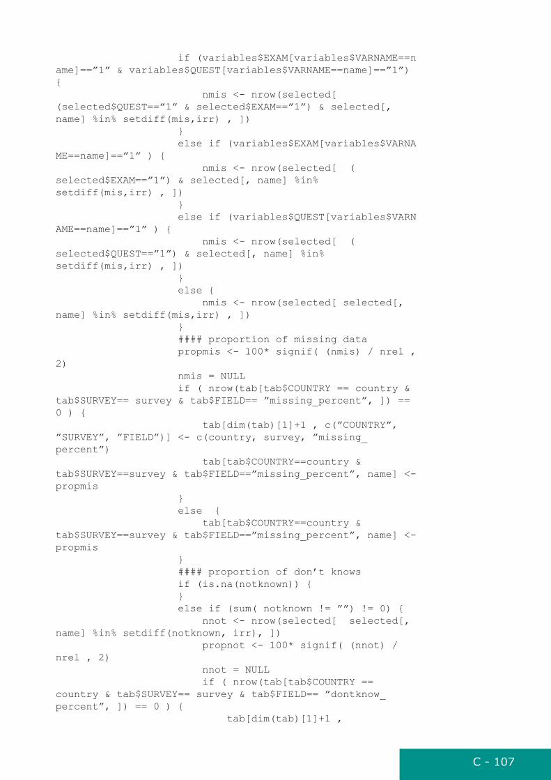
C - 107

if (variables$EXAM[variables$VARNAME==name]==”1” & variables$QUEST[variables$VARNAME==name]==”1”) { nmis <- nrow(selected[ (selected$QUEST==”1” & selected$EXAM==”1”) & selected[, name] %in% setdiff(mis,irr) , ]) } else if (variables$EXAM[variables$VARNAME==name]==”1” ) { nmis <- nrow(selected[ ( selected$EXAM==”1”) & selected[, name] %in% setdiff(mis,irr) , ]) } else if (variables$QUEST[variables$VARNAME==name]==”1” ) { nmis <- nrow(selected[ ( selected$QUEST==”1”) & selected[, name] %in% setdiff(mis,irr) , ]) } else { nmis <- nrow(selected[ selected[, name] %in% setdiff(mis,irr) , ]) } #### proportion of missing data propmis <- 100* signif( (nmis) / nrel , 2) nmis = NULL if ( nrow(tab[tab$COUNTRY == country & tab$SURVEY== survey & tab$FIELD== ”missing_percent”, ]) == 0 ) { tab[dim(tab)[1]+1 , c(”COUNTRY”, ”SURVEY”, ”FIELD”)] <- c(country, survey, ”missing_percent”) tab[tab$COUNTRY==country & tab$SURVEY==survey & tab$FIELD==”missing_percent”, name] <- propmis } else { tab[tab$COUNTRY==country & tab$SURVEY==survey & tab$FIELD==”missing_percent”, name] <- propmis } #### proportion of don’t knows if (is.na(notknown)) { } else if (sum( notknown != ””) != 0) { nnot <- nrow(selected[ selected[, name] %in% setdiff(notknown, irr), ]) propnot <- 100* signif( (nnot) / nrel , 2) nnot = NULL if ( nrow(tab[tab$COUNTRY == country & tab$SURVEY== survey & tab$FIELD== ”dontknow_percent”, ]) == 0 ) { tab[dim(tab)[1]+1 ,

C - 108

c(”COUNTRY”, ”SURVEY”, ”FIELD”)] <- c(country, survey, ”dontknow_percent”) tab[tab$COUNTRY==country & tab$SURVEY==survey & tab$FIELD==”dontknow_percent”, name] <- propnot } else { tab[tab$COUNTRY==country & tab$SURVEY==survey & tab$FIELD==”dontknow_percent”, name] <- propnot } } } } } } return(tab)}

drawtable_cont - to derive basic statistics and distribution ta-bles for continuous variables (mean, standard deviation, per-centiles, minimum and maximum values, proportion of missing values and terminal digits)

### Fuction to create dataset including distributions of continuous measurement variables, QA_DIST_XXXdrawtable_cont <- function(data, variables, item=NA, plots=F, distr=F, restr=””) { ### data = dataset, variables = definition table of variables, item = evaluation categor, plots = true if histogram is plotted tab <- NULL ## to get continuous variables varnames_cont <- sort(variables$VARNAME[variables$CONTINUOUS == 1]) if (item==”bp”) { data$BP_ROOMTEMP = gsub(” ”, ”.”, data$BP_ROOMTEMP) } if (item==”lab”) { varnames_cont = setdiff(varnames_cont, c(”BS_CHOL”, ”BS_HDL”, ”BS_GLC”, ”BS_HBA1C”)) } if (item==”smoking”) { varnames_cont <- setdiff(varnames_cont, c(”SMOKE_YEARS”, ”NUM_CIGSM”, ”NUM_CIGSH”, ”NUM_CIGARS”, ”NUM_PIPE”, ”NUM_OTHER”)) } if (item==”sampling”) { data <- data[, c(”COUNTRY”, ”SURVEY”, varnames_cont)] } else { data <- data[, c(”COUNTRY”, ”SURVEY”, ”EXAM”, ”QUEST”, varnames_cont)] }

C - 109

countries <- sort(unique(data$COUNTRY)) for (name in varnames_cont) { if (variables$IRRELEVANT[variables$VARNAME==name] != ””) { irr = variables$IRRELEVANT[variables$VARNAME==name] } else if (name %in% c(’EMPLOYMENT’, ’MEDICINE_HBP’, ’MEDICINE_DIAB’, ’MEDICINE_CHOL’, ’SMOKE_CIGSM’, ’SMOKE_CIGSH’, ’SMOKE_CIGARS’, ’SMOKE_PIPE’, ’SMOKE_OTHER’, ’NUM_CIGSM’, ’NUM_CIGSH’, ’NUM_CIGARS’, ’NUM_PIPE’, ’NUM_OTHER’, ’SMOKE_YEARS’, ’SMOKE_EVER’)) { irr = variables$IRRELEVANT[variables$VARNAME==name] } else { irr = NA } mis = variables$MISSING[variables$VARNAME==name] notknown = setdiff(variables$DONTKNOW[variables$VARNAME==name], irr) ## finding right way to filter the participants if (variables$EXAM[variables$VARNAME==name]==”1” & variables$QUEST[variables$VARNAME==name]==”1”) { filters <- expression(EXAM == ’1’ | QUEST == ’1’) } else if (variables$EXAM[variables$VARNAME==name]==”1”) { filters <- expression(EXAM == ’1’) } else if (variables$QUEST[variables$VARNAME==name]==”1”) { filters <- expression(QUEST == ’1’) } else { filters <- TRUE } for (country in countries) { surveys <- sort(unique(data[data$COUNTRY == country,]$SURVEY)) for (survey in surveys) { if (item == ”sampling”) { selected <- data[data$COUNTRY == country & data$SURVEY == survey , c(”COUNTRY”, ”SURVEY”, name)] } else { selected <- data[data$COUNTRY == country & data$SURVEY == survey , c(”COUNTRY”, ”SURVEY”, ”QUEST”, ”EXAM”, name)] } attach(selected) selected = selected[eval(filters) , ] detach(selected)

C - 110

### number of relevants if (is.na(irr)) { nrel <- nrow(selected) } else { nrel <- nrow(selected[ !(selected[, name] %in% irr) , ]) } ### number of irrelevants if (is.na(irr)) { nirr <- NA } else { nirr <- nrow(selected[ selected[, name] %in% irr , ]) } ### putting to the table if (is.null(tab)) { tab <- as.data.frame(cbind(country, survey, ”n_relevant”), stringsAsFactors = F ) tab[,dim(tab)[2]+1] <- nrel names(tab) <- c(”COUNTRY”, ”SURVEY”, ”FIELD”, name) } else { if ( nrow(tab[tab$COUNTRY==country & tab$SURVEY==survey & tab$FIELD==”n_relevant”,]) != 0 ) { tab[tab$COUNTRY==country & tab$SURVEY==survey & tab$FIELD==”n_relevant”, name] <- nrel } else { tab[dim(tab)[1]+1 , c(”COUNTRY”, ”SURVEY”, ”FIELD”)] <- c(country, survey, ”n_relevant”) tab[tab$COUNTRY==country & tab$SURVEY==survey & tab$FIELD==”n_relevant”, name] <- nrel } } if ( nrow(tab[tab$COUNTRY == country & tab$SURVEY== survey & tab$FIELD== ”n_irrelevant”, ]) == 0 ) { tab[dim(tab)[1]+1 , c(”COUNTRY”, ”SURVEY”, ”FIELD”)] <- c(country, survey, ”n_irrelevant”) tab[tab$COUNTRY==country & tab$SURVEY==survey & tab$FIELD==”n_irrelevant”, name] <- nirr } else { tab[tab$COUNTRY==country & tab$SURVEY==survey & tab$FIELD==”n_irrelevant”, name] <- nirr } if (nrel != 0) { ### Number of missing values if (variables$EXAM[variables$VARNAME==name]==”1” & variables$QUEST[variables$VARNAME==name]==”1”)

C - 111

{ nmis <- nrow(selected[ (selected$QUEST==”1” & selected$EXAM==”1”) & selected[, name] %in% mis , ]) } else if (variables$EXAM[variables$VARNAME==name]==”1” ) { nmis <- nrow(selected[ ( selected$EXAM==”1”) & selected[, name] %in% mis , ]) } else if (variables$QUEST[variables$VARNAME==name]==”1” ) { nmis <- nrow(selected[ ( selected$QUEST==”1”) & selected[, name] %in% mis , ]) } else { nmis <- nrow(selected[ selected[, name] %in% mis , ]) } ### Number of nonmissing values if (variables$EXAM[variables$VARNAME==name]==”1” & variables$QUEST[variables$VARNAME==name]==”1”) { nnonmis <- nrow(selected[ (selected$QUEST==”1” & selected$EXAM==”1”) & !(selected[, name] %in% mis) & !(selected[, name] %in% irr) & !(selected[, name] %in% notknown), ]) } else if (variables$EXAM[variables$VARNAME==name]==”1” ) { nnonmis <- nrow(selected[ ( selected$EXAM==”1”) & !(selected[, name] %in% mis) & !(selected[, name] %in% irr) & !(selected[, name] %in% notknown) , ]) } else if (variables$QUEST[variables$VARNAME==name]==”1” ) { nnonmis <- nrow(selected[ ( selected$QUEST==”1”) & !(selected[, name] %in% mis) & !(selected[, name] %in% irr) & !(selected[, name] %in% notknown), ]) } else { nnonmis <- nrow(selected[ !(selected[, name] %in% mis) & !(selected[, name] %in% irr) & !(selected[, name] %in% notknown) , ]) } ### putting to the table if ( nrow(tab[tab$COUNTRY == country & tab$SURVEY== survey & tab$FIELD== ”n_nonmissing”, ]) == 0 ) { tab[dim(tab)[1]+1 , c(”COUNTRY”, ”SURVEY”, ”FIELD”)] <- c(country, survey, ”n_nonmissing”) tab[tab$COUNTRY==country & tab$SURVEY==survey & tab$FIELD==”n_nonmissing”, name] <-

C - 112

nnonmis } else { tab[tab$COUNTRY==country & tab$SURVEY==survey & tab$FIELD==”n_nonmissing”, name] <- nnonmis } if ( nrow(tab[tab$COUNTRY == country & tab$SURVEY== survey & tab$FIELD== ”n_missing”, ]) == 0 ) { tab[dim(tab)[1]+1 , c(”COUNTRY”, ”SURVEY”, ”FIELD”)] <- c(country, survey, ”n_missing”) tab[tab$COUNTRY==country & tab$SURVEY==survey & tab$FIELD==”n_missing”, name] <- nmis } else { tab[tab$COUNTRY==country & tab$SURVEY==survey & tab$FIELD==”n_missing”, name] <- nmis } ### proportion of missing data propmis <- 100* signif( (nmis) / nrel , 2) nnonmis = NULL nmis = NULL nirr = NULL ## putting to the table if ( nrow(tab[tab$COUNTRY == country & tab$SURVEY== survey & tab$FIELD== ”missing_percent”, ]) == 0 ) { tab[dim(tab)[1]+1 , c(”COUNTRY”, ”SURVEY”, ”FIELD”)] <- c(country, survey, ”missing_percent”) tab[tab$COUNTRY==country & tab$SURVEY==survey & tab$FIELD==”missing_percent”, name] <- propmis } else { tab[tab$COUNTRY==country & tab$SURVEY==survey & tab$FIELD==”missing_percent”, name] <- propmis } #### proportion of dont knows if (is.na(notknown)) { } else if (sum( notknown != ””) != 0) { nnot <- nrow(selected[ selected[, name] %in% notknown, ]) propnot <- 100* signif( (nnot) / nrel , 2) nnot = NULL if ( nrow(tab[tab$COUNTRY == country & tab$SURVEY== survey & tab$FIELD== ”dontknow_percent”, ]) == 0 ) { tab[dim(tab)[1]+1 , c(”COUNTRY”, ”SURVEY”, ”FIELD”)] <- c(country, survey, ”dontknow_percent”)

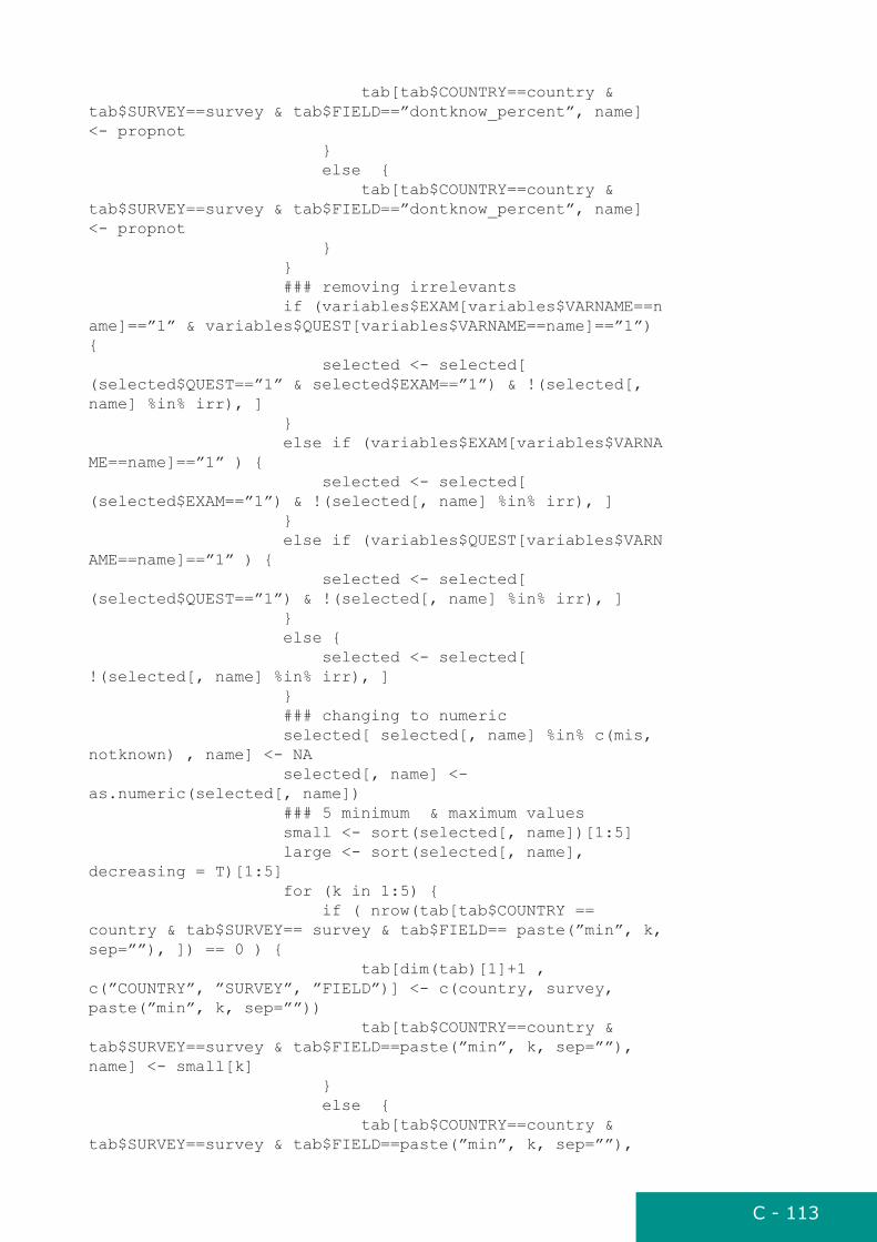
C - 113

tab[tab$COUNTRY==country & tab$SURVEY==survey & tab$FIELD==”dontknow_percent”, name] <- propnot } else { tab[tab$COUNTRY==country & tab$SURVEY==survey & tab$FIELD==”dontknow_percent”, name] <- propnot } } ### removing irrelevants if (variables$EXAM[variables$VARNAME==name]==”1” & variables$QUEST[variables$VARNAME==name]==”1”) { selected <- selected[ (selected$QUEST==”1” & selected$EXAM==”1”) & !(selected[, name] %in% irr), ] } else if (variables$EXAM[variables$VARNAME==name]==”1” ) { selected <- selected[ (selected$EXAM==”1”) & !(selected[, name] %in% irr), ] } else if (variables$QUEST[variables$VARNAME==name]==”1” ) { selected <- selected[ (selected$QUEST==”1”) & !(selected[, name] %in% irr), ] } else { selected <- selected[ !(selected[, name] %in% irr), ] } ### changing to numeric selected[ selected[, name] %in% c(mis, notknown) , name] <- NA selected[, name] <- as.numeric(selected[, name]) ### 5 minimum & maximum values small <- sort(selected[, name])[1:5] large <- sort(selected[, name], decreasing = T)[1:5] for (k in 1:5) { if ( nrow(tab[tab$COUNTRY == country & tab$SURVEY== survey & tab$FIELD== paste(”min”, k, sep=””), ]) == 0 ) { tab[dim(tab)[1]+1 , c(”COUNTRY”, ”SURVEY”, ”FIELD”)] <- c(country, survey, paste(”min”, k, sep=””)) tab[tab$COUNTRY==country & tab$SURVEY==survey & tab$FIELD==paste(”min”, k, sep=””), name] <- small[k] } else { tab[tab$COUNTRY==country & tab$SURVEY==survey & tab$FIELD==paste(”min”, k, sep=””),

C - 114

name] <- small[k] } if ( nrow(tab[tab$COUNTRY == country & tab$SURVEY== survey & tab$FIELD== paste(”max”, k, sep=””), ]) == 0 ) { tab[dim(tab)[1]+1 , c(”COUNTRY”, ”SURVEY”, ”FIELD”)] <- c(country, survey, paste(”max”, k, sep=””)) tab[tab$COUNTRY==country & tab$SURVEY==survey & tab$FIELD==paste(”max”, k, sep=””), name] <- large[k] } else { tab[tab$COUNTRY==country & tab$SURVEY==survey & tab$FIELD==paste(”max”, k, sep=””), name] <- large[k] } } small <- NULL large = NULL ### percentiles quantiles <- quantile(selected[, name], probs = c(0.1, 0.5, 0.9), na.rm=T) p <- c(10, 50, 90) for (k in 1:3) { if ( nrow(tab[tab$COUNTRY == country & tab$SURVEY== survey & tab$FIELD== paste(”percentile”, p[k], sep=””), ]) == 0 ) { tab[dim(tab)[1]+1 , c(”COUNTRY”, ”SURVEY”, ”FIELD”)] <- c(country, survey, paste(”percentile”, p[k], sep=””)) tab[tab$COUNTRY==country & tab$SURVEY==survey & tab$FIELD==paste(”percentile”, p[k], sep=””), name] <- quantiles[k] } else { tab[tab$COUNTRY==country & tab$SURVEY==survey & tab$FIELD==paste(”percentile”, p[k], sep=””), name] <- quantiles[k] } } quantiles <- NULL

## mean and SD m <- mean(selected[, name], na.rm=T) std <- sd(selected[, name], na.rm=T) if ( nrow(tab[tab$COUNTRY == country & tab$SURVEY== survey & tab$FIELD== ”mean”, ]) == 0 ) { tab[dim(tab)[1]+1 , c(”COUNTRY”, ”SURVEY”, ”FIELD”)] <- c(country, survey, ”mean”) tab[tab$COUNTRY==country & tab$SURVEY==survey & tab$FIELD==”mean”, name] <- m } else { tab[tab$COUNTRY==country &

C - 115

tab$SURVEY==survey & tab$FIELD==”mean”, name] <- m } if ( nrow(tab[tab$COUNTRY == country & tab$SURVEY== survey & tab$FIELD== ”std”, ]) == 0 ) { tab[dim(tab)[1]+1 , c(”COUNTRY”, ”SURVEY”, ”FIELD”)] <- c(country, survey, ”std”) tab[tab$COUNTRY==country & tab$SURVEY==survey & tab$FIELD==”std”, name] <- std } else { tab[tab$COUNTRY==country & tab$SURVEY==survey & tab$FIELD==”std”, name] <- std } m=NULL std=NULL

# proportion of odd readings if (grepl(”BP_”, name, ignore.case = T)) { selected$odd[ as.numeric(selected[, name]) %% 2 != 0] <- 1 odd <- 100* round((sum(selected$odd, na.rm=T) / nrel), 3) if ( nrow(tab[tab$COUNTRY == country & tab$SURVEY== survey & tab$FIELD== ”odd_percent”, ]) == 0 ) { tab[dim(tab)[1]+1 , c(”COUNTRY”, ”SURVEY”, ”FIELD”)] <- c(country, survey, ”odd_percent”) tab[tab$COUNTRY==country & tab$SURVEY==survey & tab$FIELD==”odd_percent”, name] <- odd } else { tab[tab$COUNTRY==country & tab$SURVEY==survey & tab$FIELD==”odd_percent”, name] <- odd } odd = NULL }

if (item != ”sampling”) { ## terminal digits, last digit if (name %in% c(”HEIGHT”, ”WAIST”)) { selected[, name] = format(round(selected[, name],1), nsmall=1, trim=T) } else if (name == ”WEIGHT”) { selected[, name] = format(round(selected[, name],2), nsmall=2, trim=T) } else { selected[, name] = format(selected[, name] ) } l0 <- 100* (round( sum(

C - 116

substr(selected[, name], nchar(selected[, name]) , nchar(selected[, name])) == ”0” ,na.rm=T) / sum(selected[, name] != ”NA”) , 3)) l1 <- 100* (round( sum( substr(selected[, name], nchar(selected[, name]) , nchar(selected[, name])) == ”1” ,na.rm=T) / sum(selected[, name] != ”NA”) , 3)) l2 <- 100* (round( sum( substr(selected[, name], nchar(selected[, name]) , nchar(selected[, name])) == ”2” ,na.rm=T) / sum(selected[, name] != ”NA”) , 3)) l3 <- 100* (round( sum( substr(selected[, name], nchar(selected[, name]) , nchar(selected[, name])) == ”3” ,na.rm=T) / sum(selected[, name] != ”NA”) , 3)) l4 <- 100* (round( sum( substr(selected[, name], nchar(selected[, name]) , nchar(selected[, name])) == ”4” ,na.rm=T) / sum(selected[, name] != ”NA”) , 3)) l5 <- 100* (round( sum( substr(selected[, name], nchar(selected[, name]) , nchar(selected[, name])) == ”5” ,na.rm=T) / sum(selected[, name] != ”NA”) , 3)) l6 <- 100* (round( sum( substr(selected[, name], nchar(selected[, name]) , nchar(selected[, name])) == ”6” ,na.rm=T) / sum(selected[, name] != ”NA”) , 3)) l7 <- 100* (round( sum( substr(selected[, name], nchar(selected[, name]) , nchar(selected[, name])) == ”7” ,na.rm=T) / sum(selected[, name] != ”NA”) , 3)) l8 <- 100* (round( sum( substr(selected[, name], nchar(selected[, name]) , nchar(selected[, name])) == ”8” ,na.rm=T) / sum(selected[, name] != ”NA”) , 3)) l9 <- 100* (round( sum( substr(selected[, name], nchar(selected[, name]) , nchar(selected[, name])) == ”9” ,na.rm=T) / sum(selected[, name] != ”NA”) , 3)) if ( nrow(tab[tab$COUNTRY == country & tab$SURVEY== survey & tab$FIELD== ”terminaldigit_0”, ]) == 0 ) { tab[dim(tab)[1]+1 , c(”COUNTRY”, ”SURVEY”, ”FIELD”)] <- c(country, survey, ”terminaldigit_0”) tab[tab$COUNTRY==country & tab$SURVEY==survey & tab$FIELD==”terminaldigit_0”, name] <- l0 tab[dim(tab)[1]+1 , c(”COUNTRY”, ”SURVEY”, ”FIELD”)] <- c(country, survey, ”terminaldigit_1”) tab[tab$COUNTRY==country & tab$SURVEY==survey & tab$FIELD==”terminaldigit_1”, name] <- l1 tab[dim(tab)[1]+1 ,

C - 117

c(”COUNTRY”, ”SURVEY”, ”FIELD”)] <- c(country, survey, ”terminaldigit_2”) tab[tab$COUNTRY==country & tab$SURVEY==survey & tab$FIELD==”terminaldigit_2”, name] <- l2 tab[dim(tab)[1]+1 , c(”COUNTRY”, ”SURVEY”, ”FIELD”)] <- c(country, survey, ”terminaldigit_3”) tab[tab$COUNTRY==country & tab$SURVEY==survey & tab$FIELD==”terminaldigit_3”, name] <- l3 tab[dim(tab)[1]+1 , c(”COUNTRY”, ”SURVEY”, ”FIELD”)] <- c(country, survey, ”terminaldigit_4”) tab[tab$COUNTRY==country & tab$SURVEY==survey & tab$FIELD==”terminaldigit_4”, name] <- l4 tab[dim(tab)[1]+1 , c(”COUNTRY”, ”SURVEY”, ”FIELD”)] <- c(country, survey, ”terminaldigit_5”) tab[tab$COUNTRY==country & tab$SURVEY==survey & tab$FIELD==”terminaldigit_5”, name] <- l5 tab[dim(tab)[1]+1 , c(”COUNTRY”, ”SURVEY”, ”FIELD”)] <- c(country, survey, ”terminaldigit_6”) tab[tab$COUNTRY==country & tab$SURVEY==survey & tab$FIELD==”terminaldigit_6”, name] <- l6 tab[dim(tab)[1]+1 , c(”COUNTRY”, ”SURVEY”, ”FIELD”)] <- c(country, survey, ”terminaldigit_7”) tab[tab$COUNTRY==country & tab$SURVEY==survey & tab$FIELD==”terminaldigit_7”, name] <- l7 tab[dim(tab)[1]+1 , c(”COUNTRY”, ”SURVEY”, ”FIELD”)] <- c(country, survey, ”terminaldigit_8”) tab[tab$COUNTRY==country & tab$SURVEY==survey & tab$FIELD==”terminaldigit_8”, name] <- l8 tab[dim(tab)[1]+1 , c(”COUNTRY”, ”SURVEY”, ”FIELD”)] <- c(country, survey, ”terminaldigit_9”) tab[tab$COUNTRY==country & tab$SURVEY==survey & tab$FIELD==”terminaldigit_9”, name] <- l9 } else { tab[tab$COUNTRY==country & tab$SURVEY==survey & tab$FIELD==”terminaldigit_0”, name] <- l0 tab[tab$COUNTRY==country & tab$SURVEY==survey & tab$FIELD==”terminaldigit_1”, name] <- l1

C - 118

tab[tab$COUNTRY==country & tab$SURVEY==survey & tab$FIELD==”terminaldigit_2”, name] <- l2 tab[tab$COUNTRY==country & tab$SURVEY==survey & tab$FIELD==”terminaldigit_3”, name] <- l3 tab[tab$COUNTRY==country & tab$SURVEY==survey & tab$FIELD==”terminaldigit_4”, name] <- l4 tab[tab$COUNTRY==country & tab$SURVEY==survey & tab$FIELD==”terminaldigit_5”, name] <- l5 tab[tab$COUNTRY==country & tab$SURVEY==survey & tab$FIELD==”terminaldigit_6”, name] <- l6 tab[tab$COUNTRY==country & tab$SURVEY==survey & tab$FIELD==”terminaldigit_7”, name] <- l7 tab[tab$COUNTRY==country & tab$SURVEY==survey & tab$FIELD==”terminaldigit_8”, name] <- l8 tab[tab$COUNTRY==country & tab$SURVEY==survey & tab$FIELD==”terminaldigit_9”, name] <- l9 } ## terminal digits, second last digit if (name %in% c(”HEIGHT”, ”WAIST”)) { l20 <- 100* (round( sum( substr(selected[, name], nchar(selected[, name])-2 , nchar(selected[, name])-2) == ”0” ,na.rm=T) / sum(selected[, name] != ”NA”) , 3)) l21 <- 100* (round( sum( substr(selected[, name], nchar(selected[, name])-2 , nchar(selected[, name])-2) == ”1” ,na.rm=T) / sum(selected[, name] != ”NA”) , 3)) l22 <- 100* (round( sum( substr(selected[, name], nchar(selected[, name])-2 , nchar(selected[, name])-2) == ”2” ,na.rm=T) / sum(selected[, name] != ”NA”) , 3)) l23 <- 100* (round( sum( substr(selected[, name], nchar(selected[, name])-2 , nchar(selected[, name])-2) == ”3” ,na.rm=T) / sum(selected[, name] != ”NA”) , 3)) l24 <- 100* (round( sum( substr(selected[, name], nchar(selected[, name])-2 , nchar(selected[, name])-2) == ”4” ,na.rm=T) / sum(selected[, name] != ”NA”) , 3)) l25 <- 100* (round( sum( substr(selected[, name], nchar(selected[, name])-2 , nchar(selected[, name])-2) == ”5” ,na.rm=T) / sum(selected[, name] != ”NA”) , 3)) l26 <- 100* (round( sum( substr(selected[, name], nchar(selected[, name])-

C - 119

2 , nchar(selected[, name])-2) == ”6” ,na.rm=T) / sum(selected[, name] != ”NA”) , 3)) l27 <- 100* (round( sum( substr(selected[, name], nchar(selected[, name])-2 , nchar(selected[, name])-2) == ”7” ,na.rm=T) / sum(selected[, name] != ”NA”) , 3)) l28 <- 100* (round( sum( substr(selected[, name], nchar(selected[, name])-2 , nchar(selected[, name])-2) == ”8” ,na.rm=T) / sum(selected[, name] != ”NA”) , 3)) l29 <- 100* (round( sum( substr(selected[, name], nchar(selected[, name])-2 , nchar(selected[, name])-2) == ”9” ,na.rm=T) / sum(selected[, name] != ”NA”) , 3)) } else { l20 <- 100* (round( sum( substr(selected[, name], nchar(selected[, name])-1 , nchar(selected[, name])-1) == ”0” ,na.rm=T) / sum(selected[, name] != ”NA”) , 3)) l21 <- 100* (round( sum( substr(selected[, name], nchar(selected[, name])-1 , nchar(selected[, name])-1) == ”1” ,na.rm=T) / sum(selected[, name] != ”NA”) , 3)) l22 <- 100* (round( sum( substr(selected[, name], nchar(selected[, name])-1 , nchar(selected[, name])-1) == ”2” ,na.rm=T) / sum(selected[, name] != ”NA”) , 3)) l23 <- 100* (round( sum( substr(selected[, name], nchar(selected[, name])-1 , nchar(selected[, name])-1) == ”3” ,na.rm=T) / sum(selected[, name] != ”NA”) , 3)) l24 <- 100* (round( sum( substr(selected[, name], nchar(selected[, name])-1 , nchar(selected[, name])-1) == ”4” ,na.rm=T) / sum(selected[, name] != ”NA”) , 3)) l25 <- 100* (round( sum( substr(selected[, name], nchar(selected[, name])-1 , nchar(selected[, name])-1) == ”5” ,na.rm=T) / sum(selected[, name] != ”NA”) , 3)) l26 <- 100* (round( sum( substr(selected[, name], nchar(selected[, name])-1 , nchar(selected[, name])-1) == ”6” ,na.rm=T) / sum(selected[, name] != ”NA”) , 3)) l27 <- 100* (round( sum( substr(selected[, name], nchar(selected[, name])-1 , nchar(selected[, name])-1) == ”7” ,na.rm=T) / sum(selected[, name] != ”NA”) , 3)) l28 <- 100* (round( sum( substr(selected[, name], nchar(selected[, name])-1 , nchar(selected[, name])-1) == ”8” ,na.rm=T) / sum(selected[, name] != ”NA”) , 3)) l29 <- 100* (round( sum( substr(selected[, name], nchar(selected[, name])-1 , nchar(selected[, name])-1) == ”9” ,na.rm=T) /

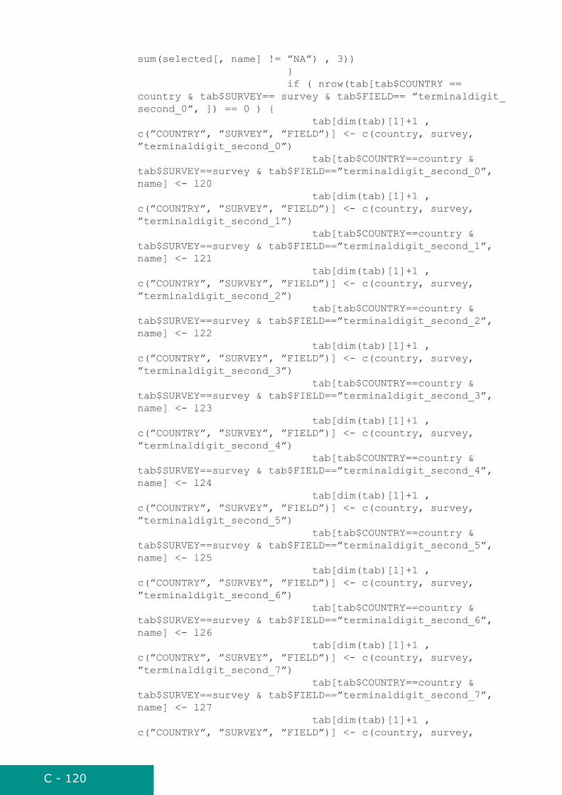
C - 120

sum(selected[, name] != ”NA”) , 3)) } if ( nrow(tab[tab$COUNTRY == country & tab$SURVEY== survey & tab$FIELD== ”terminaldigit_second_0”, ]) == 0 ) { tab[dim(tab)[1]+1 , c(”COUNTRY”, ”SURVEY”, ”FIELD”)] <- c(country, survey, ”terminaldigit_second_0”) tab[tab$COUNTRY==country & tab$SURVEY==survey & tab$FIELD==”terminaldigit_second_0”, name] <- l20 tab[dim(tab)[1]+1 , c(”COUNTRY”, ”SURVEY”, ”FIELD”)] <- c(country, survey, ”terminaldigit_second_1”) tab[tab$COUNTRY==country & tab$SURVEY==survey & tab$FIELD==”terminaldigit_second_1”, name] <- l21 tab[dim(tab)[1]+1 , c(”COUNTRY”, ”SURVEY”, ”FIELD”)] <- c(country, survey, ”terminaldigit_second_2”) tab[tab$COUNTRY==country & tab$SURVEY==survey & tab$FIELD==”terminaldigit_second_2”, name] <- l22 tab[dim(tab)[1]+1 , c(”COUNTRY”, ”SURVEY”, ”FIELD”)] <- c(country, survey, ”terminaldigit_second_3”) tab[tab$COUNTRY==country & tab$SURVEY==survey & tab$FIELD==”terminaldigit_second_3”, name] <- l23 tab[dim(tab)[1]+1 , c(”COUNTRY”, ”SURVEY”, ”FIELD”)] <- c(country, survey, ”terminaldigit_second_4”) tab[tab$COUNTRY==country & tab$SURVEY==survey & tab$FIELD==”terminaldigit_second_4”, name] <- l24 tab[dim(tab)[1]+1 , c(”COUNTRY”, ”SURVEY”, ”FIELD”)] <- c(country, survey, ”terminaldigit_second_5”) tab[tab$COUNTRY==country & tab$SURVEY==survey & tab$FIELD==”terminaldigit_second_5”, name] <- l25 tab[dim(tab)[1]+1 , c(”COUNTRY”, ”SURVEY”, ”FIELD”)] <- c(country, survey, ”terminaldigit_second_6”) tab[tab$COUNTRY==country & tab$SURVEY==survey & tab$FIELD==”terminaldigit_second_6”, name] <- l26 tab[dim(tab)[1]+1 , c(”COUNTRY”, ”SURVEY”, ”FIELD”)] <- c(country, survey, ”terminaldigit_second_7”) tab[tab$COUNTRY==country & tab$SURVEY==survey & tab$FIELD==”terminaldigit_second_7”, name] <- l27 tab[dim(tab)[1]+1 , c(”COUNTRY”, ”SURVEY”, ”FIELD”)] <- c(country, survey,

C - 121

”terminaldigit_second_8”) tab[tab$COUNTRY==country & tab$SURVEY==survey & tab$FIELD==”terminaldigit_second_8”, name] <- l28 tab[dim(tab)[1]+1 , c(”COUNTRY”, ”SURVEY”, ”FIELD”)] <- c(country, survey, ”terminaldigit_second_9”) tab[tab$COUNTRY==country & tab$SURVEY==survey & tab$FIELD==”terminaldigit_second_9”, name] <- l29 } else { tab[tab$COUNTRY==country & tab$SURVEY==survey & tab$FIELD==”terminaldigit_second_0”, name] <- l20 tab[tab$COUNTRY==country & tab$SURVEY==survey & tab$FIELD==”terminaldigit_second_1”, name] <- l21 tab[tab$COUNTRY==country & tab$SURVEY==survey & tab$FIELD==”terminaldigit_second_2”, name] <- l22 tab[tab$COUNTRY==country & tab$SURVEY==survey & tab$FIELD==”terminaldigit_second_3”, name] <- l23 tab[tab$COUNTRY==country & tab$SURVEY==survey & tab$FIELD==”terminaldigit_second_4”, name] <- l24 tab[tab$COUNTRY==country & tab$SURVEY==survey & tab$FIELD==”terminaldigit_second_5”, name] <- l25 tab[tab$COUNTRY==country & tab$SURVEY==survey & tab$FIELD==”terminaldigit_second_6”, name] <- l26 tab[tab$COUNTRY==country & tab$SURVEY==survey & tab$FIELD==”terminaldigit_second_7”, name] <- l27 tab[tab$COUNTRY==country & tab$SURVEY==survey & tab$FIELD==”terminaldigit_second_8”, name] <- l28 tab[tab$COUNTRY==country & tab$SURVEY==survey & tab$FIELD==”terminaldigit_second_9”, name] <- l29 } # proportion of even values even <- sum(c(l0,l2,l4,l6,l8),na.rm=T ) if ( nrow(tab[tab$COUNTRY == country & tab$SURVEY== survey & tab$FIELD== ”terminal_even_percent”, ]) == 0 ) { tab[dim(tab)[1]+1 , c(”COUNTRY”, ”SURVEY”, ”FIELD”)] <- c(country, survey, ”terminal_even_percent”) tab[tab$COUNTRY==country & tab$SURVEY==survey & tab$FIELD==”terminal_even_percent”, name] <- even

C - 122

} else { tab[tab$COUNTRY==country & tab$SURVEY==survey & tab$FIELD==”terminal_even_percent”, name] <- even } even = NULL even2 <- sum(c(l20,l22,l24,l26,l28),na.rm=T ) if ( nrow(tab[tab$COUNTRY == country & tab$SURVEY== survey & tab$FIELD== ”terminalsecond_even_percent”, ]) == 0 ) { tab[dim(tab)[1]+1 , c(”COUNTRY”, ”SURVEY”, ”FIELD”)] <- c(country, survey, ”terminalsecond_even_percent”) tab[tab$COUNTRY==country & tab$SURVEY==survey & tab$FIELD==”terminalsecond_even_percent”, name] <- even2 } else { tab[tab$COUNTRY==country & tab$SURVEY==survey & tab$FIELD==”terminalsecond_even_percent”, name] <- even2 } even2 = NULL } } } } } return(tab)}

plotdist - to plot simple distribution plot for continuous vari-ables (png file)

plotdist <- function(data, varname, outpath, div, minim, maxim, mis=NA, irr=NA, axmin=minim, axmax=maxim) { ### data = dataset, varname = name of the variable, outpath = path to save the file, minim = lower limit of the variable, maxim = upper limit of the variable, ### mis = code for missing value, irr = code for irrelevants, axmin = minimum of the x-axis, axmax = minimum of the x-axis return=T variable <-data[, varname] novalue <- (variable %in% mis) totallymis <- (variable %in% irr) if (sum(totallymis) + sum(novalue) == length(variable)) { return = FALSE } variable <- as.numeric(variable[!novalue & !totallymis]) if (sum(variable >= minim & variable <= maxim) == 0) {

C - 123

return = FALSE } counts <- table(variable[variable >= minim & variable <= maxim]) classes <- as.numeric(names(counts)) divpoints <- ((classes %% div) == 0) if (return) { png(file = paste(outpath, tolower(data$COUNTRY[1]), data$SURVEY[1], ’_’, tolower(varname), ’.png’, sep=’’), width=800, height=600)

plot(classes, counts, type=’h’, axes=FALSE, main=paste(varname, ’ (’, data$COUNTRY[1], ’survey’, data$SURVEY[1], ’)’), xlab=varname, ylab=’N’, xlim=c(minim, maxim), ylim=c(0, max(counts)))

points(classes, counts, cex=0.6)

# Number of outliers in the right: outl <- sum(variable > maxim) if (outl > 0) mtext(paste(outl, ’ obs.\n>’, maxim, sep=’’), side=1, line=3, at=maxim, cex=0.9) # Number of outliers in the left: outl <- sum(variable < minim) if (outl > 0) mtext(paste(outl, ’ obs.\n<’, minim, sep=’’), side=1, line=3, at=minim, cex=0.9) ## Number of observations and missing values mtext(paste(’n_relevant = ’,length(variable) + sum(novalue, na.rm=T), sep=’’), side=3, line=-2, cex=0.9, adj=1) mtext(paste(sum(novalue), ’ missing’, sep=’’), side=3, line=-3, cex=0.9, adj=1) box() axis(1, at=seq(axmin, axmax, by=div), labels=seq(axmin, axmax, by=div), cex.axis=0.9) axis(2, cex.axis=0.9) mtext(paste(’Updated on’, Sys.Date()), side=3, line=0.3, adj=1, cex=0.9) dev.off() } variable = NULL}

create_bpdiff - to calculate differences between three blood pressure measurements

### Function to create differences between BP measurementscreate_bpdiff <- function(data, variables) { ### data = dataset, variables = definition table for variables mis = variables$MISSING[variables$VARNAME==”BP_SYST1”] irr = variables$IRRELEVANT[variables$VARNAME==”BP_

C - 124

SYST1”] ### Differences between BP measurements data$SBP1_SBP2[!(data$BP_SYST1 %in% mis) & !(data$BP_SYST2 %in% mis)] <- as.numeric(data$BP_SYST1[!(data$BP_SYST1 %in% mis) & !(data$BP_SYST2 %in% mis)]) - as.numeric(data$BP_SYST2[!(data$BP_SYST1 %in% mis) & !(data$BP_SYST2 %in% mis)]) data$SBP1_SBP2[(data$BP_SYST1 %in% mis) | (data$BP_SYST2 %in% mis)] <- mis data$SBP1_SBP2[(data$BP_SYST1 %in% irr) | (data$BP_SYST2 %in% irr)] <- irr

data$SBP2_SBP3[!(data$BP_SYST2 %in% mis) & !(data$BP_SYST3 %in% mis)] <- as.numeric(data$BP_SYST2[!(data$BP_SYST2 %in% mis) & !(data$BP_SYST3 %in% mis)]) - as.numeric(data$BP_SYST3[!(data$BP_SYST2 %in% mis) & !(data$BP_SYST3 %in% mis)]) data$SBP2_SBP3[(data$BP_SYST2 %in% mis) | (data$BP_SYST3 %in% mis)] <- mis data$SBP2_SBP3[(data$BP_SYST2 %in% irr) | (data$BP_SYST3 %in% irr)] <- irr

data$SBP1_SBP3[!(data$BP_SYST1 %in% mis) & !(data$BP_SYST3 %in% mis)] <- as.numeric(data$BP_SYST1[!(data$BP_SYST1 %in% mis) & !(data$BP_SYST3 %in% mis)]) - as.numeric(data$BP_SYST3[!(data$BP_SYST1 %in% mis) & !(data$BP_SYST3 %in% mis)]) data$SBP1_SBP3[(data$BP_SYST1 %in% mis) | (data$BP_SYST3 %in% mis)] <- mis data$SBP1_SBP3[(data$BP_SYST1 %in% irr) | (data$BP_SYST3 %in% irr)] <- irr

data$DBP1_DBP2[!(data$BP_DIAST1 %in% mis) & !(data$BP_DIAST2 %in% mis)] <- as.numeric(data$BP_DIAST1[!(data$BP_DIAST1 %in% mis) & !(data$BP_DIAST2 %in% mis)]) - as.numeric(data$BP_DIAST2[!(data$BP_DIAST1 %in% mis) & !(data$BP_DIAST2 %in% mis)]) data$DBP1_DBP2[(data$BP_DIAST1 %in% mis) | (data$BP_DIAST2 %in% mis)] <- mis data$DBP1_DBP2[(data$BP_DIAST1 %in% irr) | (data$BP_DIAST2 %in% irr)] <- irr

data$DBP2_DBP3[!(data$BP_DIAST2 %in% mis) & !(data$BP_DIAST3 %in% mis)] <- as.numeric(data$BP_DIAST2[!(data$BP_DIAST2 %in% mis) & !(data$BP_DIAST3 %in% mis)]) - as.numeric(data$BP_DIAST3[!(data$BP_DIAST2 %in% mis) & !(data$BP_DIAST3 %in% mis)]) data$DBP2_DBP3[(data$BP_DIAST2 %in% mis) | (data$BP_DIAST3 %in% mis)] <- mis data$DBP2_DBP3[(data$BP_DIAST2 %in% irr) | (data$BP_DIAST3 %in% irr)] <- irr

data$DBP1_DBP3[!(data$BP_DIAST1 %in% mis) & !(data$BP_DIAST3 %in% mis)] <- as.numeric(data$BP_DIAST1[!(data$BP_DIAST1 %in% mis) & !(data$BP_DIAST3 %in% mis)]) -

C - 125

as.numeric(data$BP_DIAST3[!(data$BP_DIAST1 %in% mis) & !(data$BP_DIAST3 %in% mis)]) data$DBP1_DBP3[(data$BP_DIAST1 %in% mis) | (data$BP_DIAST3 %in% mis)] <- mis data$DBP1_DBP3[(data$BP_DIAST1 %in% irr) | (data$BP_DIAST3 %in% irr)] <- irr

data$DBP1_DBP2_DBP3 <- 0 data$DBP1_DBP2_DBP3[!(data$BP_DIAST1 %in% mis) & !(data$BP_DIAST2 %in% mis) & !(data$BP_DIAST3 %in% mis) & data$BP_DIAST1 == data$BP_DIAST2 & data$BP_DIAST1 == data$BP_DIAST3] <- 1 data$DBP1_DBP2_DBP3[(data$BP_DIAST1 %in% mis) | (data$BP_DIAST2 %in% mis) | (data$BP_DIAST3 %in% mis)] <- mis data$DBP1_DBP2_DBP3[(data$BP_DIAST1 %in% irr) | (data$BP_DIAST2 %in% irr) | (data$BP_DIAST3 %in% irr)] <- irr

data$SBP1_SBP2_SBP3 <- 0 data$SBP1_SBP2_SBP3[!(data$BP_SYST1 %in% mis) & !(data$BP_SYST2 %in% mis) & !(data$BP_SYST3 %in% mis) & data$BP_SYST1 == data$BP_SYST2 & data$BP_SYST1 == data$BP_SYST3] <- 1 data$SBP1_SBP2_SBP3[(data$BP_SYST1 %in% mis) | (data$BP_SYST2 %in% mis) | (data$BP_SYST3 %in% mis)] <- mis return(data)}

create_bsconv - to calculate unit conversions of lipid and glu-cose measurements

create_bsconv <- function(data, variables) { ### data = dataset, variables = definition table for variables mis = variables$MISSING[variables$VARNAME==”BS_CHOL”] irr = variables$IRRELEVANT[variables$VARNAME==”BS_CHOL”] ## Separating different units data$BS_CHOL_MMOLL[data$BS_UNIT_CHOL == ”1” ] <- data$BS_CHOL[data$BS_UNIT_CHOL == ”1” ] data$BS_CHOL_MMOLL[data$BS_UNIT_CHOL != ”1” ] <- ”.” data$BS_CHOL_MMOLL[data$BS_CHOL == mis ] <- mis data$BS_CHOL_MGDL[data$BS_UNIT_CHOL != ”2”] <-”.” data$BS_CHOL_MGDL[data$BS_UNIT_CHOL == ”2” ] <- data$BS_CHOL[data$BS_UNIT_CHOL == ”2” ] data$BS_CHOL_MGDL[data$BS_CHOL == mis ] <- mis data$BS_HDL_MMOLL[data$BS_UNIT_HDL != ”1” ] <- ”.” data$BS_HDL_MMOLL[data$BS_UNIT_HDL == ”1” ] <- data$BS_HDL[data$BS_UNIT_HDL == ”1” ] data$BS_HDL_MMOLL[data$BS_HDL == mis ] <- mis data$BS_HDL_MGDL[data$BS_UNIT_HDL != ”2”] <- ”.” data$BS_HDL_MGDL[data$BS_UNIT_HDL == ”2” ] <- data$BS_

C - 126

HDL[data$BS_UNIT_HDL == ”2” ] data$BS_HDL_MGDL[data$BS_HDL == mis ] <- mis data$BS_GLC_MMOLL[data$BS_UNIT_GLC != ”1” ] <- ”.” data$BS_GLC_MMOLL[data$BS_UNIT_GLC == ”1” ] <- data$BS_GLC[data$BS_UNIT_GLC == ”1” ] data$BS_GLC_MMOLL[data$BS_GLC == mis ] <- mis data$BS_GLC_MGDL[data$BS_UNIT_GLC != ”2”] <- ”.” data$BS_GLC_MGDL[data$BS_UNIT_GLC == ”2” ] <- data$BS_GLC[data$BS_UNIT_GLC == ”2” ] data$BS_GLC_MGDL[data$BS_GLC == mis ] <- mis data$BS_HBA1C_MMOLMOL[data$BS_UNIT_HBA1C != ”1” ] <- ”.” data$BS_HBA1C_MMOLMOL[data$BS_UNIT_HBA1C == ”1” ] <- data$BS_HBA1C[data$BS_UNIT_HBA1C == ”1” ] data$BS_HBA1C_MMOLMOL[data$BS_HBA1C == mis ] <- mis data$BS_HBA1C_PERCENT[data$BS_UNIT_HBA1C != ”2”] <- ”.” data$BS_HBA1C_PERCENT[data$BS_UNIT_HBA1C == ”2” ] <- data$BS_HBA1C[data$BS_UNIT_HBA1C == ”2” ] data$BS_HBA1C_PERCENT[data$BS_HBA1C == mis ] <- mis

return(data)}

drawtable_bpqa - to derive specific quality assessment checks for blood pressure (proportion of incomplete data, proportion of identical measurements)

drawtable_bpqa <- function(data, variables) { ### data = dataset, variables = definition table for variables # tab, output table tab <- NULL variables <- variables[grepl(”BP_SY”, variables$VARNAME, ignore.case = TRUE) | grepl(”BP_DI”, variables$VARNAME, ignore.case = TRUE),] variables[is.na(variables)] = ”” data <- data[ , c(”COUNTRY”, ”SURVEY”, ”EXAM”, variables$VARNAME)] countries <- sort(unique(data$COUNTRY)) mis = variables$MISSING[variables$VARNAME==”BP_SYST1”] irr = variables$IRRELEVANT[variables$VARNAME==”BP_SYST1”] data = create_bpdiff(data, variables) varnames = c(”SBP1_SBP2”, ”SBP2_SBP3”, ”SBP1_SBP3” ,”DBP1_DBP2” ,”DBP2_DBP3”, ”DBP1_DBP3”, ”SBP1_SBP2_SBP3”, ”DBP1_DBP2_DBP3”) for (name in varnames) { for (country in countries) { surveys <- sort(unique(data[data$COUNTRY == country,]$SURVEY)) for (survey in surveys) { selected <- data[data$COUNTRY == country & data$SURVEY == survey , c(”COUNTRY”, ”SURVEY”, ”EXAM”, name)]

C - 127

### number of non-irrelevants nrel <- nrow(selected[ ( selected$EXAM==”1”) & !(selected[, name] %in% irr) , ]) ### number of irrelevants nirr <- nrow(selected[ ( selected$EXAM==”1”) & selected[, name] %in% irr,]) ### putting to the table if (is.null(tab)) { tab <- as.data.frame(cbind(country, survey, ”n_relevant”), stringsAsFactors = F ) tab[,dim(tab)[2]+1] <- nrel names(tab) <- c(”COUNTRY”, ”SURVEY”, ”FIELD”, name) } else { if ( nrow(tab[tab$COUNTRY==country & tab$SURVEY==survey & tab$FIELD==”n_relevant”,]) != 0 ) { tab[tab$COUNTRY==country & tab$SURVEY==survey & tab$FIELD==”n_relevant”, name] <- nrel } else { tab[dim(tab)[1]+1 , c(”COUNTRY”, ”SURVEY”, ”FIELD”)] <- c(country, survey, ”n_relevant”) tab[tab$COUNTRY==country & tab$SURVEY==survey & tab$FIELD==”n_relevant”, name] <- nrel } } if ( nrow(tab[tab$COUNTRY == country & tab$SURVEY== survey & tab$FIELD== ”n_irrelevant”, ]) == 0 ) { tab[dim(tab)[1]+1 , c(”COUNTRY”, ”SURVEY”, ”FIELD”)] <- c(country, survey, ”n_irrelevant”) tab[tab$COUNTRY==country & tab$SURVEY==survey & tab$FIELD==”n_irrelevant”, name] <- nirr } else { tab[tab$COUNTRY==country & tab$SURVEY==survey & tab$FIELD==”n_irrelevant”, name] <- nirr } if (nrel != 0) { ### Number of missing values nmis <- nrow(selected[ ( selected$EXAM==”1”) & selected[, name] %in% mis , ])

### Number of nonmissing values nnonmis <- nrow(selected[ ( selected$EXAM==”1”) & !(selected[, name] %in% mis) & !(selected[, name] %in% irr) , ])

### putting to the table if ( nrow(tab[tab$COUNTRY == country & tab$SURVEY== survey & tab$FIELD== ”n_nonmissing”, ]) == 0 ) {

C - 128

tab[dim(tab)[1]+1 , c(”COUNTRY”, ”SURVEY”, ”FIELD”)] <- c(country, survey, ”n_nonmissing”) tab[tab$COUNTRY==country & tab$SURVEY==survey & tab$FIELD==”n_nonmissing”, name] <- nnonmis } else { tab[tab$COUNTRY==country & tab$SURVEY==survey & tab$FIELD==”n_nonmissing”, name] <- nnonmis } if ( nrow(tab[tab$COUNTRY == country & tab$SURVEY== survey & tab$FIELD== ”n_missing”, ]) == 0 ) { tab[dim(tab)[1]+1 , c(”COUNTRY”, ”SURVEY”, ”FIELD”)] <- c(country, survey, ”n_missing”) tab[tab$COUNTRY==country & tab$SURVEY==survey & tab$FIELD==”n_missing”, name] <- nmis } else { tab[tab$COUNTRY==country & tab$SURVEY==survey & tab$FIELD==”n_missing”, name] <- nmis } ### proportion of missing data propmis <- 100* signif( (nmis) / nrel , 2) nnonmis = NULL nmis = NULL nirr = NULL ## putting to the table if ( nrow(tab[tab$COUNTRY == country & tab$SURVEY== survey & tab$FIELD== ”missing_percent”, ]) == 0 ) { tab[dim(tab)[1]+1 , c(”COUNTRY”, ”SURVEY”, ”FIELD”)] <- c(country, survey, ”missing_percent”) tab[tab$COUNTRY==country & tab$SURVEY==survey & tab$FIELD==”missing_percent”, name] <- propmis } else { tab[tab$COUNTRY==country & tab$SURVEY==survey & tab$FIELD==”missing_percent”, name] <- propmis

} ### removing irrelevants selected <- selected[ (selected$EXAM==”1”) & !(selected[, name] %in% irr), ] if (!(name %in% c(”SBP1_SBP2_SBP3”, ”DBP1_DBP2_DBP3”))) { ### changing to numeric selected[ selected[, name] %in% mis , name] <- NA selected[, name] <- as.numeric(selected[, name])

C - 129

#proportion of identical results ident <- 100*round(nrow(selected[selected[,name] == 0, ] ) / nrel, 3) if ( nrow(tab[tab$COUNTRY == country & tab$SURVEY== survey & tab$FIELD== ”identical_percent”, ]) == 0 ) { tab[dim(tab)[1]+1 , c(”COUNTRY”, ”SURVEY”, ”FIELD”)] <- c(country, survey, ”identical_percent”) tab[tab$COUNTRY==country & tab$SURVEY==survey & tab$FIELD==”identical_percent”, name] <- ident } else { tab[tab$COUNTRY==country & tab$SURVEY==survey & tab$FIELD==”identical_percent”, name] <- ident } } else { #proportion of identical results ident <- 100*round(nrow(selected[selected[,name] == 1, ] ) / nrel, 3) if ( nrow(tab[tab$COUNTRY == country & tab$SURVEY== survey & tab$FIELD== ”identical_percent”, ]) == 0 ) { tab[dim(tab)[1]+1 , c(”COUNTRY”, ”SURVEY”, ”FIELD”)] <- c(country, survey, ”identical_percent”) tab[tab$COUNTRY==country & tab$SURVEY==survey & tab$FIELD==”identical_percent”, name] <- ident } else { tab[tab$COUNTRY==country & tab$SURVEY==survey & tab$FIELD==”identical_percent”, name] <- ident } } } } } } return(tab)}

C - 130

Part C


C - 131


The following indicators are defined to be used in EHES reporting, both in quality assessments and basic reporting of the results. For more de-tails how to calculate the indicators from EHES data see EHES Manual, Part C, Chapter 5.

Indicators which at least should be included in the basic report nation-ally and in the EHES basic report are marked with a green tick mark (v).

4.1 Definition of indicators

4.1.1 blood pressure

4.1.1.1 Systolic blood pressure (mmHg)

• Population mean, standard error and 95 % confidence in-terval v

• Population standard deviation• Order statistics: 5 minimum values, 10th percentile, 25th

percentile, 50th percentile (median), 75th percentile, 90th percentile and 5 maximum values

• Distribution curve• Cumulative distribution curve• Comment: Mean systolic blood pressure is an indicator of

WHO 2013

4.1.1.2 Diastolic blood pressure (mmHg)


• Population standard deviation• Order statistics: 5 smallest values, 10th percentile, 25th

percentile, 50th percentile (median), 75th percentile, 90th percentile and 5 largest values

4. indicatorsKari Kuulasmaa1, Päivikki Koponen1, Johanna Mäki-Opas1, Tarja Pa-losaari1, Katri Kilpeläinen1 and Hanna Tolonen1


C - 132

• Distribution curve• Cumulative distribution curve

4.1.1.3 Hypertension and categories of blood pressure

Prevalence of self-reported high blood pressure (hyper-tension) (%) v

• Definition: Proportion of those who reported that they have been diagnosed by a medical doctor to have a high blood pressure (hypertension) among all survey participants

• Comment: A subjective indicator from questionnaire data.

Prevalence of actual and potential hypertensives (%) v

• Definition: Proportion of those whose systolic blood pres-sure was at least 140 mmHg or diastolic blood pressure was at least 90 mmHg or who reported that they are taking medication to lower their blood pressure among all survey participants.

• Comment: Serves as a proxy for the prevalence of hyperten-sion in the population, whether diagnosed or undiagnosed. An objective indicator based on measured blood pressure.

Prevalence of elevated blood pressure (%)

• Definition: Proportion of those whose systolic blood pressure was at least 140 mmHg or diastolic blood pressure was at least 90 mmHg among all survey participants. (WHO 2013)

Prevalence of isolated systolic blood pressure (%)

• Definition: Proportion of those whose systolic blood pres-sure was at least 140 mmHg and diastolic blood pressure was less than 90 mmHg among all survey participants. (Pie-poli, Hoes et al. 2016)

Distribution of categories of blood pressure (%)

• Definition: Proportion of categories of blood pressure in the population (%) (Piepoli, Hoes et al. 2016)• Optimal if systolic blood pressure was less than 120

mmHg and diastolic blood pressure was less than 80 mmHg

• Normal if systolic blood pressure was 120-129 mmHg and/or diastolic blood pressure was 80-84 mmHg and neither of these is above the upper limit

C - 133

• High normal if systolic blood pressure was 130-139 mmHg and/or diastolic blood pressure was 85-89 mmHg and neither of these is above the upper limit

• Grade 1 hypertension if systolic blood pressure was 140-159 mmHg and/or diastolic blood pressure was 90-99 mmHg and neither of these is above the upper limit

• Grade 2 hypertension if systolic blood pressure was 160-179 mmHg and/or diastolic blood pressure was 100-109 mmHg and neither of these is above the upper limit

• Grade 3 hypertension if systolic blood pressure was at least 180 mmHg and/or diastolic blood pressure was at least 110 mmHg

4.1.1.4 awareness of elevated blood pressure

awareness of elevated blood pressure among actual and potential hypertensives (%) v

• Definition: Proportion of those who reported that they have been diagnosed by a medical doctor to have a high blood pressure (hypertension) among those defined as having ac-tual or potential hypertension.

4.1.1.5 anti-hypertensive drug use

Prevalence of anti-hypertensive drug use in the popula-tion (%) v

• Definition: Proportion of those who reported that they are taking medication to lower their blood pressure among all survey participants.

Prevalence of anti-hypertensive drug use among actual and potential hypertensives (%) v

• Definition: Proportion of those who reported that they are taking medication to lower their blood pressure among those defined as having actual or potential hypertension.

Prevalence of optimal blood pressure among those using anti-hypertensive drugs (%) v

• Definition: Proportion of those whose systolic blood pres-sure is below 140 mmHg and diastolic blood pressure below 90 mmHg among those who report taking medication to lower their blood pressure.

C - 134

4.1.1.6 blood pressure measurement

Proportion of the population with blood pressure measurement in the past 12 months (%)

• Definition: Proportion of those who reported that their blood pressure was measured by a health professional in the past 12 months among all survey participants.

Proportion of the population with blood pressure measurement in the past 5 years (%) v

• Definition: Proportion of those who reported that their blood pressure was measured by a health professional in the past 5 years among all survey participants.

4.1.1.7 Pulse rate (beats/min)

• Population mean, standard error and 95 % confidence in-terval

• Population standard deviation• Order statistics: 5 smallest values, 10th percentile, median,

90th percentile and 5 largest values• Distribution curve• Cumulative distribution curve

4.1.2 lipids

4.1.2.1 Serum total cholesterol (mmol/l)




• Distribution curve• Cumulative distribution curve• Comment: Mean total cholesterol concentration is an indica-

tor of WHO 2013.

4.1.2.2 Serum high-density lipoprotein (HDl) cholesterol (mmol/l)


C - 135




4.1.2.3 Serum non-HDl cholesterol (mmol/l)


• Population standard deviation • Order statistics: 5 minimum values, 10th percentile, 25th


• Distribution curve

• Cumulative distribution curve

4.1.2.4 Serum total cholesterol to HDl cholesterol ratio






4.1.2.5 Categories of cholesterol level

Prevalence of self-reported elevated blood cholesterol (%) v

• Definition: Proportion of those who reported that they have been diagnosed by a medical doctor to have elevated blood cholesterol among all survey participants.

• Comment: A subjective indicator of elevated blood choles-terol.

Prevalence of elevated serum total cholesterol in the population (%)

• Definition: Proportion of those whose serum total choles-terol was at least 5.0 mmol/l among all survey participants.

C - 136

• Comment: Serves as a proxy for the prevalence of elevated total serum cholesterol in the population.

Prevalence of actual or potential elevated serum total cholesterol in the population (%) v

• Definition: Proportion of those whose serum total choles-terol was at least 5.0 mmol/l or who reported that they are taking medication to lower their blood cholesterol among all survey participants. (WHO 2013)

Distribution of categories of serum total cholesterol (%)

• Definition: Proportion of categories of serum total choles-terol in population (%) among all survey participants• below 5.0 mmol/l• at least 5.0 mmol/l and below 6.0 mmol/l• at least 6.0 mmol/l and below 7.0 mmol/l• at least 7.0 mmol/l and below 8.0 mmol/l

• at least 8.0 mmol/l

Prevalence of low HDl cholesterol (%)

• Definition: Proportion of those whose HDL cholesterol is lower than 1.0 mmol/l in men and lower than 1.2 mmol/l in women among all survey participants. (Piepoli, Hoes et al. 2016)

Prevalence of high total cholesterol to HDl cholesterol ratio (%)

• Definition: Proportion of those who whose serum total cho-lesterol to HDL cholesterol ratio is greater than 5 among all survey participants.

Prevalence of elevated non-HDl cholesterol (%)

• Definition: Proportion of those whose non-HDL cholesterol is greater than 3.5 mmol/l among all survey participants.

Prevalence of actual or potential elevated non-HDl cho-lesterol in the population (%)

• Definition: Proportion of those whose non-HDL cholesterol is greater than 3.5 mmol/l or who reported that they are tak-ing medications to lower their blood cholesterol among all survey participants.

C - 137

4.1.2.6 awareness of elevated total cholesterol

awareness of elevated serum cholesterol among those with actual or potential elevated serum total cholesterol (%) v

• Definition: Proportion of those who reported that they have been diagnosed by a medical doctor to have elevated blood cholesterol among those defined as having actual or poten-tial elevated serum total cholesterol.

4.1.2.7 lipid lowering drug use

Prevalence of lipid lowering drug use in the population (%) v

• Definition: Proportion of those who reported that they are taking medication to lower their blood cholesterol among all survey participants.

Prevalence of lipid lowering drug use among those with elevated total cholesterol (%) v

• Definition: Proportion of those who reported that they are taking medication to lower their blood cholesterol among those defined as having elevated serum total cholesterol.

Prevalence of optimal total cholesterol level among those using lipid lowering drugs (%) v

• Definition: Proportion of those whose serum total choles-terol is less than 5.0 mmol/l among those who are taking medication to lower their blood cholesterol.

4.1.2.8 Cholesterol measurement

Proportion of the population with cholesterol measure-ment in the past 12 months (%)

• Definition: Proportion of those who reported that their blood cholesterol have been measured by a health professional in the past 12 months among all survey participants.

Proportion of the population with cholesterol measure-ment in the past 5 years (%) v

• Definition: Proportion of those who reported that their blood cholesterol have been measured by a health professional in the past 5 years among all survey participants.

C - 138

4.1.3 Glucose

4.1.3.1 Fasting plasma glucose





4.1.3.2 Glycated haemoglobin (Hba1c)




• Distribution curve• Cumulative distribution curves

4.1.3.3 Diabetes and impaired fasting glucose

Prevalence of self-reported diabetes (%) v (EHCI indicator name: Diabetes: self-reported prevalence)

• Definition: Proportion of those who reported that they have been diagnosed by a medical doctor to have diabetes among all survey participants.

• Comment: A subjective indicator.

Prevalence of impaired fasting glucose (iFG) (%)

• Definition: Proportion of those with fasting plasma glucose more than 6.0 mmol/l but less than 7.0 mmol/l (WHO 2006) among all survey participants.

Prevalence of raised blood glucose/diabetes (%) based on fasting plasma glucose

• Definition: Proportion of those with fasting plasma glucose at least 7.0 mmol/l (WHO 2006) among all survey partici-pants.

C - 139

Prevalence of raised blood glucose/diabetes (%) based on Hba1c

• Definition: Proportion of those with HbA1c at least 6.5% in the NGSP (National Glycohemoglobin Standardization Program) units (HbA1c at least 48 mmol/mol in the IFCC (International Federation of Clinical Chemistry and Labora-tory Medicine) units) (WHO 2011a) among all survey par-ticipants.

Prevalence of raised blood glucose/diabetes (%) based on fasting glucose or Hba1c

• Definition: Proportion of those with fasting plasma glucose at least 7.0 mmol/l or NGSP HbA1c at least 6.5% (IFCC HbA1c at least 48 mmol/mol) among all survey participants.

Prevalence of raised blood glucose/diabetes (%) based on fasting glucose, Hba1c or self-reported status

• Definition: Proportion of those with fasting plasma glucose at least 7.0 mmol/l or NGSP HbA1c at least 6.5% (IFCC HbA1c at least 48 mmol/mol) or who reported that they have been diagnosed by a medical doctor to have diabetes among all survey participants

Prevalence of raised blood glucose/diabetes (%) based on fasting glucose, Hba1c or use of diabetes medication v

• Definition: Proportion of those with fasting plasma glucose at least 7.0 mmol/l or NGSP HbA1c at least 6.5% (IFCC HbA1c at least 48 mmol/mol) or who reported that they are taking medication for diabetes among all survey participants

• Comment: The WHO 2013 indicator is “prevalence of raised blood glucose/diabetes (defined as fasting plasma glucose concentration ≥ 7.0 mmol/l or on medication for raised blood glucose).

4.1.3.4 use of diabetes medication

Prevalence of diabetes medication in population (%) v

• Definition: Proportion of those who reported that they are taking medication for diabetes among all survey partici-pants.

C - 140

Prevalence of diabetes medication among actual and potential diabetics (%) v

• Definition: Proportion of those who reported that they are taking medication for diabetes among those defined as hav-ing actual or potential diabetics based on fasting glucose, HbA1c or use of diabetic medication.

Prevalence of optimal glucose level among those using diabetes medication (%)

• Definition: Proportion of those whose HbA1c is less than 7.0% (IFCC HbA1c less than 53 mmol/mol) or fasting blood glucose is less than 6.5 mmol/l or among those who are tak-ing medication for their diabetes. (IDF 2012)

4.1.3.5 awareness of diabetes

awareness of diabetes among those with raised blood glucose/diabetics (%) v

• Definition: Proportion of those who reported that they have been diagnosed by a medical doctor to have diabetes among those defined to have diabetes based on fasting glucose, HbA1c or use of diabetes medication.

4.1.3.6 Glucose measurement

Prevalence of the population with blood glucose measured in the past 12 months (%)

• Definition: Proportion of those who reported that their blood glucose was measured by a health professional in the past 12 months among all survey participants.

Prevalence of the population with blood glucose measured in the past 5 years (%) v

• Definition: Proportion of those who reported that their blood glucose was measured by a health professional in the past 5 years among all survey participants.

4.1.4 anthropometrics and obesity

4.1.4.1 Height (measured)


C - 141




4.1.4.2 Height (self-reported)





4.1.4.3 Difference between measured and self-reported height





4.1.4.4 Weight (measured)





4.1.4.5 Weight (self-reported)


C - 142




4.1.4.6 Difference between measured and self-reported weight





4.1.4.7 Waist circumference





4.1.4.8 bMi (based on measured height and weight)





C - 143

4.1.4.9 bMi (based on self-reported height and weight)






4.1.4.10 Difference between measured and self-reported bMi





4.1.4.11 obesity and other bMi categories

(WHO 1995, WHO 2000, WHO 2004)

Prevalence of overweight (%) based on measured bMi v

• Definition: Proportion of those who have BMI > 25 among all survey participants. (WHO 2013)

Prevalence of obesity (%) based on measured bMi v

• Definition: Proportion of those who have BMI > 30 among all survey participants. (WHO 2013)

C - 144

Distribution of bMi categories based on measured weight and height

Category of bMi bMi

underweight < 18.50normal range 18.50-24.99overweight ≥ 25.00obese ≥ 30.00obese grade I 30.00-34.99obese grade II 35.00-39.99obese grade III ≥ 40.00

Prevalence of overweight (%) based on self-reported bMi

• Definition: Proportion of those who have BMI > 25 among all survey participants.

Prevalence of obesity (%) based on self-reported bMi

• Definition: Proportion of those who have BMI > 30 among all survey participants.

Distribution of bMi categories based on self-reported weight and height

Category of bMi bMi

underweight < 18.50normal range 18.50-24.99overweight ≥ 25.00obese ≥ 30.00obese grade I 30.00-34.99obese grade II 35.00-39.99obese grade III ≥ 40.00

4.1.4.12 Distribution of categories of waist cir-cumference

Categories of waist circumference (WHO 2011b)

Men Women

Waist circumference (cm) > 102 cm > 88 cm

C - 145

4.1.5 Self-perceived health and other self-reported chronic diseases

Self-perceived health v

• Definition: Proportion of those who reported that their health is (very) good among all survey participants. (ECHI)

• Comment: Part of the EU Minimum Health Module.

Prevalence of self-reported chronic morbidity (%) v

• Definition: Proportion of those who reported that they have any long-standing chronic illness or long-standing health problem. (ECHI)


Prevalence of long-term activity limitations (%) v

• Definition: Proportion of those who reported that they have limitations in their daily activities due to health problems among all survey participants. (ECHI)


Prevalence of self-reported myocardial infarction (%) v

• Definition: Proportion of individuals reporting to have been diagnosed to have had myocardial infarction

Prevalence of self-reported coronary heart disease (%) v

• Definition: Proportion of individuals reporting to have been diagnosed to have coronary heart disease

Prevalence of self-reported stroke (%) v

• Definition: Proportion of individuals reporting to have been diagnosed to have had stroke

4.1.6 Smoking

Prevalence of daily smokers (%) v

• Definition: Proportion of those who reported that they smoke daily among all survey participants.

• Comment: ECHI indicator name is “Regular smokers”. WHO 2013 has “prevalence of current tobacco use”.

C - 146

Prevalence of ex-daily smokers (%) v

• Definition: Proportion of those who reported that they have smoked daily or almost daily but do not smoke daily nowa-days among all survey participants.

Prevalence of occasional smokers (%)

• Definition: Proportion of those who reported that they smoke occasionally among all survey participants.

Prevalence of manufactured cigarette smoking among daily smokers

• Definition: Proportion of those who reported that they fre-quently smoke manufactured cigarettes among daily smok-ers.

Prevalence of self-rolled cigarette smoking among daily smokers

• Definition: Proportion of those who reported that they fre-quently smoke self-rolled cigarettes among daily smokers.

Prevalence of pipe smoking among daily smokers

• Definition: Proportion of those who reported that they fre-quently smoke pipe among daily smokers.

Prevalence of cigar smoking among daily smokers

• Definition: Proportion of those who reported that they fre-quently smoke cigars among daily smokers.

number of times smoked per day among daily smokers





C - 147

number of times smoked per day in population






number of years smoked among daily smokers





number of years smoked in population





4.2 background variablesThese are variables for defining population subgroups by which the indicators can be reported.

area v

• Definition: Country

Sex v

• Definition: Biological sex

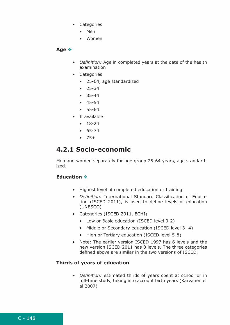
C - 148

• Categories• Men• Women

age v

• Definition: Age in completed years at the date of the health examination

• Categories• 25-64, age standardized• 25-34• 35-44• 45-54• 55-64

• If available• 18-24• 65-74• 75+

4.2.1 Socio-economic

Men and women separately for age group 25-64 years, age standard-ized.

Education v

• Highest level of completed education or training• Definition: International Standard Classification of Educa-

tion (ISCED 2011), is used to define levels of education (UNESCO)

• Categories (ISCED 2011, ECHI)• Low or Basic education (ISCED level 0-2)• Middle or Secondary education (ISCED level 3 -4)• High or Tertiary education (ISCED level 5-8)

• Note: The earlier version ISCED 1997 has 6 levels and the new version ISCED 2011 has 8 levels. The three categories defined above are similar in the two versions of ISCED.

thirds of years of education

• Definition: estimated thirds of years spent at school or in full-time study, taking into account birth years (Karvanen et al 2007)

C - 149

labour (employment) status v

• Definition: Person’s own perception of his/her main activity at present

• Categories• Employed (carrying out a job or profession, including un-

paid work)• unemployed• others (student, retired, military or community service,

domestic tasks, other inactive persons)

living as a couple

• Definition: de facto arrangement, including those who are legally married, living in consensual union or registered partnership

• Categories:• yes• no

Household’s income (equivalised disposable income)

• Definition: Equivalised disposable income is the total in-come of a household, after tax and other deductions, that is available for spending or saving, divided by the number of household members converted into equalised adults; household members are equalised or made equivalent by weighting each according to their age, using the so-called modified OECD equivalence scale(Eurostat). The modified OECD equivalence scale (Hagernaas et al. 1994) gives the following weigths for the members of a household:• 1.0 to the first adult;• 0.5 to the second adult and each subsequent person

aged 14 and over; and• 0.3 to each child aged under 14.

• Categories• Five categories. These are approximately fifths of the

distribution of the equivalised income in each survey. Details of the derivation of the categories are given in the Appendix 5e.

• Comment: Information about children under 14 was not available in the questionnaire used in the EHES Pilot Project, but it was added to the current version of the EHES ques-tionnaire. The analysis of the EHES Pilot Project data used a measure for equivalised disposable income where the total income was divided by the square root of the household’s size (OECD 2008).

C - 150

references• Eurostat modified OECD scale, available at http://ec.europa.eu/eurostat/

statistics-explained/index.php/Glossary:Equivalised_disposable_income• Massimo Piepoli F, Hoes AW, Agewall S et al. 2016 European Guidelines on

cardiovascular disease prevention in clinical practice. The Sixth Joint Task Force of the European Society of Cardiology and Other Societies on Cardio-vascular Disease Prevention in Clinical Practice (constituted by representa-tives of 10 societies and by invited experts). Eur Heart J. 2016;37:2315-81.

• Hagenaars A, de Vos K, Zaidi MA. Poverty statistics in the late 1980s: re-search based on micro-data, Office for official publications of the European communities. Luxemburg, 1994.

• International Diabetes Federation, Clinical Guidelines Task Force. Global guideline for type 2 diabetes, 2012. Available from: http://www.idf.org/sites/default/files/IDF-Guideline-for-Type-2-Diabetes.pdf

• Karvanen J, Veronesi G, Kuulasmaa K. Defining thirds of schooling years in population studies. Eur J Epidemiol. 2007;22(8):487-92. Epub 2007 Jun 13.

• OECD. Growing unequal? Income distribution and poverty in OECD coun-tries, Paris. 2008. Available from http://www.oecd-ilibrary.org/social-is-sues-migration-health/growing-unequal_9789264044197-en

• UNESCO (1997). International Standard Classification of Education ISCED. Available from http://www.uis.unesco.org/Library/Documents/isced97-en.pdf

• UNESCO (2012): International Standard Classification of Education - ISCED 2011. UNESCO Institute for Statistics, Montreal. 2012. Available from: http://www.uis.unesco.org/Education/Documents/isced-2011-en.pdf

• WHO (1995) Physical status: the use and interpretation of anthropometry. Report of a WHO Expert Committee. WHO Technical Report Series 854. Geneva: World Health Organization, 1995. Available from http://apps.who.int/iris/handle/10665/37003

• WHO (2000) Obesity: preventing and managing the global epidemic. Re-port of a WHO Consultation. WHO Technical Report Series 894. Geneva: World Health Organization, 2000. Available from http://apps.who.int/iris/handle/10665/42330

• WHO (2004) WHO Expert consultation. Appropriate body-mass index for Asian populations and its implications for policy and intervention strate-gies. The Lancet, 2004; 157-163

• WHO (2006) Definition and diagnosis of diabetes mellitus and intermediate hyperglycaemia. Report of the WHO/IDF consultation. World Health Organi-zation, 2006. Available from http://apps.who.int/iris/handle/10665/43588

• WHO (2011a) Use of glycated haemoglobin (HbA1c) in the diagnosis of diabetes mellitus. Abbreviated report of a WHO consultation. World Health Organization 2011. Available from http://apps.who.int/iris/han-dle/10665/70523

• WHO (2011b) Waist circumference and waist-hip ration. Report of a WHO Expert Consultation. Geneva, World Health Organization, 2011. Available from http://apps.who.int/iris/handle/10665/44583

• WHO (2013) Global action plan for the prevention and control of noncom-municable diseases 2013-2020. World Health Organization 2013. Available from: http://apps.who.int/iris/handle/10665/94384

Part C


C - 151


During the EHES Pilot Project in 2009-2012, EHES database and a reporting system for basic reports of the results of the national HESs were established in the EHES Reference Centre (EHES RC). This chap-ter describes the outline of the basic report, the established reporting system and principles of estimating the indicators.

5.1 outline of the basic reportEHES basic reporting includes both country-specific and European level reports on survey results. The template of the basic report is provided in Appendix 5a . The basic report includes relevant information about the background and conducting of HESs, description of the used meth-ods and health indicator results.

5.2 reporting systemFor the European level basic reporting, age standardized indicators by sex and age-group are calculated for each survey using HES data in the central EHES database by statistical package R (R Development Core Team 2011). Results on the indicators are saved in the database. The reporting system calculates individual based derived variables and estimates population level indicators by sex and age. Specification of the derived variables used in the basic reporting can be found in Ap-pendix 5b. Technical definitions of the calculation of the indicators are specified in Appendix 5c. Programme codes for executing the reporting can be found in Appendix 5d.

The derived variables are defined using the survey data items specified in the data transfer format in EHES Manual, Part C, Chapter 2. They are calculated for each individual and saved in the EHES database.

The population level indicators are estimated for each survey whose HES data are received in the EHES RC. Each indicator estimate is cat-egorized by sex and 10-year age-group for individuals aged 25-64 years. The indicators are saved in the EHES database in a format that can be used easily by different reporting systems.

5. reporting

Tarja Palosaari1, Johan Heldal2, Hanna Tolonen1, Kari Kuulasmaa1

1National Institute for Health and Welfare (THL), Helsinki, Finland2Statistics Norway, Oslo, Norway

C - 152

5.3 Estimation of indicators

5.3.1 introduction

This chapter defines the methods used for estimating the indicators for the EHES basic report. The methods can be applied to national surveys with little modification as long as the surveys have been carried out according to the EHES recommendations. In the EHES RC, the estima-tion was implemented using statistical package R (R Development Core Team 2011).

5.3.2 Weighting

When estimating population indicators from survey samples we need weights. The weights will generally consist of two components.

1. The sampling weights , also called Horwitz-Thomp-son weights are the inverse of the inclusion probabili-ties for the individuals in the survey and should be known for all individuals invited to the survey regardless

of whether they participated or not, . If the value

of a variable x is known for the entire sample, the sum

provides an unbiased estimate of the population to-tal . Here is the entire sample and means that the sum is over all members of the sample. The formula can be applied to any sub-group of the population. The simple formula is an unbiased estimator of the population size and

is an approximately unbiased estimator of the mean . Whereas wi are weights for estimating population totals

act as weights for estimating population means.

2. The non-response weights . These weights are intend as corrections for unit non-response and are usually based on variables known for everyone in the original sample such as sex, age and geographic affiliation in many countries. In some countries education and income are available. The non-response weights expands the net sample consisting of participants to the gross sample of all invitees. They are

C - 153

most often constructed using some kind of post-stratifica-tion or calibration methods so that estimating totals in the gross sample based on the net sample for some of the vari-ables known for the entire gross sample will provide exactly correct figures. Combining the sampling weights and the non-response weights for all participants to pro-vides the final estimation weights.

Item non-response is not accounted for by the weights. However, this is less of a problem when estimating averages than when estimat-ing population totals. Estimation of population totals results in under-estimation if there are missing values. In the estimation of averages, missing values can be discarded both in numerator and denominator and missingness does not produce bias. The estimators of the popula-tion averages have form

where is the set of participants for whom we have non-missing value

of and .

An alternative to calculate weights is to calibrate them to population

totals rather than just gross sample totals. This can be done in one step or in two steps by first calibrating them to gross sample level and then to population level. This requires good statistics at national level for variables that are observed with good quality for all participants. This way more variables may be accessible than the ones we have in the sampling frame. There must also be a balance: too many calibrat-ing variables may twist the original weights so much out of shape that we lose control of how they work.

For comparability of the results between countries, the methods to establish the weights should be the same in all countries. This puts limits on what methods can be used. Another aspect is the used age standardization and estimation separately for men and women. That’s why the use of sex and age for weighting is less interesting: calibra-tions for sex and age will cancel out in the ωi weights. What remains is the adjustment for different participation rates by geographic area (strata in sampling design).

Weighting was not used in the EHES Pilot project.

5.3.3 Estimation

The estimated indicators are age standardized estimates for 25-64-year-old men and women separately using ten year age groups. If the mean for age-group a (25-34-, 35-44-, 45-54-, 55-64-year-olds) is μa then the age standardized population mean is

C - 154

.

Such an age standardized mean is actually the mean in a hypothetical population where the age distribution is flat. It controls for differential age distribution among the countries and is necessary to make esti-mates comparable across Europe. Also, for comparability over time in later health examination surveys, the age-weights should be kept constant.

Let be the set of respondents in age-group a and let the variable of

interest be . If individual

in the sample belongs to

then it will

have a weight

The parameter is then estimated as

and

5.3.4 imputationThe purpose of imputation is to construct complete data sets that can be analysed without having to exclude records that have missing val-ues on one or more variables so that valuable information is lost. It has also been seen as desirable that analysts should be able to analyse such data sets with standard software as if all data were real and with-out having to pay too much attention to the fact that some of them are imputed.

In survey sampling theory we basically distinguish between two kinds of missing data.

1. unit missing. This includes all individuals that have not participated in the survey and for whom we don’t have any other information than what we could get from the sampling frame.

2. item missing. This is missing on particular variables (ques-tions or measurements) for people who participated at least in parts of the survey.

C - 155

Another aspect of missing data is the statistical mechanism that causes some people to participate and others to say no. Rubin (1976) intro-duced the following distinctions

1. Missing Completely at random (MCar) in relation to a variable means that all individuals have the same probabil-ity of being measured on that variable. For instance, if we observe age for everyone invited to the sample but weight may be missing and the probability that weight is missing is the same for all regardless of age and weight we can say that the data are MCAR.

2. However, if the probability that weight is missing depends on age but not on weight for individuals with the same age we say that weight is Missing at random (Mar).

3. If the probability of weight missing depends on the weight directly, for instance if people who are excessively over-weight do not want to come and hear something they al-ready know very well, then we say that weight is not Miss-ing at random (nMar).

The mechanisms affecting unit missingness and item missingness may be very different. It is likely that missing-mechanisms are NMAR for quite many of the HES variables. Treating NMAR correctly requires a thorough understanding of how the missing mechanisms work to es-tablish a model for doing imputations. Such models will sometimes have to depend on assumptions that are difficult to verify and the in-formation that can be used to estimate such models is often weak. It is often recommended to use the information that is available, pretend that the missing mechanism is MAR and rather evaluate the sensitivity of deviations from the MAR assumption later. Models suggested in this note will assume a MAR mechanism.

Whenever doing imputations, the general practice in survey sampling is to do imputation on items missing but not on unit missing. Unit miss-ing is taken care of by weighting. When imputing a missing value for a specific variable on a record it is, at least in principle, possible to take advantage of the information from other variables that have valid val-ues on the record.

The variables from the sampling frame are often all we have for non-participants. The frame should at least contain information on the ge-ographical affiliation of the sampling unit. If the sampling unit is a household or address a visit to the address may provide information on the number of eligible living there and their distribution with respect to sex and age even if they have not cooperated with the survey. But this will not always be the case. When samples have been taken from registers some kind of information on sex and age, sometimes marital status and other demographic information may come along.

For people participating in the survey we will most often have the in-terview, but we may miss the other measurements. In rarer cases we may have all or some of the other measurements but not the interview.

C - 156

In some of the survey modules, e.g. the interview or anthropometric measurements, some items may be missing while we have others. A question that arises if doing imputations is to which extent we should allow imputations of entire modules based on information from others.

As estimates or predictions of the true missing values, imputations are always uncertain. This uncertainty adds to the sampling uncertainty and uncertainty in measurements. If an imputed data set is analyzed with standard methods not paying attention to the imputation method used, the variance estimates will be underestimated and test will reject too often.

There are several imputation techniques. The oldest ones are the “hot-deck methods” where the records have been grouped according to known variables (age, sex, geography etc.). Then each missing obser-vation is replaced with a value drawn at random among the observed values in the same group. Second, we have nearest neighbour meth-ods which do not require grouping but sorting and there are mean and regression imputation methods. Regression imputation can be carried out deterministically by replacing the missing value with a predicted one. Alternatively a randomly drawn regression residual can be added to reflect prediction uncertainty.

Multiple imputation where several values are imputed for one missing value goes back to Rubin 1978. The purpose of multiple imputation is to have the imputation uncertainty reflected in the data. Rubin devised a variance formula which should take care of the imputation uncer-tainty in a correct manner. However, for Rubin’s formula to be correct the imputation has to be ‘proper’. This means that the imputation must be based on a model for the missing data given the observed data. A prior distribution for the parameters in the model is required and a full Bayesian posterior distribution must be established. Then the imputed values must be drawn from this posterior distribution. Multiple imputa-tion can be done with other methods than that of Rubin. In principle all kinds of stochastic imputation can be carried out multiply.

Imputation was not used in the EHES Pilot project.When imputation is used for the basic reports, the imputed data set(s) must be stored in addition to the original dataset. This makes it possible to reproduce the estimates in the future.

5.3.5 Smoothing

If the estimates for 10 year age-groups are calculated using one year

age groups , each estimate will be based on the small number of

observations that falls in age group . The sequence will therefore behave somewhat erratic, jumping up and down. However, for

many indicators the underlying sequence of true values

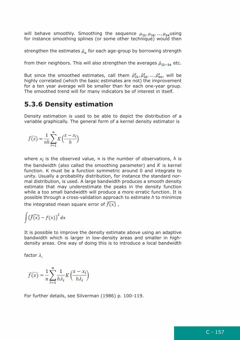
C - 157

will behave smoothly. Smoothing the sequence using for instance smoothing splines (or some other technique) would then

strengthen the estimates for each age-group by borrowing strength

from their neighbors. This will also strengthen the averages etc.

But since the smoothed estimates, call them , will be highly correlated (which the basic estimates are not) the improvement for a ten year average will be smaller than for each one-year group. The smoothed trend will for many indicators be of interest in itself.

5.3.6 Density estimation

Density estimation is used to be able to depict the distribution of a variable graphically. The general form of a kernel density estimator is

where xi is the observed value, is the number of observations, is the bandwidth (also called the smoothing parameter) and is kernel function. K must be a function symmetric around 0 and integrate to unity. Usually a probability distribution, for instance the standard nor-mal distribution, is used. A large bandwidth produces a smooth density estimate that may underestimate the peaks in the density function while a too small bandwidth will produce a more erratic function. It is possible through a cross-validation approach to estimate h to minimize the integrated mean square error of ,

It is possible to improve the density estimate above using an adaptive bandwidth which is larger in low-density areas and smaller in high-density areas. One way of doing this is to introduce a local bandwidth

factor

For further details, see Silverman (1986) p. 100-119.

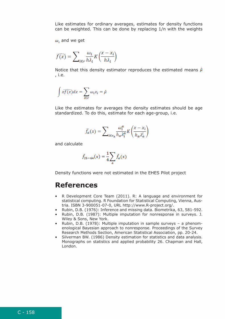
C - 158

Like estimates for ordinary averages, estimates for density functions can be weighted. This can be done by replacing 1/n with the weights

and we get

Notice that this density estimator reproduces the estimated means , i.e.

Like the estimates for averages the density estimates should be age standardized. To do this, estimate for each age-group, i.e.

and calculate

Density functions were not estimated in the EHES Pilot project

references• R Development Core Team (2011). R: A language and environment for

statistical computing. R Foundation for Statistical Computing, Vienna, Aus-tria. ISBN 3-900051-07-0, URL http://www.R-project.org/.

• Rubin, D.B. (1976): Inference and missing data. Biometrika, 63, 581-592.• Rubin, D.B. (1987): Multiple imputation for nonresponse in surveys. J.

Wiley & Sons, New York.• Rubin, D.B. (1978): Multiple imputation in sample surveys – a phenom-

enological Bayesian approach to nonresponse. Proceedings of the Survey Research Methods Section, American Statistical Association, pp. 20-24.

• Silverman BW. (1986) Density estimation for statistics and data analysis. Monographs on statistics and applied probability 26. Chapman and Hall, London.

C - 159

appendix 5a. template of the basic report

• Introduction• Background

• What is known about previous health surveys?• What is known or not known about health status based

on existing data sources and previous surveys?• Survey aims

• Why survey is conducted?• Target population and sampling

• Which population groups are covered and which are not covered by target population?

• How the sampling was conducted and which sampling frames were used?

• Sample characteristics and participation rates (incl. eligibil-ity) by sex and 10-year age groups• Tablel1. Proportion of eligibles, Proportion of not-con-

tacted, Proportion of non-eligible• Table 2. Proportion of participants

• questionnaire only• examination only• both

• Table 3. Proportion of non-participants• Data collection methods

• How data was collected?• Questionnaire administration

• Use of proxies (if used)• Measurement procedures

• Analysis• What kind of weighting was used?• Sub-groups used for reporting

• Results• Rationale for each indicator• Definition of the indicator• Table with results by sex and 10-year age group, age

standardized 25-64• Summary of the results by indicator, including notes if

known that data has some problems, shortcomings or special features.

• Background items• Area

C - 160

• Sex• Age• Education• Labour (employment) status

• Health indicators• Blood pressure

• Systolic blood pressure: Population mean, stand-ard error and 95 % confidence interval

• Diastolic blood pressure: Population mean, stand-ard error and 95 % confidence interval

• Prevalence of self-reported high blood pressure (hypertension) (%)

• Prevalence of actual and potential hypertensives (%)

• Awareness of elevated blood pressure among ac-tual and potential hypertensives (%)

• Prevalence of anti-hypertensive drug use in the population (%)

• Prevalence of anti-hypertensive drug use among actual and potential hypertensives (%)

• Prevalence of optimal blood pressure among those using anti-hypertensive drugs (%)

• Proportion of the population with blood pressure measurement in the past 5 years (%)

• Lipids• Serum total cholesterol: Population mean, stand-

ard error and 95 % confidence interval• Serum high-density lipoprotein cholesterol: Popu-

lation mean, standard error and 95 % confidence interval

• Serum non-HDL cholesterol: Population mean, standard error and 95 % confidence interval

• Prevalence of self-reported elevated blood choles-terol (%)

• Prevalence of actual or potential elevated serum total cholesterol in the population (%)

• Prevalence of lipid lowering drug use in the popu-lation (%)

• Prevalence of lipid lowering drug use among those with elevated total cholesterol (%)

• Prevalence of optimal total cholesterol level among those using lipid lowering drugs (%)

• Proportion of the population with cholesterol measurement in the past 5 years (%)

• Glucose

C - 161

• Fasting plasma glucose: Population mean, stand-ard error and 95 % confidence interval

• Glycated haemoglobin (HbA1c): Population mean, standard error and 95 % confidence interval

• Prevalence of self-reported diabetes (%)• Prevalence of diabetes (%) based on fasting glu-

cose, HbA1c or use of diabetes medication• Prevalence of diabetes medication in population

(%)• Prevalence of diabetes medication among actual

and potential diabetics (%)• Awareness of diabetes among diabetics (%)• Prevalence of the population with blood glucose

measured in the past 5 years (%)• Anthropometric measurements

• Waist circumference: Population mean, standard error and 95 % confidence interval

• BMI (measured): Population mean, standard error and 95 % confidence interval

• BMI self-reported: Population mean, standard er-ror and 95 % confidence interval

• Prevalence of overweight (%) based on measured BMI

• Prevalence of obesity (%) based on measured BMI• Categories of waist circumference

• Self-perceived health and chronic diseases• Self-perceived health• Prevalence of self-reported chronic morbidity (%)• Prevalence of long-term activity limitations (%)• Prevalence of self-reported myocardial infarction

(%)• Prevalence of self-reported coronary heart disease

(%)• Prevalence of self-reported stroke (%)

• Smoking• Prevalence of daily smokers (%)• Prevalence of ex-daily smokers (%)

C - 162

Appendix 5b. Specification of derived variablesDefinitions of variables transferred to EHES RC can be found in EHES Manual, Part C, Chapter 2. Further information and program codes for calculation of derived variables, see the Appendix 5d.

Abbreviations:!= not equal.

background items

ColuMn naME tYPE DEFinition

EDUCATION_CAT integer Highest education leaving certificate obtained: 1 = Low or Basic education (ISCED level 0-2), if EDUCATION = 1 or 2 or 3. 2 = Middle or Secondary education (ISCED level 3-4), if EDUCATION = 4 or 5. 3 = High or Tertiary education (ISCED level 5-6), if EDUCATION = 6 or 7. 9 = Missing data if EDUCATION = 9.

LABOUR_CAT integer Current labour (employment) status: 1 = Employed (carrying out a job or profession, including unpaid work), if LABOUR_STATUS = 1. 2 = Unemployed, if LABOUR_STATUS = 2. 3 = Other (student, retired, military or community service, domestic tasks, other inactive persons), if LABOUR_STATUS = 3 or 4 or 5 or 6 or 7 or 8. 9 = Missing data if LABOUR_STATUS = 9.

EMPLOYMENT1 integer Employee, self-employed or working without payment as a family worker: 1 = Employe if PROFIT = 1 and EMPLOYMENT = 1. 2 = Self-employe if PROFIT = 1 and EMPLOYMENT = 2. 3 = Family worker if PROFIT = 1 and EMPLOYMENT = 3. 9 = Missing data if PROFIT = 1 and EMPLOYMENT = 9. . = irrelevant if PROFIT != 1.

C - 163

blood pressure


BP_SYSTM23 decimal (0.01)

Systolic blood pressure (mmHg), 2nd and 3rd measurement. If EXAM = 1 or QUEST = 1: Mean of BP_SYST2 and BP_SYST3. 999.99 (missing) if EXAM = 2 or BP_SYST2 = 999 or BP_SYST3 = 999.


Systolic blood pressure (mmHg), 1st and 2nd measurement. If EXAM = 1 or QUEST = 1: Mean of BP_SYST1 and BP_SYST1. 999.99 (missing) if EXAM = 2 or BP_SYST1 = 999 or BP_SYST2 = 999.


Systolic blood pressure (mmHg), 1st, 2nd and 3rd measurement. If EXAM = 1 or QUEST = 1: Mean of BP_SYST1, BP_SYST2 and BP_SYST3. 999.99 (missing) if EXAM = 2 or BP_SYST1 = 999 or BP_SYST2 = 999 or BP_SYST3 = 999.

BP_DIASTM23 decimal (0.01)

Diastolic blood pressure (mmHg), 2nd and 3rd measurement. If EXAM = 1 or QUEST = 1: Mean of BP_DIAST2 and BP_DIAST3. 999.99 (missing) if EXAM = 2 or BP_DIAST2 = 999 or BP_DIAST3 = 999.


Diastolic blood pressure (mmHg), 1st and 2nd measurement. If EXAM = 1 or QUEST = 1: Mean of BP_DIAST1 and BP_DIAST2. 999.99 (missing) if EXAM = 2 or (BP_DIAST1 = 999 or BP_DIAST2 = 999).


Diastolic blood pressure (mmHg), 1st, 2nd and 3rd measurement. If EXAM = 1 or QUEST = 1: Mean of BP_DIAST1, BP_DIAST2 and BP_DIAST3 if ELIG = 1 and EXAM = 1. 999.99 (missing) if EXAM = 2 or (BP_DIAST1 = 999 or BP_DIAST2 = 999 or BP_DIAST3 = 999).

BP_SYST decimal (0.01)

Systolic blood pressure (mmHg). If EXAM = 1 or QUEST = 1: BP_SYSTM23 if not missing, then BP_SYSTM12 if not missing, then BP_SYST2 if not missing, then BP_SYST3 if not missing, then BP_SYST1 if not missing, then 999.99 (missing) if EXAM = 2 or BP_SYST1 = BP_SYST2 = BP_SYST3 = 999 (missing).

C - 164


BP_DIAST decimal (0.01)

Diastolic blood pressure (mmHg). If EXAM = 1 or QUEST = 1: BP_DIASTM23 if not missing, then BP_DIASTM12 if not missing, then BP_DIAST2 if not missing, then BP_DIAST3 if not missing, then BP_DIAT1 if not missing, then 999.99 (missing) if EXAM = 2 or BP_DIAST1 = BP_DIAST2 = BP_DIAST3 = 999 (missing).

Hypertension:

MEDICINE_HBP1 integer Medicines for high blood pressure. If MEDICINE = 1 and (EXAM = 1 or QUEST = 1): 1 (yes) if MEDICINE = 1 and MEDICINE_HBP = 1. 2 (no) if ((MEDICINE = 1 and MEDICINE_HBP = 2). 9 (missing) if QUEST = 2 or (MEDICINE = 1 and MEDICINE_HBP != 1 and MEDICINE_HBP != 2). . (irrelevant) if MEDICINE != 1.

MEDICINE_HBP_POP integer Medicines for high blood pressure among population. If EXAM = 1 or QUEST = 1: 1 (yes) if MEDICINE_HBP1 = 1. 2 (no) if MEDICINE = 2 or MEDICINE_HBP1 = 2. 9 (missing) if QUEST = 2 or (MEDICINE = 1 and MEDICINE_HBP1 = 9) or MEDICINE != (1 and 2) .

BP_HBP integer Actual or potential hypertension. If EXAM = 1 or QUEST = 1: 1 (yes) if none of 3 is missing and (BP_SYST >= 140 or BP_DIAST >= 90 or MEDICINE_HBP1 = 1). 2 (no) if none of 3 is missing and (BP_SYST < 140 and BP_DIAST < 90 and MEDICINE_HBP1 = 2). 9 (missing) if EXAM = 2 or QUEST = 2 or BP_SYST = missing or BP_DIAST = missing or (MEDICINE_HBP1 != 1 and MEDICINE_HBP1 != 2).

C - 165


MEDICINE_HBP_ILL integer Medicines for high blood pressure among actual or potential hypertensives. If EXAM = 1 or QUEST = 1: 1 (yes) if BP_HBP = 1 and MEDICINE_HBP1 = 1. 2 (no) if (BP_HBP = 1 and MEDICINE_HBP1 = 2) or (BP_HBP = 1 and MEDICINE = 2). 9 (missing) if BP_HBP = 1 and (MEDICINE_HBP1 = 9 or MEDICINE = 9). . (irrelevant) if BP_HBP != 1.

BP_AWARE integer Awareness of hypertension among actual or potential hypertensives. If EXAM = 1 or QUEST = 1: 1 (yes) if BP_HBP = 1 and DIAGN_HBP = 1. 2 (no) if BP_HBP = 1 and (DIAGN_HBP =2 or DIAGN_HBP = 8). 9 (missing) if BP_HBP = 1 and DIAGN_HBP != 1 and DIAGN_HBP != 2 and DIAGN_HBP != 8. . (irrelevant) if BP_HBP != 1.

BP_OPTIMAL integer Optimal blood pressure among those using anti-hypertensive drugs. If EXAM = 1 or QUEST = 1: 1 (yes) if MEDICINE_HBP1 = 1 and BP_EPB = 2. 2 (no) if MEDICINE_HBP1 = 1 and BP_EPB = 1. 9 (missing) if MEDICINE_HBP1 = 1 and BP_EPB != 1 and BP_EPB != 2. . (irrelevant) if MEDICINE_HBP1 != 1.

lipids


BS_CHOL_MMOL decimal 0.0001

Serum total cholesterol in mmol/l. If EXAM = 1 or QUEST = 1: BS_CHOL if BS_UNIT_CHOL= 1. BS_CHOL divided by 38.67 if BS_UNIT_CHOL= 2. 9999.9999 (missing) if EXAM = 2 or BS_CHOL = 9999.99.

BS_HDL_MMOL decimal Serum HDL cholesterol in mmol/l. If EXAM = 1 or QUEST = 1: BS_HDL if BS_UNIT_HDL = 1 . BS_HDL divided by 38.67 if BS_UNIT_HDL = 2. 9999.9999 (missing) if EXAM = 2 or BS_HDL = 9999.99.

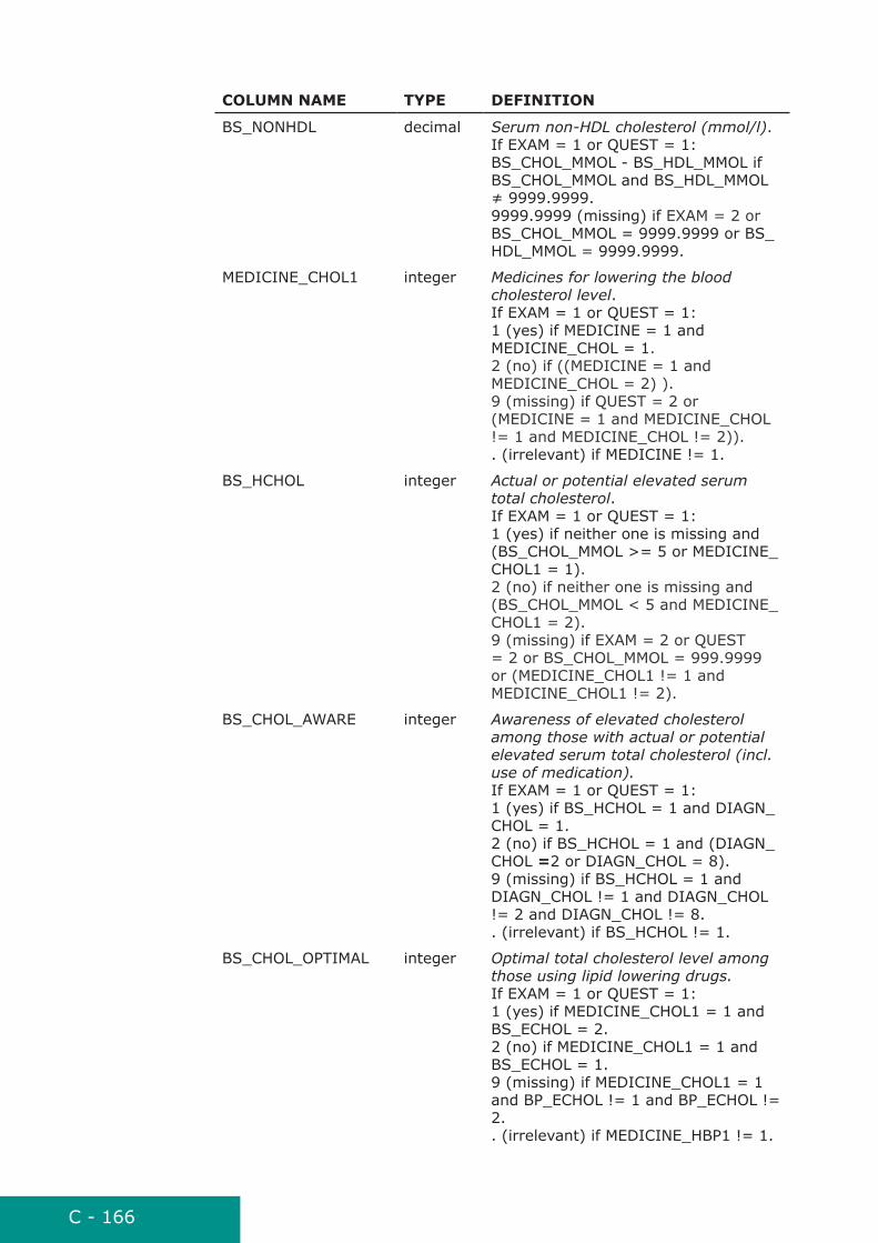
C - 166


BS_NONHDL decimal Serum non-HDL cholesterol (mmol/l). If EXAM = 1 or QUEST = 1: BS_CHOL_MMOL - BS_HDL_MMOL if BS_CHOL_MMOL and BS_HDL_MMOL ≠ 9999.9999. 9999.9999 (missing) if EXAM = 2 or BS_CHOL_MMOL = 9999.9999 or BS_HDL_MMOL = 9999.9999.

MEDICINE_CHOL1 integer Medicines for lowering the blood cholesterol level. If EXAM = 1 or QUEST = 1: 1 (yes) if MEDICINE = 1 and MEDICINE_CHOL = 1. 2 (no) if ((MEDICINE = 1 and MEDICINE_CHOL = 2) ). 9 (missing) if QUEST = 2 or (MEDICINE = 1 and MEDICINE_CHOL != 1 and MEDICINE_CHOL != 2)). . (irrelevant) if MEDICINE != 1.

BS_HCHOL integer Actual or potential elevated serum total cholesterol. If EXAM = 1 or QUEST = 1: 1 (yes) if neither one is missing and (BS_CHOL_MMOL >= 5 or MEDICINE_CHOL1 = 1). 2 (no) if neither one is missing and (BS_CHOL_MMOL < 5 and MEDICINE_CHOL1 = 2). 9 (missing) if EXAM = 2 or QUEST = 2 or BS_CHOL_MMOL = 999.9999 or (MEDICINE_CHOL1 != 1 and MEDICINE_CHOL1 != 2).

BS_CHOL_AWARE integer Awareness of elevated cholesterol among those with actual or potential elevated serum total cholesterol (incl. use of medication). If EXAM = 1 or QUEST = 1: 1 (yes) if BS_HCHOL = 1 and DIAGN_CHOL = 1. 2 (no) if BS_HCHOL = 1 and (DIAGN_CHOL =2 or DIAGN_CHOL = 8). 9 (missing) if BS_HCHOL = 1 and DIAGN_CHOL != 1 and DIAGN_CHOL != 2 and DIAGN_CHOL != 8. . (irrelevant) if BS_HCHOL != 1.

BS_CHOL_OPTIMAL integer Optimal total cholesterol level among those using lipid lowering drugs. If EXAM = 1 or QUEST = 1: 1 (yes) if MEDICINE_CHOL1 = 1 and BS_ECHOL = 2. 2 (no) if MEDICINE_CHOL1 = 1 and BS_ECHOL = 1. 9 (missing) if MEDICINE_CHOL1 = 1 and BP_ECHOL != 1 and BP_ECHOL != 2. . (irrelevant) if MEDICINE_HBP1 != 1.

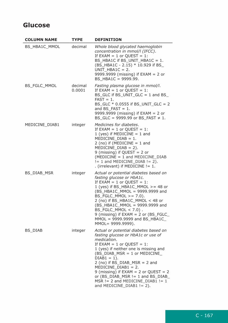
C - 167

Glucose


BS_HBA1C_MMOL decimal Whole blood glycated haemoglobin concentration in mmol/l (IFCC). If EXAM = 1 or QUEST = 1: BS_HBA1C if BS_UNIT_HBA1C = 1. (BS_HBA1C - 2.15) * 10.929 if BS_UNIT_HBA1C = 2. 9999.9999 (missing) if EXAM = 2 or BS_HBA1C = 9999.99.

BS_FGLC_MMOL decimal 0.0001

Fasting plasma glucose in mmol/l. If EXAM = 1 or QUEST = 1: BS_GLC if BS_UNIT_GLC = 1 and BS_FAST = 1. BS_GLC * 0.0555 if BS_UNIT_GLC = 2 and BS_FAST = 1. 9999.9999 (missing) if EXAM = 2 or BS_GLC = 9999.99 or BS_FAST ≠ 1.

MEDICINE_DIAB1 integer Medicines for diabetes. If EXAM = 1 or QUEST = 1: 1 (yes) if MEDICINE = 1 and MEDICINE_DIAB = 1. 2 (no) if (MEDICINE = 1 and MEDICINE_DIAB = 2). 9 (missing) if QUEST = 2 or (MEDICINE = 1 and MEDICINE_DIAB != 1 and MEDICINE_DIAB != 2). . (irrelevant) if MEDICINE != 1.

BS_DIAB_MSR integer Actual or potential diabetes based on fasting glucose or HbA1c. If EXAM = 1 or QUEST = 1: 1 (yes) if BS_HBA1C_MMOL >= 48 or (BS_HBA1C_MMOL = 9999.9999 and BS_FGLC_MMOL >= 7.0). 2 (no) if BS_HBA1C_MMOL < 48 or (BS_HBA1C_MMOL = 9999.9999 and BS_FGLC_MMOL < 7.0) . 9 (missing) if EXAM = 2 or (BS_FGLC_MMOL = 9999.9999 and BS_HBA1C_MMOL= 9999.9999).

BS_DIAB integer Actual or potential diabetes based on fasting glucose or HbA1c or use of medication. If EXAM = 1 or QUEST = 1: 1 (yes) if neither one is missing and (BS_DIAB_MSR = 1 or MEDICINE_DIAB1 = 1). 2 (no) if BS_DIAB_MSR = 2 and MEDICINE_DIAB1 = 2. 9 (missing) if EXAM = 2 or QUEST = 2 or (BS_DIAB_MSR != 1 and BS_DIAB_MSR != 2 and MEDICINE_DIAB1 != 1 and MEDICINE_DIAB1 != 2).

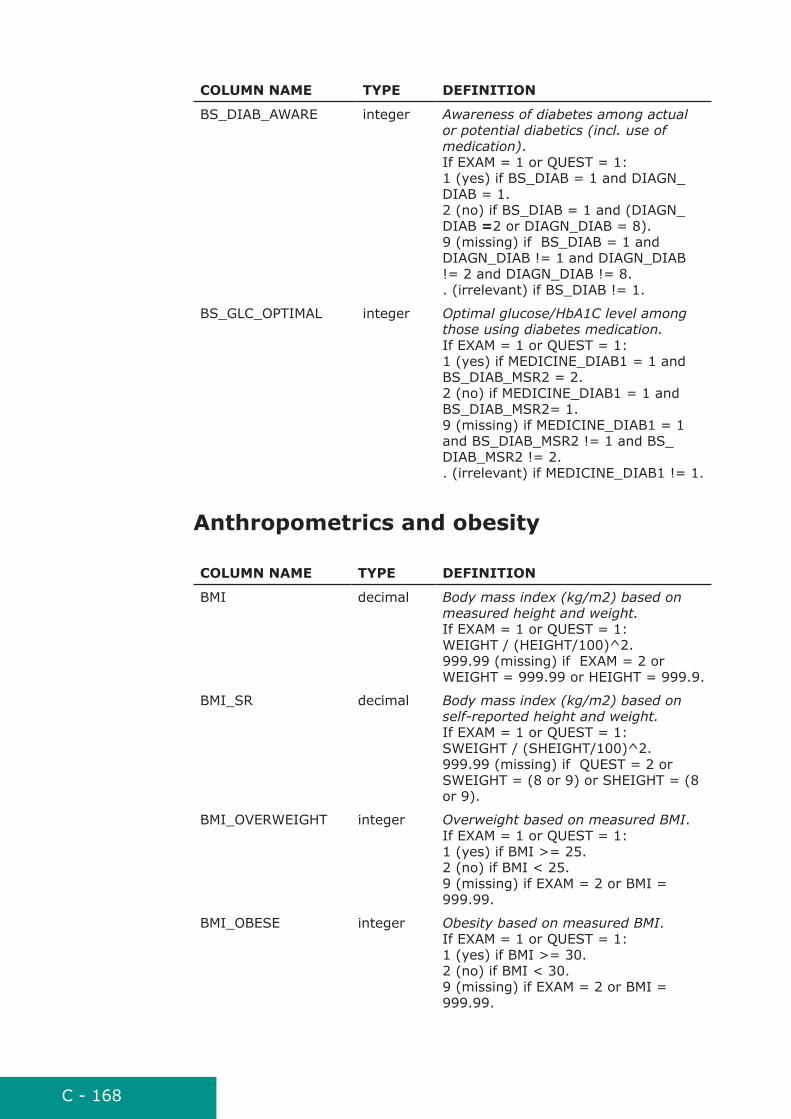
C - 168


BS_DIAB_AWARE integer Awareness of diabetes among actual or potential diabetics (incl. use of medication). If EXAM = 1 or QUEST = 1: 1 (yes) if BS_DIAB = 1 and DIAGN_DIAB = 1. 2 (no) if BS_DIAB = 1 and (DIAGN_DIAB =2 or DIAGN_DIAB = 8). 9 (missing) if BS_DIAB = 1 and DIAGN_DIAB != 1 and DIAGN_DIAB != 2 and DIAGN_DIAB != 8. . (irrelevant) if BS_DIAB != 1.

BS_GLC_OPTIMAL integer Optimal glucose/HbA1C level among those using diabetes medication. If EXAM = 1 or QUEST = 1: 1 (yes) if MEDICINE_DIAB1 = 1 and BS_DIAB_MSR2 = 2. 2 (no) if MEDICINE_DIAB1 = 1 and BS_DIAB_MSR2= 1. 9 (missing) if MEDICINE_DIAB1 = 1 and BS_DIAB_MSR2 != 1 and BS_DIAB_MSR2 != 2. . (irrelevant) if MEDICINE_DIAB1 != 1.

anthropometrics and obesity


BMI decimal Body mass index (kg/m2) based on measured height and weight. If EXAM = 1 or QUEST = 1: WEIGHT / (HEIGHT/100)^2. 999.99 (missing) if EXAM = 2 or WEIGHT = 999.99 or HEIGHT = 999.9.

BMI_SR decimal Body mass index (kg/m2) based on self-reported height and weight. If EXAM = 1 or QUEST = 1: SWEIGHT / (SHEIGHT/100)^2. 999.99 (missing) if QUEST = 2 or SWEIGHT = (8 or 9) or SHEIGHT = (8 or 9).

BMI_OVERWEIGHT integer Overweight based on measured BMI. If EXAM = 1 or QUEST = 1: 1 (yes) if BMI >= 25. 2 (no) if BMI < 25. 9 (missing) if EXAM = 2 or BMI = 999.99.

BMI_OBESE integer Obesity based on measured BMI. If EXAM = 1 or QUEST = 1: 1 (yes) if BMI >= 30. 2 (no) if BMI < 30. 9 (missing) if EXAM = 2 or BMI = 999.99.

C - 169


WAIST_LARGE integer Large waist circumference. If EXAM = 1 or QUEST = 1: 1 (yes) if (SEX = 1 (male) and WAIST > 102) or (SEX = 2 (female) and WAIST > 88). 2 (no) if (SEX = 1 and WAIST <= 102) or (SEX = 2 and WAIST <= 88). 9 (missing) if EXAM = 2 or WAIST = 999.9 or (SEX != 1 and SEX != 2).

Self-perceived health


HEALTH_GOOD integer Self perceived health at least good. If EXAM = 1 or QUEST = 1: 1 (yes) if HEALTH = 1 or 2. 2 (no) if HEALTH = 3 or 4 or 5. 8 (don’t know) if HEALTH = 8. 9 (missing) if QUEST = 2 or HEALTH = 9.

LIMITED_YES integer Long-term activity limitations due to health problems. If EXAM = 1 or QUEST = 1: 1 (yes) if LIMITED = 1 or 2. 2 (no) if LIMITED = 3. 8 (don’t know) if LIMITED = 8. 9 (missing) if QUEST = 2 or LIMITED = 9.

Specification of additional derived vari-ables

Further information and program codes for calculation of derived variables, see the Appendix 5d.

Questionnaire items


SCHOOL_THIRDS integer Thirds of years of education. Derived from BIRTH_YEAR, SCHOOL_YEAR. Reference: J. Karvanen, G. Veronesi, K. Kuulasmaa (2007). Defining thirds of schooling years in population studies. European Journal of Epidemiology, Volume 22, Number 8, 487--492.

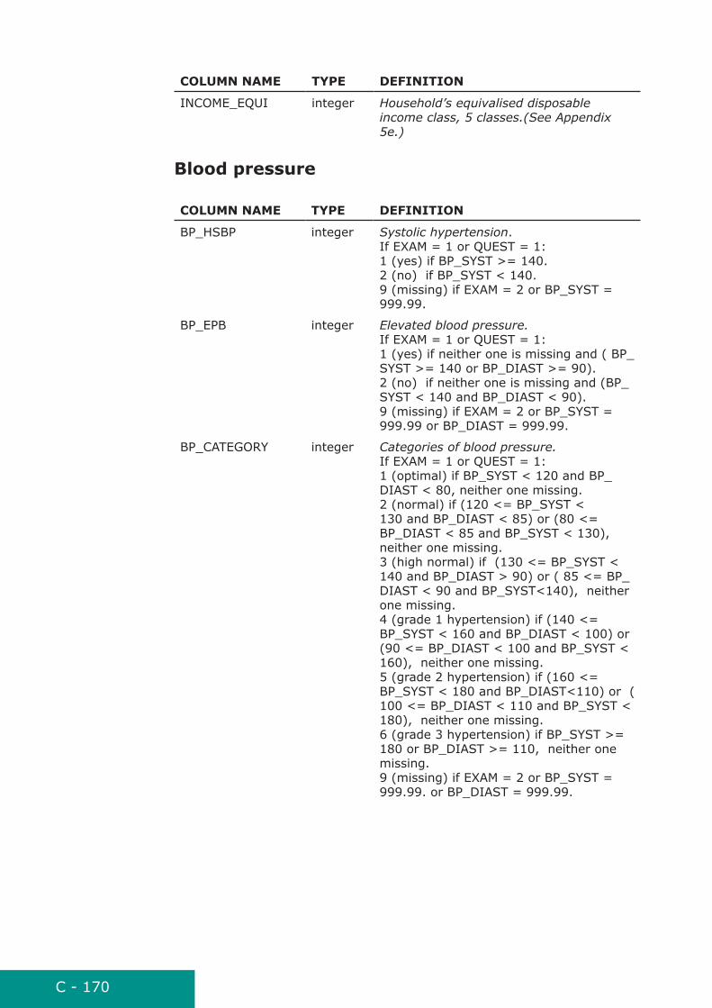
C - 170


INCOME_EQUI integer Household’s equivalised disposable income class, 5 classes.(See Appendix 5e.)

Family_income.docblood pressure


BP_HSBP integer Systolic hypertension. If EXAM = 1 or QUEST = 1: 1 (yes) if BP_SYST >= 140. 2 (no) if BP_SYST < 140. 9 (missing) if EXAM = 2 or BP_SYST = 999.99.

BP_EPB integer Elevated blood pressure. If EXAM = 1 or QUEST = 1: 1 (yes) if neither one is missing and ( BP_SYST >= 140 or BP_DIAST >= 90). 2 (no) if neither one is missing and (BP_SYST < 140 and BP_DIAST < 90). 9 (missing) if EXAM = 2 or BP_SYST = 999.99 or BP_DIAST = 999.99.

BP_CATEGORY integer Categories of blood pressure. If EXAM = 1 or QUEST = 1: 1 (optimal) if BP_SYST < 120 and BP_DIAST < 80, neither one missing. 2 (normal) if (120 <= BP_SYST < 130 and BP_DIAST < 85) or (80 <= BP_DIAST < 85 and BP_SYST < 130), neither one missing. 3 (high normal) if (130 <= BP_SYST < 140 and BP_DIAST > 90) or ( 85 <= BP_DIAST < 90 and BP_SYST<140), neither one missing. 4 (grade 1 hypertension) if (140 <= BP_SYST < 160 and BP_DIAST < 100) or (90 <= BP_DIAST < 100 and BP_SYST < 160), neither one missing. 5 (grade 2 hypertension) if (160 <= BP_SYST < 180 and BP_DIAST<110) or ( 100 <= BP_DIAST < 110 and BP_SYST < 180), neither one missing. 6 (grade 3 hypertension) if BP_SYST >= 180 or BP_DIAST >= 110, neither one missing. 9 (missing) if EXAM = 2 or BP_SYST = 999.99. or BP_DIAST = 999.99.

C - 171


BP_MEDEFF_HBP integer Effective antihypertensive drug treatment. If EXAM = 1 or QUEST = 1: 1 (yes) if BP_SYST < 140 and BP_DIAST < 90 and MEDICINE_HBP1 = 1. 2 (no) if (neither one is missing and (BP_SYST >= 140 or BP_DIAST >= 90)) and MEDICINE_HBP1 = 1. 9 (missing) if MEDICINE_HBP1 = 1 and (BP_SYST = missing or BP_DIAST = missing). . (irrelevant) if MEDICINE_HBP1 != 1.

lipids


BS_CHOLHDL_RATIO decimal Ratio of serum total cholesterol and HDL cholesterol. If EXAM = 1 or QUEST = 1: BS_CHOL_MMOL divided by BS_HDL_MMOL if BS_CHOL_MMOL and BS_HDL_MMOL ≠ 9999.9999. 9999.9999 (missing) if EXAM = 2 or BS_CHOL_MMOL = 9999.9999 or BS_HDL_MMOL = 9999.9999.

BS_ECHOL6 integer Elevated serum total cholesterol, different cutpoints: 6 mmol/l. If EXAM = 1 or QUEST = 1: 1 (yes) if BS_CHOL_MMOL >= 6. 2 (no) if BS_CHOL_MMOL < 6. 9 (missing) if EXAM = 2 or BS_CHOL_MMOL = 9999.9999.



C - 172


BS_CHOL_CATEGORY

integer Categories of serum total cholesterol. If EXAM = 1 or QUEST = 1: 1 if BS_CHOL_MMOL < 5. 2 if BS_CHOL_MMOL >= 5 and BS_CHOL_MMOL < 6. 3 if BS_CHOL_MMOL >= 6 and BS_CHOL_MMOL < 7. 4 if BS_CHOL_MMOL >= 7 and BS_CHOL_MMOL < 8. 5 if BS_CHOL_MMOL >= 8. 9 (missing) if EXAM = 2 or BS_CHOL_MMOL = 9999.9999

BS_LHDL integer Low serum HDL cholesterol. If EXAM = 1 or QUEST = 1: 1 (yes) if (SEX = 1 (male) and BS_CHOL_MMOL < 1) or (SEX = 2 and BS_CHOL_MMOL < 1.2). 2 (no) if (SEX = 1 and BS_CHOL_MMOL >= 1) or (SEX = 2 and BS_CHOL_MMOL >= 1.2). 9 (missing) if EXAM = 2 or BS_CHOL_MMOL = 9999.9999 or (SEX != 1 and SEX != 2). (empty value), if ELIG ≠ 1 or EXAM = 2.

BS_HRATIO integer High serum total cholesterol to HDL cholesterol ratio. If EXAM = 1 or QUEST = 1: 1 (yes) if BS_CHOLHDL_RATIO > 5. 2 (no) if BS_CHOLHDL_RATIO <= 5. 9 (missing) if EXAM = 2 or BS_CHOLHDL_RATIO = 9999.9999.

BS_ECHOL integer Elevated serum total cholesterol. If EXAM = 1 or QUEST = 1: 1 (yes) if BS_CHOL_MMOL >= 5 . 2 (no) if BS_CHOL_MMOL < 5. 9 (missing) if EXAM = 2 or BS_CHOL_MMOL = 9999.9999.

BS_ENONHDL integer Elevated non-HDL cholesterol. If EXAM = 1 or QUEST = 1: 1 (yes) if BS_NONHDL > 3.5. 2 (no) if BS_NONHDL <= 3.5. 9 (missing) if EXAM = 2 or BS_NONHDL = 9999.9999.

C - 173


BS_HNONHDL integer Actual or potential elevated non-HDL cholesterol. If EXAM = 1 or QUEST = 1: 1 (yes) if neither one is missing and ( BS_NONHDL > 3.5 or MEDICINE_CHOL1 = 1) . 2 (no) if neither one is missing and (BS_NONHDL <= 3.5 and MEDICINE_CHOL1 = 2). 9 (missing) if EXAM = 2 or QUEST = 2 or BS_NONHDL = 9999.9999 or (MEDICINE_CHOL1 != 1 and MEDICINE_CHOL1 != 2).

BS_MEDEFF_CHOL integer Effective cholesterol treatment. If EXAM = 1 or QUEST = 1: 1 (yes) if BS_CHOL_MMOL < 5 and MEDICINE_CHOL1 = 1. 2 (no) if BS_CHOL_MMOL >= 5 and MEDICINE_CHOL1 = 1. 9 (missing) if MEDICINE_CHOL1 = 1 and BS_CHOL_MMOL = 9999.9999. . (irrelevant) if MEDICINE_CHOL1 != 1.

Glucose


BS_GLYCEMIA integer Provisional diagnosis of impaired fasting glucose (IFG). If EXAM = 1 or QUEST = 1: 1 (yes) if 6.0 < BS_FGLC_MMOL < 7.0. 2 (no) if BS_FGLC_MMOL <= 6.0 or BS_FGLC_MMOL >= 7.0. 9 (missing) if EXAM = 2 or BS_FGLC_MMOL = 9999.9999.

BS_PROVDIAB_GLC integer Provisional diagnosis of diabetes based on fasting plasma glucose. If EXAM = 1 or QUEST = 1: 1 (yes) if BS_FGLC_MMOL >= 7.0. 2 (no) if BS_FGLC_MMOL < 7.0. 9 (missing) if EXAM = 2 or BS_FGLC_MMOL = 9999.9999.


BS_PROVDIAB_HBA1C

integer Provisional diagnosis of diabetes based on HbA1c. If EXAM = 1 or QUEST = 1: 1 (yes) if BS_HBA1C_MMOL >= 48. 2 (no) if BS_HBA1C_MMOL < 48. 9 (missing) if EXAM = 2 or BS_HBA1C_MMOL = 9999.9999.

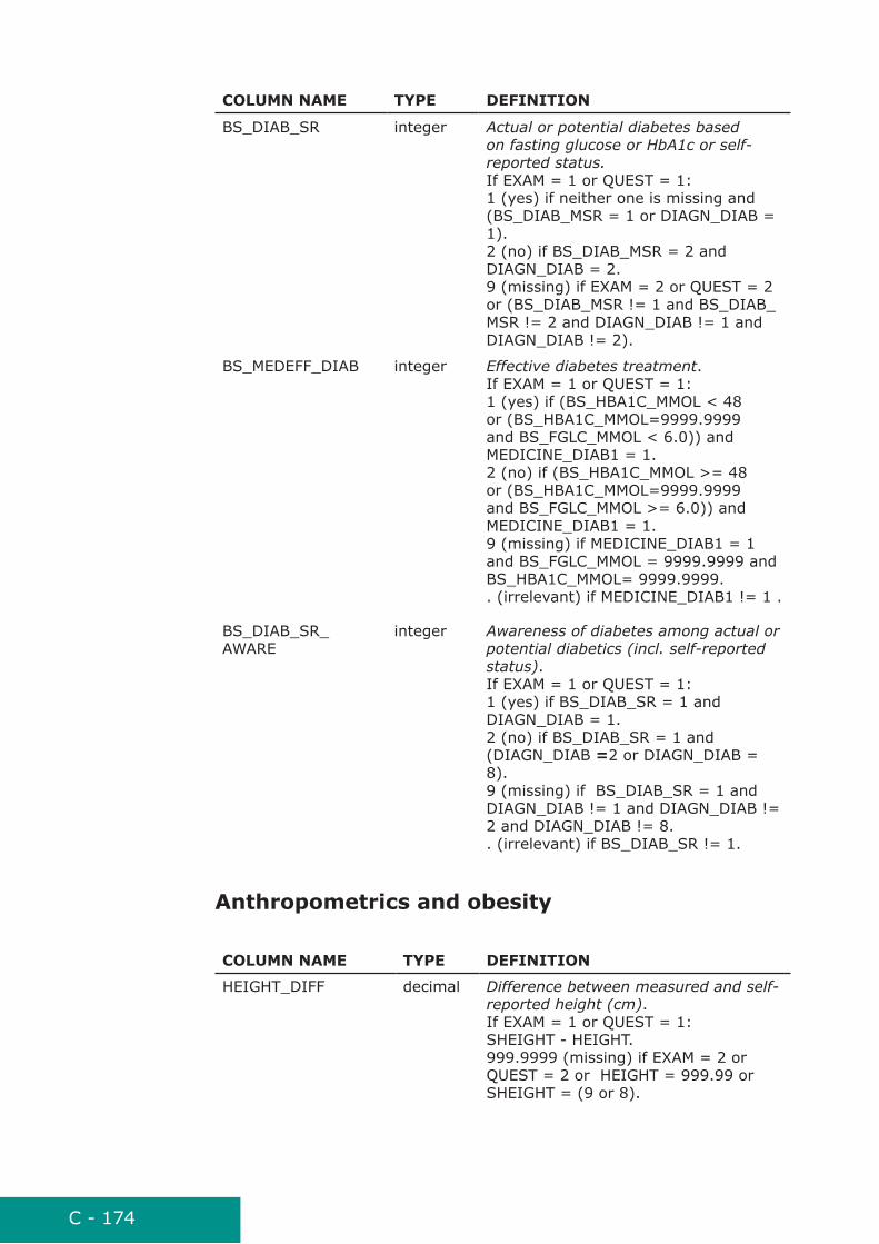
C - 174


BS_DIAB_SR integer Actual or potential diabetes based on fasting glucose or HbA1c or self-reported status. If EXAM = 1 or QUEST = 1: 1 (yes) if neither one is missing and (BS_DIAB_MSR = 1 or DIAGN_DIAB = 1). 2 (no) if BS_DIAB_MSR = 2 and DIAGN_DIAB = 2. 9 (missing) if EXAM = 2 or QUEST = 2 or (BS_DIAB_MSR != 1 and BS_DIAB_MSR != 2 and DIAGN_DIAB != 1 and DIAGN_DIAB != 2).

BS_MEDEFF_DIAB integer Effective diabetes treatment. If EXAM = 1 or QUEST = 1: 1 (yes) if (BS_HBA1C_MMOL < 48 or (BS_HBA1C_MMOL=9999.9999 and BS_FGLC_MMOL < 6.0)) and MEDICINE_DIAB1 = 1. 2 (no) if (BS_HBA1C_MMOL >= 48 or (BS_HBA1C_MMOL=9999.9999 and BS_FGLC_MMOL >= 6.0)) and MEDICINE_DIAB1 = 1. 9 (missing) if MEDICINE_DIAB1 = 1 and BS_FGLC_MMOL = 9999.9999 and BS_HBA1C_MMOL= 9999.9999. . (irrelevant) if MEDICINE_DIAB1 != 1 .

BS_DIAB_SR_AWARE

integer Awareness of diabetes among actual or potential diabetics (incl. self-reported status). If EXAM = 1 or QUEST = 1: 1 (yes) if BS_DIAB_SR = 1 and DIAGN_DIAB = 1. 2 (no) if BS_DIAB_SR = 1 and (DIAGN_DIAB =2 or DIAGN_DIAB = 8). 9 (missing) if BS_DIAB_SR = 1 and DIAGN_DIAB != 1 and DIAGN_DIAB != 2 and DIAGN_DIAB != 8. . (irrelevant) if BS_DIAB_SR != 1.

anthropometrics and obesity


HEIGHT_DIFF decimal Difference between measured and self-reported height (cm). If EXAM = 1 or QUEST = 1: SHEIGHT - HEIGHT. 999.9999 (missing) if EXAM = 2 or QUEST = 2 or HEIGHT = 999.99 or SHEIGHT = (9 or 8).

C - 175


WEIGHT_DIFF decimal Difference between measured and self-reported weight (kg). If EXAM = 1 or QUEST = 1: SWEIGHT - WEIGHT. 999.9999 (missing) if EXAM = 2 or QUEST = 2 or WEIGHT = 999.99 or SWEIGHT = (9 or 8).

BMI_DIFF decimal Difference between measured and self-reported BMI (kg/m2). If EXAM = 1 or QUEST = 1: BMI_SR - BMI if ELIG = 1 and EXAM = 1 and QUEST = 1. 999.9999 (missing) if BMI = 999.99 or BMI_SR = 999.99 and ELIG = 1 and EXAM = 1 and QUEST = 1. (empty value), if ELIG ≠ 1 or EXAM =2 or QUEST = 2.

BMI_CATEGORY integer BMI categories based on measured BMI. If EXAM = 1 or QUEST = 1: 1 (underweight) if BMI < 18.5. 2 (normal) if 18.5 <= BMI < 25. 3 (overweight) if 25 <= BMI < 30. 4 (grade 1 obese) if 30 <= BMI < 35. 5 (grade 2 overweight) if 35 <= BMI < 40. 6 (grade 3 overweight) if BMI >= 40. 9 (missing) if EXAM = 2 or BMI = 999.99.

BMI_OVERWEIGHT_SR integer Overweight based on self-reported BMI. If EXAM = 1 or QUEST = 1: 1 (yes) if BMI_SR >= 25. 2 (no) if BMI_SR < 25. 9 (missing) if QUEST = 2 or BMI_SR = 999.99.

BMI_OBESE_SR integer Obesity based on self-reported BMI. If EXAM = 1 or QUEST = 1: 1 (yes) if BMI_SR >= 30. 2 (no) if BMI_SSR < 30. 9 (missing) if QUEST = 2 or BMI_SR = 999.99.

BMI_CATEGORY_SR integer BMI categories based on self-reported BMI. If EXAM = 1 or QUEST = 1: 1 (underweight) if BMI_SR < 18.5. 2 (normal) if 18.5 <= BMI_SR < 25. 3 (overweight) if 25 <= BMI_SR < 30. 4 (grade 1 obese) if 30 <= BMI_SR < 35. 5 (grade 2 overweight) if 35 <= BMI_SR < 40. 6 (grade 3 overweight) if BMI_SR >= 40. 9 (missing) if QUEST = 2 or BMI_SR = 999.99.

C - 176

Smoking


SMOKEY integer Smoking years among all survey participants. If EXAM = 1 or QUEST = 1: SMOKE_YEARS if SMOKE = 1 or SMOKE_EVER = 1. 0, if (SMOKE = 2 or SMOKE = 3) and SMOKE_EVER = 2. 99 (missing) if QUEST = 2 or SMOKE_YEARS = 99 or (SMOKE != 1 and SMOKE != 2 and SMOKE != 3 and SMOKE_EVER != 1 and SMOKE_EVER != 2).

Eligibility and consent items


EXAM1 integer Participation in examination. EXAM if ELIG = 1. . (irrelvant) if ELIG != 1.

QUEST1 integer Participation in questionnaire. QUEST if ELIG = 1. . (irrelvant) if ELIG != 1.

REASON1 integer Reason for non-eligibility. REASON if ELIG = 2. . (irrelvant) if ELIG != 2.

EXAM_REF1 integer Refusal to participate to the examination. EXAM_REF if EXAM1 = 2. . (irrelvant) if EXAM1 != 2.

EXAM_NOAPP1 integer Interested but failed to make appointment for examination. EXAM_NOAPP if EXAM_REF1 != 2. . (irrelvant) if EXAM_REF1 = 2.

C - 177

Appendix 5c. Specification of indicatorsFor further information on indicators, see EHES Manual, Part C, Chap-ter 4.

Field name refer to the flag variable of the EHES database and variable names and values are defined in the EHES Manual, Part C, Chapter 2 for transferred data items and in the Appendix 5b. for the derived vari-ables.

Each indicator are calculated for men and women separately by 10-year age-groups and age-standardized for 25-64-year-olds. Other subgroups, e.g. socioeconomic status, can also be used. Indicators marked as green (v) are those that at least should be included in the basic report.

blood pressure indicators

FiElD naME DEFinition anD variablE naME anD valuES

n_nonmissing Number of individuals with non-missing value. Variables: BP_DIAST - Mean of diastolic blood pressure (mmHg). v BP_SYST - Mean of systolic blood pressure (mmHg). v BP_PULSE - Pulse rate (60 seconds).

mean Population mean. Variables: BP_DIAST - Mean of diastolic blood pressure (mmHg). v BP_SYST - Mean of systolic blood pressure (mmHg). v BP_PULSE - Pulse rate (60 seconds).

se Standard error of the mean. Variables: BP_DIAST - Mean of diastolic blood pressure (mmHg). v BP_SYST - Mean of systolic blood pressure (mmHg). v BP_PULSE - Pulse rate (60 seconds).

cil Lower limit of 95 % confidence interval of the mean. Variables: BP_DIAST - Mean of diastolic blood pressure (mmHg). v BP_SYST - Mean of systolic blood pressure (mmHg). v BP_PULSE - Pulse rate (60 seconds).

ciu Upper limit of 95 % confidence interval of the mean. Variables: BP_DIAST - Mean of diastolic blood pressure (mmHg). v BP_SYST - Mean of systolic blood pressure (mmHg). v BP_PULSE - Pulse rate (60 seconds).

Hypertension:

C - 178


n Number of individuals in each category. Variables: BP_AWARE - Awareness of hypertension among actual or potential hypertensives (140/90). v BP_HBP - Actual or potential hypertension (140/90). v BPM - When was blood pressure last measured by a health professional. 1 = Within the past 12 moths, 2 = 1-5 years ago, 3 = Never or more than 5 years ago. v BP_OPTIMAL - Optimal blood pressure among actual or potential hypertension (140/90). v DIAGN_HBP - High blood pressure (hypertension) diagnosed by medical doctor. v MEDICINE_HBP_POP - Medicines for high blood pressure during the past 2 two weeks among population. v MEDICINE_HBP_ILL - Medicines for high blood pressure during the past 2 two weeks among actual or potential hypertensives. v BP_CATEGORY - Categories of blood pressure: 1 = Optimal, 2 = Normal, 3 = High normal, 4 = Grade 1 hypertension, 5 = Grade 2 Hypertension, 6 = Grade 3 Hypertension. BP_EBP - Elevated blood pressure. BP_HSBP - Systolic hypertension. BP_MEDEFF_HBP - Effective antihypertensive drug treatment.

percent Proportion of each category among population with non-missing value. Variables: BP_AWARE - Awareness of hypertension among actual or potential hypertensives (140/90). v BP_HBP - Actual or potential hypertension (140/90). v BPM - When was blood pressure last measured by a health professional. 1 = Within the past 12 moths, 2 = 1-5 years ago, 3 = Never or more than 5 years ago. v BP_OPTIMAL - Optimal blood pressure among actual or potential hypertension (140/90). v DIAGN_HBP - High blood pressure (hypertension) diagnosed by medical doctor. v MEDICINE_HBP_POP - Medicines for high blood pressure during the past 2 two weeks among population. v MEDICINE_HBP_ILL - Medicines for high blood pressure during the past 2 two weeks among actual or potential hypertensives. v BP_CATEGORY - Categories of blood pressure: 1 = Optimal, 2 = Normal, 3 = High normal, 4 = Grade 1 hypertension, 5 = Grade 2 Hypertension, 6 = Grade 3 Hypertension. BP_EBP - Elevated blood pressure. BP_HSBP - Systolic hypertension. BP_MEDEFF_HBP - Effective antihypertensive drug treatment.

lipid indicators


n_nonmissing Number of individuals with non-missing value. Variables: BS_CHOL_MMOL - Serum total cholesterol in mmol/l. v BS_HDL_MMOL - Serum HDL cholesterol in mmol/l. v BS_NONHDL - Serum non-HDL cholesterol (mmol/l). v BS_CHOLHDL_RATIO - Ratio of serum total cholesterol and HDL cholesterol.

C - 179


mean Population mean. Variables: BS_CHOL_MMOL - Serum total cholesterol in mmol/l. v BS_HDL_MMOL - Serum HDL cholesterol in mmol/l. v BS_NONHDL - Serum non-HDL cholesterol (mmol/l). v BS_CHOLHDL_RATIO - Ratio of serum total cholesterol and HDL cholesterol.

se Standard error of the mean. Variables: BS_CHOL_MMOL - Serum total cholesterol in mmol/l. v BS_HDL_MMOL - Serum HDL cholesterol in mmol/l. v BS_NONHDL - Serum non-HDL cholesterol (mmol/l). v BS_CHOLHDL_RATIO - Ratio of serum total cholesterol and HDL cholesterol.

cil Lower limit of 95 % confidence interval of the mean. Variables: BS_CHOL_MMOL - Serum total cholesterol in mmol/l. v BS_HDL_MMOL - Serum HDL cholesterol in mmol/l. v BS_NONHDL - Serum non-HDL cholesterol (mmol/l). v BS_CHOLHDL_RATIO - Ratio of serum total cholesterol and HDL cholesterol.

ciu Upper limit of 95 % confidence interval of the mean. Variables: BS_CHOL_MMOL - Serum total cholesterol in mmol/l. v BS_HDL_MMOL - Serum HDL cholesterol in mmol/l. v BS_NONHDL - Serum non-HDL cholesterol (mmol/l). v BS_CHOLHDL_RATIO - Ratio of serum total cholesterol and HDL cholesterol.

C - 180


n Number of individuals in each category. Variables: BS_CHOL_AWARE - Awareness of elevated cholesterol among those with actual or potential elevated serum total cholesterol. 1 = Yes, 2 = No. v BS_CHOL_OPTIMAL - Optimal total cholesterol level (<5mmol/l) among those using lipid lowering drugs. 1 = Yes, 2 = No. v BS_HCHOL - Actual or potential elevated serum total cholesterol. 1 = Yes, 2 = No. v CHOLM - When was blood cholesterol last measured. 1 = Within the past 12 moths, 2 = 1-5 years ago, 3 = Never or more than 5 years ago. v DIAGN_CHOL - Elevated blood cholesterol diagnosed by medical doctor: 1 = Yes, 2 = No. v MEDICINE_CHOL_ILL - Medicines for lowering the blood cholesterol level during the past 2 two weeks among those with actual or potential elevated serum total cholesterol. 1 = Yes, 2 = No. v MEDICINE_CHOL_POP - Medicines for lowering the blood cholesterol level during the past 2 two weeks among population. 1 = Yes, 2 = No. v BS_CHOL_CATEGORY - Categories of serum total cholesterol. 1 = below 5 mmol/l, 2 = at least 5 and below 6, 3 = at least 6 and below 7, 4 = at least 7 and below 8, 5 = at least 8 mmol/l. BS_ECHOL - Elevated serum total cholesterol, cutpoint: 5 mmol/l. 1 = Yes, 2 = No. BS_ENONHDL - Elevated non-HDL cholesterol (>3.5mmol/l): 1 = Yes, 2 = No. BS_HNONHDL - Actual or potential elevated non-HDL cholesterol: 1 = Yes, 2 = No. BS_HRATIO - High serum total cholesterol to HDL cholesterol ratio (>5). 1 = Yes, 2 = No. BS_LHDL - Low serum HDL cholesterol <1mmol/l for men <1.2mmol/l for women): 1 = Yes, 2 = No. BS_MEDEFF_CHOL - Effective cholesterol treatment. 1 = Yes, 2 = No.

C - 181


percent Proportion of each category among population with non-missing value. Variables: BS_CHOL_AWARE - Awareness of elevated cholesterol among those with actual or potential elevated serum total cholesterol. 1 = Yes, 2 = No. v BS_CHOL_OPTIMAL - Optimal total cholesterol level (<5mmol/l) among those using lipid lowering drugs. 1 = Yes, 2 = No. v BS_HCHOL - Actual or potential elevated serum total cholesterol. 1 = Yes, 2 = No. v CHOLM - When was blood cholesterol last measured. 1 = Within the past 12 moths, 2 = 1-5 years ago, 3 = Never or more than 5 years ago. v DIAGN_CHOL - Elevated blood cholesterol diagnosed by medical doctor: 1 = Yes, 2 = No. v MEDICINE_CHOL_ILL - Medicines for lowering the blood cholesterol level during the past 2 two weeks among those with actual or potential elevated serum total cholesterol. 1 = Yes, 2 = No. v MEDICINE_CHOL_POP - Medicines for lowering the blood cholesterol level during the past 2 two weeks among population. 1 = Yes, 2 = No. v BS_CHOL_CATEGORY - Categories of serum total cholesterol. 1 = below 5 mmol/l, 2 = at least 5 and below 6, 3 = at least 6 and below 7, 4 = at least 7 and below 8, 5 = at least 8 mmol/l. BS_ECHOL - Elevated serum total cholesterol, cutpoint: 5 mmol/l. 1 = Yes, 2 = No. BS_ENONHDL - Elevated non-HDL cholesterol (>3.5mmol/l): 1 = Yes, 2 = No. BS_HNONHDL - Actual or potential elevated non-HDL cholesterol: 1 = Yes, 2 = No. BS_HRATIO - High serum total cholesterol to HDL cholesterol ratio (>5). 1 = Yes, 2 = No. BS_LHDL - Low serum HDL cholesterol (<1mmol/l for men <1.2mmol/l for women): 1 = Yes, 2 = No. BS_MEDEFF_CHOL - Effective cholesterol treatment. 1 = Yes, 2 = No.

Glucose and diabetes indicators


n_nonmissing Number of individuals with non-missing value. Variables: BS_FGLC_MMOL - Fasting plasma glucose in mmol/l. Relevant if BS_FAST = Yes. v BS_HBA1C_MMOL - Whole blood glycated haemoglobin concentration in mmol/mol. v

mean

Population mean. Variables: BS_FGLC_MMOL - Fasting plasma glucose in mmol/l. Relevant if BS_FAST = Yes. v BS_HBA1C_MMOL - Whole blood glycated haemoglobin concentration in mmol/mol. v

se Standard error of the mean. Variables: BS_FGLC_MMOL - Fasting plasma glucose in mmol/l. Relevant if BS_FAST = Yes. v BS_HBA1C_MMOL - Whole blood glycated haemoglobin concentration in mmol/mol. v

C - 182


cil Lower limit of 95 % confidence interval of the mean. Variables: BS_FGLC_MMOL - Fasting plasma glucose in mmol/l. Relevant if BS_FAST = Yes. v BS_HBA1C_MMOL - Whole blood glycated haemoglobin concentration in mmol/mol. v

ciu Upper limit of 95 % confidence interval of the mean. Variables: BS_FGLC_MMOL - Fasting plasma glucose in mmol/l. Relevant if BS_FAST = Yes. v BS_HBA1C_MMOL - Whole blood glycated haemoglobin concentration in mmol/mol. v

n Number of individuals in each category. Variables: BS_DIAB - Actual or potential diabetes based on fasting glucose or HbA1c or use of medication: 1 = Yes, 2 = No. v BS_DIAB_AWARE - Awareness of diabetes among actual or potential diabetics (incl. use of medication). 1 = Yes, 2 = No. v BS_GLC_OPTIMAL - Optimal fasting glucose or HbA1C level (<7mmol/l or <48mmol/mol) among those using diabetes medication. 1 = Yes, 2 = No. v DIAGN_DIAB - Diabetes diagnosed by medical doctor: 1 = Yes, 2 = No, 8 = Do not know. v GLCM - When was blood sugar (glucose) last measured. 1 = Within the past 12 moths, 2 = 1-5 years ago, 3 = Never or more than 5 years ago. v MEDICINE_DIAB_ILL - Medicines for diabetes during the past 2 two weeks among actual or potential diabetics. 1 = Yes, 2 = No. v MEDICINE_DIAB_POP - Medicines for diabetes during the past 2 two weeks among population. 1 = Yes, 2 = No. v BS_DIAB_MSR - Actual or potential diabetes based on fasting glucose or HbA1c: 1 = Yes, 2 = No. BS_DIAB_MSR2 - Actual or potential diabetes based on fasting glucose or HbA1c, lower limits. 1 = Yes, 2 = No. BS_DIAB_SR - Actual or potential diabetes based on fasting glucose or HbA1c or self-reported status: 1 = Yes, 2 = No. BS_GLYCEMIA - Provisional diagnosis of impaired fasting glucose (IFG): 1 = Yes, 2 = No. BS_DIAB_SR_AWARE - Awareness of diabetes among actual or potential diabetics (incl. self-reported status). 1 = Yes, 2 = No. BS_MEDEFF_DIAB - Effective diabetes treatment: 1 = Yes, 2 = No. BS_PROVDIAB_GLC - Provisional diagnosis of diabetes based on fasting plasma glucose: 1 = Yes, 2 = No. BS_PROVDIAB_HBA1C - Provisional diagnosis of diabetes based on HbA1c: 1 = Yes, 2 = No.

C - 183


percent Proportion of each category among population with non-missing value. Variables: BS_DIAB - Actual or potential diabetes based on fasting glucose or HbA1c or use of medication: 1 = Yes, 2 = No. v BS_DIAB_AWARE - Awareness of diabetes among actual or potential diabetics (incl. use of medication). 1 = Yes, 2 = No. v BS_GLC_OPTIMAL - Optimal fasting glucose or HbA1C level (<7mmol/l or <48mmol/mol) among those using diabetes medication. 1 = Yes, 2 = No. v DIAGN_DIAB - Diabetes diagnosed by medical doctor: 1 = Yes, 2 = No, 8 = Do not know. v GLCM - When was blood sugar (glucose) last measured. 1 = Within the past 12 moths, 2 = 1-5 years ago, 3 = Never or more than 5 years ago. v MEDICINE_DIAB_ILL - Medicines for diabetes during the past 2 two weeks among actual or potential diabetics. 1 = Yes, 2 = No. v MEDICINE_DIAB_POP - Medicines for diabetes during the past 2 two weeks among population. 1 = Yes, 2 = No. v BS_DIAB_MSR - Actual or potential diabetes based on fasting glucose or HbA1c: 1 = Yes, 2 = No. BS_DIAB_MSR2 - Actual or potential diabetes based on fasting glucose or HbA1c, lower limits. 1 = Yes, 2 = No. BS_DIAB_SR - Actual or potential diabetes based on fasting glucose or HbA1c or self-reported status: 1 = Yes, 2 = No. BS_GLYCEMIA - Provisional diagnosis of impaired fasting glucose (IFG): 1 = Yes, 2 = No. BS_DIAB_SR_AWARE - Awareness of diabetes among actual or potential diabetics (incl. self-reported status). 1 = Yes, 2 = No. BS_MEDEFF_DIAB - Effective diabetes treatment: 1 = Yes, 2 = No. BS_PROVDIAB_GLC - Provisional diagnosis of diabetes based on fasting plasma glucose: 1 = Yes, 2 = No. BS_PROVDIAB_HBA1C - Provisional diagnosis of diabetes based on HbA1c: 1 = Yes, 2 = No.

anthropometric and obesity indicators


n_nonmissig Number of individuals with non-missing value. Variables: BMI - Body mass index (kg/m2) based on measured height and weight. v BMI_SR - Body mass index (kg/m2) based on self-reported height and weight. v WAIST - Waist circumference in cm. v BMI_DIFF - Difference between measured and self-reported BMI in kg/m2 (self-reported - measured). HEIGHT - Height in cm. HEIGHT_DIFF - Difference between measured and self-reported height in cm (self-reported - measured). SHEIGHT - Self-reported height (cm). SWEIGHT - Self-reported weight (kg). WEIGHT - Weight in kg. WEIGHT_DIFF - Difference between measured and self-reported weight in kg (self-reported - measured).

C - 184


mean Population mean. Variables: BMI - Body mass index (kg/m2) based on measured height and weight. v BMI_SR - Body mass index (kg/m2) based on self-reported height and weight. v WAIST - Waist circumference in cm. v BMI_DIFF - Difference between measured and self-reported BMI in kg/m2 (self-reported - measured). HEIGHT - Height in cm. HEIGHT_DIFF - Difference between measured and self-reported height in cm (self-reported - measured). SHEIGHT - Self-reported height (cm). SWEIGHT - Self-reported weight (kg). WEIGHT - Weight in kg. WEIGHT_DIFF - Difference between measured and self-reported weight in kg (self-reported - measured).

se Standard error of the mean. Variables: BMI - Body mass index (kg/m2) based on measured height and weight. v BMI_SR - Body mass index (kg/m2) based on self-reported height and weight. v WAIST - Waist circumference in cm. v BMI_DIFF - Difference between measured and self-reported BMI in kg/m2 (self-reported - measured). HEIGHT - Height in cm. HEIGHT_DIFF - Difference between measured and self-reported height in cm (self-reported - measured). SHEIGHT - Self-reported height (cm). SWEIGHT - Self-reported weight (kg). WEIGHT - Weight in kg. WEIGHT_DIFF - Difference between measured and self-reported weight in kg (self-reported - measured).

cil Lower limit of 95 % confidence interval of the mean. Variables: BMI - Body mass index (kg/m2) based on measured height and weight. v BMI_SR - Body mass index (kg/m2) based on self-reported height and weight. v WAIST - Waist circumference in cm. v BMI_DIFF - Difference between measured and self-reported BMI in kg/m2 (self-reported - measured). HEIGHT - Height in cm. HEIGHT_DIFF - Difference between measured and self-reported height in cm (self-reported - measured). SHEIGHT - Self-reported height (cm). SWEIGHT - Self-reported weight (kg). WEIGHT - Weight in kg. WEIGHT_DIFF - Difference between measured and self-reported weight in kg (self-reported - measured).

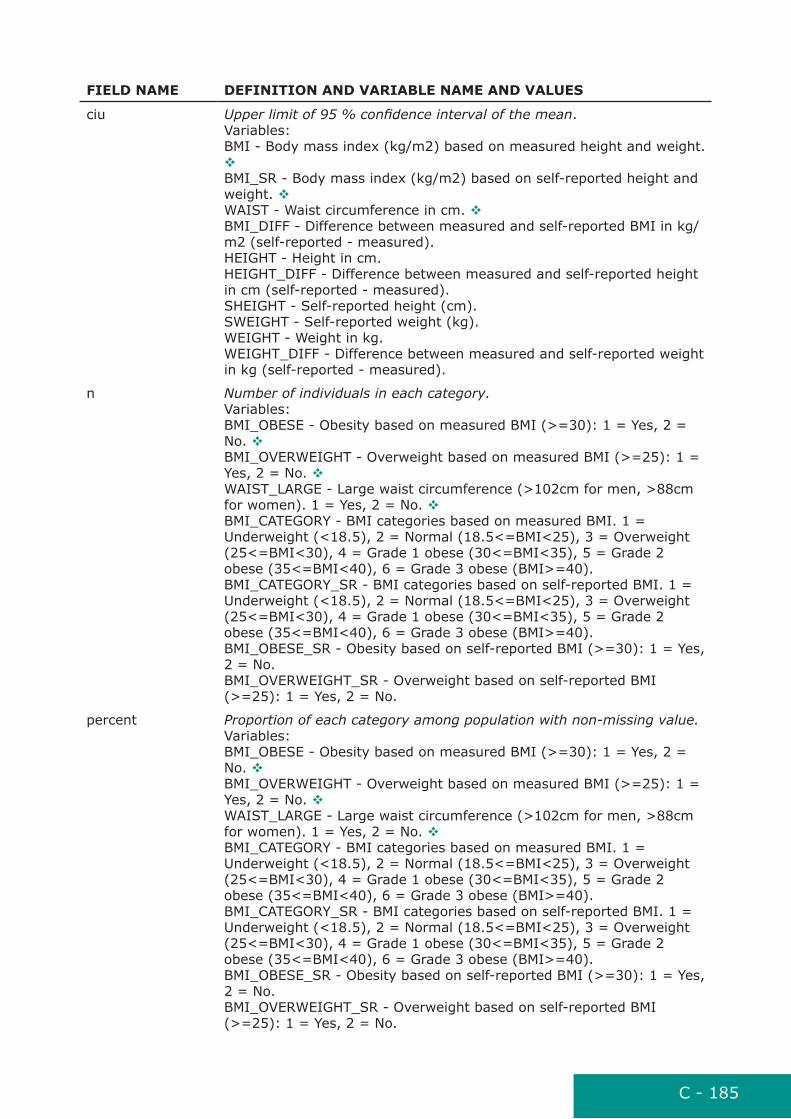
C - 185


ciu Upper limit of 95 % confidence interval of the mean. Variables: BMI - Body mass index (kg/m2) based on measured height and weight. v BMI_SR - Body mass index (kg/m2) based on self-reported height and weight. v WAIST - Waist circumference in cm. v BMI_DIFF - Difference between measured and self-reported BMI in kg/m2 (self-reported - measured). HEIGHT - Height in cm. HEIGHT_DIFF - Difference between measured and self-reported height in cm (self-reported - measured). SHEIGHT - Self-reported height (cm). SWEIGHT - Self-reported weight (kg). WEIGHT - Weight in kg. WEIGHT_DIFF - Difference between measured and self-reported weight in kg (self-reported - measured).

n Number of individuals in each category. Variables: BMI_OBESE - Obesity based on measured BMI (>=30): 1 = Yes, 2 = No. v BMI_OVERWEIGHT - Overweight based on measured BMI (>=25): 1 = Yes, 2 = No. v WAIST_LARGE - Large waist circumference (>102cm for men, >88cm for women). 1 = Yes, 2 = No. v BMI_CATEGORY - BMI categories based on measured BMI. 1 = Underweight (<18.5), 2 = Normal (18.5<=BMI<25), 3 = Overweight (25<=BMI<30), 4 = Grade 1 obese (30<=BMI<35), 5 = Grade 2 obese (35<=BMI<40), 6 = Grade 3 obese (BMI>=40). BMI_CATEGORY_SR - BMI categories based on self-reported BMI. 1 = Underweight (<18.5), 2 = Normal (18.5<=BMI<25), 3 = Overweight (25<=BMI<30), 4 = Grade 1 obese (30<=BMI<35), 5 = Grade 2 obese (35<=BMI<40), 6 = Grade 3 obese (BMI>=40). BMI_OBESE_SR - Obesity based on self-reported BMI (>=30): 1 = Yes, 2 = No. BMI_OVERWEIGHT_SR - Overweight based on self-reported BMI (>=25): 1 = Yes, 2 = No.

percent Proportion of each category among population with non-missing value. Variables: BMI_OBESE - Obesity based on measured BMI (>=30): 1 = Yes, 2 = No. v BMI_OVERWEIGHT - Overweight based on measured BMI (>=25): 1 = Yes, 2 = No. v WAIST_LARGE - Large waist circumference (>102cm for men, >88cm for women). 1 = Yes, 2 = No. v BMI_CATEGORY - BMI categories based on measured BMI. 1 = Underweight (<18.5), 2 = Normal (18.5<=BMI<25), 3 = Overweight (25<=BMI<30), 4 = Grade 1 obese (30<=BMI<35), 5 = Grade 2 obese (35<=BMI<40), 6 = Grade 3 obese (BMI>=40). BMI_CATEGORY_SR - BMI categories based on self-reported BMI. 1 = Underweight (<18.5), 2 = Normal (18.5<=BMI<25), 3 = Overweight (25<=BMI<30), 4 = Grade 1 obese (30<=BMI<35), 5 = Grade 2 obese (35<=BMI<40), 6 = Grade 3 obese (BMI>=40). BMI_OBESE_SR - Obesity based on self-reported BMI (>=30): 1 = Yes, 2 = No. BMI_OVERWEIGHT_SR - Overweight based on self-reported BMI (>=25): 1 = Yes, 2 = No.

C - 186

Self-perceived health and chronic disease indicators


n Number of individuals in each category. Variables: HEALTH_GOOD - Self-perceived health reported to be good or very good. 1 = Yes, 2 = No. v LIMITED_YES - Person reported that she has limitations in daily activities due to health problems. 1 = Yes, 2 = No. v HEALTH_PROBLEM - Longstanding illness or health problem. 1 = Yes, 2 = No. DIAGN_MI - Myocardial infarction diagnosed by medical doctor: 1 = Yes, 2 = No. DIAGN_STROKE - Stroke (cerebral haemorrhage, cerebral thrombosis) diagnosed by medical doctor: 1 = Yes, 2 = No. DIAGN_CHD - Coronary heart disease (angina pectoris) diagnosed by medical doctor: 1 = Yes, 2 = No.

percent Proportion of each category among population with non-missing value. Variables: HEALTH_GOOD - Self-perceived health reported to be good or very good. 1 = Yes, 2 = No. v LIMITED_YES - Person reported that she has limitations in daily activities due to health problems. 1 = Yes, 2 = No. v HEALTH_PROBLEM - Longstanding illness or health problem. 1 = Yes, 2 = No.DIAGN_MI - Myocardial infarction diagnosed by medical doctor: 1 = Yes, 2 = No. DIAGN_STROKE - Stroke (cerebral haemorrhage, cerebral thrombosis) diagnosed by medical doctor: 1 = Yes, 2 = No. DIAGN_CHD - Coronary heart disease (angina pectoris) diagnosed by medical doctor: 1 = Yes, 2 = No.

Smoking indicators


n_nonmissing Number of individuals with non-missing value. Variables: SMOKEY - Smoking years in whole population. SMOKE_YEARS - Daily smoking years.

mean Population mean. Variables: SMOKEY - Smoking years in whole population. SMOKE_YEARS - Daily smoking years.

se Standard error of the mean. Variables: SMOKEY - Smoking years in whole population. SMOKE_YEARS - Daily smoking years.

cil Lower limit of 95 % confidence interval of the mean. Variables: SMOKEY - Smoking years in whole population. SMOKE_YEARS - Daily smoking years.

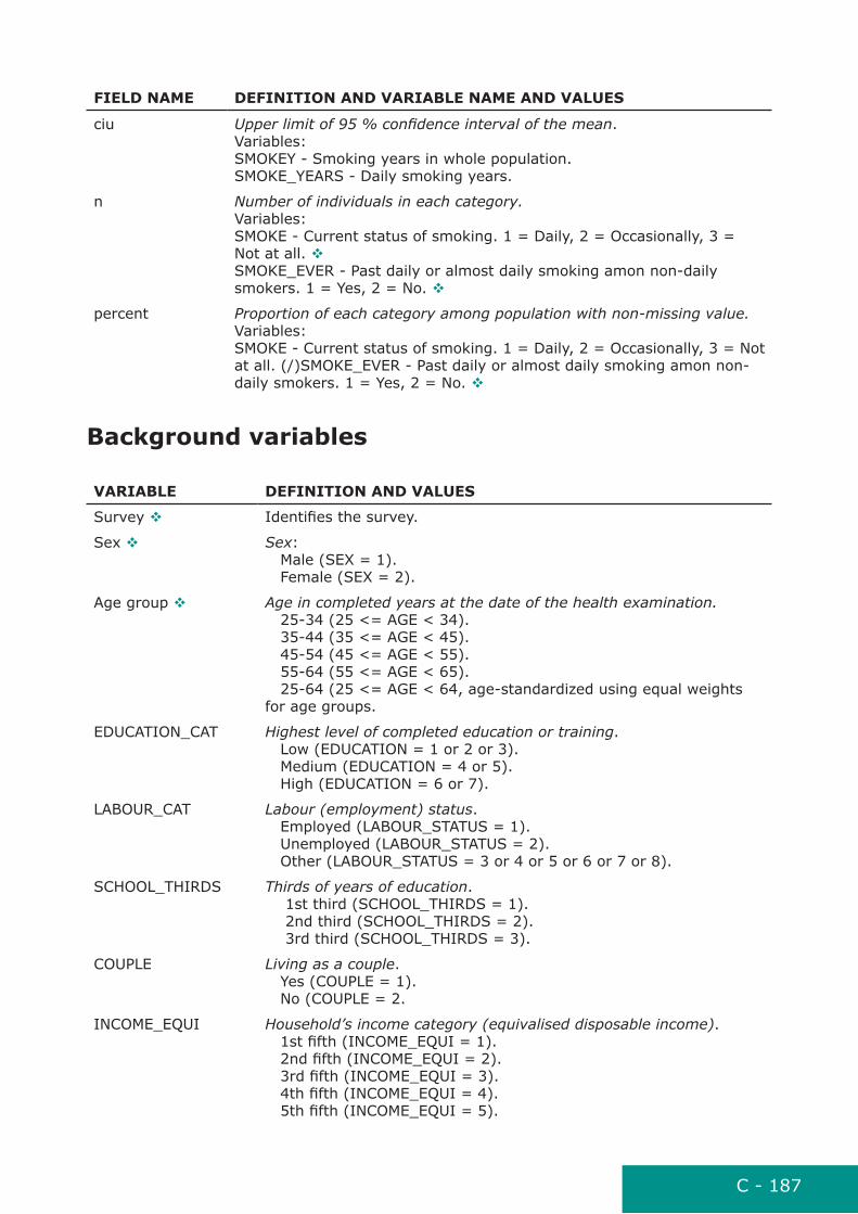
C - 187


ciu Upper limit of 95 % confidence interval of the mean. Variables: SMOKEY - Smoking years in whole population. SMOKE_YEARS - Daily smoking years.

n Number of individuals in each category. Variables: SMOKE - Current status of smoking. 1 = Daily, 2 = Occasionally, 3 = Not at all. v SMOKE_EVER - Past daily or almost daily smoking amon non-daily smokers. 1 = Yes, 2 = No. v

percent Proportion of each category among population with non-missing value. Variables: SMOKE - Current status of smoking. 1 = Daily, 2 = Occasionally, 3 = Not at all. (/)SMOKE_EVER - Past daily or almost daily smoking amon non-daily smokers. 1 = Yes, 2 = No. v

background variables

variablE DEFinition anD valuES

Survey v Identifies the survey.

Sex v Sex: Male (SEX = 1). Female (SEX = 2).

Age group v Age in completed years at the date of the health examination. 25-34 (25 <= AGE < 34). 35-44 (35 <= AGE < 45). 45-54 (45 <= AGE < 55). 55-64 (55 <= AGE < 65). 25-64 (25 <= AGE < 64, age-standardized using equal weights for age groups.

EDUCATION_CAT Highest level of completed education or training. Low (EDUCATION = 1 or 2 or 3). Medium (EDUCATION = 4 or 5). High (EDUCATION = 6 or 7).

LABOUR_CAT Labour (employment) status. Employed (LABOUR_STATUS = 1). Unemployed (LABOUR_STATUS = 2). Other (LABOUR_STATUS = 3 or 4 or 5 or 6 or 7 or 8).

SCHOOL_THIRDS Thirds of years of education. 1st third (SCHOOL_THIRDS = 1). 2nd third (SCHOOL_THIRDS = 2). 3rd third (SCHOOL_THIRDS = 3).

COUPLE Living as a couple. Yes (COUPLE = 1). No (COUPLE = 2.

INCOME_EQUI Household’s income category (equivalised disposable income). 1st fifth (INCOME_EQUI = 1). 2nd fifth (INCOME_EQUI = 2). 3rd fifth (INCOME_EQUI = 3). 4th fifth (INCOME_EQUI = 4). 5th fifth (INCOME_EQUI = 5).

C - 188

appendix 5d. Program codes for basic reportingFollowing R scripts are used in EHES basic reporting.

Database connection is established using R package RODBC (Brian Ripley and from 1999 to Oct 2002 Michael Lapsley (2012). RODBC: ODBC Database Access. R pack-age version 1.3-5. http://CRAN.R-project.org/package=RODBC) and SQL (Structured Query Language) is used to import and export data from EHES database.
















General functions

select_obs - to select relevant individuals for variable varname in the data using filters defined in variables

select_obs <- function(data, variables, varname) { ### data = dataset where to select observations, variables = definition table for variables, varname = name of the variable irr = variables$IRRELEVANT[variables$VARNAME==varname] ## filtering individuals using participation indicator variables EXAM and QUEST if (variables$EXAM[variables$VARNAME==varname]==”1” & variables$QUEST[variables$VARNAME==varname]==”1”) { selected <- data[data$EXAM == ”1” & data$QUEST == ”1” & !(data[,

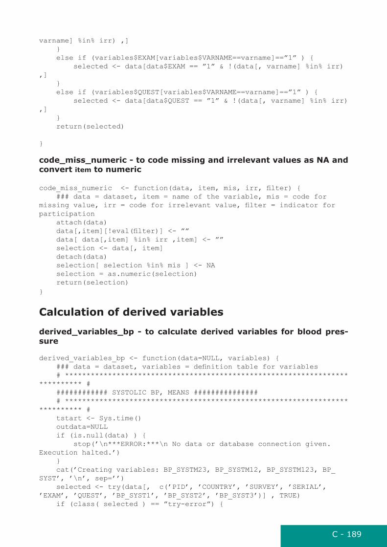
C - 189

varname] %in% irr) ,] } else if (variables$EXAM[variables$VARNAME==varname]==”1” ) { selected <- data[data$EXAM == ”1” & !(data[, varname] %in% irr) ,] } else if (variables$QUEST[variables$VARNAME==varname]==”1” ) { selected <- data[data$QUEST == ”1” & !(data[, varname] %in% irr) ,] } return(selected)

}

code_miss_numeric - to code missing and irrelevant values as na and convert item to numeric

code_miss_numeric <- function(data, item, mis, irr, filter) { ### data = dataset, item = name of the variable, mis = code for missing value, irr = code for irrelevant value, filter = indicator for participation attach(data) data[,item][!eval(filter)] <- ”” data[ data[,item] %in% irr ,item] <- ”” selection <- data[, item] detach(data) selection[ selection %in% mis ] <- NA selection = as.numeric(selection) return(selection)}

Calculation of derived variables

derived_variables_bp - to calculate derived variables for blood pres-sure

derived_variables_bp <- function(data=NULL, variables) { ### data = dataset, variables = definition table for variables # **************************************************************************** # ############ SYSTOLIC BP, MEANS ############### # **************************************************************************** # tstart <- Sys.time() outdata=NULL if (is.null(data) ) { stop(’\n***ERROR:***\n No data or database connection given. Execution halted.’) } cat(’Creating variables: BP_SYSTM23, BP_SYSTM12, BP_SYSTM123, BP_SYST’, ’\n’, sep=’’) selected <- try(data[, c(’PID’, ’COUNTRY’, ’SURVEY’, ’SERIAL’, ’EXAM’, ’QUEST’, ’BP_SYST1’, ’BP_SYST2’, ’BP_SYST3’)] , TRUE) if (class( selected ) == ”try-error”) {

C - 190

stop(paste(’Selected variables not found from dataset ’, data, ’\n’, sep=””)) } # to filter the participants filters <- expression(EXAM == ’1’ | QUEST == ’1’) attach(selected) selected = selected[eval(filters),] detach(selected) irr <- ”” mis = variables$MISSING[variables$VARNAME == ”BP_SYST1”] ## coding missing values and convert to numeric selected$BP_SYST1 = code_miss_numeric(selected, ’BP_SYST1’, mis=mis, irr=irr, filter=filters) selected$BP_SYST2 = code_miss_numeric(selected, ’BP_SYST2’, mis=mis, irr=irr, filter=filters) selected$BP_SYST3 = code_miss_numeric(selected, ’BP_SYST3’, mis=mis, irr=irr, filter=filters) ### BP_SYSTM23, BP_SYSTM12, BP_SYSTM123 mis = variables$MISSING[variables$VARNAME == ”BP_SYST”] irr = variables$IRRELEVANT[variables$VARNAME == ”BP_SYST”] selected$BP_SYSTM23 <- format(round(rowMeans( selected[, c(’BP_SYST2’, ’BP_SYST3’)]), 2), nsmall=2, trim=T) attach(selected) selected$BP_SYSTM23[!eval(filters)] <- irr selected$BP_SYSTM23[eval(filters) & selected$BP_SYSTM23 == ”NA”] <- mis detach(selected) selected$BP_SYSTM12 <- format(round(rowMeans( selected[, c(’BP_SYST1’, ’BP_SYST2’)]), 2), nsmall=2, trim=T) attach(selected) selected$BP_SYSTM12[!eval(filters)] <- irr selected$BP_SYSTM12[eval(filters) & selected$BP_SYSTM12 == ”NA”] <- mis detach(selected) selected$BP_SYSTM123 <- format(round(rowMeans( selected[, c(’BP_SYST1’, ’BP_SYST2’, ’BP_SYST3’)]), 2), nsmall=2, trim=T) attach(selected) selected$BP_SYSTM123[!eval(filters)] <- irr selected$BP_SYSTM123[eval(filters) & selected$BP_SYSTM123 == ”NA”] <- mis detach(selected) #### BP_SYST selected$BP_SYST <- mean_variables_bp(selected, item=c(’BP_SYST’) , variables=variables) attach(selected) selected$BP_SYST[!eval(filters)] <- irr selected$BP_SYST[eval(filters) & selected$BP_SYST == ”NA”] <- mis detach(selected) selected <- try(selected[, c(’PID’, ’COUNTRY’, ’SURVEY’, ’SERIAL’, ’EXAM’, ’QUEST’, ’BP_SYSTM23’, ’BP_SYSTM12’, ’BP_SYSTM123’, ’BP_SYST’)], TRUE) if (class( selected ) == ”try-error”) { stop(paste(’Selected variables not found from dataset.’, ’\n’, sep=””)) }

C - 191

if (!is.null(outdata) ) { outdata <- merge(outdata, selected, all=T) } if (is.null(outdata)) { outdata <- selected } selected = NULL filters = NULL

# **************************************************************************** # ############ DIASTOLIC BP, MEANS ############### # **************************************************************************** # cat(’Creating variables: BP_DIASTM23, BP_DIASTM12, BP_DIASTM123, BP_DIAST’, ’\n’, sep=’’) selected <- try(data[ , c(’PID’, ’COUNTRY’, ’SURVEY’, ’SERIAL’, ’EXAM’, ’QUEST’, ’BP_DIAST1’, ’BP_DIAST2’, ’BP_DIAST3’)] , TRUE) if (class( selected ) == ”try-error”) { stop(paste(’Selected variables not found from dataset\n’, sep=””)) } ### filtering all derived variables as EXAM=1 or QUEST=1 filters <- expression(EXAM == ’1’ | QUEST == ’1’) attach(selected) selected = selected[eval(filters),] detach(selected) irr <- variables$IRRELEVANT[variables$VARNAME == ”BP_DIAST1”] mis = variables$MISSING[variables$VARNAME == ”BP_DIAST1”] ## coding missing values and convert to numeric selected$BP_DIAST1 = code_miss_numeric(selected, ’BP_DIAST1’, mis, irr, filter=filters ) selected$BP_DIAST2 = code_miss_numeric(selected, ’BP_DIAST2’, mis, irr, filter=filters) selected$BP_DIAST3 = code_miss_numeric(selected, ’BP_DIAST3’, mis, irr, filter=filters) ### BP_DIASTM23, BP_DIASTM12, BP_DIASTM123 mis = variables$MISSING[variables$VARNAME == ”BP_DIASTM23”] irr = variables$IRRELEVANT[variables$VARNAME == ”BP_DIASTM23”] selected$BP_DIASTM23 <- format(round(rowMeans( selected[, c(’BP_DIAST2’, ’BP_DIAST3’)]), 2), nsmall=2, trim=T) attach(selected) selected$BP_DIASTM23[!eval(filters)] <- irr selected$BP_DIASTM23[eval(filters) & selected$BP_DIASTM23 == ”NA”] <- mis detach(selected) attach(selected) selected$BP_DIASTM12 <- format(round(rowMeans( selected[, c(’BP_DIAST1’, ’BP_DIAST2’)]), 2), nsmall=2, trim=T) selected$BP_DIASTM12[!eval(filters)] <- irr selected$BP_DIASTM12[eval(filters) & selected$BP_DIASTM12 == ”NA”] <- mis detach(selected) attach(selected) selected$BP_DIASTM123 <- format(round(rowMeans( selected[, c(’BP_

C - 192

DIAST1’, ’BP_DIAST2’, ’BP_DIAST3’)]), 2), nsmall=2, trim=T) selected$BP_DIASTM123[!eval(filters)] <- irr selected$BP_DIASTM123[eval(filters) & selected$BP_DIASTM123 == ”NA”] <- mis detach(selected) #### BP_DIAST selected$BP_DIAST <- mean_variables_bp(selected, item=c(’BP_DIAST’), variables=variables ) attach(selected) selected$BP_DIAST[!eval(filters)] <- irr selected$BP_DIAST[eval(filters) & selected$BP_DIAST == ”NA”] <- mis detach(selected) selected <- try(selected[, c(’PID’, ’COUNTRY’, ’SURVEY’, ’SERIAL’, ’EXAM’, ’QUEST’, ’BP_DIASTM23’, ’BP_DIASTM12’, ’BP_DIASTM123’, ’BP_DIAST’)], TRUE) if (class( selected ) == ”try-error”) { stop(paste(’Selected variables not found from dataset.’, ’\n’, sep=””)) } if (!is.null(outdata) ) { outdata <- merge(outdata, selected, all=T) } if (is.null(outdata)) { outdata <- selected }

# **************************************************************************** # ############ HYPERTENSION ############### # **************************************************************************** # cat(’Creating variables: MEDICINE_HBP1, BP_HBP, BP_HBP2, BP_HSBP, BP_EBP, BP_CATEGORY, BP_MEDEFF_HBP, BP_AWARE, BP_AWARE2\n, MEDICINE_HBP_POP, MEDICINE_HBP_ILL, BP_OPTIMAL’, ’\n’, sep=’’) selected1 <- try(data[ , c(’PID’, ’COUNTRY’, ’SURVEY’, ’SERIAL’, ’EXAM’, ’QUEST’ , ’MEDICINE’, ’MEDICINE_HBP’, ’DIAGN_HBP’)] , TRUE) if (class( selected1 ) == ”try-error”) { stop(paste(’Selected variables not found from dataset\n’, sep=””)) } selected <- merge(selected1, outdata , all=T) ### filtering all derived variables as EXAM=1 or QUEST=1 filters <- expression(EXAM == ’1’ | QUEST == ’1’) attach(selected) selected = selected[eval(filters),] detach(selected) irr <- variables$IRRELEVANT[variables$VARNAME == ”BP_SYST”] mis = variables$MISSING[variables$VARNAME == ”BP_SYST”] selected$BP_SYST = code_miss_numeric(selected, ’BP_SYST’, mis, irr, filter=filters) selected$BP_DIAST = code_miss_numeric(selected, ’BP_DIAST’, mis, irr, filter=filters)

# **************************************************************************** #

C - 193

############ TREATMENT FOR HYPERTENSION ############### # **************************************************************************** # ### Medicines for high blood pressure MEDICINE_HBP1 mis = variables$MISSING[variables$VARNAME == ”MEDICINE_HBP1”] attach(selected) selected$MEDICINE_HBP1[!eval(filters)] <- irr selected$MEDICINE_HBP1[eval(filters) & MEDICINE != ”1” ] <- ”.” selected$MEDICINE_HBP1[eval(filters) & MEDICINE == ”1” & MEDICINE_HBP == ”1” ] <- ”1” selected$MEDICINE_HBP1[eval(filters) & ((MEDICINE == ”1” & MEDICINE_HBP == ”2”) ) ] <- ”2” selected$MEDICINE_HBP1[eval(filters) & (MEDICINE == ”1” & MEDICINE_HBP != ”1” & MEDICINE_HBP != ”2”) ] <- mis detach(selected) #### Actual or potential hypertension BP_HBP mis = variables$MISSING[variables$VARNAME == ”BP_HBP”] attach(selected) selected$BP_HBP[!eval(filters)] <- irr selected$BP_HBP[eval(filters) & ((BP_SYST >= 140 | BP_DIAST >= 90 | MEDICINE_HBP1 == ”1”) & MEDICINE != ”9” & MEDICINE_HBP1 != ”9” & !is.na(BP_SYST) & !is.na(BP_DIAST)) ] <- ”1” selected$BP_HBP[eval(filters) & (BP_SYST < 140 & BP_DIAST < 90 ) & (MEDICINE_HBP1 != ”1” & MEDICINE_HBP1 != ”9”) ] <- ”2” selected$BP_HBP[eval(filters) & (is.na(BP_SYST) | is.na(BP_DIAST) ) | (MEDICINE_HBP1 == ”9” | MEDICINE == ”9”) ] <- mis detach(selected) #### Actual or potential hypertension BP_HBP2, higher limits mis = variables$MISSING[variables$VARNAME == ”BP_HBP2”] attach(selected) selected$BP_HBP2[!eval(filters)] <- irr selected$BP_HBP2[eval(filters) & ((BP_SYST >= 160 | BP_DIAST >= 100 | MEDICINE_HBP1 == ”1”) & !is.na(BP_SYST) & !is.na(BP_DIAST) & MEDICINE_HBP1 != ”9” & MEDICINE != ”9”) ] <- ”1” selected$BP_HBP2[eval(filters) & ((BP_SYST < 160 & BP_DIAST < 100 ) & MEDICINE_HBP1 != ”1” & MEDICINE_HBP1 != ”9”) ] <- ”2” selected$BP_HBP2[eval(filters) & (is.na(BP_SYST) | is.na(BP_DIAST) ) | MEDICINE_HBP1 == ”9” | MEDICINE == ”9”] <- mis detach(selected) #### Effective antihypertensive drug treatment BP_MEDEFF_HBP mis = variables$MISSING[variables$VARNAME == ”BP_MEDEFF_HBP”] attach(selected) selected$BP_MEDEFF_HBP[!eval(filters)] <- irr selected$BP_MEDEFF_HBP[eval(filters) & MEDICINE_HBP1 != ”1” ] <- ”.” selected$BP_MEDEFF_HBP[eval(filters) & BP_SYST < 140 & BP_DIAST < 90 & MEDICINE_HBP1 == ”1” ] <- ”1” selected$BP_MEDEFF_HBP[eval(filters) & ((BP_SYST >= 140 | BP_DIAST >= 90 ) & MEDICINE_HBP1 == ”1”) ] <- ”2” selected$BP_MEDEFF_HBP[eval(filters) & (is.na(BP_SYST) | is.na(BP_DIAST)) & MEDICINE_HBP1 == ”1”] <- mis ### Medicines for high blood pressure among population MEDICINE_HBP_POP mis = variables$MISSING[variables$VARNAME == ”MEDICINE_HBP_POP”] selected$MEDICINE_HBP_POP[!eval(filters)] <- irr selected$MEDICINE_HBP_POP[eval(filters) & MEDICINE_HBP1 == ”1” ] <-

C - 194

”1” selected$MEDICINE_HBP_POP[eval(filters) & (MEDICINE_HBP1 == ”2” | MEDICINE == ”2”) ] <- ”2” selected$MEDICINE_HBP_POP[eval(filters) & ((MEDICINE == ”1” & MEDICINE_HBP1 == ”9”) | (MEDICINE != ”1” & MEDICINE != ”2” ) ) ] <- mis ### Medicines for high blood pressure among actual or potential MEDICINE_HBP_ILL mis = variables$MISSING[variables$VARNAME == ”MEDICINE_HBP_ILL”] selected$MEDICINE_HBP_ILL[!eval(filters)] <- irr selected$MEDICINE_HBP_ILL[eval(filters) & BP_HBP != ”1” ] <- ”.” selected$MEDICINE_HBP_ILL[eval(filters) & BP_HBP == ”1” & MEDICINE_HBP1 == ”1” ] <- ”1” selected$MEDICINE_HBP_ILL[eval(filters) & ((BP_HBP == ”1” & MEDICINE_HBP1 == ”2”) | (BP_HBP == ”1” & MEDICINE == ”2”)) ] <- ”2” selected$MEDICINE_HBP_ILL[eval(filters) & (BP_HBP == ”1” & MEDICINE_HBP1 == ”9”) | (BP_HBP == ”1” & MEDICINE == ”9”) ] <- mis detach(selected) attach(selected) #### Systolic hypertension BP_HSBP mis = variables$MISSING[variables$VARNAME == ”BP_HSBP”] selected$BP_HSBP[!eval(filters)] <- irr selected$BP_HSBP[eval(filters) & BP_SYST >= 140 ] <- ”1” selected$BP_HSBP[eval(filters) & BP_SYST < 140 ] <- ”2” selected$BP_HSBP[eval(filters) & is.na(BP_SYST) ] <- mis #### Elevated blood pressure BP_EBP mis = variables$MISSING[variables$VARNAME == ”BP_EBP”] selected$BP_EBP[!eval(filters)] <- irr selected$BP_EBP[eval(filters) & (BP_SYST >= 140 | BP_DIAST >= 90) ] <- ”1” selected$BP_EBP[eval(filters) & BP_SYST < 140 & BP_DIAST < 90 ] <- ”2” selected$BP_EBP[eval(filters) & (is.na(BP_SYST) | is.na(BP_DIAST)) ] <- mis detach(selected) attach(selected) ### Optimal blood pressure among those using anti-hypertensive drugs BP_OPTIMAL mis = variables$MISSING[variables$VARNAME == ”BP_OPTIMAL”] selected$BP_OPTIMAL[!eval(filters)] <- irr selected$BP_OPTIMAL[eval(filters) & MEDICINE_HBP1 != ”1” ] <- ”.” selected$BP_OPTIMAL[eval(filters) & MEDICINE_HBP1 == ”1” & BP_EBP == ”2” ] <- ”1” selected$BP_OPTIMAL[eval(filters) & MEDICINE_HBP1 == ”1” & BP_EBP == ”1” ] <- ”2” selected$BP_OPTIMAL[eval(filters) & MEDICINE_HBP1 == ”1” & BP_EBP != ”1” & BP_EBP != ”2” ] <- mis #### Categories of blood pressure BP_CATEGORY mis = variables$MISSING[variables$VARNAME == ”BP_CATEGORY”] selected$BP_CATEGORY[!eval(filters)] <- irr selected$BP_CATEGORY[eval(filters) & BP_SYST < 120 & BP_DIAST < 80] <- ”1” selected$BP_CATEGORY[eval(filters) & ( (BP_SYST >=120 & BP_SYST < 130 & BP_DIAST < 85 ) | (BP_DIAST >= 80 & BP_DIAST < 85 & BP_DIAST < 130 )) ] <- ”2” selected$BP_CATEGORY[eval(filters) & ( (BP_SYST >=130 & BP_SYST < 140

C - 195

& BP_DIAST < 90 ) | (BP_DIAST >= 85 & BP_DIAST < 90 & BP_DIAST < 140 )) ] <- ”3” selected$BP_CATEGORY[eval(filters) & ( (BP_SYST >=140 & BP_SYST < 160 & BP_DIAST < 100 ) | (BP_DIAST >= 90 & BP_DIAST < 100 & BP_DIAST < 160 )) ] <- ”4” selected$BP_CATEGORY[eval(filters) & ( (BP_SYST >=160 & BP_SYST < 180 & BP_DIAST < 110 ) | (BP_DIAST >= 100 & BP_DIAST < 110 & BP_DIAST < 180 )) ] <- ”5” selected$BP_CATEGORY[eval(filters) & (BP_SYST >= 180 | BP_DIAST >= 110) ] <- ”6” selected$BP_CATEGORY[eval(filters) & (is.na(BP_SYST) | is.na(BP_DIAST))] <- mis detach(selected) #### Awareness of hypertension BP_AWARE attach(selected) mis = variables$MISSING[variables$VARNAME == ”BP_AWARE”] selected$BP_AWARE[!eval(filters)] <- irr selected$BP_AWARE[eval(filters) & BP_HBP != ”1” ] <- ”.” selected$BP_AWARE[eval(filters) & BP_HBP == ”1” & DIAGN_HBP == ”1” ] <- ”1” selected$BP_AWARE[eval(filters) & BP_HBP == ”1” & (DIAGN_HBP == ”2” | DIAGN_HBP == ”8” )] <- ”2” selected$BP_AWARE[eval(filters) & BP_HBP == ”1” & DIAGN_HBP != ”1” & DIAGN_HBP != ”2” & DIAGN_HBP != ”8”] <- mis #### Awareness of hypertension BP_AWARE2, higher limits mis = variables$MISSING[variables$VARNAME == ”BP_AWARE2”] selected$BP_AWARE2[!eval(filters)] <- irr selected$BP_AWARE2[eval(filters) & BP_HBP2 != ”1” ] <- ”.” selected$BP_AWARE2[eval(filters) & BP_HBP2 == ”1” & DIAGN_HBP == ”1” ] <- ”1” selected$BP_AWARE2[eval(filters) & BP_HBP2 == ”1” & (DIAGN_HBP == ”2” | DIAGN_HBP == ”8” )] <- ”2” selected$BP_AWARE2[eval(filters) & BP_HBP2 == ”1” & DIAGN_HBP != ”1” & DIAGN_HBP != ”2” & DIAGN_HBP != ”8”] <- mis detach(selected) selected <- try(selected[, c(’PI’, ’COUNTRY’, ’SURVEY’, ’SERIAL’, ’EXAM’, ’QUEST’, ’MEDICINE_HBP1’, ’BP_HBP’, ’BP_HBP2’, ’BP_HSBP’, ’BP_EBP’, ’BP_CATEGORY’, ’BP_MEDEFF_HBP’, ’BP_AWARE’, ’BP_AWARE2’, ’MEDICINE_HBP_POP’, ’MEDICINE_HBP_ILL’, ’BP_OPTIMAL’)], TRUE) if (class( selected ) == ”try-error”) { stop(paste(’Selected variables not found from output dataset.’, ’\n’, sep=””)) } if (!is.null(outdata) ) { outdata <- merge(outdata, selected, all=T) } if (is.null(outdata)) { outdata <- selected } selected <- NULL tstop <- Sys.time() cat(’\nEHES_derived_variables_bp function call completed in ’, format(round(difftime(tstop, tstart, units=’mins’), digits=3), nsmall=3), ’.’, ’\n’, sep=’’) return(outdata)

C - 196

}

derived_variables_bs - to calculate derived variables for blood samples

derived_variables_bs <- function(data=NULL, variables) { ### data = dataset, variables = definition table for variables outdata=NULL tstart <- Sys.time() if (is.null(data) ) { stop(”\n***ERROR:***\n No data given. Execution halted.”) } cat(’Creating variables:\nBS_CHOL_MMOL, BS_HDL_MMOL, BS_CHOLHDL_RATIO, BS_NONHDL \nBS_HBA1C_MMOL, BS_FGLC_MMOL’, ’\n\n’, sep=’’) selected <- try(data[, c(’PID’, ’COUNTRY’, ’SURVEY’, ’SERIAL’, ’EXAM’, ’QUEST’, ’SEX’, ’BS_CHOL’, ’BS_UNIT_CHOL’, ’BS_HDL’, ’BS_UNIT_HDL’, ’BS_HBA1C’, ’BS_UNIT_HBA1C’, ’BS_GLC’, ’BS_UNIT_GLC’, ’BS_FAST’)] , TRUE) if (class( selected ) == ”try-error”) { stop(paste(’Selected variables not found from dataset \n’, sep=””)) } ## to filter the participants filters <- expression(EXAM == ’1’ | QUEST == ’1’) attach(selected) selected = selected[eval(filters),] detach(selected) irr <- ”” ## coding missing values and convert to numeric mis = variables$MISSING[variables$VARNAME == ”BS_CHOL”] selected$BS_CHOL = code_miss_numeric(selected, ’BS_CHOL’, mis, irr, filter=filters ) mis = variables$MISSING[variables$VARNAME == ”BS_HDL”] selected$BS_HDL = code_miss_numeric(selected, ’BS_HDL’, mis, irr, filter=filters ) mis = variables$MISSING[variables$VARNAME == ”BS_HBA1C”] selected$BS_HBA1C = code_miss_numeric(selected, ’BS_HBA1C’, irr, mis, filter=filters ) mis = variables$MISSING[variables$VARNAME == ”BS_GLC”] selected$BS_GLC = code_miss_numeric(selected, ’BS_GLC’, irr, mis, filter=filters )

# **************************************************************************** # ############ Unit conversions to mmol/l: cholesterols, glucose, HbA1c ########## # **************************************************************************** # ### BS_CHOL_MMOL attach(selected) mis = variables$MISSING[variables$VARNAME == ”BS_CHOL_MMOL”] selected$BS_CHOL_MMOL[!eval(filters)] <- ”” selected$BS_CHOL_MMOL[eval(filters) & BS_UNIT_CHOL==’1’ ]<-format(round( selected[eval(filters) & BS_UNIT_CHOL==’1’,c(’BS_CHOL’)], 4), nsmall=4, trim=T)

C - 197

selected$BS_CHOL_MMOL[eval(filters) & BS_UNIT_CHOL==’2’ ]<-format(round( selected[eval(filters) & BS_UNIT_CHOL==’2’,c(’BS_CHOL’)]/38.67, 4), nsmall=4, trim=T) selected$BS_CHOL_MMOL[eval(filters) & is.na(BS_CHOL) | (BS_UNIT_CHOL!=’1’ & BS_UNIT_CHOL!=’2’) ] <- mis ### BS_HDL_MMOL mis = variables$MISSING[variables$VARNAME == ”BS_HDL_MMOL”] selected$BS_HDL_MMOL[!eval(filters)] <- ”” selected$BS_HDL_MMOL[eval(filters) & BS_UNIT_HDL==’1’ ]<-format(round( selected[eval(filters) & BS_UNIT_HDL==’1’,c(’BS_HDL’)] , 4), nsmall=4, trim=T) selected$BS_HDL_MMOL[eval(filters) & BS_UNIT_HDL==’2’ ]<-format(round( selected[eval(filters) & BS_UNIT_HDL==’2’,c(’BS_HDL’)]/38.67 , 4), nsmall=4, trim=T) selected$BS_HDL_MMOL[eval(filters) & is.na(BS_HDL) | (BS_UNIT_HDL!=’1’ & BS_UNIT_HDL!=’2’) ] <- mis ### BS_HBA1C_MMOL mis = variables$MISSING[variables$VARNAME == ”BS_HBA1C_MMOL”] selected$BS_HBA1C_MMOL[!eval(filters)] <- ”” selected$BS_HBA1C_MMOL[eval(filters) & BS_UNIT_HBA1C==’1’ ] <-selected[eval(filters) & BS_UNIT_HBA1C==’1’,c(’BS_HBA1C’)] selected$BS_HBA1C_MMOL[eval(filters) & BS_UNIT_HBA1C==’2’ ] <- format(round((as.numeric(selected[eval(filters) & BS_UNIT_HBA1C==’2’,c(’BS_HBA1C’)]) - 2.152) / 0.09148 , 4), nsmall=4, trim=T) selected$BS_HBA1C_MMOL[eval(filters) & is.na(BS_HBA1C) | (BS_UNIT_HBA1C!=’1’ & BS_UNIT_HBA1C!=’2’) ] <- mis ### BS_FGLC_MMOL mis = variables$MISSING[variables$VARNAME == ”BS_FGLC_MMOL”] selected$BS_FGLC_MMOL[!eval(filters)] <- ”” selected$BS_FGLC_MMOL[eval(filters) & BS_FAST != ”1” ] <- ”.” selected$BS_FGLC_MMOL[eval(filters) & BS_UNIT_GLC==’1’ & BS_FAST==’1’ ] <-selected[eval(filters) & BS_UNIT_GLC==’1’ & BS_FAST==’1’, c(’BS_GLC’)] selected$BS_FGLC_MMOL[eval(filters) & BS_UNIT_GLC==’2’ & BS_FAST==’1’ ] <-format(round(as.numeric(selected[eval(filters) & BS_UNIT_GLC==’2’ & BS_FAST==’1’, c(’BS_GLC’)])*0.0555 , 4), nsmall=4, trim=T) selected$BS_FGLC_MMOL[eval(filters) & BS_FAST==’1’ & (is.na(BS_GLC) | ( BS_UNIT_GLC!=’1’ & BS_UNIT_GLC!=’2’ ) )] <- mis detach(selected) selected <- try(selected[, c(’PID’, ’COUNTRY’, ’SURVEY’, ’SERIAL’, ’EXAM’, ’QUEST’, ’SEX’, ’BS_CHOL_MMOL’, ’BS_HDL_MMOL’, ’BS_HBA1C_MMOL’, ’BS_FGLC_MMOL’)], TRUE) if (class( selected ) == ”try-error”) { stop(paste(’Selected variables not found from dataset.’, ’\n’, sep=””)) } ## creating output data if (!is.null(outdata) ) { outdata <- merge(outdata, selected, all=T) } if (is.null(outdata)) { outdata <- selected } ### coding missing and converting to numeric mis = variables$MISSING[variables$VARNAME == ”BS_CHOL_MMOL”]

C - 198

selected$BS_CHOL_MMOL = code_miss_numeric(selected, ’BS_CHOL_MMOL’, mis, irr, filter=filters ) mis = variables$MISSING[variables$VARNAME == ”BS_HDL_MMOL”] selected$BS_HDL_MMOL = code_miss_numeric(selected, ’BS_HDL_MMOL’, mis, irr, filter=filters ) mis = variables$MISSING[variables$VARNAME == ”BS_HBA1C_MMOL”] selected$BS_HBA1C_MMOL = code_miss_numeric(selected, ’BS_HBA1C_MMOL’, mis, irr, filter=filters ) mis = variables$MISSING[variables$VARNAME == ”BS_FGLC_MMOL”] irr = ”.” selected$BS_FGLC_MMOL = code_miss_numeric(selected, ’BS_FGLC_MMOL’, mis, irr, filter=filters ) irr=””

# **************************************************************************** # ############ Non-HDL and cholesterol to HDL ratio # **************************************************************************** # ### BS_NONHDL attach(selected) mis = variables$MISSING[variables$VARNAME == ”BS_NONHDL”] selected$BS_FGLC_MMOL[!eval(filters)] <- ”” selected$BS_NONHDL[eval(filters) & !is.na(BS_HDL_MMOL) & !is.na(BS_CHOL_MMOL)] <- format(round( selected[eval(filters) & !is.na(BS_HDL_MMOL) & !is.na(BS_CHOL_MMOL), c(’BS_CHOL_MMOL’)] - selected[eval(filters) & !is.na(BS_HDL_MMOL) & !is.na(BS_CHOL_MMOL), c(’BS_HDL_MMOL’)] , 4), nsmall=4, trim=T) selected$BS_NONHDL[eval(filters) & ( is.na(BS_HDL_MMOL) | is.na(BS_CHOL_MMOL)) ] <- mis ### BS_CHOLHDL_RATIO mis = variables$MISSING[variables$VARNAME == ”BS_CHOLHDL_RATIO”] selected$BS_CHOLHDL_RATIO[!eval(filters)] <- ”” selected$BS_CHOLHDL_RATIO[eval(filters) & !is.na(BS_HDL_MMOL) & !is.na(BS_CHOL_MMOL)]<- format(round( selected[ eval(filters) & !is.na(BS_HDL_MMOL) & !is.na(BS_CHOL_MMOL), c(’BS_CHOL_MMOL’)]/selected[eval(filters) & !is.na(BS_HDL_MMOL) & !is.na(BS_CHOL_MMOL), c(’BS_HDL_MMOL’)] , 4), nsmall=4, trim=T) selected$BS_CHOLHDL_RATIO[eval(filters) & (is.na(BS_HDL_MMOL)|is.na(BS_CHOL_MMOL))]<-mis detach(selected) selected1 <- try(selected[, c(’PID’, ’COUNTRY’, ’SURVEY’, ’SERIAL’, ’EXAM’, ’QUEST’, ’SEX’, ’BS_NONHDL’, ’BS_CHOLHDL_RATIO’)], TRUE) if (class( selected1 ) == ”try-error”) { stop(paste(’Selected variables not found from dataset.’, ’\n’, sep=””)) } ### creating output data if (!is.null(outdata) ) { outdata <- merge(outdata, selected1, all=T) } if (is.null(outdata)) { outdata <- selected1 } selected1=NULL

C - 199

cat(’Creating variables:\nBS_ECHOL, BS_ECHOL6, BS_ECHOL7, BS_ECHOL8, BS_LHDL, BS_HRATIO, BS_ENONHDL, BS_GLYCEMIA, BS_PROVDIAB_GLC, BS_PROVDIAB_HBA1C, BS_DIAB_MSR, BS_DIAB_MSR2.’, ’\n\n’, sep=’’) # coding missing values and converting to numeric mis = variables$MISSING[variables$VARNAME == ”BS_CHOLHDL_RATIO”] selected$BS_CHOLHDL_RATIO = code_miss_numeric(selected, ’BS_CHOLHDL_RATIO’, mis, irr, filter=filters ) mis = variables$MISSING[variables$VARNAME == ”BS_NONHDL”] selected$BS_NONHDL = code_miss_numeric(selected, ’BS_NONHDL’, mis, irr, filter=filters )

# **************************************************************************** # ############ Elevated cholesterol, glucose, HbA1c levels ############### # **************************************************************************** # ### BS_ECHOL attach(selected) mis = variables$MISSING[variables$VARNAME == ”BS_ECHOL”] selected$BS_ECHOL[!eval(filters)] <- ”” selected$BS_ECHOL[eval(filters) & !is.na(BS_CHOL_MMOL) & BS_CHOL_MMOL>=5]<- ’1’ selected$BS_ECHOL[eval(filters) & !is.na(BS_CHOL_MMOL) & BS_CHOL_MMOL<5]<- ’2’ selected$BS_ECHOL[eval(filters) & is.na(BS_CHOL_MMOL)]<- mis ### BS_ECHOL6 mis = variables$MISSING[variables$VARNAME == ”BS_ECHOL6”] selected$BS_ECHOL6[!eval(filters)] <- ”” selected$BS_ECHOL6[eval(filters) & !is.na(BS_CHOL_MMOL) & BS_CHOL_MMOL>=6]<- ’1’ selected$BS_ECHOL6[eval(filters) & !is.na(BS_CHOL_MMOL) & BS_CHOL_MMOL<6]<- ’2’ selected$BS_ECHOL6[eval(filters) & is.na(BS_CHOL_MMOL)]<- mis ### BS_ECHOL7 mis = variables$MISSING[variables$VARNAME == ”BS_ECHOL7”] selected$BS_ECHOL7[!eval(filters)] <- ”” selected$BS_ECHOL7[eval(filters) & !is.na(BS_CHOL_MMOL) & BS_CHOL_MMOL>=7]<-’1’ selected$BS_ECHOL7[eval(filters) & !is.na(BS_CHOL_MMOL) & BS_CHOL_MMOL<7]<-’2’ selected$BS_ECHOL7[eval(filters) & is.na(BS_CHOL_MMOL)]<-mis ### BS_ECHOL8 mis = variables$MISSING[variables$VARNAME == ”BS_ECHOL8”] selected$BS_ECHOL8[!eval(filters)] <- ”” selected$BS_ECHOL8[eval(filters) & !is.na(BS_CHOL_MMOL) & BS_CHOL_MMOL>=8]<-’1’ selected$BS_ECHOL8[eval(filters) & !is.na(BS_CHOL_MMOL) & BS_CHOL_MMOL<8]<-’2’ selected$BS_ECHOL8[eval(filters) & is.na(BS_CHOL_MMOL)]<- mis ### BS_LHDL mis = variables$MISSING[variables$VARNAME == ”BS_LHDL”] selected$BS_LHDL[!eval(filters)] <- ”” selected$BS_LHDL[eval(filters) & !is.na(BS_HDL_MMOL) & ((SEX==’1’ & BS_HDL_MMOL<1) | (SEX==’2’ & BS_HDL_MMOL<1.2))] <- ’1’

C - 200

selected$BS_LHDL[eval(filters) & !is.na(BS_HDL_MMOL) & ((SEX==’1’ & BS_HDL_MMOL>=1)| (SEX==’2’ & BS_HDL_MMOL>=1.2))] <- ’2’ selected$BS_LHDL[eval(filters) & (is.na(BS_HDL_MMOL) & SEX!=’1’ & SEX != ’2’)] <- mis ## BS_HRATIO mis = variables$MISSING[variables$VARNAME == ”BS_HRATIO”] selected$BS_HRATIO[!eval(filters)] <- ”” selected$BS_HRATIO[eval(filters) & !is.na(BS_CHOLHDL_RATIO) & BS_CHOLHDL_RATIO > 5 ] <- ’1’ selected$BS_HRATIO[eval(filters) & !is.na(BS_CHOLHDL_RATIO) & BS_CHOLHDL_RATIO <= 5 ] <- ’2’ selected$BS_HRATIO[eval(filters) & is.na(BS_CHOLHDL_RATIO)] <- mis ### BS_ENONHDL mis = variables$MISSING[variables$VARNAME == ”BS_ENONHDL”] selected$BS_ENONHDL[!eval(filters)] <- ”” selected$BS_ENONHDL[eval(filters) & !is.na(BS_NONHDL) & BS_NONHDL>3.5]<-’1’ selected$BS_ENONHDL[eval(filters) & !is.na(BS_NONHDL) & BS_NONHDL<=3.5]<-’2’ selected$BS_ENONHDL[eval(filters) & is.na(BS_NONHDL) ] <- mis ### BS_PROVDIAB_HBA1C mis = variables$MISSING[variables$VARNAME == ”BS_PROVDIAB_HBA1C”] selected$BS_PROVDIAB_HBA1C[!eval(filters)] <- ”” selected$BS_PROVDIAB_HBA1C[eval(filters) & !is.na(BS_HBA1C_MMOL) & BS_HBA1C_MMOL>=48]<- ’1’ selected$BS_PROVDIAB_HBA1C[eval(filters) & !is.na(BS_HBA1C_MMOL) & BS_HBA1C_MMOL<48]<- ’2’ selected$BS_PROVDIAB_HBA1C[eval(filters) & is.na(BS_HBA1C_MMOL)]<-mis ### BS_DIAB_MSR mis = variables$MISSING[variables$VARNAME == ”BS_DIAB_MSR”] selected$BS_DIAB_MSR[!eval(filters)] <- ”” selected$BS_DIAB_MSR[eval(filters) & is.na(BS_HBA1C_MMOL) & !is.na(BS_FGLC_MMOL) & BS_FGLC_MMOL>=7]<- ’1’ selected$BS_DIAB_MSR[eval(filters) & !is.na(BS_HBA1C_MMOL) & BS_HBA1C_MMOL>=48]<- ’1’ selected$BS_DIAB_MSR[eval(filters) & is.na(BS_HBA1C_MMOL) & !is.na(BS_FGLC_MMOL) & BS_FGLC_MMOL<7]<- ’2’ selected$BS_DIAB_MSR[eval(filters) & !is.na(BS_HBA1C_MMOL) & BS_HBA1C_MMOL<48]<- ’2’ selected$BS_DIAB_MSR[eval(filters) & is.na(BS_FGLC_MMOL) & is.na(BS_HBA1C_MMOL)]<- mis ### BS_DIAB_MSR2, lower limits mis = variables$MISSING[variables$VARNAME == ”BS_DIAB_MSR2”] selected$BS_DIAB_MSR2[!eval(filters)] <- ”” selected$BS_DIAB_MSR2[eval(filters) & is.na(BS_HBA1C_MMOL) & !is.na(BS_FGLC_MMOL) & BS_FGLC_MMOL>=6]<- ’1’ selected$BS_DIAB_MSR2[eval(filters) & !is.na(BS_HBA1C_MMOL) & BS_HBA1C_MMOL>=42]<- ’1’ selected$BS_DIAB_MSR2[eval(filters) & is.na(BS_HBA1C_MMOL) & !is.na(BS_FGLC_MMOL) & BS_FGLC_MMOL<6]<- ’2’ selected$BS_DIAB_MSR2[eval(filters) & !is.na(BS_HBA1C_MMOL) & BS_HBA1C_MMOL<42]<- ’2’ selected$BS_DIAB_MSR2[eval(filters) & is.na(BS_FGLC_MMOL) & is.na(BS_HBA1C_MMOL)]<- mis

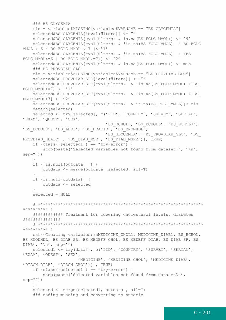
C - 201

### BS_GLYCEMIA mis = variables$MISSING[variables$VARNAME == ”BS_GLYCEMIA”] selected$BS_GLYCEMIA[!eval(filters)] <- ”” selected$BS_GLYCEMIA[eval(filters) & is.na(BS_FGLC_MMOL)] <- ’9’ selected$BS_GLYCEMIA[eval(filters) & !is.na(BS_FGLC_MMOL) & BS_FGLC_MMOL > 6 & BS_FGLC_MMOL < 7 ]<-’1’ selected$BS_GLYCEMIA[eval(filters) & !is.na(BS_FGLC_MMOL) & (BS_FGLC_MMOL<=6 | BS_FGLC_MMOL>=7)] <- ’2’ selected$BS_GLYCEMIA[eval(filters) & is.na(BS_FGLC_MMOL)] <- mis ### BS_PROVDIAB_GLC mis = variables$MISSING[variables$VARNAME == ”BS_PROVDIAB_GLC”] selected$BS_PROVDIAB_GLC[!eval(filters)] <- ”” selected$BS_PROVDIAB_GLC[eval(filters) & !is.na(BS_FGLC_MMOL) & BS_FGLC_MMOL>=7] <- ’1’ selected$BS_PROVDIAB_GLC[eval(filters) & !is.na(BS_FGLC_MMOL) & BS_FGLC_MMOL<7] <- ’2’ selected$BS_PROVDIAB_GLC[eval(filters) & is.na(BS_FGLC_MMOL)]<-mis detach(selected) selected <- try(selected[, c(’PID’, ’COUNTRY’, ’SURVEY’, ’SERIAL’, ’EXAM’, ’QUEST’, ’SEX’, ’BS_ECHOL’, ’BS_ECHOL6’, ’BS_ECHOL7’, ’BS_ECHOL8’, ’BS_LHDL’, ’BS_HRATIO’, ’BS_ENONHDL’, ’BS_GLYCEMIA’, ’BS_PROVDIAB_GLC’, ’BS_PROVDIAB_HBA1C’ , ’BS_DIAB_MSR’, ’BS_DIAB_MSR2’)], TRUE) if (class( selected1 ) == ”try-error”) { stop(paste(’Selected variables not found from dataset.’, ’\n’, sep=””)) } if (!is.null(outdata) ) { outdata <- merge(outdata, selected, all=T) } if (is.null(outdata)) { outdata <- selected } selected = NULL

# **************************************************************************** # ############ Treatment for lowering cholesterol levels, diabetes ############### # **************************************************************************** # cat(’Creating variables:\nMEDICINE_CHOL1, MEDICINE_DIAB1, BS_HCHOL, BS_HNONHDL, BS_DIAB_SR, BS_MEDEFF_CHOL, BS_MEDEFF_DIAB, BS_DIAB_SR, BS_DIAB’, ’\n’, sep=’’) selected1 <- try(data[ , c(’PID’, ’COUNTRY’, ’SURVEY’, ’SERIAL’, ’EXAM’, ’QUEST’, ’SEX’, ’MEDICINE’, ’MEDICINE_CHOL’, ’MEDICINE_DIAB’, ’DIAGN_DIAB’, ’DIAGN_CHOL’)] , TRUE) if (class( selected1 ) == ”try-error”) { stop(paste(’Selected variables not found from dataset\n’, sep=””)) } selected <- merge(selected1, outdata , all=T) ### coding missing and converting to numeric

C - 202

mis = variables$MISSING[variables$VARNAME == ”BS_CHOL_MMOL”] selected$BS_CHOL_MMOL = code_miss_numeric(selected, ’BS_CHOL_MMOL’, mis, irr, filter=filters ) mis = variables$MISSING[variables$VARNAME == ”BS_HDL_MMOL”] selected$BS_HDL_MMOL = code_miss_numeric(selected, ’BS_HDL_MMOL’, mis, irr, filter=filters ) mis = variables$MISSING[variables$VARNAME == ”BS_CHOLHDL_RATIO”] selected$BS_CHOLHDL_RATIO = code_miss_numeric(selected, ’BS_CHOLHDL_RATIO’, mis, irr, filter=filters ) mis = variables$MISSING[variables$VARNAME == ”BS_NONHDL”] selected$BS_NONHDL = code_miss_numeric(selected, ’BS_NONHDL’, mis, irr, filter=filters ) mis = variables$MISSING[variables$VARNAME == ”BS_HBA1C_MMOL”] selected$BS_HBA1C_MMOL = code_miss_numeric(selected, ’BS_HBA1C_MMOL’, mis, irr, filter=filters ) mis = variables$MISSING[variables$VARNAME == ”BS_FGLC_MMOL”] irr = ”.” selected$BS_FGLC_MMOL = code_miss_numeric(selected, ’BS_FGLC_MMOL’, mis, irr, filter=filters ) irr = ”” attach(selected) ### MEDICINE_CHOL1 mis = variables$MISSING[variables$VARNAME == ”MEDICINE_CHOL1”] selected$MEDICINE_CHOL1[!eval(filters)] <- irr selected$MEDICINE_CHOL1[eval(filters) & MEDICINE != ”1” ] <- ”.” selected$MEDICINE_CHOL1[eval(filters) & MEDICINE == ”1” & MEDICINE_CHOL == ”1” ] <- ”1” selected$MEDICINE_CHOL1[eval(filters) & ((MEDICINE == ”1” & MEDICINE_CHOL == ”2”) ) ] <- ”2” selected$MEDICINE_CHOL1[eval(filters) & (MEDICINE == ”1” & MEDICINE_CHOL != ”1” & MEDICINE_CHOL != ”2”) ] <- mis ###MEDICINE_DIAB1 mis = variables$MISSING[variables$VARNAME == ”MEDICINE_DIAB1”] selected$MEDICINE_DIAB1[!eval(filters)] <- irr selected$MEDICINE_DIAB1[eval(filters) & MEDICINE != ”1” ] <- ”.” selected$MEDICINE_DIAB1[eval(filters) & MEDICINE == ”1” & MEDICINE_DIAB == ”1” ] <- ”1” selected$MEDICINE_DIAB1[eval(filters) & ((MEDICINE == ”1” & MEDICINE_DIAB == ”2”) ) ] <- ”2” selected$MEDICINE_DIAB1[eval(filters) & (MEDICINE == ”1” & MEDICINE_DIAB != ”1” & MEDICINE_DIAB != ”2”) ] <- mis detach(selected) ## BS_HCHOL mis = variables$MISSING[variables$VARNAME == ”BS_HCHOL”] attach(selected) selected$BS_HCHOL[!eval(filters)] <- irr selected$BS_HCHOL[eval(filters) & (BS_CHOL_MMOL>=5 | MEDICINE_CHOL1==’1’) & MEDICINE != ”9” & MEDICINE_CHOL1 != ”9” & !is.na(BS_CHOL_MMOL) ] <- ”1” selected$BS_HCHOL[eval(filters) & BS_CHOL_MMOL<5 & (MEDICINE_CHOL1 != ”1” & MEDICINE_CHOL1 != ”9”) ] <- ”2” selected$BS_HCHOL[eval(filters) & is.na(BS_CHOL_MMOL) | MEDICINE_CHOL1 == ”9” & MEDICINE == ”9”] <- mis detach(selected) ## BS_MEDEFF_CHOL

C - 203

mis = variables$MISSING[variables$VARNAME == ”BS_MEDEFF_CHOL”] attach(selected) selected$BS_MEDEFF_CHOL[!eval(filters)] <- irr selected$BS_MEDEFF_CHOL[eval(filters) & MEDICINE_CHOL1 != ”1” ] <- ”.” selected$BS_MEDEFF_CHOL[eval(filters) & BS_CHOL_MMOL < 5 & MEDICINE_CHOL1 == ”1” ] <- ”1” selected$BS_MEDEFF_CHOL[eval(filters) & BS_CHOL_MMOL >= 5 & MEDICINE_CHOL1 == ”1” ] <- ”2” selected$BS_MEDEFF_CHOL[eval(filters) & is.na(BS_CHOL_MMOL) & MEDICINE_CHOL1 == ”1”] <- mis ## BS_MEDEFF_DIAB mis = variables$MISSING[variables$VARNAME == ”BS_MEDEFF_DIAB”] selected$BS_MEDEFF_DIAB[!eval(filters)] <- irr selected$BS_MEDEFF_DIAB[eval(filters) & MEDICINE_DIAB1 != ”1” ] <- ”.” selected$BS_MEDEFF_DIAB[eval(filters) & is.na(BS_HBA1C_MMOL) & !is.na(BS_FGLC_MMOL) & BS_FGLC_MMOL<6 & MEDICINE_DIAB1 == ”1” ] <- ”1” selected$BS_MEDEFF_DIAB[eval(filters) & !is.na(BS_HBA1C_MMOL) & BS_HBA1C_MMOL<48 & MEDICINE_DIAB1 == ”1” ] <- ”1” selected$BS_MEDEFF_DIAB[eval(filters) & is.na(BS_HBA1C_MMOL) & !is.na(BS_FGLC_MMOL) & BS_FGLC_MMOL>=6 & MEDICINE_DIAB1 == ”1” ] <- ”2” selected$BS_MEDEFF_DIAB[eval(filters) & !is.na(BS_HBA1C_MMOL) & BS_HBA1C_MMOL>=48 & MEDICINE_DIAB1 == ”1” ] <- ”2” selected$BS_MEDEFF_DIAB[eval(filters) & is.na(BS_FGLC_MMOL) & is.na(BS_HBA1C_MMOL) & MEDICINE_DIAB1 == ”1”] <- mis ### BS_HNONHDL mis = variables$MISSING[variables$VARNAME == ”BS_HNONHDL”] selected$BS_HNONHDL[!eval(filters)] <- irr selected$BS_HNONHDL[eval(filters) & (BS_NONHDL>3.5 | MEDICINE_CHOL1==’1’)]<-’1’ selected$BS_HNONHDL[eval(filters) & BS_NONHDL<=3.5 & MEDICINE_CHOL1==’2’]<-’2’ selected$BS_HNONHDL[eval(filters) & is.na(BS_NONHDL) & MEDICINE_CHOL1 != ”1” & MEDICINE_CHOL1 != ”2”] <-mis ### BS_DIAB_SR mis = variables$MISSING[variables$VARNAME == ”BS_DIAB_SR”] selected$BS_DIAB_SR[!eval(filters)] <- irr selected$BS_DIAB_SR[eval(filters) & (BS_DIAB_MSR==’1’ | DIAGN_DIAB==’1’)] <- ”1” selected$BS_DIAB_SR[eval(filters) & BS_DIAB_MSR==’2’ & DIAGN_DIAB==’2’] <- ”2” selected$BS_DIAB_SR[eval(filters) & BS_DIAB_MSR != ”1” & BS_DIAB_MSR != ”2” & DIAGN_DIAB != ”1” & DIAGN_DIAB != ”2”] <- mis ### BS_DIAB mis = variables$MISSING[variables$VARNAME == ”BS_DIAB”] selected$BS_DIAB[!eval(filters)] <- irr selected$BS_DIAB[eval(filters) & (BS_DIAB_MSR==’1’ | MEDICINE_DIAB1==’1’) ]<-’1’ selected$BS_DIAB[eval(filters) & BS_DIAB_MSR==’2’ & MEDICINE_DIAB1==’2’]<-’2’ selected$BS_DIAB[eval(filters) & BS_DIAB_MSR != ”1” & BS_DIAB_MSR != ”2” & MEDICINE_DIAB1 != ”1” & MEDICINE_DIAB1 != ”2”] <- mis detach(selected) attach(selected)

C - 204

### Medicines among population MEDICINE_DIAB_POP mis = variables$MISSING[variables$VARNAME == ”MEDICINE_DIAB_POP”] selected$MEDICINE_DIAB_POP[!eval(filters)] <- irr selected$MEDICINE_DIAB_POP[eval(filters) & MEDICINE_DIAB1 == ”1” ] <- ”1” selected$MEDICINE_DIAB_POP[eval(filters) & (MEDICINE_DIAB1 == ”2” | MEDICINE == ”2”) ] <- ”2” selected$MEDICINE_DIAB_POP[eval(filters) & ((MEDICINE == ”1” & MEDICINE_DIAB1 == ”9”) | (MEDICINE != ”1” & MEDICINE != ”2” ) ) ] <- mis ### Medicines among actual or potential MEDICINE_DIAB_ILL mis = variables$MISSING[variables$VARNAME == ”MEDICINE_DIAB_ILL”] selected$MEDICINE_DIAB_ILL[!eval(filters)] <- irr selected$MEDICINE_DIAB_ILL[eval(filters) & BS_DIAB != ”1” ] <- ”.” selected$MEDICINE_DIAB_ILL[eval(filters) & BS_DIAB == ”1” & MEDICINE_DIAB1 == ”1” ] <- ”1” selected$MEDICINE_DIAB_ILL[eval(filters) & ((BS_DIAB == ”1” & MEDICINE_DIAB1 == ”2”) | (BS_DIAB == ”1” & MEDICINE == ”2”)) ] <- ”2” selected$MEDICINE_DIAB_ILL[eval(filters) & (BS_DIAB == ”1” & MEDICINE_DIAB1 == ”9”) ] <- mis selected$MEDICINE_DIAB_ILL[eval(filters) & (BS_DIAB == ”1” & MEDICINE_DIAB1 == ”9” ) | (BS_DIAB == ”1” & MEDICINE == ”9”) ] <- ”.” ### Medicines among population MEDICINE_CHOL_POP mis = variables$MISSING[variables$VARNAME == ”MEDICINE_CHOL_POP”] selected$MEDICINE_CHOL_POP[!eval(filters)] <- irr selected$MEDICINE_CHOL_POP[eval(filters) & MEDICINE_CHOL1 == ”1” ] <- ”1” selected$MEDICINE_CHOL_POP[eval(filters) & (MEDICINE_CHOL1 == ”2” | MEDICINE == ”2”) ] <- ”2” selected$MEDICINE_CHOL_POP[eval(filters) & ((MEDICINE == ”1” & MEDICINE_CHOL1 == ”9”) | (MEDICINE != ”1” & MEDICINE != ”2” ) ) ] <- mis ### Medicines among actual or potential MEDICINE_CHOL_ILL mis = variables$MISSING[variables$VARNAME == ”MEDICINE_CHOL_ILL”] selected$MEDICINE_CHOL_ILL[!eval(filters)] <- irr selected$MEDICINE_CHOL_ILL[eval(filters) & BS_HCHOL != ”1” ] <- ”.” selected$MEDICINE_CHOL_ILL[eval(filters) & BS_HCHOL == ”1” & MEDICINE_CHOL1 == ”1” ] <- ”1” selected$MEDICINE_CHOL_ILL[eval(filters) & ((BS_HCHOL == ”1” & MEDICINE_CHOL1 == ”2”) | (BS_HCHOL == ”1” & MEDICINE == ”2”)) ] <- ”2” selected$MEDICINE_CHOL_ILL[eval(filters) & (BS_HCHOL == ”1” & MEDICINE_CHOL1 == ”9”) ] <- mis selected$MEDICINE_CHOL_ILL[eval(filters) & (BS_HCHOL == ”1” & MEDICINE_CHOL1 == ”9” ) | (BS_HCHOL == ”1” & MEDICINE == ”9”) ] <- ”.” #### Awareness of elevated cholestero BS_CHOL_AWARE mis = variables$MISSING[variables$VARNAME == ”BS_CHOL_AWARE”] selected$BS_CHOL_AWARE[!eval(filters)] <- irr selected$BS_CHOL_AWARE[eval(filters) & BS_HCHOL != ”1” ] <- ”.” selected$BS_CHOL_AWARE[eval(filters) & BS_HCHOL == ”1” & DIAGN_CHOL == ”1” ] <- ”1” selected$BS_CHOL_AWARE[eval(filters) & BS_HCHOL == ”1” & (DIAGN_CHOL == ”2” | DIAGN_CHOL == ”8” )] <- ”2” selected$BS_CHOL_AWARE[eval(filters) & BS_HCHOL == ”1” & DIAGN_CHOL != ”1” & DIAGN_CHOL != ”2” & DIAGN_CHOL != ”8”] <- mis detach(selected) #### BS_DIAB_AWARE attach(selected)

C - 205

mis = variables$MISSING[variables$VARNAME == ”BS_DIAB_AWARE”] selected$BS_DIAB_AWARE[!eval(filters)] <- irr selected$BS_DIAB_AWARE[eval(filters) & BS_DIAB != ”1” ] <- ”.” selected$BS_DIAB_AWARE[eval(filters) & BS_DIAB == ”1” & DIAGN_DIAB == ”1” ] <- ”1” selected$BS_DIAB_AWARE[eval(filters) & BS_DIAB == ”1” & (DIAGN_DIAB == ”2” | DIAGN_DIAB == ”8” )] <- ”2” selected$BS_DIAB_AWARE[eval(filters) & BS_DIAB == ”1” & DIAGN_DIAB != ”1” & DIAGN_DIAB != ”2” & DIAGN_DIAB != ”8”] <- mis #### BS_DIAB_SR_AWARE mis = variables$MISSING[variables$VARNAME == ”BS_DIAB_SR_AWARE”] selected$BS_DIAB_SR_AWARE[!eval(filters)] <- irr selected$BS_DIAB_SR_AWARE[eval(filters) & BS_DIAB_SR != ”1” ] <- ”.” selected$BS_DIAB_SR_AWARE[eval(filters) & BS_DIAB_SR == ”1” & DIAGN_DIAB == ”1” ] <- ”1” selected$BS_DIAB_SR_AWARE[eval(filters) & BS_DIAB_SR == ”1” & (DIAGN_DIAB == ”2” | DIAGN_DIAB == ”8” )] <- ”2” selected$BS_DIAB_SR_AWARE[eval(filters) & BS_DIAB_SR == ”1” & DIAGN_DIAB != ”1” & DIAGN_DIAB != ”2” & DIAGN_DIAB != ”8”] <- mis ### Optimal cholestero among those using drugs BS_CHOL_OPTIMAL mis = variables$MISSING[variables$VARNAME == ”BS_CHOL_OPTIMAL”] selected$BS_CHOL_OPTIMAL[!eval(filters)] <- irr selected$BS_CHOL_OPTIMAL[eval(filters) & MEDICINE_CHOL1 != ”1” ] <- ”.” selected$BS_CHOL_OPTIMAL[eval(filters) & MEDICINE_CHOL1 == ”1” & BS_ECHOL == ”2” ] <- ”1” selected$BS_CHOL_OPTIMAL[eval(filters) & MEDICINE_CHOL1 == ”1” & BS_ECHOL == ”1” ] <- ”2” selected$BS_CHOL_OPTIMAL[eval(filters) & MEDICINE_CHOL1 == ”1” & BS_ECHOL != ”1” & BS_ECHOL != ”2” ] <- mis detach(selected) selected <- try(selected[, c(’PID’, ’COUNTRY’, ’SURVEY’, ’SERIAL’,’EXAM’, ’QUEST’, ’SEX’, ’BS_HCHOL’, ’BS_HNONHDL’, ’MEDICINE_CHOL1’, ’BS_MEDEFF_CHOL’, ’MEDICINE_DIAB1’, ’BS_MEDEFF_DIAB’, ’BS_DIAB_SR’, ’BS_DIAB’, ’BS_CHOL_AWARE’, ’BS_DIAB_AWARE’, ’BS_DIAB_SR_AWARE’, ’MEDICINE_DIAB_POP’, ’MEDICINE_DIAB_ILL’, ’MEDICINE_CHOL_POP’, ’MEDICINE_CHOL_ILL’, ’BS_CHOL_OPTIMAL’, ’BS_GLC_OPTIMAL’)] , TRUE) if (class( selected ) == ”try-error”) { stop(paste(’Selected variables not found from dataset.’, ’\n’, sep=””)) } if (!is.null(outdata) ) { outdata <- merge(outdata, selected, all=T) } if (is.null(outdata)) { outdata <- selected } selected <- NULL tstop <- Sys.time() cat(’\nEHES_derived_variables_bs function call completed in ’, format(round(difftime(tstop, tstart, units=’mins’), digits=3), nsmall=3), ’.’, ’\n’, sep=’’) return(outdata)

C - 206

}

derived_variables_anthropometrics - to calculate derived variables for anthropometrics

derived_variables_anthropometrics <- function(data=NA, variables) { ### data = dataset, variables = definition table for variables tstart <- Sys.time() outdata=NULL if (is.null(data) ) { stop(”\n***ERROR:***\n No data given. Execution halted.”) } cat(’Creating variables:\nBMI, WAIST_LARGE, BMI_OVERWEIGHT, BMI_OBESE, BMI_CATEGORY’, ’\n\n’, sep=’’) selected <- try(data[, c(’PID’, ’COUNTRY’, ’SURVEY’, ’SERIAL’, ’EXAM’, ’QUEST’, ’SEX’, ’WEIGHT’, ’HEIGHT’, ’WAIST’)] , TRUE) if (class( selected ) == ”try-error”) { stop(paste(’Selected variables not found from dataset \n’, sep=””)) } # to filter the participants filters <- expression(EXAM == ’1’ | QUEST == ’1’) attach(selected) selected = selected[eval(filters),] detach(selected) irr = ”” ## Coding missing values and converting to numeric mis = variables$MISSING[variables$VARNAME == ”WEIGHT”] selected$WEIGHT = code_miss_numeric(selected, ’WEIGHT’, mis, irr, filter=filters ) mis = variables$MISSING[variables$VARNAME == ”HEIGHT”] selected$HEIGHT = code_miss_numeric(selected, ’HEIGHT’, mis, irr, filter=filters ) mis = variables$MISSING[variables$VARNAME == ”WAIST”] selected$WAIST = code_miss_numeric(selected, ’WAIST’, mis, irr, filter=filters ) attach(selected) ### BMI mis = variables$MISSING[variables$VARNAME == ”BMI”] selected$BMI[eval(filters) ] <- format(round(selected[eval(filters), c(’WEIGHT’)] / (( selected[eval(filters) , c(’HEIGHT’)]/100)^2) , 2), nsmall=2, trim=T) selected$BMI[!eval(filters)] <- irr selected$BMI[eval(filters) & (is.na(WEIGHT) | is.na(HEIGHT))] <- mis ## WAIST_LARGE mis = variables$MISSING[variables$VARNAME == ”WAIST_LARGE”] selected$WAIST_LARGE[!eval(filters)] = irr selected$WAIST_LARGE[eval(filters) & SEX==’1’ & WAIST>102]<- ’1’ selected$WAIST_LARGE[eval(filters) & SEX==’2’ & WAIST>88]<- ’1’ selected$WAIST_LARGE[eval(filters) & SEX==’1’ & WAIST<=102]<- ’2’ selected$WAIST_LARGE[eval(filters) & SEX==’2’ & WAIST<=88]<- ’2’ selected$WAIST_LARGE[eval(filters) & is.na(WAIST) & SEX != ”1” & SEX != ”2” ]<- mis

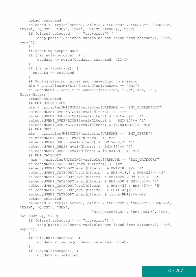
C - 207

detach(selected) selected <- try(selected[, c(’PID’, ’COUNTRY’, ’SURVEY’, ’SERIAL’, ’EXAM’, ’QUEST’, ’SEX’, ’BMI’, ’WAIST_LARGE’)], TRUE) if (class( selected ) == ”try-error”) { stop(paste(’Selected variables not found from dataset.’, ’\n’, sep=””)) } ## creating output data if (!is.null(outdata) ) { outdata <- merge(outdata, selected, all=T) } if (is.null(outdata)) { outdata <- selected } ## Coding missing values and converting to numeric mis = variables$MISSING[variables$VARNAME == ”BMI”] selected$BMI = code_miss_numeric(selected, ’BMI’, mis, irr, filter=filters ) attach(selected) ## BMI_OVERWEIGHT mis = variables$MISSING[variables$VARNAME == ”BMI_OVERWEIGHT”] selected$BMI_OVERWEIGHT[!eval(filters)] <- irr selected$BMI_OVERWEIGHT[eval(filters) & BMI>=25]<- ’1’ selected$BMI_OVERWEIGHT[eval(filters) & BMI<25]<- ’2’ selected$BMI_OVERWEIGHT[eval(filters) & is.na(BMI)]<- mis ## BMI_OBESE mis = variables$MISSING[variables$VARNAME == ”BMI_OBESE”] selected$BMI_OBESE[!eval(filters)] <- mis selected$BMI_OBESE[eval(filters) & BMI>=30]<- ’1’ selected$BMI_OBESE[eval(filters) & BMI<30]<- ’2’ selected$BMI_OBESE[eval(filters) & is.na(BMI)]<- mis ## BMI_CATEGORY mis = variables$MISSING[variables$VARNAME == ”BMI_CATEGORY”] selected$BMI_CATEGORY[!eval(filters)] <- irr selected$BMI_CATEGORY[eval(filters) & BMI<18.5]<- ’1’ selected$BMI_CATEGORY[eval(filters) & BMI>=18.5 & BMI<25]<- ’2’ selected$BMI_CATEGORY[eval(filters) & BMI>=25 & BMI<30]<- ’3’ selected$BMI_CATEGORY[eval(filters) & BMI>=30 & BMI<35]<- ’4’ selected$BMI_CATEGORY[eval(filters) & BMI>=35 & BMI<40]<- ’5’ selected$BMI_CATEGORY[eval(filters) & BMI>=40]<- ’6’ selected$BMI_CATEGORY[eval(filters) & is.na(BMI)]<- mis detach(selected) selected <- try(selected[, c(’PID’, ’COUNTRY’, ’SURVEY’, ’SERIAL’, ’EXAM’, ’QUEST’, ’SEX’, ’BMI_OVERWEIGHT’, ’BMI_OBESE’, ’BMI_CATEGORY’)], TRUE) if (class( selected ) == ”try-error”) { stop(paste(’Selected variables not found from dataset.’, ’\n’, sep=””)) } if (!is.null(outdata) ) { outdata <- merge(outdata, selected, all=T) } if (is.null(outdata)) { outdata <- selected

C - 208

} selected = NULL

# **************************************************************************** # ############ self reported height, weight, BMI ############### # **************************************************************************** # cat(’Creating variables:\nBMI_SR, HEIGHT_DIFF, WEIGHT_DIFF, BMI_DIFF, BMI_OVERWEIGHT_SR, BMI_OBESE_SR, BMI_CATEGORY_SR, PREGN1’, ’\n’, sep=’’) selected1 <- try(data[ , c(’PID’, ’COUNTRY’, ’SURVEY’, ’SERIAL’, ’EXAM’, ’QUEST’, ’SEX’, ’SHEIGHT’, ’SWEIGHT’, ’PREGN’)] , TRUE) if (class( selected1 ) == ”try-error”) { stop(paste(’Selected variables not found from dataset\n’, sep=””)) } selected2 <- try(data[ , c(’PID’, ’COUNTRY’, ’SURVEY’, ’SERIAL’, ’ELIG’, ’EXAM’, ’QUEST’, ’SEX’, ’HEIGHT’, ’WEIGHT’)] , TRUE) if (class( selected2 ) == ”try-error”) { stop(paste(’Selected variables not found from dataset\n’, sep=””)) } selected <- merge(selected1, outdata , all=T) selected <- merge(selected, selected2 , all=T) selected1=NULL selected2=NULL ### coding missing and converting to numeric mis = variables$MISSING[variables$VARNAME == ”WEIGHT”] selected$WEIGHT = code_miss_numeric(selected, ’WEIGHT’, mis, irr, filter=filters ) mis = variables$MISSING[variables$VARNAME == ”HEIGHT”] selected$HEIGHT = code_miss_numeric(selected, ’HEIGHT’, mis, irr, filter=filters ) mis = variables$MISSING[variables$VARNAME == ”BMI”] selected$BMI = code_miss_numeric(selected, ’BMI’, mis, irr, filter=filters ) mis = c(variables$MISSING[variables$VARNAME == ”SWEIGHT”], variables$DONTKNOW[variables$VARNAME == ”SWEIGHT”]) selected$SWEIGHT = code_miss_numeric(selected, ’SWEIGHT’, mis, irr, filter=filters ) mis = c(variables$MISSING[variables$VARNAME == ”SHEIGHT”], variables$DONTKNOW[variables$VARNAME == ”SHEIGHT”]) selected$SHEIGHT = code_miss_numeric(selected, ’SHEIGHT’, mis, irr, filter=filters ) attach(selected) ### BMI_SR mis = variables$MISSING[variables$VARNAME == ”BMI_SR”] selected$BMI_SR[eval(filters) ] <- format(round(selected[eval(filters) , c(’SWEIGHT’)]/((selected[eval(filters), c(’SHEIGHT’)]/100)^2 ), 2), nsmall=2, trim=T) selected$BMI_SR[!eval(filters)] <- irr selected$BMI_SR[eval(filters) & (is.na(SWEIGHT)|is.na(SHEIGHT))]<-

C - 209

mis ### HEIGHT_DIFF mis = variables$MISSING[variables$VARNAME == ”HEIGHT_DIFF”] selected$HEIGHT_DIFF[eval(filters) ]<- format(round(selected[eval(filters) ,c(’SHEIGHT’)] - selected[eval(filters) ,c(’HEIGHT’)], 2), nsmall=2, trim=T) selected$HEIGHT_DIFF[!eval(filters)] <- irr selected$HEIGHT_DIFF[eval(filters) & (is.na(HEIGHT)|is.na(SHEIGHT))]<- mis ### WEIGHT_DIFF mis = variables$MISSING[variables$VARNAME == ”WEIGHT_DIFF”] selected$WEIGHT_DIFF[eval(filters)]<- format(round(selected[eval(filters) ,c(’SWEIGHT’)] - selected[eval(filters) ,c(’WEIGHT’)] , 2), nsmall=2, trim=T) selected$WEIGHT_DIFF[!eval(filters)] <- irr selected$WEIGHT_DIFF[eval(filters) & (is.na(WEIGHT)|is.na(SWEIGHT))]<- mis ### PREGN1 mis = variables$MISSING[variables$VARNAME == ”PREGN1”] selected$PREGN1[!eval(filters)] <- irr selected$PREGN1[eval(filters) & SEX != ”2”]<- ”.” selected$PREGN1[eval(filters) & SEX == ”2”]<- selected$PREGN[eval(filters) & SEX == ”2”] selected$PREGN1[eval(filters) & SEX == ”2” & !(PREGN %in% c(”1”,”2”))] <- mis detach(selected) selected <- try(selected[, c(’PID’, ’COUNTRY’, ’SURVEY’, ’SERIAL’, ’EXAM’, ’QUEST’, ’SEX’, ’BMI_SR’, ’HEIGHT_DIFF’, ’WEIGHT_DIFF’, ’PREGN1’)], TRUE) if (class( selected ) == ”try-error”) { stop(paste(’Selected variables not found from dataset.’, ’\n’, sep=””)) } if (!is.null(outdata) ) { outdata <- merge(outdata, selected, all=T) } if (is.null(outdata)) { outdata <- selected } selected = outdata ### coding missing and converting to numeric mis = variables$MISSING[variables$VARNAME == ”BMI”] selected$BMI = code_miss_numeric(selected, ’BMI’, mis, irr, filter=filters ) mis = variables$MISSING[variables$VARNAME == ”BMI_SR”] selected$BMI_SR = code_miss_numeric(selected, ’BMI_SR’, mis, irr, filter=filters ) attach(selected) ### BMI_DIFF mis = variables$MISSING[variables$VARNAME == ”BMI_DIFF”] selected$BMI_DIFF[eval(filters) ]<- format(round(selected[eval(filters),c(’BMI_SR’)] - selected[eval(filters),c(’BMI’)] , 2), nsmall=2, trim=T) selected$BMI_DIFF[!eval(filters)] <- irr

C - 210

selected$BMI_DIFF[eval(filters) & (is.na(BMI)|is.na(BMI_SR))]<- mis ## BMI_OVERWEIGHT_SR mis = variables$MISSING[variables$VARNAME == ”BMI_OVERWEIGHT_SR”] selected$BMI_OVERWEIGHT_SR[!eval(filters)] <- irr selected$BMI_OVERWEIGHT_SR[eval(filters) & BMI_SR>=25]<- ’1’ selected$BMI_OVERWEIGHT_SR[eval(filters) & BMI_SR<25]<- ’2’ selected$BMI_OVERWEIGHT_SR[eval(filters) & is.na(BMI_SR)]<- mis ## BMI_OBESE_SR mis = variables$MISSING[variables$VARNAME == ”BMI_OBESE_SR”] selected$BMI_OBESE_SR[!eval(filters)] <- irr selected$BMI_OBESE_SR[eval(filters) & BMI_SR>=30]<- ’1’ selected$BMI_OBESE_SR[eval(filters) & BMI_SR<30]<- ’2’ selected$BMI_OBESE_SR[eval(filters) & is.na(BMI_SR)]<- mis ## BMI_CATEGORY_SR mis = variables$MISSING[variables$VARNAME == ”BMI_CATEGORY_SR”] selected$BMI_OBESE_SR[!eval(filters)] <- irr selected$BMI_CATEGORY_SR[eval(filters) & BMI_SR<18.5]<- ’1’ selected$BMI_CATEGORY_SR[ eval(filters) & BMI_SR>=18.5 & BMI_SR<25]<- ’2’ selected$BMI_CATEGORY_SR[eval(filters) & BMI_SR>=25 & BMI_SR<30]<- ’3’ selected$BMI_CATEGORY_SR[ eval(filters) & BMI_SR>=30 & BMI_SR<35]<- ’4’ selected$BMI_CATEGORY_SR[eval(filters) & BMI_SR>=35 & BMI_SR<40]<- ’5’ selected$BMI_CATEGORY_SR[eval(filters) & BMI_SR>=40]<- ’6’ selected$BMI_CATEGORY_SR[eval(filters) & is.na(BMI_SR)]<- mis detach(selected) selected <- try(selected[, c(’PID’, ’COUNTRY’, ’SURVEY’, ’SERIAL’, ’EXAM’, ’QUEST’, ’SEX’, ’BMI_DIFF’, ’BMI_OVERWEIGHT_SR’, ’BMI_OBESE_SR’, ’BMI_CATEGORY_SR’, ’PREGN1’)] , TRUE) if (class( selected ) == ”try-error”) { stop(paste(’Selected variables not found from dataset.’, ’\n’, sep=””)) } if (!is.null(outdata) ) { outdata <- merge(outdata, selected, all=T) } if (is.null(outdata)) { outdata <- selected } selected <- NULL tstop <- Sys.time() cat(’\nEHES_derived_variables_anthropometrics function call completed in ’, format(round(difftime(tstop, tstart, units=’mins’), digits=3), nsmall=3), ’.’, ’\n’, sep=’’) return(outdata)}

derived_variables_smoking - to calculate derived variables for smok-ing

derived_variables_smoking <- function(data=NA, variables) { ### data = dataset, variables = definition table for variables

C - 211

tstart <- Sys.time() outdata=NULL if (is.null(data) ) { stop(”\n***ERROR:***\n No data given. Execution halted.”) } cat(’Creating variables:\nSMOKEY, NUM_... and SMOKE_... variables’, ’\n\n’, sep=’’) selected <- try(data[, c(’PID’, ’COUNTRY’, ’SURVEY’, ’SERIAL’, ’EXAM’, ’QUEST’, ’SMOKE’, ’SMOKE_EVER’, ’SMOKE_YEARS’, ’SMOKE_CIGSM’, ’NUM_CIGSM’, ’SMOKE_CIGSH’, ’NUM_CIGSH’, ’SMOKE_CIGARS’, ’NUM_CIGARS’, ’SMOKE_PIPE’, ’NUM_PIPE’, ’SMOKE_OTHER’, ’NUM_OTHER’)] , TRUE) if (class( selected ) == ”try-error”) { stop(paste(’Selected variables not found from dataset \n’, sep=””)) } # to filter the participants filters <- expression(EXAM == ’1’ | QUEST == ’1’) attach(selected) selected = selected[eval(filters),] detach(selected) irr = ”” mis = variables$MISSING[variables$VARNAME == ”SMOKEY”] attach(selected) selected$SMOKEY[!eval(filters)] <- irr selected$SMOKEY[eval(filters) & (SMOKE==’1’|SMOKE_EVER==’1’)] <- selected[eval(filters) & (SMOKE==’1’|SMOKE_EVER==’1’), c(’SMOKE_YEARS’)] selected$SMOKEY[eval(filters) & (SMOKE_EVER==’2’ & (SMOKE==’2’ | SMOKE==’3’))] <- ’0’ selected$SMOKEY[eval(filters) & SMOKE_YEARS ==’99’ | (SMOKE != ’1’ & SMOKE != ’2’ & SMOKE != ’3’ & SMOKE_EVER != ’1’ & SMOKE_EVER != ’2’) ]<-mis ## SMOKE_... variables using filters irr = variables$IRRELEVANT[variables$VARNAME == ”SMOKE_CIGSM1”] mis = variables$MISSING[variables$VARNAME == ”SMOKE_CIGSM1”] selected$SMOKE_CIGSM1[!eval(filters)] <- ”” selected$SMOKE_CIGSM1[eval(filters) & SMOKE != ’1’] <- irr selected$SMOKE_CIGSM1[eval(filters) & SMOKE == ’1’] <- selected$SMOKE_CIGSM[eval(filters) & SMOKE == ’1’] selected$SMOKE_CIGSM1[eval(filters) & SMOKE == ’1’ & SMOKE_CIGSM != ’1’ & SMOKE_CIGSM != ”2”]<-mis irr = variables$IRRELEVANT[variables$VARNAME == ”SMOKE_CIGSH1”] mis = variables$MISSING[variables$VARNAME == ”SMOKE_CIGSH1”] selected$SMOKE_CIGSH1[!eval(filters)] <- ”” selected$SMOKE_CIGSH1[eval(filters) & SMOKE != ’1’] <- irr selected$SMOKE_CIGSH1[eval(filters) & SMOKE == ’1’] <- selected$SMOKE_CIGSH[eval(filters) & SMOKE == ’1’] selected$SMOKE_CIGSH1[eval(filters) & SMOKE == ’1’ & SMOKE_CIGSH != ’1’ & SMOKE_CIGSH != ”2”]<-mis irr = variables$IRRELEVANT[variables$VARNAME == ”SMOKE_CIGARS1”] mis = variables$MISSING[variables$VARNAME == ”SMOKE_CIGARS1”] selected$SMOKE_CIGARS1[!eval(filters)] <- ”” selected$SMOKE_CIGARS1[eval(filters) & SMOKE != ’1’] <- irr selected$SMOKE_CIGARS1[eval(filters) & SMOKE == ’1’] <- selected$SMOKE_CIGARS[eval(filters) & SMOKE == ’1’]

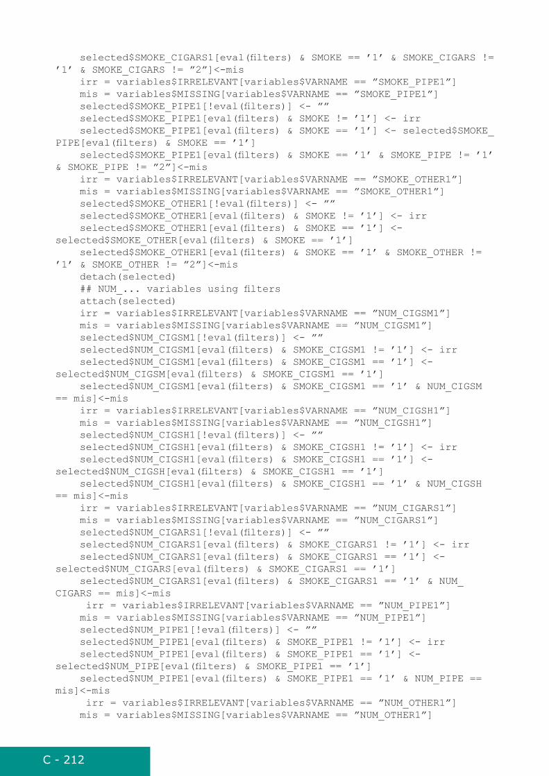
C - 212

selected$SMOKE_CIGARS1[eval(filters) & SMOKE == ’1’ & SMOKE_CIGARS != ’1’ & SMOKE_CIGARS != ”2”]<-mis irr = variables$IRRELEVANT[variables$VARNAME == ”SMOKE_PIPE1”] mis = variables$MISSING[variables$VARNAME == ”SMOKE_PIPE1”] selected$SMOKE_PIPE1[!eval(filters)] <- ”” selected$SMOKE_PIPE1[eval(filters) & SMOKE != ’1’] <- irr selected$SMOKE_PIPE1[eval(filters) & SMOKE == ’1’] <- selected$SMOKE_PIPE[eval(filters) & SMOKE == ’1’] selected$SMOKE_PIPE1[eval(filters) & SMOKE == ’1’ & SMOKE_PIPE != ’1’ & SMOKE_PIPE != ”2”]<-mis irr = variables$IRRELEVANT[variables$VARNAME == ”SMOKE_OTHER1”] mis = variables$MISSING[variables$VARNAME == ”SMOKE_OTHER1”] selected$SMOKE_OTHER1[!eval(filters)] <- ”” selected$SMOKE_OTHER1[eval(filters) & SMOKE != ’1’] <- irr selected$SMOKE_OTHER1[eval(filters) & SMOKE == ’1’] <- selected$SMOKE_OTHER[eval(filters) & SMOKE == ’1’] selected$SMOKE_OTHER1[eval(filters) & SMOKE == ’1’ & SMOKE_OTHER != ’1’ & SMOKE_OTHER != ”2”]<-mis detach(selected) ## NUM_... variables using filters attach(selected) irr = variables$IRRELEVANT[variables$VARNAME == ”NUM_CIGSM1”] mis = variables$MISSING[variables$VARNAME == ”NUM_CIGSM1”] selected$NUM_CIGSM1[!eval(filters)] <- ”” selected$NUM_CIGSM1[eval(filters) & SMOKE_CIGSM1 != ’1’] <- irr selected$NUM_CIGSM1[eval(filters) & SMOKE_CIGSM1 == ’1’] <- selected$NUM_CIGSM[eval(filters) & SMOKE_CIGSM1 == ’1’] selected$NUM_CIGSM1[eval(filters) & SMOKE_CIGSM1 == ’1’ & NUM_CIGSM == mis]<-mis irr = variables$IRRELEVANT[variables$VARNAME == ”NUM_CIGSH1”] mis = variables$MISSING[variables$VARNAME == ”NUM_CIGSH1”] selected$NUM_CIGSH1[!eval(filters)] <- ”” selected$NUM_CIGSH1[eval(filters) & SMOKE_CIGSH1 != ’1’] <- irr selected$NUM_CIGSH1[eval(filters) & SMOKE_CIGSH1 == ’1’] <- selected$NUM_CIGSH[eval(filters) & SMOKE_CIGSH1 == ’1’] selected$NUM_CIGSH1[eval(filters) & SMOKE_CIGSH1 == ’1’ & NUM_CIGSH == mis]<-mis irr = variables$IRRELEVANT[variables$VARNAME == ”NUM_CIGARS1”] mis = variables$MISSING[variables$VARNAME == ”NUM_CIGARS1”] selected$NUM_CIGARS1[!eval(filters)] <- ”” selected$NUM_CIGARS1[eval(filters) & SMOKE_CIGARS1 != ’1’] <- irr selected$NUM_CIGARS1[eval(filters) & SMOKE_CIGARS1 == ’1’] <- selected$NUM_CIGARS[eval(filters) & SMOKE_CIGARS1 == ’1’] selected$NUM_CIGARS1[eval(filters) & SMOKE_CIGARS1 == ’1’ & NUM_CIGARS == mis]<-mis irr = variables$IRRELEVANT[variables$VARNAME == ”NUM_PIPE1”] mis = variables$MISSING[variables$VARNAME == ”NUM_PIPE1”] selected$NUM_PIPE1[!eval(filters)] <- ”” selected$NUM_PIPE1[eval(filters) & SMOKE_PIPE1 != ’1’] <- irr selected$NUM_PIPE1[eval(filters) & SMOKE_PIPE1 == ’1’] <- selected$NUM_PIPE[eval(filters) & SMOKE_PIPE1 == ’1’] selected$NUM_PIPE1[eval(filters) & SMOKE_PIPE1 == ’1’ & NUM_PIPE == mis]<-mis irr = variables$IRRELEVANT[variables$VARNAME == ”NUM_OTHER1”] mis = variables$MISSING[variables$VARNAME == ”NUM_OTHER1”]

C - 213

selected$NUM_OTHER1[!eval(filters)] <- ”” selected$NUM_OTHER1[eval(filters) & SMOKE_OTHER1 != ’1’] <- irr selected$NUM_OTHER1[eval(filters) & SMOKE_OTHER1 == ’1’] <- selected$NUM_OTHER[eval(filters) & SMOKE_OTHER1 == ’1’] selected$NUM_OTHER1[eval(filters) & SMOKE_OTHER1 == ’1’ & NUM_OTHER == mis]<-mis ## SMOKE_EVER1 irr = variables$IRRELEVANT[variables$VARNAME == ”SMOKE_EVER1”] mis = variables$MISSING[variables$VARNAME == ”SMOKE_EVER1”] selected$SMOKE_EVER1[!eval(filters)] <- ”” selected$SMOKE_EVER1[eval(filters) & (SMOKE == ’1’ | SMOKE == ’’)] <- irr selected$SMOKE_EVER1[eval(filters) & SMOKE != ’1’ & SMOKE != ’’] <- selected$SMOKE_EVER[eval(filters) & SMOKE != ’1’ & SMOKE != ’’] selected$SMOKE_EVER1[eval(filters) & SMOKE != ’1’ & SMOKE_EVER == mis] <-mis detach(selected) attach(selected) ### SMOKE_YEARS1 irr = variables$IRRELEVANT[variables$VARNAME == ”SMOKE_YEARS1”] mis = variables$MISSING[variables$VARNAME == ”SMOKE_YEARS1”] selected$SMOKE_YEARS1[!eval(filters)] <- ”” selected$SMOKE_YEARS1[eval(filters) & SMOKE != ’1’ & SMOKE_EVER1 != ’1’] <- irr selected$SMOKE_YEARS1[eval(filters) & (SMOKE == ’1’ | SMOKE_EVER1 == ’1’)] <- selected$SMOKE_YEARS[eval(filters) & (SMOKE == ’1’ | SMOKE_EVER1 == ’1’)] selected$SMOKE_YEARS1[eval(filters) & (SMOKE == ’1’ | SMOKE_EVER1 == ’1’) & SMOKE_YEARS == mis] <-mis detach(selected) selected <- try(selected[, c(’PID’, ’COUNTRY’, ’SURVEY’, ’SERIAL’, ’EXAM’, ’QUEST’, ’SMOKEY’, ’SMOKE_CIGSM1’, ’NUM_CIGSM1’, ’SMOKE_CIGSH1’, ’NUM_CIGSH1’, ’SMOKE_CIGARS1’, ’NUM_CIGARS1’, ’SMOKE_PIPE1’, ’NUM_PIPE1’, ’SMOKE_OTHER1’, ’NUM_OTHER1’, ’SMOKE_EVER1’, ’SMOKE_YEARS1’)] , TRUE) if (class( selected ) == ”try-error”) { stop(paste(’Selected variables not found from dataset.’, ’\n’, sep=””)) } if (!is.null(outdata) ) { outdata <- merge(outdata, selected, all=T) } if (is.null(outdata)) { outdata <- selected } selected <- NULL tstop <- Sys.time() cat(’EHES_derived_variables_smoking function call completed in ’, format(round(difftime(tstop, tstart, units=’mins’), digits=3), nsmall=3), ’.’, ’\n\n’, sep=’’) return(outdata)}

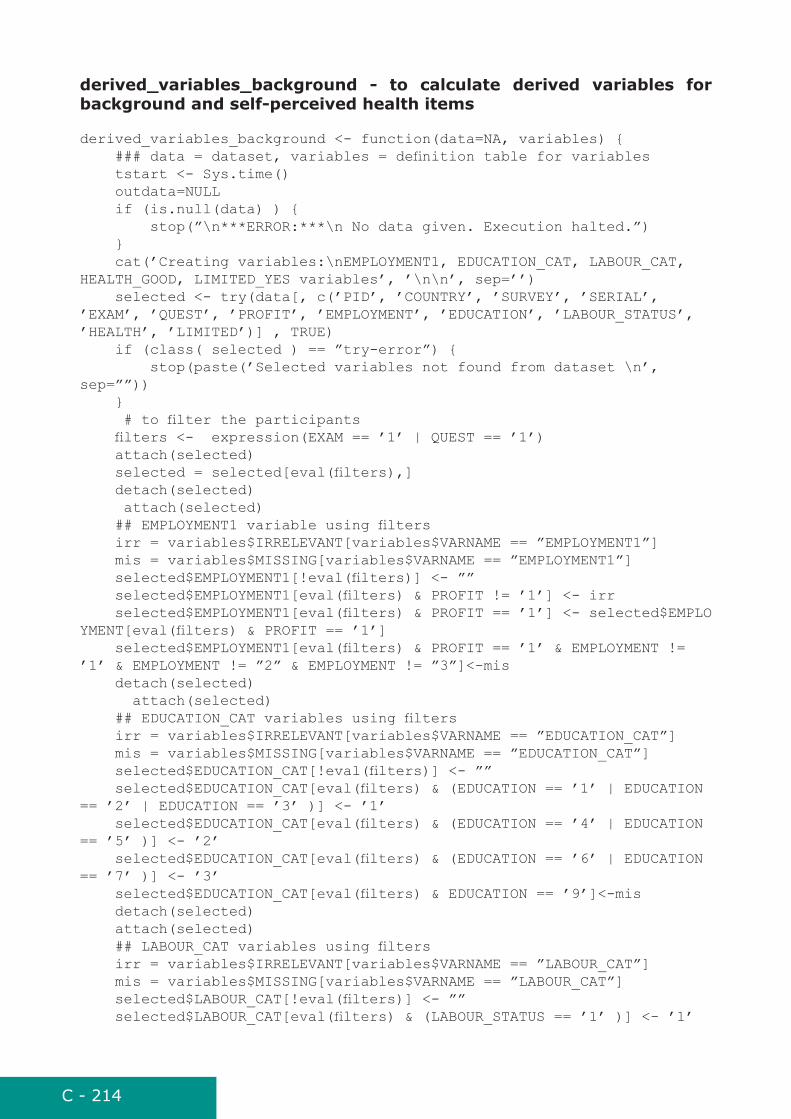
C - 214

derived_variables_background - to calculate derived variables for background and self-perceived health items

derived_variables_background <- function(data=NA, variables) { ### data = dataset, variables = definition table for variables tstart <- Sys.time() outdata=NULL if (is.null(data) ) { stop(”\n***ERROR:***\n No data given. Execution halted.”) } cat(’Creating variables:\nEMPLOYMENT1, EDUCATION_CAT, LABOUR_CAT, HEALTH_GOOD, LIMITED_YES variables’, ’\n\n’, sep=’’) selected <- try(data[, c(’PID’, ’COUNTRY’, ’SURVEY’, ’SERIAL’, ’EXAM’, ’QUEST’, ’PROFIT’, ’EMPLOYMENT’, ’EDUCATION’, ’LABOUR_STATUS’, ’HEALTH’, ’LIMITED’)] , TRUE) if (class( selected ) == ”try-error”) { stop(paste(’Selected variables not found from dataset \n’, sep=””)) } # to filter the participants filters <- expression(EXAM == ’1’ | QUEST == ’1’) attach(selected) selected = selected[eval(filters),] detach(selected) attach(selected) ## EMPLOYMENT1 variable using filters irr = variables$IRRELEVANT[variables$VARNAME == ”EMPLOYMENT1”] mis = variables$MISSING[variables$VARNAME == ”EMPLOYMENT1”] selected$EMPLOYMENT1[!eval(filters)] <- ”” selected$EMPLOYMENT1[eval(filters) & PROFIT != ’1’] <- irr selected$EMPLOYMENT1[eval(filters) & PROFIT == ’1’] <- selected$EMPLOYMENT[eval(filters) & PROFIT == ’1’] selected$EMPLOYMENT1[eval(filters) & PROFIT == ’1’ & EMPLOYMENT != ’1’ & EMPLOYMENT != ”2” & EMPLOYMENT != ”3”]<-mis detach(selected) attach(selected) ## EDUCATION_CAT variables using filters irr = variables$IRRELEVANT[variables$VARNAME == ”EDUCATION_CAT”] mis = variables$MISSING[variables$VARNAME == ”EDUCATION_CAT”] selected$EDUCATION_CAT[!eval(filters)] <- ”” selected$EDUCATION_CAT[eval(filters) & (EDUCATION == ’1’ | EDUCATION == ’2’ | EDUCATION == ’3’ )] <- ’1’ selected$EDUCATION_CAT[eval(filters) & (EDUCATION == ’4’ | EDUCATION == ’5’ )] <- ’2’ selected$EDUCATION_CAT[eval(filters) & (EDUCATION == ’6’ | EDUCATION == ’7’ )] <- ’3’ selected$EDUCATION_CAT[eval(filters) & EDUCATION == ’9’]<-mis detach(selected) attach(selected) ## LABOUR_CAT variables using filters irr = variables$IRRELEVANT[variables$VARNAME == ”LABOUR_CAT”] mis = variables$MISSING[variables$VARNAME == ”LABOUR_CAT”] selected$LABOUR_CAT[!eval(filters)] <- ”” selected$LABOUR_CAT[eval(filters) & (LABOUR_STATUS == ’1’ )] <- ’1’

C - 215

selected$LABOUR_CAT[eval(filters) & (LABOUR_STATUS == ’2’ )] <- ’2’ selected$LABOUR_CAT[eval(filters) & (LABOUR_STATUS == ’3’ | LABOUR_STATUS == ’4’ | LABOUR_STATUS == ’5’ | LABOUR_STATUS == ’6’| LABOUR_STATUS == ’7’ | LABOUR_STATUS == ’8’ )] <- ’3’ selected$LABOUR_CAT[eval(filters) & LABOUR_STATUS == ’9’]<-mis ## HEALTH_GOOD notknown = variables$DONTKNOW[variables$VARNAME == ”HEALTH_GOOD”] mis = variables$MISSING[variables$VARNAME == ”HEALTH_GOOD”] selected$HEALTH_GOOD[!eval(filters)] <- ”” selected$HEALTH_GOOD[eval(filters) & (HEALTH == ’1’ | HEALTH == ’2’)] <- ’1’ selected$HEALTH_GOOD[eval(filters) & (HEALTH != ’1’ & HEALTH != ’2’ & HEALTH != notknown & HEALTH != mis)] <- ’2’ selected$HEALTH_GOOD[eval(filters) & (HEALTH == notknown)] <- notknown selected$HEALTH_GOOD[eval(filters) & HEALTH == mis]<-mis ## LIMITED_YES notknown = variables$DONTKNOW[variables$VARNAME == ”LIMITED_YES”] mis = variables$MISSING[variables$VARNAME == ”LIMITED_YES”] selected$LIMITED_YES[!eval(filters)] <- ”” selected$LIMITED_YES[eval(filters) & (LIMITED == ’1’ | LIMITED == ’2’)] <- ’1’ selected$LIMITED_YES[eval(filters) & (LIMITED != ’1’ & LIMITED != ’2’ & LIMITED != notknown & LIMITED != mis)] <- ’2’ selected$LIMITED_YES[eval(filters) & (LIMITED == notknown)] <- notknown selected$LIMITED_YES[eval(filters) & LIMITED == mis]<-mis detach(selected) selected <- try(selected[, c(’PID’, ’COUNTRY’, ’SURVEY’, ’SERIAL’, ’EXAM’, ’QUEST’, ’EMPLOYMENT1’, ’EDUCATION_CAT’, ’LABOUR_CAT’, ’HEALTH_GOOD’, ’LIMITED_YES’)] , TRUE) if (class( selected ) == ”try-error”) { stop(paste(’Selected variables not found from dataset.’, ’\n’, sep=””)) } if (!is.null(outdata) ) { outdata <- merge(outdata, selected, all=T) } if (is.null(outdata)) { outdata <- selected } selected <- NULL tstop <- Sys.time() cat(’EHES_derived_variables_background function call completed in ’, format(round(difftime(tstop, tstart, units=’mins’), digits=3), nsmall=3), ’.’, ’\n\n’, sep=’’) return(outdata)}

derived_variables_elig - to calculate derived variables for eligibility and consent items

derived_variables_elig <- function(data=NA, variables) { ### data = dataset, variables = definition table for variables

C - 216

tstart <- Sys.time() outdata=NULL if (is.null(data) ) { stop(”\n***ERROR:***\n No data given. Execution halted.”) } cat(’Creating variables:\nEXAM1, QUEST1, REASON1, EXAM_REF1, EXAM_NOAPP1, QUEST_REF1, CONSENT_...1, variables’, ’\n\n’, sep=’’) selected <- try(data[, c(’PID’, ’COUNTRY’, ’SURVEY’, ’SERIAL’, ’ELIG’, ’EXAM’, ’QUEST’, ’REASON’, ’EXAM_REF’, ’EXAM_NOAPP’, ’QUEST_REF’, ’CONSENT_ANTR’, ’CONSENT_BP’, ’CONSENT_BS’, ’CONSENT_LIPID’, ’CONSENT_GLC’, ’CONSENT_STORE’, ’CONSENT_DNA’)] , TRUE) if (class( selected ) == ”try-error”) { stop(paste(’Selected variables not found from dataset \n’, sep=””)) } # to filter the participants filters <- TRUE attach(selected) selected = selected[eval(filters),] detach(selected) attach(selected) ## EXAM1 variables using filters irr = variables$IRRELEVANT[variables$VARNAME == ”EXAM1”] mis = variables$MISSING[variables$VARNAME == ”EXAM1”] selected$EXAM1[!eval(filters)] <- ”” selected$EXAM1[eval(filters) & ELIG != ’1’] <- irr selected$EXAM1[eval(filters) & ELIG == ’1’] <- selected$EXAM[eval(filters) & ELIG == ’1’] ## REASON1 variables using filters irr = variables$IRRELEVANT[variables$VARNAME == ”REASON1”] mis = variables$MISSING[variables$VARNAME == ”REASON1”] selected$REASON1[!eval(filters)] <- ”” selected$REASON1[eval(filters) & ELIG != ’2’] <- irr selected$REASON1[eval(filters) & ELIG == ’2’] <- selected$REASON[eval(filters) & ELIG == ’2’] ## EXAM_REF1 variables using filters irr = variables$IRRELEVANT[variables$VARNAME == ”EXAM_REF1”] mis = variables$MISSING[variables$VARNAME == ”EXAM_REF1”] selected$EXAM_REF1[!eval(filters)] <- ”” selected$EXAM_REF1[eval(filters) & ELIG != ’1’ | EXAM != ”2”] <- irr selected$EXAM_REF1[eval(filters) & ELIG == ’1’ & EXAM == ”2”] <- selected$EXAM_REF[eval(filters) & ELIG == ’1’ & EXAM == ”2”] ## EXAM_NOAPP1 variables using filters irr = variables$IRRELEVANT[variables$VARNAME == ”EXAM_NOAPP1”] mis = variables$MISSING[variables$VARNAME == ”EXAM_NOAPP1”] selected$EXAM_NOAPP1[!eval(filters)] <- ”” selected$EXAM_NOAPP1[eval(filters) & ELIG != ’1’ | EXAM != ”2” | EXAM_REF == ”1”] <- irr selected$EXAM_NOAPP1[eval(filters) & ELIG == ’1’ & EXAM == ”2” & EXAM_REF != ”1”] <- selected$EXAM_NOAPP[eval(filters) & ELIG == ’1’ & EXAM == ”2” & EXAM_REF != ”1”] ## QUEST1 variables using filters irr = variables$IRRELEVANT[variables$VARNAME == ”QUEST1”] mis = variables$MISSING[variables$VARNAME == ”QUEST1”] selected$QUEST1[!eval(filters)] <- ””

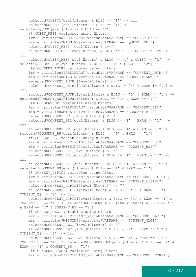
C - 217

selected$QUEST1[eval(filters) & ELIG != ’1’] <- irr selected$QUEST1[eval(filters) & ELIG == ’1’] <- selected$QUEST[eval(filters) & ELIG == ’1’] ## QUEST_REF1 variables using filters irr = variables$IRRELEVANT[variables$VARNAME == ”QUEST_REF1”] mis = variables$MISSING[variables$VARNAME == ”QUEST_REF1”] selected$QUEST_REF1[!eval(filters)] <- ”” selected$QUEST_REF1[eval(filters) & ELIG != ’1’ | QUEST != ”2”] <- irr selected$QUEST_REF1[eval(filters) & ELIG == ’1’ & QUEST == ”2”] <- selected$QUEST_REF[eval(filters) & ELIG == ’1’ & QUEST == ”2”] ## CONSENT_ANTR1 variables using filters irr = variables$IRRELEVANT[variables$VARNAME == ”CONSENT_ANTR1”] mis = variables$MISSING[variables$VARNAME == ”CONSENT_ANTR1”] selected$CONSENT_ANTR1[!eval(filters)] <- ”” selected$CONSENT_ANTR1[eval(filters) & ELIG != ’1’ | EXAM != ”1”] <- irr selected$CONSENT_ANTR1[eval(filters) & ELIG == ’1’ & EXAM == ”1”] <- selected$CONSENT_ANTR[eval(filters) & ELIG == ’1’ & EXAM == ”1”] ## CONSENT_BP1 variables using filters irr = variables$IRRELEVANT[variables$VARNAME == ”CONSENT_BP1”] mis = variables$MISSING[variables$VARNAME == ”CONSENT_BP1”] selected$CONSENT_BP1[!eval(filters)] <- ”” selected$CONSENT_BP1[eval(filters) & ELIG != ’1’ | EXAM != ”1”] <- irr selected$CONSENT_BP1[eval(filters) & ELIG == ’1’ & EXAM == ”1”] <- selected$CONSENT_BP[eval(filters) & ELIG == ’1’ & EXAM == ”1”] ## CONSENT_BS1 variables using filters irr = variables$IRRELEVANT[variables$VARNAME == ”CONSENT_BS1”] mis = variables$MISSING[variables$VARNAME == ”CONSENT_BS1”] selected$CONSENT_BS1[!eval(filters)] <- ”” selected$CONSENT_BS1[eval(filters) & ELIG != ’1’ | EXAM != ”1”] <- irr selected$CONSENT_BS1[eval(filters) & ELIG == ’1’ & EXAM == ”1”] <- selected$CONSENT_BS[eval(filters) & ELIG == ’1’ & EXAM == ”1”] ## CONSENT_LIPID1 variables using filters irr = variables$IRRELEVANT[variables$VARNAME == ”CONSENT_LIPID1”] mis = variables$MISSING[variables$VARNAME == ”CONSENT_LIPID1”] selected$CONSENT_LIPID1[!eval(filters)] <- ”” selected$CONSENT_LIPID1[eval(filters) & ELIG != ’1’ | EXAM != ”1” | CONSENT_BS != ”1”] <- irr selected$CONSENT_LIPID1[eval(filters) & ELIG == ’1’ & EXAM == ”1” & CONSENT_BS == ”1”] <- selected$CONSENT_LIPID[eval(filters) & ELIG == ’1’ & EXAM == ”1” & CONSENT_BS == ”1”] ## CONSENT_GLC1 variables using filters irr = variables$IRRELEVANT[variables$VARNAME == ”CONSENT_GLC1”] mis = variables$MISSING[variables$VARNAME == ”CONSENT_GLC1”] selected$CONSENT_GLC1[!eval(filters)] <- ”” selected$CONSENT_GLC1[eval(filters) & ELIG != ’1’ | EXAM != ”1” | CONSENT_BS != ”1”] <- irr selected$CONSENT_GLC1[eval(filters) & ELIG == ’1’ & EXAM == ”1” & CONSENT_BS == ”1”] <- selected$CONSENT_GLC[eval(filters) & ELIG == ’1’ & EXAM == ”1” & CONSENT_BS == ”1”] ## CONSENT_STORE1 variables using filters irr = variables$IRRELEVANT[variables$VARNAME == ”CONSENT_STORE1”]

C - 218

mis = variables$MISSING[variables$VARNAME == ”CONSENT_STORE1”] selected$CONSENT_STORE1[!eval(filters)] <- ”” selected$CONSENT_STORE1[eval(filters) & ELIG != ’1’ | EXAM != ”1” | CONSENT_BS != ”1”] <- irr selected$CONSENT_STORE1[eval(filters) & ELIG == ’1’ & EXAM == ”1” & CONSENT_BS == ”1”] <- selected$CONSENT_STORE[eval(filters) & ELIG == ’1’ & EXAM == ”1” & CONSENT_BS == ”1”] ## CONSENT_DNA1 variables using filters irr = variables$IRRELEVANT[variables$VARNAME == ”CONSENT_DNA1”] mis = variables$MISSING[variables$VARNAME == ”CONSENT_DNA1”] selected$CONSENT_DNA1[!eval(filters)] <- ”” selected$CONSENT_DNA1[eval(filters) & ELIG != ’1’ | EXAM != ”1” | CONSENT_BS != ”1”] <- irr selected$CONSENT_DNA1[eval(filters) & ELIG == ’1’ & EXAM == ”1” & CONSENT_BS == ”1”] <- selected$CONSENT_DNA[eval(filters) & ELIG == ’1’ & EXAM == ”1” & CONSENT_BS == ”1”] ## EXAMQUEST variables using filters irr = variables$IRRELEVANT[variables$VARNAME == ”EXAMQUEST”] mis = variables$MISSING[variables$VARNAME == ”EXAMQUEST”] selected$EXAMQUEST[!eval(filters)] <- ”” selected$EXAMQUEST[eval(filters) & ELIG != ’1’] <- irr selected$EXAMQUEST[eval(filters) & ELIG == ’1’ & EXAM == ”1” & QUEST == ”1”] <- ”1” selected$EXAMQUEST[eval(filters) & ELIG == ’1’ & (EXAM != ”1” | QUEST != ”1”)] <- ”2” detach(selected) selected <- try(selected[, c(’PID’, ’COUNTRY’, ’SURVEY’, ’SERIAL’, ’ELIG’, ’EXAM1’, ’REASON1’, ’EXAM_REF1’, ’EXAM_NOAPP1’, ’QUEST1’, ’QUEST_REF1’, ’CONSENT_ANTR1’,’CONSENT_BP1’,’CONSENT_BS1’,’CONSENT_LIPID1’,’CONSENT_GLC1’,’CONSENT_DNA1’,’CONSENT_STORE1’, ’EXAMQUEST’)] , TRUE) if (class( selected ) == ”try-error”) { stop(paste(’Selected variables not found from dataset.’, ’\n’, sep=””)) } if (!is.null(outdata) ) { outdata <- merge(outdata, selected, all=T) } if (is.null(outdata)) { outdata <- selected } selected <- NULL tstop <- Sys.time() cat(’EHES_derived_variables_elig function call completed in ’, format(round(difftime(tstop, tstart, units=’mins’), digits=3), nsmall=3), ’.’, ’\n\n’, sep=’’) return(outdata)}

derived_variables_schooling - to calculate third of years of education variable

derived_variables_schooling <- function(data=NA, variables) { ### data = dataset, variables = definition table for variables

C - 219

tstart <- Sys.time() outdata=NULL if (is.null(data) ) { stop(”\n***ERROR:***\n No data given. Execution halted.”) } cat(’Creating variables:\nSCHOOL_THIRDS’, ’\n\n’, sep=’’) selected <- try(data[, c(’PID’, ’COUNTRY’, ’SURVEY’, ’SERIAL’, ’EXAM’, ’QUEST’, ’BIRTH_YEAR’, ’SCHOOL_YEARS’, ’SEX’)] , TRUE) if (class( selected ) == ”try-error”) { stop(paste(’Selected variables not found from dataset \n’, sep=””)) } filters <- expression(EXAM == ’1’ | QUEST == ’1’) attach(selected) selected = selected[eval(filters),] detach(selected) irr = ”” mis = variables$MISSING[variables$VARNAME == ”SCHOOL_YEARS”] selected$SCHOOL_YEARS = code_miss_numeric(selected, ’SCHOOL_YEARS’, mis, irr, filter=filters ) ### removing missing observations selected1 <- selected[, c(”PID”, ”COUNTRY”, ”SURVEY”, ”SERIAL”, ”EXAM”, ”QUEST”)] selected = selected[!is.na(selected$SCHOOL_YEARS) & !is.na(selected$BIRTH_YEAR) ,] #Create key variables selected$GROUP<-paste(selected$COUNTRY, selected$SEX, sep=””) selected$GROUPY<-paste(selected$GROUP, selected$BIRTH_YEAR, sep=””) GROUPYS<-sort(unique(selected$GROUPY)) #Create data frame for cutpoints tert1<-data.frame(SERIAL=GROUPYS,GROUP=substr(GROUPYS,1,3),COUNTRY=substr(GROUPYS,1,2),SEX=substr(GROUPYS,3,3),YEAR=substr(GROUPYS,4,7)) tert1$YEAR<-as.numeric(levels(tert1$YEAR))[tert1$YEAR] #Add starting values tert2<-tert1 tert2$YEAR<-tert1$YEAR-3 tert2$SERIAL<-paste(tert2$GROUP,tert2$YEAR,sep=””) tert<-merge(tert1,tert2,all=TRUE) #The function which calculate tertiles tertiles<-function(var){ l<-quantile(var, probs=0.3333, type=1,na.rm=TRUE) u<-quantile(var, probs=0.6667, type=1,na.rm=TRUE) n<-length(var[!is.na(var)]) c1<-sum(var<l,na.rm=TRUE)/n c2<-sum(var==l,na.rm=TRUE)/n c3<-sum(var>l & var<u,na.rm=TRUE)/n c4<-sum(var==u,na.rm=TRUE)/n c5<-sum(var>u,na.rm=TRUE)/n return(c(l,u,c1,c2,c3,c4,c5)) } #Calculate tertiles for (i in 1:nrow(tert)) { group<-tert$GROUP[i] year<-tert$YEAR[i] x<-selected$SCHOOL_YEARS[selected$GROUP==group & abs(as.

C - 220

numeric(selected$BIRTH_YEAR)-year)<4] y<-tertiles(as.numeric(x)) y<-as.numeric(y) tert$L[i]<-y[1] tert$U[i]<-y[2] tert$C1[i]<-y[3] tert$C2[i]<-y[4] tert$C3[i]<-y[5] tert$C4[i]<-y[6] tert$C5[i]<-y[7] } #Define first year for (i in 1:nrow(tert)) { if (i==1) { tert$cond[i]<-1 } else if (tert$GROUP[i]!=tert$GROUP[i-1]) { tert$cond[i]<-1 } else { tert$cond[i]<-0 } } #Calculate cutpoints for (i in 1:nrow(tert)){ l<-tert$L[i] u<-tert$U[i] c1<-tert$C1[i] c2<-tert$C2[i] c3<-tert$C3[i] c4<-tert$C4[i] c5<-tert$C5[i] if (tert$cond[i]==1){ absdiff1<-abs(1/3-c1)+abs(1/3-c2-c3-c4)+abs(1/3-c5)+10*(c1<0.15)+10*(c5<0.15)+10*(c1<0.25)*(0.25-c1)+10*(c5<0.25)*(0.25-c5) absdiff<-absdiff1 LOW<-l-0.5 UP<-u+0.5 absdiff2<-abs(1/3-c1-c2)+abs(1/3-c3-c4)+abs(1/3-c5)+10*((c1+c2)<0.15)+10*(c5<0.15)+10*((c1+c2)<0.25)*(0.25-c1-c2)+10*(c5<0.25)*(0.25-c5)+10*(u==l) if (absdiff2<absdiff) { absdiff<-absdiff2 LOW<-l+0.5 UP<-u+0.5 } absdiff3<-abs(1/3-c1)+abs(1/3-c2-c3)+abs(1/3-c4-c5)+10*(c1<0.15)+10*((c4+c5)<0.15)+10*(c1<0.25)*(0.25-c1)+10*((c4+c5)<0.25)*(0.25-c4-c5)+10*(u==l) if (absdiff3<absdiff) { absdiff<-absdiff3 LOW<-l-0.5 UP<-u-0.5 } absdiff4=abs(1/3-c1-c2)+abs(1/3-c3)+abs(1/3-c4-c5)+

C - 221

10*((c1+c2)<0.15)+10*((c4+c5)<0.15)+10*((c1+c2)<0.25)*(0.25-c1-c2)+10*((c4+c5)<0.25)*(0.25-c4-c5)+10*((u-l)==1)+100*(u==l); if (absdiff4<absdiff) { absdiff<-absdiff4 LOW<-l+0.5 UP<-u-0.5 } } else { LOW1<-tert$LOW[i-1] UP1<-tert$UP[i-1] absdiff1<-abs(1/3-c1)+abs(1/3-c2-c3-c4)+abs(1/3-c5)+10*(c1<0.15)+10*(c5<0.15)+10*(c1<0.25)*(0.25-c1)+10*(c5<0.25)*(0.25-c5)+0.2*((l-0.5)!=LOW1)+0.2*((u+0.5)!=UP1) absdiff<-absdiff1 LOW<-l-0.5 UP<-u+0.5 absdiff2<-abs(1/3-c1-c2)+abs(1/3-c3-c4)+abs(1/3-c5)+10*((c1+c2)<0.15)+10*(c5<0.15)+10*((c1+c2)<0.25)*(0.25-c1-c2)+10*(c5<0.25)*(0.25-c5)+10*(u==l)+0.2*((l+0.5)!=LOW1)+0.2*((u+0.5)!=UP1) if (absdiff2<absdiff) { absdiff<-absdiff2 LOW<-l+0.5 UP<-u+0.5 } absdiff3<-abs(1/3-c1)+abs(1/3-c2-c3)+abs(1/3-c4-c5)+10*(c1<0.15)+10*((c4+c5)<0.15)+10*(c1<0.25)*(0.25-c1)+10*((c4+c5)<0.25)*(0.25-c4-c5)+10*(u==l)+0.2*((l-0.5)!=LOW1)+0.2*((u-0.5)!=UP1) if (absdiff3<absdiff) { absdiff<-absdiff3 LOW<-l-0.5 UP<-u-0.5 } absdiff4=abs(1/3-c1-c2)+abs(1/3-c3)+abs(1/3-c4-c5)+10*((c1+c2)<0.15)+10*((c4+c5)<0.15)+10*((c1+c2)<0.25)*(0.25-c1-c2)+10*((c4+c5)<0.25)*(0.25-c4-c5)+10*((u-l)==1)+100*(u==l)+0.2*((l+0.5)!=LOW1)+0.2*((u-0.5)!=UP1); if (absdiff4<absdiff) { absdiff<-absdiff4 LOW<-l+0.5 UP<-u-0.5 } } tert$LOW[i]<-LOW tert$UP[i]<-UP } #Drop starting values tert<-merge(tert,tert1,all.y=TRUE) selected<-merge(selected,tert[,c(”SERIAL”,”LOW”,”UP”)],by.x=”GROUPY”,by.y=”SERIAL”) selected <- selected[, c(’PID’, ’COUNTRY’, ’SURVEY’, ’SERIAL’, ’EXAM’, ’QUEST’, ’SCHOOL_YEARS’, ’LOW’, ’UP’)] selected<-merge(selected,selected1, all=T) #Classify data by cutpoints

C - 222

mis = variables$MISSING[variables$VARNAME == ”SCHOOL_THIRDS”] irr = variables$IRRELEVANT[variables$VARNAME == ”SCHOOL_THIRDS”] attach(selected) selected$SCHOOL_THIRDS <- irr selected$SCHOOL_THIRDS[eval(filters) & !is.na(selected$SCHOOL_YEARS)& selected$SCHOOL_YEARS<selected$LOW]<-’1’ selected$SCHOOL_THIRDS[eval(filters) & !is.na(selected$SCHOOL_YEARS)& selected$SCHOOL_YEARS<selected$UP & selected$SCHOOL_YEARS>selected$LOW]<-’2’ selected$SCHOOL_THIRDS[eval(filters) & !is.na(selected$SCHOOL_YEARS) & selected$SCHOOL_YEARS>selected$UP]<-’3’ selected$SCHOOL_THIRDS[eval(filters) & is.na(selected$SCHOOL_YEARS)]<-mis detach(selected) selected <- selected[, c(’PID’, ’COUNTRY’, ’SURVEY’, ’SERIAL’, ’EXAM’, ’QUEST’,’SCHOOL_THIRDS’)] if (!is.null(outdata) ) { outdata <- merge(outdata, selected, all=T) } if (is.null(outdata)) { outdata <- selected } selected <- NULL tstop <- Sys.time() cat(’EHES_derived_variables_schooling function call completed in ’, format(round(difftime(tstop, tstart, units=’mins’), digits=3), nsmall=3), ’.’, ’\n\n’, sep=’’) return(outdata)}

derived_variables_income - to calculate family income and household’s equivalised disposable income

derived_variables_income <- function(data=NA, variables, dlimits) { ### data = dataset, variables = definition table for variables tstart <- Sys.time() outdata=NULL if (is.null(data) ) { stop(”\n***ERROR:***\n No data given. Execution halted.”) } cat(’Creating variables: FINCOME, INCOME_CLASS.\n’, ’\n\n’, sep=’’) selected <- try(data[, c(’PID’, ’COUNTRY’, ’SURVEY’, ’SERIAL’, ’EXAM’, ’QUEST’, ’TOTAL_INCOME’, ’PERSONS’)] , TRUE) if (class( selected ) == ”try-error”) { stop(paste(’Selected variables not found from dataset \n’, sep=””)) } filters <- expression(EXAM == ’1’ | QUEST == ’1’) attach(selected) selected = selected[eval(filters),] detach(selected) irr = ”” mis1 = variables$MISSING[variables$VARNAME == ”PERSONS”] mis2 = variables$MISSING[variables$VARNAME == ”TOTAL_INCOME”] notknown2 = variables$DONTKNOW[variables$VARNAME == ”TOTAL_INCOME”]

C - 223

## converting to numeric selected$PERSONS = code_miss_numeric(selected, ’PERSONS’, mis1, irr, filter=filters ) selected$KEY<-paste(selected$COUNTRY,selected$SURVEY,sep=””) dlimits$KEY<-paste(dlimits$COUNTRY, dlimits$SURVEY,sep=””) dlimits$L1<-as.numeric(dlimits$L1) dlimits$L2<-as.numeric(dlimits$L2) dlimits$L3<-as.numeric(dlimits$L3) dlimits$L4<-as.numeric(dlimits$L4) dlimits$L5<-as.numeric(dlimits$L5) dlimits$L6<-as.numeric(dlimits$L6) dlimits$L7<-as.numeric(dlimits$L7) dlimits$L8<-as.numeric(dlimits$L8) dlimits$L9<-as.numeric(dlimits$L9) dlimits$NCLASS<-as.numeric(dlimits$NCLASS) for (j in 1:nrow(dlimits)) { selected1<-selected[selected$KEY==dlimits$KEY[j],] selected1<-selected1[selected1$TOTAL_INCOME!=mis2 & selected1$TOTAL_INCOME!=notknown2 & !is.na(selected1$TOTAL_INCOME) & selected1$TOTAL_INCOME!=irr & selected1$PERSONS>0 & !is.na(selected1$PERSONS),] if (nrow(selected1)>0) { nclass<-as.numeric(dlimits$NCLASS[j]) limits<-dlimits[j,4:(nclass+2)] limits<-as.numeric(limits) ######Define limits of income classes, weighting variable limits<-log(limits) selected1$CWEIGHT[1:nrow(selected1)]<-1 selected1$CWEIGHT<-as.numeric(selected1$CWEIGHT) ######Calculate class frequencies n<-sum(as.numeric(selected1$CWEIGHT)) frek<-c(1:nclass) for (i in 1:nclass) { frek[i]<-sum(selected1$CWEIGHT[selected1$TOTAL_INCOME==i])/n } ######A log-linear approximation for lowest and highest income classes p1<-frek[1] p10<-frek[nclass] z1<-qnorm(p1) z10<-qnorm(1-p10) x1<-as.numeric(limits[1]) x10<-as.numeric(limits[length(limits)]) sigma<-(x10-x1)/(z10-z1) mu<-x1-z1*sigma m1<-exp(mu+sigma*qnorm(p1/2)) m10<-exp(mu+sigma*qnorm(1-0.5*p10)) ######Calculate densities for limitspoin of lowest and highest income classes dens<-c(1:nclass) dens[1]<-dnorm(x1,mean=mu,sd=sigma) dens[nclass]<-dnorm(x10,mean=mu,sd=sigma) ######Calculate densities for midpoints of other classes for (i in 2:(nclass-1)) {

C - 224

dens[i]<-frek[i]/(limits[i]-limits[i-1]) } points<-c(1:nclass) points[1]<-limits[1] points[nclass]<-limits[nclass-1] for (i in 2:(nclass-1)) { points[i]<-0.5*(limits[i-1]+limits[i]) } #####A piecewise linear approximation of the density function alpha<-c(1:(nclass-2)) beta<-c(1:(nclass-2)) for (i in 1:(nclass-2)) { beta[i]<-(dens[i+2]-dens[i])/(points[i+2]-points[i]) if (abs(beta[i])>dens[i+1]/(points[i+1]-limits[i])) { beta[i]<-sign(dens[i+2]-dens[i])*dens[i+1]/(points[i+1]-limits[i]) } alpha[i]<-dens[i+1]-beta[i]*points[i+1] } ######Calculate median for each class mpoint<-c(1:nclass) mpoint[1]<-exp(mu+sigma*qnorm(p1/2)) mpoint[nclass]<-exp(mu+sigma*qnorm(1-0.5*p10)) for (i in 2:(nclass-1)) { a<-beta[i-1]/2 b<-alpha[i-1] c<--0.5*beta[i-1]*limits[i-1]^2-alpha[i-1]*limits[i-1]-0.5*frek[i] if (a==0) { mpoint[i]<-exp(points[i]) } else { mpoint[i]<-exp((-b+sqrt(b^2-4*a*c))/(2*a)) } } ######Calculate family income for (i in 1:nclass) { selected1$INCOME[selected1$TOTAL_INCOME==i]<-mpoint[i] } selected1$FINCOME<-selected1$INCOME/sqrt(as.numeric(selected1$PERSONS)) ######Calculate quantiles for the family income q<-quantile(selected1$FINCOME,probs=seq(0,1,0.2),na.rm=TRUE,names=FALSE,type=1,weigth=selected1$CWEIGHT) ######Initial grouping of the family income q[1]<-0 q[6]<-q[6]+1 for (i in 1:5) { selected1$CLASS[selected1$FINCOME>q[i] & selected1$FINCOME<q[i+1] & !is.na(selected1$FINCOME)]<-i ######Observations which equals a class limit selected1$CLASS[selected1$FINCOME==q[i+1]]<-i+0.5 } ######Classify limit observations

C - 225

n<-sum(selected1$CWEIGHT[!is.na(selected1$CLASS)]) selected1$CLASS<-as.numeric(selected1$CLASS) for (i in 1:4) { l<-0.2*i*n-sum(selected1$CWEIGHT[!is.na(selected1$CLASS) & selected1$CLASS<=i]) u<-sum(selected1$CWEIGHT[!is.na(selected1$CLASS) & selected1$CLASS<i+1])-0.2*i*n selected1$CLASS[!is.na(selected1$CLASS) & selected1$CLASS==i+0.5]<-selected1$CLASS[!is.na(selected1$CLASS) & selected1$CLASS==i+0.5]+sign(u-l)*0.5 } ######Classify remaining limit observations if (sum(!is.na(selected1$CLASS) & (selected1$CLASS-floor(selected1$CLASS)==0.5))>0) { for (i in 1:4) { if (sum(!is.na(selected1$CLASS) & selected1$CLASS==i+0.5)>0) { sum1<-sum(selected1$CWEIGHT[!is.na(selected1$CLASS) & selected1$CLASS==i]) sum2<-sum(selected1$CWEIGHT[!is.na(selected1$CLASS) & selected1$CLASS==i+1]) if (sum1<sum2) { selected1$CLASS[selected1$CLASS==i+0.5]<-i } else if (sum1<sum2) { selected1$CLASS[selected1$CLASS==i+0.5]<-i+1 } else if (i==1|i==2) { selected1$CLASS[selected1$CLASS==i+0.5]<-i } else { selected1$CLASS[selected1$CLASS==i+0.5]<-i+1 } } } } selected1$INCOME_CLASS<-selected1$CLASS selected1<-selected1[,c(’KEY’,’SERIAL’,’FINCOME’,’INCOME_CLASS’)] if (j==1) { incomes<-selected1 } if (j>1) { incomes<-merge(incomes,selected1,all=TRUE) } } selected1=NULL } selected<-merge(incomes,selected,all=TRUE) #Missing values mis1 = variables$MISSING[variables$VARNAME == ”FINCOME”] mis2 = variables$MISSING[variables$VARNAME == ”INCOME_CLASS”] attach(selected) ### rounding to integer selected$FINCOME[eval(filters)]<- format(round(selected[eval(filters)

C - 226

,c(’FINCOME’)] , 0), nsmall=0, trim=T) selected$FINCOME[eval(filters) & selected$FINCOME == ”NA”]<-mis1 selected$INCOME_CLASS[eval(filters) & is.na(selected$INCOME_CLASS)]<-mis2 detach(selected) selected <- selected[, c(’PID’, ’COUNTRY’, ’SURVEY’, ’SERIAL’, ’EXAM’, ’QUEST’,’FINCOME’, ’INCOME_CLASS’)] if (!is.null(outdata) ) { outdata <- merge(outdata, selected, all=T) } if (is.null(outdata)) { outdata <- selected } selected <- NULL tstop <- Sys.time() cat(’EHES_derived_variables_income function call completed in ’, format(round(difftime(tstop, tstart, units=’mins’), digits=3), nsmall=3), ’.’, ’\n\n’, sep=’’) return(outdata)}

Estimation of indicators

drawmeans - to calculate means, standard errors and 95 % confidence intervals for continuous varibles by survey, sex and 10-year age-groups and age-standardisation for 25-64-year-olds by sex

drawmeans <- function(data, varname, mis=NA, irr=NA, filters=TRUE) { ### data = dataset, varname = name of the variable, mis = code for missing value, irr = code for irrelevants, filters = indicators for participation data <- data[, c(”COUNTRY”, ”SURVEY”, ”EXAM”, ”QUEST”, ”SEX”, ”AGE”, varname)] attach(data) data = data[eval(filters),] detach(data) countries <- unique(data$COUNTRY) ns_header = c(”25-64_n_nonmissing”, ”men_25-64_n_nonmissing”, ”women_25-64_n_nonmissing”, ”men_25-64_nmissing”, ”women_25-64_nmissing”, ”men_25-34_n”, ”men_35-44_n”, ”men_45-54_n”, ”men_55-64_n”, ”men_25-34_mean”, ”men_35-44_mean”, ”men_45-54_mean”, ”men_55-64_mean”, ”men_25-64_mean”, ”men_25-34_se”, ”men_35-44_se”, ”men_45-54_se”, ”men_55-64_se”, ”men_25-64_se”, ”women_25-34_n”, ”women_35-44_n”, ”women_45-54_n”, ”women_55-64_n”, ”women_25-34_mean”, ”women_35-44_mean”, ”women_45-54_mean”, ”women_55-64_mean”, ”women_25-64_mean”, ”women_25-34_se”, ”women_35-44_se”, ”women_45-54_se”, ”women_55-64_se”, ”women_25-64_se” , ”men_25-34_cil”, ”men_35-44_cil”, ”men_45-54_cil”, ”men_55-64_cil”, ”men_25-64_cil”, ”men_25-34_ciu”, ”men_35-44_ciu”,

C - 227

”men_45-54_ciu”, ”men_55-64_ciu”, ”men_25-64_ciu”, ”women_25-34_cil”, ”women_35-44_cil”, ”women_45-54_cil”, ”women_55-64_cil”, ”women_25-64_cil”, ”women_25-34_ciu”, ”women_35-44_ciu”, ”women_45-54_ciu”, ”women_55-64_ciu”, ”women_25-64_ciu”) rows <- as.data.frame(cbind(””,””,”” , ””), stringsAsFactors = F ) names(rows) = c(”country”, ”survey”, ”ns_header”, ”ns”) firstrow=T for (country in countries) { surveys <- sort(unique(data[data$COUNTRY == country,]$SURVEY)) for (survey in surveys) { selected <- data[data$COUNTRY == country & data$SURVEY == survey & data$AGE >= 25 & data$AGE < 65, ] selected <- selected[ !(selected[, varname] %in% c(irr) ) & selected[, varname] != ” ” ,] nall1 <- nrow(selected) if (nall1 != 0) { nall1=NULL nall <- nrow(selected[!(selected[, varname] %in% c(mis) ), ]) nmen <- nrow(selected[!(selected[, varname] %in% c(mis) ) & selected$SEX == ”1”, ]) nwomen <- nrow(selected[!(selected[, varname] %in% c(mis) ) & selected$SEX == ”2”, ]) nmism <- nrow(selected[ selected[, varname] %in% mis & selected$SEX == ”1”,]) nmisw <- nrow(selected[ selected[, varname] %in% mis & selected$SEX == ”2”,]) if ( (nmism + nmisw) == nall) { mean11 = ””; mean12 = ””; mean21 = ””; mean22 = ””; mean31 = ””; mean32 = ””; mean41 = ””; mean42 = ””; mean1 = ””; mean2 = ”” n11 = ””; n12 = ””; n21 = ””; n22 = ””; n31 = ””; n32 = ””; n41 = ””; n42 = ””; n1 = ””; n2 = ”” se11 = ””; se12 = ””; se21 = ””; se22 = ””; se31 = ””; se32 = ””; se41 = ””; se42 = ””; se1 = ””; se2 = ”” cil11 = ””; cil12 = ””; cil21 = ””; cil22 = ””; cil31 = ””; cil32 = ””; cil41 = ””; cil42 = ””; cil1 = ””; cil2 = ”” ciu11 = ””; ciu12 = ””; ciu21 = ””; ciu22 = ””; ciu31 = ””; ciu32 = ””; ciu41 = ””; ciu42 = ””; ciu1 = ””; ciu2 = ”” }

else { selected[ selected[, varname] %in% c(mis,irr) , varname] <- ”” selected[, varname] <- as.numeric(selected[, varname]) age1 <- selected[selected$AGE >= 25 & selected$AGE < 35 , ] age2 <- selected[selected$AGE >= 35 & selected$AGE < 45 , ] age3 <- selected[selected$AGE >= 45 & selected$AGE < 55 , ] age4 <- selected[selected$AGE >= 55 & selected$AGE < 65 , ]

C - 228

if (nmen !=0 ) { mean11 <- mean(age1[age1$SEX == ”1”, varname], na.rm=T) mean21 <- mean(age2[age2$SEX == ”1”, varname], na.rm=T) mean31 <- mean(age3[age3$SEX == ”1”, varname], na.rm=T) mean41 <- mean(age4[age4$SEX == ”1”, varname], na.rm=T) n11 <- length(na.omit(age1[age1$SEX == ”1”, varname])) n21 <- length(na.omit(age2[age2$SEX == ”1”, varname])) n31 <- length(na.omit(age3[age3$SEX == ”1”, varname])) n41 <- length(na.omit(age4[age4$SEX == ”1”, varname])) se11 <- sqrt(var(age1[age1$SEX == ”1”, varname], na.rm=T) / n11) se21 <- sqrt(var(age2[age2$SEX == ”1”, varname], na.rm=T) / n21) se31 <- sqrt(var(age3[age3$SEX == ”1”, varname], na.rm=T) / n31) se41 <- sqrt(var(age4[age4$SEX == ”1”, varname], na.rm=T) / n41) se1 <- sqrt( sum( ((1/length(c(se11, se21, se31, se41)) ) * c(se11, se21, se31, se41))^2 )) mean1 <- mean(c(mean11, mean21, mean31, mean41)) cil11 <- mean11 - 1.96*se11 cil21 <- mean21 - 1.96*se21 cil31 <- mean31 - 1.96*se31 cil41 <- mean41 - 1.96*se41 cil1 <- mean1 - 1.96*se1 ciu11 <- mean11 + 1.96*se11 ciu21 <- mean21 + 1.96*se21 ciu31 <- mean31 + 1.96*se31 ciu41 <- mean41 + 1.96*se41 ciu1 <- mean1 + 1.96*se1 se1 = format(round(se1, 3 ), nsmall=3) mean1 = format(round(mean1, 2), nsmall=2) mean11 = format(round(mean11, 2), nsmall=2) mean21 = format(round(mean21, 2), nsmall=2) mean31 = format(round(mean31, 2), nsmall=2) mean41 = format(round(mean41, 2), nsmall=2) se11 = format(round(se11, 3), nsmall=3) se21 = format(round(se21, 3), nsmall=3) se31 = format(round(se31, 3), nsmall=3) se41 = format(round(se41, 3), nsmall=3) cil11 = format(round(cil11, 1), nsmall=1) cil21 = format(round(cil21, 1), nsmall=1) cil31 = format(round(cil31, 1), nsmall=1) cil41 = format(round(cil41, 1), nsmall=1) cil1 = format(round(cil1, 1), nsmall=1) ciu11 = format(round(ciu11, 1), nsmall=1) ciu21 = format(round(ciu21, 1), nsmall=1)

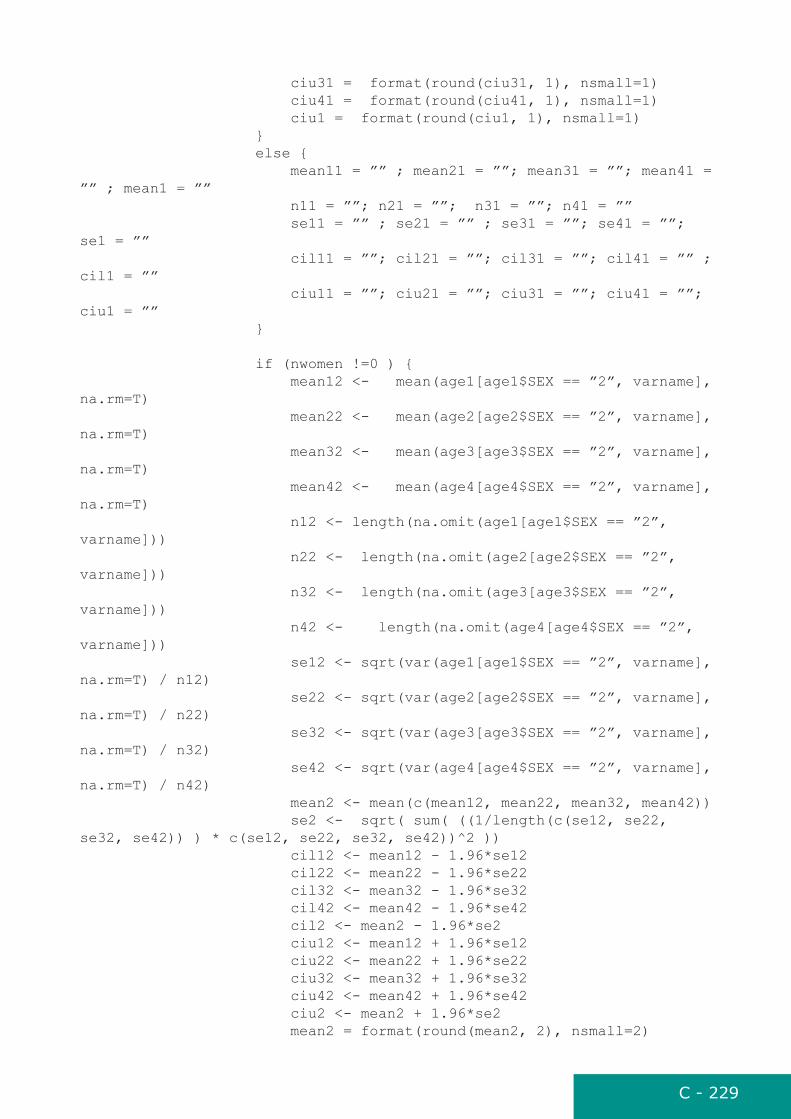
C - 229

ciu31 = format(round(ciu31, 1), nsmall=1) ciu41 = format(round(ciu41, 1), nsmall=1) ciu1 = format(round(ciu1, 1), nsmall=1) } else { mean11 = ”” ; mean21 = ””; mean31 = ””; mean41 = ”” ; mean1 = ”” n11 = ””; n21 = ””; n31 = ””; n41 = ”” se11 = ”” ; se21 = ”” ; se31 = ””; se41 = ””; se1 = ”” cil11 = ””; cil21 = ””; cil31 = ””; cil41 = ”” ; cil1 = ”” ciu11 = ””; ciu21 = ””; ciu31 = ””; ciu41 = ””; ciu1 = ”” }

if (nwomen !=0 ) { mean12 <- mean(age1[age1$SEX == ”2”, varname], na.rm=T) mean22 <- mean(age2[age2$SEX == ”2”, varname], na.rm=T) mean32 <- mean(age3[age3$SEX == ”2”, varname], na.rm=T) mean42 <- mean(age4[age4$SEX == ”2”, varname], na.rm=T) n12 <- length(na.omit(age1[age1$SEX == ”2”, varname])) n22 <- length(na.omit(age2[age2$SEX == ”2”, varname])) n32 <- length(na.omit(age3[age3$SEX == ”2”, varname])) n42 <- length(na.omit(age4[age4$SEX == ”2”, varname])) se12 <- sqrt(var(age1[age1$SEX == ”2”, varname], na.rm=T) / n12) se22 <- sqrt(var(age2[age2$SEX == ”2”, varname], na.rm=T) / n22) se32 <- sqrt(var(age3[age3$SEX == ”2”, varname], na.rm=T) / n32) se42 <- sqrt(var(age4[age4$SEX == ”2”, varname], na.rm=T) / n42) mean2 <- mean(c(mean12, mean22, mean32, mean42)) se2 <- sqrt( sum( ((1/length(c(se12, se22, se32, se42)) ) * c(se12, se22, se32, se42))^2 )) cil12 <- mean12 - 1.96*se12 cil22 <- mean22 - 1.96*se22 cil32 <- mean32 - 1.96*se32 cil42 <- mean42 - 1.96*se42 cil2 <- mean2 - 1.96*se2 ciu12 <- mean12 + 1.96*se12 ciu22 <- mean22 + 1.96*se22 ciu32 <- mean32 + 1.96*se32 ciu42 <- mean42 + 1.96*se42 ciu2 <- mean2 + 1.96*se2 mean2 = format(round(mean2, 2), nsmall=2)

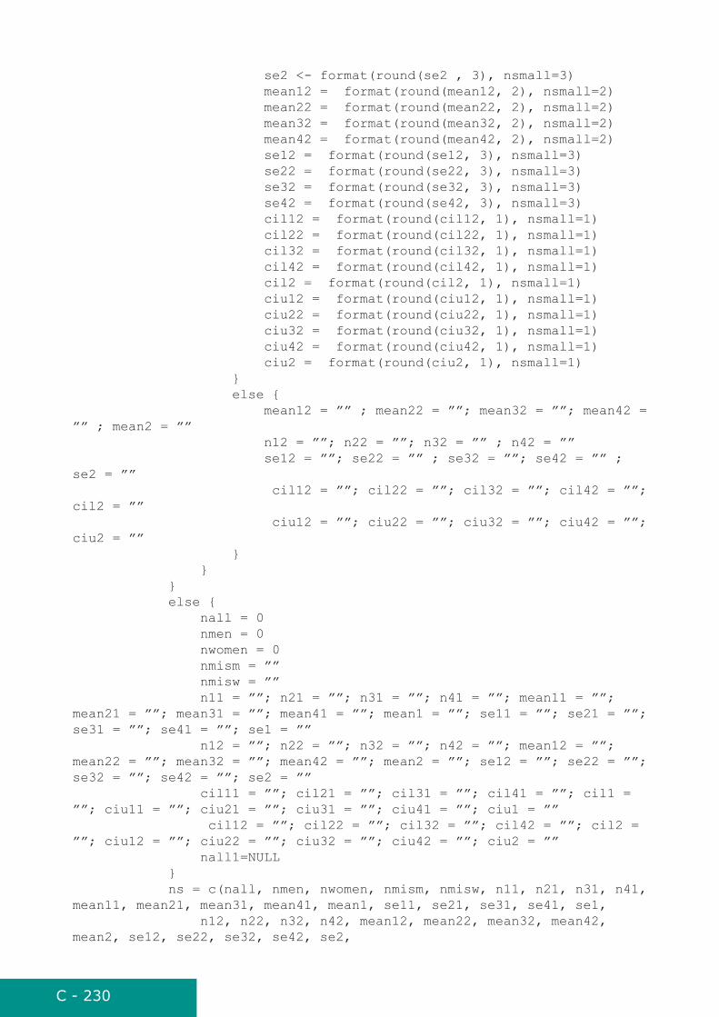
C - 230

se2 <- format(round(se2 , 3), nsmall=3) mean12 = format(round(mean12, 2), nsmall=2) mean22 = format(round(mean22, 2), nsmall=2) mean32 = format(round(mean32, 2), nsmall=2) mean42 = format(round(mean42, 2), nsmall=2) se12 = format(round(se12, 3), nsmall=3) se22 = format(round(se22, 3), nsmall=3) se32 = format(round(se32, 3), nsmall=3) se42 = format(round(se42, 3), nsmall=3) cil12 = format(round(cil12, 1), nsmall=1) cil22 = format(round(cil22, 1), nsmall=1) cil32 = format(round(cil32, 1), nsmall=1) cil42 = format(round(cil42, 1), nsmall=1) cil2 = format(round(cil2, 1), nsmall=1) ciu12 = format(round(ciu12, 1), nsmall=1) ciu22 = format(round(ciu22, 1), nsmall=1) ciu32 = format(round(ciu32, 1), nsmall=1) ciu42 = format(round(ciu42, 1), nsmall=1) ciu2 = format(round(ciu2, 1), nsmall=1) } else { mean12 = ”” ; mean22 = ””; mean32 = ””; mean42 = ”” ; mean2 = ”” n12 = ””; n22 = ””; n32 = ”” ; n42 = ”” se12 = ””; se22 = ”” ; se32 = ””; se42 = ”” ; se2 = ”” cil12 = ””; cil22 = ””; cil32 = ””; cil42 = ””; cil2 = ”” ciu12 = ””; ciu22 = ””; ciu32 = ””; ciu42 = ””; ciu2 = ”” } } } else { nall = 0 nmen = 0 nwomen = 0 nmism = ”” nmisw = ”” n11 = ””; n21 = ””; n31 = ””; n41 = ””; mean11 = ””; mean21 = ””; mean31 = ””; mean41 = ””; mean1 = ””; se11 = ””; se21 = ””; se31 = ””; se41 = ””; se1 = ”” n12 = ””; n22 = ””; n32 = ””; n42 = ””; mean12 = ””; mean22 = ””; mean32 = ””; mean42 = ””; mean2 = ””; se12 = ””; se22 = ””; se32 = ””; se42 = ””; se2 = ”” cil11 = ””; cil21 = ””; cil31 = ””; cil41 = ””; cil1 = ””; ciu11 = ””; ciu21 = ””; ciu31 = ””; ciu41 = ””; ciu1 = ”” cil12 = ””; cil22 = ””; cil32 = ””; cil42 = ””; cil2 = ””; ciu12 = ””; ciu22 = ””; ciu32 = ””; ciu42 = ””; ciu2 = ”” nall1=NULL } ns = c(nall, nmen, nwomen, nmism, nmisw, n11, n21, n31, n41, mean11, mean21, mean31, mean41, mean1, se11, se21, se31, se41, se1, n12, n22, n32, n42, mean12, mean22, mean32, mean42, mean2, se12, se22, se32, se42, se2,

C - 231

cil11, cil21, cil31, cil41, cil1, ciu11, ciu21, ciu31, ciu41, ciu1, cil12, cil22, cil32, cil42, cil2, ciu12, ciu22, ciu32, ciu42, ciu2) rows1 = cbind(country, survey, ns_header, ns) rows = rbind(rows, rows1) if (firstrow) { rows = rows[-c(1),] firstrow=F } } } ### TOTAL line country = ”ALL” survey = ”ALL” selected <- data[data$AGE >= 25 & data$AGE < 65, ] selected <- selected[ !(selected[, varname] %in% c(irr) ) & selected[, varname] != ” ” ,] nall1 <- nrow(selected) if (nall1 != 0) { nall <- nrow(selected[!(selected[, varname] %in% c(mis) ), ]) nmen <- nrow(selected[!(selected[, varname] %in% c(mis) ) & selected$SEX == ”1”, ]) nwomen <- nrow(selected[!(selected[, varname] %in% c(mis) ) & selected$SEX == ”2”, ]) nmism <- nrow(selected[ selected[, varname] %in% mis & selected$SEX == ”1”,]) nmisw <- nrow(selected[ selected[, varname] %in% mis & selected$SEX == ”2”,]) if (( nmism + nmisw) == nall) { mean11 = ””; mean12 = ””; mean21 = ””; mean22 = ””; mean31 = ””; mean32 = ””; mean41 = ””; mean42 = ””; mean1 = ””; mean2 = ”” n11 = ””; n12 = ””; n21 = ””; n22 = ””; n31 = ””; n32 = ””; n41 = ””; n42 = ””; n1 = ””; n2 = ”” se11 = ””; se12 = ””; se21 = ””; se22 = ””; se31 = ””; se32 = ””; se41 = ””; se42 = ””; se1 = ””; se2 = ”” cil11 = ””; cil12 = ””; cil21 = ””; cil22 = ””; cil31 = ””; cil32 = ””; cil41 = ””; cil42 = ””; cil1 = ””; cil2 = ”” ciu11 = ””; ciu12 = ””; ciu21 = ””; ciu22 = ””; ciu31 = ””; ciu32 = ””; ciu41 = ””; ciu42 = ””; ciu1 = ””; ciu2 = ”” } else { selected[ selected[, varname] %in% c(mis,irr) , varname] <- ”” selected[, varname] <- as.numeric(selected[, varname]) age1 <- selected[selected$AGE >= 25 & selected$AGE < 35 , ] age2 <- selected[selected$AGE >= 35 & selected$AGE < 45 , ] age3 <- selected[selected$AGE >= 45 & selected$AGE < 55 , ] age4 <- selected[selected$AGE >= 55 & selected$AGE < 65 , ] if (nmen !=0 ) { mean11 <- mean(age1[age1$SEX == ”1”, varname], na.rm=T) mean21 <- mean(age2[age2$SEX == ”1”, varname], na.rm=T) mean31 <- mean(age3[age3$SEX == ”1”, varname], na.rm=T) mean41 <- mean(age4[age4$SEX == ”1”, varname], na.rm=T) n11 <- length(na.omit(age1[age1$SEX == ”1”, varname]))

C - 232

n21 <- length(na.omit(age2[age2$SEX == ”1”, varname])) n31 <- length(na.omit(age3[age3$SEX == ”1”, varname])) n41 <- length(na.omit(age4[age4$SEX == ”1”, varname])) se11 <- sqrt(var(age1[age1$SEX == ”1”, varname], na.rm=T) / n11) se21 <- sqrt(var(age2[age2$SEX == ”1”, varname], na.rm=T) / n21) se31 <- sqrt(var(age3[age3$SEX == ”1”, varname], na.rm=T) / n31) se41 <- sqrt(var(age4[age4$SEX == ”1”, varname], na.rm=T) / n41) se1 <- sqrt( sum( ((1/length(c(se11, se21, se31, se41)) ) * c(se11, se21, se31, se41))^2 )) mean1 <- mean(c(mean11, mean21, mean31, mean41)) cil11 <- mean11 - 1.96*se11 cil21 <- mean21 - 1.96*se21 cil31 <- mean31 - 1.96*se31 cil41 <- mean41 - 1.96*se41 cil1 <- mean1 - 1.96*se1 ciu11 <- mean11 + 1.96*se11 ciu21 <- mean21 + 1.96*se21 ciu31 <- mean31 + 1.96*se31 ciu41 <- mean41 + 1.96*se41 ciu1 <- mean1 + 1.96*se1 se1 = format(round(se1, 3 ), nsmall=3) mean1 = format(round(mean1, 2), nsmall=2) mean11 = format(round(mean11, 2), nsmall=2) mean21 = format(round(mean21, 2), nsmall=2) mean31 = format(round(mean31, 2), nsmall=2) mean41 = format(round(mean41, 2), nsmall=2) se11 = format(round(se11, 3), nsmall=3) se21 = format(round(se21, 3), nsmall=3) se31 = format(round(se31, 3), nsmall=3) se41 = format(round(se41, 3), nsmall=3) cil11 = format(round(cil11, 1), nsmall=1) cil21 = format(round(cil21, 1), nsmall=1) cil31 = format(round(cil31, 1), nsmall=1) cil41 = format(round(cil41, 1), nsmall=1) cil1 = format(round(cil1, 1), nsmall=1) ciu11 = format(round(ciu11, 1), nsmall=1) ciu21 = format(round(ciu21, 1), nsmall=1) ciu31 = format(round(ciu31, 1), nsmall=1) ciu41 = format(round(ciu41, 1), nsmall=1) ciu1 = format(round(ciu1, 1), nsmall=1) } else { mean11 = ”” ; mean21 = ””; mean31 = ””; mean41 = ”” ; mean1 = ”” n11 = ””; n21 = ””; n31 = ””; n41 = ”” se11 = ”” ; se21 = ”” ; se31 = ””; se41 = ””; se1 = ”” cil11 = ””; cil21 = ””; cil31 = ””; cil41 = ”” ; cil1 = ”” ciu11 = ””; ciu21 = ””; ciu31 = ””; ciu41 = ””; ciu1 = ”” }

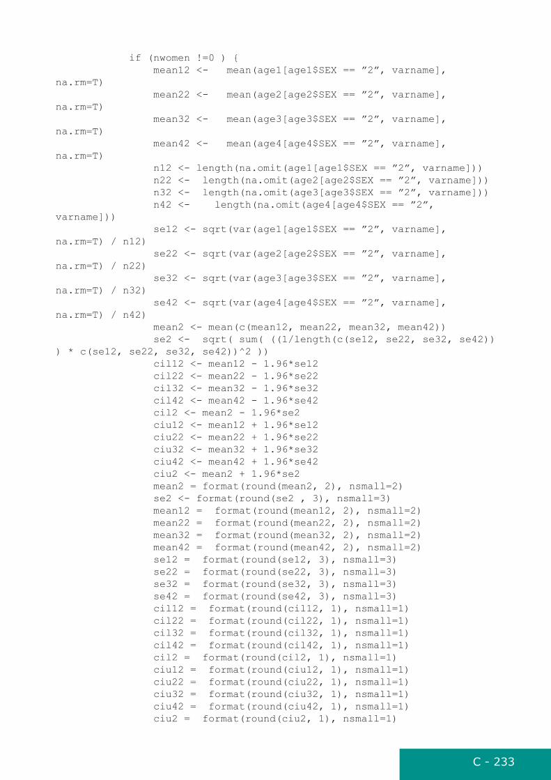
C - 233

if (nwomen !=0 ) { mean12 <- mean(age1[age1$SEX == ”2”, varname], na.rm=T) mean22 <- mean(age2[age2$SEX == ”2”, varname], na.rm=T) mean32 <- mean(age3[age3$SEX == ”2”, varname], na.rm=T) mean42 <- mean(age4[age4$SEX == ”2”, varname], na.rm=T) n12 <- length(na.omit(age1[age1$SEX == ”2”, varname])) n22 <- length(na.omit(age2[age2$SEX == ”2”, varname])) n32 <- length(na.omit(age3[age3$SEX == ”2”, varname])) n42 <- length(na.omit(age4[age4$SEX == ”2”, varname])) se12 <- sqrt(var(age1[age1$SEX == ”2”, varname], na.rm=T) / n12) se22 <- sqrt(var(age2[age2$SEX == ”2”, varname], na.rm=T) / n22) se32 <- sqrt(var(age3[age3$SEX == ”2”, varname], na.rm=T) / n32) se42 <- sqrt(var(age4[age4$SEX == ”2”, varname], na.rm=T) / n42) mean2 <- mean(c(mean12, mean22, mean32, mean42)) se2 <- sqrt( sum( ((1/length(c(se12, se22, se32, se42)) ) * c(se12, se22, se32, se42))^2 )) cil12 <- mean12 - 1.96*se12 cil22 <- mean22 - 1.96*se22 cil32 <- mean32 - 1.96*se32 cil42 <- mean42 - 1.96*se42 cil2 <- mean2 - 1.96*se2 ciu12 <- mean12 + 1.96*se12 ciu22 <- mean22 + 1.96*se22 ciu32 <- mean32 + 1.96*se32 ciu42 <- mean42 + 1.96*se42 ciu2 <- mean2 + 1.96*se2 mean2 = format(round(mean2, 2), nsmall=2) se2 <- format(round(se2 , 3), nsmall=3) mean12 = format(round(mean12, 2), nsmall=2) mean22 = format(round(mean22, 2), nsmall=2) mean32 = format(round(mean32, 2), nsmall=2) mean42 = format(round(mean42, 2), nsmall=2) se12 = format(round(se12, 3), nsmall=3) se22 = format(round(se22, 3), nsmall=3) se32 = format(round(se32, 3), nsmall=3) se42 = format(round(se42, 3), nsmall=3) cil12 = format(round(cil12, 1), nsmall=1) cil22 = format(round(cil22, 1), nsmall=1) cil32 = format(round(cil32, 1), nsmall=1) cil42 = format(round(cil42, 1), nsmall=1) cil2 = format(round(cil2, 1), nsmall=1) ciu12 = format(round(ciu12, 1), nsmall=1) ciu22 = format(round(ciu22, 1), nsmall=1) ciu32 = format(round(ciu32, 1), nsmall=1) ciu42 = format(round(ciu42, 1), nsmall=1) ciu2 = format(round(ciu2, 1), nsmall=1)

C - 234

} else { mean12 = ”” ; mean22 = ””; mean32 = ””; mean42 = ”” ; mean2 = ”” n12 = ””; n22 = ””; n32 = ”” ; n42 = ”” se12 = ””; se22 = ”” ; se32 = ””; se42 = ”” ; se2 = ”” cil12 = ””; cil22 = ””; cil32 = ””; cil42 = ””; cil2 = ”” ciu12 = ””; ciu22 = ””; ciu32 = ””; ciu42 = ””; ciu2 = ”” } } } else { nall = 0 nmen = 0 nwomen = 0 nmism = ”” nmisw = ”” n11 = ””; n21 = ””; n31 = ””; n41 = ””; mean11 = ””; mean21 = ””; mean31 = ””; mean41 = ””; mean1 = ””; se11 = ””; se21 = ””; se31 = ””; se41 = ””; se1 = ”” n12 = ””; n22 = ””; n32 = ””; n42 = ””; mean12 = ””; mean22 = ””; mean32 = ””; mean42 = ””; mean2 = ””; se12 = ””; se22 = ””; se32 = ””; se42 = ””; se2 = ”” cil21 = ””; cil31 = ””; cil41 = ””; cil1 = ””; ciu21 = ””; ciu31 = ””; ciu41 = ””; ciu1 = ”” cil12 = ””; cil22 = ””; cil32 = ””; cil42 = ””; cil2 = ”” ; ciu12 = ””; ciu22 = ””; ciu32 = ””; ciu42 = ””; ciu2 = ”” } ns = c(nall, nmen, nwomen, nmism, nmisw, n11, n21, n31, n41, mean11, mean21, mean31, mean41, mean1, se11, se21, se31, se41, se1, n12, n22, n32, n42, mean12, mean22, mean32, mean42, mean2, se12, se22, se32, se42, se2, cil11, cil21, cil31, cil41, cil1, ciu11, ciu21, ciu31, ciu41, ciu1, cil12, cil22, cil32, cil42, cil2, ciu12, ciu22, ciu32, ciu42, ciu2) rows1 = cbind(country, survey, ns_header, ns) rows = rbind(rows, rows1) cat(’Means for ’, varname, ’ done.\n’, sep=’’) return(rows)}

drawprops - to calculate proportions and number of observations for categor-ical varibles by survey, sex and 10-year age-groups and age-standardisation for 25-64-year-olds by sex

drawprops <- function(data, varname, mis=NA, irr=NA, filters=TRUE) { ### data = dataset, varname= name of the variable, mis = code for missing value, irr = code for irrelevants, filters = indicators for participation if (varname == ”ELIG” | varname == ”EXAM1” | varname == ”QUEST1” | varname == ”EXAMQUEST”) { data <- data[, c(”COUNTRY”, ”SURVEY”, ”SEX”, ”AGE”, varname)]

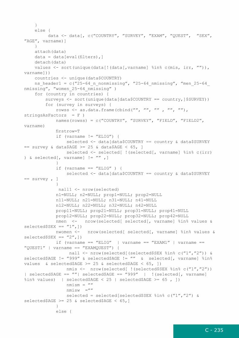
C - 235

} else { data <- data[, c(”COUNTRY”, ”SURVEY”, ”EXAM”, ”QUEST”, ”SEX”, ”AGE”, varname)] } attach(data) data = data[eval(filters),] detach(data) values <- sort(unique(data[!(data[,varname] %in% c(mis, irr, ””)), varname])) countries <- unique(data$COUNTRY) ns_header1 = c(”25-64_n_nonmissing”, ”25-64_nmissing”, ”men_25-64_nmissing”, ”women_25-64_nmissing” ) for (country in countries) { surveys <- sort(unique(data[data$COUNTRY == country,]$SURVEY)) for (survey in surveys) { rowss <- as.data.frame(cbind(””, ””, ”” , ””, ””), stringsAsFactors = F ) names(rowss) = c(”COUNTRY”, ”SURVEY”, ”FIELD”, ”FIELD2”, varname) firstrow=T if (varname != ”ELIG”) { selected <- data[data$COUNTRY == country & data$SURVEY == survey & data$AGE >= 25 & data$AGE < 65, ] selected <- selected[ !(selected[, varname] %in% c(irr) ) & selected[, varname] != ”” ,] } if (varname == ”ELIG” ) { selected <- data[data$COUNTRY == country & data$SURVEY == survey , ] } nall1 <- nrow(selected) n1=NULL; n2=NULL; prop1=NULL; prop2=NULL n11=NULL; n21=NULL; n31=NULL; n41=NULL n12=NULL; n22=NULL; n32=NULL; n42=NULL prop11=NULL; prop21=NULL; prop31=NULL; prop41=NULL prop12=NULL; prop22=NULL; prop32=NULL; prop42=NULL nmen <- nrow(selected[ selected[, varname] %in% values & selected$SEX == ”1”,]) nwomen <- nrow(selected[ selected[, varname] %in% values & selected$SEX == ”2”,]) if (varname == ”ELIG” | varname == ”EXAM1” | varname == ”QUEST1” | varname == ”EXAMQUEST”) { nall <- nrow(selected[(selected$SEX %in% c(”1”,”2”)) & selected$AGE != ”999” & selected$AGE != ”” & selected[, varname] %in% values & selected$AGE >= 25 & selected$AGE < 65, ]) nmis <- nrow(selected[ !(selected$SEX %in% c(”1”,”2”)) | selected$AGE == ””| selected$AGE == ”999” | !(selected[, varname] %in% values) | selected$AGE < 25 | selected$AGE >= 65 , ]) nmism = ”” nmisw =”” selected = selected[selected$SEX %in% c(”1”,”2”) & selected$AGE >= 25 & selected$AGE < 65,] } else {

C - 236

nall <- nrow(selected[!(selected[, varname] %in% c(mis) ), ]) nmis <- nrow(selected[ selected[, varname] %in% mis ,]) nmism <- nrow(selected[ selected[, varname] %in% mis & selected$SEX == ”1”,]) nmisw <- nrow(selected[ selected[, varname] %in% mis & selected$SEX == ”2”,]) } ### converting to numeric, missing values selected = selected[ !(selected[, varname] %in% c(mis)) , ] selected[, varname] <- as.numeric(selected[, varname]) age1 <- selected[selected$AGE >= 25 & selected$AGE < 35 , ] age2 <- selected[selected$AGE >= 35 & selected$AGE < 45 , ] age3 <- selected[selected$AGE >= 45 & selected$AGE < 55 , ] age4 <- selected[selected$AGE >= 55 & selected$AGE < 65 , ] if (nmen !=0 ) { n1[”all”] <- length(na.omit(selected[selected$SEX == ”1”, varname])) n11[”all”] <- length(na.omit(age1[age1$SEX == ”1”, varname])) n21[”all”] <- length(na.omit(age2[age2$SEX == ”1”, varname])) n31[”all”] <- length(na.omit(age3[age3$SEX == ”1”, varname])) n41[”all”] <- length(na.omit(age4[age4$SEX == ”1”, varname])) } if (nwomen !=0 ) { n2[”all”] <- length(na.omit(selected[selected$SEX == ”2”, varname])) n12[”all”] <- length(na.omit(age1[age1$SEX == ”2”, varname])) n22[”all”] <- length(na.omit(age2[age2$SEX == ”2”, varname])) n32[”all”] <- length(na.omit(age3[age3$SEX == ”2”, varname])) n42[”all”] <- length(na.omit(age4[age4$SEX == ”2”, varname])) } ns1 = c(nall, nmis, nmism, nmisw) rows1 = as.data.frame(cbind(country, survey, ns_header1, ”all”, ns1) , stringsAsFactors=F) names(rows1) <- c(”COUNTRY”, ”SURVEY”, ”FIELD”, ”FIELD2”, varname) ns1=NULL rowss = merge(rowss,rows1, all=T) if (nall!=0) { for (value in values) { if ( nall == 0) { n1[value] <- ””; n2[value] <- ”” n11[value] <- ””; n21[value] <- ””; n31[value] <- ””; n41[value] <- ””; n12[value] <- ””; n22[value] <- ””; n32[value] <- ””; n42[value] <- ”” prop1[value] <- ””; prop2[value] <- ””; prop11[value] <- ””; prop21[value] <- ””; prop31[value] <- ””;

C - 237

prop41[value] <- ”” prop12[value] <- ””; prop22[value] <- ””; prop32[value] <- ””; prop42[value] <- ”” } else { if (nmen !=0 ) { n1[value] <- length(na.omit(selected[selected$SEX == ”1” & selected[,varname] == value, varname])) n11[value] <- length(na.omit(age1[age1$SEX == ”1” & age1[,varname] == value, varname])) n21[value] <- length(na.omit(age2[age2$SEX == ”1” & age2[,varname] == value, varname])) n31[value] <- length(na.omit(age3[age3$SEX == ”1” & age3[,varname] == value, varname])) n41[value] <- length(na.omit(age4[age4$SEX == ”1” & age4[,varname] == value, varname])) prop11[value] <- 100*(n11[value] / n11[”all”]) prop21[value] <- 100*(n21[value] / n21[”all”] ) prop31[value] <- 100*(n31[value] / n31[”all”] ) prop41[value] <- 100*(n41[value] / n41[”all”] ) prop1[value] <- mean(c(prop11[value], prop21[value], prop31[value], prop41[value])) prop1[value] = format(round(as.numeric(prop1[value]), 1), nsmall=1) } else { prop1[value] = ”” prop11[value] = ”” prop21[value] = ”” prop31[value] = ”” prop41[value] = ”” n1[value] = ”0” n11[value] = ”0” n21[value] = ”0” n31[value] = ”0” n41[value] = ”0” } if (nwomen !=0 ) { n2[value] <- length(na.omit(selected[selected$SEX == ”2” & selected[,varname] == value, varname])) n12[value] <- length(na.omit(age1[age1$SEX == ”2” & age1[,varname] == value, varname])) n22[value] <- length(na.omit(age2[age2$SEX == ”2” & age2[,varname] == value, varname])) n32[value] <- length(na.omit(age3[age3$SEX == ”2” & age3[,varname] == value, varname])) n42[value] <- length(na.omit(age4[age4$SEX == ”2” & age4[,varname] == value, varname])) prop12[value] <- 100*(n12[value] /

C - 238

n12[”all”]) prop22[value] <- 100*(n22[value] / n22[”all”] ) prop32[value] <- 100*(n32[value] / n32[”all”] ) prop42[value] <- 100*(n42[value] / n42[”all”] ) prop2[value] <- mean(c(prop12[value], prop22[value], prop32[value], prop42[value])) prop2[value] = format(round(as.numeric(prop2[value]), 1), nsmall=1) } else { prop2[value] = ”” prop12[value] = ”” prop22[value] = ”” prop32[value] = ”” prop42[value] = ”” n2[value] = ”0” n12[value] = ”0” n22[value] = ”0” n32[value] = ”0” n42[value] = ”0” } } } ns2 = rbind( cbind(”men_25-34_n”,n11), cbind(”men_35-44_n”,n21), cbind(”men_45-54_n”,n31), cbind(”men_55-64_n”,n41), cbind(”men_25-64_n”,n1)) ns2 = cbind(rownames(ns2), ns2) rownames(ns2) <-NULL rows2 = as.data.frame(cbind(country, survey, ns2) , stringsAsFactors=F) names(rows2) <- c(”COUNTRY”, ”SURVEY”, ”FIELD2”, ”FIELD”, varname) ns2=NULL ns3 = rbind( cbind(”women_25-34_n”,n12), cbind(”women_35-44_n”,n22), cbind(”women_45-54_n”,n32), cbind(”women_55-64_n”,n42), cbind(”women_25-64_n”,n2)) ns3 = cbind(rownames(ns3), ns3) rownames(ns3) <-NULL rows3 = as.data.frame(cbind(country, survey, ns3) , stringsAsFactors=F) names(rows3) <- c(”COUNTRY”, ”SURVEY”, ”FIELD2”, ”FIELD”, varname) ns3=NULL ns4 = rbind( cbind(”men_25-34_percent”,prop11), cbind(”men_35-44_percent”,prop21), cbind(”men_45-54_percent”,prop31), cbind(”men_55-64_percent”,prop41), cbind(”men_25-64_percent”,prop1)) ns4 = cbind(rownames(ns4), ns4) rownames(ns4) <-NULL rows4 = as.data.frame(cbind(country, survey, ns4) , stringsAsFactors=F) names(rows4) <- c(”COUNTRY”, ”SURVEY”, ”FIELD2”, ”FIELD”, varname)

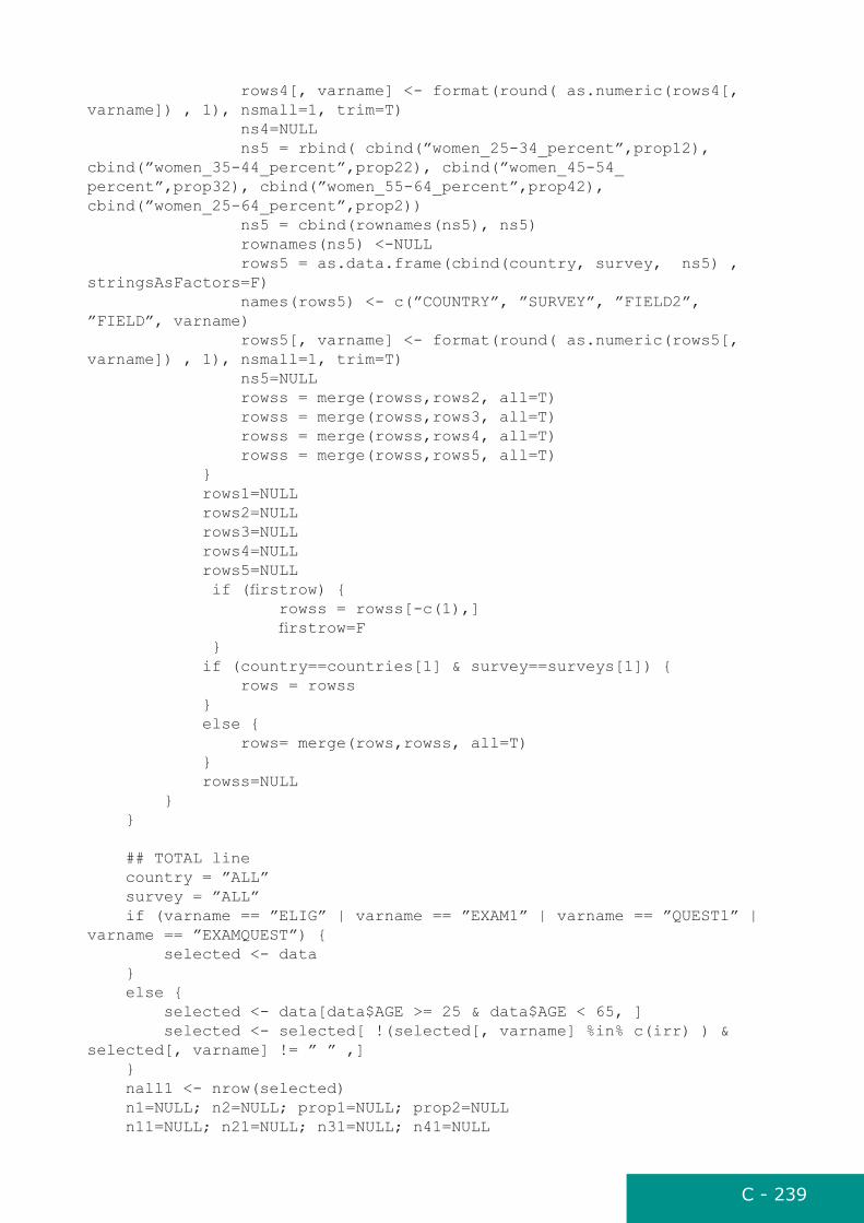
C - 239

rows4[, varname] <- format(round( as.numeric(rows4[, varname]) , 1), nsmall=1, trim=T) ns4=NULL ns5 = rbind( cbind(”women_25-34_percent”,prop12), cbind(”women_35-44_percent”,prop22), cbind(”women_45-54_percent”,prop32), cbind(”women_55-64_percent”,prop42), cbind(”women_25-64_percent”,prop2)) ns5 = cbind(rownames(ns5), ns5) rownames(ns5) <-NULL rows5 = as.data.frame(cbind(country, survey, ns5) , stringsAsFactors=F) names(rows5) <- c(”COUNTRY”, ”SURVEY”, ”FIELD2”, ”FIELD”, varname) rows5[, varname] <- format(round( as.numeric(rows5[, varname]) , 1), nsmall=1, trim=T) ns5=NULL rowss = merge(rowss,rows2, all=T) rowss = merge(rowss,rows3, all=T) rowss = merge(rowss,rows4, all=T) rowss = merge(rowss,rows5, all=T) } rows1=NULL rows2=NULL rows3=NULL rows4=NULL rows5=NULL if (firstrow) { rowss = rowss[-c(1),] firstrow=F } if (country==countries[1] & survey==surveys[1]) { rows = rowss } else { rows= merge(rows,rowss, all=T) } rowss=NULL } }

## TOTAL line country = ”ALL” survey = ”ALL” if (varname == ”ELIG” | varname == ”EXAM1” | varname == ”QUEST1” | varname == ”EXAMQUEST”) { selected <- data } else { selected <- data[data$AGE >= 25 & data$AGE < 65, ] selected <- selected[ !(selected[, varname] %in% c(irr) ) & selected[, varname] != ” ” ,] } nall1 <- nrow(selected) n1=NULL; n2=NULL; prop1=NULL; prop2=NULL n11=NULL; n21=NULL; n31=NULL; n41=NULL

C - 240

n12=NULL; n22=NULL; n32=NULL; n42=NULL prop11=NULL; prop21=NULL; prop31=NULL; prop41=NULL prop12=NULL; prop22=NULL; prop32=NULL; prop42=NULL nmen <- nrow(selected[ selected[, varname] %in% values & selected$SEX == ”1”,]) nwomen <- nrow(selected[ selected[, varname] %in% values & selected$SEX == ”2”,]) if (varname == ”ELIG” | varname == ”EXAM1” | varname == ”QUEST1” | varname == ”EXAMQUEST”) { nall <- nrow(selected[(selected$SEX %in% c(”1”,”2”)) & selected$AGE != ”999” & selected$AGE != ”” & selected[, varname] %in% values & selected$AGE >= 25 & selected$AGE < 65, ]) nmis <- nrow(selected[ !(selected$SEX %in% c(”1”,”2”)) | selected$AGE == ””| selected$AGE == ”999” | !(selected[, varname] %in% values) | selected$AGE < 25 | selected$AGE >= 65 , ]) nmen <- nrow(selected[ selected[, varname] %in% values & selected$SEX == ”1” & selected$AGE != ”999” & selected$AGE != ”” & selected$AGE >= 25 & selected$AGE < 65,]) nwomen <- nrow(selected[ selected[, varname] %in% values & selected$SEX == ”2” & selected$AGE != ”999” & selected$AGE != ”” & selected$AGE >= 25 & selected$AGE < 65,]) nmism = ”” nmisw =”” selected = selected[selected$SEX %in% c(”1”,”2”) & selected$AGE >= 25 & selected$AGE < 65,] } else { nall <- nrow(selected[ selected[, varname] %in% values,]) nmis <- nrow(selected[ selected[, varname] %in% mis,]) nmism <- nrow(selected[ selected[, varname] %in% mis & selected$SEX == ”1”,]) nmisw <- nrow(selected[ selected[, varname] %in% mis & selected$SEX == ”2”,]) } selected = selected[ !(selected[, varname] %in% c(mis)) , ] selected[, varname] <- as.numeric(selected[, varname]) age1 <- selected[selected$AGE >= 25 & selected$AGE < 35 , ] age2 <- selected[selected$AGE >= 35 & selected$AGE < 45 , ] age3 <- selected[selected$AGE >= 45 & selected$AGE < 55 , ] age4 <- selected[selected$AGE >= 55 & selected$AGE < 65 , ] if (nmen !=0 ) { n1[”all”] <- length(na.omit(selected[selected$SEX == ”1”, varname])) n11[”all”] <- length(na.omit(age1[age1$SEX == ”1”, varname])) n21[”all”] <- length(na.omit(age2[age2$SEX == ”1”, varname])) n31[”all”] <- length(na.omit(age3[age3$SEX == ”1”, varname])) n41[”all”] <- length(na.omit(age4[age4$SEX == ”1”, varname])) } if (nwomen !=0 ) { n2[”all”] <- length(na.omit(selected[selected$SEX == ”2”, varname])) n12[”all”] <- length(na.omit(age1[age1$SEX == ”2”, varname])) n22[”all”] <- length(na.omit(age2[age2$SEX == ”2”, varname])) n32[”all”] <- length(na.omit(age3[age3$SEX == ”2”, varname])) n42[”all”] <- length(na.omit(age4[age4$SEX == ”2”, varname]))

C - 241

} ns1 = c(nall, nmis, nmism, nmisw) rows1 = as.data.frame(cbind(country, survey, ns_header1, ”all”, ns1) , stringsAsFactors=F) names(rows1) <- c(”COUNTRY”, ”SURVEY”, ”FIELD”, ”FIELD2”, varname) ns1=NULL rows = merge(rows,rows1, all=T) rows1=NULL

if (nall != 0) { for (value in values) { if ( nall == 0) { n1[value] <- ””; n2[value] <- ”” n11[value] <- ””; n21[value] <- ””; n31[value] <- ””; n41[value] <- ””; n12[value] <- ””; n22[value] <- ””; n32[value] <- ””; n42[value] <- ”” prop1[value] <- ””; prop2[value] <- ””; prop11[value] <- ””; prop21[value] <- ””; prop31[value] <- ””; prop41[value] <- ”” prop12[value] <- ””; prop22[value] <- ””; prop32[value] <- ””; prop42[value] <- ”” } else { if (nmen !=0 ) { n1[value] <- length(na.omit(selected[selected$SEX == ”1” & selected[,varname] == value, varname])) n11[value] <- length(na.omit(age1[age1$SEX == ”1” & age1[,varname] == value, varname])) n21[value] <- length(na.omit(age2[age2$SEX == ”1” & age2[,varname] == value, varname])) n31[value] <- length(na.omit(age3[age3$SEX == ”1” & age3[,varname] == value, varname])) n41[value] <- length(na.omit(age4[age4$SEX == ”1” & age4[,varname] == value, varname])) prop11[value] <- 100*(n11[value] / n11[”all”]) prop21[value] <- 100*(n21[value] / n21[”all”] ) prop31[value] <- 100*(n31[value] / n31[”all”] ) prop41[value] <- 100*(n41[value] / n41[”all”] ) prop1[value] <- mean(c(prop11[value], prop21[value], prop31[value], prop41[value])) prop1[value] = format(round(as.numeric(prop1[value]), 1), nsmall=1) } else { prop1[value] = ”” prop11[value] = ”” prop21[value] = ”” prop31[value] = ”” prop41[value] = ”” n1[value] = ”0” n11[value] = ”0” n21[value] = ”0” n31[value] = ”0” n41[value] = ”0” } if (nwomen !=0 ) {

C - 242

n2[value] <- length(na.omit(selected[selected$SEX == ”2” & selected[,varname] == value, varname])) n12[value] <- length(na.omit(age1[age1$SEX == ”2” & age1[,varname] == value, varname])) n22[value] <- length(na.omit(age2[age2$SEX == ”2” & age2[,varname] == value, varname])) n32[value] <- length(na.omit(age3[age3$SEX == ”2” & age3[,varname] == value, varname])) n42[value] <- length(na.omit(age4[age4$SEX == ”2” & age4[,varname] == value, varname])) prop12[value] <- 100*(n12[value] / n12[”all”]) prop22[value] <- 100*(n22[value] / n22[”all”] ) prop32[value] <- 100*(n32[value] / n32[”all”] ) prop42[value] <- 100*(n42[value] / n42[”all”] ) prop2[value] <- mean(c(prop12[value], prop22[value], prop32[value], prop42[value])) prop2[value] = format(round(as.numeric(prop2[value]), 1), nsmall=1) } else { prop2[value] = ”” prop12[value] = ”” prop22[value] = ”” prop32[value] = ”” prop42[value] = ”” n2[value] = ”0” n12[value] = ”0” n22[value] = ”0” n32[value] = ”0” n42[value] = ”0” } } } ns2 = rbind( cbind(”men_25-34_n”,n11), cbind(”men_35-44_n”,n21), cbind(”men_45-54_n”,n31), cbind(”men_55-64_n”,n41), cbind(”men_25-64_n”,n1)) ns2 = cbind(rownames(ns2), ns2) rownames(ns2) <-NULL rows2 = as.data.frame(cbind(country, survey, ns2) , stringsAsFactors=F) names(rows2) <- c(”COUNTRY”, ”SURVEY”, ”FIELD2”, ”FIELD”, varname) ns2=NULL ns3 = rbind( cbind(”women_25-34_n”,n12), cbind(”women_35-44_n”,n22), cbind(”women_45-54_n”,n32), cbind(”women_55-64_n”,n42), cbind(”women_25-64_n”,n2)) ns3 = cbind(rownames(ns3), ns3) rownames(ns3) <-NULL rows3 = as.data.frame(cbind(country, survey, ns3) , stringsAsFactors=F) names(rows3) <- c(”COUNTRY”, ”SURVEY”, ”FIELD2”, ”FIELD”, varname) ns3=NULL ns4 = rbind( cbind(”men_25-34_percent”,prop11), cbind(”men_35-44_percent”,prop21), cbind(”men_45-54_percent”,prop31),

C - 243

cbind(”men_55-64_percent”,prop41), cbind(”men_25-64_percent”,prop1)) ns4 = cbind(rownames(ns4), ns4) rownames(ns4) <-NULL rows4 = as.data.frame(cbind(country, survey, ns4) , stringsAsFactors=F) names(rows4) <- c(”COUNTRY”, ”SURVEY”, ”FIELD2”, ”FIELD”, varname) rows4[, varname] <- format(round( as.numeric(rows4[, varname]) , 1), nsmall=1, trim=T) ns4=NULL ns5 = rbind( cbind(”women_25-34_percent”,prop12), cbind(”women_35-44_percent”,prop22), cbind(”women_45-54_percent”,prop32), cbind(”women_55-64_percent”,prop42), cbind(”women_25-64_percent”,prop2)) ns5 = cbind(rownames(ns5), ns5) rownames(ns5) <-NULL rows5 = as.data.frame(cbind(country, survey, ns5) , stringsAsFactors=F) names(rows5) <- c(”COUNTRY”, ”SURVEY”, ”FIELD2”, ”FIELD”, varname) rows5[, varname] <- format(round( as.numeric(rows5[, varname]) , 1), nsmall=1, trim=T) ns5=NULL rows = merge(rows,rows2, all=T) rows = merge(rows,rows3, all=T) rows = merge(rows,rows4, all=T) rows = merge(rows,rows5, all=T) } rows2=NULL rows3=NULL rows4=NULL rows5=NULL cat(’Prevalences for ’, varname, ’ done.\n’, sep=’’) return(rows)}

plotdist - to plot simple histogram of the variable

plotdist <- function(data, varname, outpath, div, minim, maxim, mis=NA, irr=NA, axmin=minim, axmax=maxim) { ### data = dataset, varname = name of the variable, outpath = path to save the file, minim = lower limit of the variable, maxim = upper limit of the variable, ### mis = code for missing value, irr = code for irrelevants, axmin = minimum of the x-axis, axmax = minimum of the x-axis return=T variable <-data[, varname] novalue <- (variable %in% mis) totallymis <- (variable %in% irr) if (sum(totallymis) + sum(novalue) == length(variable)) { return = FALSE } variable <- as.numeric(variable[!novalue & !totallymis]) if (sum(variable >= minim & variable <= maxim) == 0) { return = FALSE

C - 244

} counts <- table(variable[variable >= minim & variable <= maxim]) classes <- as.numeric(names(counts)) divpoints <- ((classes %% div) == 0) if (return) { png(file = paste(outpath, tolower(data$COUNTRY[1]), data$SURVEY[1], ’_’, tolower(varname), ’.png’, sep=’’), width=800, height=600) plot(classes, counts, type=’h’, axes=FALSE, main=paste(varname, ’ (’, data$COUNTRY[1], ’survey’, data$SURVEY[1], ’)’), xlab=varname, ylab=’N’, xlim=c(minim, maxim), ylim=c(0, max(counts))) points(classes, counts, cex=0.6) # Number of outliers in the right: outl <- sum(variable > maxim) if (outl > 0) mtext(paste(outl, ’ obs.\n>’, maxim, sep=’’), side=1, line=3, at=maxim, cex=0.9) # Number of outliers in the left: outl <- sum(variable < minim) if (outl > 0) mtext(paste(outl, ’ obs.\n<’, minim, sep=’’), side=1, line=3, at=minim, cex=0.9) ## Number of observations and missing values mtext(paste(’n_relevant = ’,length(variable) + sum(novalue, na.rm=T), sep=’’), side=3, line=-2, cex=0.9, adj=1) mtext(paste(sum(novalue), ’ missing’, sep=’’), side=3, line=-3, cex=0.9, adj=1) box() axis(1, at=seq(axmin, axmax, by=div), labels=seq(axmin, axmax, by=div), cex.axis=0.9) axis(2, cex.axis=0.9) mtext(paste(’Updated on’, Sys.Date()), side=3, line=0.3, adj=1, cex=0.9) dev.off() } variable = NULL}

drawtable_pr - to derive participation rates by survey, sex and 10-year age-group

drawtable_pr <- function(data) { ### data = dataset # tab, output table tab <- NULL countries <- sort(unique(data$COUNTRY)) exclude <- ”” for (country in countries) { surveys <- sort(unique(data[data$COUNTRY == country,]$SURVEY)) for (survey in surveys) { #### both sex selected <- data[data$COUNTRY == country & data$SURVEY ==

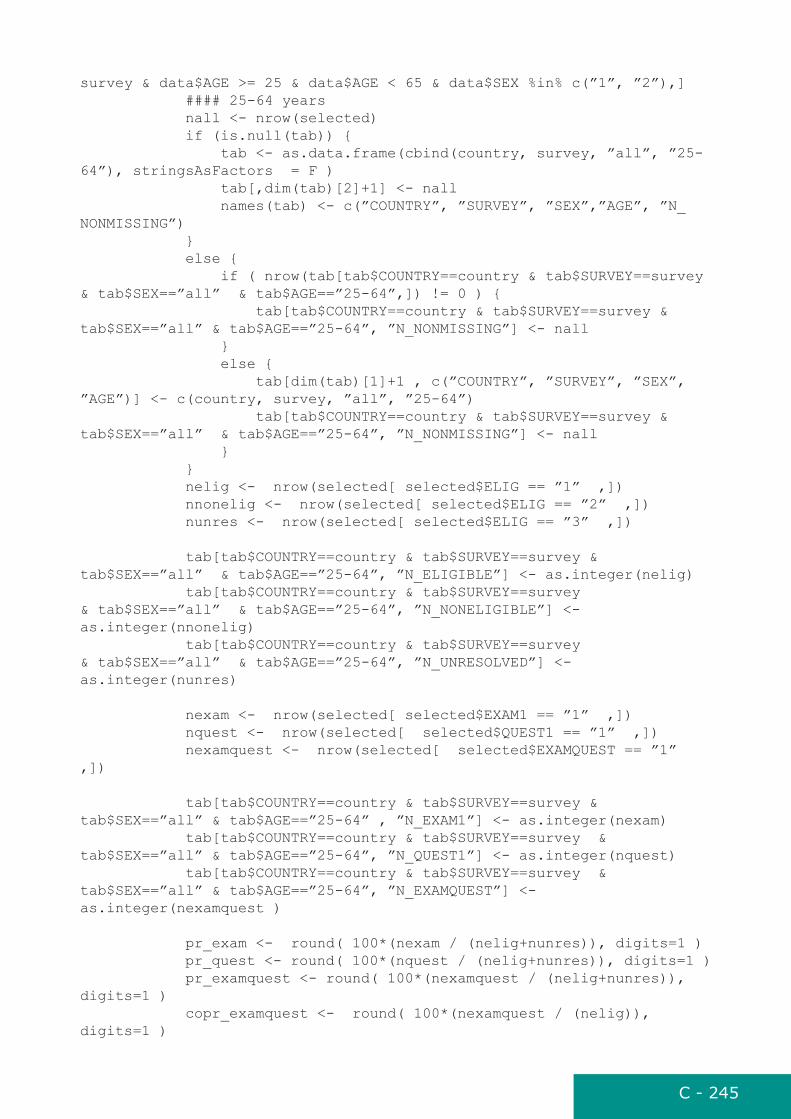
C - 245

survey & data$AGE >= 25 & data$AGE < 65 & data$SEX %in% c(”1”, ”2”),] #### 25-64 years nall <- nrow(selected) if (is.null(tab)) { tab <- as.data.frame(cbind(country, survey, ”all”, ”25-64”), stringsAsFactors = F ) tab[,dim(tab)[2]+1] <- nall names(tab) <- c(”COUNTRY”, ”SURVEY”, ”SEX”,”AGE”, ”N_NONMISSING”) } else { if ( nrow(tab[tab$COUNTRY==country & tab$SURVEY==survey & tab$SEX==”all” & tab$AGE==”25-64”,]) != 0 ) { tab[tab$COUNTRY==country & tab$SURVEY==survey & tab$SEX==”all” & tab$AGE==”25-64”, ”N_NONMISSING”] <- nall } else { tab[dim(tab)[1]+1 , c(”COUNTRY”, ”SURVEY”, ”SEX”, ”AGE”)] <- c(country, survey, ”all”, ”25-64”) tab[tab$COUNTRY==country & tab$SURVEY==survey & tab$SEX==”all” & tab$AGE==”25-64”, ”N_NONMISSING”] <- nall } } nelig <- nrow(selected[ selected$ELIG == ”1” ,]) nnonelig <- nrow(selected[ selected$ELIG == ”2” ,]) nunres <- nrow(selected[ selected$ELIG == ”3” ,])

tab[tab$COUNTRY==country & tab$SURVEY==survey & tab$SEX==”all” & tab$AGE==”25-64”, ”N_ELIGIBLE”] <- as.integer(nelig) tab[tab$COUNTRY==country & tab$SURVEY==survey & tab$SEX==”all” & tab$AGE==”25-64”, ”N_NONELIGIBLE”] <- as.integer(nnonelig) tab[tab$COUNTRY==country & tab$SURVEY==survey & tab$SEX==”all” & tab$AGE==”25-64”, ”N_UNRESOLVED”] <- as.integer(nunres)

nexam <- nrow(selected[ selected$EXAM1 == ”1” ,]) nquest <- nrow(selected[ selected$QUEST1 == ”1” ,]) nexamquest <- nrow(selected[ selected$EXAMQUEST == ”1” ,])

tab[tab$COUNTRY==country & tab$SURVEY==survey & tab$SEX==”all” & tab$AGE==”25-64” , ”N_EXAM1”] <- as.integer(nexam) tab[tab$COUNTRY==country & tab$SURVEY==survey & tab$SEX==”all” & tab$AGE==”25-64”, ”N_QUEST1”] <- as.integer(nquest) tab[tab$COUNTRY==country & tab$SURVEY==survey & tab$SEX==”all” & tab$AGE==”25-64”, ”N_EXAMQUEST”] <- as.integer(nexamquest )

pr_exam <- round( 100*(nexam / (nelig+nunres)), digits=1 ) pr_quest <- round( 100*(nquest / (nelig+nunres)), digits=1 ) pr_examquest <- round( 100*(nexamquest / (nelig+nunres)), digits=1 ) copr_examquest <- round( 100*(nexamquest / (nelig)), digits=1 )

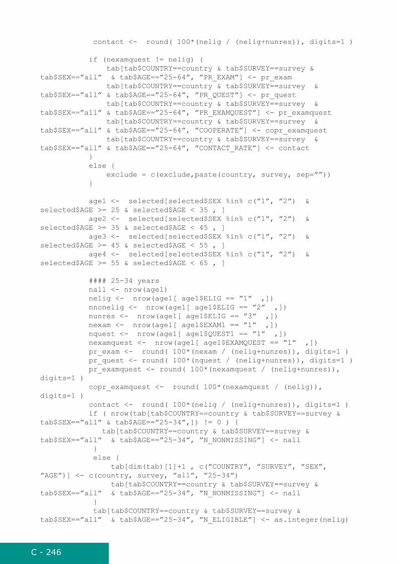
C - 246

contact <- round( 100*(nelig / (nelig+nunres)), digits=1 )

if (nexamquest != nelig) { tab[tab$COUNTRY==country & tab$SURVEY==survey & tab$SEX==”all” & tab$AGE==”25-64”, ”PR_EXAM”] <- pr_exam tab[tab$COUNTRY==country & tab$SURVEY==survey & tab$SEX==”all” & tab$AGE==”25-64”, ”PR_QUEST”] <- pr_quest tab[tab$COUNTRY==country & tab$SURVEY==survey & tab$SEX==”all” & tab$AGE==”25-64”, ”PR_EXAMQUEST”] <- pr_examquest tab[tab$COUNTRY==country & tab$SURVEY==survey & tab$SEX==”all” & tab$AGE==”25-64”, ”COOPERATE”] <- copr_examquest tab[tab$COUNTRY==country & tab$SURVEY==survey & tab$SEX==”all” & tab$AGE==”25-64”, ”CONTACT_RATE”] <- contact } else { exclude = c(exclude,paste(country, survey, sep=””)) }

age1 <- selected[selected$SEX %in% c(”1”, ”2”) & selected$AGE >= 25 & selected$AGE < 35 , ] age2 <- selected[selected$SEX %in% c(”1”, ”2”) & selected$AGE >= 35 & selected$AGE < 45 , ] age3 <- selected[selected$SEX %in% c(”1”, ”2”) & selected$AGE >= 45 & selected$AGE < 55 , ] age4 <- selected[selected$SEX %in% c(”1”, ”2”) & selected$AGE >= 55 & selected$AGE < 65 , ]

#### 25-34 years nall <- nrow(age1) nelig <- nrow(age1[ age1$ELIG == ”1” ,]) nnonelig <- nrow(age1[ age1$ELIG == ”2” ,]) nunres <- nrow(age1[ age1$ELIG == ”3” ,]) nexam <- nrow(age1[ age1$EXAM1 == ”1” ,]) nquest <- nrow(age1[ age1$QUEST1 == ”1” ,]) nexamquest <- nrow(age1[ age1$EXAMQUEST == ”1” ,]) pr_exam <- round( 100*(nexam / (nelig+nunres)), digits=1 ) pr_quest <- round( 100*(nquest / (nelig+nunres)), digits=1 ) pr_examquest <- round( 100*(nexamquest / (nelig+nunres)), digits=1 ) copr_examquest <- round( 100*(nexamquest / (nelig)), digits=1 ) contact <- round( 100*(nelig / (nelig+nunres)), digits=1 ) if ( nrow(tab[tab$COUNTRY==country & tab$SURVEY==survey & tab$SEX==”all” & tab$AGE==”25-34”,]) != 0 ) { tab[tab$COUNTRY==country & tab$SURVEY==survey & tab$SEX==”all” & tab$AGE==”25-34”, ”N_NONMISSING”] <- nall } else { tab[dim(tab)[1]+1 , c(”COUNTRY”, ”SURVEY”, ”SEX”, ”AGE”)] <- c(country, survey, ”all”, ”25-34”) tab[tab$COUNTRY==country & tab$SURVEY==survey & tab$SEX==”all” & tab$AGE==”25-34”, ”N_NONMISSING”] <- nall } tab[tab$COUNTRY==country & tab$SURVEY==survey & tab$SEX==”all” & tab$AGE==”25-34”, ”N_ELIGIBLE”] <- as.integer(nelig)

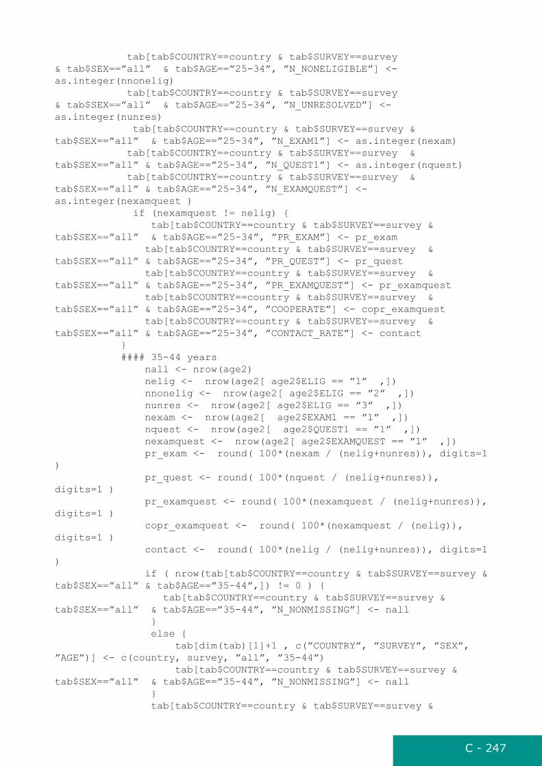
C - 247

tab[tab$COUNTRY==country & tab$SURVEY==survey & tab$SEX==”all” & tab$AGE==”25-34”, ”N_NONELIGIBLE”] <- as.integer(nnonelig) tab[tab$COUNTRY==country & tab$SURVEY==survey & tab$SEX==”all” & tab$AGE==”25-34”, ”N_UNRESOLVED”] <- as.integer(nunres) tab[tab$COUNTRY==country & tab$SURVEY==survey & tab$SEX==”all” & tab$AGE==”25-34”, ”N_EXAM1”] <- as.integer(nexam) tab[tab$COUNTRY==country & tab$SURVEY==survey & tab$SEX==”all” & tab$AGE==”25-34”, ”N_QUEST1”] <- as.integer(nquest) tab[tab$COUNTRY==country & tab$SURVEY==survey & tab$SEX==”all” & tab$AGE==”25-34”, ”N_EXAMQUEST”] <- as.integer(nexamquest ) if (nexamquest != nelig) { tab[tab$COUNTRY==country & tab$SURVEY==survey & tab$SEX==”all” & tab$AGE==”25-34”, ”PR_EXAM”] <- pr_exam tab[tab$COUNTRY==country & tab$SURVEY==survey & tab$SEX==”all” & tab$AGE==”25-34”, ”PR_QUEST”] <- pr_quest tab[tab$COUNTRY==country & tab$SURVEY==survey & tab$SEX==”all” & tab$AGE==”25-34”, ”PR_EXAMQUEST”] <- pr_examquest tab[tab$COUNTRY==country & tab$SURVEY==survey & tab$SEX==”all” & tab$AGE==”25-34”, ”COOPERATE”] <- copr_examquest tab[tab$COUNTRY==country & tab$SURVEY==survey & tab$SEX==”all” & tab$AGE==”25-34”, ”CONTACT_RATE”] <- contact } #### 35-44 years nall <- nrow(age2) nelig <- nrow(age2[ age2$ELIG == ”1” ,]) nnonelig <- nrow(age2[ age2$ELIG == ”2” ,]) nunres <- nrow(age2[ age2$ELIG == ”3” ,]) nexam <- nrow(age2[ age2$EXAM1 == ”1” ,]) nquest <- nrow(age2[ age2$QUEST1 == ”1” ,]) nexamquest <- nrow(age2[ age2$EXAMQUEST == ”1” ,]) pr_exam <- round( 100*(nexam / (nelig+nunres)), digits=1 ) pr_quest <- round( 100*(nquest / (nelig+nunres)), digits=1 ) pr_examquest <- round( 100*(nexamquest / (nelig+nunres)), digits=1 ) copr_examquest <- round( 100*(nexamquest / (nelig)), digits=1 ) contact <- round( 100*(nelig / (nelig+nunres)), digits=1 ) if ( nrow(tab[tab$COUNTRY==country & tab$SURVEY==survey & tab$SEX==”all” & tab$AGE==”35-44”,]) != 0 ) { tab[tab$COUNTRY==country & tab$SURVEY==survey & tab$SEX==”all” & tab$AGE==”35-44”, ”N_NONMISSING”] <- nall } else { tab[dim(tab)[1]+1 , c(”COUNTRY”, ”SURVEY”, ”SEX”, ”AGE”)] <- c(country, survey, ”all”, ”35-44”) tab[tab$COUNTRY==country & tab$SURVEY==survey & tab$SEX==”all” & tab$AGE==”35-44”, ”N_NONMISSING”] <- nall } tab[tab$COUNTRY==country & tab$SURVEY==survey &

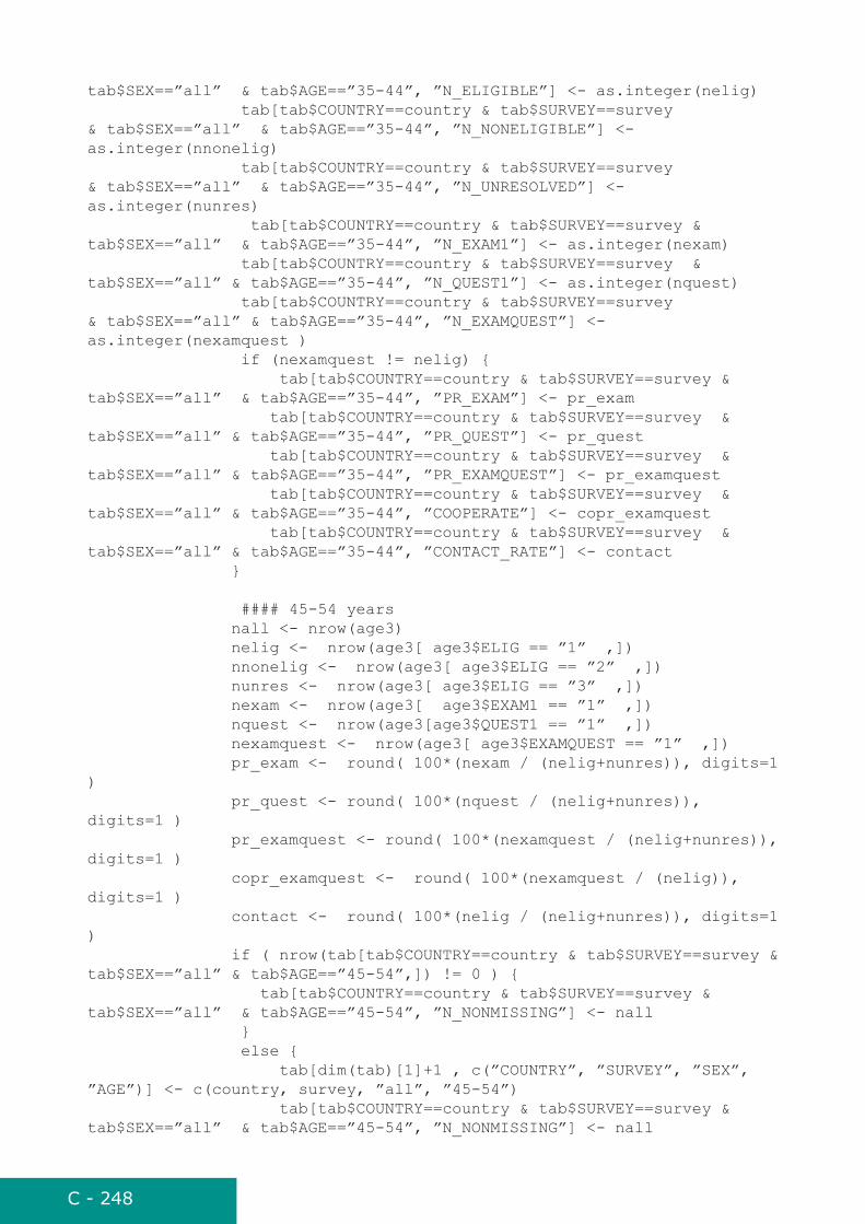
C - 248

tab$SEX==”all” & tab$AGE==”35-44”, ”N_ELIGIBLE”] <- as.integer(nelig) tab[tab$COUNTRY==country & tab$SURVEY==survey & tab$SEX==”all” & tab$AGE==”35-44”, ”N_NONELIGIBLE”] <- as.integer(nnonelig) tab[tab$COUNTRY==country & tab$SURVEY==survey & tab$SEX==”all” & tab$AGE==”35-44”, ”N_UNRESOLVED”] <- as.integer(nunres) tab[tab$COUNTRY==country & tab$SURVEY==survey & tab$SEX==”all” & tab$AGE==”35-44”, ”N_EXAM1”] <- as.integer(nexam) tab[tab$COUNTRY==country & tab$SURVEY==survey & tab$SEX==”all” & tab$AGE==”35-44”, ”N_QUEST1”] <- as.integer(nquest) tab[tab$COUNTRY==country & tab$SURVEY==survey & tab$SEX==”all” & tab$AGE==”35-44”, ”N_EXAMQUEST”] <- as.integer(nexamquest ) if (nexamquest != nelig) { tab[tab$COUNTRY==country & tab$SURVEY==survey & tab$SEX==”all” & tab$AGE==”35-44”, ”PR_EXAM”] <- pr_exam tab[tab$COUNTRY==country & tab$SURVEY==survey & tab$SEX==”all” & tab$AGE==”35-44”, ”PR_QUEST”] <- pr_quest tab[tab$COUNTRY==country & tab$SURVEY==survey & tab$SEX==”all” & tab$AGE==”35-44”, ”PR_EXAMQUEST”] <- pr_examquest tab[tab$COUNTRY==country & tab$SURVEY==survey & tab$SEX==”all” & tab$AGE==”35-44”, ”COOPERATE”] <- copr_examquest tab[tab$COUNTRY==country & tab$SURVEY==survey & tab$SEX==”all” & tab$AGE==”35-44”, ”CONTACT_RATE”] <- contact }

#### 45-54 years nall <- nrow(age3) nelig <- nrow(age3[ age3$ELIG == ”1” ,]) nnonelig <- nrow(age3[ age3$ELIG == ”2” ,]) nunres <- nrow(age3[ age3$ELIG == ”3” ,]) nexam <- nrow(age3[ age3$EXAM1 == ”1” ,]) nquest <- nrow(age3[age3$QUEST1 == ”1” ,]) nexamquest <- nrow(age3[ age3$EXAMQUEST == ”1” ,]) pr_exam <- round( 100*(nexam / (nelig+nunres)), digits=1 ) pr_quest <- round( 100*(nquest / (nelig+nunres)), digits=1 ) pr_examquest <- round( 100*(nexamquest / (nelig+nunres)), digits=1 ) copr_examquest <- round( 100*(nexamquest / (nelig)), digits=1 ) contact <- round( 100*(nelig / (nelig+nunres)), digits=1 ) if ( nrow(tab[tab$COUNTRY==country & tab$SURVEY==survey & tab$SEX==”all” & tab$AGE==”45-54”,]) != 0 ) { tab[tab$COUNTRY==country & tab$SURVEY==survey & tab$SEX==”all” & tab$AGE==”45-54”, ”N_NONMISSING”] <- nall } else { tab[dim(tab)[1]+1 , c(”COUNTRY”, ”SURVEY”, ”SEX”, ”AGE”)] <- c(country, survey, ”all”, ”45-54”) tab[tab$COUNTRY==country & tab$SURVEY==survey & tab$SEX==”all” & tab$AGE==”45-54”, ”N_NONMISSING”] <- nall

C - 249

} tab[tab$COUNTRY==country & tab$SURVEY==survey & tab$SEX==”all” & tab$AGE==”45-54”, ”N_ELIGIBLE”] <- as.integer(nelig) tab[tab$COUNTRY==country & tab$SURVEY==survey & tab$SEX==”all” & tab$AGE==”45-54”, ”N_NONELIGIBLE”] <- as.integer(nnonelig) tab[tab$COUNTRY==country & tab$SURVEY==survey & tab$SEX==”all” & tab$AGE==”45-54”, ”N_UNRESOLVED”] <- as.integer(nunres) tab[tab$COUNTRY==country & tab$SURVEY==survey & tab$SEX==”all” & tab$AGE==”45-54”, ”N_EXAM1”] <- as.integer(nexam) tab[tab$COUNTRY==country & tab$SURVEY==survey & tab$SEX==”all” & tab$AGE==”45-54”, ”N_QUEST1”] <- as.integer(nquest) tab[tab$COUNTRY==country & tab$SURVEY==survey & tab$SEX==”all” & tab$AGE==”45-54”, ”N_EXAMQUEST”] <- as.integer(nexamquest ) if (nexamquest != nelig) { tab[tab$COUNTRY==country & tab$SURVEY==survey & tab$SEX==”all” & tab$AGE==”45-54”, ”PR_EXAM”] <- pr_exam tab[tab$COUNTRY==country & tab$SURVEY==survey & tab$SEX==”all” & tab$AGE==”45-54”, ”PR_QUEST”] <- pr_quest tab[tab$COUNTRY==country & tab$SURVEY==survey & tab$SEX==”all” & tab$AGE==”45-54”, ”PR_EXAMQUEST”] <- pr_examquest tab[tab$COUNTRY==country & tab$SURVEY==survey & tab$SEX==”all” & tab$AGE==”45-54”, ”COOPERATE”] <- copr_examquest tab[tab$COUNTRY==country & tab$SURVEY==survey & tab$SEX==”all” & tab$AGE==”45-54”, ”CONTACT_RATE”] <- contact }

#### 55-64 years nall <- nrow(age4) nelig <- nrow(age4[ age4$ELIG == ”1” ,]) nnonelig <- nrow(age4[ age4$ELIG == ”2” ,]) nunres <- nrow(age4[ age4$ELIG == ”3” ,]) nexam <- nrow(age4[ age4$EXAM1 == ”1” ,]) nquest <- nrow(age4[ age4$QUEST1 == ”1” ,]) nexamquest <- nrow(age4[ age4$EXAMQUEST == ”1” ,]) pr_exam <- round( 100*(nexam / (nelig+nunres)), digits=1 ) pr_quest <- round( 100*(nquest / (nelig+nunres)), digits=1 ) pr_examquest <- round( 100*(nexamquest / (nelig+nunres)), digits=1 ) copr_examquest <- round( 100*(nexamquest / (nelig)), digits=1 ) contact <- round( 100*(nelig / (nelig+nunres)), digits=1 ) if ( nrow(tab[tab$COUNTRY==country & tab$SURVEY==survey & tab$SEX==”all” & tab$AGE==”55-64”,]) != 0 ) { tab[tab$COUNTRY==country & tab$SURVEY==survey & tab$SEX==”all” & tab$AGE==”55-64”, ”N_NONMISSING”] <- nall } else { tab[dim(tab)[1]+1 , c(”COUNTRY”, ”SURVEY”, ”SEX”, ”AGE”)] <- c(country, survey, ”all”, ”55-64”)

C - 250

tab[tab$COUNTRY==country & tab$SURVEY==survey & tab$SEX==”all” & tab$AGE==”55-64”, ”N_NONMISSING”] <- nall } tab[tab$COUNTRY==country & tab$SURVEY==survey & tab$SEX==”all” & tab$AGE==”55-64”, ”N_ELIGIBLE”] <- as.integer(nelig) tab[tab$COUNTRY==country & tab$SURVEY==survey & tab$SEX==”all” & tab$AGE==”55-64”, ”N_NONELIGIBLE”] <- as.integer(nnonelig) tab[tab$COUNTRY==country & tab$SURVEY==survey & tab$SEX==”all” & tab$AGE==”55-64”, ”N_UNRESOLVED”] <- as.integer(nunres) tab[tab$COUNTRY==country & tab$SURVEY==survey & tab$SEX==”all” & tab$AGE==”55-64”, ”N_EXAM1”] <- as.integer(nexam) tab[tab$COUNTRY==country & tab$SURVEY==survey & tab$SEX==”all” & tab$AGE==”55-64”, ”N_QUEST1”] <- as.integer(nquest) tab[tab$COUNTRY==country & tab$SURVEY==survey & tab$SEX==”all” & tab$AGE==”55-64”, ”N_EXAMQUEST”] <- as.integer(nexamquest ) if (nexamquest != nelig) { tab[tab$COUNTRY==country & tab$SURVEY==survey & tab$SEX==”all” & tab$AGE==”55-64”, ”PR_EXAM”] <- pr_exam tab[tab$COUNTRY==country & tab$SURVEY==survey & tab$SEX==”all” & tab$AGE==”55-64”, ”PR_QUEST”] <- pr_quest tab[tab$COUNTRY==country & tab$SURVEY==survey & tab$SEX==”all” & tab$AGE==”55-64”, ”PR_EXAMQUEST”] <- pr_examquest tab[tab$COUNTRY==country & tab$SURVEY==survey & tab$SEX==”all” & tab$AGE==”55-64”, ”COOPERATE”] <- copr_examquest tab[tab$COUNTRY==country & tab$SURVEY==survey & tab$SEX==”all” & tab$AGE==”55-64”, ”CONTACT_RATE”] <- contact } age1=NULL age2=NULL age3=NULL age4=NULL

for (sex in c(”1”, ”2”)) { selected1 <- selected[selected$SEX == sex ,] if (sex == ”1”) { sex2 <- ”men” } else {sex2 <- ”women”} nall <- nrow(selected1) if ( nrow(tab[tab$COUNTRY==country & tab$SURVEY==survey & tab$SEX==sex2 & tab$AGE==”25-64”,]) != 0 ) { tab[tab$COUNTRY==country & tab$SURVEY==survey & tab$SEX==sex2 & tab$AGE==”25-64”, ”N_NONMISSING”] <- nall } else { tab[dim(tab)[1]+1 , c(”COUNTRY”, ”SURVEY”, ”SEX”, ”AGE”)] <- c(country, survey, sex2, ”25-64”) tab[tab$COUNTRY==country & tab$SURVEY==survey & tab$SEX==sex2 & tab$AGE==”25-64”, ”N_NONMISSING”] <- nall } nelig <- nrow(selected1[ selected1$ELIG == ”1” ,]) nnonelig <- nrow(selected1[ selected1$ELIG == ”2” ,])

C - 251

nunres <- nrow(selected1[ selected1$ELIG == ”3” ,])

tab[tab$COUNTRY==country & tab$SURVEY==survey & tab$SEX==sex2 & tab$AGE==”25-64”, ”N_ELIGIBLE”] <- as.integer(nelig) tab[tab$COUNTRY==country & tab$SURVEY==survey & tab$SEX==sex2 & tab$AGE==”25-64”, ”N_NONELIGIBLE”] <- as.integer(nnonelig) tab[tab$COUNTRY==country & tab$SURVEY==survey & tab$SEX==sex2 & tab$AGE==”25-64”, ”N_UNRESOLVED”] <- as.integer(nunres)

nexam <- nrow(selected1[ selected1$EXAM1 == ”1” ,]) nquest <- nrow(selected1[ selected1$QUEST1 == ”1” ,]) nexamquest <- nrow(selected1[selected1$EXAMQUEST == ”1” ,])

tab[tab$COUNTRY==country & tab$SURVEY==survey & tab$SEX==sex2 & tab$AGE==”25-64”, ”N_EXAM1”] <- as.integer(nexam) tab[tab$COUNTRY==country & tab$SURVEY==survey & tab$SEX==sex2 & tab$AGE==”25-64”, ”N_QUEST1”] <- as.integer(nquest) tab[tab$COUNTRY==country & tab$SURVEY==survey & tab$SEX==sex2 & tab$AGE==”25-64”, ”N_EXAMQUEST”] <- as.integer(nexamquest )

pr_exam <- round( 100*(nexam / (nelig+nunres)), digits=1 ) pr_quest <- round( 100*(nquest / (nelig+nunres)), digits=1 ) pr_examquest <- round( 100*(nexamquest / (nelig+nunres)), digits=1 ) copr_examquest <- round( 100*(nexamquest / (nelig)), digits=1 ) contact <- round( 100*(nelig / (nelig+nunres)), digits=1 )

if (nexamquest != nelig) { tab[tab$COUNTRY==country & tab$SURVEY==survey & tab$SEX==sex2 & tab$AGE==”25-64”, ”PR_EXAM”] <- pr_exam tab[tab$COUNTRY==country & tab$SURVEY==survey & tab$SEX==sex2 & tab$AGE==”25-64”, ”PR_QUEST”] <- pr_quest tab[tab$COUNTRY==country & tab$SURVEY==survey & tab$SEX==sex2 & tab$AGE==”25-64”, ”PR_EXAMQUEST”] <- pr_examquest tab[tab$COUNTRY==country & tab$SURVEY==survey & tab$SEX==sex2 & tab$AGE==”25-64”, ”COOPERATE”] <- copr_examquest tab[tab$COUNTRY==country & tab$SURVEY==survey & tab$SEX==sex2 & tab$AGE==”25-64”, ”CONTACT_RATE”] <- contact }

age1 <- selected1[selected1$AGE >= 25 & selected1$AGE < 35 , ] age2 <- selected1[selected1$AGE >= 35 & selected1$AGE < 45 , ] age3 <- selected1[selected1$AGE >= 45 & selected1$AGE < 55 , ] age4 <- selected1[selected1$AGE >= 55 & selected1$AGE < 65 , ]

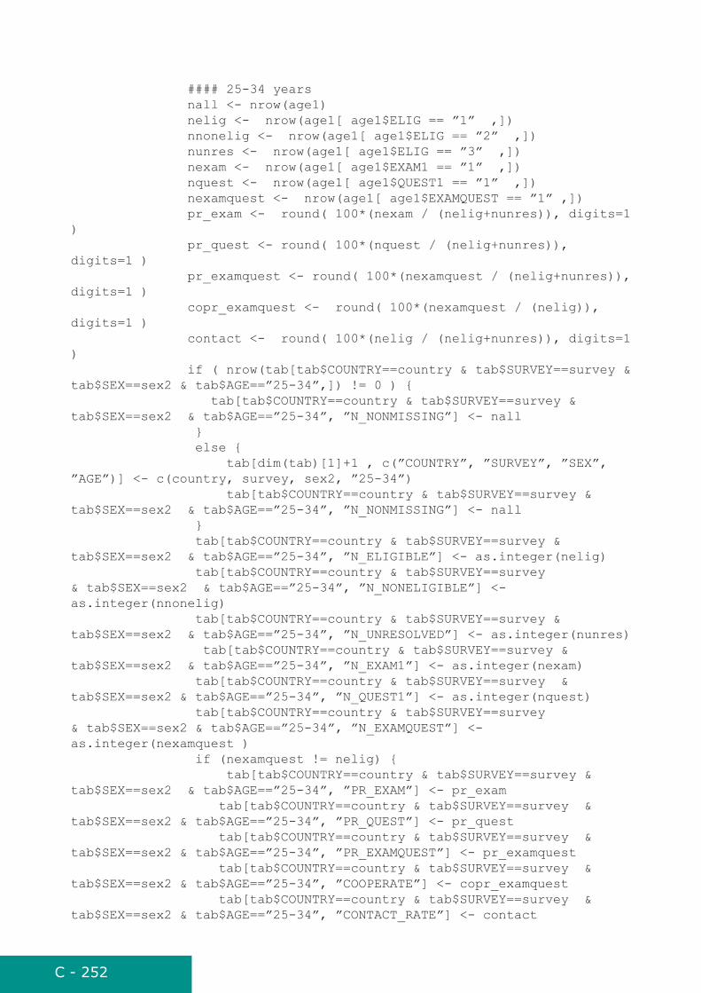
C - 252

#### 25-34 years nall <- nrow(age1) nelig <- nrow(age1[ age1$ELIG == ”1” ,]) nnonelig <- nrow(age1[ age1$ELIG == ”2” ,]) nunres <- nrow(age1[ age1$ELIG == ”3” ,]) nexam <- nrow(age1[ age1$EXAM1 == ”1” ,]) nquest <- nrow(age1[ age1$QUEST1 == ”1” ,]) nexamquest <- nrow(age1[ age1$EXAMQUEST == ”1” ,]) pr_exam <- round( 100*(nexam / (nelig+nunres)), digits=1 ) pr_quest <- round( 100*(nquest / (nelig+nunres)), digits=1 ) pr_examquest <- round( 100*(nexamquest / (nelig+nunres)), digits=1 ) copr_examquest <- round( 100*(nexamquest / (nelig)), digits=1 ) contact <- round( 100*(nelig / (nelig+nunres)), digits=1 ) if ( nrow(tab[tab$COUNTRY==country & tab$SURVEY==survey & tab$SEX==sex2 & tab$AGE==”25-34”,]) != 0 ) { tab[tab$COUNTRY==country & tab$SURVEY==survey & tab$SEX==sex2 & tab$AGE==”25-34”, ”N_NONMISSING”] <- nall } else { tab[dim(tab)[1]+1 , c(”COUNTRY”, ”SURVEY”, ”SEX”, ”AGE”)] <- c(country, survey, sex2, ”25-34”) tab[tab$COUNTRY==country & tab$SURVEY==survey & tab$SEX==sex2 & tab$AGE==”25-34”, ”N_NONMISSING”] <- nall } tab[tab$COUNTRY==country & tab$SURVEY==survey & tab$SEX==sex2 & tab$AGE==”25-34”, ”N_ELIGIBLE”] <- as.integer(nelig) tab[tab$COUNTRY==country & tab$SURVEY==survey & tab$SEX==sex2 & tab$AGE==”25-34”, ”N_NONELIGIBLE”] <- as.integer(nnonelig) tab[tab$COUNTRY==country & tab$SURVEY==survey & tab$SEX==sex2 & tab$AGE==”25-34”, ”N_UNRESOLVED”] <- as.integer(nunres) tab[tab$COUNTRY==country & tab$SURVEY==survey & tab$SEX==sex2 & tab$AGE==”25-34”, ”N_EXAM1”] <- as.integer(nexam) tab[tab$COUNTRY==country & tab$SURVEY==survey & tab$SEX==sex2 & tab$AGE==”25-34”, ”N_QUEST1”] <- as.integer(nquest) tab[tab$COUNTRY==country & tab$SURVEY==survey & tab$SEX==sex2 & tab$AGE==”25-34”, ”N_EXAMQUEST”] <- as.integer(nexamquest ) if (nexamquest != nelig) { tab[tab$COUNTRY==country & tab$SURVEY==survey & tab$SEX==sex2 & tab$AGE==”25-34”, ”PR_EXAM”] <- pr_exam tab[tab$COUNTRY==country & tab$SURVEY==survey & tab$SEX==sex2 & tab$AGE==”25-34”, ”PR_QUEST”] <- pr_quest tab[tab$COUNTRY==country & tab$SURVEY==survey & tab$SEX==sex2 & tab$AGE==”25-34”, ”PR_EXAMQUEST”] <- pr_examquest tab[tab$COUNTRY==country & tab$SURVEY==survey & tab$SEX==sex2 & tab$AGE==”25-34”, ”COOPERATE”] <- copr_examquest tab[tab$COUNTRY==country & tab$SURVEY==survey & tab$SEX==sex2 & tab$AGE==”25-34”, ”CONTACT_RATE”] <- contact

C - 253

}

#### 35-44 years nall <- nrow(age2) nelig <- nrow(age2[ age2$ELIG == ”1” ,]) nnonelig <- nrow(age2[ age2$ELIG == ”2” ,]) nunres <- nrow(age2[ age2$ELIG == ”3” ,]) nexam <- nrow(age2[ age2$EXAM1 == ”1” ,]) nquest <- nrow(age2[ age2$QUEST1 == ”1” ,]) nexamquest <- nrow(age2[ age2$EXAMQUEST == ”1” ,]) pr_exam <- round( 100*(nexam / (nelig+nunres)), digits=1 ) pr_quest <- round( 100*(nquest / (nelig+nunres)), digits=1 ) pr_examquest <- round( 100*(nexamquest / (nelig+nunres)), digits=1 ) copr_examquest <- round( 100*(nexamquest / (nelig)), digits=1 ) contact <- round( 100*(nelig / (nelig+nunres)), digits=1 ) if ( nrow(tab[tab$COUNTRY==country & tab$SURVEY==survey & tab$SEX==sex2 & tab$AGE==”35-44”,]) != 0 ) { tab[tab$COUNTRY==country & tab$SURVEY==survey & tab$SEX==sex2 & tab$AGE==”35-44”, ”N_NONMISSING”] <- nall } else { tab[dim(tab)[1]+1 , c(”COUNTRY”, ”SURVEY”, ”SEX”, ”AGE”)] <- c(country, survey, sex2, ”35-44”) tab[tab$COUNTRY==country & tab$SURVEY==survey & tab$SEX==sex2 & tab$AGE==”35-44”, ”N_NONMISSING”] <- nall } tab[tab$COUNTRY==country & tab$SURVEY==survey & tab$SEX==sex2 & tab$AGE==”35-44”, ”N_ELIGIBLE”] <- as.integer(nelig) tab[tab$COUNTRY==country & tab$SURVEY==survey & tab$SEX==sex2 & tab$AGE==”35-44”, ”N_NONELIGIBLE”] <- as.integer(nnonelig) tab[tab$COUNTRY==country & tab$SURVEY==survey & tab$SEX==sex2 & tab$AGE==”35-44”, ”N_UNRESOLVED”] <- as.integer(nunres) tab[tab$COUNTRY==country & tab$SURVEY==survey & tab$SEX==sex2 & tab$AGE==”35-44”, ”N_EXAM1”] <- as.integer(nexam) tab[tab$COUNTRY==country & tab$SURVEY==survey & tab$SEX==sex2 & tab$AGE==”35-44”, ”N_QUEST1”] <- as.integer(nquest) tab[tab$COUNTRY==country & tab$SURVEY==survey & tab$SEX==sex2 & tab$AGE==”35-44”, ”N_EXAMQUEST”] <- as.integer(nexamquest ) if (nexamquest != nelig) { tab[tab$COUNTRY==country & tab$SURVEY==survey & tab$SEX==sex2 & tab$AGE==”35-44”, ”PR_EXAM”] <- pr_exam tab[tab$COUNTRY==country & tab$SURVEY==survey & tab$SEX==sex2 & tab$AGE==”35-44”, ”PR_QUEST”] <- pr_quest tab[tab$COUNTRY==country & tab$SURVEY==survey & tab$SEX==sex2 & tab$AGE==”35-44”, ”PR_EXAMQUEST”] <- pr_examquest tab[tab$COUNTRY==country & tab$SURVEY==survey & tab$SEX==sex2 & tab$AGE==”35-44”, ”COOPERATE”] <- copr_examquest tab[tab$COUNTRY==country & tab$SURVEY==survey &

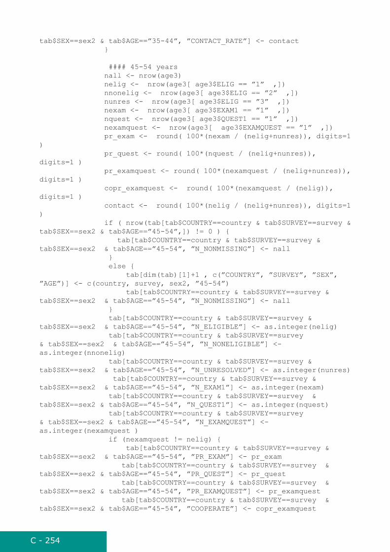
C - 254

tab$SEX==sex2 & tab$AGE==”35-44”, ”CONTACT_RATE”] <- contact }

#### 45-54 years nall <- nrow(age3) nelig <- nrow(age3[ age3$ELIG == ”1” ,]) nnonelig <- nrow(age3[ age3$ELIG == ”2” ,]) nunres <- nrow(age3[ age3$ELIG == ”3” ,]) nexam <- nrow(age3[ age3$EXAM1 == ”1” ,]) nquest <- nrow(age3[ age3$QUEST1 == ”1” ,]) nexamquest <- nrow(age3[ age3$EXAMQUEST == ”1” ,]) pr_exam <- round( 100*(nexam / (nelig+nunres)), digits=1 ) pr_quest <- round( 100*(nquest / (nelig+nunres)), digits=1 ) pr_examquest <- round( 100*(nexamquest / (nelig+nunres)), digits=1 ) copr_examquest <- round( 100*(nexamquest / (nelig)), digits=1 ) contact <- round( 100*(nelig / (nelig+nunres)), digits=1 ) if ( nrow(tab[tab$COUNTRY==country & tab$SURVEY==survey & tab$SEX==sex2 & tab$AGE==”45-54”,]) != 0 ) { tab[tab$COUNTRY==country & tab$SURVEY==survey & tab$SEX==sex2 & tab$AGE==”45-54”, ”N_NONMISSING”] <- nall } else { tab[dim(tab)[1]+1 , c(”COUNTRY”, ”SURVEY”, ”SEX”, ”AGE”)] <- c(country, survey, sex2, ”45-54”) tab[tab$COUNTRY==country & tab$SURVEY==survey & tab$SEX==sex2 & tab$AGE==”45-54”, ”N_NONMISSING”] <- nall } tab[tab$COUNTRY==country & tab$SURVEY==survey & tab$SEX==sex2 & tab$AGE==”45-54”, ”N_ELIGIBLE”] <- as.integer(nelig) tab[tab$COUNTRY==country & tab$SURVEY==survey & tab$SEX==sex2 & tab$AGE==”45-54”, ”N_NONELIGIBLE”] <- as.integer(nnonelig) tab[tab$COUNTRY==country & tab$SURVEY==survey & tab$SEX==sex2 & tab$AGE==”45-54”, ”N_UNRESOLVED”] <- as.integer(nunres) tab[tab$COUNTRY==country & tab$SURVEY==survey & tab$SEX==sex2 & tab$AGE==”45-54”, ”N_EXAM1”] <- as.integer(nexam) tab[tab$COUNTRY==country & tab$SURVEY==survey & tab$SEX==sex2 & tab$AGE==”45-54”, ”N_QUEST1”] <- as.integer(nquest) tab[tab$COUNTRY==country & tab$SURVEY==survey & tab$SEX==sex2 & tab$AGE==”45-54”, ”N_EXAMQUEST”] <- as.integer(nexamquest ) if (nexamquest != nelig) { tab[tab$COUNTRY==country & tab$SURVEY==survey & tab$SEX==sex2 & tab$AGE==”45-54”, ”PR_EXAM”] <- pr_exam tab[tab$COUNTRY==country & tab$SURVEY==survey & tab$SEX==sex2 & tab$AGE==”45-54”, ”PR_QUEST”] <- pr_quest tab[tab$COUNTRY==country & tab$SURVEY==survey & tab$SEX==sex2 & tab$AGE==”45-54”, ”PR_EXAMQUEST”] <- pr_examquest tab[tab$COUNTRY==country & tab$SURVEY==survey & tab$SEX==sex2 & tab$AGE==”45-54”, ”COOPERATE”] <- copr_examquest

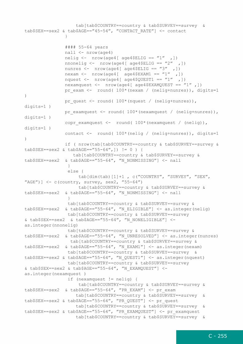
C - 255

tab[tab$COUNTRY==country & tab$SURVEY==survey & tab$SEX==sex2 & tab$AGE==”45-54”, ”CONTACT_RATE”] <- contact }

#### 55-64 years nall <- nrow(age4) nelig <- nrow(age4[ age4$ELIG == ”1” ,]) nnonelig <- nrow(age4[ age4$ELIG == ”2” ,]) nunres <- nrow(age4[ age4$ELIG == ”3” ,]) nexam <- nrow(age4[ age4$EXAM1 == ”1” ,]) nquest <- nrow(age4[ age4$QUEST1 == ”1” ,]) nexamquest <- nrow(age4[ age4$EXAMQUEST == ”1” ,]) pr_exam <- round( 100*(nexam / (nelig+nunres)), digits=1 ) pr_quest <- round( 100*(nquest / (nelig+nunres)), digits=1 ) pr_examquest <- round( 100*(nexamquest / (nelig+nunres)), digits=1 ) copr_examquest <- round( 100*(nexamquest / (nelig)), digits=1 ) contact <- round( 100*(nelig / (nelig+nunres)), digits=1 ) if ( nrow(tab[tab$COUNTRY==country & tab$SURVEY==survey & tab$SEX==sex2 & tab$AGE==”55-64”,]) != 0 ) { tab[tab$COUNTRY==country & tab$SURVEY==survey & tab$SEX==sex2 & tab$AGE==”55-64”, ”N_NONMISSING”] <- nall } else { tab[dim(tab)[1]+1 , c(”COUNTRY”, ”SURVEY”, ”SEX”, ”AGE”)] <- c(country, survey, sex2, ”55-64”) tab[tab$COUNTRY==country & tab$SURVEY==survey & tab$SEX==sex2 & tab$AGE==”55-64”, ”N_NONMISSING”] <- nall } tab[tab$COUNTRY==country & tab$SURVEY==survey & tab$SEX==sex2 & tab$AGE==”55-64”, ”N_ELIGIBLE”] <- as.integer(nelig) tab[tab$COUNTRY==country & tab$SURVEY==survey & tab$SEX==sex2 & tab$AGE==”55-64”, ”N_NONELIGIBLE”] <- as.integer(nnonelig) tab[tab$COUNTRY==country & tab$SURVEY==survey & tab$SEX==sex2 & tab$AGE==”55-64”, ”N_UNRESOLVED”] <- as.integer(nunres) tab[tab$COUNTRY==country & tab$SURVEY==survey & tab$SEX==sex2 & tab$AGE==”55-64”, ”N_EXAM1”] <- as.integer(nexam) tab[tab$COUNTRY==country & tab$SURVEY==survey & tab$SEX==sex2 & tab$AGE==”55-64”, ”N_QUEST1”] <- as.integer(nquest) tab[tab$COUNTRY==country & tab$SURVEY==survey & tab$SEX==sex2 & tab$AGE==”55-64”, ”N_EXAMQUEST”] <- as.integer(nexamquest ) if (nexamquest != nelig) { tab[tab$COUNTRY==country & tab$SURVEY==survey & tab$SEX==sex2 & tab$AGE==”55-64”, ”PR_EXAM”] <- pr_exam tab[tab$COUNTRY==country & tab$SURVEY==survey & tab$SEX==sex2 & tab$AGE==”55-64”, ”PR_QUEST”] <- pr_quest tab[tab$COUNTRY==country & tab$SURVEY==survey & tab$SEX==sex2 & tab$AGE==”55-64”, ”PR_EXAMQUEST”] <- pr_examquest tab[tab$COUNTRY==country & tab$SURVEY==survey &

C - 256

tab$SEX==sex2 & tab$AGE==”55-64”, ”COOPERATE”] <- copr_examquest tab[tab$COUNTRY==country & tab$SURVEY==survey & tab$SEX==sex2 & tab$AGE==”55-64”, ”CONTACT_RATE”] <- contact } selected1=NULL age1=NULL age2=NULL age3=NULL age4=NULL } } }

##### TOTAL LINE country=”ALL” survey=”ALL” #### both sex , not surveys with incomplete eligibility dasta selected <- data[!(paste(data$COUNTRY, data$SURVEY, sep=””) %in% exclude) & data$AGE >= 25 & data$AGE < 65 & data$SEX %in% c(”1”, ”2”),] #### 25-64 years nall <- nrow(selected) if ( nrow(tab[tab$COUNTRY==country & tab$SURVEY==survey & tab$SEX==”all” & tab$AGE==”25-64”,]) != 0 ) { tab[tab$COUNTRY==country & tab$SURVEY==survey & tab$SEX==”all” & tab$AGE==”25-64”, ”N_NONMISSING”] <- nall } else { tab[dim(tab)[1]+1 , c(”COUNTRY”, ”SURVEY”, ”SEX”, ”AGE”)] <- c(country, survey, ”all”, ”25-64”) tab[tab$COUNTRY==country & tab$SURVEY==survey & tab$SEX==”all” & tab$AGE==”25-64”, ”N_NONMISSING”] <- nall } nelig <- nrow(selected[ selected$ELIG == ”1” ,]) nnonelig <- nrow(selected[ selected$ELIG == ”2” ,]) nunres <- nrow(selected[ selected$ELIG == ”3” ,])

tab[tab$COUNTRY==country & tab$SURVEY==survey & tab$SEX==”all” & tab$AGE==”25-64”, ”N_ELIGIBLE”] <- as.integer(nelig) tab[tab$COUNTRY==country & tab$SURVEY==survey & tab$SEX==”all” & tab$AGE==”25-64”, ”N_NONELIGIBLE”] <- as.integer(nnonelig) tab[tab$COUNTRY==country & tab$SURVEY==survey & tab$SEX==”all” & tab$AGE==”25-64”, ”N_UNRESOLVED”] <- as.integer(nunres)

nexam <- nrow(selected[ selected$EXAM1 == ”1” ,]) nquest <- nrow(selected[ selected$QUEST1 == ”1” ,]) nexamquest <- nrow(selected[ selected$EXAMQUEST == ”1” ,])

tab[tab$COUNTRY==country & tab$SURVEY==survey & tab$SEX==”all” & tab$AGE==”25-64” , ”N_EXAM1”] <- as.integer(nexam) tab[tab$COUNTRY==country & tab$SURVEY==survey & tab$SEX==”all” & tab$AGE==”25-64”, ”N_QUEST1”] <- as.integer(nquest) tab[tab$COUNTRY==country & tab$SURVEY==survey & tab$SEX==”all” & tab$AGE==”25-64”, ”N_EXAMQUEST”] <- as.integer(nexamquest )

pr_exam <- round( 100*(nexam / (nelig+nunres)), digits=1 )

C - 257

pr_quest <- round( 100*(nquest / (nelig+nunres)), digits=1 ) pr_examquest <- round( 100*(nexamquest / (nelig+nunres)), digits=1 ) copr_examquest <- round( 100*(nexamquest / (nelig)), digits=1 ) contact <- round( 100*(nelig / (nelig+nunres)), digits=1 )

tab[tab$COUNTRY==country & tab$SURVEY==survey & tab$SEX==”all” & tab$AGE==”25-64”, ”PR_EXAM”] <- pr_exam tab[tab$COUNTRY==country & tab$SURVEY==survey & tab$SEX==”all” & tab$AGE==”25-64”, ”PR_QUEST”] <- pr_quest tab[tab$COUNTRY==country & tab$SURVEY==survey & tab$SEX==”all” & tab$AGE==”25-64”, ”PR_EXAMQUEST”] <- pr_examquest tab[tab$COUNTRY==country & tab$SURVEY==survey & tab$SEX==”all” & tab$AGE==”25-64”, ”COOPERATE”] <- copr_examquest tab[tab$COUNTRY==country & tab$SURVEY==survey & tab$SEX==”all” & tab$AGE==”25-64”, ”CONTACT_RATE”] <- contact

age1 <- selected[selected$SEX %in% c(”1”, ”2”) & selected$AGE >= 25 & selected$AGE < 35 , ] age2 <- selected[selected$SEX %in% c(”1”, ”2”) & selected$AGE >= 35 & selected$AGE < 45 , ] age3 <- selected[selected$SEX %in% c(”1”, ”2”) & selected$AGE >= 45 & selected$AGE < 55 , ] age4 <- selected[selected$SEX %in% c(”1”, ”2”) & selected$AGE >= 55 & selected$AGE < 65 , ]

#### 25-34 years nall <- nrow(age1) nelig <- nrow(age1[ age1$ELIG == ”1” ,]) nnonelig <- nrow(age1[ age1$ELIG == ”2” ,]) nunres <- nrow(age1[ age1$ELIG == ”3” ,]) nexam <- nrow(age1[ age1$EXAM1 == ”1” ,]) nquest <- nrow(age1[ age1$QUEST1 == ”1” ,]) nexamquest <- nrow(age1[ age1$EXAMQUEST == ”1” ,]) pr_exam <- round( 100*(nexam / (nelig+nunres)), digits=1 ) pr_quest <- round( 100*(nquest / (nelig+nunres)), digits=1 ) pr_examquest <- round( 100*(nexamquest / (nelig+nunres)), digits=1 ) copr_examquest <- round( 100*(nexamquest / (nelig)), digits=1 ) contact <- round( 100*(nelig / (nelig+nunres)), digits=1 ) if ( nrow(tab[tab$COUNTRY==country & tab$SURVEY==survey & tab$SEX==”all” & tab$AGE==”25-34”,]) != 0 ) { tab[tab$COUNTRY==country & tab$SURVEY==survey & tab$SEX==”all” & tab$AGE==”25-34”, ”N_NONMISSING”] <- nall } else { tab[dim(tab)[1]+1 , c(”COUNTRY”, ”SURVEY”, ”SEX”, ”AGE”)] <- c(country, survey, ”all”, ”25-34”) tab[tab$COUNTRY==country & tab$SURVEY==survey & tab$SEX==”all” & tab$AGE==”25-34”, ”N_NONMISSING”] <- nall } tab[tab$COUNTRY==country & tab$SURVEY==survey & tab$SEX==”all” & tab$AGE==”25-34”, ”N_ELIGIBLE”] <- as.integer(nelig) tab[tab$COUNTRY==country & tab$SURVEY==survey & tab$SEX==”all” & tab$AGE==”25-34”, ”N_NONELIGIBLE”] <- as.integer(nnonelig) tab[tab$COUNTRY==country & tab$SURVEY==survey & tab$SEX==”all” & tab$AGE==”25-34”, ”N_UNRESOLVED”] <- as.integer(nunres)

C - 258

tab[tab$COUNTRY==country & tab$SURVEY==survey & tab$SEX==”all” & tab$AGE==”25-34”, ”N_EXAM1”] <- as.integer(nexam) tab[tab$COUNTRY==country & tab$SURVEY==survey & tab$SEX==”all” & tab$AGE==”25-34”, ”N_QUEST1”] <- as.integer(nquest) tab[tab$COUNTRY==country & tab$SURVEY==survey & tab$SEX==”all” & tab$AGE==”25-34”, ”N_EXAMQUEST”] <- as.integer(nexamquest ) tab[tab$COUNTRY==country & tab$SURVEY==survey & tab$SEX==”all” & tab$AGE==”25-34”, ”PR_EXAM”] <- pr_exam tab[tab$COUNTRY==country & tab$SURVEY==survey & tab$SEX==”all” & tab$AGE==”25-34”, ”PR_QUEST”] <- pr_quest tab[tab$COUNTRY==country & tab$SURVEY==survey & tab$SEX==”all” & tab$AGE==”25-34”, ”PR_EXAMQUEST”] <- pr_examquest tab[tab$COUNTRY==country & tab$SURVEY==survey & tab$SEX==”all” & tab$AGE==”25-34”, ”COOPERATE”] <- copr_examquest tab[tab$COUNTRY==country & tab$SURVEY==survey & tab$SEX==”all” & tab$AGE==”25-34”, ”CONTACT_RATE”] <- contact #### 35-44 years nall <- nrow(age2) nelig <- nrow(age2[ age2$ELIG == ”1” ,]) nnonelig <- nrow(age2[ age2$ELIG == ”2” ,]) nunres <- nrow(age2[ age2$ELIG == ”3” ,]) nexam <- nrow(age2[ age2$EXAM1 == ”1” ,]) nquest <- nrow(age2[ age2$QUEST1 == ”1” ,]) nexamquest <- nrow(age2[ age2$EXAMQUEST == ”1” ,]) pr_exam <- round( 100*(nexam / (nelig+nunres)), digits=1 ) pr_quest <- round( 100*(nquest / (nelig+nunres)), digits=1 ) pr_examquest <- round( 100*(nexamquest / (nelig+nunres)), digits=1 ) copr_examquest <- round( 100*(nexamquest / (nelig)), digits=1 ) contact <- round( 100*(nelig / (nelig+nunres)), digits=1 ) if ( nrow(tab[tab$COUNTRY==country & tab$SURVEY==survey & tab$SEX==”all” & tab$AGE==”35-44”,]) != 0 ) { tab[tab$COUNTRY==country & tab$SURVEY==survey & tab$SEX==”all” & tab$AGE==”35-44”, ”N_NONMISSING”] <- nall } else { tab[dim(tab)[1]+1 , c(”COUNTRY”, ”SURVEY”, ”SEX”, ”AGE”)] <- c(country, survey, ”all”, ”35-44”) tab[tab$COUNTRY==country & tab$SURVEY==survey & tab$SEX==”all” & tab$AGE==”35-44”, ”N_NONMISSING”] <- nall } tab[tab$COUNTRY==country & tab$SURVEY==survey & tab$SEX==”all” & tab$AGE==”35-44”, ”N_ELIGIBLE”] <- as.integer(nelig) tab[tab$COUNTRY==country & tab$SURVEY==survey & tab$SEX==”all” & tab$AGE==”35-44”, ”N_NONELIGIBLE”] <- as.integer(nnonelig) tab[tab$COUNTRY==country & tab$SURVEY==survey & tab$SEX==”all” & tab$AGE==”35-44”, ”N_UNRESOLVED”] <- as.integer(nunres) tab[tab$COUNTRY==country & tab$SURVEY==survey & tab$SEX==”all” & tab$AGE==”35-44”, ”N_EXAM1”] <- as.integer(nexam) tab[tab$COUNTRY==country & tab$SURVEY==survey & tab$SEX==”all” & tab$AGE==”35-44”, ”N_QUEST1”] <- as.integer(nquest) tab[tab$COUNTRY==country & tab$SURVEY==survey & tab$SEX==”all” & tab$AGE==”35-44”, ”N_EXAMQUEST”] <- as.integer(nexamquest ) tab[tab$COUNTRY==country & tab$SURVEY==survey & tab$SEX==”all” & tab$AGE==”35-44”, ”PR_EXAM”] <- pr_exam

C - 259

tab[tab$COUNTRY==country & tab$SURVEY==survey & tab$SEX==”all” & tab$AGE==”35-44”, ”PR_QUEST”] <- pr_quest tab[tab$COUNTRY==country & tab$SURVEY==survey & tab$SEX==”all” & tab$AGE==”35-44”, ”PR_EXAMQUEST”] <- pr_examquest tab[tab$COUNTRY==country & tab$SURVEY==survey & tab$SEX==”all” & tab$AGE==”35-44”, ”COOPERATE”] <- copr_examquest tab[tab$COUNTRY==country & tab$SURVEY==survey & tab$SEX==”all” & tab$AGE==”35-44”, ”CONTACT_RATE”] <- contact

#### 45-54 years nall <- nrow(age3) nelig <- nrow(age3[ age3$ELIG == ”1” ,]) nnonelig <- nrow(age3[ age3$ELIG == ”2” ,]) nunres <- nrow(age3[ age3$ELIG == ”3” ,]) nexam <- nrow(age3[ age3$EXAM1 == ”1” ,]) nquest <- nrow(age3[age3$QUEST1 == ”1” ,]) nexamquest <- nrow(age3[ age3$EXAMQUEST == ”1” ,]) pr_exam <- round( 100*(nexam / (nelig+nunres)), digits=1 ) pr_quest <- round( 100*(nquest / (nelig+nunres)), digits=1 ) pr_examquest <- round( 100*(nexamquest / (nelig+nunres)), digits=1 ) copr_examquest <- round( 100*(nexamquest / (nelig)), digits=1 ) contact <- round( 100*(nelig / (nelig+nunres)), digits=1 ) if ( nrow(tab[tab$COUNTRY==country & tab$SURVEY==survey & tab$SEX==”all” & tab$AGE==”45-54”,]) != 0 ) { tab[tab$COUNTRY==country & tab$SURVEY==survey & tab$SEX==”all” & tab$AGE==”45-54”, ”N_NONMISSING”] <- nall } else { tab[dim(tab)[1]+1 , c(”COUNTRY”, ”SURVEY”, ”SEX”, ”AGE”)] <- c(country, survey, ”all”, ”45-54”) tab[tab$COUNTRY==country & tab$SURVEY==survey & tab$SEX==”all” & tab$AGE==”45-54”, ”N_NONMISSING”] <- nall } tab[tab$COUNTRY==country & tab$SURVEY==survey & tab$SEX==”all” & tab$AGE==”45-54”, ”N_ELIGIBLE”] <- as.integer(nelig) tab[tab$COUNTRY==country & tab$SURVEY==survey & tab$SEX==”all” & tab$AGE==”45-54”, ”N_NONELIGIBLE”] <- as.integer(nnonelig) tab[tab$COUNTRY==country & tab$SURVEY==survey & tab$SEX==”all” & tab$AGE==”45-54”, ”N_UNRESOLVED”] <- as.integer(nunres) tab[tab$COUNTRY==country & tab$SURVEY==survey & tab$SEX==”all” & tab$AGE==”45-54”, ”N_EXAM1”] <- as.integer(nexam) tab[tab$COUNTRY==country & tab$SURVEY==survey & tab$SEX==”all” & tab$AGE==”45-54”, ”N_QUEST1”] <- as.integer(nquest) tab[tab$COUNTRY==country & tab$SURVEY==survey & tab$SEX==”all” & tab$AGE==”45-54”, ”N_EXAMQUEST”] <- as.integer(nexamquest ) tab[tab$COUNTRY==country & tab$SURVEY==survey & tab$SEX==”all” & tab$AGE==”45-54”, ”PR_EXAM”] <- pr_exam tab[tab$COUNTRY==country & tab$SURVEY==survey & tab$SEX==”all” & tab$AGE==”45-54”, ”PR_QUEST”] <- pr_quest tab[tab$COUNTRY==country & tab$SURVEY==survey & tab$SEX==”all” & tab$AGE==”45-54”, ”PR_EXAMQUEST”] <- pr_examquest tab[tab$COUNTRY==country & tab$SURVEY==survey & tab$SEX==”all” & tab$AGE==”45-54”, ”COOPERATE”] <- copr_examquest tab[tab$COUNTRY==country & tab$SURVEY==survey & tab$SEX==”all” &

C - 260

tab$AGE==”45-54”, ”CONTACT_RATE”] <- contact

#### 55-64 years nall <- nrow(age4) nelig <- nrow(age4[ age4$ELIG == ”1” ,]) nnonelig <- nrow(age4[ age4$ELIG == ”2” ,]) nunres <- nrow(age4[ age4$ELIG == ”3” ,]) nexam <- nrow(age4[ age4$EXAM1 == ”1” ,]) nquest <- nrow(age4[ age4$QUEST1 == ”1” ,]) nexamquest <- nrow(age4[ age4$EXAMQUEST == ”1” ,]) pr_exam <- round( 100*(nexam / (nelig+nunres)), digits=1 ) pr_quest <- round( 100*(nquest / (nelig+nunres)), digits=1 ) pr_examquest <- round( 100*(nexamquest / (nelig+nunres)), digits=1 ) copr_examquest <- round( 100*(nexamquest / (nelig)), digits=1 ) contact <- round( 100*(nelig / (nelig+nunres)), digits=1 ) if ( nrow(tab[tab$COUNTRY==country & tab$SURVEY==survey & tab$SEX==”all” & tab$AGE==”55-64”,]) != 0 ) { tab[tab$COUNTRY==country & tab$SURVEY==survey & tab$SEX==”all” & tab$AGE==”55-64”, ”N_NONMISSING”] <- nall } else { tab[dim(tab)[1]+1 , c(”COUNTRY”, ”SURVEY”, ”SEX”, ”AGE”)] <- c(country, survey, ”all”, ”55-64”) tab[tab$COUNTRY==country & tab$SURVEY==survey & tab$SEX==”all” & tab$AGE==”55-64”, ”N_NONMISSING”] <- nall } tab[tab$COUNTRY==country & tab$SURVEY==survey & tab$SEX==”all” & tab$AGE==”55-64”, ”N_ELIGIBLE”] <- as.integer(nelig) tab[tab$COUNTRY==country & tab$SURVEY==survey & tab$SEX==”all” & tab$AGE==”55-64”, ”N_NONELIGIBLE”] <- as.integer(nnonelig) tab[tab$COUNTRY==country & tab$SURVEY==survey & tab$SEX==”all” & tab$AGE==”55-64”, ”N_UNRESOLVED”] <- as.integer(nunres) tab[tab$COUNTRY==country & tab$SURVEY==survey & tab$SEX==”all” & tab$AGE==”55-64”, ”N_EXAM1”] <- as.integer(nexam) tab[tab$COUNTRY==country & tab$SURVEY==survey & tab$SEX==”all” & tab$AGE==”55-64”, ”N_QUEST1”] <- as.integer(nquest) tab[tab$COUNTRY==country & tab$SURVEY==survey & tab$SEX==”all” & tab$AGE==”55-64”, ”N_EXAMQUEST”] <- as.integer(nexamquest ) tab[tab$COUNTRY==country & tab$SURVEY==survey & tab$SEX==”all” & tab$AGE==”55-64”, ”PR_EXAM”] <- pr_exam tab[tab$COUNTRY==country & tab$SURVEY==survey & tab$SEX==”all” & tab$AGE==”55-64”, ”PR_QUEST”] <- pr_quest tab[tab$COUNTRY==country & tab$SURVEY==survey & tab$SEX==”all” & tab$AGE==”55-64”, ”PR_EXAMQUEST”] <- pr_examquest tab[tab$COUNTRY==country & tab$SURVEY==survey & tab$SEX==”all” & tab$AGE==”55-64”, ”COOPERATE”] <- copr_examquest tab[tab$COUNTRY==country & tab$SURVEY==survey & tab$SEX==”all” & tab$AGE==”55-64”, ”CONTACT_RATE”] <- contact age1=NULL age2=NULL age3=NULL age4=NULL

for (sex in c(”1”, ”2”)) {

C - 261

selected1 <- selected[selected$SEX == sex ,] if (sex == ”1”) { sex2 <- ”men” } else {sex2 <- ”women”} nall <- nrow(selected1) if ( nrow(tab[tab$COUNTRY==country & tab$SURVEY==survey & tab$SEX==sex2 & tab$AGE==”25-64”,]) != 0 ) { tab[tab$COUNTRY==country & tab$SURVEY==survey & tab$SEX==sex2 & tab$AGE==”25-64”, ”N_NONMISSING”] <- nall } else { tab[dim(tab)[1]+1 , c(”COUNTRY”, ”SURVEY”, ”SEX”, ”AGE”)] <- c(country, survey, sex2, ”25-64”) tab[tab$COUNTRY==country & tab$SURVEY==survey & tab$SEX==sex2 & tab$AGE==”25-64”, ”N_NONMISSING”] <- nall } nelig <- nrow(selected1[ selected1$ELIG == ”1” ,]) nnonelig <- nrow(selected1[ selected1$ELIG == ”2” ,]) nunres <- nrow(selected1[ selected1$ELIG == ”3” ,])

tab[tab$COUNTRY==country & tab$SURVEY==survey & tab$SEX==sex2 & tab$AGE==”25-64”, ”N_ELIGIBLE”] <- as.integer(nelig) tab[tab$COUNTRY==country & tab$SURVEY==survey & tab$SEX==sex2 & tab$AGE==”25-64”, ”N_NONELIGIBLE”] <- as.integer(nnonelig) tab[tab$COUNTRY==country & tab$SURVEY==survey & tab$SEX==sex2 & tab$AGE==”25-64”, ”N_UNRESOLVED”] <- as.integer(nunres)

nexam <- nrow(selected1[ selected1$EXAM1 == ”1” ,]) nquest <- nrow(selected1[ selected1$QUEST1 == ”1” ,]) nexamquest <- nrow(selected1[selected1$EXAMQUEST == ”1” ,])

tab[tab$COUNTRY==country & tab$SURVEY==survey & tab$SEX==sex2 & tab$AGE==”25-64”, ”N_EXAM1”] <- as.integer(nexam) tab[tab$COUNTRY==country & tab$SURVEY==survey & tab$SEX==sex2 & tab$AGE==”25-64”, ”N_QUEST1”] <- as.integer(nquest) tab[tab$COUNTRY==country & tab$SURVEY==survey & tab$SEX==sex2 & tab$AGE==”25-64”, ”N_EXAMQUEST”] <- as.integer(nexamquest )

pr_exam <- round( 100*(nexam / (nelig+nunres)), digits=1 ) pr_quest <- round( 100*(nquest / (nelig+nunres)), digits=1 ) pr_examquest <- round( 100*(nexamquest / (nelig+nunres)), digits=1 ) copr_examquest <- round( 100*(nexamquest / (nelig)), digits=1 ) contact <- round( 100*(nelig / (nelig+nunres)), digits=1 )

tab[tab$COUNTRY==country & tab$SURVEY==survey & tab$SEX==sex2 & tab$AGE==”25-64”, ”PR_EXAM”] <- pr_exam tab[tab$COUNTRY==country & tab$SURVEY==survey & tab$SEX==sex2 & tab$AGE==”25-64”, ”PR_QUEST”] <- pr_quest tab[tab$COUNTRY==country & tab$SURVEY==survey & tab$SEX==sex2 & tab$AGE==”25-64”, ”PR_EXAMQUEST”] <- pr_examquest tab[tab$COUNTRY==country & tab$SURVEY==survey & tab$SEX==sex2 & tab$AGE==”25-64”, ”COOPERATE”] <- copr_examquest tab[tab$COUNTRY==country & tab$SURVEY==survey & tab$SEX==sex2 &

C - 262

tab$AGE==”25-64”, ”CONTACT_RATE”] <- contact

age1 <- selected1[selected1$AGE >= 25 & selected1$AGE < 35 , ] age2 <- selected1[selected1$AGE >= 35 & selected1$AGE < 45 , ] age3 <- selected1[selected1$AGE >= 45 & selected1$AGE < 55 , ] age4 <- selected1[selected1$AGE >= 55 & selected1$AGE < 65 , ]

#### 25-34 years nall <- nrow(age1) nelig <- nrow(age1[ age1$ELIG == ”1” ,]) nnonelig <- nrow(age1[ age1$ELIG == ”2” ,]) nunres <- nrow(age1[ age1$ELIG == ”3” ,]) nexam <- nrow(age1[ age1$EXAM1 == ”1” ,]) nquest <- nrow(age1[ age1$QUEST1 == ”1” ,]) nexamquest <- nrow(age1[ age1$EXAMQUEST == ”1” ,]) pr_exam <- round( 100*(nexam / (nelig+nunres)), digits=1 ) pr_quest <- round( 100*(nquest / (nelig+nunres)), digits=1 ) pr_examquest <- round( 100*(nexamquest / (nelig+nunres)), digits=1 ) copr_examquest <- round( 100*(nexamquest / (nelig)), digits=1 ) contact <- round( 100*(nelig / (nelig+nunres)), digits=1 ) if ( nrow(tab[tab$COUNTRY==country & tab$SURVEY==survey & tab$SEX==sex2 & tab$AGE==”25-34”,]) != 0 ) { tab[tab$COUNTRY==country & tab$SURVEY==survey & tab$SEX==sex2 & tab$AGE==”25-34”, ”N_NONMISSING”] <- nall } else { tab[dim(tab)[1]+1 , c(”COUNTRY”, ”SURVEY”, ”SEX”, ”AGE”)] <- c(country, survey, sex2, ”25-34”) tab[tab$COUNTRY==country & tab$SURVEY==survey & tab$SEX==sex2 & tab$AGE==”25-34”, ”N_NONMISSING”] <- nall } tab[tab$COUNTRY==country & tab$SURVEY==survey & tab$SEX==sex2 & tab$AGE==”25-34”, ”N_ELIGIBLE”] <- as.integer(nelig) tab[tab$COUNTRY==country & tab$SURVEY==survey & tab$SEX==sex2 & tab$AGE==”25-34”, ”N_NONELIGIBLE”] <- as.integer(nnonelig) tab[tab$COUNTRY==country & tab$SURVEY==survey & tab$SEX==sex2 & tab$AGE==”25-34”, ”N_UNRESOLVED”] <- as.integer(nunres) tab[tab$COUNTRY==country & tab$SURVEY==survey & tab$SEX==sex2 & tab$AGE==”25-34”, ”N_EXAM1”] <- as.integer(nexam) tab[tab$COUNTRY==country & tab$SURVEY==survey & tab$SEX==sex2 & tab$AGE==”25-34”, ”N_QUEST1”] <- as.integer(nquest) tab[tab$COUNTRY==country & tab$SURVEY==survey & tab$SEX==sex2 & tab$AGE==”25-34”, ”N_EXAMQUEST”] <- as.integer(nexamquest ) tab[tab$COUNTRY==country & tab$SURVEY==survey & tab$SEX==sex2 & tab$AGE==”25-34”, ”PR_EXAM”] <- pr_exam tab[tab$COUNTRY==country & tab$SURVEY==survey & tab$SEX==sex2 & tab$AGE==”25-34”, ”PR_QUEST”] <- pr_quest tab[tab$COUNTRY==country & tab$SURVEY==survey & tab$SEX==sex2 & tab$AGE==”25-34”, ”PR_EXAMQUEST”] <- pr_examquest tab[tab$COUNTRY==country & tab$SURVEY==survey & tab$SEX==sex2 & tab$AGE==”25-34”, ”COOPERATE”] <- copr_examquest tab[tab$COUNTRY==country & tab$SURVEY==survey & tab$SEX==sex2 & tab$AGE==”25-34”, ”CONTACT_RATE”] <- contact

C - 263

#### 35-44 years nall <- nrow(age2) nelig <- nrow(age2[ age2$ELIG == ”1” ,]) nnonelig <- nrow(age2[ age2$ELIG == ”2” ,]) nunres <- nrow(age2[ age2$ELIG == ”3” ,]) nexam <- nrow(age2[ age2$EXAM1 == ”1” ,]) nquest <- nrow(age2[ age2$QUEST1 == ”1” ,]) nexamquest <- nrow(age2[ age2$EXAMQUEST == ”1” ,]) pr_exam <- round( 100*(nexam / (nelig+nunres)), digits=1 ) pr_quest <- round( 100*(nquest / (nelig+nunres)), digits=1 ) pr_examquest <- round( 100*(nexamquest / (nelig+nunres)), digits=1 ) copr_examquest <- round( 100*(nexamquest / (nelig)), digits=1 ) contact <- round( 100*(nelig / (nelig+nunres)), digits=1 ) if ( nrow(tab[tab$COUNTRY==country & tab$SURVEY==survey & tab$SEX==sex2 & tab$AGE==”35-44”,]) != 0 ) { tab[tab$COUNTRY==country & tab$SURVEY==survey & tab$SEX==sex2 & tab$AGE==”35-44”, ”N_NONMISSING”] <- nall } else { tab[dim(tab)[1]+1 , c(”COUNTRY”, ”SURVEY”, ”SEX”, ”AGE”)] <- c(country, survey, sex2, ”35-44”) tab[tab$COUNTRY==country & tab$SURVEY==survey & tab$SEX==sex2 & tab$AGE==”35-44”, ”N_NONMISSING”] <- nall } tab[tab$COUNTRY==country & tab$SURVEY==survey & tab$SEX==sex2 & tab$AGE==”35-44”, ”N_ELIGIBLE”] <- as.integer(nelig) tab[tab$COUNTRY==country & tab$SURVEY==survey & tab$SEX==sex2 & tab$AGE==”35-44”, ”N_NONELIGIBLE”] <- as.integer(nnonelig) tab[tab$COUNTRY==country & tab$SURVEY==survey & tab$SEX==sex2 & tab$AGE==”35-44”, ”N_UNRESOLVED”] <- as.integer(nunres) tab[tab$COUNTRY==country & tab$SURVEY==survey & tab$SEX==sex2 & tab$AGE==”35-44”, ”N_EXAM1”] <- as.integer(nexam) tab[tab$COUNTRY==country & tab$SURVEY==survey & tab$SEX==sex2 & tab$AGE==”35-44”, ”N_QUEST1”] <- as.integer(nquest) tab[tab$COUNTRY==country & tab$SURVEY==survey & tab$SEX==sex2 & tab$AGE==”35-44”, ”N_EXAMQUEST”] <- as.integer(nexamquest ) tab[tab$COUNTRY==country & tab$SURVEY==survey & tab$SEX==sex2 & tab$AGE==”35-44”, ”PR_EXAM”] <- pr_exam tab[tab$COUNTRY==country & tab$SURVEY==survey & tab$SEX==sex2 & tab$AGE==”35-44”, ”PR_QUEST”] <- pr_quest tab[tab$COUNTRY==country & tab$SURVEY==survey & tab$SEX==sex2 & tab$AGE==”35-44”, ”PR_EXAMQUEST”] <- pr_examquest tab[tab$COUNTRY==country & tab$SURVEY==survey & tab$SEX==sex2 & tab$AGE==”35-44”, ”COOPERATE”] <- copr_examquest tab[tab$COUNTRY==country & tab$SURVEY==survey & tab$SEX==sex2 & tab$AGE==”35-44”, ”CONTACT_RATE”] <- contact

#### 45-54 years nall <- nrow(age3) nelig <- nrow(age3[ age3$ELIG == ”1” ,]) nnonelig <- nrow(age3[ age3$ELIG == ”2” ,]) nunres <- nrow(age3[ age3$ELIG == ”3” ,]) nexam <- nrow(age3[ age3$EXAM1 == ”1” ,]) nquest <- nrow(age3[ age3$QUEST1 == ”1” ,])

C - 264

nexamquest <- nrow(age3[ age3$EXAMQUEST == ”1” ,]) pr_exam <- round( 100*(nexam / (nelig+nunres)), digits=1 ) pr_quest <- round( 100*(nquest / (nelig+nunres)), digits=1 ) pr_examquest <- round( 100*(nexamquest / (nelig+nunres)), digits=1 ) copr_examquest <- round( 100*(nexamquest / (nelig)), digits=1 ) contact <- round( 100*(nelig / (nelig+nunres)), digits=1 ) if ( nrow(tab[tab$COUNTRY==country & tab$SURVEY==survey & tab$SEX==sex2 & tab$AGE==”45-54”,]) != 0 ) { tab[tab$COUNTRY==country & tab$SURVEY==survey & tab$SEX==sex2 & tab$AGE==”45-54”, ”N_NONMISSING”] <- nall } else { tab[dim(tab)[1]+1 , c(”COUNTRY”, ”SURVEY”, ”SEX”, ”AGE”)] <- c(country, survey, sex2, ”45-54”) tab[tab$COUNTRY==country & tab$SURVEY==survey & tab$SEX==sex2 & tab$AGE==”45-54”, ”N_NONMISSING”] <- nall } tab[tab$COUNTRY==country & tab$SURVEY==survey & tab$SEX==sex2 & tab$AGE==”45-54”, ”N_ELIGIBLE”] <- as.integer(nelig) tab[tab$COUNTRY==country & tab$SURVEY==survey & tab$SEX==sex2 & tab$AGE==”45-54”, ”N_NONELIGIBLE”] <- as.integer(nnonelig) tab[tab$COUNTRY==country & tab$SURVEY==survey & tab$SEX==sex2 & tab$AGE==”45-54”, ”N_UNRESOLVED”] <- as.integer(nunres) tab[tab$COUNTRY==country & tab$SURVEY==survey & tab$SEX==sex2 & tab$AGE==”45-54”, ”N_EXAM1”] <- as.integer(nexam) tab[tab$COUNTRY==country & tab$SURVEY==survey & tab$SEX==sex2 & tab$AGE==”45-54”, ”N_QUEST1”] <- as.integer(nquest) tab[tab$COUNTRY==country & tab$SURVEY==survey & tab$SEX==sex2 & tab$AGE==”45-54”, ”N_EXAMQUEST”] <- as.integer(nexamquest ) tab[tab$COUNTRY==country & tab$SURVEY==survey & tab$SEX==sex2 & tab$AGE==”45-54”, ”PR_EXAM”] <- pr_exam tab[tab$COUNTRY==country & tab$SURVEY==survey & tab$SEX==sex2 & tab$AGE==”45-54”, ”PR_QUEST”] <- pr_quest tab[tab$COUNTRY==country & tab$SURVEY==survey & tab$SEX==sex2 & tab$AGE==”45-54”, ”PR_EXAMQUEST”] <- pr_examquest tab[tab$COUNTRY==country & tab$SURVEY==survey & tab$SEX==sex2 & tab$AGE==”45-54”, ”COOPERATE”] <- copr_examquest tab[tab$COUNTRY==country & tab$SURVEY==survey & tab$SEX==sex2 & tab$AGE==”45-54”, ”CONTACT_RATE”] <- contact

#### 55-64 years nall <- nrow(age4) nelig <- nrow(age4[ age4$ELIG == ”1” ,]) nnonelig <- nrow(age4[ age4$ELIG == ”2” ,]) nunres <- nrow(age4[ age4$ELIG == ”3” ,]) nexam <- nrow(age4[ age4$EXAM1 == ”1” ,]) nquest <- nrow(age4[ age4$QUEST1 == ”1” ,]) nexamquest <- nrow(age4[ age4$EXAMQUEST == ”1” ,]) pr_exam <- round( 100*(nexam / (nelig+nunres)), digits=1 ) pr_quest <- round( 100*(nquest / (nelig+nunres)), digits=1 ) pr_examquest <- round( 100*(nexamquest / (nelig+nunres)), digits=1 ) copr_examquest <- round( 100*(nexamquest / (nelig)), digits=1 ) contact <- round( 100*(nelig / (nelig+nunres)), digits=1 )

C - 265

if ( nrow(tab[tab$COUNTRY==country & tab$SURVEY==survey & tab$SEX==sex2 & tab$AGE==”55-64”,]) != 0 ) { tab[tab$COUNTRY==country & tab$SURVEY==survey & tab$SEX==sex2 & tab$AGE==”55-64”, ”N_NONMISSING”] <- nall } else { tab[dim(tab)[1]+1 , c(”COUNTRY”, ”SURVEY”, ”SEX”, ”AGE”)] <- c(country, survey, sex2, ”55-64”) tab[tab$COUNTRY==country & tab$SURVEY==survey & tab$SEX==sex2 & tab$AGE==”55-64”, ”N_NONMISSING”] <- nall } tab[tab$COUNTRY==country & tab$SURVEY==survey & tab$SEX==sex2 & tab$AGE==”55-64”, ”N_ELIGIBLE”] <- as.integer(nelig) tab[tab$COUNTRY==country & tab$SURVEY==survey & tab$SEX==sex2 & tab$AGE==”55-64”, ”N_NONELIGIBLE”] <- as.integer(nnonelig) tab[tab$COUNTRY==country & tab$SURVEY==survey & tab$SEX==sex2 & tab$AGE==”55-64”, ”N_UNRESOLVED”] <- as.integer(nunres) tab[tab$COUNTRY==country & tab$SURVEY==survey & tab$SEX==sex2 & tab$AGE==”55-64”, ”N_EXAM1”] <- as.integer(nexam) tab[tab$COUNTRY==country & tab$SURVEY==survey & tab$SEX==sex2 & tab$AGE==”55-64”, ”N_QUEST1”] <- as.integer(nquest) tab[tab$COUNTRY==country & tab$SURVEY==survey & tab$SEX==sex2 & tab$AGE==”55-64”, ”N_EXAMQUEST”] <- as.integer(nexamquest ) tab[tab$COUNTRY==country & tab$SURVEY==survey & tab$SEX==sex2 & tab$AGE==”55-64”, ”PR_EXAM”] <- pr_exam tab[tab$COUNTRY==country & tab$SURVEY==survey & tab$SEX==sex2 & tab$AGE==”55-64”, ”PR_QUEST”] <- pr_quest tab[tab$COUNTRY==country & tab$SURVEY==survey & tab$SEX==sex2 & tab$AGE==”55-64”, ”PR_EXAMQUEST”] <- pr_examquest tab[tab$COUNTRY==country & tab$SURVEY==survey & tab$SEX==sex2 & tab$AGE==”55-64”, ”COOPERATE”] <- copr_examquest tab[tab$COUNTRY==country & tab$SURVEY==survey & tab$SEX==sex2 & tab$AGE==”55-64”, ”CONTACT_RATE”] <- contact selected1=NULL age1=NULL age2=NULL age3=NULL age4=NULL } return(tab)}

drawtable_sexage - to calculate sex distribution of participants and non-participants by 10-year age-group

drawtable_sexage <- function(data) { #### data = dataset # tab, output table tab <- NULL countries <- sort(unique(data$COUNTRY)) for (country in countries) { surveys <- sort(unique(data[data$COUNTRY == country,]$SURVEY)) for (survey in surveys) { selected <- data[data$COUNTRY == country & data$SURVEY == survey & data$AGE >= 25 & data$AGE < 65 & data$SEX %in% c(”1”, ”2”),]

C - 266

#### 25-64 years for (participate in c(”yes”, ”no”)) { #### 25-64 years participants if (participate == ”yes”) { selected1 <- selected[selected$EXAM1 == ”1” | selected$QUEST1 == ”1” ,] } else { selected1 <- selected[selected$EXAM1 == ”2” & selected$QUEST1 == ”2” ,] } nmen <- nrow(selected1[selected1$SEX == ”1” ,]) nwomen <- nrow(selected1[selected1$SEX == ”2” ,]) if (is.null(tab)) { tab <- as.data.frame(cbind(country, survey, participate, ”25-64”, ”men”), stringsAsFactors = F ) tab[,dim(tab)[2]+1] <- format(round(100 * (nmen/ (nmen+nwomen)), 1), nsmall=1) tab[,dim(tab)[2]+1] <- nmen names(tab) <- c(”COUNTRY”, ”SURVEY”, ”PARTICIPATED”,”AGE”, ”SEX”, ”PROPORTION”, ”N”) tab[dim(tab)[1]+1 , c(”COUNTRY”, ”SURVEY”, ”PARTICIPATED”,”AGE”, ”SEX”, ”PROPORTION”, ”N”)] <- c(country, survey, participate, ”25-64”, ”women”, format(round(100 * (nwomen/ (nmen+nwomen)), 1), nsmall=1), nwomen) } else { tab[dim(tab)[1]+1 , c(”COUNTRY”, ”SURVEY”, ”PARTICIPATED”,”AGE”, ”SEX”, ”PROPORTION”, ”N”)] <- c(country, survey, participate, ”25-64”, ”men”, format(round(100 * (nmen/ (nmen+nwomen)), 1), nsmall=1), nmen) tab[dim(tab)[1]+1 , c(”COUNTRY”, ”SURVEY”, ”PARTICIPATED”,”AGE”, ”SEX”, ”PROPORTION”, ”N”)] <- c(country, survey, participate, ”25-64”, ”women”, format(round(100 * (nwomen/ (nmen+nwomen)), 1), nsmall=1), nwomen) }

age1 <- selected1[selected1$SEX %in% c(”1”, ”2”) & selected1$AGE >= 25 & selected1$AGE < 35 , ] age2 <- selected1[selected1$SEX %in% c(”1”, ”2”) & selected1$AGE >= 35 & selected1$AGE < 45 , ] age3 <- selected1[selected1$SEX %in% c(”1”, ”2”) & selected1$AGE >= 45 & selected1$AGE < 55 , ] age4 <- selected1[selected1$SEX %in% c(”1”, ”2”) & selected1$AGE >= 55 & selected1$AGE < 65 , ]

#### 25-34 years nmen <- nrow(age1[age1$SEX == ”1” ,]) nwomen <- nrow(age1[age1$SEX == ”2” ,]) tab[dim(tab)[1]+1 , c(”COUNTRY”, ”SURVEY”, ”PARTICIPATED”,”AGE”, ”SEX”, ”PROPORTION”, ”N”)] <- c(country, survey, participate, ”25-34”, ”men”, format(round(100 * (nmen/ (nmen+nwomen)), 1), nsmall=1), nmen) tab[dim(tab)[1]+1 , c(”COUNTRY”, ”SURVEY”, ”PARTICIPATED”,”AGE”, ”SEX”, ”PROPORTION”, ”N”)] <- c(country,

C - 267

survey, participate, ”25-34”, ”women”, format(round(100 * (nwomen/ (nmen+nwomen)), 1), nsmall=1), nwomen)

#### 35-44 years nmen <- nrow(age2[age2$SEX == ”1” ,]) nwomen <- nrow(age2[age2$SEX == ”2” ,])

tab[dim(tab)[1]+1 , c(”COUNTRY”, ”SURVEY”, ”PARTICIPATED”,”AGE”, ”SEX”, ”PROPORTION”, ”N”)] <- c(country, survey, participate, ”35-44”, ”men”, format(round(100 * (nmen/ (nmen+nwomen)), 1), nsmall=1), nmen) tab[dim(tab)[1]+1 , c(”COUNTRY”, ”SURVEY”, ”PARTICIPATED”,”AGE”, ”SEX”, ”PROPORTION”, ”N”)] <- c(country, survey, participate, ”35-44”, ”women”, format(round(100 * (nwomen/ (nmen+nwomen)), 1), nsmall=1), nwomen)


tab[dim(tab)[1]+1 , c(”COUNTRY”, ”SURVEY”, ”PARTICIPATED”,”AGE”, ”SEX”, ”PROPORTION”, ”N”)] <- c(country, survey, participate, ”45-54”, ”men”, format(round(100 * (nmen/ (nmen+nwomen)), 1), nsmall=1), nmen) tab[dim(tab)[1]+1 , c(”COUNTRY”, ”SURVEY”, ”PARTICIPATED”,”AGE”, ”SEX”, ”PROPORTION”, ”N”)] <- c(country, survey, participate, ”45-54”, ”women”, format(round(100 * (nwomen/ (nmen+nwomen)), 1), nsmall=1), nwomen)


tab[dim(tab)[1]+1 , c(”COUNTRY”, ”SURVEY”, ”PARTICIPATED”,”AGE”, ”SEX”, ”PROPORTION”, ”N”)] <- c(country, survey, participate, ”55-64”, ”men”, format(round(100 * (nmen/ (nmen+nwomen)), 1), nsmall=1), nmen) tab[dim(tab)[1]+1 , c(”COUNTRY”, ”SURVEY”, ”PARTICIPATED”,”AGE”, ”SEX”, ”PROPORTION”, ”N”)] <- c(country, survey, participate, ”55-64”, ”women”, format(round(100 * (nwomen/ (nmen+nwomen)), 1), nsmall=1), nwomen) } } }

##### TOTAL LINE country=”ALL” survey=”ALL” selected <- data[data$AGE >= 25 & data$AGE < 65 & data$SEX %in% c(”1”, ”2”),] #### 25-64 years for (participate in c(”yes”, ”no”)) { #### 25-64 years participants if (participate == ”yes”) { selected1 <- selected[selected$EXAM1 == ”1” |

C - 268

selected$QUEST1 == ”1” ,] } else { selected1 <- selected[selected$EXAM1 == ”2” & selected$QUEST1 == ”2” ,] } nmen <- nrow(selected1[selected1$SEX == ”1” ,]) nwomen <- nrow(selected1[selected1$SEX == ”2” ,])

if (is.null(tab)) { tab <- as.data.frame(cbind(country, survey, participate, ”25-64”, ”men”), stringsAsFactors = F ) tab[,dim(tab)[2]+1] <- format(round(100 * (nmen/ (nmen+nwomen)), 1), nsmall=1) tab[,dim(tab)[2]+1] <- nmen names(tab) <- c(”COUNTRY”, ”SURVEY”, ”PARTICIPATED”,”AGE”, ”SEX”, ”PROPORTION”, ”N”) tab[dim(tab)[1]+1 , c(”COUNTRY”, ”SURVEY”, ”PARTICIPATED”,”AGE”, ”SEX”, ”PROPORTION”, ”N”)] <- c(country, survey, participate, ”25-64”, ”women”, format(round(100 * (nwomen/ (nmen+nwomen)), 1), nsmall=1), nwomen) } else { tab[dim(tab)[1]+1 , c(”COUNTRY”, ”SURVEY”, ”PARTICIPATED”,”AGE”, ”SEX”, ”PROPORTION”, ”N”)] <- c(country, survey, participate, ”25-64”, ”men”, format(round(100 * (nmen/ (nmen+nwomen)), 1), nsmall=1), nmen) tab[dim(tab)[1]+1 , c(”COUNTRY”, ”SURVEY”, ”PARTICIPATED”,”AGE”, ”SEX”, ”PROPORTION”, ”N”)] <- c(country, survey, participate, ”25-64”, ”women”, format(round(100 * (nwomen/ (nmen+nwomen)), 1), nsmall=1), nwomen) } age1 <- selected1[selected1$SEX %in% c(”1”, ”2”) & selected1$AGE >= 25 & selected1$AGE < 35 , ] age2 <- selected1[selected1$SEX %in% c(”1”, ”2”) & selected1$AGE >= 35 & selected1$AGE < 45 , ] age3 <- selected1[selected1$SEX %in% c(”1”, ”2”) & selected1$AGE >= 45 & selected1$AGE < 55 , ] age4 <- selected1[selected1$SEX %in% c(”1”, ”2”) & selected1$AGE >= 55 & selected1$AGE < 65 , ] #### 25-34 years nmen <- nrow(age1[age1$SEX == ”1” ,]) nwomen <- nrow(age1[age1$SEX == ”2” ,]) tab[dim(tab)[1]+1 , c(”COUNTRY”, ”SURVEY”, ”PARTICIPATED”,”AGE”, ”SEX”, ”PROPORTION”, ”N”)] <- c(country, survey, participate, ”25-34”, ”men”, format(round(100 * (nmen/ (nmen+nwomen)), 1), nsmall=1), nmen) tab[dim(tab)[1]+1 , c(”COUNTRY”, ”SURVEY”, ”PARTICIPATED”,”AGE”, ”SEX”, ”PROPORTION”, ”N”)] <- c(country, survey, participate, ”25-34”, ”women”, format(round(100 * (nwomen/ (nmen+nwomen)), 1), nsmall=1), nwomen)

#### 35-44 years nmen <- nrow(age2[age2$SEX == ”1” ,]) nwomen <- nrow(age2[age2$SEX == ”2” ,]) tab[dim(tab)[1]+1 , c(”COUNTRY”, ”SURVEY”, ”PARTICIPATED”,”AGE”,

C - 269

”SEX”, ”PROPORTION”, ”N”)] <- c(country, survey, participate, ”35-44”, ”men”, format(round(100 * (nmen/ (nmen+nwomen)), 1), nsmall=1), nmen) tab[dim(tab)[1]+1 , c(”COUNTRY”, ”SURVEY”, ”PARTICIPATED”,”AGE”, ”SEX”, ”PROPORTION”, ”N”)] <- c(country, survey, participate, ”35-44”, ”women”, format(round(100 * (nwomen/ (nmen+nwomen)), 1), nsmall=1), nwomen)

#### 45-54 years nmen <- nrow(age3[age3$SEX == ”1” ,]) nwomen <- nrow(age3[age3$SEX == ”2” ,]) tab[dim(tab)[1]+1 , c(”COUNTRY”, ”SURVEY”, ”PARTICIPATED”,”AGE”, ”SEX”, ”PROPORTION”, ”N”)] <- c(country, survey, participate, ”45-54”, ”men”, format(round(100 * (nmen/ (nmen+nwomen)), 1), nsmall=1), nmen) tab[dim(tab)[1]+1 , c(”COUNTRY”, ”SURVEY”, ”PARTICIPATED”,”AGE”, ”SEX”, ”PROPORTION”, ”N”)] <- c(country, survey, participate, ”45-54”, ”women”, format(round(100 * (nwomen/ (nmen+nwomen)), 1), nsmall=1), nwomen)

#### 55-64 years nmen <- nrow(age4[age4$SEX == ”1” ,]) nwomen <- nrow(age4[age4$SEX == ”2” ,]) tab[dim(tab)[1]+1 , c(”COUNTRY”, ”SURVEY”, ”PARTICIPATED”,”AGE”, ”SEX”, ”PROPORTION”, ”N”)] <- c(country, survey, participate, ”55-64”, ”men”, format(round(100 * (nmen/ (nmen+nwomen)), 1), nsmall=1), nmen) tab[dim(tab)[1]+1 , c(”COUNTRY”, ”SURVEY”, ”PARTICIPATED”,”AGE”, ”SEX”, ”PROPORTION”, ”N”)] <- c(country, survey, participate, ”55-64”, ”women”, format(round(100 * (nwomen/ (nmen+nwomen)), 1), nsmall=1), nwomen) }

return(tab)}

C - 270

appendix 5e. Derivation of equivalised disposable income classes Kasimir Kaliva1 and Kari Kuulasmaa1

1National Institute for Health and Welfare (THL), Helsinki, Finland Household’s equivalised disposable income is a measure of household income that takes account of the differences in a household’s size and composition. EHES uses a definition of EUROSTAT: ”Equivalised disposable income is the total income of a household, after tax and other deductions, that is available for spending or saving, divided by the number of household members converted into equalised adults; house-hold members are equalised or made equivalent by weighting each according to their age, using the so-called modified OECD equivalence scale.” (Eurostat). The modified OECD equivalence scale (Hagernaas et al. 1994) gives the following weigths for the members of a household: a) 1.0 to the first adult, b) 0.5 to the second adult and each subsequent person aged 14 and over and c) 0.3 to each child aged under 14. (Information about children under 14 was not available in the questionnaire used in the EHES Pilot Project, but it is in the current EHES questionnaire. The analysis of the EHES Pilot Project data uses a measure for equivalised disposable income where the total income was divided by the square root of the household’s size (OECD 2008)).

imputation of household income The EHES questionnaire asks the household income as a classified variable. Thus, we have only information about the interval in which a household’s income belongs. In order to calculate equivalised disposable income we have to impute values of the household income. We will use a proxy for the median of income class in the imputa-tion. A simple method would be to use the middle point of the income class. A problem of this method is that the midpoint is not defined for the lowest and the highest class. A second problem of this method is that the middle point is not a good proxy for median of a class when the income distribution is skewed within the class. Instead of using the middlepoints of income classes, we use a rough approximation of the household income distribution. For the lowest and the highest classes we apply a log-normal approximation. For the intermediate classes we apply a log-linear approxi-mation. Logarithmic transformation of household’s income takes into account the fact that the distribution is usually positively skewed, and it eliminates the possibility of a negative income in the lowest class. For the lowest and the highest income classes we estimate the lognormal distribution,

, where TOTAL_INCOME denotes the household’s income. The parameters of this distribution are determined such that the cumulative distribu-tion function equals the empirical distribution function in the limit points of the low-est and highest classes. When the lowest and the highest classes are not empty this condition determines the log-normal distribution uniquely. More precisely, we denote

C - 271

the proportion of observations in the lowest income class by pl, and the proportion of observations in the highest income class by ph . The logarithms of the limit points of these classes are denoted by xl and xh . Then parameters µ and are determined by conditions

and

where Φ is the standard normal cumulative distribution function. We get

and

. For the lowest and the highest class, the imputed household income are medians ml and mh determined by the equations

and

. For the intermediate classes, the density function of the logarithmic total income is approximated by a linear function: ai+biln(TOTAL_INCOME), where coefficients ai and bi are chosen such that the integral over the income class i equals the proportion of ob-servations pi in this class. Coefficient bi is determined by the frequencies of the neigh-bor classes. Firstly, we choose two points: li from the income class i-1 and ui from the income class i+1. If the class is lowest or highest we use the limit point and otherwise the middle point of the class (i.e. average of logarithmic limit points). Then we calcu-late density functions in these points. In the case of the lowest and the highest classes the densities are calculate using the above log-normal approximations. Otherwise, we use the average density: frequency of the class divided by the difference between the logarithmic limit point of the class. After that we determine bi as

, where dens(x) is the density function at point x.

C - 272

The median mi of the intermediate class i is , where yi is the solution of the following equation

where pi is proportion of observations in class i and si is the logarithmic lower limit of class i. After easy calculus we get

, where . Definition of five categories of the equivalised in-come For the comparison of health indicators between income categories, the equivalised disposable income will be classified into five distinct categories. Observations which have the same value should belong to the same category. A conventional method is to divide households according to quintiles (5-quantiles). By the definition, the value xk is the k:th quintile if and only if

and where the random variable X follows the empirical distribution function. A problem now is the classification of the observations which equal the k:th quintile xk. For such observations we will apply a multistage classification method. In the first stage we classify the observations which do not equal any quintile. The observation which are smaller than the first quintile x1 are classified to the class 1 and the observa-tions which are larger than x1 but smaller than x2 are classifying to class 2 etc. In the second stage of the classification, the observations which equal the k:th quintile xk are classified to class k if

and to the class k+1 if

.

C - 273

In the third stage, we classify the remaining observations (i.e. those where the above differences are equal). We put the limit observations to the class which is smaller be-fore the classification of these observations. In this stage the observations which equal the first quintile x1 are classified first, then the observations which equal the second quintile x2. If the classes have equal size we put limit observations to the class which is further away from the median class.

references • Eurostat modified OECD scale, available at http://epp.eurostat.ec.europa.eu/statistics_ex-

plained/index.php/Glossary:Equivalised_disposable_income • Hagenaars, A., K. de Vos & M.A.Zaidi (1994): Poverty statistics in the late 1980s: research

based on micro-data, Office for official publications of the European communities. Luxem-burg.

• OECD (2008): Growing unequal? Income distribution and poverty in OECD coun-tries, Paris (http://www.oecd-ilibrary.org/social-issues-migration-health/growing-unequal_9789264044197-en)

C - 274

Part C


C - 275


The Feasibility of the European Health Examination Survey (FEHES) study made recommendations for Organizing EHES (Tolonen et al. 2008). The key players of the proposed organization, which has been strongly supported by the experience from the Pilot study, are coun-tries, EHES Reference Centre, research community and European Un-ion.

6.1 CountriesThe responsibility of the countries is to:

• Carry out the national surveys. The responsibility of planning and conducting the national HESs is at the national level. This increases local motivation for obtaining high quality re-sults, possibly increases the participation rate and is impor-tant for the selection of those measurements that are most important nationally. The national infrastructure and other national aspects such as habits, public and professional at-titudes and health information needs can be taken into ac-count. This approach also facilitates the capacity building in the countries and training of national experts for the proper analysis and interpretation of the survey results.

• Fund the national survey. A partial EU contribution to the costs would lower the threshold for national funding in the countries. Furthermore, it would help to ensure that each survey meets the minimum size and measurement require-ments, and that the individual-level data can be transferred for joint analysis.

• Analyze the national data and disseminate results. The pur-pose of the survey is to provide processed information wide-ly for health policy planners and decision makers, health professionals, the general public, and researchers. The countries have a key role in this in the national level.

6. Proposal for organization and European level coordina-tion of EHESKari Kuulasmaa1

1National Institute for Health and Welfare (THL), Finland

C - 276

6.2 EHES reference CentreThe responsibility of the EHES Reference Centre is to organize the nec-essary European level collaboration. This involves:

• Coordinating the EHES network of national survey organ-izers, and European level and international stake holders.

• Creating, maintaining and disseminating the EHES Manual on the EHES guidelines and measurement standards. This includes collection of information on and review of (a) best practices for planning, conducting and reporting surveys, and (b) potential additional measurements.

• Providing advice to the national survey organizers in plan-ning and preparation of the national surveys, such as prep-aration of national manuals, sampling, ethical issues and data management.

• Organizing training seminars and preparation of training material.

• External quality assessment (EQA), including evaluation of national survey plans, site visits during the pilot and full-size surveys and laboratory quality assessment.

• Collecting data from the national HESs for survey evalua-tion and joint analysis and reporting. This facilitates rapid assessment of the quality of the data from each country and European level reporting and dissemination.

• Evaluation of each national HES and EHES as a whole. The experience has to be documented for future HESs. The qual-ity and country specific characteristics of each HES have to be documented so that those who analyze the data can take these into account in their analysis and interpretation of the results.

• Undertaking rapid basic reporting and interpretation of the results for use at the European level; and

• Maintaining the EHES database and sharing analysis data sets with research groups. There is a desire to encourage the use of the data widely for public health benefit while maintaining the legitimate interests of the countries which collected the data. Research collaboration should also help to increase the capacity of all countries to analyse the data on the different health aspects covered by EHES.

(During the EHES Pilot Project in 2009-2012, the EHES Reference Cen-tre was established jointly by the national institutes of Finland and Italy and Statistics Norway with financial support from the European Union. This funding ended in April 2012, and new arrangements will be needed for the continuation of the EHES Reference Centre Activities.)

C - 277

6.3 research communityThe research community, nationally and internationally, has the re-sponsibility to convert the EHES data into useful interpretable infor-mation for the benefit of public health. Another task of the research community is to evaluate and develop survey methods to even better meet the future needs.

6.4 Commission of the European unionThe European Commission is not directly involved in the activities of EHES. However, being a major European level stakeholder, it has shown interest in:

• Facilitating and overseeing EHES, to ensure that it meets its European level and national objectives, and operates in harmony with WHO, OECD and other international agencies;

• Funding the European level activities, such as the EHES Ref-erence Centre, and meetings for countries to share their experiences and plan for the future.

• Providing partial funding for the countries carrying out sur-veys. The EHES Pilot Project showed that this makes the national fund raising much easier. It also helps to ensure that each survey meets the minimum size and measure-ment requirements, and that the individual-level data can be transferred for joint assessment and reporting.

references• Tolonen H, Koponen P, Aromaa A, Conti S, Graff-Iversen S, Grøtvedt L,

Heldal J, Kanieff M, Mindell J, Natunen S, Primatesta P, Verschuren M, Viet L, Kuulasmaa K for the Feasibility of a European Health Examination Survey (FEHES) Project. Recommendations for Organizing a Standardized European Health Examination Survey. B22/2008. Helsinki, Publications of the National Public Health Institute, 2008. Available at http://urn.fi/URN:ISBN:978-951-740-840-0.

C - 278

iSbn (pdf) 978-952-302-702-2

iSSn (pdf) 2323-4172

http://urn.fi/URN:ISBN:978-952-302-702-2

http://www.ehes.info

reference:

Tolonen H (Ed.) EHES Manual. Part C. European level collaboratoin. 2nd edition. National Institute for Health and Welfare. 2016. Directions 2016_15. URN:ISBN:978-952-302-702-2 URL: http://urn.fi/URN:ISBN:978-952-302-702-2