Pert 1 Introduction to Finite Element Methods

8/13/2019 Pert 1 Introduction to Finite Element Methods

http://slidepdf.com/reader/full/pert-1-introduction-to-finite-element-methods 1/29

Finite elementmethods:IntroductionPresented by MuchammadChusnan ApriantoMuttaqien School ofTechnology



The Finite Element Method

DefinedThe Finite Element Method (FEM) is a weightedresidual method that uses compactly-supported

basis functions.



Brief Comparison with Other

Methods

Finite Difference (FD)Method:

FD approximates anoperator (e.g., thederivative) and solves a

problem on a set of points (the grid)

Finite Element (FE)Method:

FE uses exact operators but approximates the solution basis functions. Also, FE solves a problemon the interiors of gridcells (and optionally on thegridpoints as well).



Brief Comparison with Other

Methods

Spectral Methods:

Spectral methods useglobal basis functions toapproximate a solutionacross the entire domain.

Finite Element (FE)Method:

FE methods use compact basis functions toapproximate a solution onindividual elements.



M GW S

Overview of the Finite Element

Method

Strong

form

Weak

form

Galerkin

approx.

Matrix

form



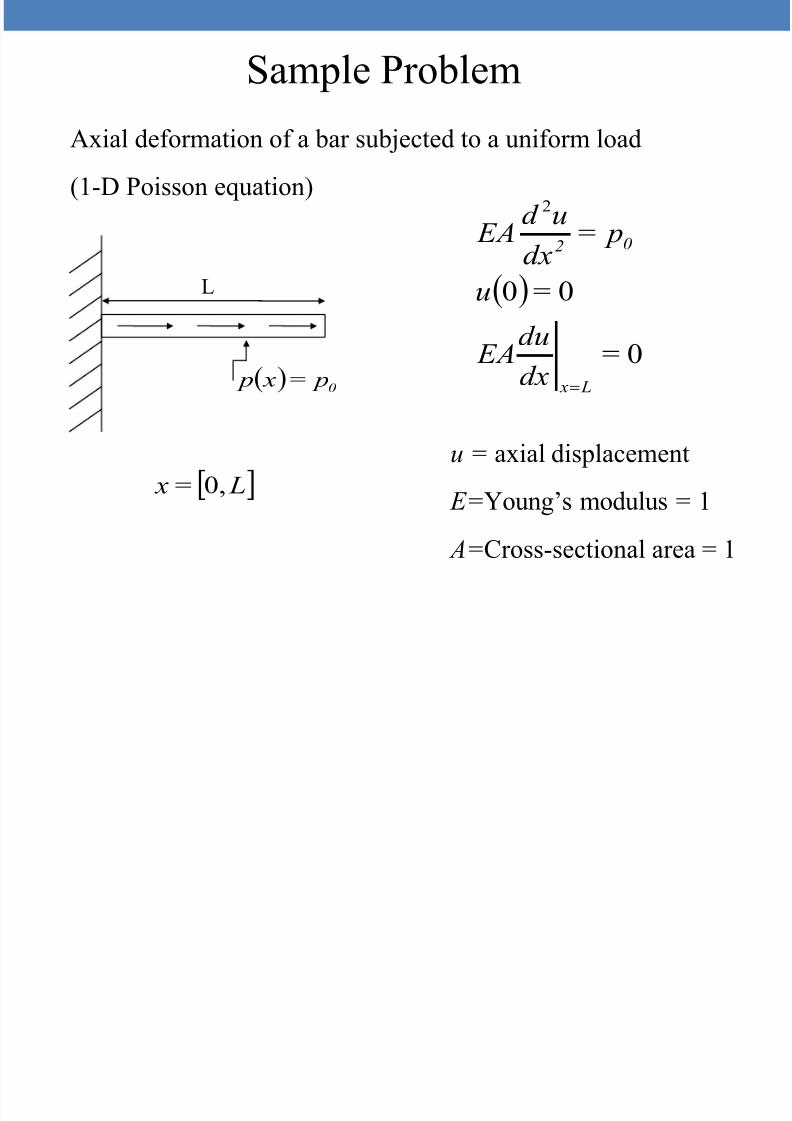
Axial deformation of a bar subjected to a uniform load

(1-D Poisson equation)

Sample Problem

0 p= x p

0

00

2

=dxdu

EA

=u

p=dx

ud EA

L x

02

L

L= x 0,u = axial displacement

E= Young’s modulus = 1

A= Cross-sectional area = 1



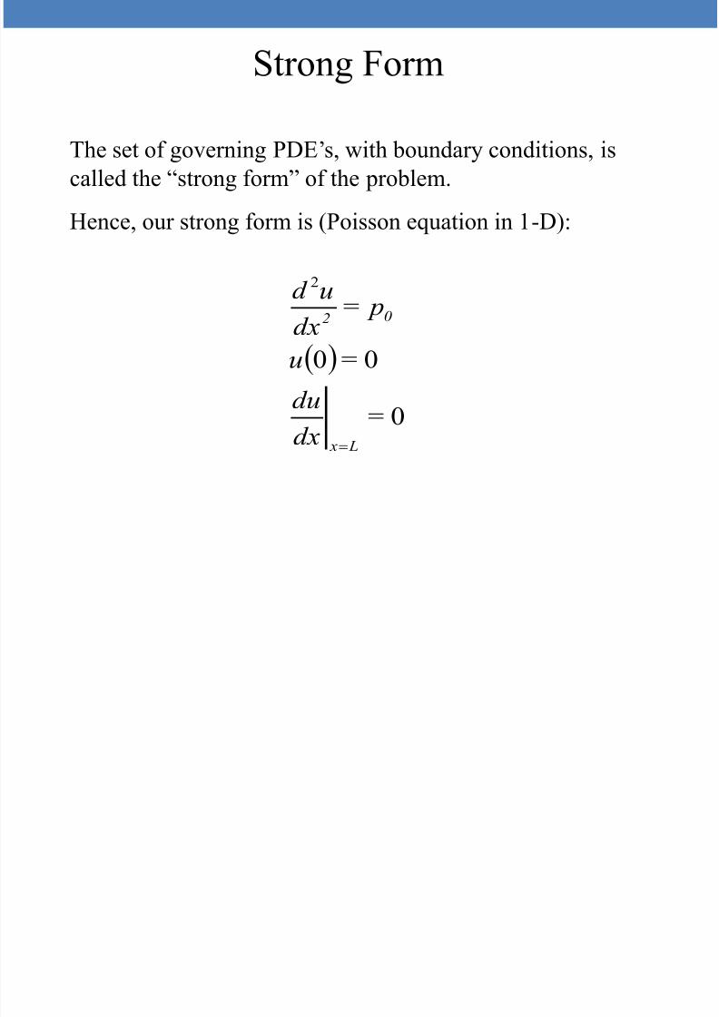
Strong Form

The set of governing PDE’s, with boundary conditions, iscalled the “strong form” of the problem.

Hence, our strong form is (Poisson equation in 1-D):

0

00

2

=dxdu

=u

p=dx

ud

L x

02



We now reformulate the problem into the weak form.The weak form is a variational statement of the problem inwhich we integrate against a test function . The choice of testfunction is up to us.

This has the effect of relaxing the problem; instead of findingan exact solution everywhere, we are finding a solution thatsatisfies the strong form on average over the domain.

Weak Form



Weak Form

0

0

0

0

2

0

2

2

=vdx pdx

ud = pdx

ud

p=dx

ud

L

2

2

02

Strong Form

ResidualR

=0

Weak Form

v is our test function

We will choose the test function later.



Why is it “weak”?

It is a weaker statement of the problem.

A solution of the strong form will also satisfy the weak form,

but not vice versa.Analogous to “weak” and “strong” convergence:

Weak Form

f x f x f

x x

n

n

lim :weak

lim :strong

n

n



Weak Form

Choosing the test function:

We can choose any v we want, so let's choose v such that itsatisfies homogeneous boundary conditions wherever the actual

solution satisfies Dirichlet boundary conditions. We’ll see whythis helps us, and later will do it with more mathematical rigor.

So in our example, u(0)= 0 so let v(0)= 0.



Returning to the weak form:

L L

2

L

2

vdx p=vdxdx

ud

=vdx pdx

ud

0 0

0

2

0

0

2

0

00

00

0

)(

x L x

L

L x

x

L

dx

duv

dx

du Lvdx

dx

dv

dx

du

dxdu xvdx

dxdv

dxdu

Weak Form

IntegrateIntegrate LHS by parts:



Weak Form

Recall the boundary conditions on u and v:

0)0(

0

00

v

=dx

du

=u

L x

L L

x L x

L

vdx pdxdx

dv

dx

du

dxduv

dxdu Lvdx

dxdv

dxdu

0 0

0

00

0

HHence,The weak form

satisfies Neumannconditionsautomatically!



Weak Form

functionallineara,functional bilineara

)(,such thatFind

:statementlVariationa10

1

0 0

0

F B

H vv F vu B H u

vdx p=dxdx

dv

dx

du L L

Why is it “variational”?

u and v are functions from an infinite-dimensionalfunction space H



We still haven’t done the “finite element method” yet, we have just restated the problem in the weak formulation.

So what makes it “finite elements”?

Solving the problem locally on elements

Finite-dimensional approximation to an infinite- dimensionalspace → Galerkin’s Method

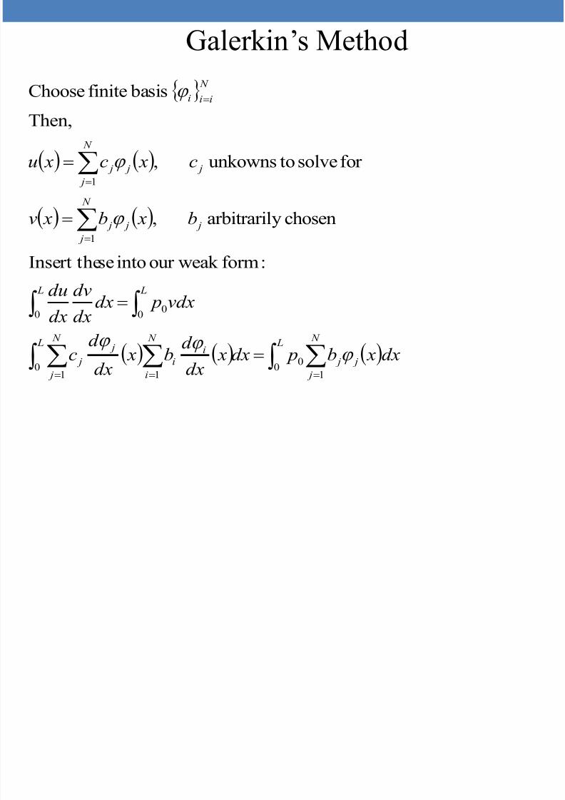
Galerkin’s Method



L N

j

L N

j j j

N

i

ii

j j

L L

j

N

j j j

j

N

j j j

N

iii

dx xb pdx xdx

d b x

dx

d c

vdx pdxdxdv

dxdu

b xb xv

c xc xu

01

01

01

0 0 0

1

1

:formour weakintoseInsert the

chosenyarbitraril ,

for solvetounkowns ,

Then, basisfiniteChoose

Galerkin’s Method



dx pdxdx

d

dx

d c

dx pbdxdx

d

dx

d cb

dx xb pdx xdx

d b x

dx

d c

i

L N

j

Li j

j

i

L N

ii

N

i

N

j

Li j

ji

L N

j

L N

j j j

N

i

ii

j j

0 01

0

0 011 1

0

01

01

01

:Cancelling

:gRearrangin

Galerkin’s Method



effect.without,einterchang

canwesincesymmetric bewillseealreadycanWe

and

,unknowns,of vectorais

where, problemmatrixahavenowWe

0 0

0

0 01

0

ji

K

dx p F

dxdx

d

dx

d K

c

dx pdxdx

d dx

d c

ij

i

L

i

Li j

ij

j

i L

N

j

L i j j

FKc

Galerkin’s Method



Galerkin’s Method

So what have we done so far?1) Reformulated the problem in the weak form.

2) Chosen a finite-dimensional approximation to the solution.

Recall weak form written in terms of residual:

00 00 02

2

L

i

L

ii

Ldxbvdxvdx p

dx

ud R R

This is an L2 inner-product. Therefore, the residual is orthogonalto our space of basis functions. “Orthogonality Condition”



Orthogonality Condition

00 00 02

2

L

i

L

ii

L

dxbvdxvdx pdx

ud R R

The residual is orthogonal to our space of basis functions:

u

uh

H

H h φ i

Therefore, given some space of approximate functions H h, we arefinding uh that is closest (as measured by the L2 inner product) tothe actual solution u.



Discretization and Basis Functions

Let’s continue with our sample problem. Now we discretize ourdomain. For this example, we will discretize x= [0, L] into 2“elements”.

0 h 2h=L

1Ω

2Ω

In 1-D, elements are segments. In 2-D, they are triangles, tetrads,etc. In 3-D, they are solids, such as tetrahedra. We will solve theGalerkin problem on each element.





Discretization and Basis Functions

To save time, we can throw out φ 1 a priori because, since in thisexample u(0)= 0, we know that the coefficent c1 must be 0.

x1= 0 x2=L/ 2 x3=L

φ 2 φ 3



Basis Functions

otherwise 0

,if 12

otherwise 0

,if 2

2

,0if 2

23

2

2

2

L x L

x

L x

L

x

x L x

L

L

L

x1= 0 x2=L/ 2 x3=L

φ 2 φ 3



Matrix Formulation

expected.assymmetricis Notice

s. polynomialfor

exactisitsince,quadratureGaussianusetoFEMinstandardisIt

.quadrature byynumericall performed ben wouldintegratio

andknown,arefunctions basisthesinceadvance,indone

becanfunctions basistheatingdifferenticode,computeraIn

,22

241

:haveweintegrals,theevaluatingthenfunctions,

basistheatingDifferenti problem.algebralinearaatarrive

andslide previouson thechoseninsert thecanWe

: problemmatrixourGiven

41

21

0

0 01

0

K

FK

FKc

FKc

FK c

L

p

L

dx pdxdx

d dx

d c

i

i

L N

j

Li j

j



Solution

2

:is problemfor thissolutionanalyticalexactThe

,nwhe)(

,0nwhe

:solutionnumericalfinalour

givesfunctions basis bymultipliedenwhich wh,

:tscoefficienourobtainwe

slide, previouson the problemneliminatioGaussiantheSolving

20

0

22

041

2043

2

83

20

20

x p Lx p xu

L x Lx L p

x Lx p x

c

L

L

i L p

L p

i

c



Solution

0

0.1

0.2

0.3

0.4

0.5

0.6

0 0 . 2

0 . 4

0 . 6

0 . 8 1

x

u ( x

) ExactApprox

Notice the numerical solution is “interpolatory”, or nodally exact.



Concluding Remarks

•Because basis functions are compact, matrixK

is typicallytridiagonal or otherwise sparse, which allows for fast solvers thattake advantage of the structure (regular Gaussian elimination isO( N 3), where N is number of elements!). Memory requirementsare also reduced.

•Continuity between elements not required. “DiscontinuousGalerkin” Method



THANK YOU

Documents

Pert 1 Introduction to Finite Element Methods