Embed Size (px)
Citation preview

COMPUTER METHODS IN APPLIED MECHANICS AND ENGINEERING 45 (1984) 28.5-312 NORTH-HOLLAND
FINITE ELEMENT METHODS FOR LINEAR HYPERBOLIC PROBLEMS
Claes JOHNSON Department of Mathematics, Chalmers University of Technology, S-412 96 Giireborg, Sweden
. . Uno NAVERT
Flygdivisionen Saab-Scania. S-582 66 Linkiiping, Sweden
Juhani PITKARANTA Department of Mathema~cs, Helsinki Uniz)ers~ty of Technology, SF-02150 Esbo 15, ~i~lan~~
Received 6 December 1982 Revised manuscript received 15 March 1983
We give a survey of some recent work by the authors on finite element methods for convection- diffusion problems and first-order linear hyperbolic problems.
0. Introduction
The purpose of this paper is to give a survey of some recent work on finite element methods for convection~iffusion problems and first-order linear hyperbolic problems by the authors [9-13, 171. The present paper is an elaboration of [lo].
We shall first consider a stationary scalar linear convection-dominated convection-diffusion problem of the form
-shuip*Vu+cru=f inft,
(0.1) u=g on r,
where 0 is a bounded domain in RN with boundary r, p = (&, . . . , &) and a are smoothly varying coefficients with IpI - 1 and E >O is a small constant. The solution u of this problem is in general not globally smooth even for smooth data f and g [20]; in general u will vary rapidly in a layer of width O(E) at the outflow boundary r+ = {x E T: n(x) * /3(x) 30) where n(x) is the outward unit normal to r at x E f. Moreover, in the limit case E = 0 where the boundary data g are only prescribed on the inflow boundary r... = {x E r: n(x) * /3(x) < 0} u will be discontinuous across the characteristic curve (streamline) x(s) given by dxfds = p(x), x(O) = x0 E r_, if e.g. g is discontinuous at x 0. If E > 0 then such a discontinuity is spread out over a layer around the characteristic x(s) of width O(~E).
A ‘classical’ problem in numerical analysis is to construct, using a mesh with mesh length h not oriented to follow the characteristics, a finite difference or finite element method for (0.1) that (i) is higher-order accurate and (ii) has good stability properties without requiring h to be smaller than E. Conventional schemes for (0.1) fall into one of the following two categories
00457825/84/$3.00 @ 1984, Elsevier Science Publishers B.V. (North-Holland)
2Xh C. Johnson et al., FEM for hyperbolic problems
each one satisfying only one of the above conditions. The first class of methods consists of formally higher-order accurate methods such as e.g. the standard Galerkin method (see below) or finite difference methods based on using centered difference approximations for the convective term p . Vu. These methods will produce severely oscillating approximate solutions
unless h < E or the exact solution happens to be globally smooth. In the other class we find the classical monotone upwind schemes obtained by adding an artificial diffusion (or viscosity) term of the form -h Au. These methods satisfy (ii) and produce non-oscillating approximate solutions but are only first-order accurate being based on solving a modified problem.
Note that we do not assume that the mesh matches the characteristics of (0.1) so that in particular the same mesh may be used for different flowfields p. If the mesh is oriented to follow the characteristics, we get methods with qualitatively different properties which may be considered to be variants of the method of characteristics.
We shall in Section 1 consider a finite element method for (O.l), the streamline dijfusion method introduced by Hughes and Brooks [2, 5, 61 which satisfies both the conditions (i) and (ii) stated above. This method is a Petrov-Galerkin modification of the standard Galerkin method where artificial diffusion in the streamline direction is introduced by modifying the test functions from u to u + hp * Vv. The mathematical analysis of this method was started in [9] and was carried further in [ 171. The main results in [17] concerning the streamline diffusion method for (0.1) are roughly speaking the following if F < h and piecewise polynomials of degree k are used. Here uh denotes the finite element solution.
(A) Global error estimates.
(0.2)
where
lllwllln = ~/rllVwllL*cn, + -\/QP * WlL2u2~ + II42V2~
and H”(R) for s a positive integer denotes the usual Sobolev space with norm 11. IIHyRj. We note that this is an improvement of the corresponding estimate for the standard Galerkin method which reads
(0.3)
Notice in particular the presence of the term X&II/~ . V(u - ~~~~~~~~~~~ on the left-hand side of (0.2), which means that the streamline diffusion method has an improved stability for the streamline derivative /3 * V as compared to the standard Galerkin method.
(B) Localization results. These results state that effects are propagated in the discrete problem approximately as in the continuous problem, i.e. approximately along the charac- teristics. More precisely it is proved that the influence of a source in the discrete problem decays with the distance d to the source like exp(-Cd/h)_ in any direction with a positive
component in the upwind direction -p and like exp(-Cd/d\/) in directions orthogonal to the
streamlines (crosswind directions). Alternatively, these results can be phrased as local error estimates of the form
lllu - UhlllR'~ Chk+“2tllulI~~+1cn,,,+ llfIIw,+ kbd (0.3)
C. Johnson et al., FEM for hyperbolic probietns 287
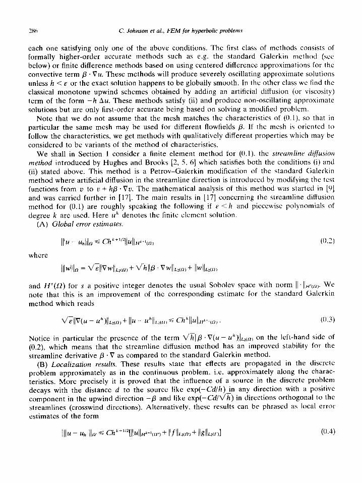
where a’ C W, the distance_from a point x E a’ to 0\0” is O(h log l/h) in directions not orthogonal to p and O(gh log l/h) in crosswind directions. Moreover 0” satisfies the following condition: if f E 0” then all points x = 2 - $3 with s > 0 belonging to fl also belong to KY’, i.e., all points upstream a point in 0” also belong to a”, or in other words, a“ does not allow ‘upstream cut-off’ (see Fig. 1).
Note that the standard Galerkin method for (0.1) does not allow such local estimates; in fact in this case effects may propagate in crosswind or even upwind directions with little damping. Previously, local error estimates for finite element methods have been proved only for elliptic [16] and parabolic [l9) problems. The essential tool in all these localization results including the hyperbolic case considered here is the super-approximation lemma by Nitsche and Schatz [16]. For (dissipative) finite difference methods for linear hyperbolic problems localization results were proved by Fourier methods in e.g. [l].
In Section 1 we give proofs of the results (A) and (B) under some simplifying assumptions. In Section 2 we present results analogous to (A) and (B) for the discontinuous Galerkin
method for (0.1) with E = 0 (see [12]). This improves in particular earlier global error estimates by Lesaint-Raviart [14]. We also state &-estimates, 1 sp s ~0, for the model problem u, = 0 in 0, u = g on r_, with /3 constant, obtained by Fourier methods in the case of regular meshes with piecewise linear or piecewise constant trial functions [12]. In the piecewise linear case one may with a proper interpretation view the discontinuous Galerkin method as a non-standard difference scheme which is accurate of order 3 and dissipative of order 4, while in the case of piecewise constants the discontinuous Galerkin is a variant of the usual upwind finite difference scheme which is accurate of order 1 and dissipative of order 2.
In Section 3 we present an extension of the streamline diffusion method to the time-
Fig. 1.
28X C. Johnson et al., FEM for hyperbolic problems
dependent problem (see [ 171)
u,-~1u+p~Vu+cvr~=f in RX(O,T).
II = g on I’ X (0, 7) ,
II = U() in R for t = 0.
(0.5)
where ~4, = &4/i% and now p and (Y are smooth functions of (x, t). This method is based on using space-time elements with the trial functions being continuous in space and discontinuous in time. Again results analogous to (A) and (B) are valid, i.e., the method combines high accuracy with good stability. However, the resulting scheme is implicit (on each time level one has to solve a linear system of equations) and thus for this scheme to be really useful in
practice it should be possible to solve the (non-symmetric) system of equations at a reasonably low cost. Using a localization result we demonstrate that it is in fact possible to solve this system with sufficient accuracy with O(KN[log l/hlN) operations in the case of constant coefficients and O(KN[log l/h]“N) operations in the case of variable coefficients, with a = 2 if N = 2 and a - 2.33 if N = 3, by replacing the given implicit scheme by an explicit scheme involving O(log l/h) points in each coordinate direction. Thus, at least asymptotically the operation count for this method as compared with an explicit method requiring O(h -N ) operations does not appear to be prohibitive. Of course the magnitude of the constants involved in these estimates is crucial and more numerical experiments than presently available are needed to evaluate the practical usefulness of the indicated procedure.
In Section 4 we consider extensions of the streamline diffusion method to Friedrichs’ systems and we present results analogous to (A) and (B). In this case the localization result states that the cone of dependence in the discrete problem is a close approximation of the cone of dependence in the continuous problem. Similar results are also given for the discontinuous Galerkin method (see [13]).
To sum up, it seems that starting from the streamline diffusion method for the stationary convection-diffusion problem (0.1) one may construct finite element methods for a large class of linear hyperbolic problems which are higher-order accurate and have good stability properties. The analysis presented below shows the need of using a more precise stability concept for numerical methods for linear hyperbolic problems than that used in the classical analysis of e.g. finite difference methods or the standard Galerkin method. In this latter classical approach one only uses L,- (or possibly L,-) stability results of the form
Ildiscrete solutio&, c C/datallrZ .
which typically lead to non-optimal error estimates of the form (0.3) and which do not admit localization. This seems to be analogous to the situation for elliptic (and parabolic) problems for which the usual finite element method has excellent stability properties resulting in optimal error estimates of the form
Ilerro&_, S Ch ‘+‘ljexact solutio&~+~ ,
whereas the classical finite difference analysis based on e.g. maximum principles leads to
C. Johnson et al., FEM for hyperbolic problems 289
severely non-optimal error estimates. If we agree to say that the ‘gap’ of a numerical method allowing an error estimate of the form
Ilerror]],, s Ch”(Jexact solutio&~
is equal to r - s, then we may say that the standard Galerkin method as well as finite difference methods for linear hyperbolic problems (according to the classical theory) have gap = 1 while the gap of the streamline diffusion method is f. For elliptic problems the usual finite element methods have zero gap.
Let us conclude this section by briefly commenting on some applications and possible extensions together with some open problems. In [ll] the improved estimates for the discontinuous Galerkin method mentioned above are used to analyze a fully discrete method for a stationary neutron transport problem in two space dimensions based on using the discrete ordinates method for the angular variable and the discontinuous Galerkin with piecewise linear trial functions for the space variable. Previous convergence results for fully discrete schemes for neutron transport have been limited to the case of one space dimension. Applications of the discontinuous Galerkin method to other problems in transport theory are conceivable. Extensions of the theory to semi-linear hyperbolic problems may also be possible. In the work by Hughes and Brooks [5, 61 and Hughes, Tezduyar and Brooks [7] the streamline diffusion method is applied to Navier-Stokes equations and hyperbolic conservation laws and the results of several successful numerical experiments are reported. No doubt it is a challenging mathematical problem to analyze procedures of this type. Another open problem is to prove &,-error estimates for linear problems in the case of general meshes. L,-estimates with gap f can be proved by Fourier methods (see [12] and Section 2) for regular or piecewise regular meshes. From the weighted &-estimates to be presented below one may derive some &-estimates with gap > 1 for general meshes but these estimates may not be optimal.
For results of numerical experiments we refer to [17] for the methods of Sections 1 and 3.
1. The streamline diffusion method for a stationary convection-diffusion problem
1.1. Preliminaries
We shall consider the problem (0.1) i.e.,
-cAu+p*Vu+au=f ina,
u=g on r,
together with the corresponding reduced problem with E = 0,
p*Vui-au=f ina,
u=g on r_ .
(1.1)
(1.2)
We shall for simplicity assume 0 to be a polygonal domain in W*. Moreover we shall assume
29( )
that
C. Johnson et al.. FEM for hyperbolic problems
(T - i div p 3 6 in f2 (1.3)
where a is a positive constant. The condition (1.3) can be relaxed if the flow field /3 contains no closed streamlines; it is then sufficient to require the constant (T to satisfy u > 6(&) where C(E) is a certain function of F such that (T(E) += --x as E + 0. In particular, if F = 0 then (1.3) is not needed in this case (since (T and p are smooth, u - f div /? is bounded below on 0).
We shall below use the following notation:
Vu+Vwdx,
(v, w> = 1 vwnspds, I‘
(u, w)-=I vwn.pds, (u, w), = 1 uw n . p ds , r- I’*
where f_ = {x E r: n(x). p(x) CO} and r+ = I-\E. Note that by Green’s formula we have
(~8, w) = (a w)- (u, wP)- (v, w div p) . (1.4)
By C and c we will denote positive constants independent of h, E, u and the data f and g, not necessarily the same at each occurrence.
Let now {Th} be a family of triangulations Th = {K} of 0, satisfying as usual the minimum angle condition (see [3)), and indexed by the parameter h representing the maximum diameter of the triangles K E Th. For simplicity we shall below assume that {T,,} is quasi-uniform, i.e., there exists a constant c such that the length of any side of a triangle K E Th is bounded below by ch (cf. Remark 1.4). For a given positive integer k we introduce the finite element space
Vh = {v E H’(a): & E P,(K) WC E Th} (1.5)
where Pk(K) is the set of polynomials on K of degree less than or equal to k, i.e., V,, is the space of continuous piecewise polynomial functions of degree k. By the usual approximation theory we have [3]: Given a function u E H ‘+‘(a) there exists an interpolant tih E Vh such
C. Johnson et al., FEM for hyperbolic problems 291
that
(1.6a)
(1.6b)
Let us before presenting the streamline diffusion method first recall the standard Galerkin method and the classical artificial diffusion method.
1.2. Standard Galerkin method
Let us first consider the full problem (1.1) and let us then for simplicity assume that the boundary data g is equal to zero. The standard Galerkin method for this problem with strongly imposed boundary conditions reads: Find uh E e,, = {u E vh: 2, = 0 on r} such that
&(Vr& Vu)+ (u; + u.Uh, v) = (f, u) tl 2) E v,, . (1.7)
For the reduced problem (1.2) the standard Galerkin method with weakly imposed boundary conditions reads: Find uh E v,, such that
For methods (1.8) and (1.7) with E c h it is possible to prove the following error estimate,
IIu - uhll + Iu - uhl s Chkllull,‘+l . (1.9)
This estimate is a consequence of (1.6) and the following stability property of the bilinear form given by (1.8):
(w)9+uw,w)-(w, w)-Gllwl~+$Iw12 VwEH’(R), (1.10)
which follows from (1.3) and (1.4). In problem (1.7) we have an additional term e[lVwl~ but since E may be arbitrarily small we cannot rely on this term for the stability. Thus, only L,-stability is guaranteed. As noted above, the standard Galerkin method does not perform satisfactorily if the exact solution is non-smooth.
1.3. Classical artificial diffusion method
For problem (1.1) with g = 0 this method reads if E C h: Find uh E e,, such that
h(Vuh,Vu)+ (U;+uUh,2))=(f, U) VvE eh.
This method has good stability properties due to the presence of the term h(Vuh, Vu) for all E > 0 but the method is at most first-order accurate, i.e., the error is at best O(h).
We now come to the main topic of this section.
‘0’ _- C. Johnson et al., FEM for hyperbolic problems
1.4. The streamline difiusion method
It turns out that to eliminate the oscillations in the standard Galerkin method in the case E < h it is sufficient to add a term - hupp i.e., a diffusion term acting only in the direction of the streamlines. Such a modified artificial diffusion method for (1.1) would read: Find 14~ E I/,,
such that
&(vUh, VU)+ h(u;, U,)+ (u; + guh, U)’ (f, U) t/ U E o/h. (1.11)
This method introduces less crosswind diffusion than the classical artificial diffusion method
but still corresponds to a modification of the original problem (this method is similar to a finite difference method proposed in [ZS]). However, it is possible to introduce the crucial term h(ui, va) appearing in (1.11) without such a modification. Let us first see how this can be done
in the case E = 0.
1.4.1. The streamline diffusion method with E = 0
Let us start from the standard Galerkin method (1.8) with weakly imposed boundary conditions. If we in the terms (a, *) replace the test function u E V, by v + hv,, we get the streamline diffusion method: Find uh E vh such that
(u; + uuh, u+hu,)-(uh,u)-=(f,U+h~~)-(g,u)_ YUE v,. (1.12)
We notice here the presence of the term h(ui, up). Further, we notice that relation (1.12) is valid also if we replace ~4~ by the solution u of (1.2) i.e., method (1.12) is not based on a modified
problem. Let us now analyze method (1.12) and let us then introduce the following notation,
B(w, u) = (wp + uw, u + hup)- (WY v>- , L(u) = (f, u + hu,)- (8, v>- .
By (1.2) and (1.12) we have the following error equation with e = u - uh,
B(e,v)=O VuE V,. (1.13)
(A) A global error estimate. We shall now prove a global error estimate in the following norm,
This choice of norm is related to the following stability property of the bilinear form B which again follows from (1.3) and (1.4): For any v E HI(o) we have for h small enough
WA u> z= cll14112 . (1.14)
Notice that the form B has an improved stability as compared with the bilinear form associated with the standard Galerkin method (1.8) satisfying (1.10). From (1.14) we obtain
using Cauchy’s inequality
C, Johnson et al., FEM for hyperbolic problems 293
the following a priori estimate: If uh E vh satisfies (1.12) then
Id> * (1.15)
In particular this estimate shows uniqueness and hence also existence of a solution to (1.12). We can now state and prove the basic global error estimate for (1.12)
THEOREM 1.1. If uh satisfies (1.12) and u satisfies (1.2), then
l\lU - Uhlll s Chk+1’211Uljk+1 . (1.16)
PROOF. Let r?’ E vh be an interpolant of u satisfying (1.6). Writing qh = u - Uh and eh = Uh - Uh, and using (1.14) with u = e and (1.13) with v = eh, we get for h $4,
clllell12 d B(e, e) = B(e, qh)- B(e, eh)= Bk rlh) = (ep, qh)+ h(e,, vi)+ (ae, qh)+ h(ae, r)i)-_(e, rlh)-
&h Ijes\r + Ch-‘llrl hll2 + achlleplr + ChJ[qi1(2+ b?IleIl2 + Chhll + $c6llelr+ Ch*((qi(r+ &xl*+ CIqh12.
Recalling the approximation result (1.6) we thus have
lllelll* d Ch2k+111ul12k+l ,
which proves the desired estimate.
(B) Localization results. We shall next prove an analogue of the stability estimate (1.15) in a weighted norm from which the localization results stated in Section 0 may be derived. For simplicity we shall then consider the case /3 constant with IpI = 1 and assume k = 1, i.e., we shall assume that vh consists of continuous piecewise linear functions (for p variable and k 3 1, see [17]).
We shall first consider weight functions I/J(X) of the form
w = (P(V) where 8 E IX* is a unit vector such that
p*e>o,
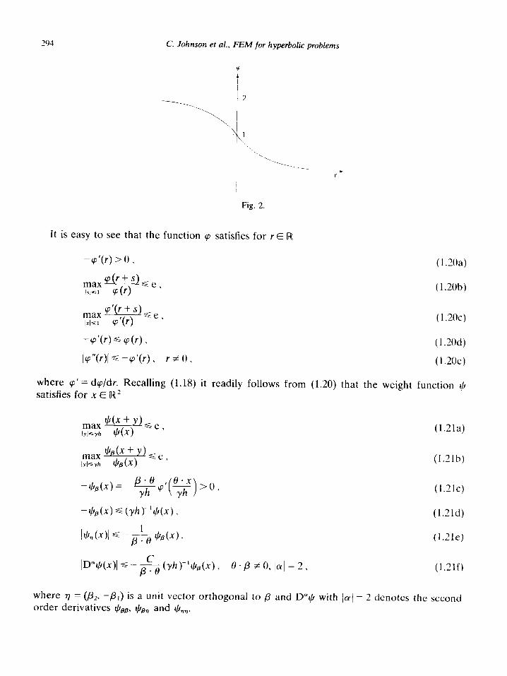
and 40 : R + R is the following cut-off function with exponential decay (see Fig. 2)
(1.17)
(1.18)
(1.19)
and y is a positive constant to be chosen sufficiently large as specified below.
C. Johnson et al., FEM for hyperbolic problems
Fig. 2.
It is easy to see that the function cp satisfies for r E R
-q’(r) b-0, (1 Xa)
( 1 .ZOb)
(1.2(k)
-cp’(r) s 4-1 1 (1.2Od)
Iq”(r)lC-q’(r), rf0, (I .2Oe)
where cp’ = dqldr. Recalling (1.18) it readily follows from (1.20) that the weight function $ satisfies for x E R2
(1.21a)
(1.21b)
(l.Zlc)
-h?(x) d wccl,(~) * (1.21d)
lM~-~W. (1.21e)
ID”W)l d - &j (yWllrp(4 3 &p7qcl=2, (1.21f)
where 7 = (,&, - order derivatives’;)
IS a unit vector orthogonal to ,!? and D”+ with /LY/ = 2 denotes the second
PP? +%J and &lT
C. Johnson et al., FEM for hyperbolic problems 295
We shall prove the following weighted a priori estimate where for w a non-negative weight function we use the following notation:
I{ 011, = (I, V%J dx)“* , Iv/, = (I, v*ln -Plu ds)“*, Illulll* = (~llv~ll~+ Il4l%-J1,,*+ %J13’n +
THEOREM 1.2. Suppose that $ satisfies (1.21). If y is sufficiently large there is a constant C such that if w E V, and
then ~(w,v)=(f,v+hv~) VVE V,,
lIMlI* d CllfllJI *
(1.22)
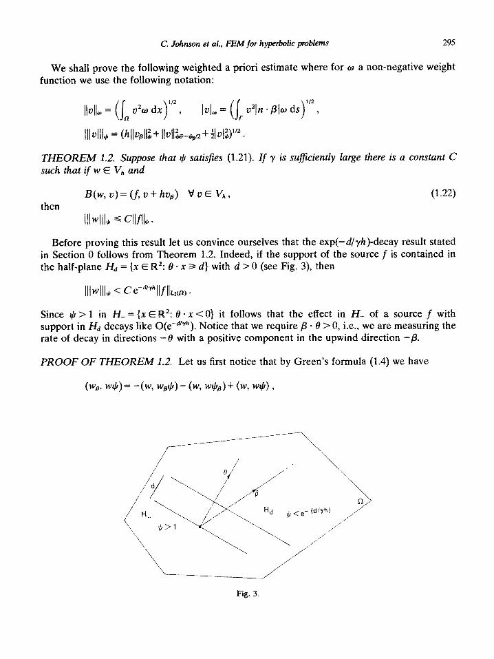
Before proving this result let us convince ourselves that the exp(-d/yh)-decay result stated in Section 0 follows from Theorem 1.2. Indeed, if the support of the source f is contained in the half-plane Hd = (X E W2: 0 - x 2 d) with d > 0 (see Fig. 3) then
Since $I > 1 in H_ = (X E R2: 8 -x < 0) it follows that the effect in I-I_ of a source f with support in I& decays like O(eTayh ). Notice that we require /3 - 6 > 0, i.e., we are measuring the rate of decay in directions -8 with a positive component in the upwind direction -p.
PROOF OF THEOREM 1.2. Let us first notice that by Green’s formula (1.4) we have
Fig. 3.
296 C. Johnson et al., FEM for hyperbolic problems
so that B(w, w$) = (wg, w$) + (gw, w+) + +Q3, (w$)a) + h(~W, (w+Q3) - (w, w$‘)
= $lwl$+ lilwIl~~P + IIwll;Q + hllw&+ wQ7 w&3)+ h(aw, (wfl)P) 2 IllwIll;+ M&v wtcls) + ww bwP>~
Now, by (1.21d) we have
lwp, w$)I ~4~*llW,lIZ-~~ + QIMI’~~
d 4~r-111w,ll:+ illWll’tiB .
Hence, using similar estimates for the remaining term h(aw, (wI,!J)~) it follows that if y is large enough, then there is a positive constant C such that
NW WV B clllwlll:, . (1.23)
On the other hand, by (1.22) we have, with (w$)~ E V,, denoting the usual interpolant of WIJ interpolating w$ at the nodes of Th,
B(w, WlcI) = B( w, w+ - (W@)h) + (J (W$)h + 4+M.
Let us here first consider the term (wp, w$ - (w+),,) included (w$),,). We have
(1.24)
in the expression B( w. w$ -
(1.25)
Now, by the analogue of the approximation result (1.6a) for one triangle K together with (1.21a) we find after summation over K
so that, since w is linear on each K,
We shall now estimate the terms on the right-hand side of this inequality. First, by (1.21d) we have
(1.27)
C. Johnson et al., FEM for hyperbolic problems 297
Next, recalling the inverse estimate (cf. [3])
]]Vv]]MW s Ch-l(jv(jL~(K) v 2, E PI(K) ,
and using (1.21b), we see that
Also, by (1.21e),
IIw,+,b,Jl$-: + IIwpt,b,J~-~ s Ch-2 I, w2@-‘dx s Cy-‘h-3~~w~~2-, .
Finally, by (1.21f),
, z2 lbDVll31~ Ch-211wh&-~ s W1h-311wl12-~~ a
(1.28)
(1.29)
(1.30)
(1.31)
Combining now (1.26)-(1.31) we find that for y 2 1
lb+ - bwhll~-~ d CY-1’2h’n(h”211wslle + llwll-+,> 9 (1.32)
so that by (1.25)
Ih.3, w - (WM s w’“lll4ll:~ (1.33)
The remaining terms in B(w, wr,G - (w$),,) can be bounded similarly and thus by (1.23) (1.24) and (1.33) we have if y is sufficiently large
~~b~~~~~ c(f, cw+)h + h(“@h,) = c[(f, w$l> + W (WV%) + (h tw+cI)h - W’b) + U (w+hB - k/%)1
from which follows, by the same type of arguments as used above,
This completes the proof.
REMARK 1.3. The estimate (1.32) may be considered to be the analogue in the present context of the Nitsche-Schatz super-approximation lemma [16].
Let us now give a result on the rate of decay in the crosswind direction rl satisfying
2% C. Johnson et al., FEM for hyperbolic problems
r] . p = 0. In th is case we choose the weight function (Ir as follows:
(1.34)
Note that in this case $D = 0 and therefore we cannot take advantage of estimates of the form
(1.21d), (1.21f) as was done in the proof of Theorem 1.2. From (1.34) it follows that $ satisfies again (1.21a), (1.21b) and
Using these estimates and following the proof of Theorem 1.2 we easily find a result analogous to Theorem 1.2 with $ now given by (1.34). This result states that effects decay in the crosswind direction with the distance d at least as rapid as O(exp(-d/yd/h)).
REMARK 1.4. The assumption that {Th} is quasi-uniform is not essential. If {r,,} is not quasi-uniform then (1.12) is generalized as follows:
@+ouh, u+ 8Up)-(Uh, v)_ = (h v+ 6vp)-(g, v)_ V u E v, (1.36)
where now
6 = hK = diameter of K on K
Theorem 1.1 naturally extends to this case. The localization results can also be extended to this case if {Th} is locally quasi-uniform or more precisely if there is a smooth function H(x) and positive constants c and C such that
chH(x)sh,sChH(x), XEK,
In the case of Theorem 1.2 the weight function $ is then defined as follows
and correspondingly for the crosswind decay result.
REMARK 1.5. As indicated above one may relax condition (1.3) if E is small. If F = 0 and /? constant let 6 be the minimum of (T over R. The desired stability of the discrete problem including the control of the &-norm follows in this case from Theorem 1.2 by choosing the weight function
CW = p$ exp(-W + ld>P * XMW
C. Johnson et al., FEM for hyperbolic problems 299
with $ as above. We have
and the L,-stability follows from the presence of the term 1) - \1+&d2 in the norm 1)) - )I)$.
REMARK 1.6. For a flow field /3 with more general variation not necessarily satisfying I/3] - 1, the streamline diffusion method for (1.2) takes the form (1.36) with
6=0 otherwise,
where PK E K. If 5 > 0, then the above analysis can be carried out without assuming I@(x)] to be bounded away from zero and thus in this case the presence of stagnation points where I/~(X)] = 0 does not present any difficulties.
1.4.2. The streamline diffusion method with E > 0 The generalization of the streamline diffusion method (1.12) to the full problem (1.1) with
g = 0 reads (cf. [6]): Find L? E ?‘,, such that
(1.37)
where S = ch if E 4 h with c sufficiently small, 6 = 0 if E 2 h, and for w, u E vh,
A wvsdx . (1.38)
Notice that by multiplying (1.1) by u + hv, it follows that (1.37) holds with uh replaced by U. The error estimate (1.16) and the localization results stated above for (1.12) can be extended to the method (1.37) with E <h (see [17]). T o sum up, (1.37) is an answer to the problem of finding a higher-order accurate method for (1.1) with good stability properties.
Let us here give a proof of the basic stability estimate for (1.37) in the case E < h which in particular proved that the presence of the term -&S(Auh, up) does not degrade the extra stability introduced by the term a(~;, up) if the constant c is small enough. By the inverse estimate (1.28) we have
so that, recalling (1.14)
300 C. Johnson et al., FEM for hyperbolic problems
Thus, if c is so small that
which proves the desired stability result.
REMARK 1.7. If {T,,} IS not quasi-uniform, then in (1.37) we choose 6 = chK on K.
2. The discontinuous Galerkin method
Galerkin methods for (1.1) and (1.2) based on using continuous trial functions will lead to globally coupled systems of linear equations, i.e., systems where a change in data at one node will affect the solution at all nodes. This is natural e.g. for the elliptic problem (1.1) with E > 0 but not so for the purely hyperbolic reduced problem (1.2) corresponding to F = 0. In the latter case it would be more natural to be able to solve the linear system by successive elimination starting at the inflow boundary r_.
We shall now consider a finite element method for the reduced problem (1.2) which permits such a solution procedure and which has convergence properties similar to the streamline diffusion method. This method, the discontinuous Galerkin method first studied by Lesaint- Raviart [14], is based on using the following finite element space:
w, ={uEL~(R):~(KEP~(K)~~KE Thl. (2.1)
i.e., the space of piecewise polynomials of degree k 2 0 with no continuity requirements across
interelement boundaries. To define this method let us first introduce some notations. For K E Th let us split the
boundary dK of the triangle K into an inflow part dK_ and on outflow part ilK+ defined by dK- = {x E dK: n(x). /? CO} and dK+ = dK\dK_ where H(X) is the outward unit normal to 3K at x E dK. Further, for a function u E W,, which may have a jump discontinuity across a side S common to two triangles K and K’, we define the left- and right-hand limits u- and U+ by
v_(x) = !\n$ u(x + sp) , u+(x) = hil u(x + sp>
for x E S and we also introduce the jump [II] across S defined by [II] = U+ - u_. The discontinuous Galerkin method for (1.2) can now be formulated as seeking a function
uh E W,, according to the following rule: For K E Th, given u!! on dK_ find uh = uhlK E Pk(K) such that
(u;; + alh, u + &)K -
V v E P,(K)
uh+u+n . p ds = (f, u + &)K - I
uhv+n . p ds 8K-
(2.2)
C. Johnson et al., FEM for hyperbolic problems 301
where ( * , + )K denotes the &inner product over K, u!! = g on I’_ and S = 0 or 6 = h. Note that for a given K (2.2) is nothing but the standard Galerkin method (1.8) if 6 = 0 and the streamline diffusion method (1.12) if 6 = h in the case of just one element. The method of Lesaint-Raviart corresponds to choosing S = 0 but it is natural to also consider the case 6 = h. Starting at r_ where u!! = g we can successively, triangle by triangle, determine uh in R from (2.2). For the solution U” of (2.2) one easily obtains the following stability estimate:
(2.3)
where x3, indicates summation over all sides S of Th, u$ = 0 on I’, and y1 is a unit normal to S. This estimate follows by choosing 21 = u h in (2.2) if 6 = h and v = uh + ChB * Vuh with C sufficiently small if 6 = 0. Here 6 is a piecewise constant approximation of /? e.g. defined by ,B = /3(PK) on K w h ere PK is the midpoint of K. From this stability estimate one can obtain an error estimate for the discontinuous Galerkin method analogous to Theorem 1.2. This improves earlier results by Lesaint-Raviart [14] who proved error estimates of the form IIu - ~~11 c Ch”llull k+l using only &-stability. One can also prove localization results analogous to those for the streamline diffusion method presented in Section 1.4.
If the triangulation TI, is uniform, /3 is constant and k = 0 or k = 1, then it is possible to analyze the method (2.2) as a finite difference scheme (if k = 0 then (2.2) reduces to essentially the usual upwind scheme which is accurate of order 1 and dissipative of order 2 whereas for k = 1 (2.2) corresponds to a non-standard difference scheme which is dissipative of order 4 and accurate of order 3 if f = 0). Using Fourier analysis one can in this case prove the following &,-generalization of the error estimate (0.2): There is a constant independent of p, h and u such that for 1 s p c 00,
Here Wy’(J2) is the usual Sobolev space of functions with derivatives up to the order k + 1 in I&2). One can further show that in the range 26~ 6 M estimate (2.4) remains valid if {Th} is a family of piecewise uniform triangulations, i.e., if each Th is obtained as a piecewise uniform refinement of a given coarse triangulation T.
For the results in this section we refer to [12].
3. The streamline diffusion method for a time-dependent convection-diffusion problem
3.1. The streamline diffusion method
Let us now consider the time-dependent problem (0.5) for simplicity with g = 0 and ty = 0, i.e., the problem
~~+z+-eA~=f inflx(O,T),
u=o on rx(O, T),
u = & in R for t = 0.
(3.1)
302 C. Johnson et al.. FEM for hyperbolic Froble~s
For E = 0 the corresponding problem with boundary data prescribed only on the inflow boundary r_ has the form (1.2) and the natural method to use is then the discontinuous Galerkin method. This would give a method with space-time elements. However, it is not clear how to generalize this method to the case I > 0; to handle the diffusion term --I Au the trial functions need to be continuous in the space variable. On the other hand to be able to compute the discrete solution successively on one time level after the other, it is natural, if we insist on using space-time elements, to use trial functions which are discontinuous in time. We are thus led to consider a method where the trial functions are continuous in space and discontinuous in time based on a triangulation of space-time with the elements organized in strips in time.
To define such a method let 0 = to < t, < * - - < tM = T be a subdivision of the time interval ((1, T) and introduce the strips S, defined by
s, = {(x, t): x E 0, t, -c t < tn+J
for n = 0, . . . , M - 1. Further, for each fz let V be a finite element subspace of Hi(&) based on a quasi-uniform finite element subdivision of the strip S,, with elements of size h > F and let V = (0 E V” : c(x, t) = 0 for .Y E I’}.
If we now apply the streamline diffusion method (1.12) successively on each strip to the problem (3.1), imposing the initial value at t = t, weakly and the boundary conditions strongly, we obtain the following method [lo, 171: For n = 0, . . . , M - 1, find U” E @ such that
(u: + u;, u-i- 6(u, + up))n 4 (u:. u,)!! + E(VU”, vu)” - &S(hU”, u* + up)” = = (fi u + 6(u, + II@))” + (U!!, u+)lt v u E ets. (3.21
where 6 = c/i if & < h. S = 0 if F 3 h, uli = u. = initial data,
(w, u)” = jsa wu dx dt,
u+(x, t) = lim u(x, t + s) , s-o+
u-(x, t) = KrJ u(x, t + s) I
and the last term on the left-hand side of (3.2) is defined as a sum over all elements in S, as in (1.38). For each ~1, (3.2) is equivalent to a linear system of equations and thus (3.2) is an ~~~~~c~~ scheme.
REMARK 3.1. The method (3.2) differs from the generalization of the streamline diffusion method (1.12) to time-dependent problems given in [2, 61, where finite difference methods are used for the time discretization. For t: = 0 it is not possible to distinguish between space and time in (3.1) and in this case it seems very natural to use space-time elements as is done in the discontinuous Galerkin method. Thus, for E small it seems reasonable to follow the same idea and use space-time elements also in this case. For E = 1 (and thus 8 = 0) the method (3.2) coincides with a method considered in IS],
C. Johnson et al., FEM for hyperbolic problems 303
For the method (3.2) with E < h and c sufficiently small one can prove results analogous to Theorems 1.1 and 1.2 (see [17]). Thus, (3.2) is a method for (3.1) which combines high accuracy with good stability. In the case of one space dimension, E = 0, and piecewise linear trial functions on a uniform mesh, (3.2) corresponds to a non-standard implicit finite difference method which is accurate of order 3 and dissipative of order 4, see [17] where also numerical results and comparisons with various difference methods are presented.
3.2. Approximate solution of the linear system on each time level
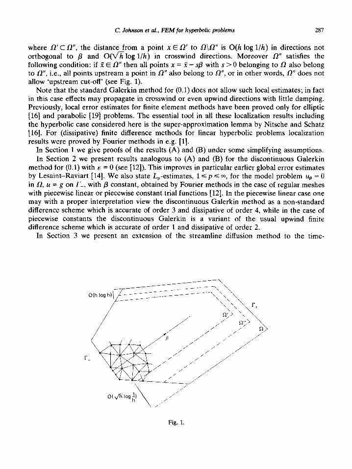
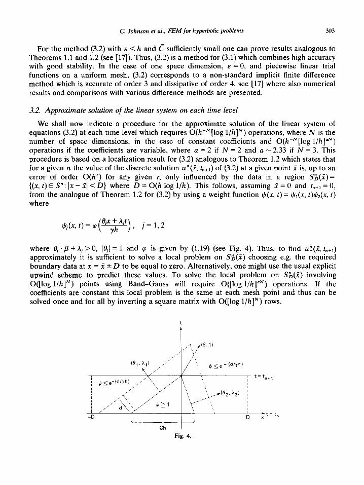
We shall now indicate a procedure for the approximate solution of the linear system of equations (3.2) at each time level which requires O(h+‘[log l/hlN) operations, where N is the number of space dimensions, in the case of constant coefficients and O(heN[log l/hlaN) operations if the coefficients are variable, where a = 2 if N = 2 and a - 2.33 if N = 3. This procedure is based on a localization result for (3.2) analogous to Theorem 1.2 which states that for a given n the value of the discrete solution u!!(R, tn+l) of (3.2) at a given point i is, up to an error of order O(h’) for any given r, only influenced by the data in a region S;(X) = {(x, t)ES”:Ix-.+cD} h w ere D = O(h log l/h). This follows, assuming R = 0 and t,+* = 0, from the analogue of Theorem 1.2 for (3.2) by using a weight function I,@, t) = &(x, t)t,b&, t)
where
where 0j *p + Aj > 0, l0jl = 1 and cp is given by (1.19) ( see Fig. 4). Thus, to find ~“(2, r,+l) approximately it is sufficient to solve a local problem on S&(X) choosing e.g. the required boundary data at x = rl’ k D to be equal to zero. Alternatively, one might use the usual explicit upwind scheme to predict these values. To solve the local problem on S;(X) involving O([log l/hlN) points using Band-Gauss will require O([log l/hlaN) operations. If the coefficients are constant this local problem is the same at each mesh point and thus can be solved once and for all by inverting a square matrix with O([log l/hlN) rows.
t
t
- (dlyh 1 ‘\\ , *Se 5
I t=t
I n+l
, , I
(0,. A*) /
/ I
D ;t=t,
1 I ,
Ch
Fig. 4.
304 C. Johnson et al., FEM for hyperbolic problem
Thus, to sum up, it is possible to solve the linear system of equations (3.2) with O([log l/hjN) and O([log l/h]“N) operations per mesh point in the cases of constant and variable coefficients, respectively, where a = 2 if N = 2 and a - 2.33 if N = 3.
4. Friedrichs’ systems
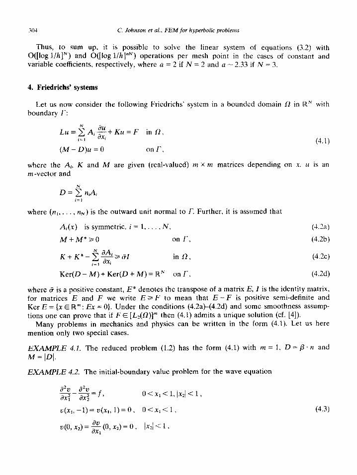
Let us now consider the following Friedrichs’ system in a bounded domain fl in RN with boundary r:
Lu-~Ai~+Ku=F in 0, i=l I
(M-D)u=O on I‘,
where the Ai, K and M are given (real-valued) m X m matrices depending on x, u is an m-vector and
where (nI, . . . , nN) is the outward unit normal to f. Further, it is assumed that
Ai is symmetric, i = 1, . . . , N, (-I.&)
M+M*aO on r, (4.2b)
in fz. (4.2~1
Ker(D - M) + Ker(D + M) = RN on I’, (4.2d)
where E7 is a positive constant, E* denotes the transpose of a matrix E, 1 is the identity matrix, for matrices E and F we write E 2 F to mean that E - F is positive semi-definite and KerE={xER”: Ex = 0). Under the conditions (4.2ab(4.2d) and some smoothness assump- tions one can prove that if FE [L2(,R)Im then (4.1) admits a unique solution (cf. [4]).
Many problems in mechanics and physics can be written in the form (4.1). Let us here mention only two special cases.
EXAMPLE 4.1. The reduced problem (1.2) has the form (4.1) with m = 1, D = p . n and M = ID(.
EXAMPLE 4.2. The initial-boundary value problem for the wave equation
a2v a2v ----T-2- ax, ax2 -A 0 < Xl < 1, Ix*/ < 1 1
I.&,--l)=u(x*,l)=O, o<xl<l, (4.3)
v(O, x2) = z (0, x*) = 0, /x2/ < 1 *
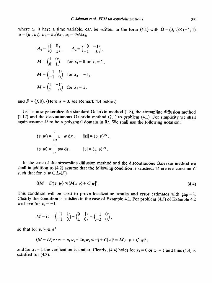
C. Johnson et al., FEM for hyperbolic problems 305
where x1 is here a time variable, can be written in the form (4.1) with 0 = (0,l) x (-1, l), u = (Us, u*), u1 = Allah,, u2 = avlax2,
A2= (_; -;),
M= ( 1 0 0 ) = 1 for x1 0 or x1 = 1 ,
forX2=-1,
for x2 = 1 ,
and F = (f, 0). (Here 6 = 0, see Remark 4.4 below.)
Let us now generalize the standard Galerkin method (1.8) the streamline diffusion method (1.12) and the discontinuous Galerkin method (2.1) to problem (4.1). For simplicity we shall again assume 0 to be a polygonal domain in R2. We shall use the following notation:
(v, w) = j- v - w dx, \\v11= (v, v)“~, R
(v,w)=l vwds, Iv,1 = (v, v)“2. r
In the case of the streamline diffusion method and the discontinuous Galerkin method we shall in addition to (4.2) assume that the following condition is satisfied: There is a constant C such that for v, w E L,(r)
((M - D)v, w) s (Mu, v) + Cl w12. (4.4)
This condition will be used to prove localization results and error estimates with gap = i. Clearly this condition is satisfied in the case of Example 4.1. For problem (4.3) of Example 4.2 we have for x2 = -1
M-D= (-: ;)-(y i)=(_i i)> so that for v, w E R2
and for x2 = 1 the verification is similar. Clearly, (4.4) holds for x1 = 0 or x1 = 1 and thus (4.4) is satisfied for (4.3).
306 C. Johnson et al., FEM for hyperbolic problems
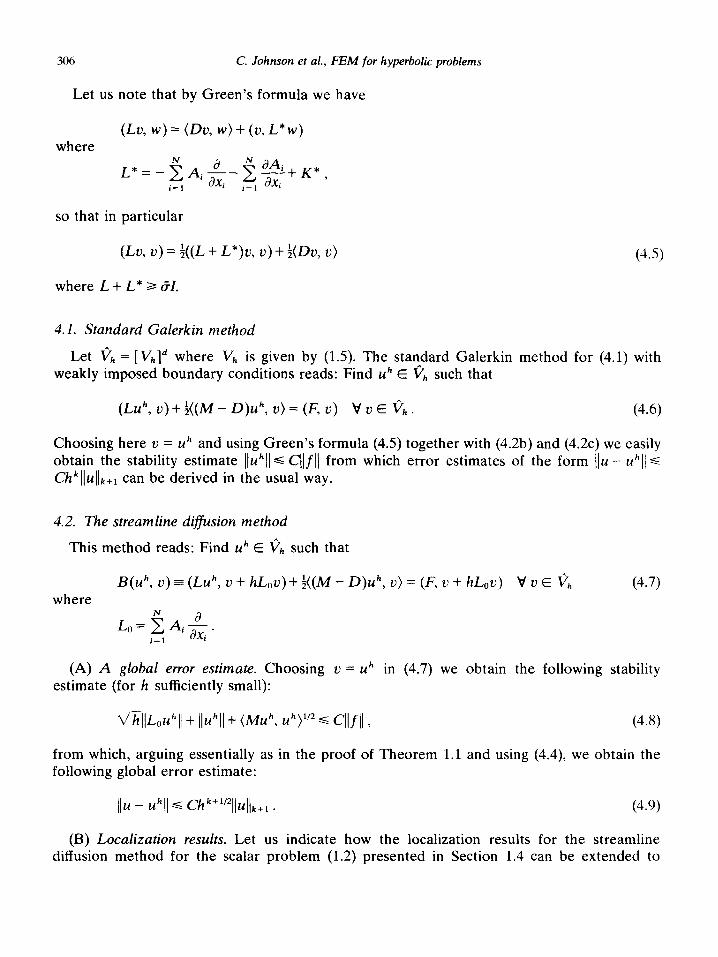
Let us note that by Green’s formula we have
where
so that in particular
(4.5)
where L + L* 3 ~3.
4.1. Standard Galerkin method
Let Qh = [ Vhld where V,, is given by (1.5). The standard Galerkin method for (4.1) with weakly imposed boundary conditions reads: Find uh E ph such that
(LUh, v) + K(M - 0) uh, v) = (F, u) v 2, E v,, . (4.6)
Choosing here I.I = uh and using Green’s formula (4.5) together with (4.2b) and (4.2~) we easily obtain the stability estimate lluhll s ~llfll f rom which error estimates of the form IIu - ~~11 s Chkllullk+I can be derived in the usual way.
4.2. The streamline diffusion method
This method reads: Find uh E +h such that
B(uh, U) = (Luh, u + hL,u)+ $((M - D)uh, v) = (F, 2, + hLou) v ?I E v,, where
(4.7)
L,=2Ai&. i=l I
(A) A global error estimate. Choosing ZI = uh in (4.7) we obtain the following stability estimate (for h sufficiently small):
kqlL,uhI( + llUhll + (Md, UhY2 9 Cllfll 3 (4.8)
from which, arguing essentially as in the proof of Theorem 1.1 and using (4.4), we obtain the following global error estimate:
IIU - Uh(l 6 Chk+“‘I(uI(k+, . (4.9)
(B) Localization results. Let us indicate how the localization results for the streamline diffusion method for the scalar problem (1.2) presented in Section 1.4 can be extended to
C. Johnson et al., FEM for hyperbolic problems 307
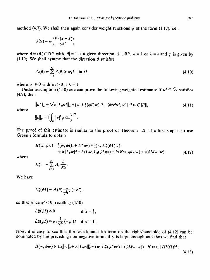
method (4.7). We shall then again consider weight functions + of the form (1.17), i.e.,
where 8 = (8,) E RN with jel= 1 is a given direction, Z E RN, A = 1 or A = $ and cp is given by (1.19). We shall assume that the direction 0 satisfies
A(8) e 5 Ai0i 2 ~11 in L! (4.10) i=l
where aI20 with CT~>O if A = 1. Under assumption (4.10) one can prove the following weighted estimate: If uh E ph satisfies
(4.7) then
where lldy+ + dilpL,dll* +(w, L;($I)w)1’2 + bwe UhY s cll~ll~ (4.11)
lI4Is = (I, b-4*1(1 q* *
The proof of this estimate is similar to the proof of Theorem 1.2. The first step is to use Green’s formula to obtain
B(w, $w) = l(w, (cI(L + L*)w) + l(w, G($I)w) + hllLowll*+ h(Lw, Lo(#I)w) + h(Kw, I,&w)+ %+Mtv, w>
where
Lt=-5Ai&e i=l I
(4.12)
We have
so that since cp’ < 0, recalling (4.10)
L~(t+GI)~O if A = 1,
(-cp’)l if A = 1 .
Now, it is easy to see that the fourth and fifth term on the right-hand side of (4.12) can be dominated by the preceding non-negative terms if y is large enough and thus we find that
B(W, $w) 2 C(llwll:+ hllLowll:+ (w, G($~)w)+ (Ww 4) v w E tff’(Wl”. (4.13)
308 C. Johnson et al., FEM for hyperbolic problems
Proceeding now as in the proof of Theorem 1.2 we obtain the desired weighted estimate (4.11).
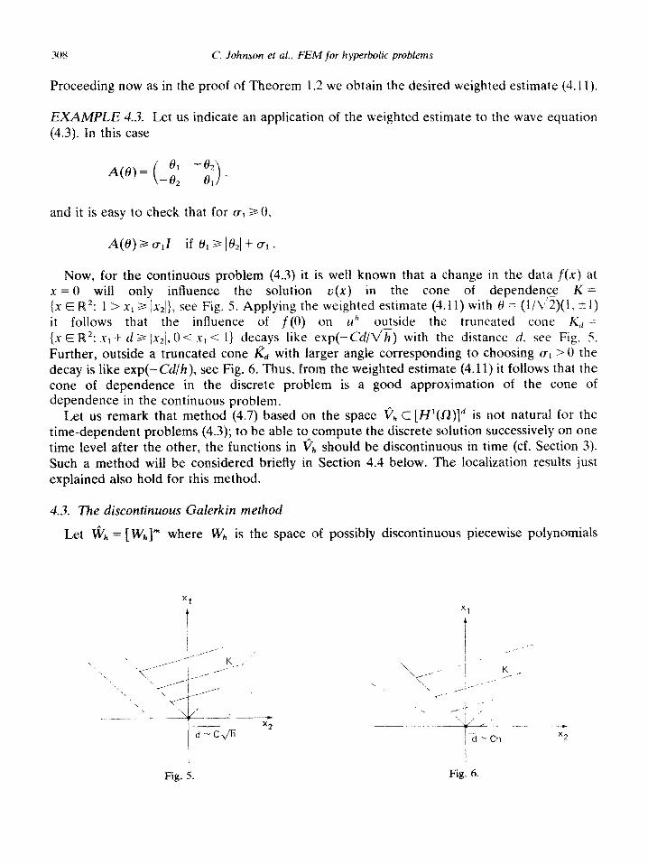
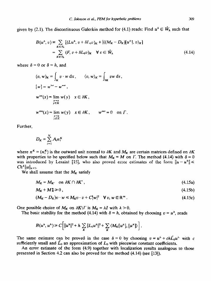
~XA~~~~ 4.3. Let us indicate an application of the weighted estimate to the wave equation (4.3). In this case
and it is easy to check that for o1 2 0,
Now, for the continuous problem (4.3) it is well known that a change in the data f(x) at x = 0 will only influence the solution v(x) in the cone of dependence K = {x E I@: 1 > xr 2 /x2/}, see Fig. 5. Applying the weighted estimate (4.11) with 0 = (l/C’~)(l, + I) it follows that the influence of f(O) on 14” outside the truncated cone K,, =
{x E R2: x1 -t d 2 1x2/, I) < xl < l} decays like exp(-C&/h) with the distance d, see Fig. 5.
Further, outside a truncated cone & with larger angle corresponding to choosing cl > 0 the decay is like exp(- Cd/h), see Fig. 6. Thus, from the weighted estimate (4.11) it follows that the cone of dependence in the discrete problem is a good approximation of the cone of dependence in the continuous problem.
Let us remark that method (4.7) based on the space p,, C [N’(S2)Id is not natural for the time-dependent problems (4.3); to be able to compute the discrete solution successively on one time level after the other, the functions in rib should be discontinuous in time (cf. Section 3). Such a method will be considered briefly in Section 4.4 below. The localization results just explained also hold for this method.
4.3. The discontinuous GaZerkin method
Let VVh = [Wkjrn where ?V, is the space of possibly discontinuous piecewise polynomials
Xl
1
--t x2
Fig, 5. Fig. 6.
C. Johnson et al., FEM for hyperbolic problems 309
given by (2.1). The discontinuous Galerkin method for (4.1) reads: Find uh E I6$ such that
B(Uh, u)= 2 [(L Uh, ZJ + ~JhU)K + mfK - DK)[Uhl, 4Kl KETI,
= 2 (I;,+&u)K \du-&
KETk
(4.14)
where 6 = 0 or 6 = h, and
(~Aw)K=~ ti.wdx, K
{t.~,w)~=j- vwds, dK
Iw] =: Wint - WeXf ,
wint(x) = lim w(y) x E cX, ys
wMt(x) = lim w(y) x E dK, weX’ = 0 on 1”. ,‘z
Further,
where nK = (nf) is the outward unit normal to HC and &I” are certain matrices defined on 6K with properties to be specified below such that I& = M on T. The method (4.14) with S = 0 was introduced by Lesaint [15], who also proved error estimates of the form I/u - u’/ < Chkth&+,.
We shall assume that the MK satisfy
One possible choice of I& on X\r is A& = AI with h > 0. The basic stability for the method (4.14) with 8 = h, obtained by choosing Z.I = u”, reads
B(Uh, Uh)3 +bhtl’+ h c /&uht~+ c <MK[Uh], [u”l)] . K K
The same estimate can be proved in the case 6 = 0 by choosing u = rP + chi&,u” with c su~ciently small and g, an approximation of Lo with piecewise constant coefficients.
An error estimate of the form (4.9) together with localization results analogous to those presented in Section 4.2 can also be proved for the method (4.14) (see [13]).
310 C. Johnson et al., FEM for hyperbolic problems
4.4. Time-dependent problems
Let us now consider a Friedrichs’ system of the form
(4.16a)
on (0, T)x r,
XER,
(4.16b)
(4.16c)
where the Ai, K and A4 are matrices depending on (t, x) satisfying conditions (4.2a)-(4.2d) now on (0, T) X f or (0, T) X 62. In fact (4.16) can be viewed as a special case of (4.1) with A, = I and M = I for x1 = 0 or x1 = T. Thus we can directly apply the discontinuous Galerkin method (4.14) to (4.16) using finite element triangulations of the strips S, = (t,, tn+l) X 0 as in Section 3. With such a method it will be possible to compute the discrete solution on one strip after the other since on the ‘top’ part of X$, where t = tn+l, we have M - D = 0.
Alternatively we may on each strip S,, use a finite element space V; C [H’(S,)]” and seek an approximate solution u” E Vi satisfying
(Lu”, 2) + hLou)” + I uY(t,, x)- u+(t,, x)dx = n
= (F, v + h&u)” + ul(t,, x) . u+(t,, x)dx V u E V; (4.17)
where we use the obvious generalization to the vector case of the notation for the scalar problem (3.2), and
The error estimates and the localization results presented in Section 4.2 can be extended to method (4.17). In particular we have for this method results for the cone of dependence analogous to those discussed in Example 4.3. Roughly speaking these results can be stated as follows in the case the Ai are constant: Suppose uO(x) = 0 if x * 8 > 0 where 8 E RN is given, loI= 1. Suppose that A 2 A,,,&@ where A ,,,(e) denotes the largest eigenvalue of the matrix
A(8) = 5 @Ai. i=l
Then, for the discrete solution uh defined by u,,ls. = u”, we have
IIGL C Cexp(-C&) (4.18)
C. Johnson et al., FEM for hyperbolic problems 311
where 11 * lId,A d enotes the L*-norm over the region
H& = {(f, x): x - 8 2 At + d} n (0, T) x 0.
If A > Amax then the right-hand side of (4.18) can be replaced by C exp(-C&h). Notice that the exact solution vanishes in {(t, x): x . 8 2 A,&0)t}.
The method (4.17) as well as the discontinuous Galerkin method applied to (4.16) lead to systems of equations to be solved on each time strip. Using the localization results for these methods just stated we obtain results on the approximate solution of these systems of equations which are analogous to those presented in Section 3.2.
REMARK 4.4. It is always possible to introduce a positive zero-order term in (4.16a) (corresponding to assuming that 5 > 0 in (4.2~)) by using the change of unknown w(t) = e-%(t) with cr positive. Alternatively one may introduce a corresponding term in the bilinear form by using a weight function $(t) = e-“‘. In both cases the result is an exponential factor eaT in the error estimates which is not satisfactory if T is not moderately small. However, in an incremental scheme for (4.16) the a/at-term can be used to give the desired control of the Lz-norm of the discrete solution and exponential weighting in time with t&(t) = e-“’ can be avoided. Thus, for (4.16) it is sufficient to assume that the constant a in (4.2~) satisfies CJ 2 0 (see [ 171).
References
[l] P. Brenner and V. Thorn&e, Estimates near discontinuities for some difference schemes, Math. Stand. 27
(1970) S-23. [2] A. Brooks, A Petrov-Galerkin finite element formulation for convective dominated flows, Thesis, CALTEC,
1981. [3] P.G. Ciarlet, The finite Element Method for Elliptic Problems (North-Holland, Amsterdam, 1978).
[4] K.O. Friedrichs, Symmetric positive differential equations, CPAM (1958) 333-418. [5] T.J.R. Hughes and A. Brooks, A multidimensional upwind scheme with no crosswind diffusion, in: T.J.R.
Hughes, ed., Finite Element Methods for Convection Dominated Flows, AMD Vol. 34 (ASME, New York,
1979). [6] T.J.R. Hughes and A. Brooks, A theoretical framework for Petrov-Galerkin methods with discontinuous
weighting functions: Application to the Streamline-upwind procedure, to appear in: R.H. Gallagher, ed.,
Finite Elements in Fluids, Vol. 4 (Wiley, New York). [7] T.J.R. Hughes, T.E. Tezduyar and A. Brooks, Streamline upwind formulation for advection-diffusion,
Navier-Stokes and first order hyperbolic equations, Fourth Intemat. Conf. on Finite Element Methods in Fluids, Tokyo, 1982.
[8] P. Jamet, Galerkin-type approximations which are discontinuous in time for parabolic equations in a variable domain, SIAM J. Numer. Anal. 15 (1978) 912-928.
[9] C. Johnson and U. Navert, An analysis of some finite element methods for advectiondiffusion problems, in:
0. Axelsson, L.S. Frank and A. van der Sluis, eds., Analytical and Numerical Approaches to Asymptotic Problems in Analysis (North-Holland, Amsterdam, 1981).
[lo] C. Johnson, Finite element methods for convection+liffusion problems, in: R. Glowinski and J.L. Lions, eds., Computing Methods in Engineering and Applied Sciences V (North-Holland, Amsterdam, 1982).
[ll] C. Johnson and J. Pitkiiranta, Convergence of a fully discrete scheme for two-dimensional neutron transport, SIAM J. Numer. Anal. 20 (1983) 951-966.
313 C. Johnson et al.. FEM for hyperbolic problems
[12] C. Johnson and J. Pitkaranta, An analysis of the discontinuous Galerkin method for a scalar hyperbolic equation, Tech. Rept.. Technical University of Helsinki, 1984.
[ 131 C. Johnson and Huang Mingyou, An analysis of the discontinuous Galerkin method for Friedrichs’ systems, to appear.
[14] P. Lesaint and P.A. Raviart, On a finite element method for solving the neutron transport equation, in: C. de Boor, ed., Mathematical Aspects of Finite Elements in Partial Differential Equations (Academic Press. New York, 1974).
[15] P. Lesaint, Sur la resolution des systemes hyperboliques du premier ordre par de methodes d’elements finis, These, Universite Paris VI, 1975.
[16] J. Nitsche and A. Schatz, Interior estimates for Ritz-Galerkin methods. Math. Comput. 28 (1974) 937-958. [17] U. Navert. A finite element method for convectionaiffusion problems, Thesis, Chalmers Univ. of Technology.
Goteborg, 1982.
[18] G.D. Raithby, Skew upstream differencing schemes for problems involving fluid flow, Comput. Meths. Appl. Mech. Engrg. 9 (1976) 153-164.
[19] V. ThomCe, Some interior estimates for semidiscrete Galerkin approximations for parabolic equations, Math. Comput. 33 (1979) 37-62.
[20] M.I. Vishik and L.A. Lyusternik, Regular degeneration and boundary layer for linear differential equations with a small parameter, Uspekki Mat. Nauk. 12 (1957) 3122: Amer. Math. Sot. Transl. Ser. 2 20 (1962)
239-364.