Finite Element Simulations of MicrobeamBending ExperimentsMaster’s thesis in Applied Mechanics

JOHN WIKSTROM

Department of Applied MechanicsCHALMERS UNIVERSITY OF TECHNOLOGYGoteborg, Sweden 2017

MASTER’S THESIS IN APPLIED MECHANICS

Finite Element Simulations of Microbeam Bending Experiments

JOHN WIKSTROM

Department of Applied MechanicsDivision of Material & Computational MechanicsCHALMERS UNIVERSITY OF TECHNOLOGY

Goteborg, Sweden 2017

Finite Element Simulations of Microbeam Bending Experiments

JOHN WIKSTROM

c© JOHN WIKSTROM, 2017

Master’s thesis 2017:42ISSN 1652-8557Department of Applied MechanicsDivision of Material & Computational MechanicsChalmers University of TechnologySE-412 96 GoteborgSwedenTelephone: +46 (0)31-772 1000

Cover: Displacement plot from a microbeam bending simulation.

Chalmers ReproserviceGoteborg, Sweden 2017

Finite Element Simulations of Microbeam Bending Experiments

Master’s thesis in Applied MechanicsJOHN WIKSTROMDepartment of Applied MechanicsDivision of Material & Computational MechanicsChalmers University of Technology

Abstract

The microstructure of metals is built up by grains. Each grain in turn has an anisotropic crystal structure withan individual crystal orientation. The mechanical behavior of single crystals can be modeled using so calledcrystal plasticity models. These crystal plasticity models are typically used as constitutive models in finiteelement analyses.

Multiscale modeling strategies may be used to link the micromechanical crystal behavior to the behavior ofmetals on the macroscale. In practice, it is the macroscale response that is of importance when assessing theperformance of engineering components in the industry. However, for a multiscale analysis to be successful, werequire an accurate crystal plasticity model for the metal of interest. It is today possible to perform experimentson the microscale with structures made from single crystals. Data from these experiments may then be used tocalibrate a crystal plasticity model. Calibration here refers to the process of fitting a simulation response tothe experimental data by finding the best values for the material parameters in the constitutive model.

The main objective of this thesis is to investigate the possibilities to use data from microbeam bendingexperiments in order to calibrate a specific crystal plasticity model. The microbeam bending experimentscan be described as cantilever beam experiments in which each of the beams are subjected to a displacementcontrolled point load. During the experiments, photos are taken in order to evaluate force-deflection data forthe contact point. The experiments were prepared and conducted by Anand Harihara Subramonia Iyer at theDepartment of Physics at Chalmers. Three microbeams were prepared in total for the experiments. Each ofthe microbeams was milled out from a single crystal of the superalloy Allvac 718 Plus. The three microbeamshad different geometry and crystal orientation. One of the experiments was successful while the other twoexperiments unfortunately failed.

The first step in the project was to develop a finite element model in Abaqus which can be used to simulatemicrobeam bending experiments. An Abaqus Python script was written to set up the microbeam model. Thisscript was written in a parametrized manner such that the user can specify the individual beam geometry,material parameters and important analysis settings. In order to use the specific crystal plasticity model asconstitutive model in the Abaqus simulations, the microbeam model features a user-defined material model(UMAT). The UMAT was implemented by Magnus Ekh at the Department of Industrial and Materials Scienceat Chalmers.

The next step was to set up an optimization routine which can be used to calibrate the material parametersof the crystal plasticity model based on experimental data. This was achieved by coupling optimization code inMatlab with Abaqus simulations. The Nelder-Mead method, also called the simplex method, was chosen asoptimization algorithm for this purpose.

Since limited data was acquired in the experiments, a calibration was first performed based on “experimentdata” produced by three different microbeam finite element models. These microbeam models all had the samegeometry but different crystal orientation. The data was produced with a known set of material parametervalues which were then disturbed and “calibrated”. In the case of a well-formulated optimization problem,the material parameter values used to produce the data are hopefully found in the calibration. The problemof calibrating the elastic parameters resulted in a non-unique solution. It was concluded that more responseinformation is needed from the experiments (and the simulations) in order to uniquely find all the elasticparameters, force-deflection data is not enough. Calibration of the plastic responses were performed taking alimited set of the plastic material parameters into consideration. This decision was taken in order to promote aunique solution. It was judged that calibration of the omitted parameters would require more advanced responsedata, e.g. data for different load rates. Overall, the fictitious calibration resulted in well fitted force-deflectionresponse curves. It was also concluded that the sensitivity for some plastic material parameters were higherthan for other ones.

A calibration based on data from the real microbeam bending experiment was then performed. It waspossible to obtain a well fitted force-deflection response through a calibration process. However, due to the

non-unique solution for the elastic parameters, two constraints that can be considered arbitrary were used. Also,the experimental data showed an overly stiff linear elastic response compared to the finite element simulationwhen using material parameters for the similar superalloy Inconel 718. This is probably due to inaccurateexperimental data. In conclusion, the calibrated material parameters for Allvac 718 Plus resulted in a goodresponse fit but is unlikely representative for the material.

In relation to the calibration, comparisons between the slip lines obtained in the experiments and the slipvariables in the simulations were performed. These comparisons involved images from all experiments, includingthe ones that failed. However, no major conclusions could be made from these comparisons.

Keywords: crystal plasticity, microbeam bending, material model calibration

ii

Preface

First of all I would like to thank my supervisor and examiner Magnus Ekh for his great support and helpthroughout the project. His invaluable knowledge and experience in constitutive modeling kept me on trackand saved me trouble at several stages the last five months. I would also like to thank Magnus Colliander andAnand Harihara Subramonia Iyer for giving me an insight into their world of microscale experiments withmetals. I hope that my thesis work in some way can contribute to your future research on crystal plasticity.

John WikstromGoteborg, June 2017

iii

iv

Contents

Abstract i

Preface iii

Contents v

1 Introduction 11.1 Background & Motivation . . . . . . . . . . . . . . . . . . . . . . . . . . . . . . . . . . . . . . . . . 11.2 Thesis Objectives . . . . . . . . . . . . . . . . . . . . . . . . . . . . . . . . . . . . . . . . . . . . . . 11.3 Report Structure . . . . . . . . . . . . . . . . . . . . . . . . . . . . . . . . . . . . . . . . . . . . . . 2

2 Microbeam Bending 3

3 Crystal Plasticity 63.1 Notations . . . . . . . . . . . . . . . . . . . . . . . . . . . . . . . . . . . . . . . . . . . . . . . . . . 63.2 Crystal Orientations . . . . . . . . . . . . . . . . . . . . . . . . . . . . . . . . . . . . . . . . . . . . 63.2.1 Euler Angles (Bunge Convention) . . . . . . . . . . . . . . . . . . . . . . . . . . . . . . . . . . . 63.2.2 Rotation Matrix . . . . . . . . . . . . . . . . . . . . . . . . . . . . . . . . . . . . . . . . . . . . . 83.2.3 Tensor Transformations . . . . . . . . . . . . . . . . . . . . . . . . . . . . . . . . . . . . . . . . . 83.3 Elastic Cubic Symmetry . . . . . . . . . . . . . . . . . . . . . . . . . . . . . . . . . . . . . . . . . . 93.3.1 Apparent Young’s Modulus . . . . . . . . . . . . . . . . . . . . . . . . . . . . . . . . . . . . . . . 93.4 Crystal Plasticity . . . . . . . . . . . . . . . . . . . . . . . . . . . . . . . . . . . . . . . . . . . . . . 93.4.1 Slip Systems . . . . . . . . . . . . . . . . . . . . . . . . . . . . . . . . . . . . . . . . . . . . . . . 93.4.2 Governing Equations . . . . . . . . . . . . . . . . . . . . . . . . . . . . . . . . . . . . . . . . . . . 113.4.3 Yield Surface Interpretation . . . . . . . . . . . . . . . . . . . . . . . . . . . . . . . . . . . . . . . 123.5 Implementation . . . . . . . . . . . . . . . . . . . . . . . . . . . . . . . . . . . . . . . . . . . . . . . 123.5.1 Local Constitutive Problem . . . . . . . . . . . . . . . . . . . . . . . . . . . . . . . . . . . . . . . 143.5.2 Global Structural Problem . . . . . . . . . . . . . . . . . . . . . . . . . . . . . . . . . . . . . . . 15

4 Microbeam Finite Element Model 164.1 Parametrized Microbeam Model . . . . . . . . . . . . . . . . . . . . . . . . . . . . . . . . . . . . . 164.2 Element and Convergence Analysis . . . . . . . . . . . . . . . . . . . . . . . . . . . . . . . . . . . . 174.3 Example Simulations . . . . . . . . . . . . . . . . . . . . . . . . . . . . . . . . . . . . . . . . . . . . 18

5 Calibration of Crystal Plasticity Model 215.1 Mathematical Formulation . . . . . . . . . . . . . . . . . . . . . . . . . . . . . . . . . . . . . . . . . 215.2 Calibration Based on Fictitious Data . . . . . . . . . . . . . . . . . . . . . . . . . . . . . . . . . . . 225.2.1 Finding Elastic Parameters C11, C12 and C44 . . . . . . . . . . . . . . . . . . . . . . . . . . . . . 245.2.2 Finding Plastic Parameters h∞, h0, τ∞ and τ0 . . . . . . . . . . . . . . . . . . . . . . . . . . . . 245.2.3 Parameters qαα and qαβ . . . . . . . . . . . . . . . . . . . . . . . . . . . . . . . . . . . . . . . . . 255.3 Calibration Based on Experimental Data . . . . . . . . . . . . . . . . . . . . . . . . . . . . . . . . 305.3.1 Finding Elastic Parameters C11, C12 and C44 . . . . . . . . . . . . . . . . . . . . . . . . . . . . . 305.3.2 Finding Plastic Parameters h∞, h0, τ∞ and τ0 . . . . . . . . . . . . . . . . . . . . . . . . . . . . 305.3.3 Slip Systems Verification . . . . . . . . . . . . . . . . . . . . . . . . . . . . . . . . . . . . . . . . 325.4 Boundary Conditions Study . . . . . . . . . . . . . . . . . . . . . . . . . . . . . . . . . . . . . . . . 38

6 Concluding Remarks 406.1 Suggestions for Future Work . . . . . . . . . . . . . . . . . . . . . . . . . . . . . . . . . . . . . . . 41

References 43

A Abaqus Python Scripting IA.1 Model Setup Script . . . . . . . . . . . . . . . . . . . . . . . . . . . . . . . . . . . . . . . . . . . . . IA.2 Postprocessing Script . . . . . . . . . . . . . . . . . . . . . . . . . . . . . . . . . . . . . . . . . . . I

v

B Calibration Programming II

vi

1 Introduction1.1 Background & MotivationSuperalloys is a class of alloys where its members show excellent mechanical properties in multiple regards.The combination of high mechanical strength at high temperatures accompanied with excellent corrosionand oxidation resistance makes superalloys suitable for some of the most extreme engineering applications.Within the group of superalloys, the nickel-based ones tend to stand out with extraordinary good properties.Nickel-based superalloys have gained extra traction within the aerospace and aircraft industry where they arecommonly used in gas turbine engines. However, the properties of nickel-based superalloys are utilized in otherapplications as well, e.g. marine ships, nuclear reactors and defense industry applications [1].

The macroscale mechanical properties of a metal are strongly dependent on its microstructural compositionwhich in turn depends on the constituents and the manufacturing process. Regarding modeling of the microscaleof metals, various crystal plasticity models have been developed over the years and implemented as constitutivemodels in finite element analyses. If an accurate material model is available for the microscale, it can be usedin a multiscale modeling strategy to numerically link the macroscale properties to those of the microscale, seeFigure 1.1. Experiments on the microscale could thereby play a key role in any multiscale modeling strategy.In particular, data from such experiments can be used to calibrate crystal plasticity models.

In order to gain further knowledge of the microscale mechanical behavior of superalloys, microbeam bendingexperiments have recently been initiated at the Department of Physics, Chalmers. These experiments featuremicrobeams with lengths of 10 to 20 µm which each are milled from a single crystal. The studied material inthese experiments is the nickel-based superalloy Allvac 718 Plus which is of special interest for the aerospaceindustry. In this thesis, the possibility to calibrate a crystal plasticity model based on data from microbeambending experiments is investigated.

1.2 Thesis ObjectivesThe main purposes of this thesis are related to assisting in the establishment of a computational modelingplatform for crystal plasticity at Chalmers. More specifically, a finite element model should be developed forAbaqus such that microbeam bending experiments can be simulated. An already implemented crystal plasticityuser-defined material model (UMAT) is available as a user subroutine for Abaqus.

The finite element model should be generated from an Abaqus Python script to ensure a correct andconsistent model setup. The model build-up from the script should be highly parametrized such that theuser is able to specify microbeam dimensions, crystal orientation, material properties, mesh properties and

Crystal plasticity

Engineeringcomponent

Figure 1.1: Illustration of multiscale modeling of metals.

1

some important analysis settings. It should also be possible to include an oxide layer on top of the microbeamstructure.

Besides finite element model development, another objective is to develop a procedure in which microbeamsimulations in Abaqus can be coupled with external optimization code. The optimization code should be ableto make changes in material parameters and call new simulation jobs. The corresponding model response forgiven material parameters is then compared to experimental data as the definition of an objective function.The final task is to calibrate the crystal plasticity model based on the data from the microbeam bendingexperiments for the Allvac 718 Plus superalloy.

1.3 Report StructureIn Chapter 2, a description of the microbeam bending experiments is presented. This chapter covers the processof making microbeams, experiment setup and the experiment results. A presentation of crystal plasticity andthe particular constitutive model used in the finite element modeling is given in Chapter 3. In Chapter 4,details about the finite element modeling of the experiments are presented. Chapter 5 treats calibration ofthe crystal plasticity model using the experimental data. The main report ends with Chapter 6 which mostlydiscusses the calibration results and suggestions for future work.

There are also two appendices. The first appendix contains some notes on Python scripting in Abaqus andexplains the scripts used in the project. The second appendix treats the programming for the constitutivemodel calibration. It is in detailed covered how an external program, for example and in this case Matlab, mayperform an engineering optimization task with underlying Abaqus simulations.

2

2 Microbeam BendingThe microbeam bending technique has been used by several authors, e.g. [2] and [3], to study the micromechanicalproperties of materials. This chapter covers the microbeam bending experiments including preparation andresults. The work described here has been performed at the Department of Physics by Anand HariharaSubramonia Iyer. In total, three microbeams were made for the experiments. Each one of the microbeams ismade out of a single crystal of the superalloy material Allvac 718 Plus. The three microbeams have differentcrystallographic orientation relative to a specified beam coordinate system. The crystal orientation for amicrobeam affects its stiffness and the nature of its crystal slip. These effects of the crystal orientation areelaborated further on in Chapter 3.

The microbeams are shaped from a milling process using a FIB (focused ion beam) technique. Material isremoved until the shape is satisfying and the beam structure looks like in the illustration in Figure 2.1. Sincethe milling process is a difficult one, the microbeam geometry measures will have some uncertainties. Thegeometry and orientation for each one of the three microbeams are given in Table 2.1 where the dimensionsrefer to Figure 2.1. The crystal orientations are presented in Euler angles using the Bunge convention. Theseangles are explained in detail in Section 3.2. The crystal orientations are measured with a technique calledEBSD which is short for electron backscatter diffraction.

The experiment setup is illustrated in Figure 2.1. To prevent oxidation of the metal, the experiment isconducted in a vacuum environment. The whole specimen containing the grain of interest is attached to aspring table with a known stiffness (spring constant). The beam is then deflected by applying a point load witha diamond tip tool close to the tip of the beam. During the experiment, SEM (scanning electron microscope)images are recorded. The displacement of the whole specimen is measured from these images by tracking a firstreference point, denoted A in Figure 2.1. The force applied in the diamond tip contact can then be evaluatedfrom force equilibrium since the spring stiffness is known. In order for this concept to work, point A mustbelong to a non-deforming (or negligibly deforming) part of the specimen. The contact point B is tracked aswell. By evaluating the displacement of point B relative to A, the beam deflection can be computed.

The experiment with microbeam B was successfully conducted. A force-deflection data plot for thisexperiment is given in Figure 2.2. Unfortunately, the experiments with microbeams A and C failed. Fordifferent reasons, these microbeams were not deformed in the way that was planned and no useful data wasobtained. Images of the microbeams after the experiments are presented in Figure 2.3. Microbeams A and C(failed experiments) show signs of notable torsional deformation.

Table 2.1: Geometries and crystal orientations for the microbeams used in the experiments.

Experiment beams

Beam Geometry Orientation

L (µm) w (µm) h (µm) r (µm) ϕ1 Φ ϕ2

A 10.45 4.2 3.6 0.4 302.3◦ 40.7◦ 56.1◦

B 13.0 3.0 3.9 0.11 79.3◦ 6.8◦ 36.9◦

C 11.8 4.0 3.8 0.35 247.4◦ 41.9◦ 68.1◦

3

diamond tip

microbeam

A

spring

B

x

z

o

y

B

yz-view of themicrobeam

(vacuum)

L

r

h

w

Figure 2.1: Illustration of the microbeam bending experiment setup and the microbeam dimensions.

0

500

1000

1500

2000

0 1 2 3 4 5 6

Force(µN)

Deflection (µm)

Experiment B

Figure 2.2: Force-deflection data from the successful experiment with microbeam B. Images for data evaluationwas acquired once per second. The total time elapsed up to the point of unloading is approximately 100 seconds.

4

Microbeam A

Microbeam B

Microbeam C

Figure 2.3: SEM images from an xz-view of microbeams A, B and C after the experiments.

5

3 Crystal PlasticityA thorough overview of the basics of crystal plasticity modeling is given in e.g. Reference [4]. Here, only themain modeling features are presented. For clarity of presentation, the crystal plasticity model formulation is hererestricted to small strains. However, the simulation results in this report are produced using a correspondingformulation based on the finite strain theory (large strains).

3.1 NotationsFirst-order tensors or vectors will be denoted by bold-faced and upright italic characters, e.g. a or b. Somebold-faced greek characters represent second-order tensors, like the Cauchy stress tensor σ and the strain tensorε. Bold-faced and calligraphic capital characters will represent tensors of order four. Examples of fourth-ordertensors are the elastic stiffness modulus tensor C and the related compliance tensor C−1. Whenever componentsof tensors are used in expressions, e.g. σij , these refer to a Cartesian coordinate system.

Regarding tensor operations, ⊗ will be used to denote the open product. Scalar product or single contractionis denoted by a single dot ·, whereas : is used for double contraction. An example of double contraction is givenby

C : ε = Cijklεkl ei ⊗ ej . (3.1)

3.2 Crystal OrientationsSince single crystals in general are anisotropic, it is important to properly describe their orientations. Thisis commonly achieved by using Euler angles with the Bunge convention. Throughout this report, the globalreference coordinate system is denoted by oxyz whereas the crystal material coordinate system is given byox′y′z′. The corresponding unit basis vectors are denoted {ei}3i=1 = {e1, e2, e3} and {e′i}

3i=1 = {e′1, e′2, e′3},

respectively.

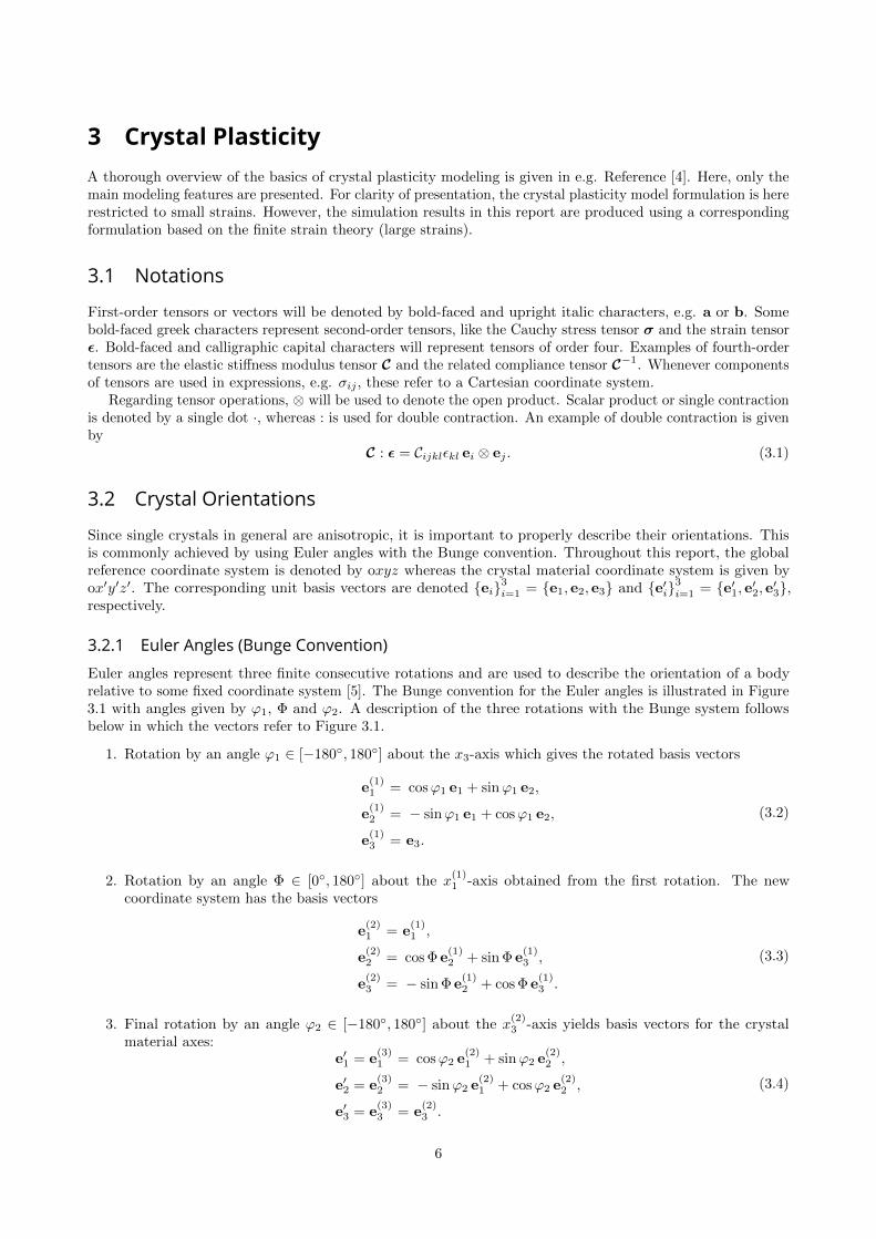
3.2.1 Euler Angles (Bunge Convention)Euler angles represent three finite consecutive rotations and are used to describe the orientation of a bodyrelative to some fixed coordinate system [5]. The Bunge convention for the Euler angles is illustrated in Figure3.1 with angles given by ϕ1, Φ and ϕ2. A description of the three rotations with the Bunge system followsbelow in which the vectors refer to Figure 3.1.

1. Rotation by an angle ϕ1 ∈ [−180◦, 180◦] about the x3-axis which gives the rotated basis vectors

e(1)1 = cosϕ1 e1 + sinϕ1 e2,

e(1)2 = − sinϕ1 e1 + cosϕ1 e2,

e(1)3 = e3.

(3.2)

2. Rotation by an angle Φ ∈ [0◦, 180◦] about the x(1)1 -axis obtained from the first rotation. The new

coordinate system has the basis vectors

e(2)1 = e

(1)1 ,

e(2)2 = cos Φ e

(1)2 + sin Φ e

(1)3 ,

e(2)3 = − sin Φ e

(1)2 + cos Φ e

(1)3 .

(3.3)

3. Final rotation by an angle ϕ2 ∈ [−180◦, 180◦] about the x(2)3 -axis yields basis vectors for the crystal

material axes:e′1 = e

(3)1 = cosϕ2 e

(2)1 + sinϕ2 e

(2)2 ,

e′2 = e(3)2 = − sinϕ2 e

(2)1 + cosϕ2 e

(2)2 ,

e′3 = e(3)3 = e

(2)3 .

(3.4)

6

ϕ1

Φ

ϕ2

e1

e2

e3

e(1)1

e(1)2

e(1)3

e(2)1

e(2)2

e(2)3

e(3)1

e(3)2

e(3)3

(b) First rotation

(c) Second rotation (d) Third rotation

(a) Initial orientation

Figure 3.1: Illustration of the cubic crystal orientation using Euler angles with the Bunge convention.

7

In summary, the transformation of the basis vectors from oxyz to ox′y′z′ using the Bunge convention may bedescribed by the matrix formulation[

e′1 e′2 e′3]

=[e1 e2 e3

]Rϕ1RΦ Rϕ2 (3.5)

where

Rϕ1=

cosϕ1 − sinϕ1 0sinϕ1 cosϕ1 0

0 0 1

, RΦ =

1 0 00 cos Φ − sin Φ0 sin Φ cos Φ

, Rϕ2=

cosϕ2 − sinϕ2 0sinϕ2 cosϕ2 0

0 0 1

. (3.6)

3.2.2 Rotation MatrixA rotation matrix, commonly denoted Q, may be used to transform coordinates from one coordinate system toa rotated coordinate system. The components of Q are defined as projections of the basis vectors between thetwo coordinate systems. For transformations between the two coordinate systems oxyz and ox′y′z′, we maydefine the components of Q as

Qij = e′i · ej . (3.7)

Using Euler angles with the Bunge convention, the transposed rotation matrix is obtained as

QT =

eT1

eT2

eT3

[e′1 e′2 e′3]

=

eT1

eT2

eT3

[e1 e2 e3

]Rϕ1

RΦ Rϕ2= Rϕ1

RΦ Rϕ2(3.8)

where the orthonormality of the vectors {ei}3i=1 was used in the last equality. Equation (3.8) implies that

Q = (Rϕ1RΦ Rϕ2

)T

= RTϕ2

RTΦ RT

ϕ1. (3.9)

Carrying out the matrix multiplication using the matrices in (3.6), we finally end up with

Q =

cosϕ1 cosϕ2 − sinϕ1 cos Φ sinϕ2 sinϕ1 cosϕ2 + cosϕ1 cos Φ sinϕ2 sin Φ sinϕ2

− cosϕ1 sinϕ2 − sinϕ1 cos Φ cosϕ2 − sinϕ1 sinϕ2 + cosϕ1 cos Φ cosϕ2 sin Φ cosϕ2

sinϕ1 sin Φ − cosϕ1 sin Φ cos Φ

. (3.10)

3.2.3 Tensor TransformationsWorking with arbitrary crystallographic orientation, it is necessary to be able to carry out transformations oftensors. Consider the two coordinate systems oxyz and ox′y′z′ (both orthonormal) for which the corresponding

basis vectors are given by {ei}3i=1 and {e′i}3i=1, respectively. A first-order tensor a may be represented in these

two coordinate systems accordingly:a = ai ei = a′j e′j . (3.11)

The component a′i is given by projecting a onto e′i, i.e.

a′i = a · e′i = (aj ej) · e′i = QTjiaj = Qijaj (3.12)

where the components of the rotation matrix Q were used in the last two equalities, here interpreted as atensor. The reverse projection may be set up in the same way:

ai = a · ei = (a′j e′j) · ei = Qjia′j = QT

ija′j . (3.13)

Transformations of higher order tensors follow the same pattern. For instance, the transformations of thefourth-order stiffness tensor C = Cijkl ei ⊗ ej ⊗ ek ⊗ el = C ′mnop e′m ⊗ e′n ⊗ e′o ⊗ e′p are given by

C ′ijkl = QimQjnQkoQlpCmnop (3.14)

andCijkl = QT

imQTjnQ

TkoQ

TlpC′mnop . (3.15)

8

3.3 Elastic Cubic SymmetryLinear elastic cubic symmetry is an appropriate assumption for the elastic behavior of a cubic crystal, c.f.[6]. Apart from the crystal orientation, three elastic material constants are needed in order to describe thestress-strain relationship σ = C : ε in elastic cubic symmetry. These three parameters are commonly denotedC11, C12 and C44. The stiffness tensor for elastic cubic symmetry may be expressed in Voigt form as

[C′]

=

C11 C12 C12 0 0 0 0 0 0C12 C11 C12 0 0 0 0 0 0C12 C12 C11 0 0 0 0 0 00 0 0 2C44 0 0 0 0 00 0 0 0 2C44 0 0 0 00 0 0 0 0 2C44 0 0 00 0 0 0 0 0 2C44 0 00 0 0 0 0 0 0 2C44 00 0 0 0 0 0 0 0 2C44

. (3.16)

The prime superscript ′ on C in (3.16) is used to stress the fact the components refer to the material coordinatesox′y′z′.

3.3.1 Apparent Young’s ModulusThe concept of apparent Young’s modulus can be used to illustrate elastic cubic symmetry. Now, let n be anarbitrary unit vector. The apparent Young’s modulus En relates the normal stress and normal strain in thedirection n for the case of uniaxial stress condition along n. This relation is given by

σn = Enεn (3.17)

whereσn = σ : (n⊗ n) , εn = ε : (n⊗ n) . (3.18)

By substituting (3.18) in (3.17) and using ε = C−1 : σ = σ : C−1, we obtain

σ : (n⊗ n) = En ε : (n⊗ n) = En σ : C−1 : (n⊗ n) (3.19)

which implies that(n⊗ n) = En C−1 : (n⊗ n) . (3.20)

Performing a double dot contraction by n⊗n from the left on both sides, we find the apparent Young’s modulusEn from the equation

1

En= (n⊗ n) : C−1 : (n⊗ n) . (3.21)

As adopted from [7], varying the two first Bunge angles ϕ1 and Φ, we obtain the apparent Young’s modulusplotted in Figure 3.2 along the beam axis. To produce this plot, the following representation of the vector nwas substituted in Equation (3.21):

n =

cosφ sin θsinφ sin θ

cos θ

(3.22)

where angles φ and θ refer to the polar coordinates used in Figure 3.2. For the elastic material parameters wehave here used C11 = 259.6 GPa, C12 = 179.0 GPa and C44 = 109.6 GPa.

3.4 Crystal Plasticity3.4.1 Slip SystemsThe plastic deformation of the crystal lattice, called slip, is more prone to occur in certain planes and directionsdue to the packing of atoms. The slip corresponds to movement of dislocations that is activated by high shear

9

100

150

200

250

300

GPa

x′1x′2

x′3

45◦30◦15◦ 60◦75◦

45◦

60◦

75◦

30◦

15◦

φ

θ

Figure 3.2: The concept of apparent Young’s modulus for a crystal illustrated in spherical coordinates. Maximumis obtained for direction with Miller index [1 1 1] which corresponds to φ = 45.00◦ and θ = 54.74◦.

stress levels. The easiest movement of dislocations, i.e. movement activated by relatively low shear stress levels,occur in the planes and directions with the highest density of atoms. These slip directions and planes are oftenreferred to as “close-packed” directions and planes.

The slip mechanism is modeled using a set of slip systems. Each slip system α is described by a slipdirection sα and a corresponding slip plane described by its normal mα. In total, a set of Nslip slip systems

{(sα,mα)}Nslip

α=1 are considered for the crystal. The superalloys of interest in this thesis, Allvac 718 Plus andthe similar Inconel 718, both have a face centered cubic (FCC) crystal structure [1]. For an FCC crystal, seeFigure 3.3a, the slip planes have members in the Miller index family {1 1 1} and the slip directions belong tothe family 〈1 1 0〉. The slip system family for an FCC crystal is illustrated in Figure 3.3b. All 12 slip systemsfor an FCC crystal are presented in Table 3.1. If slip for a body centered cubic (BCC) crystal is to be modeledinstead, these would need to be substituted.

Table 3.1: The planes and directions of the 12 slip systems for an FCC crystal given in both Miller indices andvector format (local crystal coordinates).

Slip system α Plane Direction

Miller index Normal vector mα Miller index Vector sα

1 (1 1 1) (1, 1, 1) /√

3 [1 1 0] (−1, 1, 0) /√

2

2 (1 1 1) (1, 1, 1) /√

3 [0 1 1] (0,−1, 1) /√

2

3 (1 1 1) (1, 1, 1) /√

3 [1 0 1] (1, 0,−1) /√

2

4 (1 1 1) (−1, 1, 1) /√

3 [1 1 0] (−1,−1, 0) /√

2

5 (1 1 1) (−1, 1, 1) /√

3 [1 0 1] (1, 0, 1) /√

2

6 (1 1 1) (−1, 1, 1) /√

3 [0 1 1] (0, 1,−1) /√

2

7 (1 1 1) (1,−1, 1) /√

3 [1 1 0] (1, 1, 0) /√

2

8 (1 1 1) (1,−1, 1) /√

3 [1 0 1] (−1, 0, 1) /√

2

9 (1 1 1) (1,−1, 1) /√

3 [0 1 1] (0,−1,−1) /√

2

10 (1 1 1) (1, 1,−1) /√

3 [1 1 0] (1,−1, 0) /√

2

11 (1 1 1) (1, 1,−1) /√

3 [1 0 1] (−1, 0,−1) /√

2

12 (1 1 1) (1, 1,−1) /√

3 [0 1 1] (0, 1, 1) /√

2

10

x′3

x′1

x′2

(1 1 1)

[1 0 1] [0 1 1]

[1 1 0]

x′3

x′1

x′2

(a)

(b)

Figure 3.3: (a) Illustration of the atom structure in an FCC crystal. (b) Unit cell illustration of the three slipsystems associated with the plane (1 1 1) for an FCC crystal.

3.4.2 Governing EquationsThe crystal plasticity model used for the simulations in this thesis is adopted from Reference [8]. This materialmodel is based on the finite strain theory. For clarity, the formulation is here presented in a correspondingsmall strain formulation.

The traction vector tα on the slip plane associated with slip system α is obtained by projection of the stresstensor σ onto the corresponding slip plane normal mα, i.e.

tα = σ ·mα. (3.23)

The projected or resolved shear stress in the slip direction, also known as the Schmid stress, is denoted τα andis given by

τα = tα · sα = σ : (mα ⊗ sα) . (3.24)

11

The evolution of the plastic strain εp is assumed to follow the law

εp =

Nslip∑α=1

γα (mα ⊗ sα)sym τα|τα|

(3.25)

where

γα = γ0

(|τα|τ cα

)1/m

sign(τα) α = 1, 2, . . . , Nslip. (3.26)

The variable τ cα is called the critical resolved shear stress associated with slip system α. The evolution of τ c

α isgiven by

τ cα =

Nslip∑β=1

qαβ h(γ) |γβ | α = 1, 2, . . . , Nslip. (3.27)

In Equation (3.27), the Voce hardening model h(γ) was introduced and is given by

h(γ) = h∞ +

[h0 − h∞ +

h0h∞γ

τ∞ − τ0

]exp

(− h0γ

τ∞ − τ0

)(3.28)

where γ refers to the accumulated slip among all slip systems, i.e.

γ(t) =

∫ t

0

Nslip∑α=1

|γα|dt . (3.29)

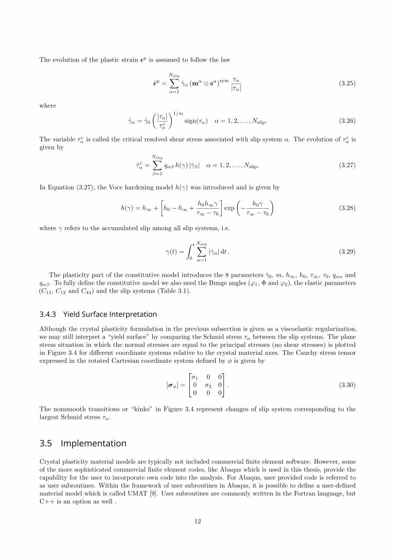
The plasticity part of the constitutive model introduces the 8 parameters γ0, m, h∞, h0, τ∞, τ0, qαα andqαβ . To fully define the constitutive model we also need the Bunge angles (ϕ1, Φ and ϕ2), the elastic parameters(C11, C12 and C44) and the slip systems (Table 3.1).

3.4.3 Yield Surface InterpretationAlthough the crystal plasticity formulation in the previous subsection is given as a viscoelastic regularization,we may still interpret a “yield surface” by comparing the Schmid stress τα between the slip systems. The planestress situation in which the normal stresses are equal to the principal stresses (no shear stresses) is plottedin Figure 3.4 for different coordinate systems relative to the crystal material axes. The Cauchy stress tensorexpressed in the rotated Cartesian coordinate system defined by φ is given by

[σφ] =

σ1 0 00 σ2 00 0 0

. (3.30)

The nonsmooth transitions or “kinks” in Figure 3.4 represent changes of slip system corresponding to thelargest Schmid stress τα.

3.5 ImplementationCrystal plasticity material models are typically not included commercial finite element software. However, someof the more sophisticated commercial finite element codes, like Abaqus which is used in this thesis, provide thecapability for the user to incorporate own code into the analysis. For Abaqus, user provided code is referred toas user subroutines. Within the framework of user subroutines in Abaqus, it is possible to define a user-definedmaterial model which is called UMAT [9]. User subroutines are commonly written in the Fortran language, butC++ is an option as well .

12

x′1x′2

x′3

φ

φ

σ1

σ2

−3

−2

−1

0

1

2

3

−3 −2 −1 0 1 2 3−3

−2

−1

0

1

2

3

−3 −2 −1 0 1 2 3

σ2/τ 0

σ1/τ0

φ = 0◦ φ = 15◦

σ2/τ 0

σ1/τ0

φ = 30◦ φ = 45◦

Figure 3.4: Plane stress yield surface interpretations for a principal stress condition obtained for the crystalplasticity model. The principal stress axes are defined by the angle φ relative the crystal material axes. Planestress is given by the condition σ3 = 0.

13

3.5.1 Local Constitutive ProblemThe evolution is governed by the following system of equations

σ = Ee : (ε− εp) ,

εp =

Nslip∑α=1

γα (sα ⊗mα)sym

,

γα = γ0

(|τα|τ cα

)1/m

sign(τα) α = 1, 2, . . . , Nslip,

τ cα =

Nslip∑β=1

qαβ h(γ) |γβ | α = 1, 2, . . . , Nslip,

τα = σ : (sα ⊗mα) α = 1, 2, . . . , Nslip.

(3.31)

Using an indirect or implicit solution strategy, these equations are integrated with respect to time using thebackward Euler method. The variables are assumed to be known at time tn and integrated to tn+1 which givesus a time step ∆t = tn+1 − tn. Any state variable value corresponding to time tn or tn+1 will be denoted by asuperscript in front of the variable. For example, for the strain we would use nε and n+1ε. Changes in statevariables between tn and tn+1 will be denoted by the symbol ∆, e.g. ∆ε = n+1ε− nε. Integrating the evolutionequations in (3.31) using the backward Euler method, we obtain

n+1σ = nσ + Ee : (∆ε−∆εp) ,

∆εp =

Nslip∑α=1

∆γα (sα ⊗mα)sym

,

∆γα = γ0 ∆t

(|n+1τα|n+1τ c

α

)1/m

sign(n+1τα) α = 1, 2, . . . , Nslip,

n+1τ cα = nτ c

α +

Nslip∑β=1

qαβ h(n+1γ) |∆γβ | α = 1, 2, . . . , Nslip,

n+1τα = n+1σ : (sα ⊗mα) α = 1, 2, . . . , Nslip.

(3.32)

As part of the finite element (global) iterations, the constitutive equations should be formulated in astrain-driven format. In a strain-driven format, ∆ε and the old state variables are given from the finite elementcode and the updated stress, stiffness tensors and state variables should be computed. Hence, ∆εp is the onlyunknown on the right hand side of (3.32.1). Variable ∆εp can in turn be computed from (3.32.2) as soon

as {∆γα}Nslip

α=1 are known. The slip system plane normals {m}Nslip

α=1 and directions {s}Nslip

α=1 remain constant

throughout the analysis in a small strain formulation. The residual problem set up to determine {∆γα}Nslip

α=1

can be described by the Nslip scalar equations

Rα({∆γβ}) = ∆γα − γ0 ∆t

(|n+1τα({∆γβ})|n+1τ c

α({∆γβ})

)1/m

sign[n+1τα({∆γβ})

]= 0 α = 1, 2, . . . , Nslip (3.33)

where we let {∆γβ} = {∆γβ}Nslip

β=1 in short, i.e. the set of updates of the slip variables.Newton’s method can be employed to iteratively solve the local constitutive residual problem in Equation

(3.33). We now introduce the definitions

R(γ) =

R1(γ)R2(γ)

...RNslip

(γ)

, γ =

n+1γ1n+1γ2

...n+1γNslip

. (3.34)

For an arbitrary Newton iteration k, we consider the system of equations

∂R∂γ

∣∣∣∣γ(k)

∆γ(k) = −R(γ(k)

). (3.35)

14

The Newton update is then performed as

γ(k+1) = γ(k) + ∆γ(k) (3.36)

where the increment ∆γ(k) is obtained by solving (3.35). The updates continue until some convergence criterion

is satisfied and γ and hence {n+1γα}Nslip

α=1 are found. The automatic differentiation software Acegen REF is

used to compute the Jacobian∂R∂γ

∣∣∣∣γ(k)

in (3.35).

3.5.2 Global Structural ProblemIn order to solve the finite element (global) problem using Newton’s method, the Abaqus solver needs toassemble a global tangent stiffness matrix. This is achieved by using the algorithmic tangent stiffness tensor,often abbreviated as the ATS-tensor, which is given by

dσ

dε=

dσ

d∆ε. (3.37)

To derive the ATS-tensor, we differentiate the expression for the updated stress σ = n+1σ in (3.32.1):

dσ

dε=

dσ

d∆ε=

d

d∆ε[nσ + Ee : (∆ε−∆εp)] = Ee − Ee :

d∆εp

d∆ε. (3.38)

The next step is to differentiate ∆εp in (3.32.2):

d∆εp

d∆ε=

d

d∆ε

Nslip∑α=1

∆γα (sα ⊗mα)sym

=

Nslip∑α=1

(sα ⊗mα)sym ⊗ d∆γα

d∆ε(3.39)

The remaining unknownd∆γαd∆ε

which can be obtained by the fact that the local problem is satisfied for all ∆ε,

i.e.Rα({∆γβ(∆ε)},∆ε) = 0 ∀∆ε (3.40)

which gives that

0 =dRαd∆ε

=

Nslip∑β=1

∂Rα∂γβ

d∆γβd∆ε

+∂Rα∂∆ε

α = 1, 2, . . . , Nslip (3.41)

from whichd∆γαd∆ε

can be solved for.

15

hc

h

w

L

t

Lb

hb

wb

wc

wc Lc

r

Lc

hc

oxide layer

metal

x

yz

o

displacement loadin the z-direction

fixed boundary conditionat the whole back

Figure 4.1: Illustration of the parametrized microbeam model. Material has been removed in the parts definedby geometry parameters Lc, hc and wc. This is done in order to get rid of stress concentrations that otherwisewould occur in these regions.

4 Microbeam Finite Element Model4.1 Parametrized Microbeam ModelIn order simulate the microbeam bending experiments, a parametrized finite element microbeam model isdeveloped in Abaqus CAE. As mentioned in the previous chapter, Abaqus is one of the commercial finiteelement programs that allows the (advanced) user to incorporate own material model subroutines into theanalysis.

The microbeam model developed for the simulations is illustrated in Figure 4.1. As a boundary condition,the model is completely fixed at the whole back. Furthermore, the whole top edge of the microbeam is subjectedto a displacement load in the z-direction. The modeling may be discussed comparing to the experiment setupillustrated in Figure 2.1. We could for instance choose to fix the bottom face of the structure as well. Regardingmodeling of the diamond tip tool contact, a contact problem with a rigid body could be used. However, for thismodel we instead choose to prescribe the displacement of the whole top edge to decrease the model complexity.The force is then evaluated as the total reaction force from the equilibrium equations.

The block part at the back of the structure represents the rest of the material sample from which themicrobeam is made. This part is described by the geometry parameters Lb, hb, wb, Lc, hc and wc. Theseparameters have no significant impact on the results and will be held constant for all simulations in this reportat the values

Lb = 20 µm, hb = 12 µm, wb = 36 µm, Lc = 8 µm, hc = 8 µm, wc = 8 µm.

The values of these parameters will not be repeated as we move on.

The model is set up using a Python script for Abaqus. The Python script is written to handle all of themost relevant model parameters including geometry, material parameters, boundary conditions and node setdefinitions. Using a script ensures that a consistent model setup is obtained. To systematically evaluate resultslike force-deflection data, postprocessing scripts are written as well. The reader can find more informationabout the Python scripts in Appendix A.

16

Mesh 1 Mesh 2 Mesh 3

tie constraint

Figure 4.2: The three different meshes used in the element and convergence analysis. In each mesh, themicrobeam part of the structure is connected to the rest using tie constraints between the surfaces.

4.2 Element and Convergence AnalysisIn order to accurately predict the response of the microbeam, it is crucial to choose a suitable mesh andelement type. Therefore, an element and convergence analysis is carried out to study the behavior of variouselements and meshes. It is also important to take the total simulation time into consideration since very manysimulations are expected to be needed in a numerical calibration task. The goal is to make a proper overallchoice of mesh and element type to use for the microbeam bending simulations throughout this thesis.

Three different meshes will be investigated which all are illustrated in Figure 4.2. The elements includedin the study are presented in Table 4.1. The naming of the elements follows the one used in Abaqus andits documentation. These are all three-dimensional continuum brick elements. Using a crystal plasticityconstitutive model, it is preferred to use brick elements instead of tetrahedrons due to locking issues [4]. Thisis why no tetrahedron elements are included in the study.

Table 4.1: Abaqus continuum elements included in the study.

Element Description

C3D8 8-node (linear) brick element, full integration.C3D8R 8-node (linear) brick element, reduced integration, enhanced hourglass control.C3D20 20-node (quadratic) brick element, full integration.C3D20R 20-node (quadratic) brick element, reduced integration.

Fully integrated linear elements may result in a problem called shear locking when used in simulationsof bending structures and modal analyses [10]. In order to avoid shear locking of linear elements, reducedintegration can be used instead of a full one. On the other hand, reduced integration may result in anotherissue known as the hourglass effect in which spurious or zero-energy modes propagate among the elements.Abaqus includes a feature known as hourglass control where the user can add a stiffness associated with thesezero-energy modes. In the case of the microbeam model, an hourglass control is needed when using the C3D8Relement. The Abaqus setting “enhanced hourglass control” is used for the C3D8R element as stated in Table4.1. Related to the discussion, it may also be mentioned that the Abaqus manual recommends quadraticelements for bending applications [9].

For the convergence and element analysis we introduce a microbeam with the dimensions

L = 15.0 µm, h = 4.0 µm, w = 4.0 µm, r = 0.4 µm, t = 0 µm (no oxide)

and the crystal orientation described by the three Bunge angles

ϕ1 = 302.3◦, Φ = 40.7◦, ϕ2 = 56.1◦.

The material parameters used are for the superalloy Inconel 718 which are given in Table 5.1. The convergenceproperties may be affected by some of the parameters, e.g. crystal orientation. However, in this study wechoose to only consider one set of geometry and material parameters.

17

Convergence analysis results are presented in Table 4.2 for four different deflection points. These simulationsare run with constant tolerances for the Newton iterations which is not the default setting in Abaqus. Simulationrun times are presented as well to compare the computational cost. All simulations are performed on a localdesktop computer using parallelization mode in Abaqus with four CPU:s.

Table 4.2: Convergence analysis results in terms of reaction force (µN) for different elements and meshes. Datais presented for four deflections where 0.5 µm can be used to compare elastic responses. Run times are presentedfor simulations using four CPU:s on a local desktop computer. The first term in this column refer to simulationtime whereas the second term is the time spent on postprocessing.

0.5 µm 1.0 µm 3.0 µm 5.0 µm Simulation time

C3D8 Mesh 1 838.87 1384.60 1948.15 2120.41 68 s + 16 sMesh 2 775.06 1232.32 1690.35 1861.38 147 s + 25 sMesh 3 762.70 1200.90 1617.31 1774.81 330 s + 25 s

C3D8R Mesh 1 819.37 1402.29 2332.86 2901.85 55 s + 12 sMesh 2 774.97 1258.47 1818.25 2131.83 72 s + 15 sMesh 3 767.86 1219.92 1704.73 1943.93 125 s + 17 s

C3D20 Mesh 1 754.66 1183.32 1585.77 1745.64 167 s + 40 sMesh 2 741.33 1162.87 1540.15 1682.09 470 s + 350 sMesh 3 734.98 1152.61 1524.24 1659.78 1303 s + 740 s

C3D20R Mesh 1 746.86 1168.66 1550.03 1679.68 90 s + 13 sMesh 2 736.69 1153.41 1528.53 1658.84 223 s + 15 sMesh 3 730.57 1149.06 1512.08 1593.22 3755 s + 240 s

The linear element types C3D8 and C3D8R both show inferior convergence properties compared to C3D20and C3D20R. Since element types C3D20 and C3D20R have more degrees of freedom, one can argue that thisis not a fair comparison. As expected, with a constant number of elements, simulation times are increased forC3D20 and C3D20R as compared to C3D8 and C3D8R. However, the differences in simulation time for mesh 1are not great. This may partly be due to constant overhead routines setting up each one of the analyses, forexample linking the user subroutine.

Some of the force-deflection plots corresponding to the rows in Table 4.2 are plotted in Figure 4.3. Responsecurves for C3D20 and C3D20R with mesh 3 are expected to be the most accurate ones. Comparing responsesfor mesh 1, element type C3D20R seem to be the best performer. It is noted in the figure that using elementtype C3D8 or C3D8R results in locking. The hourglass control for C3D8R clearly results in an overly stiffresponse. Also, note the peculiar drop in force for element type C3D20R with mesh 3 around the deflection4.20 µm. Very many iterations take place here which explains the long simulation time. This behavior hasbeen observed for crystal plasticity constitutive models in other papers as well, see for example Reference [11].However, this behavior will not be investigated further in this report.

When performing a calibration task we want to keep the simulation run times short but still work withaccurate results from the finite element analyses. A reasonable criterion is that we could spend a maximum of2 to 3 minutes on a single simulation together with postprocessing. Since the calibration is intended to berun on a local computer, the simulation times in Table 4.2 are good guidelines. Based on the result from theconvergence study as well as the time requirement, we choose element type C3D20R and mesh 1.

4.3 Example SimulationsTo further test the parametrized microbeam model, we will now look at a study of the oxide layer influence onthe force-deflection response. The chosen microbeam geometry measures are

L = 15.0 µm, h = 4.0 µm− t, w = 4.0 µm, r = 0.4 µm

where t is the thickness of the oxide layer. This means that the total height of the beam cross section isconstant. The crystal orientation is again described by the Bunge angles

ϕ1 = 302.3◦, Φ = 40.7◦, ϕ2 = 56.1◦.

18

0

500

1000

1500

2000

2500

3000

0 1 2 3 4 5 6

Force(µN)

Deflection (µm)

C3D8, Mesh 1C3D8R, Mesh 1C3D20, Mesh 1

C3D20R, Mesh 1C3D20, Mesh 3

C3D20R, Mesh 3

Figure 4.3: Some of the force-deflection curves obtained in the convergence analysis.

Also, the crystal plasticity material parameters are again chosen as the Inconel 718 numbers in Table 5.1. Theoxide is assumed to be isotropically linear elastic with Young’s modulus set to 275 GPa and Poisson’s ratio at0.25.

The force-deflection responses are plotted in Figure 4.4 for t = 0 nm, 50 nm, 100 nm, 200 nm and 400 nm. Itis clear that increased oxide layer thickness results in a stiffer response. This can be expected since it is onlythe crystal orientations with Miller index direction around [1 1 1] along the microbeam that can compete withthe high Young’s modulus of oxide, cf. Figure 3.2. Also, the oxide is not modeled with any plasticity features.

19

0

500

1000

1500

2000

2500

3000

3500

0 1 2 3 4 5 6

Force(µN)

Deflection (µm)

0 nm

50 nm

100 nm

200 nm

400 nm

Figure 4.4: Study of oxide layer influence on the force-deflection response. The total height (i.e. crystal andoxide) of the beam cross section is constant for all simulations.

20

5 Calibration of Crystal Plasticity ModelThis chapter covers calibration of the crystal plasticity model presented in Chapter 3 using finite elementsimulations featuring the microbeam model from Chapter 4. The mathematical formulation of the calibrationprocedure is presented in the chapter’s first section. In Section 5.2, a “fictitious” calibration is performed. Thiscalibration is based on results from finite element simulations for a set of known material parameter values.These parameters are then slightly disturbed as an initial guess and then calibrated to fit the force-deflectionfictitious data. If the problem has a unique solution, the known material parameter values used to produce thefictitious data are hopefully found.

Calibration based on real microbeam bending experiment data is presented in Section 5.3. This calibrationfeatures the successful experiment with microbeam B that was introduced in Chapter 2. A visual comparisonbetween the slip lines obtained in all three experiments and the most active slip systems in the finite elementsimulations is also presented and discussed.

Suggested parameter values for the superalloy Inconel 718 using the chosen crystal plasticity model arepresented in Table 5.1. These were calibrated using data from micropillar compression experiments, seeReference [8]. Since Inconel 718 and Allvac 718 Plus are similar, these numbers will be used as guidelines forAllvac 718 Plus. In particular, these parameters will be used to obtain data for the fictitious calibration.

Table 5.1: Crystal plasticity parameter values for Inconel 718 from Reference [8].

Inconel 718

Elastic parameters Plastic parameters1 2 3 4 5 6 7 8 9 10 11

C11 C12 C44 γ0 m h∞ h0 τ∞ τ0 qαα qαβGPa GPa GPa 1/s – GPa GPa MPa MPa – –

259.6 179.0 109.6 0.10 0.017 0.3 6.0 598.5 465.5 1.0 1.0

5.1 Mathematical FormulationThe task of calibrating material parameters can be formulated mathematically as an optimization problem. Inoptimization problems, one searches for a solution that either minimizes or maximizes an objective function.In our case of microbeam bending, we have force-deflection response data that we try to fit by the meansof altering the values of all or some of the material parameters. Let us denote the numerical values of theseparameters by p = (p1, p2, . . . , pm). The objective function should, in some sense, quantify the deviation of thecurrent model response (function of p) from the experimental data.

Since the experimental data and the simulation data in general are obtained for different deflection points,the approach taken here is to first linearly interpolate both the experimental data and the model response.The force level in n deflection points {δi}ni=1 are then evaluated such that two sets of points are obtained:{(δi, Fexp,i)}ni=1 and {(δi, Fsim,i(p))}ni=1. The subscript “exp” refers to the experimental data and “sim” refersto simulation. The objective function is then conveniently chosen in a least-squares manner as

f(p) =

√√√√ n∑i=1

(Fexp,i − Fsim,i(p))2. (5.1)

There are some issues that are worth mentioning. Since the material model shows time-dependency, it ispreferred that both the experiment and the simulation are considered for the same load rate. This could be anissue dealing with experimental data of varying load rate. Also, if data including unloading or cyclic loading isto be interpolated, time might be a more suitable independent variable for the interpolation as compared todeflection.

21

Microbeam 1

e′1

y

z

e′3

x

e′2

e′3

e′3

e′1

e′2

Microbeam 2Microbeam 3

o

Figure 5.1: Illustration of the crystal orientations for microbeam 1, 2 and 3 in Table 5.2. The coordinate systemoxyz is consistent with the experiment illustration in Figure 2.1 which means that the microbeam is alignedalong the x-axis.

5.2 Calibration Based on Fictitious DataA fictitious calibration is first performed using “experimental data” from finite element simulations. The term“fictitious” is used to clearly distinguish this activity from a calibration involving real experimental data. This isa way to not only explore the features of the constitutive model, but also to discover possible caveats or pitfallsrelated to its calibration. Examples of issues that can arise is lack of sensitivity for certain material parametersor multiple solution sets for the optimization problem. There is also a possibility that some parameters need tobe constrained relative to each other.

Three microbeams which are called 1, 2 and 3 are chosen for the fictitious calibration. These threemicrobeams all have the same geometry but different crystal orientations compared to each other. Geometryand orientation of the microbeams are presented in Table 5.2. The crystal orientation for microbeam 1, 2 and 3are chosen to be the same as for the experiment microbeams A, B and C, respectively. An illustration of thesethree crystal orientations is given in Figure 5.1.

Since microbeams 1, 2 and 3 all have the same geometry, it means that the same mesh can be used forthe simulations of these microbeams. The chosen mesh is illustrated in Figure 5.2. Using the initial materialparameters of Inconel 718 in Table 5.1, the force-deflection curves obtained for these microbeams are plotted inFigure 5.3. The deflection loading rate used is 0.05 µm/s. This means that the maximum and final deflectionof 5 µm is obtained after a total time of 100 s. This loading rate is used for all simulations throughout thischapter. The data plotted in Figure 5.3 will serve as the “experimental data” for the fictitious calibration.

The fictitious calibration problem is split up into two parts. First, a calibration of the elastic parametersC11, C12 and C44 is performed. Once the elastic problem is solved for, a calibration of the plastic parametersh∞, h0, τ∞ and τ0 is considered. The four plastic parameters γ0, m, qαα and qαβ are left out of the calibration.This decision will also drastically reduce the calibration space and hence the computational effort. The fouromitted parameters are held fixed at the suggested Inconel 718 numbers in Table 5.1. However, the influencesof parameters qαα and qαβ will be studied in Subsection 5.2.3.

Table 5.2: Geometries and crystal orientations for the fictitious microbeams.

Fictitious microbeams

Beam Geometry Orientation

L (µm) w (µm) h (µm) r (µm) ϕ1 Φ ϕ2

1 15.0 4.0 4.0 0.4 302.3◦ 40.7◦ 56.1◦

2 15.0 4.0 4.0 0.4 79.3◦ 6.8◦ 36.9◦

3 15.0 4.0 4.0 0.4 247.4◦ 41.9◦ 68.1◦

22

C3D20R

tie constraint

C3D20R

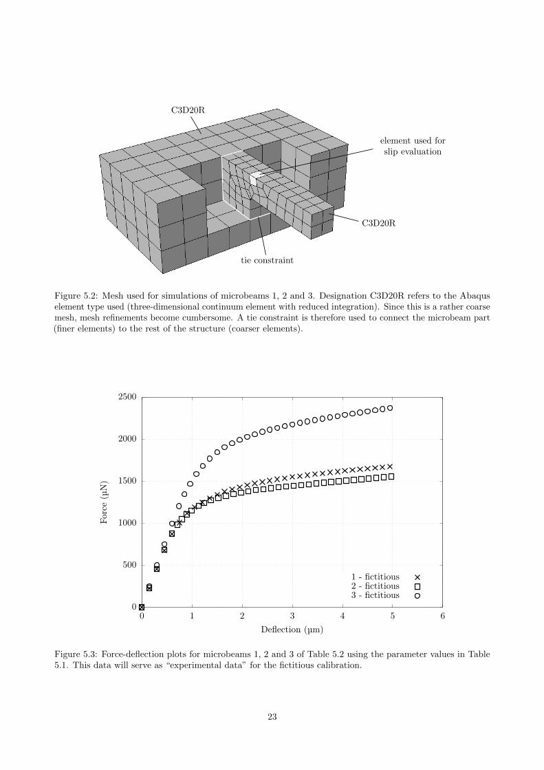
element used forslip evaluation

Figure 5.2: Mesh used for simulations of microbeams 1, 2 and 3. Designation C3D20R refers to the Abaquselement type used (three-dimensional continuum element with reduced integration). Since this is a rather coarsemesh, mesh refinements become cumbersome. A tie constraint is therefore used to connect the microbeam part(finer elements) to the rest of the structure (coarser elements).

0

500

1000

1500

2000

2500

0 1 2 3 4 5 6

Force(µN)

Deflection (µm)

1 - fictitious2 - fictitious3 - fictitious

Figure 5.3: Force-deflection plots for microbeams 1, 2 and 3 of Table 5.2 using the parameter values in Table5.1. This data will serve as “experimental data” for the fictitious calibration.

23

5.2.1 Finding Elastic Parameters C11, C12 and C44

For the calibration of the elastic response, we consider the problem of finding the correct combination orcombinations of parameters C11, C12 and C44. Any solution should give the objective elastic beam stiffnessesfor each one of the three fictitious microbeams. The stiffness quantity can be interpreted as the slope of theelastic loading part in a force-deflection response curve and will be denoted k or F/δ. The F/δ-stiffnesses canalso be altered by the means of changing geometry and/or crystal orientation. However, the geometry andorientation are known for each microbeam and therefore held fixed.

The F/δ-stiffness for the fictitious microbeams 1, 2 and 3 will be denoted k1, k2 and k3, respectively. Thecorresponding “experimental results” can be evaluated from the responses in Figure 5.3 and are given by

k1,fictitious = 1495.31 N/m, k2,fictitious = 1504.30 N/m, k3,fictitious = 1662.05 N/m. (5.2)

Let us introduce the optimization variables s1, s2 and s3 defining the elastic parameters C11, C12 and C44,respectively. These variables will simply scale the reference values of Inconel 718 such that

C11(s1) = s1C11,IN718, C12(s2) = s2C12,IN718, C44(s3) = s3C44,IN718 (5.3)

where subscript “IN718” refers to the corresponding parameter value in Table 5.1. Defining the optimizationvariables like this is mostly a matter of convenience. However, if the optimization variables are of the sameorder, it is also easier to define optimization tolerances.

Now, the three microbeam stiffnesses k1, k2 and k3 are considered to be functions of s1, s2 and s3. We wantto find any combination (s1, s2, s3) that solves system of equations

k1(s1, s2, s3) = k1,fictitious = 1495.31 N/m,

k2(s1, s2, s3) = k2,fictitious = 1504.30 N/m,

k3(s1, s2, s3) = k3,fictitious = 1662.05 N/m.

(5.4)

We known that at least (s1, s2, s3) = (1, 1, 1) is a solution since these variables were used to generate the“experimental data”.

The numerical solution to each one of the equations in (5.4) is plotted in Figure 5.4. These surfaces areobtained from an individual optimization of the variable s3 for 5× 5 grid points in the s1s2-plane. Althoughnot entirely evident from the plot itself, an approximate solution is obtained along a curve where all threesurfaces intersect. Hence, the numerical problem seems to have multiple solutions and it will not be possible touniquely find the elastic parameters.

It is noted that the solution surfaces for microbeam 1 and 2 are very close to each other in Figure 5.4. Theintersection of surfaces for microbeams 1 and 2 will then be very sensitive to variations. Hence, orientations ofmicrobeams 1 and 2 alone are not particularly good choices to solve the problem if real experimental data wereto be used. On the other hand, physical experiments with these orientations could be useful for verificationpurposes. Furthermore, as can be seen in Figure 5.3, the plastic response characteristics may differ. In thisregard, these orientations may provide valuable information.

To summarize, we need to introduce some additional constraint if C11, C12 and C44 should be determinedaltogether. One possibility is to make use of the Zener ratio which characterizes the degree of anisotropy ofcubic crystals [12]. The formula for the Zener ratio ar is given by

ar =2C44

C11 − C12(5.5)

where ar = 1 corresponds to an isotropic crystal. Interpreted in terms of the Zener index, it is possible to find asolution if the degree of anisotropy is provided. This suggests that is might be possible to find a unique solutionby taking a multiaxial response of the microbeam bending into account when calibrating the elastic parameters.

Proceeding to the calibration of the plastic parameters in the next subsection, we set C11, C12 and C44 tothe Inconel 718 reference values in Table 5.1, i.e. using (s1, s2, s3) = (1, 1, 1).

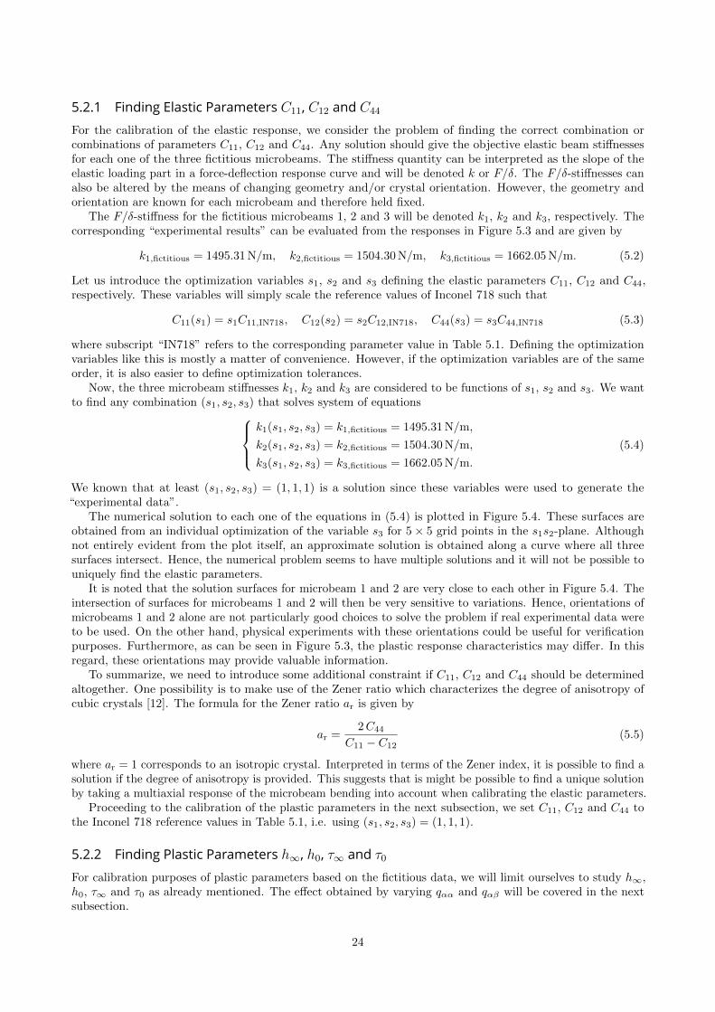
5.2.2 Finding Plastic Parameters h∞, h0, τ∞ and τ0For calibration purposes of plastic parameters based on the fictitious data, we will limit ourselves to study h∞,h0, τ∞ and τ0 as already mentioned. The effect obtained by varying qαα and qαβ will be covered in the nextsubsection.

24

Microbeam 1Microbeam 2Microbeam 3

0.960.98

11.02

1.04s1 0.96

0.981

1.021.04

s2

0.7

0.8

0.9

1

1.1

1.2

1.3

1.4

s3

Figure 5.4: Surfaces for the elastic parameter combinations that results in correct F/δ-stiffness for each one ofthe fictitious microbeams 1, 2 and 3.

In the same way as for the elastic parameters, the optimization variables s6, s7, s8 and s9 are now introducedfor h∞, h0, τ∞ and τ0:

h∞(s6) = s6h∞,IN718, h0(s7) = s7h0,IN718, τ∞(s8) = s8τ∞,IN718, τ0(s9) = s9τ0,IN718. (5.6)

As before, the constants subscripted with “IN718” refer to the Inconel 718 parameter values in Table 5.1.Also, a constraint is added concerning s8 and s9 to ensure that τ∞ ≥ τ0. Without this constraint, the modelbehavior may become strange. Abrupt model behavior changes may be harmful when dealing with numericaloptimization algorithms.

The parameters (s6, s7, s8, s9) are now disturbed from (1, 1, 1, 1). The goal is to calibrate the parameters suchthat the original responses in Figure 5.3 are found again. An optimization is performed using a Nelder-Mead(also called simplex) method in Matlab. Details about how the Abaqus simulations are called iteratively fromMatlab with updated material parameters are presented in Appendix B. The initial guesses for the optimizationvariables are chosen as

s(0)6 = 0.90, s

(0)7 = 1.10, s

(0)8 = 1.10, s

(0)9 = 0.90. (5.7)

Force-deflection plots for these initial guesses may be compared with the “experimental data” in Figure 5.5.The evolution history of the optimization variables when calibrating are plotted in Figure 5.6. The

optimization is terminated with satisfying responses at the values

s(final)6 = 1.0286, s

(final)7 = 1.0582, s

(final)8 = 0.9973, s

(final)9 = 0.9952.

Force-deflection plots with these parameter values are given in Figure 5.5. At this point, variables s8 and s9

(which determine τ∞ and τ0, respectively) both seem to have found an optimal level close to 1. However, thereseem to be lower sensitivities for variables s6 and s7 (determining h∞ and h0). These parameters are stillsubjected to changes at the point of termination although the agreement with “experimental data” in Figure5.5 is very good.

One might suspect that the fictitious plastic optimization problem has a unique solution which meansthat (s6, s7, s8, s9) will approach (1, 1, 1, 1) if the calibration would be continued. However, variables s6 and s7

require greater changes to impact the force-deflection curves than s8 and s9. Hence, s6 and s7 could have beendisturbed more for their initial guess.

5.2.3 Parameters qαα and qαβThe hardening parameters qαα and qαβ are interesting since these, loosely speaking, control the hardeningdistribution among slip systems. Parameter qαα is often referred to as self-hardening whereas qαβ is called

25

0

500

1000

1500

2000

2500

0 1 2 3 4 5 6

Force(µN)

Deflection (µm)

1 - fictitious2 - fictitious3 - fictitious

1 - initial2 - initial3 - initial

0

500

1000

1500

2000

2500

0 1 2 3 4 5 6

Force(µN)

Deflection (µm)

1 - fictitious2 - fictitious3 - fictitious

1 - final2 - final3 - final

Figure 5.5: Initial and final response for the fictitious calibration of plastic parameters h0, h∞, τ0 and τ∞.

26

0.8

0.85

0.9

0.95

1

1.05

1.1

1.15

1.2

0 20 40 60 80 100 120

Opt

imiz

atio

nva

riab

les

Number of iterations

s6 (h∞)

s7 (h0)

s8 (τ∞)

s9 (τ0)

Figure 5.6: Evolution of optimization variables s6, s7, s8 and s9 for the fictitious calibration of the plasticparameters h∞, h0, τ∞ and τ0. The Nelder-Mead method, also known as a simplex method was used forthe optimization through Matlab’s built-in function fminsearch. More information about the calibrationprogramming can be found in Appendix B.

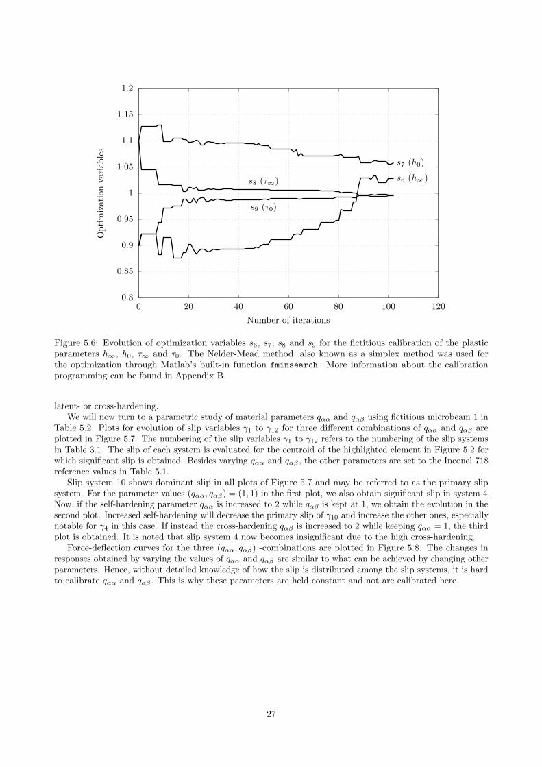
latent- or cross-hardening.We will now turn to a parametric study of material parameters qαα and qαβ using fictitious microbeam 1 in

Table 5.2. Plots for evolution of slip variables γ1 to γ12 for three different combinations of qαα and qαβ areplotted in Figure 5.7. The numbering of the slip variables γ1 to γ12 refers to the numbering of the slip systemsin Table 3.1. The slip of each system is evaluated for the centroid of the highlighted element in Figure 5.2 forwhich significant slip is obtained. Besides varying qαα and qαβ , the other parameters are set to the Inconel 718reference values in Table 5.1.

Slip system 10 shows dominant slip in all plots of Figure 5.7 and may be referred to as the primary slipsystem. For the parameter values (qαα, qαβ) = (1, 1) in the first plot, we also obtain significant slip in system 4.Now, if the self-hardening parameter qαα is increased to 2 while qαβ is kept at 1, we obtain the evolution in thesecond plot. Increased self-hardening will decrease the primary slip of γ10 and increase the other ones, especiallynotable for γ4 in this case. If instead the cross-hardening qαβ is increased to 2 while keeping qαα = 1, the thirdplot is obtained. It is noted that slip system 4 now becomes insignificant due to the high cross-hardening.

Force-deflection curves for the three (qαα, qαβ) -combinations are plotted in Figure 5.8. The changes inresponses obtained by varying the values of qαα and qαβ are similar to what can be achieved by changing otherparameters. Hence, without detailed knowledge of how the slip is distributed among the slip systems, it is hardto calibrate qαα and qαβ . This is why these parameters are held constant and not are calibrated here.

27

0

0.05

0.1

0.15

0.2

0 20 40 60 80 100

0

0.05

0.1

0.15

0.2

0 20 40 60 80 100

0

0.05

0.1

0.15

0.2

0 20 40 60 80 100

γ

Time (s)

Microbeam 1 - qαα = 1, qαβ = 1

γ10

γ4

remaining systems

γ

Time (s)

Microbeam 1 - qαα = 2, qαβ = 1

γ10

γ4

remaining systems

γ

Time (s)

Microbeam 1 - qαα = 1, qαβ = 2

γ10

γ4, remaining systems

Figure 5.7: Evolution of slip variables γ1 to γ12 for three different combinations of qαα and qαβ . The subscriptof the slip variables refer to slip systems in Table 3.1. Simulations are for microbeam 1 with the rest of theparameters set to Inconel 718 values in Table 5.1.

28

0

500

1000

1500

2000

0 1 2 3 4 5 6

Force(µN)

Deflection (µm)

Microbeam 1 - qαα = 1, qαβ = 1Microbeam 1 - qαα = 2, qαβ = 1Microbeam 1 - qαα = 1, qαβ = 2

Figure 5.8: Parametric study for different combinations of (qαα, qαβ) for microbeam 1 with the rest of theparameters set to Inconel 718 reference values in Table 5.1.

29

5.3 Calibration Based on Experimental DataWe now turn to a calibration based on experimental data from the microbeam bending experiments describedin Chapter 2. The geometries and orientations of the three experiment microbeams A, B and C are presentedagain in Table 5.3. Also, recall that the experiments using microbeam A and C unfortunately failed. Theforce-deflection data for the successful microbeam B experiment is plotted in Figure 5.9.

The calibration based on experimental data follows the same pattern as the calibration based on the fictitiousexperiments. In other words, first the elastic parameters C11, C12 and C44 are calibrated and then the plasticparameters h∞, h0, τ∞ and τ0. However, now we only have one experimental response (experiment datafor microbeam B) as compared to three “experiment” responses for the fictitious calibration. A comparisonbetween the activated slip systems in the simulations and the obtained slip lines from experiment images isalso performed for verification purposes.

Since the geometry of the experiment microbeams A, B, C are not the same, different meshes need to beused for these microbeams. The chosen meshes are illustrated in Figure 5.10. The elements that are highlightedare used for slip system verification in Subsection 5.3.3.

In Figure 5.11, finite element model responses for microbeams A, B and C are plotted using the Inconel 718parameters in Table 5.1. The crystal orientations for A, B and C are the same as for the fictitious microbeams1, 2 and 3, respectively. However, comparing Figure 5.3 to Figure 5.11 it may be noted that the beam stiffnessesare greatly affected by the differences in geometry.

Table 5.3: Geometries and crystal orientations for the microbeams used in the experiments. These microbeamsare made of the Allvac 718 Plus superalloy.

Experiment microbeams

Beam Geometry Orientation

L (µm) w (µm) h (µm) r (µm) ϕ1 Φ ϕ2

A 10.45 4.2± 0.04 3.6± 0.03 0.4 302.3◦ 40.7◦ 56.1◦

B 13.0 3.0± 0.06 3.9± 0.04 0.11 79.3◦ 6.8◦ 36.9◦

C 11.8 4.0± 0.04 3.8± 0.06 0.35 247.4◦ 41.9◦ 68.1◦

5.3.1 Finding Elastic Parameters C11, C12 and C44

As before, the problem of determining elastic parameters C11, C12 and C44 that results in the correct F/δ-stiffnessyields a surface of solutions. From the experimental data for microbeam B in Figure 5.9, the F/δ-stiffness isestimated to about 2000 N/m. However, with only a single microbeam, the one denoted B, we need two scalarconstraints in order to uniquely determine C11, C12 and C44. We can now realize that it will not be possible tofind accurate elastic parameters with this experimental data. However, we still may be able to draw usefulconclusions from the results.

We introduce s1, s2 and s3 as in the fictitious calibration, see Equation (5.3). For the first constraint, wesomewhat arbitrarily pick s1 = 1.25 because the microbeam stiffness needs to be drastically increased fromthe Inconel 718 parameters to fit the data. As the second constraint we may assume that Allvac 718 Plus hasthe same Zener index ar as Inconel 718, i.e. ar = 2.71. Imposing these constraints, the solution is obtained as(s1, s2, s3) = (1.250, 1.184, 1.405) or

C11 = 324.5 GPa, C12 = 211.8 GPa, C44 = 154.0 GPa. (5.8)

These values seem very high and inaccurate since the elastic parameters for Allvac 718 Plus are expected to beabout the same as for the Inconel 718. The results will be discussed further in Chapter 6.

5.3.2 Finding Plastic Parameters h∞, h0, τ∞ and τ0With the elastic response calibrated, suitable plastic parameter values for h∞, h0, τ∞ and τ0 are now to befound. The concept of optimization variables s6, s7, s8 and s9 are used again as in Equation (5.6). Using theNelder-Mead method, the evolution of the optimization variables are plotted in Figure 5.12. The final values

30

0

500

1000

1500

2000

0 1 2 3 4 5 6

Force(µN)

Deflection (µm)

Experiment B

Figure 5.9: Force-deflection data from the successful experiment with microbeam B. Images from which thedata is evaluated were acquired once per second. The total time elapsed up to the point of unloading isapproximately 100 seconds.

A

B

C

Figure 5.10: Meshes used for simulations of microbeams A, B and C. All elements are of the type C3D20R.The highlighted elements are used to evaluate slip for the slip lines verification in Subsection 5.3.3.

31

0

500

1000

1500

2000

2500

3000

3500

0 1 2 3 4 5 6

Force(µN)

Deflection (µm)

Beam A - initial parametersBeam B - initial parametersBeam C - initial parameters

Figure 5.11: Response plots for microbeams A, B and C in Table 5.3 using the Inconel 718 reference parametersin Table 5.1.

obtained are

s6 = 3.135, s7 = 1.427, s8 = 0.871, s9 = 1.109 (5.9)

which, if reasonably rounded, correspond to

h∞ = 0.9 GPa, h0 = 8.6 GPa, τ∞ = 521.2 MPa, τ0 = 516.3 MPa. (5.10)

The identified parameter values based on the experimental data are presented in Table 5.4. The correspondingmodel response using these parameters is plotted together with the experiment data in Figure 5.13.

Table 5.4: Calibrated material parameters for Allvac 718 Plus using data from a single microbeam bendingexperiment, the one with microbeam B. The values seem inaccurate and are discussed further in Chapter 6.

Allvac 718 Plus (calibrated)

Elastic parameters Plastic parameters1 2 3 4 5 6 7 8 9 10 11

C11∗ C12

∗ C44∗ γ0

† m† h∞ h0 τ∞ τ0 qαα† qαβ

†

GPa GPa GPa 1/s – GPa GPa MPa MPa – –

324.5 211.8 154.0 0.10 0.017 0.9 8.6 521.2 516.3 1.0 1.0

∗) Value from a non-unique solution, see Subsection 5.3.1.†) Parameter not subjected to calibration, value for Inconel 718 from Reference [8].

5.3.3 Slip Systems VerificationThe experiment beams in Figure 2.3 show clear slip lines. It is interesting to see if the direction of these sliplines can be predicted by slip results from finite element simulations. This can be done by a comparison withdeveloped slip variables γ1 to γ12 for a suitable finite element in the geometry part of interest. A reasonable

32

0.5

1

1.5

2

2.5

3

3.5

0 50 100 150 200

Opt

imiz

atio

nva

riab

les

Number of iterations

s6 (h∞)

s7 (h0)

s8 (τ∞)

s9 (τ0)

Figure 5.12: Evolution of the optimization variables when calibrating the plastic response to fit the experimentdata for microbeam B.

0

500

1000

1500

2000

0 1 2 3 4 5 6

Force(µN)

Deflection (µm)

Experiment BCalibrated model

Figure 5.13: Response curves from the experiment with microbeam B and the corresponding finite elementmodel using the calibrated material parameters in Table 5.4.

33

wα

vαmα

slip linex

yz

slip plane

Figure 5.14: Illustration of a slip plane and corresponding vectors used for identifying slip lines.

assumption is that slip lines belong to a slip plane or a linear combination of slip planes. An illustration isgiven in Figure 5.14.

Consider a vector vα as the direction for a line of intersection between the slip plane corresponding to slipsystem α and any xz-plane. Similarly, let vector wα be the direction for a line of intersection between the slipplane corresponding to slip system α and the xy-plane. The slip plane α has the normal vector mα. Thesedefinitions are illustrated in Figure 5.14.

Vectors vα and wα can be solved for using the equations

mα · vα = mαxv

αx +mα

y vαy +mα

z vαz = 0 (5.11)

andmα ·wα = mα

xwαx +mα

ywαy +mα

zwαz = 0. (5.12)

Since vy = 0 and wz = 0 by definition, the unit vector solutions are given by

vα =

{± (0, 0, 1) for mz = 0,

± (1, 0,−mx/mz) /√

12 +m2x/m

2z for mz 6= 0

(5.13)

and

wα =

{±(0, 1, 0) for my = 0,

±(1,−mx/my, 0)/√

12 +m2x/m

2y for my 6= 0.

(5.14)

We will now try to verify the slip lines obtained in the experiments for microbeams A, B and C by comparingwith the most active slip systems in the simulations. Lines of intersection between the crystal slip planes andthe xz-plane are plotted in Figure 5.15a. These may be compared to the slip lines from the experiment SEMimages in Figure 5.15b. Estimated slip lines from the images are marked with a red line in both Figure 5.15aand 5.15b. Corresponding plots for the xy-plane are presented in Figure 5.16. Evolution of γ1 to γ12 fromsimulations with the initial parameters of Table 5.1 are given in Figure 5.17. These slip variables are evaluatedfor the centroid of the highlighted elements in Figure 5.10.

For the successful experiment with microbeam B, the simulation predicts that system 2 will show most slipfollowed by system 12, see Figure 5.17. Looking from the xz-view in Figure 5.15, we see that the identified redline falls between the lines representing v2 and v12. However, looking from above in Figure 5.16, this is not thecase.

Slip lines for microbeam A and C may not be representative due to failed experiments. As mentioned inChapter 2, it looks like these beams have been subjected to significant torsional deformation. In that case,the slip results are most certainly affected. Studying the slip lines for microbeam A and C in the xz-plane(Figure 5.15), the results do not agree with the simulations (Figure 5.17). However, looking at the slip linesfrom above, i.e. in the xy-plane, the results look better.

The slip system activity from the simulations can not be verified on the basis of Figure 5.15 to 5.17. Noconclusions can be made and it is questionable if this analysis method is reasonable.

34

1, 2, 3

4, 5, 6

7, 8, 9

10, 11, 12

Microbeam A(failed experiment)

x

z

1, 2, 3

4, 5, 6

7, 8, 9

10, 11, 12

Microbeam B x

z

1, 2, 3

4, 5, 6

7, 8, 9

10, 11, 12

Microbeam C (failed experiment)x

z

(a) (b)

Figure 5.15: (a) Lines of intersection between the initial (before deformation) slip planes and the xz-plane, i.e.vectors vα. The numbers refer to the slip systems listed in Table 3.1. (b) SEM images from the experiments.Recall that the experiments with microbeams A and C failed.

35

1, 2, 3

4, 5, 6

7, 8, 9

10, 11, 12

Microbeam A

(failed experiment)

x

y

1, 2, 3

4, 5, 67, 8, 9

10, 11, 12

Microbeam B x

y

1, 2, 3

4, 5, 6

7, 8, 9

10, 11, 12

Microbeam C

(failed experiment)

x

y

(a) (b)

Figure 5.16: (a) Lines of intersection between the initial (before deformation) slip planes and the xy-plane, i.e.vectors wα. The numbers refer to the slip systems listed in Table 3.1. (b) SEM images from the experiments.Recall that the experiments with microbeams A and C failed.

36

0

0.05

0.1

0.15

0.2

0.25

0.3

0 20 40 60 80 100

0

0.05

0.1

0.15

0.2

0.25

0.3

0 20 40 60 80 100

0

0.05

0.1

0.15

0.2

0.25

0.3

0 20 40 60 80 100

γ

Time (s)

Microbeam A - initial parameters

γ10

γ4

remaining systems

γ

Time (s)

Microbeam B - initial parameters

−γ2

γ12, remaining systems

γ

Time (s)

Microbeam C - initial parameters

−γ7

γ8

remaining systems

Figure 5.17: Evolution of slip variables γ1 to γ12 for simulations with microbeams A, B and C. The initialmaterial parameters in Table 5.1 are used for the simulations. Slip data is obtained as a centroid average forthe highlighted elements in Figure 5.10.

37

5.4 Boundary Conditions StudyAs mentioned in Chapter 4, it is not straight forward what boundary conditions that are most representativefor the experiment setup. In Section 5.3 it was observed that the stiffness from the experimental data was muchhigher than for the finite element model. The boundary conditions may slightly affect this stiffness. We willtherefore look at a quick study and compare the force-deflection responses for different boundary conditions.

Some different modeling options with respect to boundary conditions and corresponding responses are shownin Figure 5.18 for microbeam B. The material parameters used are the ones for Inconel 718 in Table 5.1. Theblack bold lines mark the outlines of the faces that are fixed. Model 1 corresponds to the one used for thecalibration. It is seen that the stiffness is barely affected by the model changes. Hence, the discrepancy instiffness between the model and the experimental data can not be explained by nonrepresentative boundaryconditions. Also keep in mind that a refined mesh will lower the force and thereby the stiffness as seen inChapter 4.

Another interesting observation can be made. Since the force-deflection curves are very similar for allmodels, we could switch to one of the smaller models to save computational resources. In this case, model 4seems like a good choice since this response lies closer to the ones of model 1 and 2. However, the simulationtimes are not affected much since these elements do not yield. In other words, the elements at the back partare computationally cheap.

38

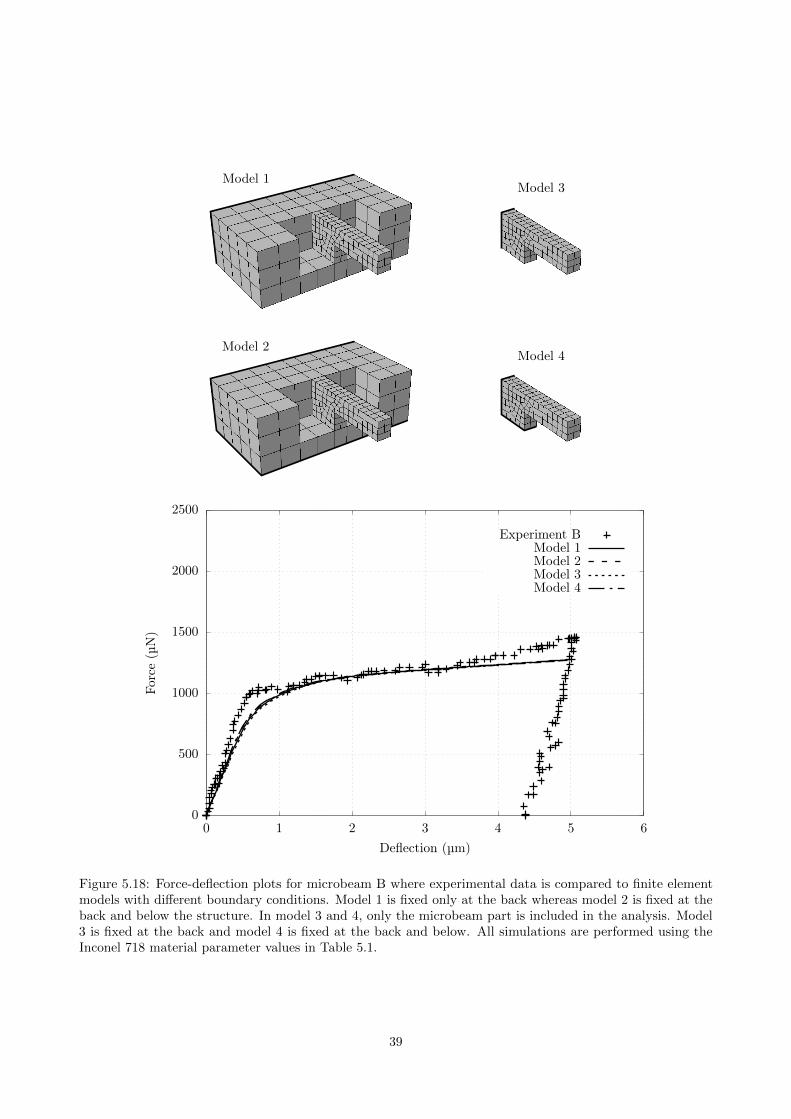
Model 1

Model 2

Model 3

Model 4

0

500

1000

1500

2000

2500

0 1 2 3 4 5 6

Force(µN)

Deflection (µm)

Experiment BModel 1Model 2Model 3Model 4

Figure 5.18: Force-deflection plots for microbeam B where experimental data is compared to finite elementmodels with different boundary conditions. Model 1 is fixed only at the back whereas model 2 is fixed at theback and below the structure. In model 3 and 4, only the microbeam part is included in the analysis. Model3 is fixed at the back and model 4 is fixed at the back and below. All simulations are performed using theInconel 718 material parameter values in Table 5.1.

39

6 Concluding RemarksIn this report, the possibility to calibrate a crystal plasticity model using finite element modeling of microbeambending experiments has been investigated. The microbeam bending experiments are described in Chapter2. The specimens were prepared and the experiments performed at the Department of Physics at Chalmersby Anand Harihara Subramonia Iyer. Three microbeams were made in total with different dimensions andcrystallographic orientation. The microbeams were each milled from a single crystal of the superalloy Allvac718 Plus. Unfortunately, experimental force-deflection data was only obtained for one of the microbeams sincetwo of the experiments failed.

The crystal plasticity model used in this thesis is introduced in Chapter 3. For simplicity, the crystalplasticity model is presented using small strain theory. A corresponding finite strain theory formulation of themodel was used for the simulations in this report. The material user-subroutine for Abaqus was written byMagnus Ekh at the Department of Industrial and Materials Science.

In order to simulate the experiments, a parametrized finite element model of the microbeam structure wasdeveloped. The model is generated from a Python script for Abaqus in which the user can specify relevantgeometry dimensions, material parameters and analysis settings. Python scripts for postprocessing analysisresults, e.g. evaluating force-deflection data, were written as well. More information about the Abaqus Pythonscripts is available in Appendix A.

Some discussion regarding the modeling is presented in the previous chapters. The influence of fixedboundary conditions for different parts of the microbeam structure was investigated in Section 5.4. We foundthat the force-deflection response was not significantly affected by switching to other reasonable boundarycondition choices. Also, the modeling of the displacement load could be implemented with a contact probleminstead of directly prescribing the displacement. However, this would increase the problem complexity andsimulation time. One topic that has not been covered is the influence of variations in geometry and the forceapplication. Physical experiments are never perfect and it is good to be aware of parameters that may be extrasensitive to variations.

Next step was to set up an optimization routine to use for the calibration. The interested reader finds detailsabout the calibration programming in Appendix B. In short, a numerical optimization function in Matlabdrives the calibration of the material model with underlying Abaqus simulations. The model responses fromsimulations are compared to experimental data as an objective function. The material model parameters arethen updated according to some optimization method, in this case the Nelder-Mead method. New simulationsare run and the process continues until some termination criterion is satisfied.

Calibrations of the crystal plasticity model are presented in Chapter 5. Fictitious “experimental data” wasfirst produced by simulations of three different microbeams with same geometry but different crystal orientation.These simulations were performed with a known set of material parameter values. The material parameters werethen disturbed and calibrated to fit the fictitious “experimental data”. Regarding the elastic response (governedby the parameters C11, C12 and C44), we found that the solution was (or at least very close to) non-unique.More response information is needed in order to accurately find all three elastic parameters, force-deflectioncurves are not enough. It is suggested that multiaxial response information could be the solution, analogouslyto measuring the transverse deformation when determining Poisson’s ratio for an isotropically linear elasticmaterial. No attempt was made to include an additional response measure in the calibration process.

The plastic parameters were then calibrated for the fictitious data in Subsection 5.2.2. To limit the calibrationproblem, only four out of eight plastic parameters were considered: h∞, h0, τ∞ and τ0. We observed in thecalibration that the sensitivities w.r.t. force-deflection curves seem to be higher for τ∞ and τ0 when comparedto h∞ and h0. Parameters τ∞ and τ0 found relatively quickly their way back to the original values, see Figure5.6. Anyway, the fictitious plastic calibration problem with regards to only these four parameters seems to bewell-defined.

Parameters γ0, m, qαα and qαβ were not calibrated for different reasons. We realized in the parametricstudy in Subsection 5.2.3 that parameters qαα and qαβ could influence the force-deflection curves in a similarway as the parameters that were calibrated. This could lead to another problem with a non-unique solutionand this is part of the reason why some parameters were omitted from the calibration. However, this couldpotentially be a serious issue worth looking further into in future work. When slip in multiple slip systems areactive, one can argue that it must be important to use accurate values for qαα and qαβ .

In Section 5.3, we looked into a calibration of the material parameters using data from the successful realmicrobeam bending experiment. As for the elastic calibration of the fictitious “experimental data”, no uniquesolution for the elastic parameters could be found. However, the elastic response in the experimental data

40

(Allvac 718 Plus material) was much stiffer than the one predicted from the simulation with the Inconel 718parameter values. Since the elastic parameters of Inconel 718 and Allvac 718 Plus can be expected to besimilar, something seems to be incorrect. We also examined and concluded in Section 5.4, that changing toother, possibly more suited, boundary conditions do not increase the elastic microbeam stiffness much. Theexperimental data may not be accurate enough to calibrate the elastic parameters. Anyway, two constraintswere needed in order to specify values of C11, C12 and C44. As expected, the values of the calibrated elasticparameters turned out to be unrealistically high. We concluded that it may not be reasonable to accuratelycalibrate the elastic parameters from the currently available microbeam bending experiment. More samplescould be used to confirm this and rule out other error sources.

The plastic parameters h∞, h0, τ∞ and τ0 were then calibrated based on the experimental data. The finalcalibrated response in Figure 5.13 seems to be the best fit that this crystal plasticity model can achieve. In thatregard, the calibration was successful. Values for the more sensitive parameters τ∞ and τ0 were rather close tothe Inconel 718 numbers in Table 5.1. However, the hardening parameter h∞ was significantly increased to fitthe experimental data. To be able make any further conclusions we would need to have more experimentaldata to work with.

The specimens show characteristic slip lines after yielding. The slip lines from SEM images of the experimentmicrobeams were compared with the active slip systems in Subsection 5.3.3. No verification or major conclusionscould be made which is a bit worrying. Errors in the analysis or EBSD measurements should not be ruled outas possible explanations. It could also be the case that slip lines are not representative of the most active slipsystems when multiple systems show significant slip.

It should be noted that rather coarse meshes were used throughout all the calibration in the previouschapter. This was a decision based on not only computational resources, but also limitations in Abaqus. Whenperforming numerical optimization tasks very many simulations are needed. Using an implicit finite elementformulation, the scaling obtained with multiple CPU:s or cores is not particularly good. We would of courseprefer results obtained with a finer mesh where it is possible to show fully converged model responses.

There are other issues or error sources not yet mentioned. Statistical scatter is always present when dealingwith experiments and these variations are likely more pronounced on the microscale as compared to themacroscale. The crystal orientations may also not be constant over the whole microbeam which could affectboth the calibration and the slip lines validation.

6.1 Suggestions for Future WorkIn future work it is of course desired to have more experimental data to study. Not only can we expect moreaccurately calibrated parameters, more samples could give an insight into the experimental data accuracyas well. It would also be helpful to have reference experiments with the same setup using another material,e.g. Inconel 718 in this case. It is then preferred to have similar orientations and geometry when comparingmaterials to clearly be able to link differences in the force-deflection response to the material. I would alsorecommend to look into if there are alternatives to the current “spring table” experiment setup to obtain amore accurate force-deflection data.

The elastic parameters will be hard to accurately calibrate using microbeam bending experiments. Firstand foremost, calibration of elastic parameters requires very good data accuracy for small elastic deflectionranges. The data accuracy with the current “spring table” seems to be insufficient. Secondly, the calibrationresults show that more response information is required to determine the elastic parameters. A multiaxialresponse for the microbeam bending would in practice require SEM images from multiple views at the sametime. There may be other types experiments, like tensile bar experiments, which are more suitable for thepurpose of calibrating the elastic parameters. For a bar problem, it could be possible to capture both elongationand transverse deformation from a single view. An SEM image of microbeam B from a top-view after theexperiment is given in Figure 6.1 to illustrate the transverse deformation idea.

If the experimental data accuracy can not be improved for the microbeam bending experiments, I wouldsimply skip the elastic parameters and only focus on the plastic ones. When the calibration of the plasticparameters is performed, one could then choose to only look at the plastic part of the deflection and adjust thedata and model response accordingly.

On the modeling issue with the coarse discretization, it is hard to see a more refined mesh for calibrationjobs. However, one could think of a setup where a first “rough” calibration is performed with a coarser mesh.The calibrated variables may then be used as an initial guess for a calibration with a finer mesh. Regarding

41

Microbeam Btop-view

Figure 6.1: SEM image from a top-view (xy-view) of microbeam B after the experiment. Significant contraction(from a tensile deformation) of the upper part of the microbeam is noted.

the modeling of the force application with the diamond tip, it would be interesting to compare the results ofa prescribed boundary to a contact problem implementation. I expect similar results due to Saint-Venant’sprinciple, but it could be an exercise to perform for completeness.

42

References[1] M. C. Kushan et al. Allvac 718 Plus Superalloy for Aircraft Engine Applications. Recent Advances in

Aircraft Technology, Edited by Dr. Ramesh Agarwal (2012).[2] D. Di Maio and S. G. Roberts. Measuring Fracture Toughness of Coatings Using Focused-ion-beam-

machined Microbeams (2004).[3] O. Kraft, R. Schwaiger, and W. D. Nix. Measurement of Mechanical Properties in Small Dimensions by

Microbeam Deflection (1998).[4] F. Roters et al. Overview of Constitutive Laws, Kinematics, Homogenization and Multiscale Methods

in Crystal Plasticity Finite Element Modeling: Theory, Experiments, Applications. Acta Materialia 58(2010), 1152–1211.

[5] Euler Angles. https://en.wikipedia.org/wiki/Euler_angles. Accessed: 2017-06-13.[6] F. Birch. Finite Elastic Strain of Cubic Crystals (1947).[7] G. Martin et al. A Multiscale Model for the Elastoviscoplastic Behavior of Directionally Solidified Alloys:

Application to FE Structural Computations. International Journal of Solids and Structures 51 (2014),1175–1187.

[8] A. Cruzado et al. Multiscale Modeling of the Mechanical Behavior of IN718 Superalloy Based on MicropillarCompression and Computational Homogenization. Acta Materialia 98 (2015).

[9] Abaqus. Abaqus 6.13 Documentation. 2013.[10] E. Q. Sun. Shear Locking and Hourglassing in MSC Nastran, ABAQUS, and ANSYS. http://web.

mscsoftware.com/events/vpd2006/na/presentations/tech_papers/27.pdf. Accessed: 2017-05-30.[11] M. Ekh, R. Lillbacka, and K. Runesson. A Model Framework for Anisotropic Damage Coupled to Crystal

(visco)Plasticity. International Journal of Plasticity 20 (2004), 2143–2159.[12] Zener Ratio. https://en.wikipedia.org/wiki/Zener_ratio. Accessed: 2017-05-15.

43

A Abaqus Python ScriptingThe Abaqus software provides interfaces via its own Python language, usually called “Abaqus Python” or“Python for Abaqus”, or C++. It is possible to run scripts directly from a terminal, but Abaqus also has acommand line interface (CLI) for the interactive Abaqus Python mode in its graphical user interface (GUI).In fact, all model actions performed in the GUI have an equivalent Python statement or block of statements.There is a “macro recorder” in the Abaqus GUI which produces Python scripts that can be of great help whenwriting own scripts.

Scripting for Abaqus, either using Python or C++, provides good opportunities to automate repetitive tasks.It is also possible to perform tasks that are not possible or very complicated directly in the GUI, like advancedpostprocessing for instance. Two Abaqus Python scripts have been written for the microbeam bending analysis.The first script uses Abaqus to set up a model and produce a corresponding input file. The second scriptperforms a postprocessing job on an output database from an analysis.

A.1 Model Setup ScriptThe model setup script produces a microbeam model from scratch taking various parameters into account. Thefollowing work flow has been adopted in the script:

1. Definition of parameters. These parameters are used for geometry, materials, mesh, load steps and timeincrementation.

2. Setup of materials. The crystal plasticity material model is defined from material parameters. The oxidelayer also needs a material model, if one is to be included.

3. Sketching of geometry. Sketches are made from which the part geometry is created in the next step.

4. Creation of parts. Due to the simple microbeam geometry, it can be created by multiple extrusionstogether with a built-in function for creation of the fillet under the beam. Multiple parts may be created.This is the case if an oxide layer is to be included with another material model.

5. Creation of instances.

6. Meshing of instances.

7. Creation of steps and boundary conditions.

8. Setup of job.

A.2 Postprocessing ScriptA script is also written to postprocess the analysis results and write relevant data to an output file. Informationis written with total time, step time, beam tip deflection and edge reaction force for each time increment.

In Abaqus, a step is an object used to conveniently split up an analysis in natural sequences. These sequencesare typically defined by changes in loads, boundary conditions or interactions. Note that what is often called a“time step” in nonlinear finite element literature is in Abaqus referred to as a time increment, which in turnbelongs to an Abaqus step.

I

B Calibration ProgrammingThis appendix chapter describes how a numerical optimization task may be performed using underlying Abaqussimulations. The methods described here are used to calibrate the crystal plasticity model in this thesis.

Calibration of the parameters in the crystal plasticity model is performed according to Figure B.1. Sincethe Abaqus software lacks a sophisticated calibration module for material model parameters, an externaloptimization code is used instead. This is preferably done using a high-level language suitable for scientificcalculations like Matlab or Python. In this case, Matlab is used. The Nelder-Mead method (also called theSimplex method) is used which is implemented in Matlabs function fminsearch, see Figure B.1.

The first step is to produce an Abaqus input file (text file) for the finite element model. As describedin Appendix A, an Abaqus Python script is written to set up the model and produce an input file. Mostinformation in the input file will remain constant throughout the calibration process.

Next step is to write a function which is passed on as a function handle to fminsearch. This function takesthe variable material parameters (optimization variables) as input arguments and returns an objective functionvalue, see Figure B.1. The operations of this function may be summarized as:

1. Overwrite the Abaqus input file with the new optimization variables. As an example, the linesdefining an isotropic linear elastic material may be given by:

*Material , name=Material -Oxide

*Elastic

275000.0 , 0.25

A straightforward approach is to read all the text file lines and find the one that starts with the string’*Material, name=Material-Steel’. With the index of this line known, one can then replace the linewith the parameters two lines below and overwrite the file.

2. Perform an Abaqus job call with the new input file. This can be done in Matlab using thefunction system, which is used to execute operating system commands:

system(’abaqus job=Job -Microbeam ’)

3. Wait for the job to be completed. Abaqus writes an output database file with extension .odb

containing model information and analysis results. While Abaqus has this output database file openwith write access, a database lock file with extension .lck is present in the working directory. Therefore,before accessing the output database, we need to wait until the lock file is no longer present. A Matlabfunction is written for this purpose. The lock file also remains in the folder if errors are encounteredduring the analysis.

4. Run an Abaqus Python script which postprocesses the output database results. The resultsof interest are then written to an output text file.

system(’abaqus viewer noGUI=microbeam_postprocess.py ’)

5. Wait for the postprocess to be completed. See step 3.

6. Read the output data text file produced in the previous step.

7. Evaluate the objective function value which is then returned.

II

Abaqus/Standard

Abaqus/Viewer

microbeam.odb

results.csv

microbeam.log

(working directory link)

fminsearch pfinal (calibrated values)

pinitial (initial guess)

pk (iteration k)

1. Update microbeam.inpwith parameters pk

2. Run Abaqus job:microbeam.inp

3. Wait for job to becompleted

4. Postprocessmicrobeam.odb

5. Wait for postprocess tobe completed

6. Read results.csv

7. Evaluate objectivefunction value f(pk) andreturn

f(pk)

Figure B.1: Illustration of how the material parameters can be calibrated using optimization code in Matlabwith underlying Abaqus simulations.

III