An Analysis of Finite Volume, Finite Element, and Finite DifferenceMethods Using Some Concepts from Algebraic Topology

Claudio Mattiussi

Evolutionary and Adaptive Systems Team (EAST)

Institute of Robotic Systems (ISR), Department of Micro-Engineering (DMT)

Swiss Federal Institute of Technology (EPFL), CH-1015 Lausanne, Switzerland

plains why it is expedient to use two distinct and dualdiscretization grids, it shows how they must be staggeredIn this paper we apply the ideas of algebraic topology to the

analysis of the finite volume and finite element methods, illuminat- to achieve optimal performance and proposes a techniqueing the similarity between the discretization strategies adopted by for the construction of high order algorithms which complythe two methods, in the light of a geometric interpretation proposed with the physics of the problem on regular and irregularfor the role played by the weighting functions in finite elements.

grids. A final section devoted to an analysis of the discreti-We discuss the intrinsic discrete nature of some of the factors ap-zation strategies adopted by the finite difference methodspearing in the field equations, underlining the exception repre-

sented by the constitutive term, the discretization of which is main- (FD) underlines the absence in the classical version of FDtained as the key issue for numerical methods devoted to field [4] of the distinct geometric flavor of FE and FV, suggestingproblems. We propose a systematic technique to perform this task, how this reflects in the performance of formulas obtainedpresent a rationale for the adoption of two dual discretization grids

with it. New approaches to FD [13, 14] are also brieflyand point out some optimization opportunities in the combinedanalyzed and commentedselection of interpolation functions and cell geometry for the finite

volume method. Finally, we suggest an explanation for the intrinsic For concreteness, in the course of the exposition we willlimitations of the classical finite difference method in the construc- almost always refer to a steady heat conduction modeltion of accurate high order formulas for field problems. problem. The choice of thermostatics was made in order

to present the results in a context which, for its simplicity,should be familiar to the widest possible audience. None-theless, the discussion applies to every field theory whose1. INTRODUCTIONfield equation admits a factorization in the spirit of theone presented in Section 2. Reference [5] shows that aTo solve a field problem by means of the finite elementgreat number of physical equations admit this factoriza-method (FE), we start by partitioning the domain of thetion. Moreover, even if our model problem translates in aproblem into elements and assigning a certain number ofboundary value problem, the analysis performed in thisnodes to each element [1]. The starting point of the finitepaper applies also to problems which translate in initial-volume method (FV) is very similar, but for the introduc-boundary value problems, the extension merely requiringtion of an additional staggered grid of cells, usually definingthe introduction of the necessary time-like geometric ob-one cell around each node [2]. Despite the grid differences,jects.a system of equations fully equivalent to the FV one can

be obtained with FE using as weighting functions the char-acteristic functions of FV cells, i.e., functions equal to unity 2. A DIGRESSION ON EQUATIONSinside the cell and zero outside [3]. Once ascertained thatparticular FE weighting functions can be used to define 2.1. The Factorization of Field EquationsFV cells, we can be tempted to ask if a similar role can be

Let us start by defining the terminology adopted in thisascribed to generic weighting functions. This paper will

paper, considering the case of thermostatics. Apart fromshow that we can answer positively to this question, pro-

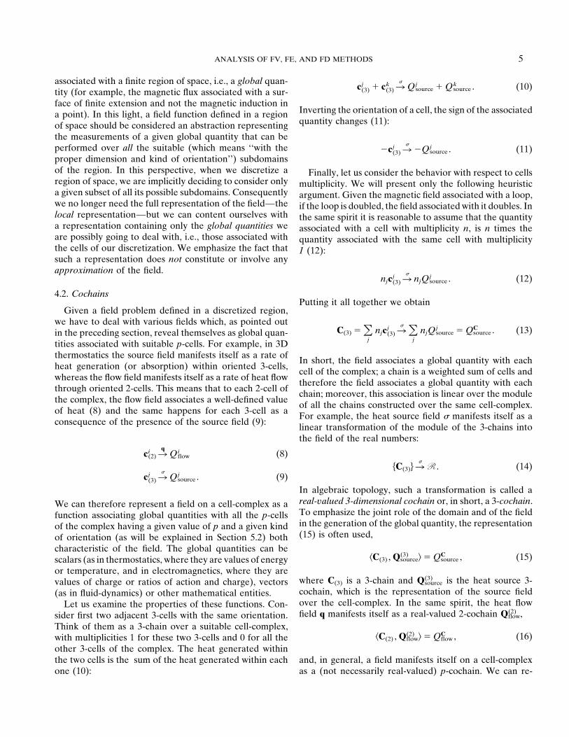
boundary conditions, the field equationvided we recognize that the cells defined by genericweighting functions are not necessarily crisp, but can be

�div(� grad T) � � (1)spread (Fig. 1). The discussion to follow, while showingthe relevance of algebraic topologic concepts in this fieldof investigation, throws some light on the nature of both (� is the thermal conductivity of the medium) constitutes

the link between the unknown field (the temperature T)FE and FV methods and underlines some optimizationopportunities for the latter. In particular, this paper ex- and the given source field (the rate of heat generation �).

1

.

2 CLAUDIO MATTIUSSI

2.2. The Balance Equation

Given a balance equation in differential terms, its dis-cretization amounts to writing it for domains D of finiteextension. For thermostatics the correspondence is

� � div q } Qsource(D) � Qflow(�D),

(differential or local) (discrete or global)(2)

where � stands for ‘‘the boundary of.’’ We will call localthe equations and physical quantities of the differentialcase and global those of the discrete case. Note that thetransition from local to global takes place without anyapproximation error. This happens because the balanceequation does not require for its validity uniform fields,homogeneous materials or any other condition holding ingeneral only in domains of infinitesimal extension. Let usexpress this concept by calling it a topological equation tosuggest an idea of invariance under arbitrary homeomor-phic transformations. For a topological equation, the dis-FIG. 1. FE weighting functions and corresponding crisp and spread

cells. crete version appears therefore as the fundamental one,with the differential statement proceeding from it if addi-tional hypotheses are fulfilled.

It is expedient to factorize the field equation decomposing 2.3. The Constitutive Equationit into three parts: balance equation, constitutive equation,

Contrary to the case of the balance equation it is gener-and kinematic equation (this last name is not standard andally impossible to put in discrete form a local constitutivehas only a mnemonic purpose, inspired by elasticity [1]).equation without limiting its applicability to particular fieldAn expressive representation for the factorization isconfigurations. This happens because a general form for aachieved with the diagram of Fig. 2 where, to allow theconstitutive equation, valid over regions of finite extension,reader to think in terms of a field problem of his choice,can be given only if the field is supposed uniform and theconventional names were assigned to the physical quan-material homogeneous, which is generally not the case.tities.The exact rendering of constitutive equations requires theThis paper will show that the structure of the field equa-use of metrical concepts like length, area, volume, andtion exhibited in Fig. 2 finds a direct correspondence inangle, along with terms describing the properties of thethe strategies adopted by FV and FE to replace Eq. (1)medium.with a system of algebraic equations. In the next three

sections each factor of the field equation is examined in2.4. The Kinematic Equationthis discretization perspective.

The operator appearing in the differential kinematicequation of thermostatics is the gradient, and we knowthat its discrete counterpart involves a simple difference.It is therefore possible to state the kinematic equation indiscrete form:

g � �grad T } G(D) � T(�D),

(differential or local) (discrete or global)(3)

Here G is the global thermal tension, the domain is aline, and its boundary consists of two points. T(�D) is thedifference of two temperatures (this will be considered inFIG. 2. The factorization diagram for the field equation of thermostat-more detail later). Summing up, we can say that the kine-ics, showing the terminology adopted in this paper for the fields and

the equations. matic equation is a topological equation, since there is no

ANALYSIS OF FV, FE, AND FD METHODS 3

3.2. A Formal Notation for Chains

To proceed in our treatment of chains, we need a reason-ably compact notation for them. Let us start by labelingeach oriented cell of the grid with a superscript univocallyidentifying it. The multiplicity with which the cell labeledi appears in a chain will be denoted by ni . With thesechoices we can represent a chain as a formal sum:

C � �i

nici. (4)

This notation has some link with the intuitive idea of com-posing a domain by ‘‘adding’’ its parts. A chain is in fact

FIG. 3. The discretizability of the factors of the field equation.an element of a free module which has the cells as genera-tors and chains generated by a given ensemble of cells canbe added, subtracted, and multiplied by integers, allowingthe algebraic manipulation of domains. In a 3D space theapproximation involved in its discrete rendering. Figure 3formal sum (4) can be used to represent ensembles ofrecapitulates our analysis of the discretizability of eachoriented and weighted volumes, surfaces, lines, and points.term of the factorized field equation.To prevent the use of many names for a unique concept,provided those geometric objects satisfy some additionalcondition (e.g., of being simply connected [7]), topologists3. THE REPRESENTATION OFspeak in all cases of cells, prefixing the name with theDISCRETIZED DOMAINSappropriate dimension number. So volumes become3-dimensional cells—in short, 3-cells—surfaces become3.1. Chains2-cells, lines 1-cells, and points 0-cells. Chains formed with

To give a formal enunciation to the discrete version of p-cells are called p-dimensional chains or p-chains. Thistopological equations, we introduce a tool aimed at the convention will be adopted and the notation adapted ac-representation of discretized domains: the concept of cordingly, writing c(p) for a p-cell and C(p) for a p-chain (5):chain. In FV a balance equation is written for each cell ofthe grid. An implicit orientation of the cells is assumed, C(p) � �

inici

(p) . (5)usually such that the heat generated is to be taken withpositive sign (in contrast with the heat absorbed). We will

In conclusion, chains can be used to represent the discretizedsay that the cell is oriented as a source (opposed to a cellgeometry of a problem.oriented as a sink). If we label a particular oriented cell

as c, it is natural to denote the same cell with opposite3.3. Grids and Cell-Complexesorientation by �c. In this way we can represent an arbitrary

ensemble of oriented cells belonging to the grid, by simply Consider a 3D domain discretized by partitioning it intoattributing them the coefficient 0 (cell not in the ensemble), 3-cells. If the discretization is ‘‘properly performed’’ (in a1 (cell in the ensemble with its orientation unchanged) or topological sense, that can be easily formalized [7]), two�1 (cell in the ensemble with its orientation reversed). Wecan enlarge further the capabilities of this representationby admitting arbitrary integer multiplicities n for cells; thiswill permit, for example, the representation of a multipleloop (Fig. 4). We obtain a collection of cells with integermultiplicity, an object that in algebraic topology is calleda chain with integer coefficients [7].

The concept of chain plays a fundamental role in theestablishment of a point of view comprising both FV andFE, since we can interpret chains as the discrete counter-part of oriented domains with a weighting function definedover them (abridged below as weighted domains). In this FIG. 4. (a) A single loop represented as an ensemble of orientedway the FE’s weighting functions will acquire a geometric lines with multiplicities 0, 1, and �1. (b) A multiple loop requires generic

integer multiplicities.interpretation.

4 CLAUDIO MATTIUSSI

3-cells intersect on a 2-cell or have an empty intersection,two 2-cells intersect on a 1-cell or have an empty intersec-tion and finally two 1-cells intersect on a 0-cell, i.e., a point,or have no points in common. All these cells of variousorders constitute what in algebraic topology is called atridimensional cell-complex, and—when the cells of all or-ders are oriented—a 3D oriented cell complex. The pres-ence of an oriented cell-complex is a prerequisite to thevery definition of chains and was assumed implicitly inthe former discussion. Note that to be a cell-complex, adiscretization grid must satisfy certain conditions (whichexclude, for example, overlapping cells). The term grid is FIG. 5. (a) The boundary of a 2-chain. (b) Appearance of internaltherefore more general than cell-complex and will be used vestiges in the boundary of a 2-chain.to refer to discretized domains in a broader sense.

3.4. The Boundary of a Chainchain composed again by two adjacent 2-cells with compati-

The boundary of a domain is a fundamental notion in the ble orientation but this time with different multiplicity (Fig.enunciation of physical laws and therefore it is advisable to 5b). When we apply to this chain the boundary operator,define this concept for the chains. the common 1-cell receives from its two adjacent cells

The boundary �c(p) of an oriented p-cell c(p) is defined different multiplicities, the sum of which does not vanish.as the (p � 1)-chain composed by the (p � 1)-cells of To the boundary of our 2-chain, belongs in this case a 1-cellthe cell-complex having nonempty intersection with c(p), that we are used to considering internal to the subdomainendowed with the orientation induced on them by c(p) composed by the two 2-cells.[7]. Building on this definition, the linear extension (6) In general, only in the case of p-chains composed byrepresents the procedure to calculate the boundary of a adjacent p-cells with compatible orientation and uniformchain as a combination of its cells’ boundaries. multiplicity, the telescoping property works to cancel all

the internal p-cells, and the boundary operator generatesa (p � 1)-chain which lies on what we are used to consider-

� ��i

nici(p)�� �

ini(�ci

(p)) (6) ing the boundary of the domain individualized by the en-semble of p-cells appearing with nonnull multiplicity inthe p-chain.This defines the boundary operator �, which transforms

The reason for this long digression on a seemingly minorp-chains in (p � 1)-chains and is compatible with the addi-point lies in our desire to interpret the weighted domainstive and the (external) multiplicative structure of chains;as continuous counterparts of chains. To build a completein other words, it is a linear transformation of the modulecorrespondence, it is mandatory to define (at least implic-of p-chains into the module of (p � 1)-chains over theitly) the boundary of a weighted domain. The present resultsame cell-complex:anticipates that with a weighting function that is not con-stant (on its support), the boundary of the corresponding

�C(p)� ��

�C(p�1)�. (7) weighted domain will appear to be spread over thewhole domain.

3.5. Boundaries with Internal Vestiges4. FIELDS AND DISCRETIZED DOMAINSIn this section we will show that the boundary of a chain

has certain peculiarities with respect to the traditional geo-4.1. The Representation of Fields

metric notion of boundary of a domain and that only forparticular chains do the two concepts coincide. FE and FV discretize the domain of the problem; in this

perspective we have reviewed some tools allowing a formalConsider first two adjacent 2-cells (i.e., having a 1-cellof their boundary in common) with compatible orientation description of discretized domains. We need a similar set

of tools to describe the fields over such domains. The ap-(i.e., inducing on the common 2-cell opposite orientations)and both with multiplicity 1 (Fig. 5a). If we apply the proach adopted can be better understood considering that,

from an operative point of view, the continuous representa-boundary operator to this 2-chain, we find that the common1-cell does not appear in the result. This telescoping prop- tion of a field in terms of a field function is but an abstrac-

tion. This appears obvious as soon as we realize that fromerty is a consequence of the opposite orientations inducedon the common 1-cell by the two 2-cells. Now consider a a measurement we always obtain the value of a quantity

ANALYSIS OF FV, FE, AND FD METHODS 5

associated with a finite region of space, i.e., a global quan-cj

(3) � ck(3) �

�Qj

source � Qksource . (10)

tity (for example, the magnetic flux associated with a sur-face of finite extension and not the magnetic induction in

Inverting the orientation of a cell, the sign of the associateda point). In this light, a field function defined in a regionquantity changes (11):of space should be considered an abstraction representing

the measurements of a given global quantity that can beperformed over all the suitable (which means ‘‘with the �cj

(3) ��

�Qjsource . (11)

proper dimension and kind of orientation’’) subdomainsof the region. In this perspective, when we discretize a Finally, let us consider the behavior with respect to cellsregion of space, we are implicitly deciding to consider only multiplicity. We will present only the following heuristica given subset of all its possible subdomains. Consequently argument. Given the magnetic field associated with a loop,we no longer need the full representation of the field—the if the loop is doubled, the field associated with it doubles. Inlocal representation—but we can content ourselves with the same spirit it is reasonable to assume that the quantitya representation containing only the global quantities we associated with a cell with multiplicity n, is n times theare possibly going to deal with, i.e., those associated with quantity associated with the same cell with multiplicitythe cells of our discretization. We emphasize the fact that 1 (12):such a representation does not constitute or involve anyapproximation of the field.

njcj(3) �

�njQj

source . (12)

4.2. CochainsPutting it all together we obtain

Given a field problem defined in a discretized region,we have to deal with various fields which, as pointed out

C(3) � �j

njcj(3) �

� �j

njQjsource � QC

source . (13)in the preceding section, reveal themselves as global quan-tities associated with suitable p-cells. For example, in 3Dthermostatics the source field manifests itself as a rate of In short, the field associates a global quantity with eachheat generation (or absorption) within oriented 3-cells, cell of the complex; a chain is a weighted sum of cells andwhereas the flow field manifests itself as a rate of heat flow therefore the field associates a global quantity with eachthrough oriented 2-cells. This means that to each 2-cell of chain; moreover, this association is linear over the modulethe complex, the flow field associates a well-defined value of all the chains constructed over the same cell-complex.of heat (8) and the same happens for each 3-cell as a For example, the heat source field � manifests itself as aconsequence of the presence of the source field (9): linear transformation of the module of the 3-chains into

the field of the real numbers:

ci(2) �

qQi

flow (8)�C(3)� �

�R . (14)

cj(3) �

�Qj

source . (9)In algebraic topology, such a transformation is called areal-valued 3-dimensional cochain or, in short, a 3-cochain.We can therefore represent a field on a cell-complex as aTo emphasize the joint role of the domain and of the fieldfunction associating global quantities with all the p-cellsin the generation of the global quantity, the representationof the complex having a given value of p and a given kind(15) is often used,of orientation (as will be explained in Section 5.2) both

characteristic of the field. The global quantities can be�C(3) , Q(3)

source� � QCsource , (15)scalars (as in thermostatics, where they are values of energy

or temperature, and in electromagnetics, where they arewhere C(3) is a 3-chain and Q(3)

source is the heat source 3-values of charge or ratios of action and charge), vectorscochain, which is the representation of the source field(as in fluid-dynamics) or other mathematical entities.over the cell-complex. In the same spirit, the heat flowLet us examine the properties of these functions. Con-field q manifests itself as a real-valued 2-cochain Q(2)

flow,sider first two adjacent 3-cells with the same orientation.Think of them as a 3-chain over a suitable cell-complex,

�C(2) , Q(2)flow� � QC

flow , (16)with multiplicities 1 for these two 3-cells and 0 for all theother 3-cells of the complex. The heat generated withinthe two cells is the sum of the heat generated within each and, in general, a field manifests itself on a cell-complex

as a (not necessarily real-valued) p-cochain. We can re-one (10):

6 CLAUDIO MATTIUSSI

phrase all this, saying that cochains constitute a representa-tion for fields over discretized domains. As field functionscan be added and multiplied by a scalar, so can cochainsdefined over a same cell-complex. Collectively all thesecochains constitute a module.

5. THE REPRESENTATION OFTOPOLOGICAL EQUATIONS

5.1. General Remarks

Consider the two topological equations of thermostatics(Fig. 2). In their discrete form, both equations assert theexistence of a relation between a global quantity associatedwith an oriented domain and another global quantity asso- FIG. 6. (a) External orientation for 3-, 2-, 1-, and 0-cells. (b) Internalciated with the boundary of that domain (Eqs. (2) and orientation for 0-, 1-, 2-, and 3-cells.(3)). On a discretized domain, if we represent a volumeas a chain V(3), the source field as a cochain Q(3)

source, andIn conclusion, we have two kinds of orientations forthe flow field as a cochain Q(2)

flow, we can write the balancegeometric objects: those of Fig. 6b are called internal orien-equation of thermostatics astations; those of Fig. 6a are called external orientations.The same distinction holds in every ‘‘well-behaved’’�V(3) , Q(3)

source� � ��V(3) , Q(2)flow�. (17)

n-dimensional ambient space [9]. Note that the symbolwhich gives internal orientation to p-cells gives by defini-

Similarly, the kinematic equation asserts the equality of tion external orientation to (n � p)-cells. This fact permitsthe tension associated with an oriented line and of a combi- the erection in an n-dimensional ambient space of two dualnation of the potentials associated with the two oriented cell complexes, with each p-cell with internal orientationpoints which constitute its boundary. Since the concept of of the first matched by a (n � p)-cell with external orienta-an oriented point may sound unfamiliar to the reader, we tion of the second.shall consider to some greater extent the concept of orien- From the existence of two kinds of orientation followstation. the need of two discretization grids, one with internal ori-

entation and the other with external orientation (the im-5.2. Internal and External Orientation

portance of this distinction of orientations and the benefitsderiving from the adoption of two dual cell-complexes asDeriving the boundary of a cell and writing a topological

equation requires the concept of orientation induced by grids, are usually underestimated [17]). To refer compactlyand unambiguously to them, the former will be called pri-an oriented domain on its boundary. This concept implies

the possibility of comparing the orientation of the domain mary grid or—when the term ‘‘cell-complex’’ applies—primary cell-complex; the latter will be called secondarywith the orientation of the boundary. For example, in a

3D ambient space the source/sink orientation of a 3-cell grid or secondary cell-complex. Correspondingly we willspeak of primary and secondary cells, chains, and cochains.(which is, in fact, an orientation with dichotomic symbols

meaning ‘‘in’’ and ‘‘out’’) can be compared with the Let us consider how this distinction of orientation ap-plies to some familiar case. In 3D thermostatics, the tem-‘‘through’’ direction which constitutes the orientation of

the 2-cells lying on its boundary. To calculate the boundary perature is associated with internally oriented points, thethermal tension with internally oriented lines, the heat flowof a 2-cell oriented with a ‘‘through’’ direction, its boundary

1-cells must be oriented by means of a sense of rotation with externally oriented surfaces, and the heat generationwith externally oriented volumes. In 3D magnetostaticsaround them, and this kind of orientation of a 1-cell can

be compared with that of 0-cells endowed with a tridimen- the vector potential is associated with internally orientedlines, the magnetic induction with internally oriented sur-sional screw-sense, or vortex (Fig. 6a). Similarly, to associ-

ate a thermal tension with a 1-cell, the cell must be oriented faces, the magnetic field with externally oriented lines, andthe charge current with externally oriented surfaces. Noteby means of a running direction along it. The boundary

of such a 1-cell must be 0-cells with source/sink orientation. that a topological equation always involves quantities asso-ciated with domains that, being one the boundary of theThis kind of oriented 1-cell can be the boundary of a 2-cell

oriented by means of a sense of rotation on it and, in turn, other, have the same kind of orientation. Later we willobserve that constitutive equations link quantities associ-this 2-cell can be the boundary of a 3-cell oriented by a

tridimensional vortex (Fig. 6b). ated with domains having different kinds of orientation.

ANALYSIS OF FV, FE, AND FD METHODS 7

We can now resume the discussion concerning the kine-matic equation of thermostatics. If we represent an inter-nally oriented line as a chain L(1), the thermal field as acochain T(0), and the thermal tension field as a cochainG(1), we can write the discrete kinematic equation (3) as

�L(1), G(1)� � ��L(1), T(0)�. (18)

Incidentally, note that since the line induces a source-orientation on its starting point and a sink-orientation onits endpoint, if originally the points are sink-oriented (asis implicit in calculus and, therefore, in the definition of

FIG. 7. The discrete representation of topological equations em-the gradient operator), we haveploying the concept of cochain and the definition of the coboundaryoperator. The left and right columns refer to quantities associated with

��L(1) , T(0)� � Tendpoint � Tstartingpoint . (19) objects endowed with internal and external orientation, respectively.

Due to the fact that in heat theory, the points to which weassociate temperatures are source-oriented, we have in- We can extend the definition of � from single cells tostead generic chains of any order

��L(1) , T(0)� � �(Tendpoint � Tstartingpoint). (20)�C(p�1) , �C(p)� �

def��C(p�1) , C(p)�. (24)

The possibility of this difference in the default orientationEquation (24) defines an operator �, which is called theassigned to points in mathematics and in physics, is thecoboundary operator and transforms p-cochains inreason for the presence of the minus sign in kinematic(p � 1)-cochains (25). It can be shown [7] that it is aequations like g � �grad T in thermostatics, E � �gradlinear transformation of the module of p-cochains into the� in electrostatics, and of many other ‘‘minus’’ signs ap-module of (p � 1)-cochains over the same cell-complex:pearing in textbooks of physics.

5.3. The Coboundary of a Cochain �C(p)� ��

�C(p�1)�. (25)A topological equation asserts the equality of two global

Making use of the definitions of cochain and coboundary,quantities, one associated with a geometric object and thewe can redraw the diagram of the factorized field equationother with its boundary. For example, on a discretized(Fig. 2) with an explicit discrete representation for thedomain we can write the heat balance equation (2) asfields and the topological equations (Fig. 7).

Note that we have defined the coboundary operator�c(3) , Q(3)source� � ��c(3) , Q(2)

flow� �c(3) � Cell complex. (21)without reference to any differential operator. The connec-tion will be established in the next section.We can write this topological equation in a more compact

way by defining a 3-cochain �Q(2)flow which satisfies the

5.4. Coboundary and Differential OperatorsrelationIn vector analysis there are familiar differential opera-

tors that act as the coboundary does. For example, the�c(3) , �Q(2)flow� �

def��c(3) , Q(2)

flow� �c(3) � Cell complex. (22)operator divergence transforms a (vector) field that can beintegrated over oriented surfaces in a (pseudoscalar) field

In other words, the 3-cochain �Q(2)flow associates with each that can be integrated over oriented volumes, allowing the

3-cell the rate of heat flow that the 2-cochain Q(2)flow associ- substitution of

ates with the boundary of that 3-cell. This definition allowsthe restatement of (21) in the simpler form (23), where �

V� dv � �

�Vq ds �V � Domain (26)we no longer need to quote explicitly the p-cells nor to

assert ‘‘for all 3-cells,’’ since both are implicit in the co-chain concept: with (compare with (21) and (23), respectively)

Q(3)source � �Q(2)

flow . (23) � � div q. (27)

8 CLAUDIO MATTIUSSI

The operators curl and gradient act in an analogous way and enforces the corresponding weighted residual equationfor each node n of the grid, endowed with a given weightingfor the transition from oriented lines to oriented surfaces

and from oriented points to oriented lines, respectively. function wn with support dn(3):

Therefore the coboundary operator can be considered asthe discrete counterpart of the three differential operators �

dn(3)

wn div q dv � �dn

(3)

wn � dv �n. (31)grad, curl, div. It indeed satisfies the property � � 0(corresponding to curl grad 0 and div curl 0) and its

The next step is the integration by parts of the left-handconverse which, on a simply p-connected complex, leadsside of (31):to the construction of a ‘‘potential’’ [7]. On a pair of n-

dimensional dual cell-complexes the coboundary operatoracting between p and (p � 1) cochains of the primary �

�dn(3)

wnq ds � �dn

(3)

grad wn q dv � �dn

(3)

wn� dv. (32)complex is the adjoint—relative to a natural duality be-tween cochain spaces (see the Appendix)—of the coboun-

Let us give a geometric interpretation to Eq. (31) whichdary acting between (n � p � 1) and (n � p) cochains ofparallels the obvious one of Eq. (28). Equation (31) pre-the secondary complex (this corresponds, for example, tosents integrations over a domain dn

(3) endowed with athe adjointness of �grad and div relative to the duality ofweighting function; think of this weighted domain as aspaces established by D T � dv and D g q dv). Finally,chain composed by infinitesimal cells with real multiplicity.the very definition of the coboundary guarantees that con-To underline this interpretation we can write (31) in theservation of physical quantities possibly expressed by theformtopological equation is preserved in the discrete equation.

This means that the use of the coboundary operator torender in discrete form the topological equations preserves �

wndn(3)

div q dv � �wndn

(3)

� dv �n. (33)in the discrete operator properties that other approaches—for example, the Support-Operators method [13, 14]—are

In the spirit of the divergence theorem we can write (33)obliged to enforce explicitly.in the formTo complete the parallelism between the coboundary

and the differential operators, we should substitute aweighted volume to V in Eq. (26). We will show in Sections �

�(wndn(3))

q ds � �wndn

(3)

� dv �n. (34)5.5 and 5.7 that integration by parts as is used in FE exactlyfulfills this goal.

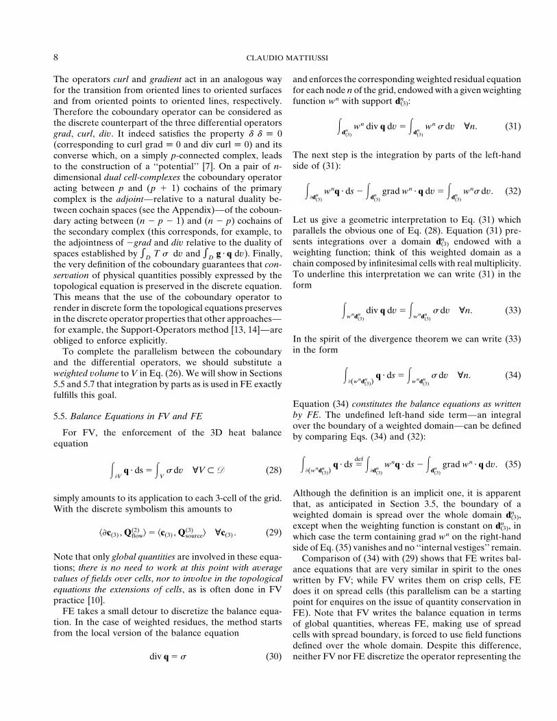
Equation (34) constitutes the balance equations as writtenby FE. The undefined left-hand side term—an integral5.5. Balance Equations in FV and FEover the boundary of a weighted domain—can be defined

For FV, the enforcement of the 3D heat balance by comparing Eqs. (34) and (32):equation

��(wndn

(3))q ds �

def ��dn

(3)

wnq ds � �dn

(3)

grad wn q dv. (35)��V

q ds � �V

� dv �V � D (28)

Although the definition is an implicit one, it is apparentsimply amounts to its application to each 3-cell of the grid.that, as anticipated in Section 3.5, the boundary of aWith the discrete symbolism this amounts toweighted domain is spread over the whole domain dn

(3),except when the weighting function is constant on dn

(3), in��c(3) , Q(2)

flow� � �c(3) , Q(3)source� �c(3) . (29) which case the term containing grad wn on the right-hand

side of Eq. (35) vanishes and no ‘‘internal vestiges’’ remain.Note that only global quantities are involved in these equa- Comparison of (34) with (29) shows that FE writes bal-tions; there is no need to work at this point with average ance equations that are very similar in spirit to the onesvalues of fields over cells, nor to involve in the topological written by FV; while FV writes them on crisp cells, FEequations the extensions of cells, as is often done in FV does it on spread cells (this parallelism can be a startingpractice [10]. point for enquires on the issue of quantity conservation in

FE takes a small detour to discretize the balance equa- FE). Note that FV writes the balance equation in termstion. In the case of weighted residues, the method starts of global quantities, whereas FE, making use of spreadfrom the local version of the balance equation cells with spread boundary, is forced to use field functions

defined over the whole domain. Despite this difference,neither FV nor FE discretize the operator representing thediv q � � (30)

ANALYSIS OF FV, FE, AND FD METHODS 9

actually a superposition of two distinct structures, a cellgrid (usually the primary) and the elements mesh.

5.7. The Role of Integration by Parts in FE

In Section 5.5 an implicit definition for the boundary ofa tridimensional weighted domain was given. By means ofthe identities employed to perform integration by parts,similar formulas for the other cases can be easily obtained.For 3D problems the boundary of weighted 2D and 1Ddomains are implicitly defined by (36) and (37):

��(wndn

(2))A dl �

def ��dn

(2)

wnA dl � �dn

(2)

grad wn A ds (36)

FIG. 8. The two grids and the elements mesh used in FV (the orienta- ��(wndn

(1))T dp �

def ��dn

(1)

wnT dp � �dn

(1)

T grad wn dl. (37)tion of cells is not represented).

In both cases the ‘internal’ part vanishes only if thelocal version of the balance equation. Instead they resortweighting function is constant on dn. The deduction of theboth to the global version of it, and with reason, since acorresponding formulas for 2D and 1D ambient spaces istopological equation applies directly to regions with fi-straightforward.nite extension.

The fundamental role played in FE by the technique ofintegration by parts appears, therefore, as a manifestation5.6. The Two Discretization Grids and theof the necessity to operate with the boundary of spreadElements Meshcells in order to write topological equations. Under this

FV makes use of two staggered discretization grids (Fig. light Eqs. (38)–(40) below play in FE the role played in8) while, apparently, FE does not make use of two grids. In FV by the generalized Stokes theorem (41):fact, FE achieves a similar goal by means of the weightingfunctions which define a spread cell around each node (Fig. �

wndn(3)

div q dv � ��(wndn

(3))q ds (38)1). Note that spread cells relative to different nodes of

the same element, overlap, while the definition of cell- �wndn

(2)

curl A ds � ��(wndn

(2))A dl (39)complexes does not admit cell overlapping. In any case,

even if the characterization of a secondary grid is for themfar from complete, the charge brought against FE of ‘‘re- �

wndn(1)

grad T dl � ��(wndn

(1))T dp (40)

ducing all to nodes’’ must be reconsidered. In many cases,quantities apparently referred to nodes are, in fact, associ- �C(p�1) , �C(p)� � ��C(p�1) , C(p)�. (41)ated with the spread cells surrounding the nodes or to theirboundary. Weighting functions should not be considered

As a final remark, observe that integrals defined overmerely as analytical tools necessary to calculate residues,weighted domains should be considered Stieltjes’ integrals.since they appear endowed with a significant geometricLebesgue made the point in his celebrated lectures [12]meaning.that, owing to its profound geometric meaning, Stieltjes’In addition to the discretization grids, an additional geo-integral—and the implied concept of quantities associatedmetric structure emerges from the distinction that must bewith geometric objects—should be the tool of choice formade between cells and elements. Cells are expedient tomathematical modeling in physics.discrete field representation, for we associate them with

global quantities. Elements, as will become clear in Section6. THE DISCRETIZATION OF6.1, constitute the approximation regions used to performCONSTITUTIVE EQUATIONSthe transition from global quantities to local field represen-

tations, required by the FE and also by the FV discretiza-6.1. General Remarks

tion technique of constitutive equations. In an n-dimen-sional ambient space, elements and primary n-cells often Constitutive equations connect the left and right col-

umns of the factorization diagrams and represent thereforecoincide, but it may happen—especially if the elementshave internal nodes—that each element be composed by a bridge between field variables associated with primary

cells and field variables associated with secondary cells.the union of more than one n-cell (Fig. 11). So we have

10 CLAUDIO MATTIUSSI

Topological equations and constitutive equations together The transition from the representation in terms of formsto the usual one requires the introduction of two referencecompose the complete field equation and we know that

from a discretized formulation of a field problem we usually entities: a metric tensor (from which derives also a unitvolume) and a screw-sense [9].obtain only an approximation to the solution obtainable

(at least potentially) from the local formulation. Therefore, Due to the metrical nature of constitutive equationswe know that a metric tensor must appear in their localhaving stated that topological equations admit exact dis-

crete representation, we can conclude by means of a reduc- representation. A real algebraic relation between thefields—a constitutive tensor composed by the metric tensortio ad absurdum that the discretization of constitutive

equations implies necessarily some approximation in the and some material parameters—is often considered a gen-eral enough representation, but for example, it is not ade-transition from the local to the discrete model. The reasons

behind this inevitable error can be understood by trying quate when the medium involves a nonlocal relation be-tween the fields. The presence of the metric tensor in botha direct discretization of the local constitutive equation of

thermostatics for an isotropic material: the transition between the representations of fields andthe constitutive equations, along with the erroneous as-sumption that constitutive equations are always represent-�g � q. (42)able as algebraic relations, induce some authors to repre-sent both with the same operator �. If this gives an elegantCalling Qflow the rate of heat flow through a secondarymathematical appearance to the formalism obtained, it is2-cell cs

(2) of extension S and G the thermal tension acrossobviously a nonsense that confuses a mathematical manip-a primary 1-cell cp

(1) of extension L, which is the dual ofulation void of physical content, with the transformationcs

(2) and shares its orientation, the simpler discrete relationrepresenting the medium, depriving the constitutive equa-which mimics (42) istions of their physical content. The use of the star operatorto represent constitutive equations and of the metric conju-

�GL

�Qflow

S. (43) gate � of d to write equations of physics are both examples

of this kind of confusion [17].

This relation holds in general only if the material is homo- 6.3. The Structure of Constitutive Equations in FVgeneous, the fields are uniform, cs

(2) is planar, cp(1) is straight,

Consider the constitutive equation of thermostatics. Inand cp(1) is orthogonal to cs

(2). Note that in infinitesimalthe local representation it is a transformation � which linksregions and away from abrupt material discontinuities, allthe field functions g and q and translates the properties ofthese conditions are automatically satisfied (except the or-the medium. As pointed out in the previous section, � isthogonality of cells, which is separately expressed by thea generic transformation, not necessarily representableparallelism of g and q implicit in (42)); this accounts forwith a tensor:the success of local representations in physics.

Equation (43) and its validity conditions remind us thatto write constitutive equations we have to take care—along g �

�q. (44)

with the properties of the medium—of extension, curva-ture, relative position, and other metrical characteristics Correspondingly, in the FV formulation the objects put inof cells. As noted in Section 2.3, constitutive equations relation by the constitutive equation are the two cochainspossess a metrical nature, not merely a topological one. G(1) and Q(2)

flow ,

6.2. Local RepresentationsG(1) �

�Q(2)

flow . (45)A local representation for fields which reflects the natu-

ral association of field quantities with geometric objectsA natural representation of a cochain C(p) is the vector ofendowed with internal and external orientation is given byits values �ci

(p), C(p)�, i.e., the global quantities associatedordinary and twisted differential forms, with the operatorswith the p-cells of the complex over which C(p) is defined.appearing in topological equations represented by the exte-With this representation, if n1 is the number of primaryrior differential d [8]. For example, in thermostatics the1-cells and n2 that of secondary 2-cells, (45) becomespotential can be represented by ordinary 0-forms, the ten-

sion by ordinary 1-forms, the flow by twisted 2-forms, andthe source by twisted 3-forms. For historical reasons therepresentation most widely adopted for fields with scalar �

G1

Gn1

��� �

Q1

Qn2

� (46)global quantities uses instead scalars, (contravariant) vec-tors, and the three differential operators grad, curl, div.

ANALYSIS OF FV, FE, AND FD METHODS 11

which corresponds to n2 functions �i expressing the heatflow through each secondary 2-cell as a function of thethermal tensions across primary 1-cells. The simplest yetnontrivial form that (46) can assume is that of a lineartransformation:

�n1

j�1�i jGj � Qi , i � 1, ..., n2 . (47)

The generic coefficient �i j of (47) expresses the influenceof the thermal tension Gj across the jth primary 1-cellcj

(1) on the rate of heat flow Qi through the ith secondary2-cell ci

(2). There are actually good reasons to put to zerothe greater part of the coefficients �i j; the greater thenumber of zero coefficients in (47), the greater the sparse- FIG. 9. Alternative FV/FE strategies for the discretization of theness of the matrix of the global system of equations. On constitutive equation of thermostatics: (a) 0-cochain approximation fol-the other hand, the greater the number of terms involved, lowed by differential kinematic equation; (b) discrete kinematic equation

followed by 1-cochain approximation.the better we can expect to approximate the local constitu-tive equation with the discrete link �.

complementing the exposition with a couple of elementary6.4. The Structure of Constitutive Equations in FEexamples. We will not undertake the analysis of the compu-

To write FE balance equations we need a local represen- tational properties of the algorithms obtained in these ex-tation of the flow. As a consequence, in the model problem, amples.the objects put in relation by the constitutive equation will To derive the discretized constitutive equation, FV andno longer be the two cochains G(1) and Q(2)

flow, but the FE resort explicitly to the local constitutive equation. Forcochain G(1) and the field function q, a 3D thermostatics problem, the two methods proceed as

follows: an approximation g of the field function g is ob-tained directly from the cochain G(1) or indirectly (via the

G(1) ��

q. (48) differential kinematic equation) from the cochain T(0). Thelocal constitutive equation �g � q is applied to g to obtain

The first term of the link is a discrete representation, an approximate flow density q. Note that from the previouswhereas the second is a local one; the link appears as a step we obtain an actual expression (with the coefficientskind of approximation of a field function. For this reason of T(0) as parameters) for the field function g and we canwe avoid writing the FE link in general form, waiting for apply to this expression a generic transformation, for exam-the definition of cochain approximation to do this. ple a tensor or an integral relation. Given q, FV integrates

it over secondary 2-cells, to obtain the cochain Q(2)flow which

6.5. Strategies for Constitutive Equation Discretizationis necessary for the enforcement of the balance equation�Q(2)

flow � Q(3)source, whereas FE writes the balance equationIn principle, any conceivable method capable of supply-

ing a set of coefficients �i j for Eq. (47) is acceptable as in terms of q, of the source density �, and of the weightingfunctions w which define the shape of the spread cellsdiscretization strategy. For example, one could run a ge-

netic algorithm having the values of the coefficients �i j as (Fig. 9).The final result is the establishment of a direct link ex-parameters and the fitness measure of each individual

linked to the errors resulting from the solution of a given pressing the flow cochain Q(2)flow (for FV) or the flow density

q (for FE) as a function of the unknown cochain T(0). Theensemble of ‘‘adaptation’’ problems. Note that with theapproach presented in this paper, once the domain is dis- fact that neither the intermediate fields g and q, nor the

cochains G(1) and Q(2)flow appear explicitly in the final expres-cretized the rendering of topological equations is univo-

cally determined (in terms of coboundary). Therefore the sion of the balance equations (with the exception of theirrole in the enforcement of boundary conditions, which willonly degree of freedom left is the choice of the discretiza-

tion technique for the constitutive equations. Still, this be considered later) explains why the detailed nature ofthe discretization process and of its main obstacle—thefreedom permits the construction of many algorithms, with

different matrix structures and computational properties. constitutive equation—tend to remain hidden. Indeed,even in FV, an explicit expression for the discrete constitu-In the following pages we will show how to approach in

general terms the discretization of constitutive equations, tive equation linking G(1) to Q(2)flow, is seldom given.

12 CLAUDIO MATTIUSSI

The reader should be aware of the fact that, depending FE, this corresponds to the distinction between nodes, orbetter, spread secondary n-cells, which are interior to theon the theory involved and the phenomena considered,

constitutive equations can link quantities other than ten- element, and spread n-cells which lie on its boundary andare therefore in common with other elements (with thesion and flow (using the conventional names of Fig. 2)

and that more than one constitutive equation can appear exception of nodes lying on the boundary of the problemdomain). To write the balance equation for an interiorsimultaneously in the field equation. Moreover, the quan-

tity occupying the position of the tension in the diagram secondary n-cell (crisp for FV, spread for FE) we needonly the approximate flow density calculated within themight be no longer associated with 1-cells (this happens,

for example, in 3D magnetostatics, where the magnetic element which contains the cell. Conversely, for secondaryn-cells shared between elements, we have to assemble theflux—associated with primary 2-cells—takes the place of

our conventional tension). In each of these cases the dis- contributions derived from the flow densities calculatedwithin all the elements involved. As a consequence, tocretization procedure sketched above, which starts with

the reconstruction from cochains of an approximated field interior cells correspond balance equations involving aminimum number of terms, namely only those correspond-function, still applies with minor changes. The fundamental

step is always the approximation of a continuous represen- ing to the temperatures of the nodes of a single element,whereas a very ‘‘shared’’ cell is characterized by a largetation of a field associated with p-dimensional domains,

based on the information constituted by a p-cochain: an number of nodal temperatures appearing in the corre-sponding balance equation.operation indicated in Fig. 9 with the symbol �

(p), and

called from now on p-cochain-based field function approxi-mation or, concisely, p-cochain approximation. 6.7. p-Cochain Approximation

The idea behind p-cochain approximation is the natural6.6. 0-Cochain Approximation and Equation Assembly

extension to global quantities associated with p-cells, ofthe idea upon which 0-cochain approximation is based.For both FV and FE the approximation based on a

0-cochain is the usual point interpolation. Remember that For example, taking the 1-cochain G(1) as starting point,we have the global quantity ‘‘thermal tension’’ on primarythe kind of mathematical object associated with each

p-cell (a scalar, a vector, etc.) depends on the kind of 1-cells and from this knowledge we want to build an ap-proximation to the field function g . To this purpose, withincochains we are dealing with (scalar-valued, vector-valued,

etc.). For example, in electromagnetics the global quanti- each element we assign an approximation function �e, tak-ing care to select it with the same vectorial nature of gties are scalars and therefore only scalar-valued p-cochain

approximation should be performed, avoiding instead the (note once again that it would be more appropriate torepresent g as a differential 1-form). The number of de-much used interpolations based on nodal values of local

vector quantities like E and H. As done until now, only grees of freedom of �e must be equal to the number ofprimary 1-cells within the eth element. If the approxima-scalar-valued cochains will be considered in the following.

In the case of thermostatics, the 0-cochain we start with is tion function is properly selected in relation to the ele-ment’s shape, the values of G(1) on the primary 1-cellsT (0), i.e., the temperature values on primary 0-cells (which

correspond to the nodes of the FE terminology). Within belonging to the element determine univocally the approx-imating function ge within it. In other words, while ineach element we construct an approximation of the field

function T by means of interpolation functions �e, where 0-cochain approximation we ask the approximating func-tions �e to take the values of T(0) on the primary 0-cellsthe subscript e indicates an approximation holding only

within a particular element. As anticipated in Section 3.3, belonging to the element e, in 1-cochain approximationwe ask the integral of �e on the primary 1-cells belongingelements play the role of approximation regions for the

construction of a continuous representation T for the field to the element e to take the values of G(1) on them. Theextension of this approximation technique to generic p-function. The application to T of the differential kinematic

equation first, and of the local constitutive equation next, cochains is straightforward. The procedure will be clarifiedby the examples in Section 8.is performed element by element. Note that a separate

expression for T, g, and q is available within each element, It is worth stressing that with the point of view adoptedin this paper, the reconstruction of field functions frombut that to write the balance equations we must consider

instead secondary n-cells (n is the dimension of the prob- p-cochains is only expedient to the discretization of theconstitutive equations and is not made with the aim oflem), which can overlap more than one element. In the

case of FV, it is therefore advisable to distinguish between obtaining an expression for field functions over the wholedomain of the problem. In this light, the issue of interele-secondary n-cells which are completely contained in a sin-

gle element (let us call them interior cells), and secondary ment continuity for approximation functions becomes theautomatically satisfied requirement of consistency in then-cells which lie across neighboring elements (Fig. 12). For

ANALYSIS OF FV, FE, AND FD METHODS 13

association of global quantities with p-cells, when this asso- mary 2-cell are the nodes of the element (remember thatall these geometric objects are oriented, even if the orienta-ciation is made by pairs of adjacent elements.

More important than the mere technique of p-cochain tion is not represented in the figure). If we take the routeof 0-cochain approximation, we must define within eachapproximation, is the discussion about the pros and cons

of its adoption (with p 0) in place of 0-cochain approxi- element an interpolating function with the degrees of free-dom appropriate to the four temperature values associatedmation. When—as happens in thermostatics (Fig. 9)—both

strategies are available, the choice is a matter of habit and with the 0-cells. For example, the bilinear polynomial (49)with its four coefficients and its geometric isotropy will do:taste, but there are field problems where there are no

0-cochains to base the approximation on. For example, in3D magnetostatics the quantities which correspond to the pbil(x, y) � a � bx � cy � dxy. (49)potential and the tension in the left column of Fig. 3 arethe line integral of the vector potential A (let us call it �) Obviously, if there are reasons to believe that a differentand the magnetic flux �, respectively. This means that we family of functions (for example, with exponential or ratio-have a 1-cochain �(1) and a 2-cochain �(2), but no nal terms) is particularly suited to a given problem, the0-cochains, to start the interpolation. From a mathematical choice of the approximating functions should comply withpoint of view we can always resort to point-interpolation this additional information. To perform the interpolation,based on nodal values of vector quantities like A and B. we need to know the extent of the elements. Let us callHowever, by so doing we will neglect the correct associa- �x and �y the discretization steps and set a local coordinatetion of quantities with oriented geometric objects, losing system having its origin in a primary 0-cell of the element.its rich geometric content and strong adherence to the Writing Ti, j for T(i �x, j �y), the T(0)-based 0-cochainphysical nature of the problem. Therefore, the widespread approximation performed within the element e, corre-practice of nodal interpolation of local vector quantities sponds to finding a bilinear polynomial Te,bil(x, y) whichshould be avoided and it comes as little surprise the fact satisfies the conditionsthat the idea behind p-cochain approximation is at theheart of some of the techniques adopted by the FE commu- Te,bil(0, 0) � T0,0nity (for example, the use of edge elements [15]), in orderto prevent the appearance of nonphysical terms in the Te,bil(�x, 0) � T1,0

(50)solution. Note also that the p-cochain approximation ap-Te,bil(�x, �y) � T1,1proach avoids the traditional dilemma concerning the loca-

tion of local vector field quantities, since it works with Te,bil(0, �y) � T0,1 .global quantities that we know are associated with p-cells.

This gives6.8. Examples

In this section, the theory expounded will be substanti- Te,bil(x, y) � T0,0 �(�T0,0 � T1,0)x

�x�

(�T0,0 � T0,1)y�y

(51)ated with some example. For simplicity only 2D domainspartitioned in rectangular primary 2-cells which coincide

�(T0,0 � T1,0 � T1,1 � T0,1)xy

�x �ywith elements (Fig. 8) will be considered. Later, the caseof rectangular elements containing more than one primary2-cell will be examined. We strongly emphasize the fact Applying to Te,bil(x, y) the differential kinematic equationthat the theory presented in the previous sections applies g � �grad T and the constitutive equation q � �g wealso to nonorthogonal and to irregular grids, these cases arrive atrequire only an increased bookkeeping effort to takecare—and only in the discretization of the constitutiveequations—of the extension and relative position of cells. qe(x, y) � �(x, y) �(T0,0 � T1,0)

�xIn all cases, particular care must be applied in the place-ment of the discretization grids with respect to discontinu-

�(�T0,0 � T1,0 � T1,1 � T0,1)y

�x �y � i

(52)ities in the properties of the medium and singularities inthe source term—for example, requiring their placementalong the boundaries between elements, so that the inter-

��(x, y) �(T0,0 � T0,1)�ypolation functions do not impose too demanding continu-

ity conditions.With the choice of Fig. 8, element edges coincide with �

(�T0,0 � T1,0 � T1,1 � T0,1)x�x �y � j.

primary 1-cells, while the four primary 0-cells of each pri-

14 CLAUDIO MATTIUSSI

where i and j are the unit base vectors. A relation of this support of the weighting functions. This happens becausethe weighting functions define a spread secondary 2-cell,kind holds within each element; collectively these relations

constitute the FE link between the primary 0-cochain T(0) which in general has a spread boundary. For example,consider Galerkin FE, i.e., FE with weighting functionsand the field function q anticipated in Section 6.4.

In the case of FV, we have to reconstitute the secondary obtained assembling functions of the same kind of theinterpolating functions. With bilinear interpolating func-2-cochain Q(2)

flow from the field function q. To this end wemust perform an integration of q on secondary 1-cells, and tions, the secondary 2-cells are spread over four elements

(Fig. 1)—which we call collectively d(2)—and we havethis requires the definition of their position. This is thesubject of cell optimization that will be discussed in Section8. For the time being, let us just assume that the secondary Qsource

wbild(2)� �

wbild(2)

�(x, y) dx dy (56)2-cells are rectangular, symmetrically staggered with re-spect to primary 2-cells, so that each secondary 1-cell inter-

Qflow�(wbild(2))

� ��(wbild(2))

q(x, y) dl (57)sects orthogonally in the middle a primary 1-cell (Fig. 8).With this choice, a secondary 1-cell lies across two elementsand to calculate the flow Q(i, j)�(h,k) associated with it, we with the following defining relation for the r.h.s. of Eq. (57):need to integrate the approximated flow density q calcu-lated over two adjacent elements. Let us call e1 and e2 thetwo elements involved in the determination of Q(0,0)�(1,0) �

�(wbild(2))q(x, y) dl �

def ��d(2)

wbil(x, y)q(x, y) dland qe1

and qe1the corresponding approximate flow densi-

ties. Of course, the result of the integration depends on� �

d(2)

grad wbil(x, y) q(x, y) dx dy.the function �(x, y) which defines the material. To simplifythe calculations we consider a homogeneous material and (58)�x � �y � �, obtaining the relation

The balance equation isQflow

(0,0)�(1,0)

Qsourcewbild(2)

� Qflow�(wbild(2))

(59)� ��/2

0qe1

(x, y) i dy � �0

��/2qe2

(x, y) i dy (53)

and the final result (with �x � �y � �) once again involves� �(���T0,1 � ��T1,1 � ��T0,0 � ��T1,0 � ��T0,�1 � ��T1,�1).the nine temperatures defined within the four elementswhich constitute the support of the spread secondary 2-cellOnce a similar calculation has been performed for each

1-cell of the secondary grid, the balance equations can be �wbild(2)

�(x, y) dx dy � �(���T�1,1 � ��T0,1 � ��T1,1written. For FV this amounts to equating the heat sourceQsource

c(2)� �c(2), Q(2)

source� within each secondary 2-cell, to thesum of the four heat flows associated with the 1-cells which ���T�1,0 � ��T0,0 � ��T1,0 (60)constitute its (oriented) boundary. In local coordinates

� ��T�1,�1 � ��T0,�1 � ��T1,�1).centered within the cell this means

Obviously in Eq. (55) the source term and the coefficientsQsource0,0 � Qflow

(0,0)�(1,0) � Qflow(0,0)�(0,1)

(54) of the r.h.s. depend on the choice of the shape of thesecondary 2-cell, whereas in Eq. (60) they depend on the� Qflow

(�1,0)�(0,0) � Qflow(0,�1)�(0,0) .

choice of the weighting functions, which define the ‘‘shape’’of the spread 2-cell.We obtain for each secondary 2-cell, the equation

Deciding to take the route of 1-cochain approximation,the first step requires the application of the discrete kine-Qsource

c(2)� �(���T�1,1 � ��T0,1 � ��T1,1 � ��T�1,0

(55) matic equation. With all the primary 0-cells oriented assources, the equation is� 3T0,0 � ��T1,0 � ��T�1,�1 � ��T0,�1 � ��T1,�1).

G(i, j)�(h,k) � Ti, j � Th,k . (61)which involves the nine temperatures associated with the0-cells lying in the four elements which ‘‘share’’ the second-ary 2-cell. The collection of these equations, constitute the In comparison to 0-cochain interpolation, note that by

applying first the topological equation we defer the appear-FV linear system.Writing the FE balance equation requires an integration ance of metrical notions like length and angle. The next

step is the estimation of the field function g based on theof the flow density over all the elements belonging to the

ANALYSIS OF FV, FE, AND FD METHODS 15

cochain G(1). Within each element there are four primary1-cells with their thermal tensions

G(0,1)�(1,1)

G(0,0)�(0,1) G(1,0)�(1,1)

G(0,0)�(1,0)

(62)

FIG. 10. Mixed boundary conditions originate additional constitutivetherefore we can choose as the approximating function a equations. In the thermostatics example considered here, they are duevector-valued function with four coefficients and suitable to the presence of a convective heat exchange across the boundary.symmetry, for example,

plin(x, y) � (a � by)i � (c � dx)j. (63) 7. BOUNDARY CONDITIONS

We consider first the case of boundary conditions whichThe 1-cochain approximation amounts to requiring thatassign some of the unknown (possibly discretized) fieldsthe line integral of the approximating function gc,lin(x, y)along the boundary of the domain. For FV the enforcementperformed on the four primary 1-cells be equal to theof this kind of boundary conditions requires simply thecorresponding thermal tension:positioning along the boundary of the proper kind of pri-mary or secondary p-cells. The global quantities associated��x

0gc,lin(x, 0) i dx � G(0,0)�(1,0) with these cells appear as known terms in the final equa-

tions. In FE the cells and their boundaries can be spread;��x

0gc,lin(x, �y) i dx � G(0,1)�(1,1)

(64)

to include the boundary terms in the equations we mustassure that the weighting functions defining the cells donot vanish along the parts of the boundary where the fields��y

0gc,lin(0, y) j dy � G(0,0)�(0,1)

are assigned. This is usually obtained with the placementof nodes along the boundary, but our analysis shows that��y

0gc,lin(�x, y) j dy � G(1,0)�(1,1) .

this is not mandatory. Note also that the boundary termsare naturally partitioned among bordering cells andnot—as is usually assumed in FE—among borderingThe result isnodes.

To explain how mixed boundary conditions fit in ourgc,lin(x, y) � �G(0,0)�(1,0)

�x�

(G(0,1)�(1,1) � G(0,0)�(1,0))y�x �y � i discretization scheme, we must consider the physical phe-

nomena which originates them. In thermostatics they canappear as a consequence of convective heat exchange

� �G(0,0)�(0,1)

�y�

(G(1,0)�(1,1) � G(0,0)�(0,1))x�x �y � j. across the boundary. We can write the rate of heat ex-

change as(65)

h(T �Dconv� T�) � q �Dconv

, (67)From here we proceed as for 0-cochain interpolation, ob-taining the same final equation. It is worth noting that

where �Dconv are the parts of the boundary where thein the case of FV, we can write explicitly the discreteexchange takes place, h is the coefficient of convective heatconstitutive equation. The prototype of the link is the ex-exchange, and T� is the ambient temperature. To enforcepressionthis kind of boundary condition we have only to treat (67)as a constitutive equation valid on �Dconv (Fig. 10). Thediscretization of the new term proceeds for both FV andFE as described above for constitutive equations.

Qflow(0,0)�(1,0) � ��G(0,1)�(1,1)�

�0G(0,0)�(0,1) �0G(1,0)�(1,1)�

���G(0,0)�(1,0)�

�0G(0,�1)�(0,0) �0G(1,�1)�(1,0)�

���G(0,�1)�(1,�1)

8. CELL OPTIMIZATION

In the examples of Section 6.8, we saw that once theprimary grid, the elements mesh, and the approximationfunctions have been selected, in order to write the balance(66)

16 CLAUDIO MATTIUSSI

equations it is necessary to set the shape of the secondary the temperature distribution within the elements we adoptthe bilinear polynomial (49); we know (Eq. (51)) the result2-cells. In FE, with the interpretation proposed in this

paper, this corresponds to the choice of the weighting func- Te,bil(x, y) of 0-cochain approximation performed withinthe element. For reasons of symmetry, we can aim in ourtions. The options available in the joint selection of shape

and weighting functions are well documented in FE litera- search for higher order approximations in the calculationof the flow, at quadratic polynomialsture, along with the existence of optimal choices for partic-

ular problems.In FV literature, on the other hand, there is seldom pquad(x, y) � a� � b�x � c�y � d�xy � �x2 � �y2. (70)

mention of optimality criteria in the choice of cell shape.Instead, the cells are usually constructed on the basis of We can write the infinitely many polynomials taking thesymmetry considerations and the very adoption of two temperature values of an elements’ four 0-cells asstaggered grid is often considered an oddity, justified aposteriori by the superior performances obtained [11, 16].

T �,�e,quad(x, y) � T0,0 �

(�T0,0 � T1,0)x�x

�(�T0,0 � T0,1)y

�yThe purpose of this section is to show that FV, like FE,can benefit greatly of a properly performed joint selectionof approximation function and cell shape. The examples

�(T0,0 � T1,0 � T1,1 � T0,1)xy

�y �y(71)

to follow are not intended to exhaust the topic of celloptimization in FV, but only to attract interest to the prob-

� �x(x � �x) � �y(y � �y),lem. Therefore we will consider only 2D examples where,mimicking FE, a primary grid, the elements mesh, and the

where the two parameters � and � can take arbitrary val-approximation functions have been arbitrarily set and itues. We must establish if there exists, within the element,remains only to define the shape of secondary 2-cells.a locus which can be taken as a piece of the boundaryMoreover, as in the examples of Section 6.8, all primaryof a secondary 2-cell and such that the flow through it,2-cells and elements are rectangular.calculated from all these quadratic functions, equals theThe basic idea behind our optimization strategy is bor-one calculated with the bilinear function.rowed from polynomial approximation theory and can be

As a first approach, we can look for a curve �(s) (s0 �explained with the following 1D example. Given a reals � s1) lying in the element and satisfying in each pointfunction f(x) defined on an interval [x0, x1], a simple ap-the conditionproximation of it is constituted by a linear interpolation

polynomial flin(x), taking the values f(x0) and f(x1) at thegrad Te,bil(�(s)) n�(s) � grad T �,�

e,quad(�(s)) n�(s) ��, �,endpoints of the interval:(72)

flin(x) � f(x0) �( f(x1) � f(x0))(x � x0)

x1 � x0. (68) where n�(s) is the normal to the curve � in its point of

parameter s. In addition, we ask the curve to constitutethe boundary of a 2-cell, or to contribute to the formationThe derivative of f(x) can be approximated by the deriva-of such a boundary when joined with curves calculated intive of the interpolation polynomial, but since this lastadjacent elements. An alternative is to impose directly,derivative is a constant function, we expect this approxima-instead of the equality of the orthogonal component oftion of f �(x) achieved by f �(x) to be of a lower order,the two gradients in each point of the curve, the equalitycompared to that of f(x) achieved by f(x). It happens,through the curves of the values of the flow calculated withhowever, that all the infinitely many quadratic polynomialsthe two approximating functions: in other words, in placef �

quad(x), taking the values f(x0) and f(x1) in x0, x1,of (72) we can impose

f �quad(x) � f(x0) �

( f(x1) � f(x0))(x � x0)x1 � x0

(69)�

�(s)qbil(�(s)) n�(s) ds

(73)� �(x � x0)(x � x1),� �

�(s)q�,�

e,quad(�(s)) n�(s) ds ��, �,

have a derivative which in the central point xc �(x0 � x1)/2 of the interval takes the same value of the withderivative of the linear interpolation polynomial.

Let us apply this principle to the example of Section qe,bil(x, y) � ��(x, y) grad Te,bil(x, y) (74)6.8, having a primary grid with rectangular 2-cells which

q�,�quad(x, y) � ��(x, y) grad T �,�

e,quad(x, y). (75)coincide with elements (Fig. 8). In this case to approximate

ANALYSIS OF FV, FE, AND FD METHODS 17

This last formulation is more adherent to the spirit ofFV discretization and imposes a lesser constraint on thevariables of the problem but it appears more complex toapply. To keep things simple let us enforce Eq. (72). Givingto the curve � which constitutes the as-yet-unknown cellboundary, the parametric representation

� � x

y(x),(76)

we have the following cartesian expression for n�(s):

n�(x) ��y�(x)i � j�1 � y�(x)2

. (77)

FIG. 11. Grids and elements mesh for biquadratic 0-cochain approxi-Substituting (51), (71), and (77) in (72) we obtain an equa-mation (the orientation of cells is not represented).tion which can be reduced to

�(2x � �x)y�(x) � �(2y(x) � �y) � 0 ��, �. (78)a primary 2-cell but is composed by four of them (Fig. 11).Instead of the four primary 0-cells per element of theThis equation is satisfied for arbitrary �, � withpreceding example, we have now nine primary 0-cells perelement and for this reason the approximation functionsfor temperature within the elements can be biquadraticy(x) �

�y2

. (79)polynomials:

For reasons of symmetry, assigning to � the parametric pbiq(x, y) � a � bx � cy � dxy � ex2 � fy2

(82)representation� gx2y2 � rx2y � sxy2.

� �x(y)

y,(80) We can aim in our search for a better approximation,

at polynomials containing the two cubical terms missingin (82)

we obtain the solution

p�,�cub(x, y) � a� � b�x � c�y � d�xy � e�x2 � f �y2

(83)x(y) �

�x2

. (81) � g�x2y2 � r�x2y � s�xy2 � �x3 � �y3.

Applying 0-cochain approximation based on polynomialsThis means that the axes of symmetry of the primary(82) and (83), we obtain the field functions Te,biq(x, y) and2-cells are optimal loci for the evaluation of the normalT �,�

e,cub(x, y). The optimization equation isflow and, therefore, for the placement of secondary 1-cells.The traditional symmetrically staggered secondary grid

grad Te,biq(�(s)) n�(s) � grad T �,�e,cub(�(s)) n�(s) ��, �with 0-cells placed in the barycentre of primary 2-cells,

(84)adopted tentatively in Section 6.8 (Fig. 8) in this case, isindeed optimal, in the sense that the results obtained with

and gives rise to the equation (referred to a local coordi-these cells using bilinear interpolation polynomials, havenate system with origin in the central primary 0-cell)the same degree of accuracy obtainable interpolating with

complete second-order polynomials. In other words, the�(3x2 � �x2)y�(x) � �(3y(x)2 � �y2) � 0 ��, � (85)adoption of the optimal secondary 2-cells in place of ge-

neric ones, increases by one the rate of convergence ofwhich is satisfied for arbitrary �, � withthe method.

As second example we consider a domain with the sameregular primary grid as the first example but with a different y(x) � �

�y

�3. (86)

elements mesh; now each element no longer coincides with

18 CLAUDIO MATTIUSSI

1-cells on the axes of symmetry of the primary 2-cells(obtaining a regular secondary grid with cells of uniformextension) is not an optimal choice, i.e., will not give, usingbiquadratic interpolation polynomials, the degree of accu-racy obtainable by interpolating with complete third-orderpolynomials. The ensuing absence of improvement in therate of convergence, passing (unawarely) from optimalbilinear to nonoptimal biquadratic interpolation, may ac-count for the widespread—but wrong—feeling that FV,while performing well with low-order interpolation, be-comes less attractive for approximations of higher order.

8.1. Taylor Expansion Applied to the Determination ofFV Optimal Cells

In the spirit of Eq. (72) and (84), we try to determinea locus for the secondary 2-cell boundary such that theapproximation of the component of grad T(x, y) orthogo-nal to it is optimal. Suppose that the curve � which consti-tutes the boundary of the cell, is given the functional repre-sentation (76). Calling n�(x) the normal to � in its genericpoint, we can write the approximation we are trying toachieve as

grad T(x, y) n�(x) � �1i, j��1

ai, j(x, y(x))T(i �x, j �y). (88)FIG. 12. Optimal FV secondary 2-cells (left column) and GalerkinFE spread 2-cells (right column) for the same primary grid and elementsmesh and with the same biquadratic interpolation functions.

Expanding T(x, y) in Taylor series around the genericpoint of � we can write

As before we also have the solutionT(i �x, j �y)

(89)x(y) � �

�x

�3. (87) � �

h,k

1h!k!

(i �x � x)h( j �y � y(x))kT (h,k)(x, y(x)).

Equations (86) and (87) mean that adopting biquadratic Combining (89) with (88), we obtaininterpolation on nine-point square elements (i.e., with�x � �y), we have three kinds of optimal secondary grad T(x, y) n�(x) � �

h,kbi, j(x, y(x))T (h,k)(x, y(x)), (90)

2-cells (Fig. 12): large square cells interior to the element,to which corresponds a 9-point formula; medium-sizedrectangular cells astride the element edges (and therefore where the coefficients bi, j are functions of the ai, js. Substi-shared among two adjacent elements) to which correspond tuting the cartesian expression (77) for n�(x), Eq. (90) be-15-point formulas and, finally, small square cells centered comesin the element vertices (i.e., shared among four elements),to which correspond 25-point formulas. The coefficientsof the formulas can be calculated following the procedure �

T (1,0)(x, y(x))y�(x)

�1 � y�(x)2�

T (0,1)(x, y(x))

�1 � y�(x)2

(91)described in Section 6.8. Proceeding with Galerkin FE withthe same primary grid and elements mesh and adopting � �

h,kbi, j(x, y(x))T (h,k)(x, y(x)).

the same interpolation functions, we obtain again threekinds of secondary 2-cells, with corresponding 9-, 15-, and25-point formulas. Figure 12 shows the optimal FV cells, To obtain a perfect approximation we should achieve

equality in (91). In fact, the best we can do is to imposealong with the corresponding Galerkin FE spread cells,and the ‘‘influence region’’ for each kind of cell. Note that the equality for as many terms of low order as possible.

This gives rise to the system of equationsin this case, to place, as is usually done, the FV secondary

ANALYSIS OF FV, FE, AND FD METHODS 19

and

ky � ��y

�3

a�1,�1(x) �

(96)

b0,0 � 0

b1,0 � �y�(x)

�1 � y�(x)2

b0,1 �1

�1 � y�(x)2

b2,0 � 0

b2,2 � 0

(92)

For reasons of symmetry, to a curve � with a parametricrepresentation (80) there correspond the solutions x(y) �kx � � �x/�3, with their set of coefficients ai, j(x). Withthese curves we can construct the boundaries �ci

(2) of theoptimal secondary 2-cells. Once the optimal cells are found,which is a mixed system of algebraic and differential equa-substituting the calculated coefficients ai, j in (88) we obtaintions. Equations (92) must be solved for the coefficientsthe expression of the optimal approximation of grad T ai, j(x) of Eq. (88) and for the function y(x). To simplifyn�ci

(2)along the boundary of the optimal cells and then wematters, let us look for solutions only among curves parallel

calculate the flux to enforce, finally, the discrete balanceto the x axis, that is, with y(x) � ky , where ky is a constantequation.we must determine. With these choices, (92) becomes

8.2. FV Optimal Cells and FE Superconvergent Points

The introduction of optimal cells should sound familiarto FE practitioners, reminding them of FE optimal flux-sampling or superconvergent points. In fact both conceptshave a common root, but while in FE we look for isolated

b0,0 � 0

b1,0 � 0

b0,1 � 1

b2,0 � 0

b2,2 � 0.

(93) points where the value of the flow density is of higherprecision, in FV we look for a higher precision global flowthrough secondary (n � 1)-cells forming the boundary ofsecondary n-cells. This makes the FV optimization tasklocally easier, because we look for a higher precision onlyfor the component of the flow density (or for its integral)orthogonal to the (n � 1)-cells, but globally much harder,

Writing (93) explicitly in terms of the ai, js we obtain since we look for optimal bounding (n � 1)-dimensionalloci instead of optimal isolated points. Therefore, while FEsuperconvergent points can be easily found for an amplecategory of cell shapes, it may well happen that with somechoice of the primary grid, of the elements mesh, and of

a�1,�1 � � a1,1 � 0

(��x � x)a�1,�1 � � (�x � x)a1,1 � 0

(��y � ky))a�1,�1 � � (�y � ky)a1,1 � 0

(94) the approximation functions, there are no optimal locicapable of constituting the boundary of secondary cells.This is often the case for irregular primary grids, with theoptimization strategy sketched above. In these cases it maybe advisable to try a joint optimization of primary andsecondary grids, or to content oneself with an approxima-which, solved for the ai, js and ky gives two solutions:tion of lower degree for the constitutive equations. Notethat while FE superconvergent points are used to obtainmore accurate numerical data once the calculations havebeen performed, FV optimal cells permit setting an im-proved system of equations prior to the actual executionof numerical calculations.

ky ��y

�3

a�1,�1(x) �(3 � 2�3)(�x � x)x

12 �x2 �y

a1,1(x) �(3 � 2�3)(�x � x)x

12 �x2 �y

(95)9. THE FINITE DIFFERENCE METHODS

FD approaches the discretization problem from a verydifferent perspective than FE and FV. The classical FD

20 CLAUDIO MATTIUSSI

discretization process aims to determine a local discrete of topological equations. This is reflected in the recourseto field functions and metrical tools in the relative discreti-approximation for the operator constituting the complete

field equation. For example, in the case of thermostatics zation step, where global quantities and topological toolsare more appropriate. Consequently the discretization ef-(for simplicity, with homogeneous and isotropic material)

the field equation is forts are partially diverted from the constitutive equations,where they should be focused, in order to select a discreti-zation for the differential operators and to enforce proper-��2T � � (97)ties on it that the (univocally determined) coboundaryoperator satisfies automatically (see Section 5.4).and it is the differential operator �2 that FD tries to write

in discrete terms. Performing on Eq. (97) the discretizationsteps for a nine-point formula on a regular grid with square 10. CONCLUSIONScells of width �x � �y � �, we obtain

We have shown that, introducing the concept of chainand that of spread cell, a strict parallelism can be built�(0, 0)�2 � �(0T�1,1 � 1T0,1 � 0T1,1 � 1T�1,0 � 4T0,0

(98) between the finite element method and the finite volume� 1T1,0 � 0T�1,�1 � 1T0,�1 � 0T1,�1). method. It appears that both methods can be better ana-

lyzed by distinguishing the topological and constitutiveparts of the field equation and recognizing the intrinsicEquation (98), which is the optimal nine-point FD formula,

appears in fact to be the traditional FD five-point formula discrete nature of the topological equations. A conse-quence of this is the realization that the discretization offor the laplacian. In other words, with the FD approach

we are suggested to altogether ignore the four ‘‘corner’’ constitutive equations is the central issue in the constructionof effective discretization schemata and the only placetemperatures. Conversely, the optimal FV nine-point for-

mula (55) (and also the FE nine-point formula (60)) for where the recourse to local representations is fully justified.For topological equations a discrete representation for ge-the same problem and the same discretization grid makes

use of this information, assigning nonzero weights to the ometry, fields, and operators is preferable and, for opera-tors, it is uniquely determined in terms of coboundaries.information carried by these 0-cells. This happens because

the two formulas are aimed at different goals: the FV one This underlines the importance of the correct attributionof physical quantities to geometric objects with appropriateoptimizes the approximation of the constitutive equation,

and therefore of the flow, through the boundary of the orientation and dimension. To the lack of such attributionthe poor performance of high order FD formulas for fieldsecondary cells, while the FD formula constitutes an opti-

mal approximation for the laplacian operator in the central problems and some troubles afflicting FE methods areascribed.point of the patch. This local versus global approach is also

apparent in the l.h.s. source terms of the two equations. The paper also shows how the recognition of the oppor-tunity of employing both internal and external orientationDifferently rephrased, the classical FD approach gives

an optimal solution to a problem which is not the one the constitutes a first argument for the utilization of two dis-tinct discretization grids and it points out that the use ofdiscretization methods for field problems are expected to

face. This is the fundamental weakness of this approach, two dual cell-complexes as grids assures the preservationof the fundamental algebraic properties of topological op-and it explains why it is difficult to obtain well-performing

high-order formulas for field problems with it. Note, on erators. A distinction is made between the discretizationgrids and the elements mesh. It is shown that the latter isthe other hand, that in 1D problems the balance equations

are written for secondary 1-cells, the boundaries of which not a tool devoted to the representation in discrete termsof geometry and fields, but it is instead instrumental toare formed by 0-cells. Therefore, in this case the FD strat-

egy which optimizes on points can coincide with the FV the field function approximation, which is a step in thediscretization of the constitutive equations. A further argu-strategy which optimizes on 1-cell boundaries. In this light

the historical primacy of the FD approach for the discreti- ment supporting not only the distinction of primary andsecondary grids, but also their staggered placement, lieszation of 2D and 3D field problems might be ascribed to

this confusion between two different discretization para- in the minimization thus obtainable of the error implicitin the discretization of constitutive equations.digms and to an unfortunate choice of the wrong one in

the generalization from 1D to higher dimensions. With all this in mind, the choice of the grids and of theelements mesh, the enforcement of boundary conditionsOther kinds of FD schemata—like the support-operator

FD methods [13, 14]—discretize separately in a nonlocal and the whole discretization process can be conducted ina more systematic and efficient way and with close adher-way the first-order differential operators. This approach

would be similar to the one proposed in this paper, but ence to the physical nature of the problems, resulting ingreater insight and better performance.for the failure to acknowledge the intrinsic discrete nature

ANALYSIS OF FV, FE, AND FD METHODS 21

APPENDIX�T(0), �Q(2)

flow� � �Ni�1

Ti ��Mj�1

Ii, jQfj�. (106)

We will show in this appendix that on n-dimensionaldual cell-complexes (primary and secondary complexes, Then we observe that with our choice of dual cell-com-with internal and external orientation, respectively) the plexes and our pairing of orientation and labels of dualcoboundary operator acting on primary (p � 1)-cochains cells, we haveis the adjoint, under a natural duality of cochain spaces,of the coboundary operator acting on secondary I � IT. (107)(n � p)-cochains.

For concreteness we will sketch the proof for the co- Substituting (107) in (106), exchanging running indices,boundary operators appearing in the discretization of 3D and reordering, the identity of (105) and (106) is easilythermostatics (Fig. 7). We can assume without loss of gen- verified. This proves that � is the adjoint of � under theerality that all cells be oriented and univocally labeled in duality of cochain spaces given by (100) and (101).such a way that each pair of dual cells have the samedefault orientation and label. We represent a p-cochain ACKNOWLEDGMENTon a complex with the vector of the global quantities associ-

Many thanks to Gian Guido Folena for his help.ated with the p-cells of the complex:

REFERENCEST(0) � [T1 ... TN], Q(3)source � [Qs

1 ... QsN]

(99)1. D. S. Burnett, Finite Element Analysis (Addison–Wesley, Reading,G(1) � [G1 ... GM], Q(2)

flow � [Qf1 ... Qf

M].MA, 1987).

2. S. Ramadhyani and S. V. Patankar, Solution of the Poisson equation:We put in duality each space of primary p-cochains with Comparison of the Galerkin and control-volume methods, Int. J.

Methods Eng. 15, 1395 (1980).the space of secondary (n � p)-cochains, by means of the3. E. Onate and S. R. Idelsohn, A comparison between finite elementbilinear forms (100) and (101)

and finite volume methods in CFD, Comput. Fluid Dyn. 1, 93 (1992).

4. G. D. Smith, Numerical Solution of Partial Differential Equations(Oxford Univ. Press, London, 1965).�T(0), Q(3)

source� � �Ni�1

TiQsi (100)

5. E. Tonti, On the Formal Structure of Physical Theories (ConsiglioNazionale delle Ricerche, Milano, 1975).

6. P. Penfield Jr. and H. A. Haus, Electrodynamics of Moving Media�G(1), Q(2)flow� � �M

i�1GiQf

i (101)(The MIT Press, Cambridge, MA, 1966).

7. W. Franz, Algebraic Topology (Ungar, New York, 1968).

8. W. L. Burke, Applied Differential Geometry (Cambridge Univ. Press,that are a discrete counterpart ofCambridge, 1985).

9. J. A. Schouten, Tensor Analysis for Physicists (Dover, New York,1989).�T, �� � �

DT� dv (102)

10. J. M. Hyman, R. J. Knapp, and J. C. Scovel, High order finite volumeapproximations of differential operators on nonuniform grids, Phys-�g, q� � �

Dg q dv. (103) ica D 60, 112 (1992).

11. M. Vinokur, An analysis of finite-difference and finite-volume formu-lations of conservation laws, J. Comput. Phys. 81, 1 (1989).We want to prove that

12. H. Lebesgue, Lecons sur l’Integration (Chelsea, New York, 1973),p. 292.

��T(0), Q(2)flow� � �T(0), �Q(2)

flow�, (104) 13. A. A. Samarskii, V. F. Tishkin, A. P. Favorskii and M. Yu. Shashkov,Operational finite-difference schemes, Differential Equations 17,854 (1981).where the overbar distinguishes the coboundary acting on

14. M. Shashkov and S. Steinberg, Support-operator finite-differencethe secondary cell-complex from the one acting on thealgorithms for general elliptic problems, J. Comput. Phys. 118,

primary one. 131 (1995).To show that (104) holds, we start by representing the 15. D. Sun, J. Manges, X. Yuan, and Z. Cendes, Spurious modes in finite-

coboundary operators � and � by means of the incidence element methods, IEEE Antennas Propag. Mag. 37(5), 12 (1995).matrices I and I [7]. 16. N. K. Madsen, Divergence preserving discrete surface integral meth-

ods for Maxwell curl equations using non-orthogonal unstructuredgrids, J. Comput. Phys. 119, 34 (1995).

17. A. A. Dezin, Multidimensional Analysis and Discrete Models (CRC��T(0), Q(2)flow� � �M

i�1��N

j�1Ii, jTj�Qf

i (105)Press, Boca Raton, 1995).