Embed Size (px)
Citation preview

ON FURTHER MODELING OF STIFFNESS AND DAMPING OF
CORRUGATED CARDBOARDS FOR VIBRATION ISOLATION
APPLICATION
A Thesis
Submitted to the College of Graduate Studies and Research
in Partial Fulfillment of the Requirements
for the Degree of
Master of Science
in the
Division of Biomedical Engineering
University of Saskatchewan
Saskatoon, Saskatchewan
Canada
By
Fan Zhang
Copyright Fan Zhang, October 2014. All rights reserved.
i
PERMISSION TO USE
In presenting this thesis in partial fulfilment of the requirements for a Master of Science
degree from the University of Saskatchewan, the author agrees that the Libraries of this
University may make it freely available for inspection. The author further agrees that
permission for copying of this thesis in any manner, in whole or in part, for scholarly
purposes may be granted by the professor or professors who supervised the thesis work or, in
their absence, by the Head of the Department or the Dean of the College in which the thesis
work was done. It is understood that any copying, publication, or use of this thesis or parts
thereof for financial gain shall not be allowed without the author’s written permission. It is
also understood that due recognition shall be given to the author and to the University of
Saskatchewan in any scholarly use which may be made of any material in this thesis.
Requests for permission to copy or to make other use of material in this thesis in whole or
part should be addressed to:
Head of the Department of Biomedical Engineering
University of Saskatchewan
3B48 Engineering Building
57 Campus Drive
Saskatoon, Saskatchewan S7N 5A9
CANADA
ii
ABSTRACT
In a recent study, an environment-friendly material, corrugated cardboard, was used as a
building block for the vibration isolator with a preliminary study. The present thesis was
motivated to advance technology for improving the design of such a corrugated cardboard
vibration isolator with a focus on the modeling of its stiffness and damping.
In particular, this study has performed the following works: (1) improving the FE (finite
element) model of the stiffness of the corrugated cardboards by more accurately identifying
the material parameters in the cardboard material constitutive equation; (2) analyzing the
effect of the error in geometry of the corrugated cardboards in the FE model; (3) developing
the Rayleigh damping model of the corrugated cardboards and evaluating its accuracy.
Several conclusions were drawn from this study: (1) the parameter identification procedure
based on the inverse analysis is feasible for improving the accuracy of the model of the
stiffness of the cardboard. (2) The FE model of the cardboards with a greater in-plane
geometrical deflection has less vertical compressive stiffness. The geometrical deflections of
the corrugated cardboards also change the condition of the contact friction stress and the
compressive deformation. (3) Rayleigh damping model is accurate enough for calculating the
damping of the corrugated cardboards.
The contributions of the thesis include: (1) provision of a more accurate model for the
compressive stiffness the corrugated cardboards, (2) finding that the friction between the
cardboard and the vibrator and the geometrical error of the cardboards have a significant
influence over the accuracy of the FE model, (3) finding that in practice the foregoing
influence can significantly degraded the performance of the cardboards as a vibrator isolator,
and (4) provision of a model for the compressive damping of the corrugated cardboards.

iii
ACKNOWLEDGEMENTS
I would first like to thank my supervisor Professor W.J. (Chris) Zhang for his guidance,
encouragement and advice. His enthusiasm and unlimited zeal on research stimulated me
through my graduate study. He taught me how to think logically and how important it is to be
creative and critical as a researcher. I appreciate all his contributions of time, ideas, and
funding to make my master experience supportive and productive.
I am also thankful to the rest of my committee members, Professor Kushwaha, Lal and
Professor Wu, Fangxiang, your valuable questions, suggestions and comments improved my
work greatly. I would like to thank Jialei Huang for helping me initiate this work and sharing
the relevant experiences and knowledge with me. I would like to thank Louis Roth and
Douglas Bitner for the assistance of setting up experiment test-bed and offering training
patiently. I would like to thank Tim May from Canadian Light Source for providing me the
vacuum pump used in my experiment.
I would also like to thank my family for their support, encouragement, and unconditional
love.
I also extend my gratitude to the friends in my department especially in my group. Thanks to
Xu Wang, Yu Zhao, Xiaohua Hu, Tan Zhang, Bin Han, Lin Cao, Wubin Cheng, Fan Fan,
Sampath Mudduda, Kirk Backstrom to discuss with me about my work. Also thanks to my
friends Zhiming Zhang, Mindan Wang, Zhengshou Yang, Yu Cao for helping me settle down
in Canada when I started my master study.
Finally, I would like to acknowledge the China Council Scholarship (CSC) for partly
providing financial support for my master study.

iv
DEDICATION
To my parents:
Heping Zhang and Yanqiu Li

v
TABLE OF CONTENTS
PERMISSION TO USE .............................................................................................................. i
ABSTRACT ............................................................................................................................... ii
ACKNOWLEDGEMENTS ..................................................................................................... iii
DEDICATION .......................................................................................................................... iv
TABLE OF CONTENTS ........................................................................................................... v
LIST OF FIGURES ............................................................................................................... viii
LIST OF TABLES ..................................................................................................................... x
LIST OF ABBREVIATIONS ................................................................................................... xi
CHAPTER 1 INTRODUCTION ............................................................................................... 1
1.1 Research Background and Motivation ................................................................................. 1
1.2 Brief Review ........................................................................................................................ 2
1.3 Research Objectives and Scope ........................................................................................... 3
1.4 Outline of the Thesis ............................................................................................................ 4
CHAPTER 2 LITERATURE REVIEW .................................................................................... 5
2.1 Introduction of Corrugated Cardboard................................................................................. 5
2.2 Finite Element Modeling of the Corrugated Cardboard ...................................................... 8
2.2.1 Material and mechanical properties ........................................................................... 8
2.2.2 Element .................................................................................................................... 11
2.2.3 Geometry ................................................................................................................. 11
2.2.4 Contact Problem ...................................................................................................... 12
2.2.5 Impact and Vibration Problem ................................................................................. 13
2.2.6 Compression Problem .............................................................................................. 14

vi
2.3 Vibration Isolation ............................................................................................................. 18
2.4 Conclusion ......................................................................................................................... 20
CHAPTER 3 DETERMINATION OF CONSTITUTIVE PARAMETERS ........................... 21
3.1 FE Model ........................................................................................................................... 21
3.1.1 Element .................................................................................................................... 21
3.1.2 Nonlinearity ............................................................................................................. 22
3.1.3 Contact problems ..................................................................................................... 22
3.2 Constitutive law ................................................................................................................. 23
3.3 Experimental Setup ............................................................................................................ 27
3.4 Parameter identification procedure .................................................................................... 28
3.4.1 Design variables (DVs) ............................................................................................ 28
3.4.2 Constraint ................................................................................................................. 36
3.4.3 Objective variables (OVs) ....................................................................................... 36
3.4.4 Optimization method ............................................................................................... 37
3.4.5 Optimization Result ................................................................................................. 39
3.5 Results and discussion ....................................................................................................... 44
3.6 Conclusion ......................................................................................................................... 45
CHAPTER 4 MANUFACTURING IMPERFECTION ANALYSIS OF CORRUGATED
CARDBOARDS ...................................................................................................................... 46
4.1 Introduction ........................................................................................................................ 46
4.2 The Modified FEM Model of the Cardboard ..................................................................... 47
4.3 Modeling of Friction between the Cardboard and Equipment........................................... 49
4.4 Conclusions ........................................................................................................................ 52
CHAPTER 5 MODELING OF THE DAMPING IN CORRUGATED CARDBOARDS ..... 54
5.1 Introduction ........................................................................................................................ 54
5.2 The Rayleigh Damping Model........................................................................................... 54

vii
5.3 Test-bed for determining 𝛇 and 𝛚 .................................................................................... 55
5.4 Verification of the Damping Model ................................................................................... 58
5.4.1 Layer of the cardboard system at the resonance frequency ..................................... 59
5.4.2 Vibration Test .......................................................................................................... 60
5.4.3 Comparison .............................................................................................................. 61
5.5 Conclusion ......................................................................................................................... 62
CHAPTER 6 CONCLUSION AND FUTURE WORK .......................................................... 63
6.1 Overview ............................................................................................................................ 63
6.2 Contributions...................................................................................................................... 64
6.3 Future Work ....................................................................................................................... 65
REFERENCES ........................................................................................................................ 66

viii
LIST OF FIGURES
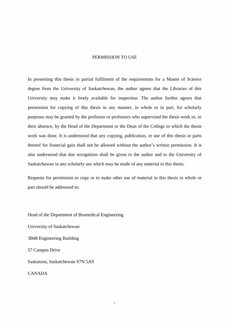
Figure 1.1 Example of vibration isolators under equipment
(http://www.vibrationmountsindia.com/Vibration-Isolation-Mounts-Turret-Punch-Press.ht
ml) ......................................................................................................................................... 1
Figure 2.1 Corrugated cardboard (box and the enlarged image for an edge).......................................... 5
Figure 2.2 Corrugated cardboards with different wall constructions ...................................................... 6
Figure 2.3 The corrugating procedure of a single wall corrugated board. (Allansson and Svärd 2001) 7
Figure 2.4 Three principal directions of the orthotropic cardboard (Nordstrand 2003).......................... 7
Figure 2.5 Typical strain-stress curves of corrugated cardboards under tensile test (Hammou et al. 2012)
.............................................................................................................................................. 9
Figure 2.6 Different flute profiles in FE models (Carlsson et al. 2001) ............................................... 12
Figure 2.7 (a) Actual profile; (b) Sine profile and (c) Saw-tooth profile in FE model (Biancolini 2005)
............................................................................................................................................ 12
Figure 2.8 One-unit corrugated cardboards specimens for (a) FCT and (b) CMT (Lu, Chen, & Zhu,
2001) ................................................................................................................................... 15
Figure 2.9 Comparison between the calculated results and the experimental results (Lu et al. 2001) . 16
Figure 2.10 Comparison between solutions obtained by analytic model, FE model and experiment
(Krusper et al., 2008) .......................................................................................................... 17
Figure 2.11 Comparison of the experimental results and FEM results (Huang 2013) .......................... 18
Figure 2.12 The schematic diagram for a Single-degree of freedom vibration system ........................ 19
Figure 3.1 The geometry of the shell 181 element(ANSYS Inc. 2004) ................................................ 21
Figure 3.2 Geometry of the type-C cardboard ...................................................................................... 27

ix
Figure 3.3 The typical force-displacement curve in compressive experiment ...................................... 28
Figure 3.4 The force-displacement curves with different Shear moduli ............................................... 32
Figure 3.5 The force-displacement curves with different tangent moduli ............................................ 34
Figure 3.6 The force-displacement curves with different Rxx ............................................................. 35
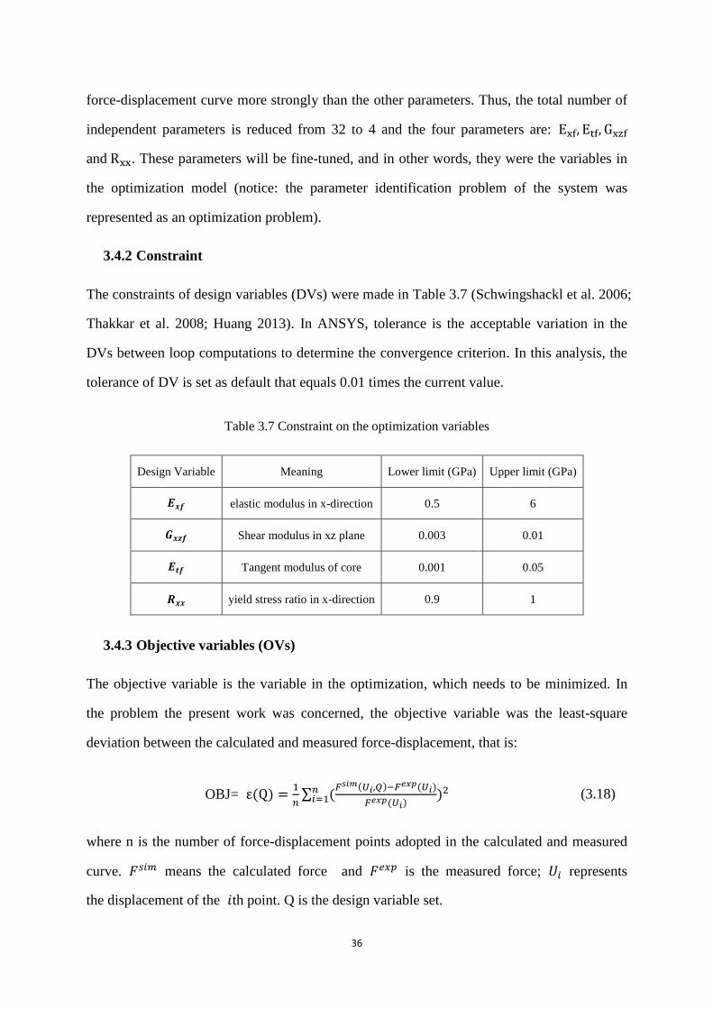
Figure 3.7 convergence behaviors of (a) objective function; (b) Exf;(c) Gxzf; (d) Etf; (e) Rxx ......... 42
Figure 3.8 Objective function results of sweep iterations for each design variable (a) Exf; (b) Gxzf;
(c) Etf; (d) Rxx .................................................................................................................... 44
Figure 4.1 A compressed cardboard sample with transverse shear deformation .................................. 46
Figure 4.2 Free-edge boundary conditions ........................................................................................... 47
Figure 4.3 Geometry of the cross section with the imperfect flute ....................................................... 48
Figure 4.4 Force-displacement curves of the FE models of corrugated cardboard with perfect flute and
imperfect flutes ................................................................................................................... 48
Figure 4.5 Typical deformed shape during compression calculation on imperfect-flute model (5%
deflection) ........................................................................................................................... 49
Figure 4.6 Boundary conditions with the cardboard system under the compression and subject to sliding
between the top surface of the linear and the test head or equipment to be isolated .......... 50
Figure 4.7 Contour of the contact friction stress between the upper liner and the upper platen ........... 51
Figure 4.8 Calculations with different friction coefficients .................................................................. 52
Figure 5.1 (a) Test-bed for damping measurement of the cardboard (b) Vibration exciter .................. 56
Figure 5.2 Function diagram of the test-bed ......................................................................................... 56
Figure 5.3 Typical result of the transmissibility vs frequency .............................................................. 57
Figure 5.4 (a) the test-bed for displacement measurement in the pump-cardboard-ground vibration
system (Huang 2013) (b) the signal flow of the test. .......................................................... 58
Figure 5.5 Measurement results ............................................................................................................ 61

x
LIST OF TABLES
Table .................................................................................................................................. Page
Table 2.1 Specification for Corrugated Flutes (ASTM standard 2007) .................................................. 6
Table 2.2 Stress matrix and strain matrix ............................................................................................... 8
Table 2.3 The most commonly used determination method of material parameters in literature ......... 10
Table 3.1The parameters in the constitutive law of the model of the cardboard .................................. 26
Table 3.2 Geometry of the corrugated cardboard specimen (mm) ....................................................... 27
Table 3.3 Sensitivity of In-plane Young’s moduli in comparison calculations .................................... 30
Table 3.4 Sensitivity of Shear moduli in comparison calculations ....................................................... 32
Table 3.5 Sensitivity of Tangent moduli in comparison calculations ................................................... 33
Table 3.6 Sensitivity of Rxx in comparison calculations ..................................................................... 35
Table 3.7 Constraint on the optimization variables .............................................................................. 36
Table 3.8 The best design set obtained from the sub-problem optimization process compared with the
original parameter set .......................................................................................................... 40
Table 3.9 The best design set obtained from the sweep analysis compared with the original parameter
set ........................................................................................................................................ 42

xi
LIST OF ABBREVIATIONS
AEDL Advanced Engineering Design Laboratory
FE Finite Element
FEM Finite Element Method
FCT Flat Crush Test
CMT Concorra Medium Test
MD Machine Direction
CD Cross Direction
ZD Through-thickness Direction
MPC Multi-point Constraint
DOF Degree of Freedom
APDL Parametric Design Language
DV Design variable
SV State Variable
OV Objective variable
1
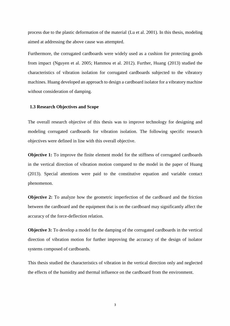
CHAPTER 1 INTRODUCTION
1.1 Research Background and Motivation
Vibration of equipment in industry is usually undesirable which will make noise, reduce
performance or damage equipment potentially. Motorized equipment such as pumps mounted
on a solid structure or to a floor will transfer energy to the structure or to the floor in the form
of vibration. Vibration isolators installed on the building structure are commonly used by
engineers to reduce the harmful effect of vibration caused by the equipment. An example is
shown in Figure 1.1.
Figure 1.1 Example of vibration isolators under equipment
(http://www.vibrationmountsindia.com/Vibration-Isolation-Mounts-Turret-Punch-Press.html)
Any vibration isolator is essentially a system that has stiffness and damping properties.
Stiffness represents the ability of a system to resist deformation along the direction where an
external force or moment is applied. Damping represents the ability of a system to dissipate
the energy in the system (Rao and Horton 2003). Stiffness and damping properties are the

2
two most important properties of a vibration isolator. Accurate modeling of them is important
to the design of the isolator.
There are various types of materials to serve as a physical body of an isolator, for example,
wood, felt, rubber, paperboard, iron, etc. In our research group, Huang (2013) pioneered the
study of an environment-friendly material, corrugated cardboard, for vibration isolator. In his
work, the finite element (or FE) modeling of the stiffness of the cardboards was studied.
Huang (2013) concluded that the FE model of the stiffness can be further improved, which
was a motivation for the present thesis. Further, Huang (2013) did not include the damping in
the design of the cardboard isolator, which was studied in this thesis.
1.2 Brief Review
In the past three decades, the finite element method (FEM) has been widely applied for
analyzing the mechanical properties of the sandwich structures under various conditions of
bending, shearing, tension, compressing and dynamic behavior. The model established with
FEM was able to capture the complex property of isotropic and orthotropic materials and the
contact problem. Most of the previous studies on the static stiffness property of corrugated
cardboards with FEM concerned bending, buckling or shearing behavior. To the best effort of
the author, only three references (Huang, 2013; Krusper et al. et al.2008; Lu et al. 2001) were
found, which studied the through-thickness compressive behavior of corrugated cardboard by
FEM, at least to the writer’s best knowledge. However, their models did not agree well with the
experimental results. In the paper of Lu et al. (2001) and Krusper et al. (2008), there is a
relatively big gap between the calculated results and the experimental results. The peak of the
yield point was not accurately predicted. The model of Huang (2013) improved model
accuracy, with the error of 7.28% between the calculated results and the experimental results.
The cause of the errors with the Huang’s model may likely be the following: (1) the material
parameters are not quite accurate due to the measurement limitations (Huang, 2013); and (2)
the asymmetrical geometry and the frictional shear stress are presented during the compressive
3
process due to the plastic deformation of the material (Lu et al. 2001). In this thesis, modeling
aimed at addressing the above cause was attempted.
Furthermore, the corrugated cardboards were widely used as a cushion for protecting goods
from impact (Nguyen et al. 2005; Hammou et al. 2012). Further, Huang (2013) studied the
characteristics of vibration isolation for corrugated cardboards subjected to the vibratory
machines. Huang developed an approach to design a cardboard isolator for a vibratory machine
without consideration of damping.
1.3 Research Objectives and Scope
The overall research objective of this thesis was to improve technology for designing and
modeling corrugated cardboards for vibration isolation. The following specific research
objectives were defined in line with this overall objective.
Objective 1: To improve the finite element model for the stiffness of corrugated cardboards
in the vertical direction of vibration motion compared to the model in the paper of Huang
(2013). Special attentions were paid to the constitutive equation and variable contact
phenomenon.
Objective 2: To analyze how the geometric imperfection of the cardboard and the friction
between the cardboard and the equipment that is on the cardboard may significantly affect the
accuracy of the force-deflection relation.
Objective 3: To develop a model for the damping of the corrugated cardboards in the vertical
direction of vibration motion for further improving the accuracy of the design of isolator
systems composed of cardboards.
This thesis studied the characteristics of vibration in the vertical direction only and neglected
the effects of the humidity and thermal influence on the cardboard from the environment.

4
1.4 Outline of the Thesis
This thesis includes six chapters.
Chapter 1 presents the background, motivation, a brief literature review of this study, and
then proposes the objectives.
Chapter 2 gives a detailed literature review about corrugated cardboards, finite element
modeling and the analysis of vibration isolator of corrugated cardboards.
Chapter 3 develops an improved finite element model of the corrugated cardboards by more
accurately determining the constitutive parameters of the cardboard material. The improved
model was verified by the experimental result in literature.
Chapter 4 analyzes the impact of the geometrical error of the corrugated cardboard on its
stiffness modeling with the FE method.
Chapter 5 provides a Rayleigh damping model to calculate the damping of the corrugated
cardboards. The accuracy of the model was verified by the experiment.
Chapter 6 concludes the thesis with the research results, the contributions and presents the
future work.

5
CHAPTER 2 LITERATURE REVIEW
2.1 Introduction of Corrugated Cardboard
Corrugated cardboard is the most popular packaging system in industry. The corrugated
cardboard is made of papers and it has the architecture as shown in Figure 2.1, which has two
liners and one flute.
Figure 2.1 Corrugated cardboard (box and the enlarged image for an edge)
(http://www.nairaland.com/1170338/corrugated-carton-boxes)
The single-faced corrugated board (Figure 2.2) was first patented by Albert Jones who was
known as ‘father of the corrugated board’ in 1871 in New York City (Kirwan 2012).
Generally, the single–faced corrugated board was manufactured by gluing one flute with one
liner. In 1874, Oliver Long improved the corrugated board to ‘single-wall’ (Kirwan 2012). As
the most used corrugated board today, the single-wall board was produced through gluing one
flute with two liners (Figure 2.2). The ‘double wall’ and ‘triple wall’ (Figure 2.2) were next
to be produced to offer a higher strength to meet the variety of packaging requirements
(Kirwan 2012). The major categories of the corrugated cardboards for different wall
constructions are shown in Figure 2.2.
6
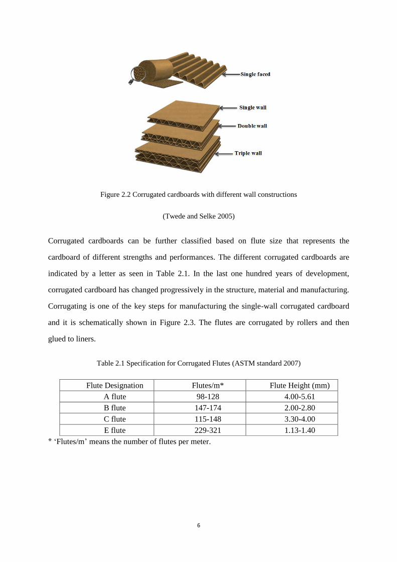
Figure 2.2 Corrugated cardboards with different wall constructions
(Twede and Selke 2005)
Corrugated cardboards can be further classified based on flute size that represents the
cardboard of different strengths and performances. The different corrugated cardboards are
indicated by a letter as seen in Table 2.1. In the last one hundred years of development,
corrugated cardboard has changed progressively in the structure, material and manufacturing.
Corrugating is one of the key steps for manufacturing the single-wall corrugated cardboard
and it is schematically shown in Figure 2.3. The flutes are corrugated by rollers and then
glued to liners.
Table 2.1 Specification for Corrugated Flutes (ASTM standard 2007)
Flute Designation Flutes/m* Flute Height (mm)
A flute 98-128 4.00-5.61
B flute 147-174 2.00-2.80
C flute 115-148 3.30-4.00
E flute 229-321 1.13-1.40
* ‘Flutes/m’ means the number of flutes per meter.

7
Figure 2.3 The corrugating procedure of a single wall corrugated board. (Allansson and Svärd 2001)
The manufacturing process makes fibers of the cardboards mainly oriented in the direction of
the machine, which lead to the anisotropy of the cardboards (Nordstrand 2003). Cardboards
are usually treated as orthotropic with three principal directions that are Machine Direction
(MD), Cross Direction (CD) and through-thickness direction (ZD), as shown in Figure 2.4.
Figure 2.4 Three principal directions of the orthotropic cardboard (Nordstrand 2003)
The mechanical behaviour of corrugated cardboards can be further divided into the in-plane
(x-y plane) and out-of-plane (z direction) behaviour. The in-plane and out-of-plane
behaviours can be characterized by stress and strain, as shown in Table 2.2. Note that σ
means stress while ε means strain, and x, y and z represent the three principal directions,
respectively.
8
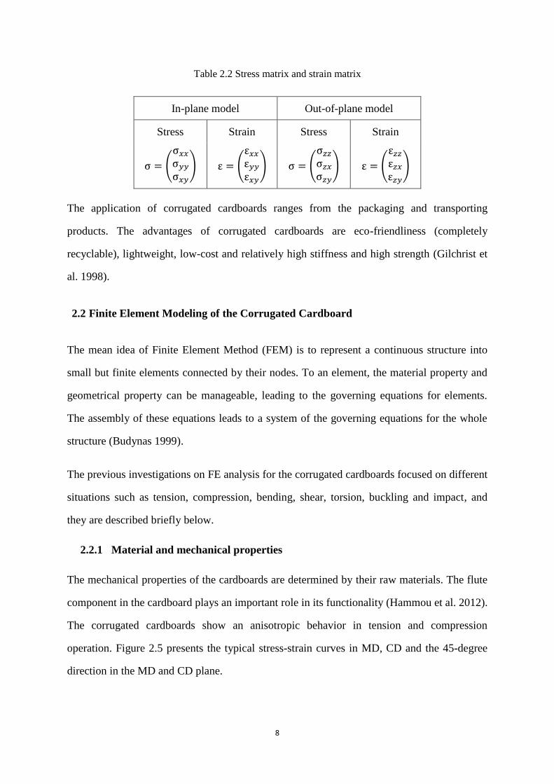
Table 2.2 Stress matrix and strain matrix
In-plane model Out-of-plane model
Stress Strain Stress Strain
σ = (
σ𝑥𝑥
σ𝑦𝑦
σ𝑥𝑦
) ε = (
ε𝑥𝑥
ε𝑦𝑦
ε𝑥𝑦
) σ = (
σ𝑧𝑧
σ𝑧𝑥
σ𝑧𝑦
) ε = (
ε𝑧𝑧
ε𝑧𝑥
ε𝑧𝑦
)
The application of corrugated cardboards ranges from the packaging and transporting
products. The advantages of corrugated cardboards are eco-friendliness (completely
recyclable), lightweight, low-cost and relatively high stiffness and high strength (Gilchrist et
al. 1998).
2.2 Finite Element Modeling of the Corrugated Cardboard
The mean idea of Finite Element Method (FEM) is to represent a continuous structure into
small but finite elements connected by their nodes. To an element, the material property and
geometrical property can be manageable, leading to the governing equations for elements.
The assembly of these equations leads to a system of the governing equations for the whole
structure (Budynas 1999).
The previous investigations on FE analysis for the corrugated cardboards focused on different
situations such as tension, compression, bending, shear, torsion, buckling and impact, and
they are described briefly below.
2.2.1 Material and mechanical properties
The mechanical properties of the cardboards are determined by their raw materials. The flute
component in the cardboard plays an important role in its functionality (Hammou et al. 2012).
The corrugated cardboards show an anisotropic behavior in tension and compression
operation. Figure 2.5 presents the typical stress-strain curves in MD, CD and the 45-degree
direction in the MD and CD plane.

9
Figure 2.5 Typical strain-stress curves of corrugated cardboards under tensile test (Hammou et al. 2012)
Because the fibres in the raw material of the cardboards tend to the MD during the
manufacturing process, the strength in this direction becomes quite larger than those in the
other directions. The other two principal directions are CD and ZD. The corrugated
cardboards are usually regarded as orthotropic in their constitutive relation.
In the previous study, some of the material parameters of corrugated cardboards were
measured successfully but many others were calculated by some empirical formula. Uniaxial
tension, compression and shear tests were usually applied to estimate the elastic modulus and
the hardening law of the cardboards.
Baum et al. (1981) established a set of empirical formula for calculating the Poisson ratios
and the in-plane shear modulus. Quite a number of papers applied Baum’s formula in their
models. In Baum’s formula, the in-plane shear modulus is a function of in-plane young’s
moduli, and two out-of-plane shear moduli are proportional to the corresponding in-plane
young’s modulus, respectively.
In two recent works of Huang (2013) and Thakkar et al. (2008), the most commonly used
method to determine the material parameters are shown in Table 2.3.

10
Table 2.3 The most commonly used determination method of material parameters in literature
Notes: (1)
Also used in the literatures (Mann et al. 1979; Baum et al. 1981; Nordstrand and Carlssonb 1997;
Stenberg 2003; Aboura et al. 2004; Hammou et al. 2012)
(2) DIC: Digital Image Correlation (Thakkar et al. 2008)
(3) Also used in the literature (Nordstrand 1995)
Among the sixteen parameters, only five of them were determined by a direct measurement.
The difficulty to get these constitutive parameters is seen as a bottleneck to improve the
accuracy of modeling of the cardboards.
In the earlier FE analysis for corrugated cardboards, researchers usually employed the linear
elastic model to model the behavior. Patel et al. (1997) created the nonlinear finite element
models by following the viscoelastic constitutive law. Gilchrist et al. (1998) developed a
plasticity nonlinear finite model to predict the bending and twisting behaviors. Besides the
Parameters Meaning Determination method
𝐄𝒙 elastic modulus in x-direction Tensile test
𝐄𝒚 elastic modulus in y-direction Tensile test
𝐄𝒛, elastic modulus in z-direction Empirical formula (=Ex 200⁄ ) (1)
𝝂𝒙𝒚, Poisson ratio in xy plane DIC (2)
𝝂𝒚𝒛, Poisson ratio in yz plane Assumed as 0.01(3)
𝝂𝒙𝒛, Poisson ratio in xz plane Assumed as 0.01(3)
𝑮𝒙𝒚 Shear modulus in xy plane Empirical formula (=0.387√E𝑥E𝑦)(1)
𝑮𝒚𝒛 Shear modulus in yz plane Empirical formula (=Ey 35⁄ ) (1)
𝑮𝒙𝒛 Shear modulus in xz plane Empirical formula (=Ex 55⁄ ) (1)
𝑬𝒕 Tangent modulus after the yield point Tensile test
𝑹𝒙𝒙 yield stress ratio in x-direction Assumed as 1
𝑹𝒚𝒚 yield stress ratio in y-direction Tensile test
𝑹𝒛𝒛 yield stress ratio in z-direction Estimate from a typical range
𝑹𝒙𝒚 yield stress ratio in 45º xy- plane Estimate from a typical range
𝑹𝒚𝒛 yield stress ratio in 45º yz- plane Estimate from a typical range
𝑹𝒙𝒛 yield stress ratio in 45º xz- plane Estimate from a typical range

11
material nonlinearity, there is nonlinearity caused from the non-linear geometry and change
in the contact between components such as flute and liner.
2.2.2 Element
Beam element and shell element were the two most commonly used elements in the previous
FE study for corrugated cardboards. Lu et al. (2001) and Krusper et al. (2008) adopted the
beam element in their models. Lu et al. (2001) exhibited an undulating behaviour in the
stress-stain curve. The model of Krusper et al. (2008) showed a smooth stress-strain curve
due to the lack of nonlinear material setting, based on the author’s comments. Djilali
Hammou et al. (2012) used 2D shell elements to simulate both liners and the flute of the
corrugated cardboard box for impact test. Haj-Ali et al. (2009) simulated the cardboard by
using 3D quadratic shell finite element while Talbi et al. (2009) implemented their model into
a 2D shell element in the same year. Talbi et al. (2009) also compared the 2D model with 3D
model and concluded that due to the discontinuous structure of the flute along MD
(x-direction), the flute’s contribution to resisting compression/tension and bending in MD can
be ignored and 2D theories may have sufficient accuracy; however, for certain loading
conditions such as transverse shear and torsion, the 3D structure has to be considered.
2.2.3 Geometry
Carlsson et al. (2001) investigated the effect of different shapes of flute on the in-plane
extensional stiffness, shear stiffness, bending stiffness and twisting stiffness. The shapes of
flutes were studied included circular profile, sinusoidal profile, trapezoidal profile and
triangular profile (Figure 2.6). The stiffness of cardboards with various geometry data, such
as height of the cardboard and the length of flute, were also compared.

12
Figure 2.6 Different flute profiles in FE models (Carlsson et al. 2001)
Biancolini et al. (2003) observed that the actual flute shape is not as same as the sine shape
applied in many previous FE models and obtained the cross-section contour of the actual flute
by photographic magnification. Biancolini (2005) further studied the stiffness feature of
saw-tooth profile, sinusoidal profile and actual profile of corrugated cardboard (Figure 2.7).
Figure 2.7 (a) Actual profile; (b) Sine profile and (c) Saw-tooth profile in FE model (Biancolini 2005)
2.2.4 Contact Problem
Adhesive: The adhesive glues flute and liners in real world and the gluing behavior may be
modelled in the FE models. The assumption of fully bond was used most frequently in the
previous models (Aboura et al., 2004), and this assumption further led to the model that the
flute and liners shared the same nodes. Haj-Ali et al. (2009) and Jiménez-Caballero et al.
(2009) utilized an isotropic and 3D solid (or called brick element) adhesive model. Pommier
et al. (1991) simulated the adhesive by applying multi point constraints (MPC’s) and the
short shell elements, respectively. The investigations implied that the models of the adhesive

13
are an important factor to the stress-strain behaviour, especially the ultimate values of stress
and strain (Haj-Ali et al. 2009).
Friction model: Thakkar et al. (2008), Dayyani et al. (2011) and Hammou et al. (2012)
studied the friction model between flute and liners. However, to the author’s best knowledge,
there is little published work which studied the impact of the friction model to the
performance of the whole FE model of the corrugated cardboard. In the occasion of modeling
of the compression testing process, the friction between the compression head and liners is
usually ignored (in particular the friction is large enough to hold together the liner and
compression head); see the work of Krusper et al. et al. (2008) and Huang (2013). However,
the work by Rajesh et al. (2013) observed that for a ring metal specimen rather than
cardboard that the friction at the interface significantly affects its deformation and the
stress-strain result under the compression test.
2.2.5 Impact and Vibration Problem
The shock or impact damage is inevitable during storage and transportation for the corrugated
cardboards packages. Nguyen et al. (2005) simulated the low velocity impact of
honeycomb-structure panels. By applying a software tool called Sandmesh tool for explicit
impact analysis, the geometry of the indentation was predicted successfully. Sek (2009) built
a FE model for multilayer corrugated cardboards structure impacted by a freefalling mass.
The collapsible structure such as the corrugated cardboards exhibits the dissipative effect
when subjected to impact and this effect can attenuate shock.
Djilali Hammou et al. (2012) created a homogenization FE model of free drop tests aim to
deal with the impact problem of corrugated cardboards packages and claimed that the
corrugated cardboards box is able to absorb shock energy. Huang (2013) confirmed the
function of absorbing the dynamic energy of the corrugated cardboards and also measured the
damping of cardboards, designed the cardboard-based isolator, and validated the design by
experiments.

14
2.2.6 Compression Problem
To the best knowledge of the author, there are only three published papers, Huang (2013);
Krusper et al. (2008); Lu et al. (2001) explicitly explained the FE model for the corrugated
cardboards under the through- thickness- direction compression.
The FE model of Lu et al. (2001) applied the 2-D beam elements and surface contact element
and behaviors by following the bi-liner constitutive law. The stress-strain curves for the
specimen of two commonly used compression tests FCT (Flat Crush Test) and CMT
(Concorra Medium Test) were found with FEM (Figure 2.8) (Lu et al. 2001). FCT specimen
consists of the complete unit of the cardboard structure with both liner and flute while the
CMT specimen has only the flute and an adhesive tape but without liners. The contact
between the flute and the liners was modeled as frictionless in the simulation of FCT and as
sticky in the case of CMT. The uniform compressive displacement in the through-thickness
direction was applied on the upper liner of FCT model and on an imaginary rigid line where
the upper liner was placed. The conclusion made was that the properties of the flute mainly
drive the mechanical behavior of the corrugated cardboards subjected to a through-thickness
compressive force (Lu et al. 2001).

15
Figure 2.8 One-unit corrugated cardboards specimens for (a) FCT and (b) CMT (Lu, Chen, & Zhu,
2001)
Both of the FE models of FCT and CMT exhibited undulating curves for the stress versus
strain behavior. Two different kinds of boundary conditions for the FE model were analysed
in their investigation: the so-called ‘periodic’ boundary conditions and ‘free-edge’ boundary
conditions. The former conditions mean that all of the DOFs of upper liner, lower liner and
the flute were constrained except the vertical translations of the upper liner and the flute. The
latter conditions set all of the DOFs of the liners and the flute as free but the vertical
translation of the lower liner was restrained. It was reported that when the ratio of liner’s
thickness to flute’s thickness is larger than 0.5, which is in the way of most commercially
available corrugated cardboards present, the ‘free-edge’ boundary conditions exhibit a more
accurate prediction than the ‘periodic’ one on the stress-strain behavior. Lu et al. (2001) also
studied how the geometrical and material parameters affect the FE model’s performance and
the geometrical imperfection of the flute. At last, the FE results were compared with the
experimental results. The comparison is shown in Figure 2.9.
16
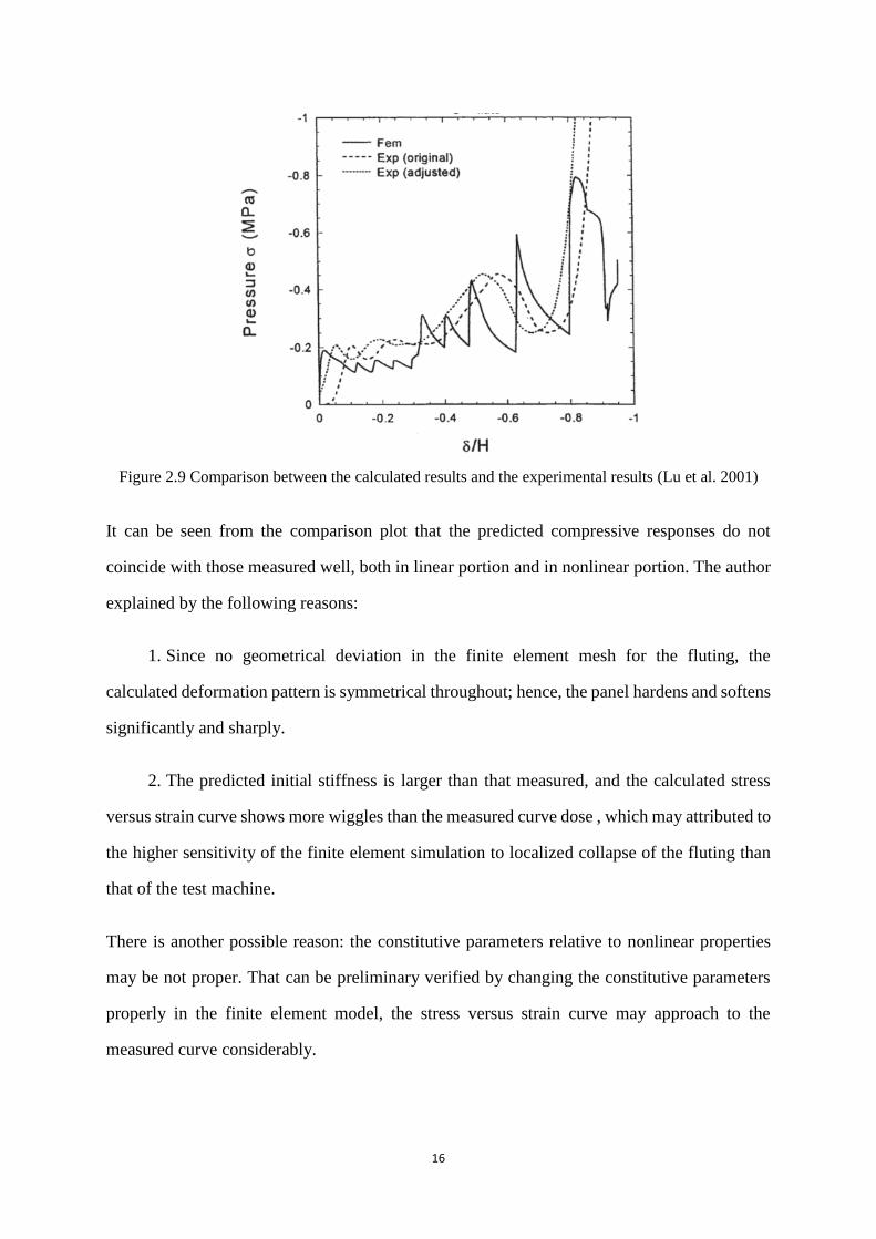
Figure 2.9 Comparison between the calculated results and the experimental results (Lu et al. 2001)
It can be seen from the comparison plot that the predicted compressive responses do not
coincide with those measured well, both in linear portion and in nonlinear portion. The author
explained by the following reasons:
1. Since no geometrical deviation in the finite element mesh for the fluting, the
calculated deformation pattern is symmetrical throughout; hence, the panel hardens and softens
significantly and sharply.
2. The predicted initial stiffness is larger than that measured, and the calculated stress
versus strain curve shows more wiggles than the measured curve dose , which may attributed to
the higher sensitivity of the finite element simulation to localized collapse of the fluting than
that of the test machine.
There is another possible reason: the constitutive parameters relative to nonlinear properties
may be not proper. That can be preliminary verified by changing the constitutive parameters
properly in the finite element model, the stress versus strain curve may approach to the
measured curve considerably.

17
Krusper et al. (2008) developed an analytical model for calculation the nonlinear deformation
of the fluting under vertical compressive loads and compared the analytical model with a
finite element model and with experimental results. The comparison is shown in Figure 2.10
where the FE results agree well with the analytical results. In particular, the linear part in the
experimental curve agrees well with those in both analytical and FE model curve. However,
there is a big difference in the nonlinear part. This is because the nonlinear material
properties of the flute and the liner in the FE model were not considered.
Figure 2.10 Comparison between solutions obtained by analytic model, FE model and experiment
(Krusper et al., 2008)
Huang (2013) refined the finite element model of Lu et al. (2001) and Krusper et al. (2008)
by changing the element type from beam element to the shell element and by considering the
nonlinear orthotropic material property. The constitutive model in Huang’s work consisted of
two parts: the elastic portion and the plastic portion. The elastic portion followed the Hook’s
Law, while the plastic part was governed by a quadratic Hill yield criterion. In these
constitutive models, there were sixteen unknown parameters in total, but only four of them
were experimentally measured, while the other value of parameters were derived by the
empirical formula or from an empirical range (see details in Table 2.3). The comparison
between the FEM results and the experimental results (60.8 mm×38 mm) is shown in Figure
2.11. It can be found from the figure that the FEM result dose not correlate well with the

18
experimental result in the nonlinear portion (after reaching the peak at the displacement of
about 0.75 mm). This situation is because the plastic model property was not correct.
Figure 2.11 Comparison of the experimental results and FEM results (Huang 2013)
Overall, Lu et al. (2001), Krusper et al. (2008) and Huang (2013) performed a finite element
analysis for the cardboard by considering some non-linear behavior of the cardboard.
However, there is a common disadvantage in their models: the peak load and the subsequent
nonlinear response cannot be predicted accurately. This is because the nonlinear material
property of the cardboard in their models is not accurate.
2.3 Vibration Isolation
Vibration isolations are divided into two categories: passive isolation and active isolation.
Passive vibration isolation refers to vibration isolation methods of using the materials such as
rubber pads, mechanical springs or sheets of flexible materials. Active vibration isolation
refers to employing the electric power, sensors, actuators, and control systems to adjust the
isolation behavior in a real-time fashion (De Silva 2006). The mean advantage of the passive
system over the active system is that the passive system is less expensive and easy to
construct. The corrugated cardboard, which is used as vibration isolation in this study, is
considered as a passive isolation system.
19
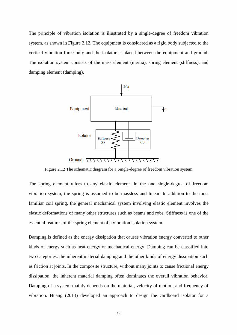
The principle of vibration isolation is illustrated by a single-degree of freedom vibration
system, as shown in Figure 2.12. The equipment is considered as a rigid body subjected to the
vertical vibration force only and the isolator is placed between the equipment and ground.
The isolation system consists of the mass element (inertia), spring element (stiffness), and
damping element (damping).
Figure 2.12 The schematic diagram for a Single-degree of freedom vibration system
The spring element refers to any elastic element. In the one single-degree of freedom
vibration system, the spring is assumed to be massless and linear. In addition to the most
familiar coil spring, the general mechanical system involving elastic element involves the
elastic deformations of many other structures such as beams and robs. Stiffness is one of the
essential features of the spring element of a vibration isolation system.
Damping is defined as the energy dissipation that causes vibration energy converted to other
kinds of energy such as heat energy or mechanical energy. Damping can be classified into
two categories: the inherent material damping and the other kinds of energy dissipation such
as friction at joints. In the composite structure, without many joints to cause frictional energy
dissipation, the inherent material damping often dominates the overall vibration behavior.
Damping of a system mainly depends on the material, velocity of motion, and frequency of
vibration. Huang (2013) developed an approach to design the cardboard isolator for a

20
vibratory machine. However, the damping was ignored in his approach, which may need
more deliberation and re-thinking.
2.4 Conclusion
This chapter introduced the background and reviewed the literature about corrugated
cardboards with a focus on its application of vibration isolation and the finite element
modeling. The discussion may have given a sufficient argument that the accuracy of the FE
model may be improved by giving further attention to the determination of the material
parameters in the constitutive relation. Further, more accurately modeling the contact
between the liner and flute in the cardboards may also be a factor to improve the accuracy of
the model. Last, the damping behavior may need to be studied in the context of the vibration
isolation system made of the cardboards.

21
CHAPTER 3 DETERMINATION OF CONSTITUTIVE PARAMETERS
3.1 FE Model
The FE model of the corrugated cardboards in this paper was built upon the model of Huang
(2013). In the following, this model is explained.
3.1.1 Element
Shell elements were used to analyze the thin structures. In this case, the shell 181 was used
due to its better performance to deal with the nonlinearity. The shell 181 element is a
first-order quadrilateral element. It is defined by four nodes: I, J, K, L with three translational
and three rotational degrees of freedom at each node, as seen in Figure 3.1. Figure 3.1 also
denotes the geometry, node locations, and the element coordinate system for this element.
Note x and y are in the plane of the element. The default orientation of the element coordinate
system is θ = 0 (Figure 3.1).
Figure 3.1 The geometry of the shell 181 element(ANSYS Inc. 2004)
22
The shell 181 element obeys the Mindlin theory which has basic assumptions (Imaoka 2000;
ANSYS Inc. 2004). (1) The straight line normal to the mid-surface before deformation
remains straight after loading, but not necessarily normal to the mid-surface. (2) The through-
thickness stress is negligible. (3) Each set of integration points thru a layer is assumed to have
the same element (material) orientation. (4) The change in thickness is due to the “stretching”
of the shell only. It is noted that the major advantage of shell 181 is that it is capable of large
deformation and it supports most material nonlinearities.
3.1.2 Nonlinearity
In the finite element analysis process, the nonlinear problems fall into the following three
categories, and all of them are considered in this study. The three kinds of nonlinear
behaviors or properties of the material are (1) Geometrical nonlinearity (2) material
nonlinearity, and (3) boundary condition nonlinearity.
Geometry nonlinearity is caused by large deformation of the element such that the
relationship between load and deformation is not linear. For instance, the so-called continuity
equation is not linear; in particular the relationship between the strain and displacement and
its derivative is not linear. Material nonlinearity refers to the material constitutive relation in
particular the stress and strain relationship is nonlinear. Boundary condition nonlinearity
refers to the relationship between force and displacement and its derivative on the boundary
is nonlinear. A typical problem of boundary nonlinearity comes from the contact problem.
3.1.3 Contact problems
In this model, the liner and the core share the same node and apply to the surface-to-surface
contact condition in their connecting area. In the surface-to-surface contact condition, it is
important to identify contact surface and target surface since the contact algorithm set rules
that the nodes on the target surface cannot penetrate into the contact surface. There are
several intuitive but rough criterions commonly used to select the contact surface and target
surface, such as the convex, softer, smaller; otherwise fine meshed surfaces are usually
selected as the contact surface while the concave, flat, coarse meshed, stiffer or lager surfaces

23
are usually considered as the target surface. In this study, the contact surface is assigned to
the surface of the flute and the target surface is set to the surface of the liner.
3.2 Constitutive law
As mentioned above, Huang’s constitutive model consists of the elastic portion following the
Hook’s Law and the plastic portion governed by Hill yield criterion and isotropic hardening
law. The elastic orthotropic constitutive model is assumed to be one as follows (Allansson
and Svärd 2001):
x
10 0 0
10 0 0
10 0 0
10 0 0 0 0
10 0 0 0 0
10 0 0 0 0
yx zx
x y z
xy zy
x y z x
y
yyzxzz
zx y zx
xy
y
xzxyz
yz
xz
yz
E E E
E E E
E E E
G
G
G
(3.1)
where
x , y , z : strain in x, y, z direction,
γxy, γxz, γyz : strain in xy, xz, yz plane,
Ex, Ey, Ez : Young’s modulus in x, y, z direction,
νxy, νxz, νyz : Poisson’s ratio in xy, xz, yz plane, and
Gxy, Gxz, Gyz : shear modulus in xy, xz, yz plane.
The yield criterion is given by (ANSYS Inc. 2004)
0)(0 pTMf
(3.2)

24
where
0 : yield stress in the x direction,
p : equivalent plastic strain,
: yield stress matrix, and
M : plastic compliance matrix.
The plastic compliance matrix M (ANSYS Inc. 2004) can be written as:
0 0 0
0 0 0
0 0 0
0 0 0 2 0 0
0 0 0 0 2 0
0 0 0 0 2
0
G H H G
H F H F
G F F G
K
I
M
J
(3.3)
F, G, H, I, J and K are material constants that can be determined experimentally. According
to ANSYS (2004), these are defined as:
)111
(2
1222
xxzzyy RRRF
(3.4)
)111
(2
1222
yyxxzz RRRG
(3.5)
)111
(2
1222
zzyyxx RRRH
(3.6)
2
3 1( )
2 yz
IR
(3.7)
2
3 1( )
2 xz
JR
(3.8)

25
2
3 1( )
2 xy
KR
(3.9)
In the above, the ratios of yield stresses yzxyzzyyxx RRRRR ,,,, and xzR (ANSYS Inc. 2004) are
further calculated by
0
y
xxxxR
(3.10)
0
y
yy
yyR
(3.11)
0
y
zzzzR
(3.12)
0
3
y
xy
xyR
(3.13)
0
3
y
yz
yzR
(3.14)
0
3
y
xzxzR
(3.15)
where y
ij is the yield stress in the x, y, z, xy, yz and xz directions, respectively. The six
yield stress ratios are direct input items in the FE model when the reference stress 0 is
defined – see Equation (3.10) to (3.15).
The hardening rule determines when the material will yield again if the loading is continued
or reversed. There are two basic hardening rules to prescribe the evolution of the yield
surface compared to the Initial Yield surface: Kinematic hardening and Isotropic hardening.
Isotropic hardening means that the yield surface remains constant in size and translates in the
direction of yielding. The Isotropic hardening implies that the yield surface increases in size
uniformly in all directions with the plastic flow. For a solid that follows the isotropic
26
hardening rule, if it is unloaded after a plastic deformation, reloading it again will lead to its
yield stress to increase. The isotropic hardening rule is chosen to describe such plasticity.
Therefore, the plastic slope of the material after yield point (ANSYS Inc. 2004) is:
tx
txpl
EE
EEE
(3.16)
where
xE : Elastic modulus in x direction, and
tE : Tangent modulus after the yield point.
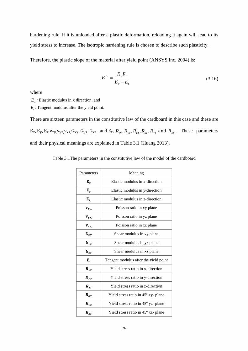
There are sixteen parameters in the constitutive law of the cardboard in this case and these are
Ex, Ey, Ez,νxy,νyz,νxz,Gxy, Gyz, Gxz and Et,yzxyzzyyxx RRRRR ,,,, and xzR . These parameters
and their physical meanings are explained in Table 3.1 (Huang 2013).
Table 3.1The parameters in the constitutive law of the model of the cardboard
Parameters Meaning
𝐄𝒙 Elastic modulus in x-direction
𝐄𝒚 Elastic modulus in y-direction
𝐄𝒛, Elastic modulus in z-direction
𝝂𝒙𝒚, Poisson ratio in xy plane
𝝂𝒚𝒛, Poisson ratio in yz plane
𝝂𝒙𝒛, Poisson ratio in xz plane
𝑮𝒙𝒚 Shear modulus in xy plane
𝑮𝒚𝒛 Shear modulus in yz plane
𝑮𝒙𝒛 Shear modulus in xz plane
𝑬𝒕 Tangent modulus after the yield point
𝑹𝒙𝒙 Yield stress ratio in x-direction
𝑹𝒚𝒚 Yield stress ratio in y-direction
𝑹𝒛𝒛 Yield stress ratio in z-direction
𝑹𝒙𝒚 Yield stress ratio in 45º xy- plane
𝑹𝒚𝒛 Yield stress ratio in 45º yz- plane
𝑹𝒙𝒛 Yield stress ratio in 45º xz- plane

27
The necessity to conduct the identification for each parameter in the constitutive function of
the cardboard-model will be analyzed and the selected parameters will be identified through
the numerical-experimental identification procedure.
3.3 Experimental Setup
To determine the aforementioned constitutive parameters, a system for the measurement of
the behaviour of corrugated cardboards needs to be set up. The behavior considered in this
study was the stiffness in the vertical direction or ZD (Figure 2.4). In this case, the setup used
for building Huang’s FE model was used. Further, the commercially available corrugated
cardboard from the Company denoted as C was used in the compression (along ZD)
experiment. The geometry for the type-C cardboard is shown in Figure 3.2 and the
geometrical parameters of the cardboard are listed in Table 3.2.
Figure 3.2 Geometry of the type-C cardboard
Table 3.2 Geometry of the corrugated cardboard specimen (mm)
Flute
Type Length Width Height
Flute length
(λ)
Thickness
of liner (𝑡𝑙)
Thickness
of flute (𝑡𝑓)
C 30.4 38 3.6 7.6 0.28 0.28
The through-thickness compressive test for the corrugated cardboards followed the method in
the thesis of Huang (2013). The force verses displacement curve was recorded through the
compressive test. Figure 3.3 depicts a typical force-displacement curve drawn from the
compressive test. Due to the so-called ‘washboard effect’ (i.e., the non-flatness of the liner),
the initial stage of a force-displacement curve of the experimental result was neglected.

28
Figure 3.3 The typical force-displacement curve in compressive experiment
3.4 Parameter identification procedure
The general idea of application of the system identification technique to the determination of
the system parameter was to determine the parameter in a system or model based on the
fitting of the behavior of the system predicted and measured on a particular instance. In our
case, the parameter is the constitutive parameter of the cardboard, and the behavior is the
stiffness along ZD, and the prediction method is the finite element method (as described in
the above). In applying this technique, the parameters in a model are thus taken as a variable
and the problem model is an optimization problem.
The commercial software ANSYS® with the built-in OPT processor was adopted as an
optimization tool. ANSYS allows the user to choose the optimization algorithm and to define
the objective function, design variables and constraints (ANSYS Inc. 2005). Three steps were
followed to accomplish this task: (1) Define design variables (DVs), (2) Define State
Variables (also called constraint, SVs), and (3) Define objective variables (OVs).
3.4.1 Design variables (DVs)
Design variables are those 16 constitutive parameters (see Table 3.1). Because the liner and
flute have the same constitutive equation but different constitutive parameters, there are in
total 32 parameters. To an optimization problem, 32 parameters may create some
Washboard effect stage

29
computational overhead. It is certainly helpful to reduce the number of variables in
optimization. Therefore, an attempt to discard some parameters was taken. A general
principle to get rid of some parameters is to examine the significance of their effect of the
parameters on the response of the FEM model, that is, force-displacement curve in this case.
A coefficient R was introduced to represent the sensitivity of the parameters to the
force-displacement curve, which is the ratio of the percent change of the ultimate force in the
force-displacement curve and the change in the material parameters.
R =∆ ultimate force %
∆material parameter %
(3.17)
Another principle is to examine the effects of the parameters in terms of their physical
meanings, and for this purpose, the 32 parameters are divided into five groups that have the
physical meaning.
a. Young’s modulus
Following the assumption in the shell 181 element, the stress through-thickness is considered
as zero (ANSYS Inc. 2005). This further implies that any change in the thickness of the
element is due to the “stretching” of the shell only and the thickness of the element will not
change when the element is compressed along the thickness direction. Thus, E𝑧 ≡ 0, where
E𝑧 is the out-of-plane young’s modulus (see Figure 3.1).
E𝑧will not affect the result of the finite element calculation for the shell element. This was
verified by the calculation with the FEM for different E𝑧 (in particular by randomly
changing E𝑧 of either flute or liner material or both). The calculation showed no significant
change against a reference force-displacement curve. In fact, this can also be explained by
Mindlin’s theory of plates that there is no through-thickness stress in plates; therefore, the
young’s modulus in z-direction would be considered as zero.
For the in-plane Young’s modulus (i.e., Exl , Exf , Eyl and Eyf ), these were changed
incrementally (see Table 3.3) and then calculate the stiffness along the z-direction for the

30
different increments of them. It is noted that in the term of Exl, Exf, Eyl and Eyf, x and y refer
to the two axes as denoted in Figure 3.1, and further, ‘l’ means liner and ‘f’ means the flute.
For example, Exl means the elastic modulus in the x-direction for the liner. In total, nine models
were created by changing one Young’s modulus each time by using model 1 as the reference
model. Unless otherwise stated in this chapter, model 1, also called the reference model, is
the same as that in Huang’s thesis (Huang 2013).
After calculations, the force-displacement curves of the nine models are obtained. The
ultimate forces of the nine force-displacement curves are listed in Table 3.3.
Table 3.3 Sensitivity of In-plane Young’s moduli in comparison calculations
The calculated results showed that the in-plain Young’s moduli of liner Exl (model 1, 2 and
3) and Eyl (model 1, 6 and 7) had no influence on the stress-strain response with a
sensitivity of zero. The calculated result showed a strong independence on Eyf (model 1, 8
and 9) by an average sensitivity of 0.08 for increase and decrease. Exf (model 1, 4 and 5)
affects the stress-strain curve more strongly with an average sensitivity of 2.95. In conclusion,
the six design parameters of Young’s moduli reduce to only one key parameter Exf which
has a significant influence.
Model
number
1
(Reference) 2 3 4 5 6 7 8 9
Changed
parameter —─— Exl Exl Exf Exf Eyl Eyl Eyf Eyf
Changed value
(Gpa)
(Reference value)
—─— 2.5
(3.2)
5.0
(3.2)
2.5
(3.2)
5.0
(3.2)
1
(2)
3
(2)
1
(2)
3
(2)
Ultimate
force (N) 197.69
197.69
197.69
195.27
202.09
197.69
197.69
197.70
197.86
Sensitivity R —─— 0 0 3.46 2.44 0 0 -0.01 0.17

31
b. Poisson’s ratios
Poisson’s ratios are classified into two categories based on the directions. These are in-plane
Poisson’s ratio 𝜈𝑥𝑦 and the out-of-plane Poisson’s ratios 𝜈𝑦𝑧 and 𝜈𝑥𝑧 . The in-plane
Poisson’s ratio is measured by tensile test as the form of a ratio of lateral to longitudinal
strain. The out-of-plane Poisson’s ratios are generally neglected in literatures due to its
relatively small effect to the compression response. In the papers of Thakkar et al. (2008) and
Huang (2013), 𝜈𝑦𝑧,𝜈𝑥𝑧 are assumed to be 0.01. To verify whether the Poisson’s ratios have
any effect on the compression response, ten calculations were taken. First four calculations
changed 𝜈𝑥𝑦 from 0.3 to 0.45 with an interval of 0.05 and six other one assigned 0.01, 0.05
and 0.1 to 𝜈𝑦𝑧 and 𝜈𝑥𝑧 separately. Only one parameter was changed in each calculation,
while all the rest parameters stayed the same as these were in the reference model. The
force-displacement results show that there is barely change in these calculations, which imply
that change of the Poisson’s ratios 𝜈𝑥𝑦, 𝜈𝑦𝑧 𝑎𝑛𝑑 𝜈𝑥𝑧 has negligible influence on the
calculated result in this FE model. Note that the results in this section are applicable to
Poisson’s ratios of both the flute and liner.
c. Shear modulus
The shear moduli were often calculated with empirical formulas (Mann et al. 1979; Baum et
al. 1981) in literature. To examine whether the shear moduli affect the response of the
compression model, the calculations were taken. The values of the changed parameters and
their reference values are listed in Table 3.4. Model 1 is the reference model. Models 2-7
reduced each shear modulus by half while all the rest parameters keep the same as these are
in the reference model. The force-displacement characteristics under these conditions are
plotted in Figure 3.4.

32
Table 3.4 Sensitivity of Shear moduli in comparison calculations
Model
Number
1
(Reference) 2 3 4 5 6 7
Changed
parameter —─— Gxyl* Gxyf* Gxzl Gxzf Gyzl Gyzf
Changed value
(GPa)
(Reference value)
—─— 0.5
(1)
0.5
(1)
0.057
(0.0285)
0.005
(0.0025)
0.058
(0.029)
0.05
(0.025)
Ultimate
force (N) 197.69
197.69
197.69
197.69
122.60
197.69
197.71
Sensitivity R —─— 0 0 0 -3e4 0 -0.8
* Gxyl means the shear modulus of liner in xy-plane; Gxyf is the shear modulus of flute in xy-plane, etc.
Figure 3.4 The force-displacement curves with different Shear moduli
The force-displacement curves of the model 1-7 shows that none of the shear moduli affects
the result of the calculation significantly except the model 5 (related to Gxzf). It can be found
in Table 3.4 that the response of the model 5 strongly depends on Gxzf with the sensitivity of
33
-3e4. Figure 3.4 shows that Gxzf has a great influence on both the elastic portion and the
plastic portion in the force-displacement curve. It is noted that the strong influence of the
out-of-plane shear moduli on the frequency property rather than the stiffness property of
paperboards was verified in the previous study by Schwingshackl et al. (2006). The analysis
here seems to be in consistence with their result.
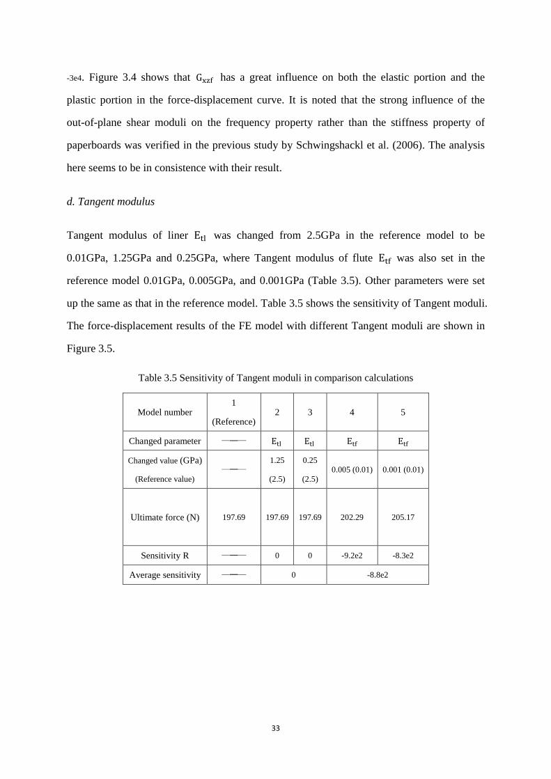
d. Tangent modulus
Tangent modulus of liner Etl was changed from 2.5GPa in the reference model to be
0.01GPa, 1.25GPa and 0.25GPa, where Tangent modulus of flute Etf was also set in the
reference model 0.01GPa, 0.005GPa, and 0.001GPa (Table 3.5). Other parameters were set
up the same as that in the reference model. Table 3.5 shows the sensitivity of Tangent moduli.
The force-displacement results of the FE model with different Tangent moduli are shown in
Figure 3.5.
Table 3.5 Sensitivity of Tangent moduli in comparison calculations
Model number 1
(Reference) 2 3 4 5
Changed parameter —─— Etl Etl Etf Etf
Changed value (GPa)
(Reference value) —─—
1.25
(2.5)
0.25
(2.5) 0.005 (0.01) 0.001 (0.01)
Ultimate force (N) 197.69
197.69
197.69
202.29
205.17
Sensitivity R —─— 0 0 -9.2e2 -8.3e2
Average sensitivity —─— 0 -8.8e2

34
Figure 3.5 The force-displacement curves with different tangent moduli
From Table 3.5 and Figure 3.5, it can be seen that Etl has no influence on the response and
with the model 1, 2 and 3, while Etf has more significant influence on the response curve
with the model 1, 4 and 5. Note that the influence only presents in the plastic portion.
Moreover, Etf have a positive correlation with the force from the yield point to the point A
and a negative correlation after the point A (Figure 3.5). The average of the sensitivity to the
ultimate force is -8.8e2 (Table 3.5).
e. Yield stress ratios
There are six parameters characterizing the Hill yield criterion in the FE model, which are
yield stress ratios Rxx, Ryy, Rzz, 𝑅𝑥𝑦, 𝑅𝑦𝑧 𝑎𝑛𝑑 𝑅𝑥𝑧 (ANSYS Inc. 2004) (see Chapter 1 for
details). The analysis showed that only the yield stress ratio in the x-direction Rxx has a
significant influence on the force-displacement curve while the other five ratios make no
difference and can thus be neglected. Table 3.4 lists the sensitivity of Rxx in the range of 0.5
to1. From this table, it can be seen that Rxx strongly affects the force-displacement curves
with the average sensitivity of 88.62. The response curves with a different Rxx are plotted in
Figure 3.6. It can be seen from the figure that Rxx strongly affects the plastic behavior of the
A
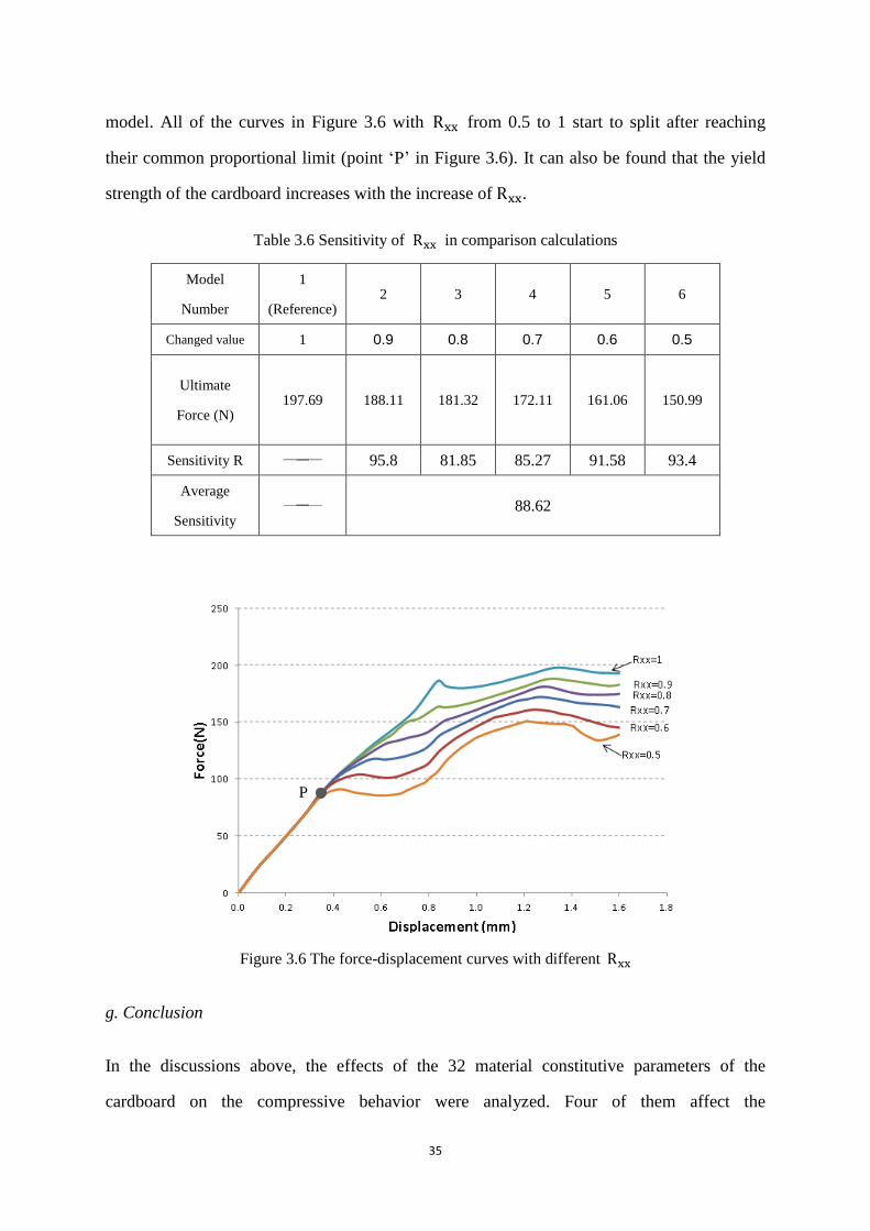
35
model. All of the curves in Figure 3.6 with Rxx from 0.5 to 1 start to split after reaching
their common proportional limit (point ‘P’ in Figure 3.6). It can also be found that the yield
strength of the cardboard increases with the increase of Rxx.
Table 3.6 Sensitivity of Rxx in comparison calculations
Model
Number
1
(Reference) 2 3 4 5 6
Changed value 1 0.9 0.8 0.7 0.6 0.5
Ultimate
Force (N) 197.69
188.11
181.32
172.11 161.06
150.99
Sensitivity R —─— 95.8 81.85 85.27 91.58 93.4
Average
Sensitivity —─— 88.62
Figure 3.6 The force-displacement curves with different Rxx
g. Conclusion
In the discussions above, the effects of the 32 material constitutive parameters of the
cardboard on the compressive behavior were analyzed. Four of them affect the
P
36
force-displacement curve more strongly than the other parameters. Thus, the total number of
independent parameters is reduced from 32 to 4 and the four parameters are: Exf, Etf, Gxzf
and Rxx. These parameters will be fine-tuned, and in other words, they were the variables in
the optimization model (notice: the parameter identification problem of the system was
represented as an optimization problem).
3.4.2 Constraint
The constraints of design variables (DVs) were made in Table 3.7 (Schwingshackl et al. 2006;
Thakkar et al. 2008; Huang 2013). In ANSYS, tolerance is the acceptable variation in the
DVs between loop computations to determine the convergence criterion. In this analysis, the
tolerance of DV is set as default that equals 0.01 times the current value.
Table 3.7 Constraint on the optimization variables
Design Variable Meaning Lower limit (GPa) Upper limit (GPa)
𝑬𝒙𝒇 elastic modulus in x-direction 0.5 6
𝑮𝒙𝒛𝒇 Shear modulus in xz plane 0.003 0.01
𝑬𝒕𝒇 Tangent modulus of core 0.001 0.05
𝑹𝒙𝒙 yield stress ratio in x-direction 0.9 1
3.4.3 Objective variables (OVs)
The objective variable is the variable in the optimization, which needs to be minimized. In
the problem the present work was concerned, the objective variable was the least-square
deviation between the calculated and measured force-displacement, that is:
OBJ= ε(Q) =1
𝑛∑ (
𝐹𝑠𝑖𝑚(𝑈𝑖,𝑄)−𝐹𝑒𝑥𝑝(𝑈𝑖)
𝐹𝑒𝑥𝑝(𝑈𝑖))2𝑛
𝑖=1 (3.18)
where n is the number of force-displacement points adopted in the calculated and measured
curve. 𝐹𝑠𝑖𝑚 means the calculated force and 𝐹𝑒𝑥𝑝 is the measured force; 𝑈𝑖 represents
the displacement of the 𝑖th point. Q is the design variable set.

37
3.4.4 Optimization method
In ANSYS, two optimization methods are available: the sub-problem approximation method
and the first order method. The sub-problem approximation method applies a zero-order
algorithm that only requires the values of the dependent variables rather than their derivatives,
which is generally capable of dealing with most of the engineering problems. The first order
method requires the information of first order derivative of the dependent variables, leading
to a higher accuracy but a higher computational cost. In this thesis, the sub-problem
approximation method was chosen. ANSYS offers a number of optimization tools such as
single-loop analysis, random, sweep, factorial and gradient tools as well. In this case, the
Sweep tool analyses each design variable (DV)’s sensitivity to the objective function in the
global design space. In this analysis, the sweep tool actually scans the design space, so it gets
the information of the objective function over the domain. By examining this information,
one can identify the one that is the smallest value of the objective function, which
corresponds to the optimal design variable. The sub-problem approximation method and
sweep tool are briefly introduced in the following.
Sub-problem approximation method
Consider that a general constrained problem is expressed as follows (ANSYS Inc. 2004):
where 𝑓(𝑥) is the objective function (the objective variable ‘f’), 𝑔𝑖(𝑥), ℎ𝑖(𝑥) 𝑎𝑛𝑑 𝑤𝑖(𝑥)
are constraint functions.
In the sub-problem approximation method, the objective variable and the constraint variables
are first replaced by (ANSYS Inc. 2004):
min f = f(x) (3.19)
gi(x) ≤ gimax (i = 1,2,3, … , m1) (3.20)
himin ≤ hi(x) (i = 1,2,3, … , m2) (3.21)
wimin ≤ wi(x) ≤ wimax (i = 1,2,3, … , m3) (3.22)

38
The constraints are converted to the unconstrained optimization problem by using a penalty
function. The penalty function satisfies: if independent variables (e.g.,𝑥, in this case) are
feasible, the penalty function is zero; otherwise it is greater than zero. In this case, X, G, H,
and W are defined as a penalty function for the design variable and constraint. As such, the
problem becomes (ANSYS Inc. 2004):
Minimize
where 𝑓0 is the reference objective function value used to achieve consistent unit. 𝑃𝑘 is a
response surface parameter. The subscript k is the number of the iterations during the
sub-problem optimization process. 𝑃𝑘 is increased in value as k increases, that is,
(𝑃1 > 𝑃2 > 𝑃3 𝑒𝑡𝑐.) in order to obtain accurate, converged results.
Convergence: when the convergence is reached, the sub-problem approximation iteration
stops. Convergence is assumed that if all the present design 𝑓(𝑗), the previous design 𝑓(𝑗−1)
and the best design set 𝑓(𝑏) are feasible design; and one of the following conditions is
satisfied (ANSYS Inc. 2004).
𝑓(𝑥) = 𝑓(𝑥) + 𝑒𝑟𝑟𝑜𝑟 (3.23)
�̂�(𝑥) = 𝑔(𝑥) + 𝑒𝑟𝑟𝑜𝑟 (3.24)
ℎ̂(𝑥) = ℎ(𝑥) + 𝑒𝑟𝑟𝑜𝑟 (3.25)
�̂�(𝑥) = 𝑤(𝑥) + 𝑒𝑟𝑟𝑜𝑟 (3.26)
F(�̅�, 𝑃𝑘) = 𝑓 + 𝑓0𝑃𝑘 (∑ 𝑋(𝑥𝑖) + ∑ 𝐺(�̂�𝑖) + ∑ 𝐻(ℎ̂𝑖)
𝑚2
𝑖=1
𝑚1
𝑖=1
𝑛
𝑖=1
+ ∑ 𝑊(�̂�𝑖)
𝑚3
𝑖=1
) (3.27)

39
where: 𝜏 is the objective function tolerance and 𝜌𝑖 is the design variable tolerance.
Termination will happen when either the number of sub-problem iterations or the number of
sequential infeasible design sets is equal to the limit set for them.
Sweep tool
The sweep tool is used to scan global design space. Upon the sweep tool run, each DV is
scanned from minimum to maximum while the remaining other DVs are fixed at the pre-set
reference. A sweep execution includes n × 𝑁𝑠 design sets, where n is the number of DVs
and 𝑁𝑠 is the number of increments of each DV. For example, an optimization problem with
4 DVs and input 𝑁𝑠 as 10 would sweep 40 times in total. During the iteration, the kth DV of
a given design set m+i is expressed as:
𝑥(𝑚+𝑖) = 𝑥(𝑟) + (𝑖 − 1) △ 𝑥𝑘 (i =1, 2, 3, …, 𝑁𝑠) (3.32)
where x(r) means the reference DV, r is the reference design set number, and △ xk is the
increment of sweep for kth DV.
3.4.5 Optimization Result
The maximum number of iterations was set as 25 for the ANSYS sub-problem optimization
process. The optimization problem was converged after 21 iterations. The optimal design
variables are listed in Table 3.8. The result of the convergence for the ANSYS sub-problem
optimization process is shown in Figure 3.7.
|𝑓(𝑗) − 𝑓(𝑗−1)| ≤ 𝜏 (3.28)
|𝑓(𝑗) − 𝑓(𝑏)| ≤ 𝜏 (3.29)
|𝑥𝑖(𝑗)
− 𝑥𝑖(𝑗−1)
| ≤ 𝜌𝑖 (i=1,2,3,…,n) (3.30)
|𝑥𝑖(𝑗)
− 𝑥𝑖(𝑏)
| ≤ 𝜌𝑖 (i=1,2,3,…,n) (3.31)

40
It is noted that the improvement 21.7% is calculated with the following formula:
𝑂𝐵𝐽0 − 𝑂𝐵𝐽1
𝑂𝐵𝐽0
(3.33)
where 𝑂𝐵𝐽1 is the objective function in the original model. 𝑂𝐵𝐽0 is the objective function
in the model after the sub-problem method is applied.
Table 3.8 The best design set obtained from the sub-problem optimization process compared with the
original parameter set
Variables 𝑬𝒙𝒇(GPa) 𝑮𝒙𝒛𝒇(MPa) 𝑬𝒕𝒇(MPa) 𝑹𝒙𝒙 OBJ Improvement of
OBJ
Parameter set in the
original model 5.0 5.0 10.0 1.0 7.28 —
Best design set of
sub-problem method 2.69 5.664 1.25 0.997 5.70 21.7%
(a)
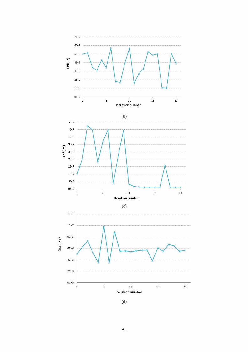
41
(b)
(c)
(d)

42
(e)
Figure 3.7 convergence behaviors of (a) objective function; (b) Exf;(c) Gxzf; (d) Etf; (e) Rxx
Further, the sweep tool in ANSYS was applied to the optimized design obtained by the
sub-problem optimization method. The number of increments of each DV: 𝑁𝑠= 10, namely,
the sweep execution takes 4 × 10 = 40 times for 4 design variables in total. After the sweep
analysis, a new optimal result for the objective variable was obtained and is shown in Table
3.8. It is noted that the improvement is now 31.9% compared to 21.7% based on Equation
(3.33). Therefore, the results after the sweep tool are much better than that after the
approximate optimization method. Figure 3.8 shows the result of sensitivity analysis of the
four design variables, which gives a further assurance of the effectiveness of the choice of the
four constitutive parameters.
Table 3.9 The best design set obtained from the sweep analysis compared with the original parameter set
Variables 𝐄𝐱𝐟(GPa) 𝐆𝐱𝐳𝐟(MPa) 𝐄𝐭𝐟(MPa) 𝐑𝐱𝐱 OBJ Improvement
of OBJ
Parameter
set in the
original
model
5.0 5.0 10.0 1.0 7.28 —
Best
design set
of sweep
method
2.69 5.33 1.25 0.997 4.96 31.9%

43
(a)
(b)
(c)
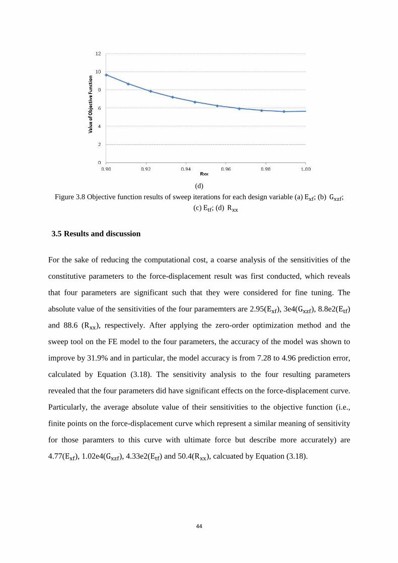
44
Figure 3.8 Objective function results of sweep iterations for each design variable (a) Exf; (b) Gxzf;
(c) Etf; (d) Rxx
3.5 Results and discussion
For the sake of reducing the computational cost, a coarse analysis of the sensitivities of the
constitutive parameters to the force-displacement result was first conducted, which reveals
that four parameters are significant such that they were considered for fine tuning. The
absolute value of the sensitivities of the four paramemters are 2.95(Exf), 3e4(Gxzf), 8.8e2(Etf)
and 88.6 (Rxx), respectively. After applying the zero-order optimization method and the
sweep tool on the FE model to the four parameters, the accuracy of the model was shown to
improve by 31.9% and in particular, the model accuracy is from 7.28 to 4.96 prediction error,
calculated by Equation (3.18). The sensitivity analysis to the four resulting parameters
revealed that the four parameters did have significant effects on the force-displacement curve.
Particularly, the average absolute value of their sensitivities to the objective function (i.e.,
finite points on the force-displacement curve which represent a similar meaning of sensitivity
for those paramters to this curve with ultimate force but describe more accurately) are
4.77(Exf), 1.02e4(Gxzf), 4.33e2(Etf) and 50.4(Rxx), calcuated by Equation (3.18).
(d)

45
3.6 Conclusion
The constitutive parameters were analyzed to result in four parameters that have significant
influence on the compressive behaviour of the cardboard. These parameters were then
fine-tuned by an optimization procedure. The optimization procedure included a zero-order
optimization algorithm and a sweep tool. After the optimization procedure, the convergent
results were achieved, and the fine-tuned parameters were obtained. As a result, the accuracy of
the model has been improved by 31.9%. The following conclusions can be drawn from the
study.
First, the optimization method combined with the sub-problem method and the sweep tool is
reliable and effective to the present problem.
Second, the procedure to remove the constitutive parameters that are of no significant influence
on the force-displacement behavior is effective. Although the analysis seems to be coarse and
ad-hoc, the subsequent optimization seems to off-set the ad-hoc analysis.
46
CHAPTER 4 MANUFACTURING IMPERFECTION ANALYSIS OF CORRUGATED
CARDBOARDS
4.1 Introduction
Manufacturing of corrugated cardboards usually introduce some significant geometric
imperfections. The materials of the cardboards are soft materials, and the control of their
geometry in manufacturing is difficult. Understanding of the robustness of the model with
respect to these imperfections is thus important. Imperfections on the geometry of the
cardboard will introduce the non-symmetric situation in particular, and this will then induce
the friction effect in the interface between the cardboard and the equipment that is placed on
the top of the cardboard. The non-symmetric situation along with the friction will introduce
the transversal movement (Figure 4.1), and this phenomenon was also observed by Sven
(2006). The objective of this chapter is to show the effect of this particular manufacturing
imperfection and its transversal movement. Section 4.2 presents the FEM model of the
cardboard system with consideration of the transversal movement and compares the model
predicted result with the experimental result of Huang (2013).
Figure 4.1 A compressed cardboard sample with transverse shear deformation

47
4.2 The Modified FEM Model of the Cardboard
First, the boundary condition that considers the transversal movement is shown in Figure 4.2,
where the movement in the transversal direction is allowed. As such, each node on the upper
liner of the cardboard has 3 DOF: two translations and one orientation, while each node on
the bottom linear is completely constrained (i.e., with the 0 DOF).
.
Figure 4.2 Free-edge boundary conditions
The shell element was employed to the four-flute model, which is with the same size as the
experimental sample of Huang (2013), with a deflection in the x-direction on the third flute
was created in the model (Figure 4.3). The deflection was made by moving a key-point in the
middle height of the third flute at coordinates 𝑥0 =𝜆
4 , 𝑦0 =
𝐻
2 (Point A in Figure 4.3) by an
amount ξ in the x-direction, which is the same idea as Lu et al. (2001). Figure 4.3 represents
the method of adding the shape imperfection. The mesh was taken the same as the one
described in Section 3.2.
Figure 4.4 shows the result calculated with the model for the different transversal movements
and the experimental result for the purpose of the comparison. From Figure 4.4, it can be seen
that the imperfection of the flute significantly affects the plastic behaviour of the cardboard,
especially the yield point. The yield points for the perfect flute, small deflection flute
(ξ = 1%) and the large deflected flute (ξ = 5%) are 185.3Mpa, 174.9Mpa and 148.0Mpa,
respectively. By changing the deflection ξ = 1% to ξ = 5%, the yield strength of the
cardboard model decreases, which was under the expectation. After the yield point, the trend

48
of the force-displacement curves with the different deflections is similar with particularly
being such that the force goes downward (notice: the force goes upward when the transversal
deflection is not considered in the FE model). This trend is in agreement with that observed
in the experiment.
Figure 4.3 Geometry of the cross section with the imperfect flute
Figure 4.4 Force-displacement curves of the FE models of corrugated cardboard with perfect flute and
imperfect flutes
The decreased yield strength in the imperfect model may be due to the buckling, further
caused by the 2D transverse deflection. In the imperfect-flute model with the 5% deflection,

49
several shapes of the cross-section of the cardboard during the compression process are
shown in Figure 4.5. From By examining Figure 4.4 and Figure 4.5 together, one can find the
cause to support the buckling mechanism for the decrease of the yield strength of the
cardboard with imperfections. First, from Figure 4.4 it can be seen that the deformation in the
x-direction occurs suddenly at the displacement of 0.76 mm. Second, from Figure 4.5, the
shape of the cross section of the cardboard does show a buckling form at the deformation of
0.76 mm.
Figure 4.5 Typical deformed shape during compression calculation on imperfect-flute model (5%
deflection)
4.3 Modeling of Friction between the Cardboard and Equipment
It is noted that when the cardboard is in operation, there will be an equipment or machine on
the top of it and the cardboard serves as a vibration isolator. There may then be a friction
between the equipment and the cardboard on their contact surface. That friction may be
significant to the behavior of the cardboard and performance of the vibration isolation with
the cardboard. In the following, the study of this friction is presented.
To model this friction with FEM, an isotropic plate is created and placed over the cardboard.
The plate is larger than the liner of the cardboard to leave a sufficient room for the plate to
slide along the top surface of the cardboard (Figure 4.6). It is noted that the testing situation
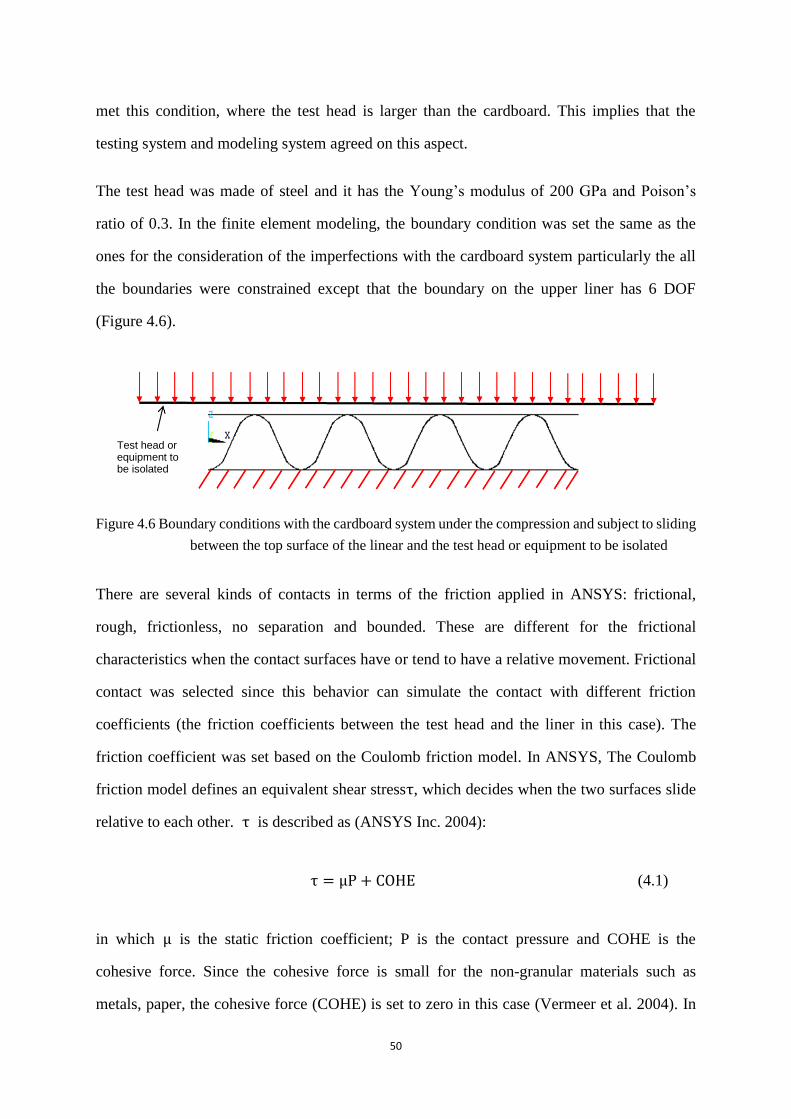
50
met this condition, where the test head is larger than the cardboard. This implies that the
testing system and modeling system agreed on this aspect.
The test head was made of steel and it has the Young’s modulus of 200 GPa and Poison’s
ratio of 0.3. In the finite element modeling, the boundary condition was set the same as the
ones for the consideration of the imperfections with the cardboard system particularly the all
the boundaries were constrained except that the boundary on the upper liner has 6 DOF
(Figure 4.6).
Figure 4.6 Boundary conditions with the cardboard system under the compression and subject to sliding
between the top surface of the linear and the test head or equipment to be isolated
There are several kinds of contacts in terms of the friction applied in ANSYS: frictional,
rough, frictionless, no separation and bounded. These are different for the frictional
characteristics when the contact surfaces have or tend to have a relative movement. Frictional
contact was selected since this behavior can simulate the contact with different friction
coefficients (the friction coefficients between the test head and the liner in this case). The
friction coefficient was set based on the Coulomb friction model. In ANSYS, The Coulomb
friction model defines an equivalent shear stressτ, which decides when the two surfaces slide
relative to each other. τ is described as (ANSYS Inc. 2004):
τ = μP + COHE (4.1)
in which μ is the static friction coefficient; P is the contact pressure and COHE is the
cohesive force. Since the cohesive force is small for the non-granular materials such as
metals, paper, the cohesive force (COHE) is set to zero in this case (Vermeer et al. 2004). In
Test head or equipment to be isolated
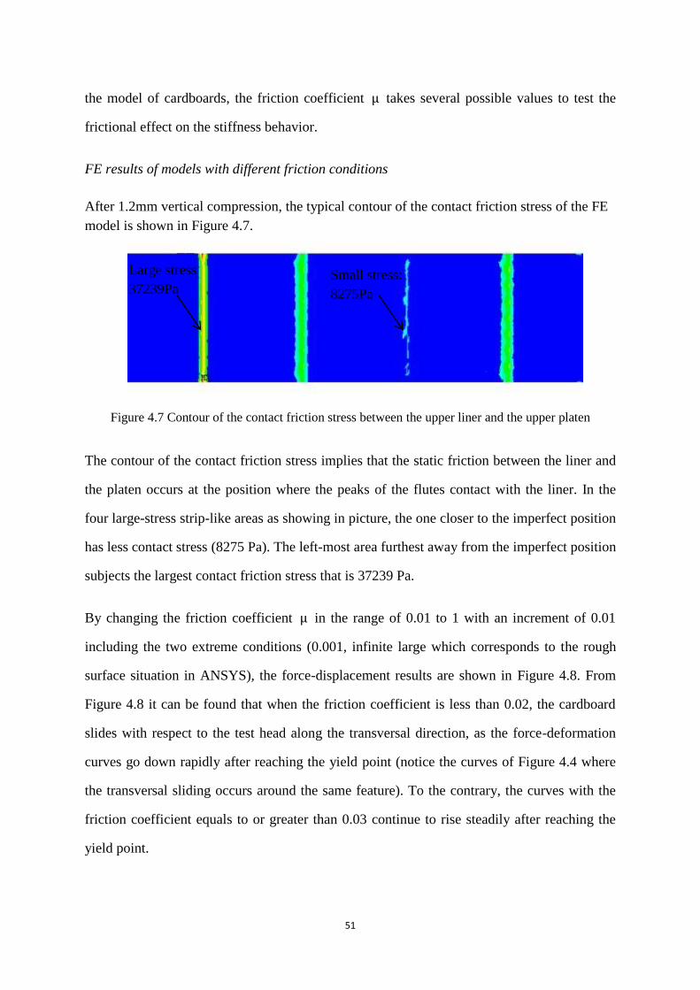
51
the model of cardboards, the friction coefficient μ takes several possible values to test the
frictional effect on the stiffness behavior.
FE results of models with different friction conditions
After 1.2mm vertical compression, the typical contour of the contact friction stress of the FE
model is shown in Figure 4.7.
Figure 4.7 Contour of the contact friction stress between the upper liner and the upper platen
The contour of the contact friction stress implies that the static friction between the liner and
the platen occurs at the position where the peaks of the flutes contact with the liner. In the
four large-stress strip-like areas as showing in picture, the one closer to the imperfect position
has less contact stress (8275 Pa). The left-most area furthest away from the imperfect position
subjects the largest contact friction stress that is 37239 Pa.
By changing the friction coefficient μ in the range of 0.01 to 1 with an increment of 0.01
including the two extreme conditions (0.001, infinite large which corresponds to the rough
surface situation in ANSYS), the force-displacement results are shown in Figure 4.8. From
Figure 4.8 it can be found that when the friction coefficient is less than 0.02, the cardboard
slides with respect to the test head along the transversal direction, as the force-deformation
curves go down rapidly after reaching the yield point (notice the curves of Figure 4.4 where
the transversal sliding occurs around the same feature). To the contrary, the curves with the
friction coefficient equals to or greater than 0.03 continue to rise steadily after reaching the
yield point.
Small stress:
8275Pa
Large stress
37239Pa

52
Figure 4.8 Calculations with different friction coefficients
4.4 Conclusions
This chapter discussed the effect of the geometrical imperfection of the corrugated cardboard
on the force-deformation relation. Closely related to this, the chapter also discussed the effect
of the friction between the cardboard and the test head. The methodology for studying the
two problems was based on modeling and simulation together with limited experimental data.
The experimental data was about the measured force-deformation relation for one sample. In
particular, the problem of geometrical imperfection was studied by assuming that there was a
transversal movement on the cardboard, that is, the different geometrical imperfections
correspond to different transversal movements. As such, by assigning a different transversal
movement on a node of the finite element on the profile of the flute (in the middle of the
profile), a different force-deformation relation can be obtained. The problem of friction was
studied by considering there is a test head or platen on the cardboard, and accordingly there is
a friction between the platen and the cardboard. The finite element model incorporating this
friction was developed, and the force-deformation relation with different friction coefficients

53
can then be found. There was also a hypothesis that the effect of the transversal movement
caused by the geometrical imperfection is also related to the friction between the cardboard
and platen.
The study concluded the following: (1) both the geometric imperfection and the friction
between the cardboard and the platen are important factors to the force-deformation relation
(compression direction), (2) the two factors are coupled, and (3) the effect of them may
greatly reduce the post-yield stiffness or the so-called flow stress of the cardboard.
54
CHAPTER 5 MODELING OF THE DAMPING IN CORRUGATED CARDBOARDS
5.1 Introduction
Damping is an important property of the cardboard when it is used for vibration isolation.
The previous work in our group did not model the damping of the cardboard instead
measured the damping (Huang 2013). The model of the damping is useful to design a
vibration isolator more accurately. In this chapter, modeling of the damping property of the
cardboard system particularly of a serial configuration is discussed. Section 5.2 will introduce
the Rayleigh damping method for modeling the damping. Section 5.3 will present the
Rayleigh model of the damping for the cardboard system. In Section 5.4, the verification of
the model will be discussed. A conclusion appears in the last section.
5.2 The Rayleigh Damping Model
The Rayleigh model of damping or simply called Rayleigh damping is the most popular
approach to represent the damping property or behavior of a system. Rayleigh damping
assumes that the damping is a linear combination of the mass and stiffness. For a general
multi-DOF system, Rayleigh damping can be expressed by
[𝐶] = 𝛼[𝑀] + 𝛽[𝐾] (5.1)
in which [C]=damping matrix; [M]= mass matrix; [K]=stiffness matrix; α and β are the
Rayleigh damping coefficients. Considering the cardboard system as a 1 DOF system, by the
orthogonal transformation, the following equation can be obtained (Chen 2013).
2𝜁𝜔 = 𝛼 + 𝛽𝜔2 (5.2)

55
As such,
𝜁 =𝛼
2𝜔+
𝛽𝜔
2 (5.3)
where 𝜔 is the natural frequency; 𝜁 is the damping ratio. To find the Rayleigh damping
coefficients α and β, one has to get at least two sets of values, namely (ζ1, ω1), (ζ2, ω2). The
subscripts 1 and 2 represent the first and second modes of vibration. As such, the following
equations find α and β (Chen 2013).
𝛽 =2𝜁1𝜔1 − 2𝜁2𝜔2
𝜔12 − 𝜔2
2 (5.4)
𝛼 = 2𝜁1𝜔1 − 𝛽𝜔12 (5.5)
5.3 Test-bed for determining 𝛇 and 𝛚
The method to determine 𝜁 and 𝜔 was based on the literature (Mallik et al. 1999). The
test-bed set-up by Huang (2013) was re-used in this thesis (Figure 5.1). A cardboard with the
length 60.8 mm, width 38 mm was taken as a specimen, and load 1.94 kg was applied to the
specimen. Two accelerometers were placed on the top of the steel block and of the vibration
exciter, respectively (Figure 5.1b). The excitation was generated and controlled by the
schematic diagram of the test-bed, as shown in Figure 5.2.
(a)
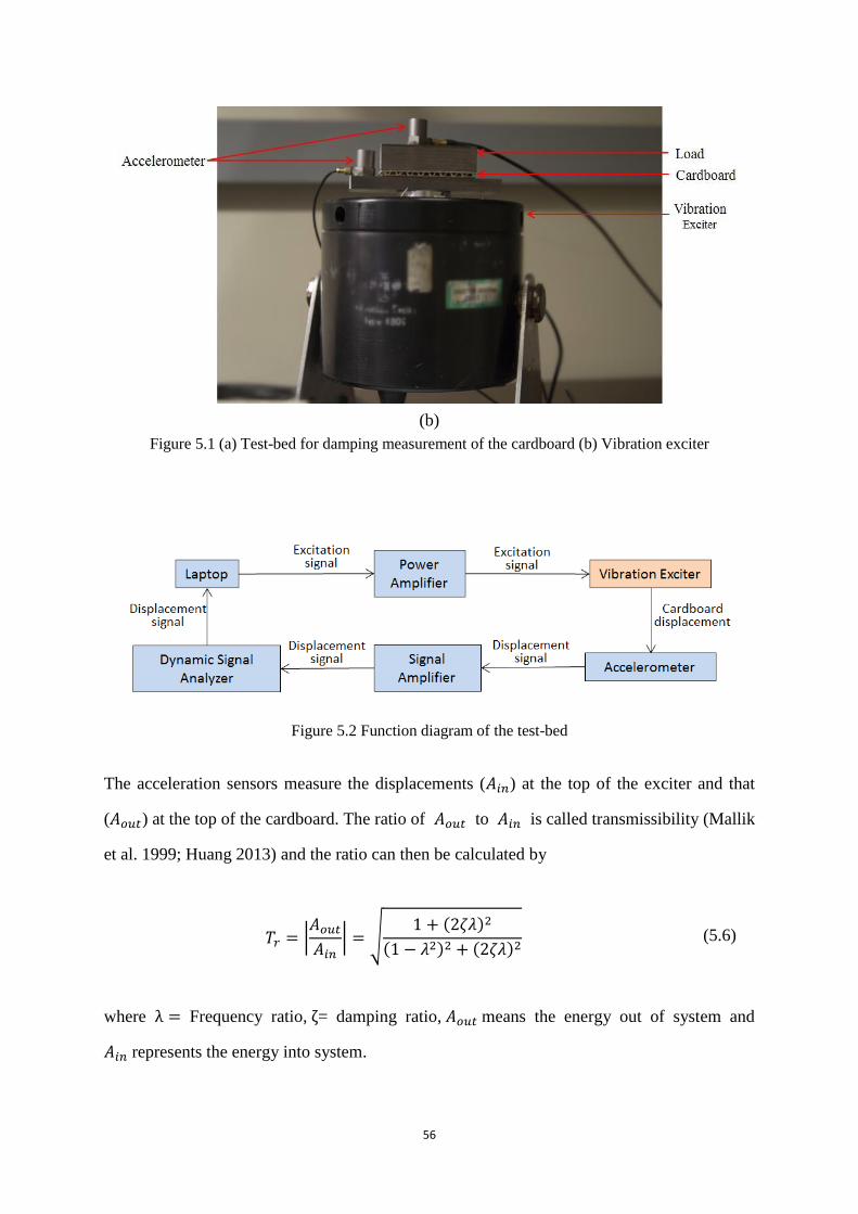
56
Figure 5.1 (a) Test-bed for damping measurement of the cardboard (b) Vibration exciter
Figure 5.2 Function diagram of the test-bed
The acceleration sensors measure the displacements (𝐴𝑖𝑛) at the top of the exciter and that
(𝐴𝑜𝑢𝑡) at the top of the cardboard. The ratio of 𝐴𝑜𝑢𝑡 to 𝐴𝑖𝑛 is called transmissibility (Mallik
et al. 1999; Huang 2013) and the ratio can then be calculated by
𝑇𝑟 = |𝐴𝑜𝑢𝑡
𝐴𝑖𝑛| = √
1 + (2𝜁𝜆)2
(1 − 𝜆2)2 + (2𝜁𝜆)2 (5.6)
where λ = Frequency ratio, ζ= damping ratio, 𝐴𝑜𝑢𝑡 means the energy out of system and
𝐴𝑖𝑛 represents the energy into system.
(b)
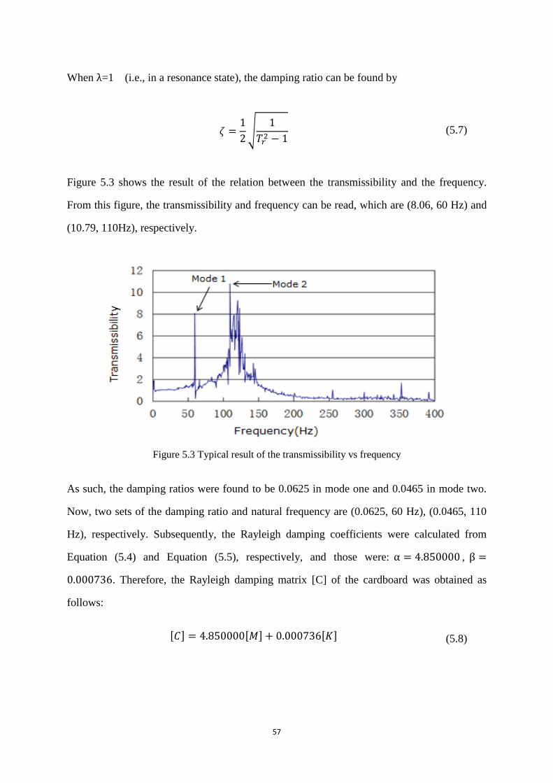
57
When λ=1 (i.e., in a resonance state), the damping ratio can be found by
𝜁 =1
2√
1
𝑇𝑟2 − 1
(5.7)
Figure 5.3 shows the result of the relation between the transmissibility and the frequency.
From this figure, the transmissibility and frequency can be read, which are (8.06, 60 Hz) and
(10.79, 110Hz), respectively.
Figure 5.3 Typical result of the transmissibility vs frequency
As such, the damping ratios were found to be 0.0625 in mode one and 0.0465 in mode two.
Now, two sets of the damping ratio and natural frequency are (0.0625, 60 Hz), (0.0465, 110
Hz), respectively. Subsequently, the Rayleigh damping coefficients were calculated from
Equation (5.4) and Equation (5.5), respectively, and those were: α = 4.850000 , β =
0.000736. Therefore, the Rayleigh damping matrix [C] of the cardboard was obtained as
follows:
[𝐶] = 4.850000[𝑀] + 0.000736[𝐾] (5.8)

58
5.4 Verification of the Damping Model
The verification of the damping model of the corrugated cardboard was carried out by means
of the test-bed, as built by Huang (2013). The schematic diagram of the test-bed is shown in
Figure 5.4a, and the schematic diagram of the signal flow is shown in Figure 5.4b.
Furthermore, a comparison of the model prediction and the experimental measurement was
made at the point of time when the resonance occurs. This is so because in the resonance
situation, the role of damping is at its maximum.
Figure 5.4 (a) the test-bed for displacement measurement in the pump-cardboard-ground vibration
system (Huang 2013) (b) the signal flow of the test.
Further, a comparison was made for both the damping coefficient, measured by Huang
(2013), and the one, proposed in this thesis, based on the Rayleigh damping model. The
(a)
(b)
Signal
Analyzer
Laptop
Vacuum
pump
Cardboards
Signal
Amplifier
Accelerometer

59
comparison was made for the transmissibility (𝑇𝑟), which was defined as the ratio of the force
(𝐹𝑇) transmitted to the ground through the cardboard to the force generated by the pump (𝐹0).
The transmissibility can be further expressed based on the definition of 𝐹𝑇 and 𝐹0 by the
stiffness, damping and frequency, which is given by
Tr =𝐹𝑇
𝐹0= {
k2 + ω2c2
(k − mω2)2 + ω2c2}
12⁄
(5.9)
where ω is the operating frequency of the pump, m is the mass of the pump, and 𝑐 is the
damping of the isolator, and k is the stiffness of the isolator.
5.4.1 Layer of the cardboard system at the resonance frequency
The cardboard system considered in this thesis was a set of cardboards that connected in
serial. It was further assumed that these cardboards are identical. Therefore, there is
(𝑐0 = 𝑐1 = ⋯ = 𝑐𝑛−1). The total or equivalent damping (𝑐𝑒𝑞𝑣) of the cardboard system is
given by (Rao and Horton 2003)
𝑐𝑒𝑞𝑣 =𝑐0
𝑛 (5.10)
Likewise, with the same stiffness (𝑘0 = 𝑘1 = ⋯ = 𝑘𝑛−1), the total or equivalent stiffness
(𝑘𝑒𝑞𝑣) of the system is expressed by (Rao and Horton 2003)
keqv =k0
n (5.11)
Let the exciting frequency ω is equal to the natural frequency of the system ω𝑛. This then
gives:
ω = ωn = 183.69 rad/s (5.12)
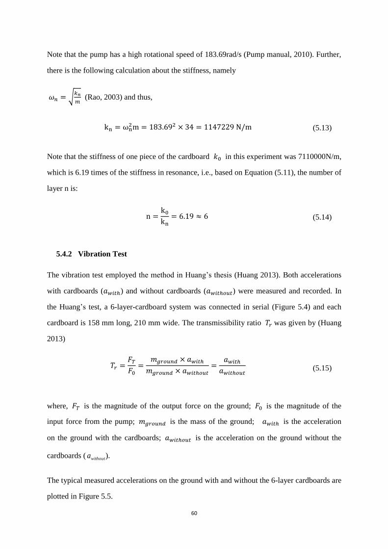
60
Note that the pump has a high rotational speed of 183.69rad/s (Pump manual, 2010). Further,
there is the following calculation about the stiffness, namely
𝜔𝑛 = √𝑘𝑛
𝑚 (Rao, 2003) and thus,
kn = ωn2m = 183.692 × 34 = 1147229 N/m (5.13)
Note that the stiffness of one piece of the cardboard 𝑘0 in this experiment was 7110000N/m,
which is 6.19 times of the stiffness in resonance, i.e., based on Equation (5.11), the number of
layer n is:
n =k0
kn= 6.19 ≈ 6 (5.14)
5.4.2 Vibration Test
The vibration test employed the method in Huang’s thesis (Huang 2013). Both accelerations
with cardboards (𝑎𝑤𝑖𝑡ℎ) and without cardboards (𝑎𝑤𝑖𝑡ℎ𝑜𝑢𝑡) were measured and recorded. In
the Huang’s test, a 6-layer-cardboard system was connected in serial (Figure 5.4) and each
cardboard is 158 mm long, 210 mm wide. The transmissibility ratio 𝑇𝑟 was given by (Huang
2013)
𝑇𝑟 =𝐹𝑇
𝐹0=
𝑚𝑔𝑟𝑜𝑢𝑛𝑑 × 𝑎𝑤𝑖𝑡ℎ
𝑚𝑔𝑟𝑜𝑢𝑛𝑑 × 𝑎𝑤𝑖𝑡ℎ𝑜𝑢𝑡=
𝑎𝑤𝑖𝑡ℎ
𝑎𝑤𝑖𝑡ℎ𝑜𝑢𝑡 (5.15)
where, 𝐹𝑇 is the magnitude of the output force on the ground; 𝐹0 is the magnitude of the
input force from the pump; 𝑚𝑔𝑟𝑜𝑢𝑛𝑑 is the mass of the ground; 𝑎𝑤𝑖𝑡ℎ is the acceleration
on the ground with the cardboards; 𝑎𝑤𝑖𝑡ℎ𝑜𝑢𝑡 is the acceleration on the ground without the
cardboards ( withouta ).
The typical measured accelerations on the ground with and without the 6-layer cardboards are
plotted in Figure 5.5.

61
Figure 5.5 Measurement results
In this test, only the acceleration at the frequency of 29.25 Hz (183.69 rad/s) was measured
as the frequency was the operation frequency of the pump. The measured accelerations
transmitted from the pump with and without cardboards to the ground at 29.25 Hz are
1.11 × 10⁻⁹ m/s2 and 3.43 × 10⁻¹⁰ m/s2, respectively.
Thus, based on Equation (5.15), the transmissibility of the 6-layer cardboards is
Tr =1.11 × 10⁻⁹
3.43 × 10−10= 3.24 (5.16)
By repeating the measurements, the mean transmissibility
Tr = 3.28
5.4.3 Comparison
In Huang’s work, the damping of the system with 1-layer cardboard was 861 Ns/m . Based
on Equation (5.10), the damping (c) of the 6-layer cardboard system is 143.5 Ns/m .
Likewise, the stiffness of the system with 1-layer cardboard is 7110000 N/m. Based on
Equation (5.11), the stiffness (k) of the 6-layer cardboard system is 1185000 N/m. The
1.11e-9 m/s2
3.43e-10 m/s2

62
mass m = 34kg and the frequency ω = 183.69 rad/s (Pump manual, 2010). Substituting
the values of c, k, m and ω into Equation (5.9) yields to:
Tr = {11850002 + 183.692 × 143.52
(1185000 − 34 × 183.692)2 + 183.692 × 143.52}
12⁄
= 25.73 (5.17)
The Rayleigh damping model of the cardboards is obtained in Equation (5.8). Substituting the
same stiffness and the same mass as that in Huang’s model into Equation (5.8) leads to:
c = 1036.6 Ns/m (5.18)
Thus, the transmissibility calculated by using the Rayleigh damping is
Tr = {11850002 + 183.692 × 1036.62
(1185000 − 34 × 183.692)2 + 183.692 × 1036.62}
12⁄
= 6.18 (5.19)
The transmissibility calculated using the damping in Huang’s work has an error of 87%,
while the transmissibility calculated by the Rayleigh damping developed in this thesis has the
error of 47%. Therefore, the transmissibility calculated by the Rayleigh damping is more
accurate.
5.5 Conclusion
In this chapter, the Rayleigh damping model was developed for the cardboards in this thesis.
Two constant coefficients α and β in the Rayleigh damping were determined by the
experiment. The verification was conducted by the pump-cardboard-ground vibration system.
The result concluded that the Rayleigh damping is more accurate than the Huang’s
measurement based approach.

63
CHAPTER 6 CONCLUSION AND FUTURE WORK
6.1 Overview
This thesis presented a study on improving the method for calculating the stiffness and
damping of the corrugated cardboard for the vibration isolation application. There are many
studies on the properties of stiffness and damping and the models of them. Recently, Huang
(2013) first studied the stiffness and damping of the corrugated cardboards for the vibration
isolation application. However, there are some shortcomings both in Huang’s and in others’
as follows.
(1) The accuracy of the models for stiffness and damping is not very high. One plausible
cause may be due to the difficulty to determine some constitutive parameters in the
cardboard. Yet, another reason is that some physics are not taken into account in the
model, e.g., the geometrical imperfection and friction between the cardboard and the
equipment to be isolated.
(2) The damping of the cardboard is not modelled, which may give some inaccuracy in
the design of the isolation system with the cardboards.
This thesis was motivated by overcoming the foregoing shortcomings. Particularly, the first
work of the thesis was to determine the constitutive parameters more accurately by applying
the system identification technique, which was described in Chapter 3. The second work of
the thesis was to model the geometrical imperfection and friction between the cardboard and
the equipment, which was described in Chapter 4. The third work of the thesis was to model
the damping of the cardboard, which was described in Chapter 5.
The following are conclusions drawn from this thesis:

64
(1) The constitutive parameters are indeed very important to the accuracy of the
modelling for the stiffness in the compression direction or the force-deformation
relation in the vertical direction, which made FEM prediction more accurate.
Accuracy of prediction increased by 31.9% after applying the parameter identification
procedure compared to the accuracy of the model in Huang’s thesis (Huang 2013).
(2) The geometrical imperfection of the cardboard and friction between the cardboard and
equipment are very important factors to the accuracy of the modeling for the stiffness
as well. Generally, less deflection of flute or greater interface friction coefficient
result in a stronger yield strength of the cardboard. These two factors are coupled to
affect the post-yield stiffness by giving rise to transversal movement.
(3) The Rayleigh model for the damping of the cardboard has a sufficient accuracy for the
cardboard by decreasing the error from 87% to 47%. Thus, the Rayleigh damping
contributes to the accuracy of the isolation system considerably.
6.2 Contributions
The main contributions of the thesis are summarized in the following:
(1) The provision of an effective procedure to determine the constitutive parameters
more accurately via a system identification technique. Through a simple compression
testing, these parameters were determined. This procedure can readily be applied to
other similar problems.
(2) The finding that the geometrical imperfection and friction between the cardboard and
equipment are coupled and these have a significant effect on the accuracy of the
model for the stiffness of the cardboard.

65
(3) The provision of a model for the damping of the cardboard that could be used to
design the isolation system of cardboards more accurately.
6.3 Future Work
There are a number of potential works worthy of further investigation. The following are
some of these possible works:
First, the different optimization algorithms can be applied in the optimization of the
constitutive parameters in the FE model of the corrugated cardboards, such as genetic
algorithm and the first-order method. This may provide more options for identifying the
material parameters based on the different requirements of accuracy and computational cost.
Second, the objective function in the optimization model in this thesis is formed based on the
average values of the force and displacement in the experiment. Other features such as the
stress field can be considered as the objective function.
Third, the geometrical imperfections in the out-of-plain direction and even the 3-D
imperfection need to be studied more thoroughly and experimentally
Finally, the horizontal movement of the vacuum pump can be considered in the damping
models.

66
REFERENCES
Aboura, Z., N. Talbi, S. Allaoui, and M. L. Benzeggagh. 2004. Elastic behavior of corrugated
cardboard: experiments and modeling. Composite Structures 63:53–62.
Allansson, A., and B. Svärd. 2001. Stability and collapse of corrugated board. Unpublished
M.Sc. thesis. Structural Mechanics. Lund University, Lund, Sweden.
ANSYS Inc. 2004. Theory Reference. Canonsburg , PA.
ANSYS Inc. 2005. ANSYS Advanced Analysis Techniques Guide, Ansys Help. Canonsburg,
PA.
Baum, G. A., D. C. Brennan, and C. C. Habeger. 1981. Orthothopic elastic constants of paper.
Tappi 64:97–101.
Biancolini, M. E. 2005. Evaluation of equivalent stiffness properties of corrugated board.
Composite Structures 69:322–328.
Biancolini, M. E., and C. Brutti. 2003. Numerical and experimental investigation of the
strength of corrugated board packages. Packaging Technology and Science 16:47–60.
Budynas, R. G. 1999. Advanced Strength and Applied Stress Analysis (2nd ed.).
McGraw-Hill, Boston.
Carlsson, L. a., T. Nordstrand, and B. Westerlind. 2001. On the elastic stiffnesses of
corrugated core sandwich. Journal of Sandwich Structures and Materials 3:253–267.
Chen, W. 2013. Development of a kinetic model for loop-free colonoscopy technology.
Unpublished Ph.D. thesis. University of Saskatchewan, Saskatoon, SK, Canada.
Dayyani, I., S. Ziaei-Rad, and H. Salehi. 2011. Numerical and experimental investigations on
mechanical behavior of composite corrugated core. Applied Composite Materials 19:705–
721.
De Silva, C. W. 2006. Vibration: fundamentals and practice (2nd ed.). CRC press, Boca
Raton.
Gilchrist, A. C., J. C. Suhling, and T. J. Urbanik. 1998. Nonlinear finite element modeling of
corrugated board. Mechanics of Cellulosic Materials ASME 231:101–106.
67
Haj-Ali, R., J. Choi, B.-S. Wei, R. Popil, and M. Schaepe. 2009. Refined nonlinear finite
element models for corrugated fiberboards. Composite Structures 87:321–333.
Hammou, A. D., P. T. Minh Duong, B. Abbès, M. Makhlouf, and Y.-Q. Guo. 2012.
Finite-element simulation with a homogenization model and experimental study of free drop
tests of corrugated cardboard packaging. Mechanics & Industry 13:175–184.
Huang, J. 2013. Investigation of corrugated cardboard for vibration isolation. Unpublished
M.Sc. thesis. University of Saskatchewan, Saskatoon, SK, Canada.
Imaoka, S. 2000. ANSYS tips & tricks: structure shell elements, part 1. Redondo beach,
California, USA.
Jiménez-Caballero, M. A., I. Conde, B. García, and E. Liarte. 2009. Design of different types
of corrugated board packages using finite element tools. SIMULIA Customer Conference.
London, UK.
Kirwan, M. J. 2012. Handbook of Paper and Paperboard Packaging Technology (2nd ed.).
John Wiley & Sons, London, UK.
Krusper, A., P. Isaksson, and P. Gradin. 2008. Modeling of out-of-plane compression loading
of corrugated paper board structures. Journal of Engineering Mechanics 133:1171–1177.
Lu, T. J., C. Chen, and G. Zhu. 2001. Compressive behaviour of corrugated board panels.
Journal of Composite Materials 35:2098–2126.
Mallik, A. K., V. Kher, M. Puri, and H. Hatwal. 1999. On the modelling of non-linear
elastomeric vibration isolators. Journal of Sound and Vibration 219:239–253.
Mann, R. W., G. A. Baum, and C. C. Habeger Jr. 1979. Determination of all nine orthotropic
elastic constants for machine-made paper. Tappi 63:163–166.
Nguyen, M. Q., S. S. Jacombs, R. S. Thomson, D. Hachenberg, and M. L. Scott. 2005.
Simulation of impact on sandwich structures. Composite Structures 67:217–227.
Nordstrand, T. 2003. Basic testing and strength design of corrugated board and containers.
Unpublished Ph.D. thesis. Lund University, Lund, Sweden.
Nordstrand, T. M. 1995. Parametric study of the post-buckling strength of structural core
sandwich panels. Composite Structures 30:441–451.
Nordstrand, T. M., and L. A. Carlssonb. 1997. Evaluation of transverse shear stiffness of
structural core sandwich plates. Composite Structures 8223:145–153.

68
Patel, P., T. Nordstrand, and L. A. Carlssonb. 1997. Local buckling and collapse of
corrugated board under biaxial stress. Composite Structures 39:93–110.
Pommier, J. C., J. Poustis, E. Fourcade, and P. Morlier. 1991. Determination of the critical
load of a corrugated box subjected to vertical compression by finite element methods.
Proceedings of the 1991 International Paper Physics Conference (pp. 437–447). Kona, HI.
Rajesh, E., and M. Sivaprakash. 2013. Analysis of friction factor by employing the ring
compression test under different lubricants. International Journal of Advancements in
Research & Technology 4:1163–1171.
Rao, S. S., and M. J. Horton. 2003. Mechanical Vibrations (5th ed.). Prentice Hall, Upper
Saddle River.
Schwingshackl, C. W., G. S. Aglietti, and P. R. Cunningham. 2006. Determination of
honeycomb material properties: existing theories and an alternative dynamic approach.
Journal of Aerospace Engineering 19:177–183.
Sek, M. 2009. Dynamic Response of a Multilayer Corrugated Structure with
History-Dependent Properties Subjected to Transient Loads. Proceedings of SEM 2009
Annual Conference on Experimental and Applied Mechanics (pp. 1–3). Albuquerque NM,
USA.
Standard Specification for Corrugated and Solid Fiberboard Sheet Stock ( Container Grade )
and Cut Shapes. ASTM standard D4727. 2007.
Stenberg, N. 2003. A model for the through-thickness elastic–plastic behaviour of paper.
International Journal of Solids and Structures 40:7483–7498.
Talbi, N., A. Batti, R. Ayad, and Y. Q. Guo. 2009. An analytical homogenization model for
finite element modelling of corrugated cardboard. Composite Structures 88:280–289.
Thakkar, B. K., L. G. J. Gooren, R. H. J. Peerlings, and M. G. D. Geers. 2008. Experimental
and numerical investigation of creasing in corrugated paperboard. Philosophical Magazine
88:3299–3310.
Twede, D., and S. E. M. Selke. 2005. Cartons, Crates and Corrugated Board: Handbook of
Paper and Wood Packaging Technology. DEStech Publications, Inc, Lancaster.
Vermeer, P. A., W. Ehlers, H. J. Hermann, and E. Ramm. 2004. Modelling of
Cohesive-Frictional Materials: Proceedings of Second International Symposium on
Continuous and Discontinuous Modelling of Cohesive-Frictional Materials. CRC Press,
Stuttgart.