ENERGY SINKS WITH NONLINEAR STIFFNESS AND NONLINEAR DAMPING

ABSTRACT

Title of Thesis: ENERGY SINKS WITH NONLINEAR STIFFNESS AND NONLINEAR DAMPING

Matthew Charles Colvin, Master of Science, 2010 Thesis directed by: Professor Amr Baz Department of Mechanical Engineering

Nonlinear energy sinks (NES) have been shown to be effective for vibration

attenuation under certain conditions. The effects of coupling linear systems to NES with

nonlinear stiffness and linear damping have been extensively investigated. However,

research involving nonlinearly damped NES is minimal. In this thesis, the performance

of nonlinearly damped NES are examined and comparisons are made with the

performance of linearly damped counterparts. Saddle-node and Hopf bifurcation

diagrams are presented to show instabilities of solutions. The strongly modulated

response (SMR), which exists only near 1:1 resonance between the forcing frequency and

the frequency of the linear system, is investigated as well. Finally, time response

comparisons are made between the systems with linearly and nonlinearly damped NES.

ENERGY SINKS WITH NONLINEAR STIFFNESS AND NONLINEAR DAMPING

by

Matthew Charles Colvin

Thesis submitted to the Faculty of the Graduate School of the University of Maryland, College Park in partial fulfillment

of the requirements for the degree of Master of Science

2010 Advisory Committee: Professor Amr Baz, Chair Professor Balakumar Balachandran Professor Nikhil Chopra

©Copyright by

Matthew Charles Colvin

2010

ii

To my parents, William and Linda

iii

TABLE OF CONTENTS

1.0 Introduction .............................................................................................................. 1

1.1 Overview .............................................................................................................. 1

1.2 Summary of Related Literature ............................................................................ 1

1.3 Comparison of Nonlinear Energy Sinks with Linear Vibration Absorbers ....... 21

1.4 Experiments Related to NES .............................................................................. 25

1.5 Outline of this Thesis ......................................................................................... 30

1.6 Summary ............................................................................................................ 30

2.0 Concept Energy Sinks with Nonlinear Stiffness and Damping ............................. 32

2.1 Introduction ........................................................................................................ 32

2.2 Description of Considered Systems ................................................................... 32

2.3 Analysis of the Different Systems ...................................................................... 34

2.3.1 Linear System ............................................................................................. 34

2.3.2 NES System ................................................................................................ 34

2.3.3 Nonlinear System with Nonlinear Damping ............................................... 35

2.4 Performance Comparisons ................................................................................. 36

2.5 Summary ............................................................................................................ 40

2.A Appendix ............................................................................................................ 41

3.0 Nonlinear Analysis of Nonlinear Energy Sinks ..................................................... 44

3.1 Introduction ........................................................................................................ 44

3.2 Saddle-Node Bifurcation .................................................................................... 45

3.2.1 Saddle-Node Bifurcation Background ........................................................ 45

3.2.2 Saddle-Node Bifurcation Analysis for the Linearly Damped System ........ 48

3.2.3 Saddle-Node Bifurcation Analysis for the Nonlinearly Damped System .. 51

3.2.4 Discussion of Results for Saddle-Node Bifurcations.................................. 55

3.3 Hopf Bifurcation ................................................................................................ 56

3.3.1 Hopf Bifurcation Background..................................................................... 56

3.3.2 Hopf Bifurcation Analysis for the System with Linear Damping .............. 60

3.3.3 Hopf Bifurcation Analysis for the System with Nonlinear Damping ......... 65

3.3.4 Discussion of Results for Hopf Bifurcations .............................................. 69

3.4 Conclusions ........................................................................................................ 72

iv

3.A Appendix ............................................................................................................ 73

3.A.1 Saddle-Node Bifurcation Equation Derivations (Linear Damping) ........... 73

3.A.2 Saddle-Node Bifurcation Equation Derivations (Nonlinear Damping) ...... 80

3.A.3 Saddle-Node Bifurcation Analysis Digressions.......................................... 89

3.A.4 Hopf Bifurcation Equation Derivations (Linear Damping) ........................ 93

3.A.5 Hopf Bifurcation Equation Derivations (Nonlinear Damping) .................. 96

3.A.6 Hopf Bifurcation Analysis Digressions .................................................... 100

3.A.7 MATLAB Code ........................................................................................ 103

4.0 Strongly Modulated Response (SMR) ................................................................. 166

4.1 SMR Introduction ............................................................................................. 166

4.2 SMR Analysis for the System with Linear Damping ....................................... 166

4.2.1 Slow Invariant Manifold (SIM) Projection (Linear Damping) ................. 166

4.2.2 Phase Portraits (Linear Damping) ............................................................. 170

4.2.3 1-D Mapping (Linear Damping) ............................................................... 173

4.3 SMR Analysis for the System with Nonlinear Damping ................................. 177

4.3.1 Slow Invariant Manifold (SIM) Projection (Nonlinear Damping) ........... 177

4.3.2 Phase Portraits (Nonlinear Damping) ....................................................... 181

4.3.3 1-D Mapping (Nonlinear Damping) ......................................................... 184

4.4 Discussion of Results for SMR ........................................................................ 188

4.A Appendix .......................................................................................................... 190

4.A.1 SMR Equation Derivations (Linear Damping) ......................................... 190

4.A.2 SMR Equation Derivations (Nonlinear Damping) ................................... 209

4.A.3 Method of Creating 1-D Maps .................................................................. 233

4.A.4 MATLAB Code ........................................................................................ 234

5.0 Time Response Analysis of the Nonlinear Energy Sink ...................................... 260

5.1 Introduction ...................................................................................................... 260

5.2 System Performance when Subjected to Impulse Loading .............................. 260

5.3 System Performance Comparisons Using Poincaré Maps ............................... 268

5.3.1 Background on Poincaré Sections and Maps ............................................ 268

5.3.2 Analysis of the Linearly and Nonlinearly Damped Systems using Phase Portraits and Poincaré Maps ................................................................................... 273

5.3.3 Discussion of Phase Portraits and Poincaré Maps of the Linearly and Nonlinearly Damped Systems................................................................................. 279

v

5.4 Conclusions ...................................................................................................... 280

5.A Appendix .......................................................................................................... 281

5.A.1 MATLAB Code for Time Response Simulations ..................................... 281

5.A.2 MATLAB Code for Phase Portrait and Poincaré Examples ..................... 285

5.A.3 MATLAB Code for Phase Portraits .......................................................... 286

5.A.4 MATLAB Code for Poincaré Maps .......................................................... 287

6.0 Conclusions and Recommendations .................................................................... 289

6.1 Summary of Work Presented ........................................................................... 289

6.2 Suggested Future Work .................................................................................... 291

6.3 Practical Applications of Nonlinear Energy Sinks ........................................... 292

7.0 References ............................................................................................................ 293

1

1.0 Introduction

1.1 Overview

Mechanical vibration has undesirable effects in many engineering applications including

machine tool operation, earthquake isolation of buildings, electronic packaging, and

aerospace structures, to name a few. Linear isolation methods have been developed to

help mitigate these problems. However, recent advancements show that, depending on

the application, nonlinear energy sinks (NES) can be far more effective in vibration

attenuation than linear absorbers. In fact, nonlinear targeted energy transfer (TET), the

main motive for attaching a NES, was “first observed by Gendelman (2001) who studied

the transient dynamics of a two-DOF system consisting of a damped linear oscillator that

was weakly coupled to an essentially (strongly) nonlinear, damped attachment” (Vakakis

et al., 2008). Clearly, the study of NES is still in its infancy, but the concept has already

been shown effective in vibration mitigation under certain conditions. Fundamentally, a

NES is nothing more than a mass attached to a primary system with a nonlinear spring

and a linear or nonlinear damper.

This chapter begins by presenting an overview of earlier works related to NES.

General comparisons between classical linear vibration absorbers and NES are then

discussed, followed by a summary of related experiments. Finally, an overview of the

topics discussed in this thesis is presented at the end of the chapter.

1.2 Summary of Related Literature

Targeted energy transfer (TET) can be broadly defined as the case when “energy of some

form is directed from a source (donor) to a receiver (recipient) in a one-way irreversible

2

fashion” (Vakakis et al., 2008). In the case of a nonlinear energy sink (NES) attached to

a linear system, TET refers to the irreversible transfer of energy from the linear system to

the NES, hence the name “sink”. This process of TET is also referred to as energy

pumping.

Energy pumping from an impulsively loaded linear system to a strongly nonlinear

(incapable of being linearized) attachment was investigated by Vakakis (2001) by

assuming the linear system to be a chain of elastically interconnected particles. Initially,

Vakakis introduced energy pumping concepts by application to an impulsively loaded

two-degree of freedom system given by

0, 0 0 0

, 0 0 0.

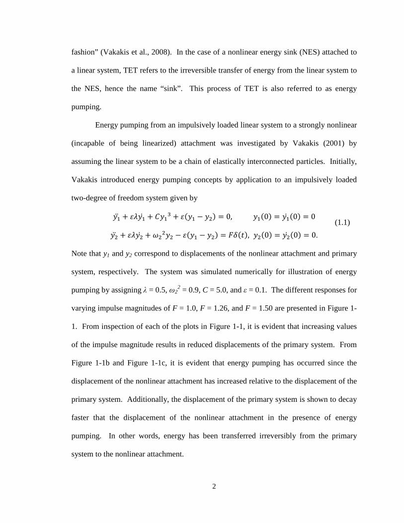
Note that y1 and y2 correspond to displacements of the nonlinear attachment and primary

system, respectively. The system was simulated numerically for illustration of energy

pumping by assigning λ = 0.5, ω22 = 0.9, C = 5.0, and ε = 0.1. The different responses for

varying impulse magnitudes of F = 1.0, F = 1.26, and F = 1.50 are presented in Figure 1-

1. From inspection of each of the plots in Figure 1-1, it is evident that increasing values

of the impulse magnitude results in reduced displacements of the primary system. From

Figure 1-1b and Figure 1-1c, it is evident that energy pumping has occurred since the

displacement of the nonlinear attachment has increased relative to the displacement of the

primary system. Additionally, the displacement of the primary system is shown to decay

faster that the displacement of the nonlinear attachment in the presence of energy

pumping. In other words, energy has been transferred irreversibly from the primary

system to the nonlinear attachment.

(1.1)

3

Figure 1-1. Time response plots for (a) F = 1.0, (b) F = 1.26, and (c) F = 1.5. Primary System: - - - - - -, Nonlinear Attachment: ----------- (Vakakis, 2001 and Gendelman et al., 2001)

(a)

(b)

(c)

4

The concepts from Vakakis (2001) are then extended to a more complex system,

consisting of a linear chain with 101 particles and a strongly nonlinear attachment at one

end, as shown in Figure 1-2. The system is impulsively loaded on the fourth particle of

the linear chain, thus the equations of motion with initial conditions are

0

0

2 0, 3, ∞

0 0 0, !0 0, ! 0 !, " #. Vakakis (2001) graphically presented the numerical results for varying values of the

linear coupling stiffness between particles, d, and for different values of the grounding

stiffness parameter, ω22. The case without energy pumping is shown in Figure 1-3, in

which the nonlinear attachment displacement decays at approximately the same time as

the linear system. In contrast, energy pumping does occur in Figure 1-4. By decreasing

the linear oscillator grounding stiffness to 0.4, the response decays faster than in the

previous case with ω22 = 0.9. In addition, the response of the nonlinear attachment

decays after the response of the linear system, indicating that there has been an

irreversible transfer of energy to the attachment. Keeping ω22 = 0.4, the coupling

stiffness between particles is increased to 3.5 for the responses shown in Figure 1-5. The

results shown in Figure 1-5 are very close to those shown in Figure 1-4, again indicating

that energy pumping has occurred. Vakakis (2001) then showed that the analysis of

energy pumping in the multi-degree of freedom system could be reduced to an analysis of

a two-degree of freedom system due to in-phase vibration of the chain of particles.

(1.2)

5

Figure 1-2. Depiction of system in equations (1.2); (Vakakis, 2001)

Figure 1-3. Time response plots for (a) the particle of the linear system adjacent to the nonlinear attachment and (b) the nonlinear attachment. Parameters are

ε = 0.1, λ = 0.5, C = 5.0, d = 3.5, and ω22 = 0.9 (Vakakis, 2001).

(a)

(b)

6





(a)

(b)

(a)

(b)

7

The effects of attaching a NES to a linear system with (N+1) degrees of freedom

by means of a spring with low stiffness are studied by Vakakis et al. (2003). Refer to

Figure 1-6 for a schematic of the system. In their study, Vakakis et al. (2003) focus on

the nonlinear normal modes (NNMs) of a conservative system in order to explain the

dynamics of the same system with damping. The NNMs are defined as “the free periodic

and synchronous oscillations of the undamped, unforced system, that are, in essence, the

non-linear analogs of the linear modes of classical vibration theory” (Vakakis et al.,

2003). In other words, the NNMs define the shape of the vibrating nonlinear system at

specific frequencies. In addition, it was shown that if damping and impulse forcing are

included in the system, the NES can vibrate at a different frequency than the linear

substructure at any given instant prior to reaching steady-state oscillations. During this

transient period, provided the external forcing is high enough, energy pumping can occur.

Energy pumping in multi-degree of freedom systems is due to resonance capture

cascades, defined as “a sequence of multiple resonance interactions of the non-linear

attachment with more than one modal oscillators of the linear substructure” (Vakakis et

al., 2003). When multiple modes of the system are excited during transient vibrations,

the attachment is able to resonate with these different modes due to its nonlinearity. In

contrast, a linear vibration absorber only has one frequency with which it can resonate,

greatly limiting the design options compared to those available when designing a NES.

8

Figure 1-6. Depiction of system studied by Vakakis et al. (2003)

Although similar to the resonance capture cascades of multi-degree of freedom

linear systems with NES, resonance capture in single-degree of freedom systems omits

the word “cascades” because there is only one linear natural frequency with which to

resonate. In order to understand resonance capture, the concept of resonance manifold

must first be grasped. Vakakis et al. (2008) reference Sanders and Verhulst (1985) by

introducing the following damped nonlinear “system in polar form with multiple phase

angles”:

%& '(, % , % '!

(& % , ( )*,

where I “represents energy-like amplitudes” (Vakakis et al., 2008), and ( is a “vector of

angles” (Vakakis et al., 2008). The vector I has length p, and the vector ( has length q.

The set of p positive real numbers is represented by '!, and the q-torus, or the torus

requiring q “angular coordinates to describe the motion” (Nayfeh and Balachandran,

(1.3)

9

1995), is represented by )*. The frequency vector is given by

% +% , % , … , *% -..

Vakakis et al. (2008) define a resonance manifold as “the set of points in / '! where

% 0 0, 1,2, … 2”. In other words, a resonance manifold is the set of points in D

for which all frequencies are identical to zero. Resonance capture can be divided into

two types: Transient Resonance Capture (TRC) and Sustained Resonance Capture (SRC).

Vakakis et al. (2008) define TRC “as capture into a resonance manifold which occurs and

continues for a certain period of time, followed by a transition to escape from capture”.

On the other hand, SRC is “defined as resonance capture that will never escape with

increasing time” (Vakakis et al., 2008). When observing a phase portrait, resonance

capture occurs when the trajectory of the system becomes attracted and locked to the

resonance manifold. In the case of a single-degree of freedom linear system coupled to a

NES, significant amounts of energy can be exchanged between the two oscillators during

resonance capture as illustrated by the concept of targeted energy transfer.

The effect of resonance capture on targeted energy transfer (TET) is illustrated in

an example by Lee et al. (2008) of an impulsively loaded system. The system,

3 43 3 3 5 3 5 0

65 5 3 5 3 0,

is given parameters ω02 = k1/m1 = 1, C = k2/m2 = 1, ϵ = m2/m1 = 0.05, λ1 = c1/m1 = 0.0015,

λ2 = c2/m2 = 0.0015. Lee et al. (2008) discuss three different ways in which targeted

energy transfer (TET) can occur: fundamental TET, subharmonic TET, and TET initiated

by non-linear beating. In the case of fundamental TET, “the linear oscillator and the

non-linear attachment oscillate with identical frequencies in the neighbourhood of the

(1.5)

(1.4)

10

fundamental frequency ω0” (Lee et al., 2008). Figure 1-7 presents percentages of energy

transfer to and energy dissipation by the NES. As seen from Figure 1-7, almost all of the

energy is eventually transferred to the NES. Corresponding to the trend of energy

transfer to the NES is the trend of energy dissipated by the NES. From these two plots, it

can be seen that after some initial transients, the NES effectively dissipates over 70% of

the total energy in the system. For illustration of the conditions at which this energy

pumping occurs, Figure 1-8 presents frequency-energy plots versus the total system

energy in the form of wavelet transforms (WTs). The darker regions represent high

amplitudes of the WT, and the lighter regions depict the opposite. Refer to Vakakis et al.

(2008) for detailed discussions on the use of WTs. As seen from the contour plots, as the

energy in the system increases, the frequency of the linear system and NES tend to unity,

indicating that 1:1 resonance capture is responsible for this type of TET.

Figure 1-7. Fundamental TET. Percentage of the total energy versus time for energy transfer to the NES and energy dissipation by the NES (Lee et al., 2008).

11

Figure 1-8. Fundamental TET. Contour plots of WTs depicting the frequency-energy dependence of the primary system and the NES (Lee et al., 2008).

The second way in which TET can occur is through subharmonic TET.

Subharmonic TET refers to exciting “families of NNMs of the underlying Hamiltonian

system with the nonlinear attachment engaging in m:n internal resonance with the linear

oscillator (LO) (where m, n are integers with m < n)” (Vakakis et al., 2008). A

Hamiltonian system is defined by the following relations (Nayfeh and Balachandran,

1995):

2 898!: , # 898*: , 1,2, … , ;, < <2, 2, … 2=, #, #, … #=, . Internal resonance refers to the condition where the linear natural frequencies, ωi, of a

system are integer multiples of each other. In other words, “there exist positive or

negative integers m1, m2, m3, …, mn such that m1ω1 + m2ω2 + m3ω3 +…+ mnωn > 0”

(Nayfeh and Mook, 1995). Lee et al. (2008) continue the numerical simulation by

showing results for the case of subharmonic TET with a 1:3 resonance capture, that is,

the primary system “oscillates with a frequency approximately three times that of the

NES” (Vakakis et al., 2008). Figure 1-9 presents percentages of energy transfer to and

energy dissipation by the NES. From inspection of the plot of energy transfer to the

(1.6)

12

NES, approximately 70% of the total system energy is transferred to the NES. As

opposed to the case of fundamental TET, Figure 1-10 shows the frequency localized to

approximately 1/3 for the NES and unity for the primary system.

Figure 1-9. Subharmonic TET. Percentage of the total energy versus time for energy transfer to the NES and energy dissipation by the NES (Lee et al., 2008).

Figure 1-10. Subharmonic TET. Contour plots of WTs depicting the frequency-energy dependence of the primary system and the NES (Lee et al., 2008).

In order for fundamental TET and subharmonic TET to occur in an impulsively

loaded system, TET must be initiated by nonlinear beating. As reasoned by Lee et al.

(2008), fundamental TET and subharmonic TET “cannot be activated with the NES at

rest, since in both cases the motion is initialized from a non-localized state of the

13

system”. Figure 1-11 illustrates one case of the energy exchanges during nonlinear beat

phenomena in an undamped system. As seen from the plots, the energy in the primary

system is a mirror image (about a horizontal axis at 50%) of the energy in the NES,

indicating a direct energy exchange between the two. As this energy transfer is clearly

reversible, introduction of damping in the system is required for the exchange to be final.

With damping in the system and after establishing in the response “an initial non-linear

beat phenomenon, either one of the main (fundamental or subharmonic) TET

mechanisms can be activated by a non-linear transition (jump) in the dynamics” (Lee et

al., 2008). By inspection of the percentage of total energy in the NES as shown in Figure

1-12, the nonlinear beat phenomena is seen early in the motion as the energy percentage

fluctuates greatly before converging. Once the nonlinear beating has subsided,

fundamental TET increases energy in the NES to nearly 100% of the total system energy.

As evident from Figure 1-13, the 1:1 resonance (i.e. fundamental TET) is the means of

energy pumping in this case.

Figure 1-11. Example of energy exchanges due to nonlinear beat phenomena (Lee et al., 2008).

14

Figure 1-12. Initiating TET. Percentage of the total energy versus time for energy transfer to the NES and energy dissipation by the NES (Lee et al., 2008).

Figure 1-13. Initiating TET. Contour plots of WTs depicting the frequency-energy dependence of the primary system and the NES (Lee et al., 2008).

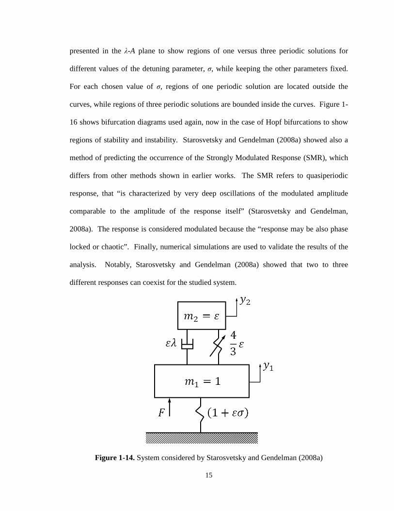
Of particular interest to this thesis is the work presented in Starosvetsky and

Gendelman (2008a) that involved studying the system

1 ? @ A cos

43 0

which is represented schematically in Figure 1-14. From the figure, it is evident that ελ is

the damping coefficient, 1+εσ is the linear spring stiffness, and 4ε 3⁄ is the nonlinear

spring stiffness. In addition, the force F shown in the diagram represents the harmonic

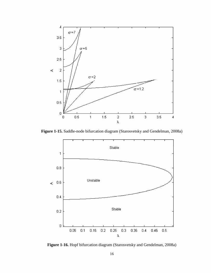
force with amplitude εA. As shown in Figure 1-15, saddle-node bifurcation diagrams are

(1.7)

15

presented in the λ-A plane to show regions of one versus three periodic solutions for

different values of the detuning parameter, σ, while keeping the other parameters fixed.

For each chosen value of σ, regions of one periodic solution are located outside the

curves, while regions of three periodic solutions are bounded inside the curves. Figure 1-

16 shows bifurcation diagrams used again, now in the case of Hopf bifurcations to show

regions of stability and instability. Starosvetsky and Gendelman (2008a) showed also a

method of predicting the occurrence of the Strongly Modulated Response (SMR), which

differs from other methods shown in earlier works. The SMR refers to quasiperiodic

response, that “is characterized by very deep oscillations of the modulated amplitude

comparable to the amplitude of the response itself” (Starosvetsky and Gendelman,

2008a). The response is considered modulated because the “response may be also phase

locked or chaotic”. Finally, numerical simulations are used to validate the results of the

analysis. Notably, Starosvetsky and Gendelman (2008a) showed that two to three

different responses can coexist for the studied system.

Figure 1-14. System considered by Starosvetsky and Gendelman (2008a)

16

Figure 1-15. Saddle-node bifurcation diagram (Starosvetsky and Gendelman, 2008a)

Figure 1-16. Hopf bifurcation diagram (Starosvetsky and Gendelman, 2008a)

17

Starosvetsky and Gendelman (2008b) have presented detailed discussions on the

analysis of the Strongly Modulated Response (SMR) by again considering the system

given by equation (1.7). The SMR “exists in a vicinity of exact 1:1 resonance and is

characterized by relaxation oscillations between stable branches of the slow invariant

manifold” Starosvetsky and Gendelman (2008b). The slow invariant manifold (SIM) is

defined by an equation found through the analysis relating the fixed points of the system,

Φ, to the slow time scale, τ1; in this case,

Φ H Φ |Φ|Φ J .

Note that C(τ1) is simply a consequence of an integration. The relaxation oscillations

refer to jumps from one stable branch to another on the SIM. In order for the SMR to

occur, the system must be essentially nonlinear and possess mass asymmetry. In other

words, the system cannot be reduced to a linear form, and the mass of the attachment

must be much less than the mass of the primary system. Letting the ratio of the mass of

the attachment to the mass of the primary system be denoted by ε, the condition for this

analysis assumes that ε << 1. Beginning with the system given by equation (1.7), the

system equations are manipulated such that they are placed in a form suitable for

studying the SMR, namely, separation into the slow and fast time scales. Phase portraits

are presented for varying amplitudes of the external force, showing how the trajectory

can transition from one stable branch to another. From these phase portraits, a one-

dimensional mapping procedure was discussed. The one-dimensional maps provide a

method of determining regions of existence of the SMR in terms of the detuning

parameter by observation of the existence of attractors on the maps. Since the detuning

parameter is directly related to the natural frequency of the linear system, the conclusion

(1.8)

18

of the SMR existing only near 1:1 resonance was determined in this manner. Further

details on the SMR will be discussed in Chapter 4 of this thesis.

Inclusion of nonlinear damping in a NES attached to a single-degree of freedom

linear system is discussed by Starosvetsky and Gendelman (2009). The system studied,

K , @ A cosL1 ? M

K , @ 0,

regards f as the component possessing the nonlinear damping characteristics. The

nonlinear damping in the system is due to the drag of a fluid through a variable orifice.

See Figure 1-17 for a schematic of the type of device considered. The nonlinearity in the

system is “piecewise-quadratic” since the damping coefficient can be one of two values

depending on the configuration of the flow allowed through the device. The damping

coefficients are denoted by λ1 and λ2, in which λ2 is greater than λ1. Thus, for the system

considered, the damping function is given by

K N | |, | | O PQR | |, | | S PQR T, where acr is a predetermined value inherent in the design of the nonlinear damping

device.

(1.9)

(1.10)

19

Figure 1-17. Schematic of the nonlinear damper (Starosvetsky and Gendelman, 2009)

The main goal of Starosvetsky and Gendelman (2009) was to show that the

inclusion of nonlinear damping in the NES can remove unwanted responses inherent with

a linearly damped NES coupled to a harmonically-forced linear oscillator. Figure 1-18

depicts a linear system coupled to a NES with linear damping. As seen from Figure 1-

18a, an undesired response exists while the SMR (desired) also exists. By increasing the

linear damping coefficient as shown in Figure 1-18b, the undesired response is

eliminated, but the SMR disappears as well. Starosvetsky and Gendelman (2009)

demonstrate in Figure 1-19 how nonlinear damping can resolve this problem. By

choosing certain values for λ1 and λ2, the SMR can exist without the undesired response.

20

Figure 1-18. Linear Damping. (a) λ = 0.2, (b) λ = 1 (Starosvetsky and Gendelman, 2009).

Figure 1-19. Linear versus nonlinear (piecewise-quadratic) damping. (a) λ1 = λ1 = 0.2, (b) λ1 = 0.2 and λ2 = 6 (Starosvetsky and Gendelman, 2009).

(a) (b)

(a) (b)

21

1.3 Comparison of Nonlinear Energy Sinks with Linear Vibration Absorbers

A classical method of reducing vibration in a system is by attaching a linear vibration

absorber, which effectively transfers energy away from the primary system. The simplest

absorber consists of a mass attached to a linear spring, with the spring also attached to the

main system. If designed properly, the vibration energy of the main system is transferred

to the absorber, reducing the vibration in the main system. Ideally, the absorber takes all

of the vibration energy away from the primary system at the fundamental frequency of

the main system, resulting in zero displacement of the main system at this frequency and

very low displacements close to this frequency.

Extending the concept of the vibration absorber to the nonlinear case, a very

powerful method of reducing unwanted vibration is achieved by attaching a nonlinear

energy sink (NES) to the system. A NES is similar to the classical vibration absorber in

that energy is transferred from the primary system to the attachment. However, the NES

can reduce vibrations in the main system at multiple resonant frequencies, as opposed to

the linear vibration absorber which is tuned to operate near a single resonant frequency.

Consequently, the performance of the linear vibration absorber could degrade “over time

due to aging of the system, temperature or humidity variations and so forth, thus

requiring additional adjustment or tuning of parameters” (Lee et al., 2008). Hence, the

degraded linear vibration absorber may become detuned and would operate effectively at

a frequency other than the original if, for example, the spring constant was affected. On

the other hand, if a NES degraded over time in a similar fashion, since there is no

preferred frequency of operation for the NES, the compromise in performance of the NES

would be minimal compared to that of the linear vibration absorber.

22

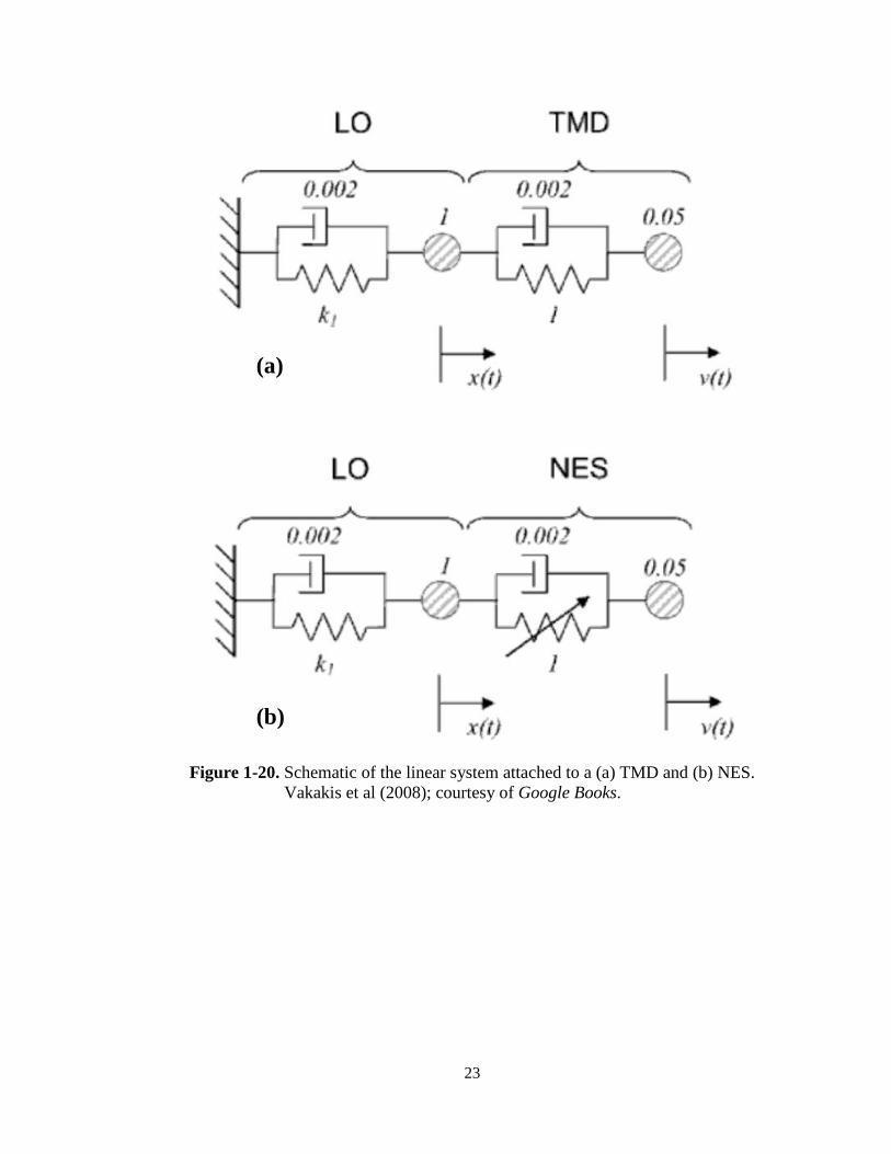
Vakakis et al. (2008) give an example to illustrate some of the benefits of the NES

over classical linear vibration absorbers; in this case, a tuned mass damper (TMD) is

considered. Figure 1-20 shows the two systems considered. In the system with the linear

oscillator (LO) coupled to the TMD, it is clear that the natural frequency of the TMD

alone is √20 rad/s > 4.5 rad/s. Figure 1-21 was generated by varying the stiffness, k1, of

the linear oscillator in each system. In Figure 1-21a, it is evident that the highest

percentage of energy dissipation occurs when the LO natural frequency is approximately

equal to that of the TMD (4.5 rad/s). The energy dissipation drops sharply as the LO

natural frequency deviates from the TMD natural frequency. On the other hand, Figure

1-21b shows that the NES is effective at energy dissipation with a much wider range of

LO natural frequencies compared with the TMD performance. Also notable from Figure

1-21 is that the TMD is independent of, but the NES is heavily reliant on, the impulse

magnitude. Hence, the advantage of having a wide range of frequencies at which the

NES is effective is at the cost of being dependent on the impulse. Chapter 5 of this thesis

presents numerical evidence of the NES dependence on impulse magnitude for a specific

system with nonlinear damping.

23

Figure 1-20. Schematic of the linear system attached to a (a) TMD and (b) NES. Vakakis et al (2008); courtesy of Google Books.

(a)

(b)

24

Figure 1-21. Depiction of energy dissipated as a function of linear natural frequency and impulse magnitude for (a) TMD and (b) NES. Vakakis et al (2008); courtesy of Google Books.

(a)

(b)

25

1.4 Experiments Related to NES

Experiments have been performed to verify the theories of NES. Two requirements for

an NES are that it has “essential (nonlinearizable) stiffness nonlinearities, and that there

exists weak damping dissipation in the integrated linear system-nonlinear attachment

configuration” (Vakakis et al., 2008). As described by (Vakakis et al., 2008), a common

method of achieving nonlinear stiffness in an experimental setup is by using the inherent

nonlinearity in a fixed wire with an applied force at the center corresponding to a

displacement of x. Refer to Figure 1-22 for a depiction of this scenario (Vakakis et al.,

2008). The force,

V3+1 WW 3 /-, is found from the geometry of the wire and location of force application (Vakakis et al.,

2008). Performing a Taylor series expansion of W 3 / about x = 0 gives

W 3 / Y Z[Y\ Z]^Y_ `3a .

Substituting equation (1.12) into equation (1.11) and omitting higher order terms, the

force is expressed with a cubic stiffness relation,

bY[ 3 `3c ,

in which the terms of O(x5) are considered negligible. Caution must be taken in an

experimental setup to ensure very little preload is in the wire while the system is at rest,

as this preload adds a linear stiffness term that makes the stiffness no longer essential (i.e.

the stiffness can be linearized).

Examples of setups for performing experiments relating to NES are discussed by

(Lee et al., 2008) and (Vakakis et al., 2008). One experimental setup, as shown in Figure

(1.11)

(1.12)

(1.13)

26

1-23, involves having the primary system attached to a fixed location with a linear spring,

and the NES is attached to a fixed location with the wire which acts as a nonlinear spring.

Both the linear oscillator and NES are considered grounded in this configuration, and

both masses are connected with a linear spring. The primary system and the NES are

placed on an air track to reduce frictional losses during motion. Another experimental

setup involves taking nearly the same system, but now having the location at which the

ends of the wire are attached move with the NES, thus having an ungrounded NES. This

configuration can simulate a system that is not necessarily confined to one location.

Refer to Figure 1-24 for a depiction of this setup. Figures 1-25 and 1-26 show these two

experimental setups in a schematic form. Since in reality a small amount of damping is

always present, dampers are shown with the linear springs in the diagrams.

Figure 1-22. Depiction of geometry used for stiffness nonlinearity Vakakis et al (2008); courtesy of Google Books.

27

Figure 1-23. Grounded NES in an experimental setup. (a) photograph of setup,

(b) schematic of the setup. Vakakis et al (2008); courtesy of Google Books.

(a)

(b)

28

Figure 1-24. Ungrounded NES in an experimental setup. (a) photograph of setup (b) schematic of the setup, (c) location of NES and LO. Vakakis et al (2008); courtesy of Google Books.

(a)

(b)

(c)

29

Figure 1-25. Primary system and NES attached to fixed locations (grounded system).

Figure 1-26. Primary system attached to fixed location with NES free (ungrounded system).

30

1.5 Outline of this Thesis

The goal of this thesis is to investigate the use of nonlinear damping in a NES attached to

a single degree of freedom linear oscillator. An introduction to the benefits of nonlinear

damping is presented in Chapter 2 with comparisons between the performances of linear,

nonlinear with linear damping (NES), and nonlinear with nonlinear damping one degree

of freedom systems without attachments. Chapter 3 begins the discussions related to the

specific system

1 ? @

@ 0,

quantifying the performance when subjected to harmonic forcing (F= εA cos t). The

strongly modulated response (SMR) is investigated in Chapter 4 through seeking

conditions for the existence of this response. Chapter 5 compares the performance of the

same system subjected now to impulsive loading of different amplitudes with a similar

system having linear damping. Additionally, phase portraits and Poincaré maps are

shown in Chapter 5 to further examine the performance of the linearly and nonlinearly

damped systems subjected to harmonic excitations. Conclusions and recommendations

are presented in Chapter 6.

1.6 Summary

This chapter has presented a brief overview of the concepts of nonlinear energy sinks

(NES), targeted energy transfer (TET), and resonance capture (RC), which are essential

to the understanding of the mitigation of vibration using a special class of nonlinear

absorbers. Pertinent contributions to the theoretical and experimental behavior of this

(1.14)

31

class of nonlinear absorbers are presented. Also, the relationship of such contributions to

the scope of this thesis is outlined.

32

2.0 Concept Energy Sinks with Nonlinear Stiffness and Damping

2.1 Introduction

Substantial benefits regarding vibration mitigation can be achieved by including

nonlinear components in a system. Since nonlinear springs and nonlinear viscous

dampers can have forces proportional to any exponential power of displacement and

velocity, respectively, greater flexibility in system design is allowed with their inclusion.

This section presents simple examples to illustrate the advantages of having nonlinear

components in systems.

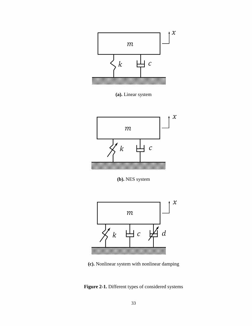
2.2 Description of Considered Systems

Three systems are compared in this section in order to illustrate the advantages of

nonlinear stiffness and nonlinear damping characteristics in terms of vibration mitigation.

The three systems under consideration are: a linear system, a NES system, and a

nonlinear system with nonlinear damping. For simplicity, only one degree of freedom

systems are considered. The linear system consists of a mass attached to a linear spring

and a linear damper as shown in Figure 2-1a. The NES system replaces the linear spring

with a nonlinear spring having restoring force proportional to the cube of displacement as

shown in Figure 2-1b. Finally, the nonlinear system with nonlinear damping expands on

the NES system by including a nonlinear damper having a damping force proportional to

the velocity cubed as shown in Figure 2-1c.

33

(a). Linear system

(b). NES system

(c). Nonlinear system with nonlinear damping

Figure 2-1. Different types of considered systems

34

2.3 Analysis of the Different Systems

2.3.1 Linear System

The equation of motion is written as

d3 e3 V3 0.

In order to perform the numerical integration, the equation of motion is cast into the

following state space form:

N33 f g 0 1 bh Qhi j33k,

where

3 3 and 3 3 . The system total energy is given by

l d3 V3.

Taking the derivative of the energy equation with respect to time gives the rate of energy

decay,

l d3 V3 3 e3 O 0.

2.3.2 NES System


d3 e3 V3 0.



N33 f g 0 1 bZm[h Qhi j33k,

(2.1)

(2.2)

(2.3)

(2.4)

(2.5)

(2.6)

(2.7)

35

where


l d3 @ V3@.


decay,

l d3 V3 3 e3 O 0.

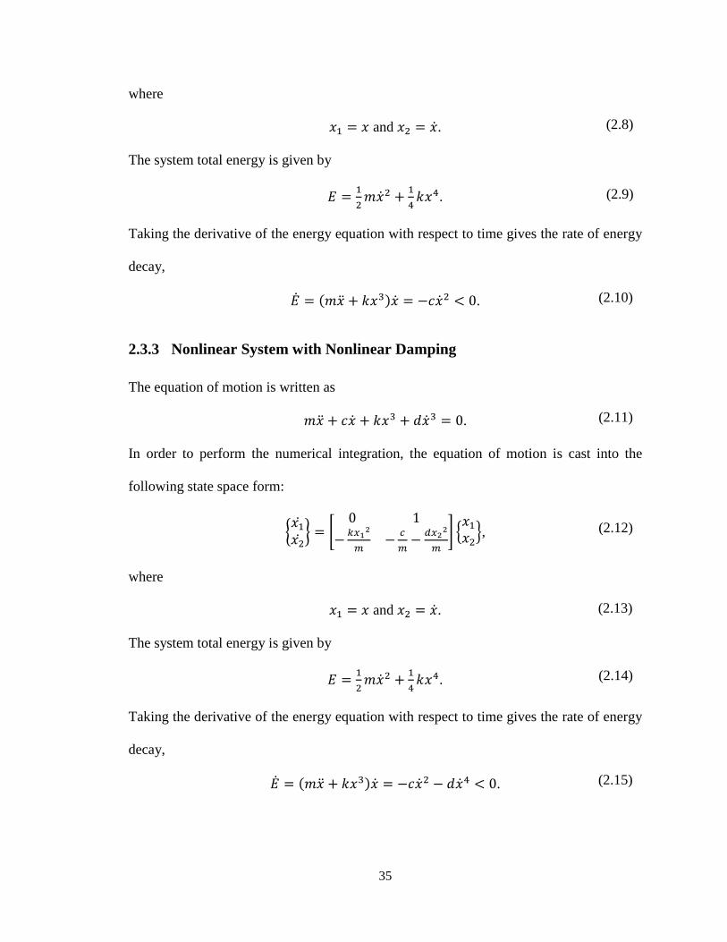
2.3.3 Nonlinear System with Nonlinear Damping


d3 e3 V3 3 0.



N33 f g 0 1 bZm[h Qh nZ[[h i j33k,

where


l d3 @ V3@.


decay,

l d3 V3 3 e3 3 @ O 0.

(2.10)

(2.8)

(2.9)

(2.11)

(2.12)

(2.13)

(2.14)

(2.15)

36

2.4 Performance Comparisons

For comparison between the performances of each system, the equations of motion,

equations of the total system energy, and equations of system energy decay were

generated for all three cases. The equations of motion,

W;oPp d3 e3 V3 0 (2.16a)

qlr d3 e3 V3 0 (2.16b)

qs;t;oPp uv ;s;t;oPp Pd#;w d3 e3 V3 3 0, (2.16c)

were used to determine displacement as a function of time. The Runge-Kutta 4

numerical method was used to solve these equations. Parameters were chosen for a

lightly damped (ζ = 0.075) linear system as shown in Table 2-1.

Table 2-1. System Parameters for Numerical Solutions

System m k c d

Linear 1 4 0.3 0

NES 1 4 0.3 0

Nonlinear with nonlinear damping 1 4 0.3 2

In performing the analysis, each system was initially at rest and given an initial

displacement of 1. As shown in Figure 2-2, the frequency of oscillation of each system is

different. The linear system has a faster oscillation frequency than the NES system, and

the nonlinear system with nonlinear damping has the slowest oscillation frequency. The

37

displacement of the nonlinear system with nonlinear damping appears to have smoother

transitions from peak to peak, and the amplitude of the displacement is reduced faster

than that for the linear and NES systems.

Further comparisons between the performances of each system can be made by

observing the total system energy as a function of time. The total system energy is

governed by

W;oPp l 12 d3 12 V3 (2.17a)

qlr l 12 d3 14 V3@ (2.17b)

qs;t;oPp uv ;s;t;oPp Pd#;w l 12 d3 14 V3@. (2.17c)

By plotting the total energy for each system versus time, Figure 2-3 was obtained.

Initially, the linear system has twice as much energy as the other two systems. Since the

initial velocity is zero, the greater initial system energy is a consequence of the potential

energy term in the equations. Observing the graphs, it is clear that the nonlinear system

with nonlinear damping decays faster than both the NES and linear systems.

By taking the derivative with respect to time of the energy equations, the

equations representing energy decay,

W;oPp l d3 V3 3 e3 (2.18a)

qlr l d3 V3 3 e3 (2.18b)

qs;t;oPp uv ;s;t;oPp Pd#;w l d3 V3 3 e3 3 @, (2.18c)

are determined. Figure 2-4 shows the magnitude of energy decay for each system as a

function of time. The linear system evidently takes the longest time to finish dissipating

the system energy. The NES system energy decay is faster than that of the linear system.

38

Although the first peak of energy decay on the NES system plot is lower than that of the

linear system, the slower period of energy decay in the NES system allows energy to be

dissipated more rapidly. In contrast to the linear and NES systems, the plot of energy

decay for the nonlinear system with nonlinear damping shows a relatively high peak

followed by a rapid decrease in energy decay. Due to the large initial energy decay, the

system energy is dissipated much more quickly than the other two systems. Thus, the

nonlinear system with nonlinear damping is more effective at energy dissipation than the

linear or NES systems.

Figure 2-2. Time response of each system

0 5 10 15 20 25 30 35-1

0

1Linear System

Dis

pla

cem

ent,

x

0 5 10 15 20 25 30 35-1

0

1NES System

Dis

pla

cem

ent,

x

0 5 10 15 20 25 30 35-1

0

1Nonlinear System with Nonlinear Damping

Time, t

Dis

pla

cem

ent,

x

39

Figure 2-3. System Energy versus time for each system

Figure 2-4. Magnitude of energy decay versus time for each system

0 5 10 15 20 25 30 350

1

2Linear System

Sys

tem

En

erg

y, E

0 5 10 15 20 25 30 350

1

2NES System

Sys

tem

En

erg

y, E

0 5 10 15 20 25 30 350

1


Time, t

Sys

tem

En

erg

y, E

0 5 10 15 20 25 30 350

1

2Linear System

|E D

ecay

|, |d

E/d

t|

0 5 10 15 20 25 30 350

1

2NES System

|E D

ecay

|, |d

E/d

t|

0 5 10 15 20 25 30 350

1


Time, t

|E D

ecay

|, |d

E/d

t|

40

The results presented in this section have shown that the nonlinear system with

nonlinear damping can be far more effective at mitigating vibration than the linear or

NES counterparts. The motion of the nonlinear system with nonlinear damping comes to

rest more quickly than the other two systems. The rapid reduction in system

displacement is due to the system energy being dissipated faster in the nonlinear system

with nonlinear damping than in the NES or linear systems. Including nonlinear damping

in the system clearly can have a dramatic influence on the system performance. Since the

nonlinear damping term is a function of velocity cubed, this term is much more effective

at dissipating system energy than a linear damping term.

2.5 Summary

As evident from the examples presented in this section, systems possessing nonlinear

damping characteristics can vastly outperform their linear counterparts. In designing a

system, the coefficient of the nonlinear damping term could be chosen to reduce system

energy much more quickly than a system with only linear damping. Practically,

including nonlinear terms allows the designer more options when designing a system.

41

2.A Appendix

In MATLAB, the Runge-Kutta 4 method was used to numerically integrate the equations

of motion, equations of system energy, and equations of energy decay. For ease of

explanation, the magnitude of energy decay was determined. Note that the energy decay

is always negative; thus the magnitude of energy decay is equal to the energy decay

multiplied by -1. The following code was used to generate the plots shown in Figure 2-2,

Figure 2-3, and Figure 2-4.

%Numerical Comparison of NES, Linear, and Nonlinear with Nonlinear %Damping Systems close all clear all T = 0.001; h = 1; c = .3; k = 4; m = 1; d = 2; t_end = 35; %end of time interval x10 = 1; %initial displacement x20 = 0; %initial velocity t_vec = zeros(1,t_end/T + 1); x1_NES_vec = t_vec; x2_NES_vec = t_vec; x1_Lin_vec = t_vec; x2_Lin_vec = t_vec; x1_NonL_vec = t_vec; x2_NonL_vec = t_vec; E_NES_vec = t_vec; E_dot_NES_vec = t_vec; E_Lin_vec = t_vec; E_dot_Lin_vec = t_vec; E_NonL_vec = t_vec; E_dot_NonL_vec = t_vec; x1_NES = x10; x1_NES_vec(1) = x10; x2_NES = x20; x2 _NES_vec(1) = x20; x1_Lin = x10; x1_Lin_vec(1) = x10; x2_Lin = x20; x2 _Lin_vec(1) = x20; x1_NonL = x10; x1_NonL_vec(1) = x10; x2_NonL = x20; x2_NonL_vec(1) = x20; E_NES_vec(1) = 1/2*m*x2_NES^2 + 1/4*k*x1_NES^4; E_dot_NES_vec(1) = c*x2_NES^2; E_Lin_vec(1) = 1/2*m*x2_Lin^2 + 1/2*k*x1_Lin^2; E_dot_Lin_vec(1) = c*x2_Lin^2; E_NonL_vec(1) = 1/2*m*x2_NonL^2 + 1/4*k*x1_NonL^4; E_dot_NonL_vec(1) = c*x2_NonL^2; %Runge Kutta 4 %From Fundamentals of Vibrations by Leonard Meirovi tch, p. 677-679: for t = T:T:t_end h = h+1; t_vec(h) = t;

42

%NES System: f11 = x2_NES; f12 = -(c*x2_NES + k*x1_NES^3)/m; g11 = T*f11; g12 = T*f12; f21 = x2_NES + 1/2*g12; f22 = -(c*(x2_NES+1/2*g 12) + ... k*(x1_NES+1/2*g11)^3)/m; g21 = T*f21; g22 = T*f22; f31 = x2_NES + 1/2*g22; f32 = -(c*(x2_NES+1/2*g 22) + ... k*(x1_NES+1/2*g21)^3)/m; g31 = T*f31; g32 = T*f32; f41 = x2_NES + g32; f42 = -(c*(x2_NES+g32) + k* (x1_NES+g31)^3)/m; g41 = T*f41; g42 = T*f42; x1_NES = x1_NES + 1/6*(g11 + 2*g21 + 2*g31 + g4 1); x2_NES = x2_NES + 1/6*(g12 + 2*g22 + 2*g32 + g4 2); E_NES = 1/2*m*x2_NES^2 + 1/4*k*x1_NES^4; E_dot_NES = c*x2_NES^2; x1_NES_vec(h) = x1_NES; x2_NES_vec(h) = x2_NES; E_NES_vec(h) = E_NES; E_dot_NES_vec(h) = E_dot_ NES; %Linear System: f11 = x2_Lin; f12 = -(c*x2_Lin + k*x1_Lin)/m; g11 = T*f11; g12 = T*f12; f21 = x2_Lin + 1/2*g12; f22 = -(c*(x2_Lin+1/2*g 12) + ... k*(x1_Lin+1/2*g11))/m; g21 = T*f21; g22 = T*f22; f31 = x2_Lin + 1/2*g22; f32 = -(c*(x2_Lin+1/2*g 22) + ... k*(x1_Lin+1/2*g21))/m; g31 = T*f31; g32 = T*f32; f41 = x2_Lin + g32; f42 = -(c*(x2_Lin+g32) + k* (x1_Lin+g31))/m; g41 = T*f41; g42 = T*f42; x1_Lin = x1_Lin + 1/6*(g11 + 2*g21 + 2*g31 + g4 1); x2_Lin = x2_Lin + 1/6*(g12 + 2*g22 + 2*g32 + g4 2); E_Lin = 1/2*m*x2_Lin^2 + 1/2*k*x1_Lin^2; E_dot_Lin = c*x2_Lin^2; x1_Lin_vec(h) = x1_Lin; x2_Lin_vec(h) = x2_Lin; E_Lin_vec(h) = E_Lin; E_dot_Lin_vec(h) = E_dot_ Lin; %Nonlinear System: f11 = x2_NonL; f12 = -(c*x2_NonL + k*x1_NonL^3 + d*x2_NonL^3)/m; g11 = T*f11; g12 = T*f12; f21 = x2_NonL + 1/2*g12; f22 = -(c*(x2_NonL+1/2 *g12) + ...

43

k*(x1_NonL+1/2*g11)^3 + d*(x2_NonL+1/2*g12) ^3)/m; g21 = T*f21; g22 = T*f22; f31 = x2_NonL + 1/2*g22; f32 = -(c*(x2_NonL+1/2 *g22) + ... k*(x1_NonL+1/2*g21)^3 + d*(x2_NonL+1/2*g22) ^3)/m; g31 = T*f31; g32 = T*f32; f41 = x2_NonL + g32; f42 = -(c*(x2_NonL+g32) + ... k*(x1_NonL+g31)^3 + d*(x2_NonL+g32)^3)/m; g41 = T*f41; g42 = T*f42; x1_NonL = x1_NonL + 1/6*(g11 + 2*g21 + 2*g31 + g41); x2_NonL = x2_NonL + 1/6*(g12 + 2*g22 + 2*g32 + g42); E_NonL = 1/2*m*x2_NonL^2 + 1/4*k*x1_NonL^4; E_dot_NonL = c*x2_NonL^2 + d*x2_NonL^4; x1_NonL_vec(h) = x1_NonL; x2_NonL_vec(h) = x2_N onL; E_NonL_vec(h) = E_NonL; E_dot_NonL_vec(h) = E_d ot_NonL; end figure subplot(3,1,1); plot(t_vec, x1_Lin_vec, '-k' , 'LineWidth' , 2); grid on; title( '\bfLinear System' ); ylabel( '\bfDisplacement, \itx' ); subplot(3,1,2); plot(t_vec, x1_NES_vec, '-k' , 'LineWidth' , 2); grid on; title( '\bfNES System' ); ylabel( '\bfDisplacement, \itx' ); subplot(3,1,3); plot(t_vec, x1_NonL_vec, '-k' , 'LineWidth' , 2); grid on; title( '\bfNonlinear System with Nonlinear Damping' ) xlabel( '\bfTime, \itt' ); ylabel( '\bfDisplacement, \itx' ); figure subplot(3,1,1); plot(t_vec, E_Lin_vec, '-k' , 'LineWidth' , 2); grid on; title( '\bfLinear System' ); ylabel( '\bfSystem Energy, \itE' ); subplot(3,1,2); plot(t_vec, E_NES_vec, '-k' , 'LineWidth' , 2); grid on; title( '\bfNES System' ); ylabel( '\bfSystem Energy, \itE' ); axis([0 t_end 0 2]); subplot(3,1,3); plot(t_vec, E_NonL_vec, '-k' , 'LineWidth' , 2); grid on; title( '\bfNonlinear System with Nonlinear Damping' ) xlabel( '\bfTime, \itt' ); ylabel( '\bfSystem Energy, \itE' ); axis([0 t_end 0 2]); figure subplot(3,1,1); plot(t_vec, E_dot_Lin_vec, '-k' , 'LineWidth' , 2); grid on; title( '\bfLinear System' ); ylabel( '\bf|E Decay|, \it|dE/dt|' ); axis([0 t_end 0 2]); subplot(3,1,2); plot(t_vec, E_dot_NES_vec, '-k' , 'LineWidth' , 2); grid on; title( '\bfNES System' ); ylabel( '\bf|E Decay|, \it|dE/dt|' ); axis([0 t_end 0 2]); subplot(3,1,3); plot(t_vec, E_dot_NonL_vec, '-k' , 'LineWidth' , 2); grid on; title( '\bfNonlinear System with Nonlinear Damping' ) xlabel( '\bfTime, \itt' ); ylabel( '\bf|E Decay|, \it|dE/dt|' );

44

3.0 Nonlinear Analysis of Nonlinear Energy Sinks

3.1 Introduction

This section analyzes the performance of a selected system, which is a modification of

the system studied in “Response regimes of linear oscillator coupled to nonlinear energy

sink with harmonic forcing and frequency detuning” by Starosvetsky and Gendelman

(2008). Starosvetsky and Gendelman (2008) considered a linear system with an

attachment consisting of linear damping and cubic nonlinear stiffness. This thesis

extends the work to the case of the linear system with the attachment now having cubic

nonlinear damping. Physically, the system under consideration in both cases corresponds

to a harmonically forced linear structure with a strongly nonlinear attachment acting as a

nonlinear energy sink (NES). The equations of motion of the system under consideration

are given by

1 ? @ A cos

@ 0,

where y1 is the displacement of the linear oscillator, y2 is the displacement of the

attachment, ελ is the damping coefficient, εA is the amplitude of external force, and εσ is

the frequency detuning parameter. From equations (3.1), it is evident that the

nonlinearities appear in both equations as the cube of difference in velocity and

difference in displacement between the linear system and the NES. For simplicity in this

chapter of the thesis, the terms “damping coefficient”, “amplitude of external force”, and

“frequency detuning parameter” refer to the same parameters as Starosvetsky and

Gendelman (2008), without the coefficient, ε.

(3.1)

45

In this thesis, periodic solutions are described in Section 3.2 and Section 3.3 with

the use of saddle-node and Hopf bifurcations, respectively. Finally, conclusions are

discussed at the end of this chapter.

3.2 Saddle-Node Bifurcation

3.2.1 Saddle-Node Bifurcation Background

The goal of this section is to describe the periodic solutions of the system through

examining the saddle-node bifurcations. A bifurcation represents “a qualitative change in

the features of a system, such as the number and type of solutions,” due to “the variation

of one or more parameters on which the considered system depends” (Nayfeh and

Balachandran, 1995). By looking at a plot of system parameters (displacement versus a

scalar parameter, for example), one can often decipher the type of bifurcation by visual

inspection. In order to study bifurcations, the system is frequently put in the form

x yx; ,

in which x is the state vector and x is the derivative of x with respect to time. On the

right hand side of (3.2), F is called the vector field and is a function of x and µ, a scalar

parameter (Nayfeh and Balachandran, 1995).

For a saddle-node bifurcation to exist, F must equal the zero vector, and the

Jacobian of F (denoted by DxF) must have at least one zero eigenvalue and the remaining

eigenvalues having nonzero real parts (Nayfeh and Balachandran, 1995). The first of

these prerequisites is the condition for a fixed point to exist. At the fixed point, x equals

the zero vector, and x can be superficially replaced with x0 in order to represent the fixed

(3.2) (3.2)

46

point. In addition to the aforementioned two criteria for a saddle-node bifurcation, one

final condition must be met. Let

y| 8y8,

with F being an n x 1 vector, thus DxF is an n x n vector. For a saddle-node bifurcation

to occur, the n x (n + 1) matrix [DxF | Fµ] must be of rank n (Nayfeh and Balachandran,

1995).

A simple example of a saddle-node bifurcation (given by Nayfeh and

Balachandran, 1995) involves the system

3 3,

where µ is a scalar control parameter. By setting 3 equal to zero and solving for x, the

fixed points of the system,

3 ~√,

are obtained. Figure 3-1 shows a plot of x versus µ, with a saddle-node bifurcation

occurring at the origin. This bifurcation is a saddle-node because the three conditions are

satisfied for this system. The first condition (F must equal the zero vector) is satisfied by

setting 3 equal to zero since 3 . Taking the Jacobian of F gives

/Z 88Z 23,

and at x = 0, DxF = 0. Setting

/Z 0

gives the eigenvalue λ = 0. Thus, this system has a zero eigenvalue at the bifurcation

point. Finally, solving for

y| 8y8 1,

(3.3)

(3.4)

(3.5)

(3.6)

(3.7)

(3.8)

47

the matrix [DxF | Fµ] becomes [0 1] at the point x = 0, µ = 0. Since this matrix has only

one linearly independent column, the rank of the matrix is one. The bifurcation is a

saddle node bifurcation because all three conditions have been satisfied.

The plot in Figure 3-1 consists of two branches, each corresponding to one of the

fixed points. In general, saddle-node bifurcations are characterized by two branches

terminating at a single point, the bifurcation point. Note that the qualitative change in

Figure 3-1 occurs at the location where the stable branch meets the unstable branch. At

the origin, there is a single fixed point solution. However, at values of µ > 0, there are

two solutions; thus we have a qualitative change in the system. Stability will be

discussed in Section 3.3 with the study of Hopf bifurcations, as this knowledge is not

necessary for understanding the saddle-node bifurcation impact on number of solutions.

Figure 3-1. Saddle-node bifurcation given by equation (3.4)

-2 -1.5 -1 -0.5 0 0.5 1 1.5 2-2

-1.5

-1

-0.5

0

0.5

1

1.5

2

µµµµ

x

stableunstable

48

3.2.2 Saddle-Node Bifurcation Analysis for the Linearly Damped System

Armed with a general understanding of saddle-node bifurcations, the focus of this section

is shifted to the system with linear damping given by

1 ? @ A cos

@ 0.

The following derivations are based on the work done by Starosvetsky and Gendelman

(2008). By making a change of variables according to

5 , u ,

o 5 5, o u u,

and omitting exponential terms from the resulting set of equations, we can rewrite the

system as

and

H 1 || .

Setting the time derivatives of equation (3.11) to zero gives

4 4 4 4 ,

and

H 4 4 4 4 4

1 |4|4 ,

where φ10 and φ20 are the fixed points of the system. The equations (3.12) lead to

4 [

(3.9)

(3.10)

(3.12)

(3.13)

(3.11)

49

and

[ [ |4| |4|@ |4|a [ [.

As a simplification, equation (3.14) can be rewritten as

@ 0,

where

|4| , [ [

, 1, @ [ [.

Taking the derivative of equation (3.15) with respect to Z gives

3 2 0.

Eliminating Z from equations (3.15) and (3.17) as shown in Section 3.A.1 gives

@ [\ ~ [[m\\ [\ ~ [[m\\ [\ ~ [[m\\ .

The expression given in equation (3.18) represents the boundary of the saddle-node

bifurcation, which separates regions of one periodic solution from regions of three

periodic solutions. From equation (3.18), Figure 3-2, Figure 3-3, and Figure 3-4 were

generated. The boundary can be checked by substituting values for λ and A into

equations (3.16) and (3.18), then determining the number of real periodic solutions. For

example, from Figure 3-2, choosing λ = 0.3 and A = 1 falls within the region of three real

periodic solutions. However, for λ = 0.3 and A = 0.2, there is only one real periodic

solution.

(3.14)

(3.15)

(3.16)

(3.17)

(3.18)

50

Figure 3-2. Saddle-node bifurcation for σ = 3 (linear damping)

Figure 3-3. Saddle-node bifurcations for positive values of σ (linear damping)

0 0.1 0.2 0.3 0.4 0.5 0.6 0.7 0.8 0.9 10

0.5

1

1.5

2

2.5

λλλλ

A

λλλλ = 0.3, A = 0.2Z1 = 1.4979-0.28908iZ2 = 1.4979+0.28908iZ3 = 0.0042971

λλλλ = 0.3, A = 1Z1 = 1.7329Z2 = 1.1406Z3 = 0.12648

λλλλ = 0.3, A = 1.7Z1 = 2.0178Z2 = 0.49112-0.34186iZ3 = 0.49112+0.34186i

0 0.5 1 1.5 2 2.5 3 3.50

0.5

1

1.5

2

2.5

3

3.5

4

4.5

λλλλ

A

σσσσ = 1.2σσσσ = 2

σσσσ = 5

σσσσ = 7

51

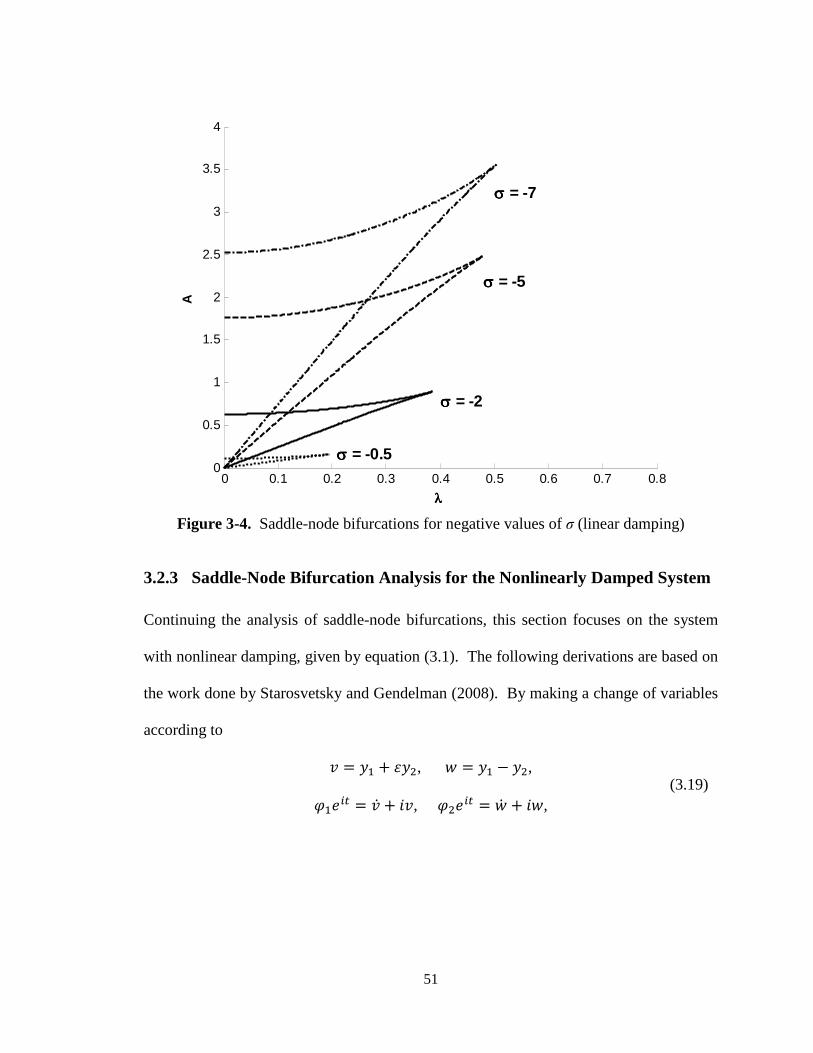
Figure 3-4. Saddle-node bifurcations for negative values of σ (linear damping)

3.2.3 Saddle-Node Bifurcation Analysis for the Nonlinearly Damped System

Continuing the analysis of saddle-node bifurcations, this section focuses on the system

with nonlinear damping, given by equation (3.1). The following derivations are based on

the work done by Starosvetsky and Gendelman (2008). By making a change of variables

according to

5 , u ,

o 5 5, o u u,

0 0.1 0.2 0.3 0.4 0.5 0.6 0.7 0.80

0.5

1

1.5

2

2.5

3

3.5

4

λλλλ

A

σσσσ = -0.5

σσσσ = -2

σσσσ = -5

σσσσ = -7

(3.19)

52

and omitting exponential terms from the resulting set of equations, we can rewrite the

system as

and

1 || 1 || .

Setting the time derivatives of equation (3.20) to zero gives

4 4 4 4 ,

and

1 |4|4 4 4 4 4

1 |4|4 ,

where φ10 and φ20 are the fixed points of the system. The equations (3.21) lead to

4 [

and

[ [ |4| |4|@ a 1 |4|a [ [. As a simplification, equation (3.23) can be rewritten as

@ 0,

where

|4| , [ [

, a 1, @ [ [.


3 2 0.

(3.20)

(3.21)

(3.22)

(3.23)

(3.24)

(3.25)

(3.26)

53

Eliminating Z from equations (3.24) and (3.26) as shown in Section 3.A.2 gives

@ [\ ~ [[m\\ [\ ~ [[m\\ [\ ~ [[m\\ .

The expression given in equation (3.27) represents the boundary of the saddle-node

bifurcation, which separates regions of one periodic solution from regions of three

periodic solutions. From equation (3.27), Figure 3-5, Figure 3-6, and Figure 3-7 were

generated. The boundary can be checked by substituting values for λ and A into

equations (3.15) and (3.27), then determining the number of real periodic solutions. For

example, from Figure 3-5, choosing λ = 0.3 and A = 1 falls within the region of three real

periodic solutions. However, for λ = 0.3 and A = 0.2, there is only one real periodic

solution.

Figure 3-5. Saddle-node bifurcation for σ = 3 (nonlinear damping)

0 0.1 0.2 0.3 0.4 0.5 0.6 0.7 0.8 0.9 10

0.5

1

1.5

2

2.5

λλλλ

A

λλλλ = 0.3, A = 0.2Z1 = 1.4255-0.31117iZ2 = 1.4255+0.31117iZ3 = 0.0044711

λλλλ = 0.3, A = 1Z1 = 1.6338Z2 = 1.0878Z3 = 0.13389

λλλλ = 0.3, A = 1.7Z1 = 1.9307Z2 = 0.46237-0.37736iZ3 = 0.46237+0.37736i

(3.27)

54

Figure 3-6. Saddle-node bifurcations for positive values of σ (nonlinear damping)

Figure 3-7. Saddle-node bifurcations for negative values of σ (nonlinear damping)

0 0.5 1 1.5 2 2.5 3 3.50

0.5

1

1.5

2

2.5

3

3.5

4

4.5

λλλλ

A

σσσσ = 1.2

σσσσ = 2

σσσσ = 5

σσσσ = 7

0 0.1 0.2 0.3 0.4 0.5 0.6 0.7 0.80

0.5

1

1.5

2

2.5

3

3.5

4

λλλλ

A

σσσσ = -0.5

σσσσ = -2

σσσσ = -5

σσσσ = -7

55

3.2.4 Discussion of Results for Saddle-Node Bifurcations

From inspection of Figures 3-2 through 3-7, it is evident that the saddle-node bifurcations

all have the same shape for the various chosen values for σ. Additionally, by observation

of the saddle-node bifurcation diagrams, the value of A for the fixed points increases as

the magnitude of σ increases.

In Figures 3-2 and 3-5, the solutions are shown at three different points as

a spot-check of the different regions. For any λ and A within the region bounded by the

two curves, all three periodic solutions are real. However, for all λ and A outside of this

region, only one of the three periodic solutions is real, and the other two have imaginary

components. Figures 3-3, 3-4, 3-6, and 3-7 represent the same scenario of real periodic

solutions for varying values of σ.

Comparing the boundary of the saddle-node bifurcation for the linearly

damped system (Figure 3-2) with that for the nonlinearly damped system (Figure 3-5),

there has been a clearly visible qualitative change. For both systems, each branch starts

off at approximately the same initial value for λ = 0. The upper branch of the linearly

damped system shows a more well-defined concave shape as opposed to the upper branch

of the nonlinearly damped system. Conversely, the lower branch of the linearly damped

system appears more linear than the curved shape of the lower branch of the nonlinearly

damped system. Lastly, it can be seen that the two branches converge for a lower value

of λ for the nonlinearly damped system than for the linearly damped system. The same

qualitative trend is apparent for different values of sigma, as depicted in Figures 3-3, 3-4,

3-6, and 3-7. These plots show that with an increasing magnitude of σ, there is an

56

increasing trend in the amplitude, A. However, there is one exception to this trend, since

in the nonlinearly damped system the amplitude for σ = 1.2 is greater than that for σ = 2.

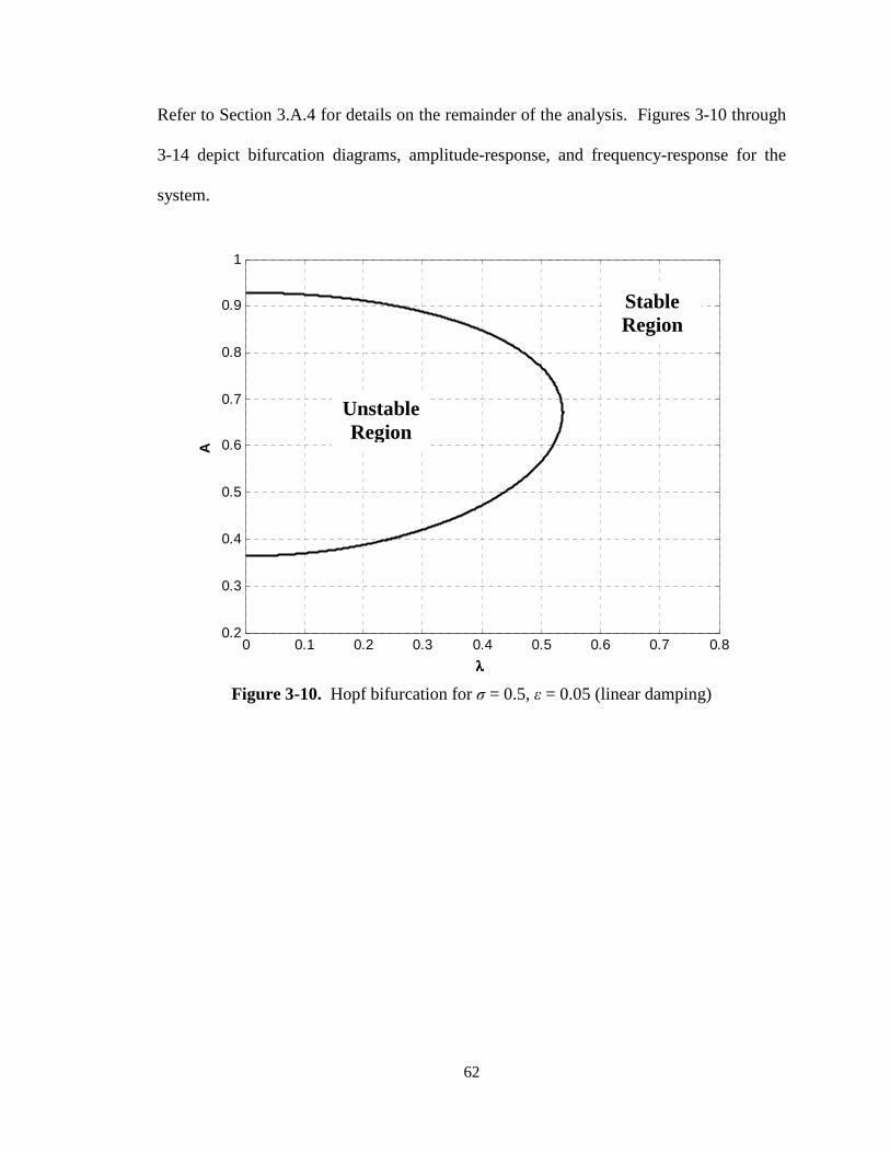
3.3 Hopf Bifurcation

3.3.1 Hopf Bifurcation Background

The purpose of studying Hopf bifurcations in the context of this thesis is to determine

regions of stability of the periodic solutions. Similar to saddle-node bifurcations, Hopf

bifurcations represent a qualitative change in the system. For a Hopf bifurcation to exist,

the vector field F, given in equation (3.2), must equal the zero vector. When the vector

field F is equal to the zero vector, let x = x0 and µ = µc. Hence, another necessary

criterion for a Hopf bifurcation is that the Jacobian of F (denoted by DxF) must have at

least one “pair of purely imaginary eigenvalues, while all of its other eigenvalues have

nonzero real parts at” (x0; µc) (Nayfeh and Balachandran, 1995). The final condition for a

Hopf bifurcation is that the derivative of the real part of the eigenvalues with respect to µ

does not equal zero at µc.

An example of a Hopf bifurcation was presented by Nayfeh and Balachandran

(1995). With the scalar control parameter µ, the following system is considered:

3 3 3 3

3 3 3 .

The system given in equation (3.28) can be written in the form

N3 f y3, ; ,

(3.28)

(3.29)

57

where the vector F represents the right hand side of equation (3.28). Taking the Jacobian

of F from equation (3.29) gives

/Zy 8 8Z 8 8Z8 8Z 8 8Z 8Z8Z 8Z888Z 88. Thus,

/Zy 33 23 3 23 3 33 23 3 23 3 . From inspection of equation (3.28), it is obvious that (0,0) is a fixed point because at this

condition 3 0 and 0. For this fixed point, the Jacobian reduces to

/Zy . The eigenvalues are found by taking the determinant of DxF – λ[I] and setting the

expression equal to zero. Thus,

0.

Taking the determinant in equation (3.33) and solving the characteristic equation for λ

gives the eigenvalues

, ~ .

As shown by Nayfeh and Balachandran (1995), the condition for the derivative of the

eigenvalues with respect to µ not being equal to zero is satisfied since

nHmn 1 and nH[n 1.

For a Hopf bifurcation to occur, the eigenvalues must be purely imaginary. Thus, letting

µ = 0, the eigenvalues become

9! , ~.

(3.30)

(3.31)

(3.32)

(3.33)

(3.34)

(3.35)

(3.36)

58

In order to create the bifurcation diagrams, first equations (3.28) are converted to polar

form using the relations

3 p cos and p sin .

The system equations then become

p p p

p.

Fixed points are determined by setting the time derivatives in equation (3.38) equal to

zero. Solutions for the trivial and nontrivial fixed points are

p 0 and p ~ ,

respectively. The Jacobian is found from

/Zy 88R 8R8R 3p.

The eigenvalues are determined by setting DxF – λ[I] equal to zero and solving for λ.

Thus,

3p.

For the trivial fixed point, equation (3.41) reduces to

R4 ,

and for the nontrivial fixed points, equation (3.41) becomes

==R 2.

The corresponding bifurcation diagrams for the fixed points from equation (3.39) are

presented in Figure 3-8 for α = -1 and Figure 3-9 for α = 1.

From inspection of Figures 3-8 and 3-9, the Hopf bifurcation occurs as predicted

at µ = 0. At this point, there is a qualitative change in the system, namely, the number of

(3.38)

(3.39)

(3.40)

(3.41)

(3.42)

(3.43)

(3.37)

59

solutions and stability. For α = -1 as shown in Figure 3-8, any given negative value of µ

results in one stable solution, while any given positive value of µ results in two stable

solutions and one unstable solution. Note that stability was assessed by the sign of the

real part of the eigenvalues, based on equation (3.42) for the trivial fixed point and

equation (3.43) for the nontrivial fixed points. Negative real parts result in stable

solutions, and positive real parts result in unstable solutions. A similar, but different,

scenario from Figure 3-8 is depicted in Figure 3-9 for α = 1. In this case, a positive value

of µ results in a single unstable solution, but negative values of µ result in two unstable

solutions and one stable solution.

Figure 3-8. Bifurcation diagram of system (3.28) in polar form for α = -1. = stable; = unstable

-2 -1.5 -1 -0.5 0 0.5 1 1.5 2-1.5

-1

-0.5

0

0.5

1

1.5

µµµµ

r

60

Figure 3-9. Bifurcation diagram of system (3.28) in polar form for α = 1. = stable; = unstable

3.3.2 Hopf Bifurcation Analysis for the System with Linear Damping

For the dynamical system given by equation (3.9), let

4 , 4 ,

and substituting into equations (3.11) while omitting the nonlinear terms gives

,

¡ ¡ ¡ ¡ ¡ ,

H

1 |4| 4¡, ¡ H ¡ ¡ ¡ ¡ ¡

1 |4|¡ 4¡ .

-2 -1.5 -1 -0.5 0 0.5 1 1.5 2-1.5

-1

-0.5

0

0.5

1

1.5

µµµµ

r

(3.44)

(3.45)

61

The characteristic polynomial can be written as

@ ¢ ¢ ¢ ¢@ 0,

where µ are the eigenvalues, and

|4| q4, q4@ 44¡ ,

¢ 1 ,

¢ 32 34 34 q4@ ? 1 q4 14 1 14 ? 1 , ¢ @ ? 1 ,

¢@ a 1 ? q4@ @ ?1 ? q4 a 1 ? ?£. For the Hopf bifurcation to occur, we must have

~Ω,

in which Ω is a real number. Substituting equation (3.48) into equation (3.46) and

separating into real and imaginary parts gives

Ω@ ¢Ω ¢@ 0, Ω¢Ω ¢ 0 ¥ Ω ¦\¦m.

Substituting the relation for Ω2 into the first equation of equation (3.49) gives

¢ ¢¢¢ ¢@¢ 0.

MATLAB was used to determine the coefficients, vi, for

5§ 5§ 5 0,

based on equation (3.50). Solving for z in equation (3.51) gives

§, [¨[[@\mm ,

and from equation (3.15), the boundaries of stability are given by

§ § § @ 0; § q4; 1,2.

(3.46)

(3.47)

(3.48)

(3.49)

(3.50)

(3.51)

(3.52)

(3.53)

62

Refer to Section 3.A.4 for details on the remainder of the analysis. Figures 3-10 through

3-14 depict bifurcation diagrams, amplitude-response, and frequency-response for the

system.

Figure 3-10. Hopf bifurcation for σ = 0.5, ε = 0.05 (linear damping)

0 0.1 0.2 0.3 0.4 0.5 0.6 0.7 0.80.2

0.3

0.4

0.5

0.6

0.7

0.8

0.9

1

λλλλ

A

Unstable Region

Stable Region

63

Figure 3-11. Amplitude-response for σ = 0.5, ε = 0.05, λ = 0.2 (linear damping)

= stable; = unstable

Figure 3-12. Hopf and saddle-node bifurcations for σ = 1.2, ε = 0.05 (linear damping)

= saddle-node; = Hopf

0.2 0.4 0.6 0.8 1 1.2 1.4 1.6 1.8 20.2

0.4

0.6

0.8

1

1.2

1.4

1.6

A

N20

0 0.5 1 1.5 2 2.5 3 3.50

0.2

0.4

0.6

0.8

1

1.2

1.4

1.6

1.8

λλλλ

A

*********

64

Figure 3-13. Amplitude-response for σ = 1.2, ε = 0.05, λ = 0.2 (linear damping)


Figure 3-14. Frequency-response for A = 0.4, ε = 0.05, λ = 0.2 (linear damping)


0 0.2 0.4 0.6 0.8 1 1.2 1.4 1.6 1.8 20

0.5

1

1.5

2

2.5

3

3.5

A

N20

-5 -4 -3 -2 -1 0 1 2 3 4 50

0.5

1

1.5

2

2.5

3

3.5

σσσσ

N20

*********

*********

65

3.3.3 Hopf Bifurcation Analysis for the System with Nonlinear Damping

For the dynamical system given by equation (3.1), let

4 , 4 ,

and substituting into equation (3.20) while omitting the nonlinear terms gives

, ¡ ¡ ¡ ¡ ¡ ,

H @ |4| 1 |4| H ^ 4¡ 4¡,

¡ ¡ ¡ ¡ ¡ H @ |4|¡ 1 |4|¡ H ^ 4¡ 4¡ .

The characteristic polynomial can be written as

@ ¢ ¢ ¢ ¢@ 0,

where µ are the eigenvalues, and

|4| q4, q4@ 44¡ ,

¢ 1 ,

¢ 32 34 34 q4@ ? 1 q4 14 1 14 ? 1 , ¢ @ ? 1 ,

¢@ a 1 ? q4@ @ ?1 ? q4 a 1 ? ?£. For the Hopf bifurcation to occur, we must have

~Ω,

(3.54)

(3.55)

(3.56)

(3.57)

(3.58)

66



Ω@ ¢Ω ¢@ 0, Ω¢Ω ¢ 0 ¥ Ω ¦\¦m.

Substituting the relation for Ω2 into the first equation of equation (3.59) gives

¢ ¢¢¢ ¢@¢ 0.


5§ 5§ 5 0,


§, [¨[[@\mm ,

and from equation (3.24), the boundaries of stability are given by

§ § § @ 0; § q4; 1,2.

Refer to Section 3.A.5 for details on the remainder of the analysis. Figures 3-15 through

3-19 depict bifurcation diagrams, amplitude-response, and frequency-response for the

system.

(3.59)

(3.60)

(3.61)

(3.62)

(3.63)

67

Figure 3-15. Hopf bifurcation for σ = 0.5, ε = 0.05 (nonlinear damping)

Figure 3-16. Amplitude-response for σ = 0.5, ε = 0.05, λ = 0.2 (nonlinear damping)


0 0.1 0.2 0.3 0.4 0.5 0.6 0.7 0.80.2

0.3

0.4

0.5

0.6

0.7

0.8

0.9

1

λλλλ

A

0.2 0.4 0.6 0.8 1 1.2 1.4 1.6 1.8 20.2

0.4

0.6

0.8

1

1.2

1.4

1.6

A

N20

*********

Unstable Region

Stable Region

68

Figure 3-17. Hopf and saddle-node bifurcations for σ = 1.2, ε = 0.05 (nonlinear damping) = saddle-node; = Hopf

Figure 3-18. Amplitude-response for σ = 1.2, ε = 0.05, λ = 0.2 (nonlinear damping)


0 0.5 1 1.5 2 2.5 3 3.50

0.2

0.4

0.6

0.8

1

1.2

1.4

1.6

1.8

λλλλ

A

0 0.2 0.4 0.6 0.8 1 1.2 1.4 1.6 1.8 20

0.5

1

1.5

2

2.5

3

3.5

A

N20

*********

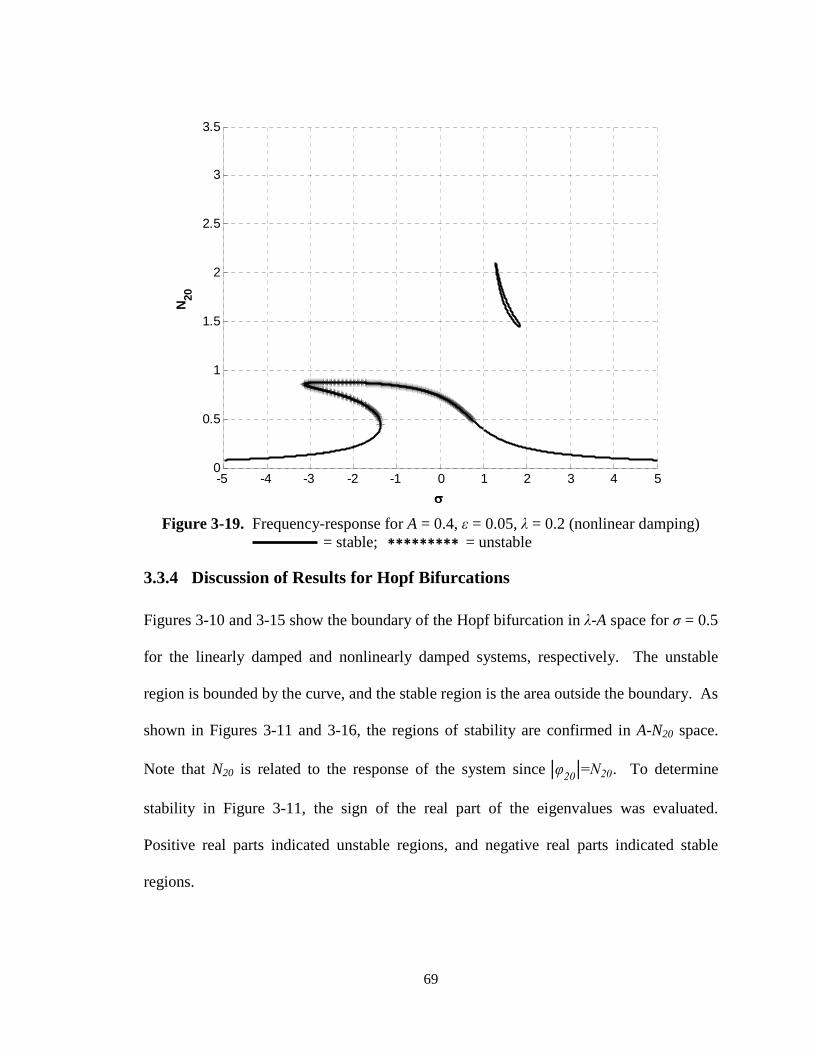
69

Figure 3-19. Frequency-response for A = 0.4, ε = 0.05, λ = 0.2 (nonlinear damping)


3.3.4 Discussion of Results for Hopf Bifurcations

Figures 3-10 and 3-15 show the boundary of the Hopf bifurcation in λ-A space for σ = 0.5

for the linearly damped and nonlinearly damped systems, respectively. The unstable

region is bounded by the curve, and the stable region is the area outside the boundary. As

shown in Figures 3-11 and 3-16, the regions of stability are confirmed in A-N20 space.

Note that N20 is related to the response of the system since ©φ20

©=N20. To determine

stability in Figure 3-11, the sign of the real part of the eigenvalues was evaluated.

Positive real parts indicated unstable regions, and negative real parts indicated stable

regions.

-5 -4 -3 -2 -1 0 1 2 3 4 50

0.5

1

1.5

2

2.5

3

3.5

σσσσ

N20

*********

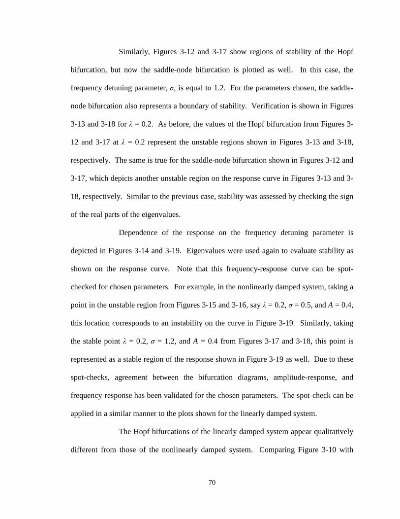
70

Similarly, Figures 3-12 and 3-17 show regions of stability of the Hopf

bifurcation, but now the saddle-node bifurcation is plotted as well. In this case, the

frequency detuning parameter, σ, is equal to 1.2. For the parameters chosen, the saddle-

node bifurcation also represents a boundary of stability. Verification is shown in Figures

3-13 and 3-18 for λ = 0.2. As before, the values of the Hopf bifurcation from Figures 3-

12 and 3-17 at λ = 0.2 represent the unstable regions shown in Figures 3-13 and 3-18,

respectively. The same is true for the saddle-node bifurcation shown in Figures 3-12 and

3-17, which depicts another unstable region on the response curve in Figures 3-13 and 3-

18, respectively. Similar to the previous case, stability was assessed by checking the sign

of the real parts of the eigenvalues.

Dependence of the response on the frequency detuning parameter is

depicted in Figures 3-14 and 3-19. Eigenvalues were used again to evaluate stability as

shown on the response curve. Note that this frequency-response curve can be spot-

checked for chosen parameters. For example, in the nonlinearly damped system, taking a

point in the unstable region from Figures 3-15 and 3-16, say λ = 0.2, σ = 0.5, and A = 0.4,

this location corresponds to an instability on the curve in Figure 3-19. Similarly, taking

the stable point λ = 0.2, σ = 1.2, and A = 0.4 from Figures 3-17 and 3-18, this point is

represented as a stable region of the response shown in Figure 3-19 as well. Due to these

spot-checks, agreement between the bifurcation diagrams, amplitude-response, and

frequency-response has been validated for the chosen parameters. The spot-check can be

applied in a similar manner to the plots shown for the linearly damped system.

The Hopf bifurcations of the linearly damped system appear qualitatively

different from those of the nonlinearly damped system. Comparing Figure 3-10 with

71

Figure 3-15, it is evident that although both plots begin with the same amplitude at λ = 0,

the shapes of the plots are clearly different. The plot given in Figure 3-10 appears

roughly symmetrical about approximately A = 0.65, while the plot for the nonlinearly

damped system given in Figure 3-15 shows a more decreasing trend of the upper branch

and a more leveling trend of the lower branch. In addition, the nonlinearly damped

system bifurcation point occurs at a higher value of λ than that of the linearly damped

system.

Comparing Figure 3-11 with Figure 3-16, there is no apparent change in

the response between the linearly damped and nonlinearly damped systems for the chosen

parameters. However, the boundary of the bifurcations shown in Figures 3-12 and 3-17

are qualitatively different. In the linearly damped system, it can be seen that the

amplitude for the Hopf bifurcation is contained within the amplitude of the saddle-node

bifurcation. However, in the nonlinearly damped system, the amplitude of the Hopf

bifurcation extends past the boundary of the saddle-node bifurcation. This change is

attributed more to a change in the saddle-node bifurcation than the Hopf bifurcation since

in the nonlinearly damped system, the saddle-node bifurcation point occurs at a lower

value of λ than that for the linearly damped system.

The response, N20, shown in Figure 3-13 is qualitatively similar to that

shown in Figure 3-18. For the chosen parameters, the only apparent difference in the

plots is the value of the amplitude, A, at which the upper part of the response changes

direction. In the nonlinearly damped system, this change of direction occurs at a higher

amplitude than that for the linearly damped system.

72

The frequency response plots for both systems (shown in Figures 3-14 and

3-19, respectively) are qualitatively similar as well. The notable changes in the response

characteristics are that for the nonlinearly damped system, the upper part of the lower

response changes direction at a lower value of σ as opposed to the linearly damped

system. Additionally, the upper response of the nonlinearly damped system has a lower

range of response, N20, and σ than that for the linearly damped system.

3.4 Conclusions

As demonstrated in this chapter, the nonlinearly damped system gives qualitatively

different results than the linearly damped system. By simply cubing the velocity

difference in the linearly damped system equations, the system has been modified to

produce clearly different results for chosen parameters. The most notable differences

appear to be the location of the bifurcation points, which set the trend for the plots.

However, the modification of the linear velocity difference to the cubic velocity

difference also changed the appearance of the plots for the saddle-node bifurcations and

chosen parameters for the Hopf bifurcation.

73

3.A Appendix

3.A.1 Saddle-Node Bifurcation Equation Derivations (Linear Damping)

The system is given by

1 ? @ A cos

@ 0.

Let

5 , u .

Making substitutions of the second equation of equations (3.65) into equations (3.64)

gives

u 1 ? @ u A cos

u @ u 0.

From the second equation of equations (3.65) and the second equation of equations

(3.66), the following can be written:

u , u @ u.

Combining equations (3.67), gives

u u @ u.

From the first equation of equations (3.65) and the first equation of equations (3.66), we

can write

5 , A cos u 1 ? @ u.

Combining equations (3.69) results in

5 A cos u 1 ? @ u.

(3.64)

(3.65)

(3.66)

(3.67)

(3.68)

(3.69)

(3.70)

74

In order to eliminate the y1 term from equation (3.70), equations (3.65) can be combined,

resulting in

ª ,

and substitution of equation (3.71) into equation (3.70) leads to

5 A cos u 1 ? ª @ u.

Substituting equations (3.68), (3.71), and (3.72) into equation (3.66) results in

5 1 ? ª A cos

u 1 ? ª 1 u @ 1 u A cos .

Let

o 5 5, o u u.

Rearranging equation (3.74) for φ1 and φ2 gives

5 5 o and u u o, with the complex conjugates

¡ 5 5 o and ¡ u u o. Also, it easily can be verified that

5 5 o, u u o. Expanding the first equation of equations (3.73) and rewriting the cosine term on the

right-hand side of the equation gives

5 5 u o o .

Further manipulation of the right-hand side of the equation gives

5 5 u 1 o o.

(3.71)

(3.72)

(3.73)

(3.74)

(3.75)

(3.76)

(3.77)

(3.78)

(3.79)

75

Multiplying both sides of equation (3.79) by e-it gives

5o 5o uo 1 o .

Equation (3.80) can be rewritten as

5 5 o 1 5o uo 1 o .

Substituting the first equation of equation (3.77) into equation (3.81) and rewriting terms

gives

5o [ uo 1 o ,

which reduces to

5o [ uo 1 o .


5 u o u 5 o 1 o .

Making use of equations (3.75) and (3.76) to eliminate v and w from equation (3.84)

results in

L ¡o ¡oM

21 L ¡o ¡oM

1 o .

Expanding the second equation of equation (3.73) and rewriting the cosine term on the


u 5 u 1 u @ 1 u 1 o o.

(3.80)

(3.81)

(3.85)

(3.83)

(3.84)

(3.82)

(3.86)

76

Using equation (3.77), the second derivative of w can be eliminated as

L o uM 5 u 1 u @ 1 u

1 o o. Multiplying both sides of equation (3.87) by e-it and rewriting gives

uo 5 u o 5 u o 1 u o @ 1 uo 1 o .

Combining terms in equation (3.88) gives

5 u u1 £o 5 u o 1 u o @ 1 uo 1 o .

Equation (3.89) can be reduced to

5 u£o 5 u o 1 u o @ 1 uo 1 o .

Making use of equations (3.75) and (3.76) to eliminate v and w from the second and third

terms in equation (3.90) results in

L ¡o ¡oM

L ¡o ¡oM

1 u o @ 1 uo L1 oM.

But

u o ¡o .

(3.87)

(3.88)

(3.89)

(3.90)

(3.91)

(3.92)

77

Also,

uo ¡o ,

and

LuoM ¡o .

Thus,

LuoM ¡oa 3¡o 3¡o@ .

Noting that

uo LuoMo, we now have

uo o ¡o@ 3¡ 3¡o .

Substituting equations (3.92) and (3.97) into equation (3.91) gives

L ¡o ¡oM

L ¡o ¡oM 1 ¡o @ 1 o ¡o@ 3¡ 3¡o L1 oM.

Omitting the exponential terms from equations (3.85) and (3.98) based on the

justification in Section 3.A.3.1 gives the averaged system

H

1 || .

(3.93)

(3.94)

(3.95)

(3.96)

(3.97)

(3.98)

(3.99)

78

Setting the derivatives of equation (3.99) to zero gives

4 4 4 4

H 4 4 4 4 4

1 |4|4 .

We can rewrite the first equation of equations (3.100) as

4 [ 4 .

Then, after reducing equation (3.101) and rearranging, we have

1 ? 4 1 ? 4 .

Dividing equation (3.102) by (1-σ) gives

4 1 ? 4 . Multiplying both sides of equation (3.103) by 2(1 + ε) / i gives

4 [ .

Substituting Eq. (3.103) into the second equation of equations (3.100) gives

H 4 4 1 ? 4 1 ? 4 [ 4 1 |4|4 .

Multiplying both sides of equation (3.105) by 2 and separating real and imaginary

coefficients of φ20 gives

1 4 [ 1 |4| 4

A

(3.100)

(3.101)

(3.102)

(3.103)

(3.104)

(3.105)

(3.106)

79

Equation (3.106) may be further reduced to

1 4 [ 1 |4| 4,

A ,

then to

1 4 L[M [[ 1 |4| 4,

A , followed by

1 4 [ 1 |4| 4 A . Continuing with the reduction,

1 4 [ 1 |4| 4 A . Dividing by (1 + ε) gives

4 [ [ |4| 4 A . Thus,

4 |4| 4 .

Referring to the derivation in Section 3.A.3.2, we can write

[ [ |4| |4|@ |4|a [ [.


@ 0,

(3.107)

(3.108)

(3.109)

(3.110)

(3.111)

(3.112)

(3.113)

(3.114)

80

where

|4| , [ [

, 1, @ [ [.


3 2 0.

Next, equation (3.116) is solved for Z using the quadratic formula:

[\ ~ [[m\\ .

Substituting this expression for Z into equation (3.114) gives the equation representing

the saddle-node bifurcation boundary:

@ [\ ~ [[m\\ [\ ~ [[m\\

[\ ~ [[m\\ .

3.A.2 Saddle-Node Bifurcation Equation Derivations (Nonlinear Damping)

The nonlinearly damped system is given by

1 ? @ A cos

@ 0.

Let

5 , u .

(3.115)

(3.116)

(3.117)

(3.118)

(3.119)

(3.120)

81

Making substitutions of the second equation of equations (3.120) into equation (3.119)

gives

u 1 ? @ u A cos

u @ u 0.

From the second equation of equations (3.120) and the second equation of equations

(3.121), we can write

u , u @ u.

Combining equations (3.122), we have

u u @ u.

From the first equation of equations (3.120) and the first equation of equations (3.121),

we can write

5 , A cos u 1 ? @ u.

Combining equations (3.124), we have

5 A cos u 1 ? @ u.

In order to eliminate the y1 term from equation (3.125), equations (3.120) can be

combined, resulting in

ª ,

and substitution of equation (3.126) into equation (3.125) leads to

5 A cos u 1 ? ª @ u.

(3.121)

(3.122)

(3.123)

(3.124)

(3.125)

(3.126)

(3.127)

82

Substituting equations (3.123), (3.126), and (3.127) into equations (3.121) results in

5 1 ? ª A cos

u 1 ? ª 1 u @ 1 u A cos .

Let

o 5 5, o u u.

Rearranging equations (3.129) for φ1 and φ2 gives

5 5 o, u u o with the complex conjugates

¡ 5 5 o, ¡ u u o. Also, it easily can be verified that

5 5 o, u u o. Expanding the first equation of equations (3.128) and rewriting the cosine term on the


5 5 u o o .

Further manipulation of the right-hand side of the equation gives

5 5 u 1 o o. Multiplying both sides of equation (3.134) by e-it gives

5o 5o uo 1 o .


5 5 o 1 5o uo 1 o .

(3.128)

(3.129)

(3.130)

(3.131)

(3.132)

(3.133)

(3.134)

(3.135)

(3.136)

83

Substituting the first equation of equations (3.132) into equations (3.136) and rewriting

terms gives

5o [ uo 1 o ,

which reduces to

5o [ uo 1 o .


5 u o u 5 o 1 o .

Making use of equations (3.130) and (3.131) to eliminate v and w from equation (3.139)

results in

L ¡o ¡oM

L ¡o ¡oM 1 o .

Expanding the second equation of equations (3.128) and rewriting the cosine term on the


u 5 u 1 u

@ 1 u 1 o o. Using equation (3.132), the second derivative of w can be eliminated as

L o uM 5 u 1 u @ 1 u

1 o o.

(3.137)

(3.138)

(3.139)

(3.140)

(3.141)

(3.142)

84

Multiplying both sides of equation (3.142) by e-it and rewriting gives

uo 5 u o 5 u o 1 u o @ 1 uo 1 o .

Combining terms in equation (3.143) gives

5 u u1 £o 5 u o 1 u o @ 1 uo 1 o .

Equation (3.144) can be reduced to

5 u£o 5 u o 1 u o @ 1 uo 1 o .

Making use of equations (3.130) and (3.131) to eliminate v and w from the second and

third terms in equation (3.145) results in

L ¡o ¡oM

L ¡o ¡oM

1 u o @ 1 uo L1 oM.

But

u o ¡o ,

and

u o ¡o .

Thus,

u o ¡oa 3¡o 3¡o@ .

(3.143)

(3.144)

(3.145)

(3.146)

(3.147)

(3.148)

(3.149)

85

Noting that

u o Lu oMo, we now have

u o o ¡o@ 3¡ 3¡o .

Also,

uo ¡o ,

and

LuoM ¡o .

Thus,

LuoM ¡oa 3¡o 3¡o@ .

Noting that

uo LuoMo, we now have

uo o ¡o@ 3¡ 3¡o .

Substituting equations (3.151) and (3.156) into equation (3.146) gives

L ¡o ¡oM

L ¡o ¡oM

1 Lo ¡o@ 3¡ 3¡oM @ 1 Lo ¡o@ 3¡ 3¡oM

L1 oM.

(3.150)

(3.151)

(3.152)

(3.153)

(3.154)

(3.155)

(3.156)

(3.157)

86

Omitting the exponential terms from equations (3.140) and (3.157) based on the

justification in Section 3.A.3.1 gives the averaged system

1 ||

1 || .

Setting the derivatives of equations (3.158) to zero gives

4 4 4 4

1 |4|4 4 4 4 4

1 |4|4 .

We can rewrite the first equation of equations (3.159) as

4 [ 4 .

Then, after reducing equation (3.160) and rearranging, we have

1 ? 4 1 ? 4 .

Dividing equation (3.161) by (1-σ) gives

4 1 ? 4 . Multiplying both sides of equation (3.162) by 2(1 + ε) / i gives

4 [ .

Substituting equation (3.162) into the second equation of equations (3.159) gives

1 |4|4 4 1 ? 4 1 ? 4 [ 4 1 |4|4 .

(3.158)

(3.159)

(3.160)

(3.161)

(3.162)

(3.163)

(3.164)

87

Multiplying both sides of equation (3.164) by 2 and separating real and imaginary

coefficients of φ20 gives

@ 1 |4|4

[ 1 |4| 4 A

Equation (3.165) may be further reduced to

@ 1 |4|4 [ 1 |4| 4

A ,

then to

@ 1 |4|4 L[M [[ 1 |4| 4

A , followed by

@ 1 |4|4 [ 1 |4| 4

A . Continuing with the reduction,

@ 1 |4|4 [ 1 |4| 4

A . Dividing by (1 + ε) gives

@ |4|4 [ [ |4| 4 A .

(3.165)

(3.166)

(3.167)

(3.168)

(3.169)

(3.170)

88

Thus,

@ |4|4 |4| 4 .

Referring to the derivation in Section 3.A.3.3, we can write

[ [ |4| |4|@ a 1 |4|a [ [. Referring to equation (3.172), we now have

|4| , [ [ , ,

a 1, @ [ [

Thus, equation (3.172) can be rewritten as

@ 0

The derivative of equation (3.174) with respect to Z is

3 2 0.

Next, equation (3.175) is solved for Z using the quadratic formula:

[\ ~ [[m\\ .

Substituting this expression for Z into equation (3.174) gives the equation representing

the saddle-node bifurcation boundary:

@ [\ ~ [[m\\ [\ ~ [[m\\

[\ ~ [[m\\ .

(3.171)

(3.172)

(3.173)

(3.174)

(3.175)

(3.176)

(3.177)

89

3.A.3 Saddle-Node Bifurcation Analysis Digressions

3.A.3.1 Rationale for Averaged Systems

Equations (3.99) and (3.158) are obtained by taking the average of equations (3.85) and

(3.98) for the linearly damped system and (3.140) and (3.157) for the nonlinearly damped

system. First, understanding the following exponential average should be established.

Over one period, the average value of a function (Stewart, 1999) is given by:

K« ¬ K ¬4 .

If

K o=, then

K« ¬ o=¬4

¬ = To=©4¬

¬= Lo¬= o4M

¬= Lo¬= 1M

But

o¬= cos 2®; ¯w;; sin 2®;

For

|;| 0, 2, 4, 6, …,

we can write

o¬= 1 ¯w;; · 0.

(3.178)

(3.179)

(3.180)

(3.181)

(3.182)

(3.183)

(3.184)

(3.185)

(3.186)

90

Hence

o¬= 1.

Thus,

K« ¬= 1 1 ,

which means

K« 0.

Hence, the averages of e-4it, e-2it, and e2it are all zero.

3.A.3.2 Derivation of Equation (3.113) (Linear Damping)

Beginning with equation (3.112):

4 |4| 4 ,

let

4 P ².

Substituting equation (3.191) into equation (3.190) gives

P ² |4| P ² .

Collecting real and imaginary terms gives

jP |4| ²k j² |4| Pk .

Taking the magnitude of both sides gives

jP |4| ²k j² |4| Pk [ [.

(3.187)

(3.188)

(3.189)

(3.190)

(3.191)

(3.192)

(3.193)

(3.194)

91

Expanding gives

P 2P² |4| |4| ² ²

2P² |4| |4| P [ [. Reducing yields

P ² |4| P ² [ [. But

P ² |4|,

so making this substitution gives

|4| |4| |4| [ [.

Expanding again yields

|4| [ [ |4| |4|@ |4| [ [.

Finally, reducing results in

[ [ |4| |4|@ |4|a [ [.

3.A.3.3 Derivation of Equation (3.172) (Nonlinear Damping)

Beginning with equation (3.171):

@ |4|4 |4| 4 ,

let

4 P ².

Substituting equation (3.202) into equation (3.201) gives

@ |4|P ² |4| P ² .

(3.195)

(3.196)

(3.197)

(3.198)

(3.199)

(3.200)

(3.201)

(3.202)

(3.203)

92

Collecting real and imaginary terms gives

j@ |4|P |4| ²k

j@ |4|² |4| Pk .


j@ |4|P |4| ²k

j@ |4|² |4| Pk [ [.

Expanding gives

a |4|@P |4|P² |4|

|4| ² a |4|@² |4|P² |4| |4| P [ [. Reducing yields

a |4|@P ² |4| P ² [ [. But

P ² |4|,

so making this substitution gives

a |4|a |4| |4| [ [. Expanding again yields

a |4|a [ [ |4| |4|@ |4| [ [.

(3.204)

(3.205)

(3.206)

(3.207)

(3.208)

(3.209)

(3.210)

93

Finally, reducing results in

[ [ |4| |4|@ a 1 |4|a [ [.

3.A.4 Hopf Bifurcation Equation Derivations (Linear Damping)

Let

4 , 4 .

Substituting equation (3.212) into the first equation of equation (3.99) gives

4 4 4

4 4 ,

but the derivative of the fixed point φ10 equals zero. Reducing equation (3.213) further

gives

4 4 4 4 .

Introducing the first equation of equations (3.100) into equation (3.214) and rearranging

gives

. Substituting equation (3.212) into the second equation of equation (3.99) gives

4 H 4 4 4

4 4 1 |4 |4 ,

(3.211)

(3.212)

(3.213)

(3.214)

(3.215)

(3.216)

94

but the derivative of the fixed point φ20 equals zero, and by the derivation in Section

3.A.6.1,

|4 |4 > |4|4 2|4| ¡4.

Thus, equation (3.216) can be reduced to

H

1 |4|4 2|4| ¡4£ H 4

4 4 4 4 .

Equation (3.218) can be further reduced to

H

1 |4| 1 ¡4 H 4

4 4 4 4 1 |4|4 .

Introducing the second equation of equations (3.100) into equation (3.219) and

rearranging gives

H

1 |4| 4¡. From equations (3.215) and (3.220), we can write

¡ ¡ ¡ ¡ ¡

and

¡ H ¡ ¡ ¡ ¡ ¡

1 |4|¡ 4¡ .

(3.217)

(3.218)

(3.219)

(3.220)

(3.221)

(3.222)

95

Now we can construct the matrix F = [ δ1; δ1*; δ2; δ2

*] . Using MATLAB, the Jacobian

matrix was computed. From the MATLAB output and substituting in

|4| q4, q4@ 44¡ ,

we develop the relations

¢ 1 ,

¢ ³ @ @ ´ q4@ ? 1 q4 @ 1 @ ? 1 , ¢ @ ? 1 ,

¢@ a 1 ? q4@ @ ?1 ? q4 a 1 ? ?£, in which the characteristic polynomial is given by

@ ¢ ¢ ¢ ¢@ 0.

For the Hopf bifurcation to occur, we must have

~Ω,



Ω@ ¢Ω ¢@ 0, Ω¢Ω ¢ 0 ¥ Ω ¦\¦m.

Substituting the relation for Ω2 into the first equation of equations (3.227) and reducing

gives

¢ ¢¢¢ ¢@¢ 0.


5§ 5§ 5 0,


§, [¨[[@\mm ,

(3.223)

(3.224)

(3.225)

(3.226)

(3.227)

(3.228)

(3.229)

(3.230)

96

and from equation (3.114), we have the boundaries of stability, given by

§ § § @ 0; § ; 1,2.

The remainder of this analysis is carried out using MATLAB.

3.A.5 Hopf Bifurcation Equation Derivations (Nonlinear Damping)

Let

4 , 4 .

Substituting equation (3.231) into the first equation of equations (3.158) gives

4 4 4

4 4 ,

but the derivative of the fixed point φ10 equals zero. Reducing equation (3.232) further

gives

4 4 4 4 .

Introducing the first equation of equations (3.159) into equation (3.233) and rearranging

gives

. Substituting equations (3.231) into the second equation of equations (3.158) gives

4 H ^ |4 |4 4 4

4 4 1 |4 |4 ,

(3.231)

(3.232)

(3.233)

(3.234)

(3.235)

97

but the derivative of the fixed point φ20 equals zero, and by the derivation in Section

3.A.6.1,

|4 |4 > |4|4 2|4| ¡4.

Thus, equation (3.235) can be reduced to

H ^ |4|4 2|4| ¡4£ 4 4 4 4 .

Equation (3.237) can be further reduced to

H @ 1 |4| H ^ ¡4

4 4 4 4 H ^ |4|4 .

Introducing the second equation of equations (3.159) into equation (3.238) and

rearranging gives

H @ |4| 1 |4| H ^ 4¡ 4¡. From equations (3.234) and (3.239), we can write

¡ ¡ ¡ ¡ ¡

and

¡ ¡ ¡ ¡ ¡

H @ |4|¡ 1 |4|¡ H ^ 4¡ 4¡ .

(3.236)

(3.237)

(3.238)

(3.239)

(3.240)

(3.241)

98

Now we can construct the matrix F = [ δ1; δ1*; δ2; δ2

*] . Using MATLAB, the Jacobian

matrix was computed. From the MATLAB output and substituting in

|4| q4, q4@ 44¡ ,

we develop the relations

¢ H 1 q4,

¢ ³µ[H[a@ µH[ µH[a@ [@ @´ q4@

? 1 q4 14 ? 1 , ¢ H^ 1 ? q4,

¢@ ³µ[H[[ca µ[H[^ µ[H[ca [[a [^ [a ´ q4@

@ ?1 ? q4 [[a ,

in which the characteristic polynomial is given by

@ ¢ ¢ ¢ ¢@ 0.

For the Hopf bifurcation to occur, we must have

~Ω,



Ω@ ¢Ω ¢@ 0, Ω¢Ω ¢ 0 ¥ Ω ¦\¦m.

Substituting the relation for Ω2 into the first equation of equations (3.246) and reducing

gives

¢ ¢¢¢ ¢@¢ 0.

(3.242)

(3.243)

(3.244)

(3.245)

(3.246)

(3.247)

99

Letting z = N202, equations (3.243) can be rewritten as

¢ H 1 §,

¢ ³µ[H[a@ µH[ µH[a@ [@ @´ §

? 1 § 14 ? 1 , ¢ H^ 1 ? §,

¢@ ³µ[H[[ca µ[H[^ µ[H[ca [[a [^ [a ´ §

@ ?1 ? § [[a .

MATLAB was used to determine the coefficients

5 µ4@ 9 16 ? 1 1 ,

5 a ? 1 ? 1 1 ,

5 a@ ? 1 ,

for

5§ 5§ 5 0,


§, [¨[[@\mm ,

and from equation (3.174), we have the boundaries of stability, given by

§ § § @ 0; § ; 1,2.

The remainder of this analysis is carried out using MATLAB.

(3.248)

(3.249)

(3.250)

(3.251)

(3.252)

100

3.A.6 Hopf Bifurcation Analysis Digressions

3.A.6.1 Derivation of Equations (3.217) and (3.236)

Let

4 P ², e Then,

4¡ P ². 44¡ P ² P ²

P ² |4|

Thus,

44¡ |4|,

and by similarity,

¡ ||.

Additionally,

|4 | |P ² e |

|P e ² |

P e ² ,

and

4 4¡ ¡ P ² e P ² e

P e ² £P e ² £ P e ²

|P e ² |.

(3.253)

(3.254)

(3.255)

(3.256)

(3.257)

(3.258)

(3.259)

(3.260)

101

Thus,

|4 | 4 4¡ ¡ .

Continuing with the derivation,

|4 |4 4 4¡ ¡ 4

44¡ ¡4 4¡ ¡ 4

|4| ¡4 4¡ || 4

|4|4 |4| ¡4 ¡4

44¡ 4¡ ||4

|4|4 |4| ¡4 ||4

|4| 4¡ ||4

|4|4 2|4| ¡4

||4 4¡ ||4

Omitting nonlinear terms (specifically, terms containing |δ2|2 and δ2

2), the equation is

reduced to

|4 |4 |4|4 2|4| ¡4.

(3.261)

(3.262)

(3.263)

(3.264)

(3.265)

(3.266)

(3.267)

(3.268)

102

3.A.6.2 Derivation of Equivalent Expression for N204

Let

4 P ², 4¡ P ². Then,

44¡ P ² P ²

P@ 2P² ²@

P ²

|4|@.

Since |φ20| = N20, then |φ20|4 = N20

4. Thus,

44¡ q4@.

(3.269)

(3.270)

(3.271)

(3.272)

(3.273)

(3.274)

103

3.A.7 MATLAB Code

3.A.7.1 Saddle-Node Example close all clear all mu = [0:0.01:5]; xp = sqrt(mu); xn = -sqrt(mu); figure plot(mu,xp, '-k' ,mu,xn, '--k' , 'LineWidth' ,2) xlim([-2 2]); ylim([-2 2]); xlabel( '\fontsize12\bf\mu' ); ylabel( '\bfx' ); grid on; legend( '\bfstable' , '\bfunstable' , 'Location' , 'NorthWest' )

3.A.7.2 Solving for Z for Saddle-Node Plots

close all clear all syms a1 a2 a3 a4 Z z = solve( 'a1*Z + a2*Z^2 + a3*Z^3 + a4 = 0' , Z); z1 = simple(z(1)) z2 = simple(z(2)) z3 = simple(z(3))

3.A.7.3 Saddle-Node Plots (Linear Damping) %Saddle-Node Bifurcation - Linear Damping %(boundaries of number of real periodic solutions) close all clear all n_sigma = 0; k2 = 0; for sigma = [1.2 2 5 7 -0.5 -2 -5 -7 3]; k2 = k2+1; sigma_vec(k2) = sigma; k = 0; n_sigm a = n_sigma + 1; for lambda = 0:.001:4 k = k+1; a1 = lambda^2 + sigma^2/(1 - sigma)^2; a2 = 2*sigma/(1 - sigma); a3 = 1;

104

%Solving for a4: a4_p = -a1*(-a2/(3*a3) + sqrt(a2^2 - 3*a1*a 3)/(3*a3)) - ... a2*(-a2/(3*a3) + sqrt(a2^2 - 3*a1*a3)/( 3*a3))^2 - ... a3*(-a2/(3*a3) + sqrt(a2^2 - 3*a1*a3)/( 3*a3))^3; a4_m = -a1*(-a2/(3*a3) - sqrt(a2^2 - 3*a1*a 3)/(3*a3)) - ... a2*(-a2/(3*a3) - sqrt(a2^2 - 3*a1*a3)/( 3*a3))^2 - ... a3*(-a2/(3*a3) - sqrt(a2^2 - 3*a1*a3)/( 3*a3))^3; %Solving for A from a4: A_p = sqrt(-a4_p*(1-sigma)^2); A_m = sqrt(- a4_m*(1-sigma)^2); lambda_vec(k) = lambda; A_p_vec(k) = A_p; A _m_vec(k) = A_m; end m = k; g = ones(1,k); h = ones(1,k); for n = 1:k if abs(A_p_vec(n)- A_m_vec(n)) < .0001 g(n) = 0; h(n) = 0; elseif n > 1 && g(n-1) == 0 && h(n-1) == 0 m = m-1; g(n) = 0; h(n) = 0; else end end lambda_vec_2 = zeros(1,m); A_p_vec_2 = zeros(1,m); A_m_vec_2 = zeros(1,m); for q = 1:m lambda_vec_2(q) = lambda_vec(q); A_p_vec_2(q) = A_p_vec(q); A_m_vec_2(q) = A_m_vec(q); end if n_sigma == 1 %sigma = 1.2 figure xlabel( '\fontsize12\bf\lambda' ); ylabel( '\bfA' ); hold on; axis([0 3.5 0 4.5]) plot(lambda_vec_2, A_p_vec_2, ':k' , 'LineWidth' ,2) plot(lambda_vec_2, A_m_vec_2, ':k' , 'LineWidth' ,2) text(3, 1.2, [ '\fontsize14\bf\sigma\fontsize12 = ' , ... num2str(sigma_vec(n_sigma))]) elseif n_sigma == 2 %sigma = 2 plot(lambda_vec_2, A_p_vec_2, '-k' , 'LineWidth' ,2) plot(lambda_vec_2, A_m_vec_2, '-k' , 'LineWidth' ,2) text(1.2, 1.5, [ '\fontsize14\bf\sigma\fontsize12 = ' , ... num2str(sigma_vec(n_sigma))]) elseif n_sigma == 3 %sigma = 5 plot(lambda_vec_2, A_p_vec_2, '--k' , 'LineWidth' ,2) plot(lambda_vec_2, A_m_vec_2, '--k' , 'LineWidth' ,2)

105

text(0.7, 2.5, [ '\fontsize14\bf\sigma\fontsize12 = ' , ... num2str(sigma_vec(n_sigma))]) elseif n_sigma == 4 %sigma = 7 plot(lambda_vec_2, A_p_vec_2, '-.k' , 'LineWidth' ,2) plot(lambda_vec_2, A_m_vec_2, '-.k' , 'LineWidth' ,2) text(.7, 3.7, [ '\fontsize14\bf\sigma\fontsize12 = ' , ... num2str(sigma_vec(n_sigma))]) elseif n_sigma == 5 %sigma = -0.5 figure xlabel( '\fontsize12\bf\lambda' ); ylabel( '\bfA' ); hold on; axis([0 0.8 0 4]) plot(lambda_vec_2, A_p_vec_2, ':k' , 'LineWidth' ,2) plot(lambda_vec_2, A_m_vec_2, ':k' , 'LineWidth' ,2) text(0.21, 0.18, [ '\fontsize14\bf\sigma\fontsize12 = ' , ... num2str(sigma_vec(n_sigma))]) elseif n_sigma == 6 %sigma = -2 plot(lambda_vec_2, A_p_vec_2, '-k' , 'LineWidth' ,2) plot(lambda_vec_2, A_m_vec_2, '-k' , 'LineWidth' ,2) text(0.4, 0.8, [ '\fontsize14\bf\sigma\fontsize12 = ' , ... num2str(sigma_vec(n_sigma))]) elseif n_sigma == 7 %sigma = -5 plot(lambda_vec_2, A_p_vec_2, '--k' , 'LineWidth' ,2) plot(lambda_vec_2, A_m_vec_2, '--k' , 'LineWidth' ,2) text(0.48, 2.2, [ '\fontsize14\bf\sigma\fontsize12 = ' , ... num2str(sigma_vec(n_sigma))]) elseif n_sigma == 8 %sigma = -7 plot(lambda_vec_2, A_p_vec_2, '-.k' , 'LineWidth' ,2) plot(lambda_vec_2, A_m_vec_2, '-.k' , 'LineWidth' ,2) text(0.5, 3.25, [ '\fontsize14\bf\sigma\fontsize12 = ' , ... num2str(sigma_vec(n_sigma))]) else end if n_sigma == 9 %sigma = 3 figure axis([0 1 0 2.5]) xlabel( '\fontsize12\bf\lambda' ); ylabel( '\bfA' ); hold on; plot(lambda_vec_2, A_p_vec_2, '-k' , 'LineWidth' ,2) plot(lambda_vec_2, A_m_vec_2, '-k' , 'LineWidth' ,2) else end end %************************************************** *********************** %************************************************** ***********************

106

%************************************************** *********************** %Check number of solutions within boundaries by sub stitution: clear all n = 0; for sigma = [3 1.2 2 5 7 -0.5 -2 -5 -7]; if sigma == 3; lambda = 0.3; for A = [0.2, 1, 1.7]; n = n + 1; a1v(n) = lambda^2 + sigma^2/(1 - sigma) ^2; a2v(n) = 2*sigma/(1 - sigma); a3v(n) = 1; a4v(n) = -A^2/(1-sigma)^2; sigma_vec(n) = sigma; A_vec(n) = A; lam _vec(n) = lambda; end elseif sigma == 1.2 lambda = 0.3; for A = [0.2, 0.75, 1.6]; n = n + 1; a1v(n) = lambda^2 + sigma^2/(1 - sigma) ^2; a2v(n) = 2*sigma/(1 - sigma); a3v(n) = 1; a4v(n) = -A^2/(1-sigma)^2; sigma_vec(n) = sigma; A_vec(n) = A; lam _vec(n) = lambda; end elseif sigma == 2 lambda = 0.3; for A = [0.2, 0.75, 1.6]; n = n + 1; a1v(n) = lambda^2 + sigma^2/(1 - sigma) ^2; a2v(n) = 2*sigma/(1 - sigma); a3v(n) = 1; a4v(n) = -A^2/(1-sigma)^2; sigma_vec(n) = sigma; A_vec(n) = A; lam _vec(n) = lambda; end elseif sigma == 5 lambda = 0.3; for A = [0.2, 1.6, 2.5]; n = n + 1; a1v(n) = lambda^2 + sigma^2/(1 - sigma) ^2; a2v(n) = 2*sigma/(1 - sigma); a3v(n) = 1; a4v(n) = -A^2/(1-sigma)^2; sigma_vec(n) = sigma; A_vec(n) = A; lam _vec(n) = lambda; end elseif sigma == 7 lambda = 0.3; for A = [0.5, 2.5, 3.5]; n = n + 1; a1v(n) = lambda^2 + sigma^2/(1 - sigma) ^2;

107

a2v(n) = 2*sigma/(1 - sigma); a3v(n) = 1; a4v(n) = -A^2/(1-sigma)^2; sigma_vec(n) = sigma; A_vec(n) = A; lam _vec(n) = lambda; end elseif sigma == -0.5 lambda = 0.3; for A = [0.01, 0.1, 0.5]; n = n + 1; a1v(n) = lambda^2 + sigma^2/(1 - sigma) ^2; a2v(n) = 2*sigma/(1 - sigma); a3v(n) = 1; a4v(n) = -A^2/(1-sigma)^2; sigma_vec(n) = sigma; A_vec(n) = A; lam _vec(n) = lambda; end elseif sigma == -2 lambda = 0.3; for A = [0.1, 0.5, 1]; n = n + 1; a1v(n) = lambda^2 + sigma^2/(1 - sigma) ^2; a2v(n) = 2*sigma/(1 - sigma); a3v(n) = 1; a4v(n) = -A^2/(1-sigma)^2; sigma_vec(n) = sigma; A_vec(n) = A; lam _vec(n) = lambda; end elseif sigma == -5 lambda = 0.3; for A = [0.5, 1.5, 2]; n = n + 1; a1v(n) = lambda^2 + sigma^2/(1 - sigma) ^2; a2v(n) = 2*sigma/(1 - sigma); a3v(n) = 1; a4v(n) = -A^2/(1-sigma)^2; sigma_vec(n) = sigma; A_vec(n) = A; lam _vec(n) = lambda; end elseif sigma == -7 lambda = 0.3; for A = [0.5, 2, 3]; n = n + 1; a1v(n) = lambda^2 + sigma^2/(1 - sigma) ^2; a2v(n) = 2*sigma/(1 - sigma); a3v(n) = 1; a4v(n) = -A^2/(1-sigma)^2; sigma_vec(n) = sigma; A_vec(n) = A; lam _vec(n) = lambda; end else end end for k = 1:n %Values for Z1, Z2, and Z3 were obtained by solving equation (3.15): a1 = a1v(k); a2 = a2v(k); a3 = a3v(k); a4 = a4v (k);

108

Z1 = ((a1^3/(27*a3^3) + a4^2/(4*a3^2) + (a2^3*a 4)/(27*a3^4) - ... (a1^2*a2^2)/(108*a3^4) - (a1*a2*a4)/(6*a3^3 ))^(1/2) - ... a4/(2*a3) - a2^3/(27*a3^3) + (a1*a2)/(6*a3^ 2))^(1/3) - ... a2/(3*a3) - (a1/(3*a3) - a2^2/(9*a3^2))/((a 1^3/(27*a3^3) + ... a4^2/(4*a3^2) + (a2^3*a4)/(27*a3^4) - (a1^2 *a2^2)/(108*a3^4) - ... (a1*a2*a4)/(6*a3^3))^(1/2) - a4/(2*a3) - a2 ^3/(27*a3^3) + ... (a1*a2)/(6*a3^2))^(1/3); Z2 = -(a3^2*(3*3^(1/2)*1i + 3)*(-(27*a3^2*a4 - 54*a3^3*((4*a1^3*a3 - ... a1^2*a2^2 - 18*a1*a2*a3*a4 + 4*a2^3*a4 + ... 27*a3^2*a4^2)/(108*a3^4))^(1/2) + 2*a2^3 - ... 9*a1*a2*a3)/(54*a3^3))^(2/3) - a2^2*((3^(1/ 2)*1i)/3 - 1/3) + ... a1*a3*(3^(1/2)*1i - 1) + 2*a2*a3*(-(27*a3^2 *a4 - ... 54*a3^3*((4*a1^3*a3 - a1^2*a2^2 - 18*a1*a2* a3*a4 + 4*a2^3*a4 + ... 27*a3^2*a4^2)/(108*a3^4))^(1/2) + 2*a2^3 - ... 9*a1*a2*a3)/(54*a3^3))^(1/3))/(6*a3^2*(-(27 *a3^2*a4 - ... 54*a3^3*((4*a1^3*a3 - a1^2*a2^2 - 18*a1*a2* a3*a4 + 4*a2^3*a4 + ... 27*a3^2*a4^2)/(108*a3^4))^(1/2) + 2*a2^3 - ... 9*a1*a2*a3)/(54*a3^3))^(1/3)); Z3 = -(a2^2*((3^(1/2)*1i)/3 + 1/3) - a3^2*(3*3^ (1/2)*1i - ... 3)*(-(27*a3^2*a4 - 54*a3^3*((4*a1^3*a3 - a1 ^2*a2^2 - ... 18*a1*a2*a3*a4 + 4*a2^3*a4 + 27*a3^2*a4^2)/ (108*a3^4))^(1/2) + ... 2*a2^3 - 9*a1*a2*a3)/(54*a3^3))^(2/3) - a1* a3*(3^(1/2)*1i + ... 1) + 2*a2*a3*(-(27*a3^2*a4 - 54*a3^3*((4*a1 ^3*a3 - a1^2*a2^2 - ... 18*a1*a2*a3*a4 + 4*a2^3*a4 + 27*a3^2*a4^2)/ (108*a3^4))^(1/2) + ... 2*a2^3 - 9*a1*a2*a3)/(54*a3^3))^(1/3))/(6*a 3^2*(-(27*a3^2*a4 - ... 54*a3^3*((4*a1^3*a3 - a1^2*a2^2 - 18*a1*a2* a3*a4 + 4*a2^3*a4 + ... 27*a3^2*a4^2)/(108*a3^4))^(1/2) + 2*a2^3 - ... 9*a1*a2*a3)/(54*a3^3))^(1/3)); %Eliminate approximation errors: if abs(imag(Z1)) < 0.00001 Z1 = real(Z1); else end if abs(imag(Z2)) < 0.00001 Z2 = real(Z2); else end if abs(imag(Z3)) < 0.00001 Z3 = real(Z3); else

109

end if k == 1 plot(lam_vec(k), A_vec(k), '*k' ) text(lam_vec(k) + 0.03,A_vec(k)+0.24,[ '\fontsize12\bf\lambda' ... '\fontsize10 = ' , num2str(lam_vec(k)), ', A = ' , ... num2str(A_vec(k))], 'FontSize' ,10) text(lam_vec(k) + 0.03, A_vec(k)+0.12, [ '\bfZ_1 = ' , num2str(Z1)]) text(lam_vec(k) + 0.03, A_vec(k), [ '\bfZ_2 = ' , num2str(Z2)]) text(lam_vec(k) + 0.03, A_vec(k)-0.12, [ '\bfZ_3 = ' , num2str(Z3)]) elseif k == 2 plot(lam_vec(k), A_vec(k), '*k' ) text(lam_vec(k) - 0.21,A_vec(k)+0.24,[ '\fontsize12\bf\lambda' ... '\fontsize10 = ' , num2str(lam_vec(k)), ', A = ' , ... num2str(A_vec(k))], 'FontSize' ,10) text(lam_vec(k) - 0.21, A_vec(k)+0.12, [ '\bfZ_1 = ' , num2str(Z1)]) text(lam_vec(k) - 0.21, A_vec(k), [ '\bfZ_2 = ' , num2str(Z2)]) text(lam_vec(k) - 0.21, A_vec(k)-0.12, [ '\bfZ_3 = ' , num2str(Z3)]) elseif k == 3 plot(lam_vec(k), A_vec(k), '*k' ) text(lam_vec(k) + 0.03,A_vec(k)+0.48,[ '\fontsize12\bf\lambda' ... '\fontsize10 = ' , num2str(lam_vec(k)), ', A = ' , ... num2str(A_vec(k))], 'FontSize' ,10) text(lam_vec(k) + 0.03, A_vec(k)+0.36, [ '\bfZ_1 = ' , num2str(Z1)]) text(lam_vec(k) + 0.03, A_vec(k)+.24, [ '\bfZ_2 = ' , num2str(Z2)]) text(lam_vec(k) + 0.03, A_vec(k)+.12, [ '\bfZ_3 = ' , num2str(Z3)]) else end %Check number of real periodic solutions: if abs(imag(Z1)) > 0 && abs(imag(Z2)) > 0 && abs(imag (Z3)) > 0 num_sol(k) = 0; sigma_out(k) = sigma_vec(k) ; lambda_out(k) = lam_vec(k); A_out(k) = A_ve c(k); elseif abs(imag(Z1)) == 0 && abs(imag(Z2)) > 0 && abs(ima g(Z3)) > 0 num_sol(k) = 1; sigma_out(k) = sigma_vec(k) ; lambda_out(k) = lam_vec(k); A_out(k) = A_ve c(k); elseif abs(imag(Z1)) > 0 && abs(imag(Z2)) == 0 && abs(ima g(Z3)) > 0 num_sol(k) = 1; sigma_out(k) = sigma_vec(k) ; lambda_out(k) = lam_vec(k); A_out(k) = A_ve c(k); elseif abs(imag(Z1)) > 0 && abs(imag(Z2)) > 0 && abs(imag (Z3)) == 0 num_sol(k) = 1; sigma_out(k) = sigma_vec(k) ; lambda_out(k) = lam_vec(k); A_out(k) = A_ve c(k); elseif abs(imag(Z1)) == 0 && abs(imag(Z2)) == 0 && abs(im ag(Z3)) == 0 num_sol(k) = 3; sigma_out(k) = sigma_vec(k) ;

110

lambda_out(k) = lam_vec(k); A_out(k) = A_ve c(k); else num_sol(k) = 2; sigma_out(k) = sigma_vec(k) ; lambda_out(k) = lam_vec(k); A_out(k) = A_ve c(k); end end

3.A.7.4 Saddle-Node Plots (Nonlinear Damping) %Saddle-Node Bifurcation - Nonlinear Damping %(boundaries of number of real periodic solutions) close all clear all n_sigma = 0; k2 = 0; for sigma = [1.2 2 5 7 -0.5 -2 -5 -7 3]; k2 = k2+1; sigma_vec(k2) = sigma; k = 0; n_sigm a = n_sigma + 1; for lambda = 0:.001:4 k = k+1; a1 = sigma^2/(1 - sigma)^2; a2 = 2*sigma/(1 - sigma); a3 = (9/16)*lambda^2 + 1; %Solving for a4: a4_p = -a1*(-a2/(3*a3) + sqrt(a2^2 - 3*a1*a 3)/(3*a3)) - ... a2*(-a2/(3*a3) + sqrt(a2^2 - 3*a1*a3)/( 3*a3))^2 - ... a3*(-a2/(3*a3) + sqrt(a2^2 - 3*a1*a3)/( 3*a3))^3; a4_m = -a1*(-a2/(3*a3) - sqrt(a2^2 - 3*a1*a 3)/(3*a3)) - ... a2*(-a2/(3*a3) - sqrt(a2^2 - 3*a1*a3)/( 3*a3))^2 - ... a3*(-a2/(3*a3) - sqrt(a2^2 - 3*a1*a3)/( 3*a3))^3; %Solving for A from a4: A_p = sqrt(-a4_p*(1-sigma)^2); A_m = sqrt(- a4_m*(1-sigma)^2); lambda_vec(k) = lambda; A_p_vec(k) = A_p; A _m_vec(k) = A_m; end m = k; g = ones(1,k); h = ones(1,k); for n = 1:k if abs(A_p_vec(n)- A_m_vec(n)) < .0001 g(n) = 0; h(n) = 0; elseif n > 1 && g(n-1) == 0 && h(n-1) == 0 m = m-1; g(n) = 0; h(n) = 0; else end end

111

lambda_vec_2 = zeros(1,m); A_p_vec_2 = zeros(1,m); A_m_vec_2 = zeros(1,m); for q = 1:m lambda_vec_2(q) = lambda_vec(q); A_p_vec_2(q) = A_p_vec(q); A_m_vec_2(q) = A_m_vec(q); end if n_sigma == 1 %sigma = 1.2 figure xlabel( '\fontsize12\bf\lambda' ); ylabel( '\bfA' ); hold on; axis([0 3.5 0 4.5]) plot(lambda_vec_2, A_p_vec_2, ':k' , 'LineWidth' ,2) plot(lambda_vec_2, A_m_vec_2, ':k' , 'LineWidth' ,2) text(0.7, 1.4, [ '\fontsize14\bf\sigma\fontsize12 = ' , ... num2str(sigma_vec(n_sigma))]) elseif n_sigma == 2 %sigma = 2 plot(lambda_vec_2, A_p_vec_2, '-k' , 'LineWidth' ,2) plot(lambda_vec_2, A_m_vec_2, '-k' , 'LineWidth' ,2) text(0.7, 0.9, [ '\fontsize14\bf\sigma\fontsize12 = ' , ... num2str(sigma_vec(n_sigma))]) elseif n_sigma == 3 %sigma = 5 plot(lambda_vec_2, A_p_vec_2, '--k' , 'LineWidth' ,2) plot(lambda_vec_2, A_m_vec_2, '--k' , 'LineWidth' ,2) text(0.7, 2.5, [ '\fontsize14\bf\sigma\fontsize12 = ' , ... num2str(sigma_vec(n_sigma))]) elseif n_sigma == 4 %sigma = 7 plot(lambda_vec_2, A_p_vec_2, '-.k' , 'LineWidth' ,2) plot(lambda_vec_2, A_m_vec_2, '-.k' , 'LineWidth' ,2) text(0.7, 3.3, [ '\fontsize14\bf\sigma\fontsize12 = ' , ... num2str(sigma_vec(n_sigma))]) elseif n_sigma == 5 %sigma = -0.5 figure xlabel( '\fontsize12\bf\lambda' ); ylabel( '\bfA' ); hold on; axis([0 0.8 0 4]) plot(lambda_vec_2, A_p_vec_2, ':k' , 'LineWidth' ,2) plot(lambda_vec_2, A_m_vec_2, ':k' , 'LineWidth' ,2) text(0.7, 0.25, [ '\fontsize14\bf\sigma\fontsize12 = ' , ... num2str(sigma_vec(n_sigma))]) elseif n_sigma == 6 %sigma = -2 plot(lambda_vec_2, A_p_vec_2, '-k' , 'LineWidth' ,2) plot(lambda_vec_2, A_m_vec_2, '-k' , 'LineWidth' ,2) text(0.7, 0.8, [ '\fontsize14\bf\sigma\fontsize12 = ' , ... num2str(sigma_vec(n_sigma))]) elseif n_sigma == 7 %sigma = -5

112

plot(lambda_vec_2, A_p_vec_2, '--k' , 'LineWidth' ,2) plot(lambda_vec_2, A_m_vec_2, '--k' , 'LineWidth' ,2) text(0.7, 2, [ '\fontsize14\bf\sigma\fontsize12 = ' , ... num2str(sigma_vec(n_sigma))]) elseif n_sigma == 8 %sigma = -7 plot(lambda_vec_2, A_p_vec_2, '-.k' , 'LineWidth' ,2) plot(lambda_vec_2, A_m_vec_2, '-.k' , 'LineWidth' ,2) text(0.7, 2.8, [ '\fontsize14\bf\sigma\fontsize12 = ' , ... num2str(sigma_vec(n_sigma))]) else end if n_sigma == 9 %sigma = 3 figure axis([0 1 0 2.5]) xlabel( '\fontsize12\bf\lambda' ); ylabel( '\bfA' ); hold on; plot(lambda_vec_2, A_p_vec_2, '-k' , 'LineWidth' ,2) plot(lambda_vec_2, A_m_vec_2, '-k' , 'LineWidth' ,2) else end end %************************************************** *********************** %************************************************** *********************** %************************************************** *********************** %Check number of solutions within boundaries by sub stitution: clear all n = 0; for sigma = [3 1.2 2 5 7 -0.5 -2 -5 -7]; if sigma == 3; lambda = 0.3; for A = [0.2, 1, 1.7]; n = n + 1; a1v(n) = sigma^2/(1 - sigma)^2; a2v(n) = 2*sigma/(1 - sigma); a3v(n) = (9/16)*lambda^2 + 1; a4v(n) = -A^2/(1-sigma)^2; sigma_vec(n) = sigma; A_vec(n) = A; lam _vec(n) = lambda; end elseif sigma == 1.2 lambda = 0.3; for A = [0.2, 0.75, 1.6]; n = n + 1; a1v(n) = sigma^2/(1 - sigma)^2; a2v(n) = 2*sigma/(1 - sigma);

113

a3v(n) = (9/16)*lambda^2 + 1; a4v(n) = -A^2/(1-sigma)^2; sigma_vec(n) = sigma; A_vec(n) = A; lam _vec(n) = lambda; end elseif sigma == 2 lambda = 0.3; for A = [0.2, 0.75, 1.6]; n = n + 1; a1v(n) = sigma^2/(1 - sigma)^2; a2v(n) = 2*sigma/(1 - sigma); a3v(n) = (9/16)*lambda^2 + 1; a4v(n) = -A^2/(1-sigma)^2; sigma_vec(n) = sigma; A_vec(n) = A; lam _vec(n) = lambda; end elseif sigma == 5 lambda = 0.3; for A = [0.2, 1.6, 2.5]; n = n + 1; a1v(n) = sigma^2/(1 - sigma)^2; a2v(n) = 2*sigma/(1 - sigma); a3v(n) = (9/16)*lambda^2 + 1; a4v(n) = -A^2/(1-sigma)^2; sigma_vec(n) = sigma; A_vec(n) = A; lam _vec(n) = lambda; end elseif sigma == 7 lambda = 0.3; for A = [0.5, 2.5, 3.5]; n = n + 1; a1v(n) = sigma^2/(1 - sigma)^2; a2v(n) = 2*sigma/(1 - sigma); a3v(n) = (9/16)*lambda^2 + 1; a4v(n) = -A^2/(1-sigma)^2; sigma_vec(n) = sigma; A_vec(n) = A; lam _vec(n) = lambda; end elseif sigma == -0.5 lambda = 0.3; for A = [0.01, 0.1, 0.5]; n = n + 1; a1v(n) = sigma^2/(1 - sigma)^2; a2v(n) = 2*sigma/(1 - sigma); a3v(n) = (9/16)*lambda^2 + 1; a4v(n) = -A^2/(1-sigma)^2; sigma_vec(n) = sigma; A_vec(n) = A; lam _vec(n) = lambda; end elseif sigma == -2 lambda = 0.3; for A = [0.1, 0.5, 1]; n = n + 1; a1v(n) = sigma^2/(1 - sigma)^2; a2v(n) = 2*sigma/(1 - sigma); a3v(n) = (9/16)*lambda^2 + 1; a4v(n) = -A^2/(1-sigma)^2; sigma_vec(n) = sigma; A_vec(n) = A; lam _vec(n) = lambda; end elseif sigma == -5 lambda = 0.3; for A = [0.5, 1.5, 2];

114

n = n + 1; a1v(n) = sigma^2/(1 - sigma)^2; a2v(n) = 2*sigma/(1 - sigma); a3v(n) = (9/16)*lambda^2 + 1; a4v(n) = -A^2/(1-sigma)^2; sigma_vec(n) = sigma; A_vec(n) = A; lam _vec(n) = lambda; end elseif sigma == -7 lambda = 0.3; for A = [0.5, 2, 3]; n = n + 1; a1v(n) = sigma^2/(1 - sigma)^2; a2v(n) = 2*sigma/(1 - sigma); a3v(n) = (9/16)*lambda^2 + 1; a4v(n) = -A^2/(1-sigma)^2; sigma_vec(n) = sigma; A_vec(n) = A; lam _vec(n) = lambda; end else end end for k = 1:n %Values for Z1, Z2, and Z3 were obtained by solving equation (3.24). a1 = a1v(k); a2 = a2v(k); a3 = a3v(k); a4 = a4v (k); Z1 = ((a1^3/(27*a3^3) + a4^2/(4*a3^2) + (a2^3*a 4)/(27*a3^4) - ... (a1^2*a2^2)/(108*a3^4) - (a1*a2*a4)/(6*a3^3 ))^(1/2) - ... a4/(2*a3) - a2^3/(27*a3^3) + (a1*a2)/(6*a3^ 2))^(1/3) - ... a2/(3*a3) - (a1/(3*a3) - a2^2/(9*a3^2))/((a 1^3/(27*a3^3) + ... a4^2/(4*a3^2) + (a2^3*a4)/(27*a3^4) - (a1^2 *a2^2)/(108*a3^4) - ... (a1*a2*a4)/(6*a3^3))^(1/2) - a4/(2*a3) - a2 ^3/(27*a3^3) + ... (a1*a2)/(6*a3^2))^(1/3); Z2 = -(a3^2*(3*3^(1/2)*1i + 3)*(-(27*a3^2*a4 - 54*a3^3*((4*a1^3*a3 - ... a1^2*a2^2 - 18*a1*a2*a3*a4 + 4*a2^3*a4 + ... 27*a3^2*a4^2)/(108*a3^4))^(1/2) + 2*a2^3 - ... 9*a1*a2*a3)/(54*a3^3))^(2/3) - a2^2*((3^(1/ 2)*1i)/3 - 1/3) + ... a1*a3*(3^(1/2)*1i - 1) + 2*a2*a3*(-(27*a3^2 *a4 - ... 54*a3^3*((4*a1^3*a3 - a1^2*a2^2 - 18*a1*a2* a3*a4 + 4*a2^3*a4 + ... 27*a3^2*a4^2)/(108*a3^4))^(1/2) + 2*a2^3 - ... 9*a1*a2*a3)/(54*a3^3))^(1/3))/(6*a3^2*(-(27 *a3^2*a4 - ... 54*a3^3*((4*a1^3*a3 - a1^2*a2^2 - 18*a1*a2* a3*a4 + 4*a2^3*a4 + ... 27*a3^2*a4^2)/(108*a3^4))^(1/2) + 2*a2^3 - ... 9*a1*a2*a3)/(54*a3^3))^(1/3)); Z3 = -(a2^2*((3^(1/2)*1i)/3 + 1/3) - a3^2*(3*3^ (1/2)*1i - ... 3)*(-(27*a3^2*a4 - 54*a3^3*((4*a1^3*a3 - a1 ^2*a2^2 - ...

115

18*a1*a2*a3*a4 + 4*a2^3*a4 + 27*a3^2*a4^2)/ (108*a3^4))^(1/2) + ... 2*a2^3 - 9*a1*a2*a3)/(54*a3^3))^(2/3) - a1* a3*(3^(1/2)*1i + ... 1) + 2*a2*a3*(-(27*a3^2*a4 - 54*a3^3*((4*a1 ^3*a3 - a1^2*a2^2 - ... 18*a1*a2*a3*a4 + 4*a2^3*a4 + 27*a3^2*a4^2)/ (108*a3^4))^(1/2) + ... 2*a2^3 - 9*a1*a2*a3)/(54*a3^3))^(1/3))/(6*a 3^2*(-(27*a3^2*a4 - ... 54*a3^3*((4*a1^3*a3 - a1^2*a2^2 - 18*a1*a2* a3*a4 + 4*a2^3*a4 + ... 27*a3^2*a4^2)/(108*a3^4))^(1/2) + 2*a2^3 - ... 9*a1*a2*a3)/(54*a3^3))^(1/3)); %Eliminate approximation errors: if abs(imag(Z1)) < 0.00001 Z1 = real(Z1); else end if abs(imag(Z2)) < 0.00001 Z2 = real(Z2); else end if abs(imag(Z3)) < 0.00001 Z3 = real(Z3); else end if k == 1 plot(lam_vec(k), A_vec(k), '*k' ) text(lam_vec(k) + 0.03,A_vec(k)+0.24,[ '\fontsize12\bf\lambda' ... '\fontsize10 = ' , num2str(lam_vec(k)), ', A = ' , ... num2str(A_vec(k))], 'FontSize' ,10) text(lam_vec(k) + 0.03, A_vec(k)+0.12, [ '\bfZ_1 = ' , num2str(Z1)]) text(lam_vec(k) + 0.03, A_vec(k), [ '\bfZ_2 = ' , num2str(Z2)]) text(lam_vec(k) + 0.03, A_vec(k)-0.12, [ '\bfZ_3 = ' , num2str(Z3)]) elseif k == 2 plot(lam_vec(k), A_vec(k), '*k' ) text(lam_vec(k) - 0.18,A_vec(k)+0.24,[ '\fontsize12\bf\lambda' ... '\fontsize10 = ' , num2str(lam_vec(k)), ', A = ' , ... num2str(A_vec(k))], 'FontSize' ,10) text(lam_vec(k) - 0.18, A_vec(k)+0.12, [ '\bfZ_1 = ' , num2str(Z1)]) text(lam_vec(k) - 0.18, A_vec(k), [ '\bfZ_2 = ' , num2str(Z2)]) text(lam_vec(k) - 0.18, A_vec(k)-0.12, [ '\bfZ_3 = ' , num2str(Z3)]) elseif k == 3 plot(lam_vec(k), A_vec(k), '*k' )

116

text(lam_vec(k) + 0.03,A_vec(k)+0.24,[ '\fontsize12\bf\lambda' ... '\fontsize10 = ' , num2str(lam_vec(k)), ', A = ' , ... num2str(A_vec(k))], 'FontSize' ,10) text(lam_vec(k) + 0.03, A_vec(k)+0.12, [ '\bfZ_1 = ' , num2str(Z1)]) text(lam_vec(k) + 0.03, A_vec(k), [ '\bfZ_2 = ' , num2str(Z2)]) text(lam_vec(k) + 0.03, A_vec(k)-0.12, [ '\bfZ_3 = ' , num2str(Z3)]) else end %Check number of real periodic solutions: if abs(imag(Z1)) > 0 && abs(imag(Z2)) > 0 && abs(imag (Z3)) > 0 num_sol(k) = 0; sigma_out(k) = sigma_vec(k) ; lambda_out(k) = lam_vec(k); A_out(k) = A_ve c(k); elseif abs(imag(Z1)) == 0 && abs(imag(Z2)) > 0 && abs(ima g(Z3)) > 0 num_sol(k) = 1; sigma_out(k) = sigma_vec(k) ; lambda_out(k) = lam_vec(k); A_out(k) = A_ve c(k); elseif abs(imag(Z1)) > 0 && abs(imag(Z2)) == 0 && abs(ima g(Z3)) > 0 num_sol(k) = 1; sigma_out(k) = sigma_vec(k) ; lambda_out(k) = lam_vec(k); A_out(k) = A_ve c(k); elseif abs(imag(Z1)) > 0 && abs(imag(Z2)) > 0 && abs(imag (Z3)) == 0 num_sol(k) = 1; sigma_out(k) = sigma_vec(k) ; lambda_out(k) = lam_vec(k); A_out(k) = A_ve c(k); elseif abs(imag(Z1)) == 0 && abs(imag(Z2)) == 0 && abs(im ag(Z3)) == 0 num_sol(k) = 3; sigma_out(k) = sigma_vec(k) ; lambda_out(k) = lam_vec(k); A_out(k) = A_ve c(k); else num_sol(k) = 2; sigma_out(k) = sigma_vec(k) ; lambda_out(k) = lam_vec(k); A_out(k) = A_ve c(k); end end

3.A.7.5 Hopf Bifurcation Example close all clear all mu_span = 4; mu_step = 0.0001; r_trivial = 0; for alpha = [-1 1] ks = 0; ku = 0; k_ts = 0; k_tu = 0; mu_stable = zeros(1,2); mu_unstable = mu_stable ; for mu = -mu_span/2:mu_step:mu_span/2 if mu <= 0 k_ts = k_ts + 1; r_trivial_stable(k_ts) = r_trivial;

117

mu_trivial_stable(k_ts) = mu; elseif mu > 0 k_tu = k_tu + 1; r_trivial_unstable(k_tu) = r_trivial; mu_trivial_unstable(k_tu) = mu; else end r_pos = real(1i*sqrt(mu/alpha)); r_neg = real(-1i*sqrt(mu/alpha)); lambda = -2*mu; if lambda <= 0 if abs(r_pos) > .00001 ks = ks + 1; r_pos_stable(ks) = r_pos; r_neg_stable(ks) = r_neg; mu_stable(ks) = mu; else end elseif lambda > 0 if abs(r_pos) > .00001 ku = ku + 1; r_pos_unstable(ku) = r_pos; r_neg_unstable(ku) = r_neg; mu_unstable(ku) = mu; else end else end end figure hold on; grid on; if length(mu_stable) > 5 plot(mu_stable,r_pos_stable, '-k' , 'LineWidth' ,2) plot(mu_stable, r_neg_stable, '-k' , 'LineWidth' ,2) else end if length(mu_unstable) > 5 plot(mu_unstable, r_pos_unstable, '--k' , 'LineWidth' ,2) plot(mu_unstable, r_neg_unstable, '--k' , 'LineWidth' ,2) else end plot(mu_trivial_stable,r_trivial_stable, '-k' , 'LineWidth' ,2) plot(mu_trivial_unstable,r_trivial_unstable, '--k' , 'LineWidth' ,2) xlabel( '\bf\mu' ); ylabel( '\bfr' ); end

3.A.7.6 Hopf Bifurcation Analysis - Solving for Coefficients, γi (Linear Damping)

118

%Calculation of the coefficients of the characteris tic polynomial %(linear damping case) close all clear all syms del1 del1_conj del2 del2_conj lambda e sigma N20 phi20 phi20_conj mu %From equations (3.45): del1_dot = -1i*e/(2*(1+e))*(del1-del2) + ... 1i*e*sigma*(del1+e*del2)/(2*(1+e)); del1_conj_dot = 1i*e/(2*(1+e))*(del1_conj-del2_conj ) - ... 1i*e*sigma*(del1_conj+e*del2_conj)/(2*(1+e)); del2_dot = -lambda*(1+e)/2*del2 - 1i/(2*(1+e))*(del 2-del1) + ... 1i*e*sigma/(2*(1+e))*(del1+e*del2) + 1i*(1+e)*N 20^2*del2 + ... 1i*(1+e)/2*phi20^2*del2_conj; del2_conj_dot = -lambda*(1+e)/2*del2_conj + ... 1i/(2*(1+e))*(del2_conj-del1_conj) - ... 1i*e*sigma/(2*(1+e))*(del1_conj+e*del2_conj) - ... 1i*(1+e)*N20^2*del2_conj - 1i*(1+e)/2*phi20_con j^2*del2; f = [del1_dot; del1_conj_dot; del2_dot; del2_conj_d ot]; v = [del1 del1_conj del2 del2_conj]; DxF = jacobian(f,v); CHAR = DxF - mu*eye(4); C_poly = det(CHAR); C_coeffs = coeffs(C_poly, mu); gamma1 = simple(collect(C_coeffs(4), N20)) gamma2 = simple(collect(C_coeffs(3), N20)) gamma3 = simple(collect(C_coeffs(2), N20)) gamma4 = simple(collect(C_coeffs(1), N20))

3.A.7.7 Hopf Bifurcation Analysis - Simplification of Coefficients, γi Based on the MATLAB Output (Linear Damping)

The MATLAB output for the coefficients of the characteristic polynomial is as follows: gamma1 = lambda*(e + 1) gamma2 =

119

(4*N20^4*e^2 + 8*N20^4*e + 4*N20^4 + 4*N20^2*e^2*sigma - 4*N20^2 + e^2*lambda^2 - e^2*phi20^2*phi20_conj^2 + e^2*sigma^2 + 2*e*lambda^2 - 2*e*phi20^2*phi20_conj^2 + lambda^2 - phi20^2*phi20_conj^2 + 1)/4 gamma3 = (e*lambda*(e*sigma^2 + 1))/4 gamma4 = (e^2*(4*N20^4*sigma^2 - 8*N20^4*sigma + 4*N20^4 - 4*N20^2*sigma^2 + 4*N20^2*sigma + lambda^2*sigma^2 - 2*lambda^2*sigma + lambda^2 - phi20^2*phi20_conj^2*sigma^2 + 2*phi20^2*phi20_conj^2*sigma - phi20^2*phi20_conj^2 + sigma^2))/16

Rewriting this output into a more reader-friendly form yields

¢ 1 ,

¢ 14 L4q4@ 8q4@ 4q4@ 4q4? 4q4 44¡ ? 2 244¡ 44¡ 1M

¢ @ ? 1 ,

¢@ 16 L4q4@? 8q4@? 4q4@ 4q4? 4q4? ? 2? 44¡ ? 244¡ ? 44¡ ?M

Noting that

44¡ q4@,

as shown in Section 3.A.6.2, γ2 and γ4 can be reduced as follows

120

¢ 14 L4q4@ 8q4@ 4q4@ 4q4? 4q4 q4@ ? 2 2q4@ q4@ 1

¢@ 16 L4q4@? 8q4@? 4q4@ 4q4? 4q4? ? 2? q4@? 2q4@? q4@ ?

Finally, γ2 and γ4 can be reduced further to

¢ 32 34 34 q4@ ? 1 q4 14 1 14 ? 1 , ¢@ a 1 ? q4@ @ ?1 ? q4 a 1 ? ?£.

3.A.7.8 Hopf Bifurcation Analysis – Solving for Coefficients, vi (Linear Damping)

%Calculation of the coefficients of v1*z^2 + v2*z + v3 = 0 %(linear damping case) close all clear all syms lambda e sigma z gamma1 = lambda*(e + 1); gamma2 = (4*z^2*e^2 + 8*z^2*e + 4*z^2 + 4*z*e^2*sig ma - 4*z + ... e^2*lambda^2 - e^2*z^2 + e^2*sigma^2 + 2*e*lamb da^2 - ... 2*e*z^2 + lambda^2 - z^2 + 1)/4; gamma3 = (e*lambda*(e*sigma^2 + 1))/4; gamma4 = (e^2*(4*z^2*sigma^2 - 8*z^2*sigma + 4*z^2 - 4*z*sigma^2 + ... 4*z*sigma + lambda^2*sigma^2 - 2*lambda^2*sigma + lambda^2 - ... z^2*sigma^2 + 2*z^2*sigma - z^2 + sigma^2))/16; V = collect(gamma3^2 - gamma2*gamma3*gamma1 + gamma 4*gamma1^2, z); C = coeffs(V,z); v1 = simple(C(3)) v2 = simple(C(2)) v3 = simple(C(1))

121

3.A.7.9 Hopf Bifurcation Analysis - Simplification of Coefficients vi Based on the MATLAB Output (Linear Damping)

The MATLAB output for the coefficients is as follows: v1 = -(3*e*lambda^2*(e*sigma + 1)^2*(e + 1)^2)/16 v2 = -(e*lambda^2*(e*sigma - 1)*(e*sigma + 1)^2*(e + 1))/4 v3 = -(e*lambda^2*(e*sigma + 1)^2*(e^2*lambda^2 + e^2*sigma^2 + 2*e*lambda^2 - 2*e*sigma + lambda^2 + 1))/16

3.A.7.10 Hopf Bifurcation Plots (Linear Damping) %Hopf Bifurcation (linear damping) %Generation of the First Plot close all clear all sigma = 0.5; e = 0.05; k = 0; for lambda = 0:0.001:2 k = k+1; v1 = -(3*e*lambda^2*(e*sigma + 1)^2*(e + 1)^2)/ 16; v2 = -(e*lambda^2*(e*sigma - 1)*(e*sigma + 1)^2 *(e + 1))/4; v3 = -(e*lambda^2*(e*sigma + 1)^2*(e^2*lambda^2 + e^2*sigma^2 + ... 2*e*lambda^2 - 2*e*sigma + lambda^2 + 1))/1 6; a1 = lambda^2 + sigma^2/(1 - sigma)^2; %alpha 1 a2 = 2*sigma/(1 - sigma); %alpha 2 a3 = 1; %alpha 3 z1 = (-v2 - sqrt(v2^2 - 4*v3*v1))/(2*v1); %Boundary of stability z2 = (-v2 + sqrt(v2^2 - 4*v3*v1))/(2*v1); %Boundary of stability

122

A1p(k) = (1-sigma)*sqrt(a1*z1 + a2*z1^2 + a3*z1 ^3); %corresponds to z1 A1m(k) = -(1-sigma)*sqrt(a1*z1 + a2*z1^2 + a3*z 1^3); %corresponds to z1 A2p(k) = (1-sigma)*sqrt(a1*z2 + a2*z2^2 + a3*z2 ^3); %corresponds to z2 A2m(k) = -(1-sigma)*sqrt(a1*z2 + a2*z2^2 + a3*z 2^3); %corresponds to z2 lam_vec(k) = lambda; end %Truncating the plot: k2 = 0; for m = 1:k if lam_vec(m) < 0.54 k2 = k2 + 1; A1p_2(k2) = A1p(m); lam_vec_2(k2) = lam_vec (m); A2p_2(k2) = A2p(m); lam_vec_2(k2) = lam_vec (m); else end end figure plot(lam_vec_2,A1p_2, 'k' ,lam_vec_2,A2p_2, '-k' , 'LineWidth' ,2) xlabel( '\fontsize12\bf\lambda' ); ylabel( '\bfA' ); grid on; axis([0 0.8 0.2 1]); %************************************************** ********************** %************************************************** ********************** %************************************************** ********************** %Generation of Second Plot %The next two lines that are commented out were use d to find z. %syms z %z_solved = solve('a1*z + a2*z^2 + a3*z^3 +a4 = 0', z) clear lambda k k2 z1 z2 lambda = 0.2; k = 0; k2 = 0; for A = 0.2:0.01:2 k = k+1; %From Eq. (6.1-58):

123

a1 = lambda^2 + sigma^2/(1 - sigma)^2; %alpha 1 a2 = 2*sigma/(1 - sigma); %alpha 2 a3 = 1; %alpha 3 a4 = -A^2/(1-sigma)^2; %alpha 4 %values for z, z1, and z2 were obtained by using so lve command z1 = ((a1^3/(27*a3^3) + a4^2/(4*a3^2) + (a2^3*a 4)/(27*a3^4) - ... (a1^2*a2^2)/(108*a3^4) - (a1*a2*a4)/(6*a3^3 ))^(1/2) - ... a4/(2*a3) - a2^3/(27*a3^3) + (a1*a2)/(6*a3^ 2))^(1/3) - ... a2/(3*a3) - (a1/(3*a3) - a2^2/(9*a3^2))/((a 1^3/(27*a3^3) + ... a4^2/(4*a3^2) + (a2^3*a4)/(27*a3^4) - (a1^2 *a2^2)/(108*a3^4) - ... (a1*a2*a4)/(6*a3^3))^(1/2) - a4/(2*a3) - a2 ^3/(27*a3^3) + ... (a1*a2)/(6*a3^2))^(1/3); z2 = (a1/(3*a3) - a2^2/(9*a3^2))/(2*((a1^3/(27* a3^3) + ... a4^2/(4*a3^2) + (a2^3*a4)/(27*a3^4) - (a1^2 *a2^2)/(108*a3^4) - ... (a1*a2*a4)/(6*a3^3))^(1/2) - a4/(2*a3) - a2 ^3/(27*a3^3) + ... (a1*a2)/(6*a3^2))^(1/3)) - ((a1^3/(27*a3^3) + a4^2/(4*a3^2) + ... (a2^3*a4)/(27*a3^4) - (a1^2*a2^2)/(108*a3^4 ) - ... (a1*a2*a4)/(6*a3^3))^(1/2) - a4/(2*a3) - a2 ^3/(27*a3^3) + ... (a1*a2)/(6*a3^2))^(1/3)/2 - a2/(3*a3) - ... (3^(1/2)*1i*(((a1^3/(27*a3^3) + a4^2/(4*a3^ 2) + ... (a2^3*a4)/(27*a3^4) - (a1^2*a2^2)/(108*a3^4 ) - ... (a1*a2*a4)/(6*a3^3))^(1/2) - a4/(2*a3) - a2 ^3/(27*a3^3) + ... (a1*a2)/(6*a3^2))^(1/3) + (a1/(3*a3) - ... a2^2/(9*a3^2))/((a1^3/(27*a3^3) + a4^2/(4*a 3^2) + ... (a2^3*a4)/(27*a3^4) - (a1^2*a2^2)/(108*a3^4 ) - ... (a1*a2*a4)/(6*a3^3))^(1/2) - a4/(2*a3) - a2 ^3/(27*a3^3) + ... (a1*a2)/(6*a3^2))^(1/3)))/2; z3 = (a1/(3*a3) - a2^2/(9*a3^2))/(2*((a1^3/(27* a3^3) + ... a4^2/(4*a3^2) + (a2^3*a4)/(27*a3^4) - (a1^2 *a2^2)/(108*a3^4) - ... (a1*a2*a4)/(6*a3^3))^(1/2) - a4/(2*a3) - a2 ^3/(27*a3^3) + ... (a1*a2)/(6*a3^2))^(1/3)) - ((a1^3/(27*a3^3) + a4^2/(4*a3^2) + ... (a2^3*a4)/(27*a3^4) - (a1^2*a2^2)/(108*a3^4 ) - ... (a1*a2*a4)/(6*a3^3))^(1/2) - a4/(2*a3) - a2 ^3/(27*a3^3) + ... (a1*a2)/(6*a3^2))^(1/3)/2 - a2/(3*a3) + ... (3^(1/2)*1i*(((a1^3/(27*a3^3) + a4^2/(4*a3^ 2) + ... (a2^3*a4)/(27*a3^4) - (a1^2*a2^2)/(108*a3^4 ) - ... (a1*a2*a4)/(6*a3^3))^(1/2) - a4/(2*a3) - a2 ^3/(27*a3^3) + ... (a1*a2)/(6*a3^2))^(1/3) + (a1/(3*a3) - ... a2^2/(9*a3^2))/((a1^3/(27*a3^3) + a4^2/(4*a 3^2) + ... (a2^3*a4)/(27*a3^4) - (a1^2*a2^2)/(108*a3^4 ) - ... (a1*a2*a4)/(6*a3^3))^(1/2) - a4/(2*a3) - a2 ^3/(27*a3^3) + ... (a1*a2)/(6*a3^2))^(1/3)))/2; %Since z = N20^2, the following solves for N20: N20_z1p(k) = sqrt(z1); N20_z1m(k) = -sqrt(z1); N20_z2p(k) = sqrt(z2); N20_z2m(k) = -sqrt(z2);

124

N20_z3p(k) = sqrt(z3); N20_z3m(k) = -sqrt(z3); A_vec(k) = A; end %************************************************** ********************* %Find unstable locations: k_u = 0; k_check = 0; for ind = 1:length(N20_z1p) N20 = N20_z1p(ind); z = N20^2; gamma1 = lambda*(e + 1); gamma2 = (4*z^2*e^2 + 8*z^2*e + 4*z^2 + 4*z*e^2 *sigma - 4*z + ... e^2*lambda^2 - e^2*z^2 + e^2*sigma^2 + 2*e* lambda^2 - ... 2*e*z^2 + lambda^2 - z^2 + 1)/4; gamma3 = (e*lambda*(e*sigma^2 + 1))/4; gamma4 = (e^2*(4*z^2*sigma^2 - 8*z^2*sigma + 4* z^2 - 4*z*sigma^2 + ... 4*z*sigma + lambda^2*sigma^2 - 2*lambda^2*s igma + lambda^2 - ... z^2*sigma^2 + 2*z^2*sigma - z^2 + sigma^2)) /16; %Characteristic equation CHAR = [1 gamma1 gamma2 gamma3 gamma4]; R = roots(CHAR); %Looking for positive real parts of the eigenvalues : for kR = 1:length(R) if real(R(kR)) > 0 k_u = k_u + 1; z_unstable(k_u) = N20; A_unstable(k_u) = A_vec(ind); k_check = k_check + 1; else end end end if k_check == 0 No_Plot = 0; else No_Plot = 1; end figure

125

plot(A_vec,N20_z1p, '-k' , 'LineWidth' ,2) hold on if No_Plot == 1; plot(A_unstable, z_unstable, '*k' ) else end xlabel( '\bfA' ); ylabel( '\bfN_2_0' ); grid on; axis([0.2 2 0.2 1.6]); %************************************************** ********************** %************************************************** ********************** %************************************************** ********************** %Generation of the third plot clear all sigma = 1.2; e = 0.05; k = 0; for lambda = 0:0.001:4 k = k+1; v1 = -(3*e*lambda^2*(e*sigma + 1)^2*(e + 1)^2)/ 16; v2 = -(e*lambda^2*(e*sigma - 1)*(e*sigma + 1)^2 *(e + 1))/4; v3 = -(e*lambda^2*(e*sigma + 1)^2*(e^2*lambda^2 + e^2*sigma^2 + ... 2*e*lambda^2 - 2*e*sigma + lambda^2 + 1))/1 6; a1 = lambda^2 + sigma^2/(1 - sigma)^2; %alpha 1 a2 = 2*sigma/(1 - sigma); %alpha 2 a3 = 1; %alpha 3 z1 = (-v2 - sqrt(v2^2 - 4*v3*v1))/(2*v1); %Boundary of stability z2 = (-v2 + sqrt(v2^2 - 4*v3*v1))/(2*v1); %Boundary of stability A1p = (1-sigma)*sqrt(a1*z1 + a2*z1^2 + a3*z1^3) ; %corresponds to z1 A1m = -(1-sigma)*sqrt(a1*z1 + a2*z1^2 + a3*z1^3 ); %corresponds to z1 A2p = (1-sigma)*sqrt(a1*z2 + a2*z2^2 + a3*z2^3) ; %corresponds to z2 A2m = -(1-sigma)*sqrt(a1*z2 + a2*z2^2 + a3*z2^3 ); %corresponds to z2 A11(k) = A1p; A12(k) = A1m; %corresponds to z1 A21(k) = A2p; A22(k) = A2m; %corresponds to z2 lam_vec(k) = lambda;

126

if lambda == 0.001 A12_0 = A12(k); A22_0 = A22(k); else end end k2 = 0; for n = 1:k if lam_vec(n) < .525 k2 = k2 + 1; A11_2(k2) = A11(n); A12_2(k2) = A12(n); A21_2(k2) = A21(n); A22_2(k2) = A22(n); lam_vec_2(k2) = lam_vec(n); else end end k_SN = 0; for lambda_SN = 0:.001:4 k_SN = k_SN+1; a1 = lambda_SN^2 + sigma^2/(1 - sigma)^2; %alpha 1 a2 = 2*sigma/(1 - sigma); %alpha 2 a3 = 1; %alpha 3 %Solving for a4: a4_p = -a1*(-a2/(3*a3) + sqrt(a2^2 - 3*a1*a3)/( 3*a3)) - ... a2*(-a2/(3*a3) + sqrt(a2^2 - 3*a1*a3)/(3*a3 ))^2 - ... a3*(-a2/(3*a3) + sqrt(a2^2 - 3*a1*a3)/(3*a3 ))^3; a4_m = -a1*(-a2/(3*a3) - sqrt(a2^2 - 3*a1*a3)/( 3*a3)) - ... a2*(-a2/(3*a3) - sqrt(a2^2 - 3*a1*a3)/(3*a3 ))^2 - ... a3*(-a2/(3*a3) - sqrt(a2^2 - 3*a1*a3)/(3*a3 ))^3; %Solving for A from a4: A_p = sqrt(-a4_p*(1-sigma)^2); A_m = sqrt(-a4_m *(1-sigma)^2); lambda_SN_vec(k_SN) = lambda_SN; A_p_vec_SN(k_SN) = A_p; A_m_vec_SN(k_SN) = A_m; if lambda_SN == 0.001 A12_SN = A_p_vec_SN(k_SN); A22_SN = A_m_vec_SN(k_SN); else end end %Truncating the Saddle-Node Plots: m_SN = k_SN; g_SN = ones(1,k_SN); h_SN = ones(1,k_S N); for n_SN = 1:k_SN

127

if abs(A_p_vec_SN(n_SN)- A_m_vec_SN(n_SN)) < .0001 g_SN(n_SN) = 0; h_SN(n_SN) = 0; elseif n_SN > 1 && g_SN(n_SN-1) == 0 && h_SN(n_SN-1) == 0 m_SN = m_SN-1; g_SN(n_SN) = 0; h_SN(n_SN) = 0; else end end lambda_SN_vec_2 = zeros(1,m_SN); A_p_vec_2_SN = zeros(1,m_SN); A_m_vec_2_SN = zeros( 1,m_SN); for q = 1:m_SN lambda_SN_vec_2(q) = lambda_SN_vec(q); A_p_vec_2_SN(q) = A_p_vec_SN(q); A_m_vec_2_SN(q) = A_m_vec_SN(q); end figure hold on; grid on; plot(lam_vec_2,A12_2, 'k--' ,lam_vec_2,A22_2, 'k--' , 'LineWidth' ,2) plot(lambda_SN_vec_2, A_p_vec_2_SN, '-k' , 'LineWidth' ,2) plot(lambda_SN_vec_2, A_m_vec_2_SN, '-k' , 'LineWidth' ,2) xlabel( '\fontsize12\bf\lambda' ); ylabel( '\bfA' ); axis([0 3.5 0 1.8]); %************************************************** ********************** %************************************************** ********************** %************************************************** ********************** %Generation of the Fourth Plot clear lambda k k2 z1 z2 lambda = 0.2; k = 0; k5 = 0; k7 = 0; for A = 0:0.001:2 k = k+1; a1 = lambda^2 + sigma^2/(1 - sigma)^2; %alpha 1 a2 = 2*sigma/(1 - sigma); %alpha 2 a3 = 1; %alpha 3 a4 = -A^2/(1-sigma)^2; %alpha 4 %values for z, z1, and z2 were obtained by using so lve command z1 = ((a1^3/(27*a3^3) + a4^2/(4*a3^2) + (a2^3*a 4)/(27*a3^4) - ... (a1^2*a2^2)/(108*a3^4) - (a1*a2*a4)/(6*a3^3 ))^(1/2) - ... a4/(2*a3) - a2^3/(27*a3^3) + (a1*a2)/(6*a3^ 2))^(1/3) - ... a2/(3*a3) - (a1/(3*a3) - a2^2/(9*a3^2))/((a 1^3/(27*a3^3) + ...

128

a4^2/(4*a3^2) + (a2^3*a4)/(27*a3^4) - (a1^2 *a2^2)/(108*a3^4) - ... (a1*a2*a4)/(6*a3^3))^(1/2) - a4/(2*a3) - a2 ^3/(27*a3^3) + ... (a1*a2)/(6*a3^2))^(1/3); z2 = (a1/(3*a3) - a2^2/(9*a3^2))/(2*((a1^3/(27* a3^3) + ... a4^2/(4*a3^2) + (a2^3*a4)/(27*a3^4) - (a1^2 *a2^2)/(108*a3^4) - ... (a1*a2*a4)/(6*a3^3))^(1/2) - a4/(2*a3) - a2 ^3/(27*a3^3) + ... (a1*a2)/(6*a3^2))^(1/3)) - ((a1^3/(27*a3^3) + a4^2/(4*a3^2) + ... (a2^3*a4)/(27*a3^4) - (a1^2*a2^2)/(108*a3^4 ) - ... (a1*a2*a4)/(6*a3^3))^(1/2) - a4/(2*a3) - a2 ^3/(27*a3^3) + ... (a1*a2)/(6*a3^2))^(1/3)/2 - a2/(3*a3) - ... (3^(1/2)*1i*(((a1^3/(27*a3^3) + a4^2/(4*a3^ 2) + ... (a2^3*a4)/(27*a3^4) - (a1^2*a2^2)/(108*a3^4 ) - ... (a1*a2*a4)/(6*a3^3))^(1/2) - a4/(2*a3) - a2 ^3/(27*a3^3) + ... (a1*a2)/(6*a3^2))^(1/3) + (a1/(3*a3) - ... a2^2/(9*a3^2))/((a1^3/(27*a3^3) + a4^2/(4*a 3^2) + ... (a2^3*a4)/(27*a3^4) - (a1^2*a2^2)/(108*a3^4 ) - ... (a1*a2*a4)/(6*a3^3))^(1/2) - a4/(2*a3) - a2 ^3/(27*a3^3) + ... (a1*a2)/(6*a3^2))^(1/3)))/2; z3 = (a1/(3*a3) - a2^2/(9*a3^2))/(2*((a1^3/(27* a3^3) + ... a4^2/(4*a3^2) + (a2^3*a4)/(27*a3^4) - (a1^2 *a2^2)/(108*a3^4) - ... (a1*a2*a4)/(6*a3^3))^(1/2) - a4/(2*a3) - a2 ^3/(27*a3^3) + ... (a1*a2)/(6*a3^2))^(1/3)) - ((a1^3/(27*a3^3) + a4^2/(4*a3^2) + ... (a2^3*a4)/(27*a3^4) - (a1^2*a2^2)/(108*a3^4 ) - ... (a1*a2*a4)/(6*a3^3))^(1/2) - a4/(2*a3) - a2 ^3/(27*a3^3) + ... (a1*a2)/(6*a3^2))^(1/3)/2 - a2/(3*a3) + ... (3^(1/2)*1i*(((a1^3/(27*a3^3) + a4^2/(4*a3^ 2) + ... (a2^3*a4)/(27*a3^4) - (a1^2*a2^2)/(108*a3^4 ) - ... (a1*a2*a4)/(6*a3^3))^(1/2) - a4/(2*a3) - a2 ^3/(27*a3^3) + ... (a1*a2)/(6*a3^2))^(1/3) + (a1/(3*a3) - ... a2^2/(9*a3^2))/((a1^3/(27*a3^3) + a4^2/(4*a 3^2) + ... (a2^3*a4)/(27*a3^4) - (a1^2*a2^2)/(108*a3^4 ) - ... (a1*a2*a4)/(6*a3^3))^(1/2) - a4/(2*a3) - a2 ^3/(27*a3^3) + ... (a1*a2)/(6*a3^2))^(1/3)))/2; %Since z = N20^2, the following solves for N20: N20_z1p(k) = sqrt(z1); N20_z1m(k) = -sqrt(z1); N20_z2p(k) = sqrt(z2); N20_z2m(k) = -sqrt(z2); N20_z3p(k) = sqrt(z3); N20_z3m(k) = -sqrt(z3); A_vec(k) = A; end %Truncating the response: k2 = 0; k3 = 0; k4 = 0; for n = 1:k if A_vec(n) > 0.095

129

k2 = k2 + 1; N20_1(k2) = N20_z1p(n); A_vec_11(k2) = A_ve c(n); N20_2a(k2) = N20_z2p(n); A_vec_21(k2) = A_v ec(n); else end end for m = 1:k2 if A_vec_11(m) < 1.14 k3 = k3 + 1; N20_2(k3) = N20_2a(m); A_vec_21_2(k3) = A_v ec_21(m); else end end for p = 1:k if A_vec(p) < 1.14 k4 = k4 + 1; N20_3(k4) = N20_z3p(p); A_vec_31(k4) = A_ve c(p); else end end %************************************************** ********************* %Find unstable locations: k_u1 = 0; k_check_1 = 0; for ind1 = 1:length(N20_1) N20 = N20_1(ind1); z = N20^2; gamma1 = lambda*(e + 1); gamma2 = (4*z^2*e^2 + 8*z^2*e + 4*z^2 + 4*z*e^2 *sigma - 4*z + ... e^2*lambda^2 - e^2*z^2 + e^2*sigma^2 + 2*e* lambda^2 - ... 2*e*z^2 + lambda^2 - z^2 + 1)/4; gamma3 = (e*lambda*(e*sigma^2 + 1))/4; gamma4 = (e^2*(4*z^2*sigma^2 - 8*z^2*sigma + 4* z^2 - 4*z*sigma^2 + ... 4*z*sigma + lambda^2*sigma^2 - 2*lambda^2*s igma + lambda^2 - ... z^2*sigma^2 + 2*z^2*sigma - z^2 + sigma^2)) /16; %Characteristic equation CHAR1 = [1 gamma1 gamma2 gamma3 gamma4]; R1 = roots(CHAR1); %Looking for positive real parts of the eigenvalues :

130

for kR1 = 1:length(R1) if real(R1(kR1)) > 0 k_u1 = k_u1 + 1; z_unstable_Hopf1(k_u1) = N20; A_unstable_Hopf1(k_u1) = A_vec_11(ind1) ; k_check_1 = k_check_1 + 1; else end end end k_u2 = 0; k_check_2 = 0; for ind2 = 1:length(N20_2) N20 = N20_2(ind2); z = N20^2; gamma1 = lambda*(e + 1); gamma2 = (4*z^2*e^2 + 8*z^2*e + 4*z^2 + 4*z*e^2 *sigma - 4*z + ... e^2*lambda^2 - e^2*z^2 + e^2*sigma^2 + 2*e* lambda^2 - ... 2*e*z^2 + lambda^2 - z^2 + 1)/4; gamma3 = (e*lambda*(e*sigma^2 + 1))/4; gamma4 = (e^2*(4*z^2*sigma^2 - 8*z^2*sigma + 4* z^2 - 4*z*sigma^2 + ... 4*z*sigma + lambda^2*sigma^2 - 2*lambda^2*s igma + lambda^2 - ... z^2*sigma^2 + 2*z^2*sigma - z^2 + sigma^2)) /16; %Characteristic equation CHAR2 = [1 gamma1 gamma2 gamma3 gamma4]; R2 = roots(CHAR2); %Looking for positive real parts of the eigenvalues for kR2 = 1:length(R2) if real(R2(kR2)) > 0 k_u2 = k_u2 + 1; z_unstable_Hopf2(k_u2) = N20; A_unstable_Hopf2(k_u2) = A_vec_21_2(ind 2); k_check_2 = k_check_2 + 1; else end end end k_u3 = 0; k_check_3 = 0; for ind3 = 1:length(N20_3) N20 = N20_3(ind3); z = N20^2; gamma1 = lambda*(e + 1);

131

gamma2 = (4*z^2*e^2 + 8*z^2*e + 4*z^2 + 4*z*e^2 *sigma - 4*z + ... e^2*lambda^2 - e^2*z^2 + e^2*sigma^2 + 2*e* lambda^2 - ... 2*e*z^2 + lambda^2 - z^2 + 1)/4; gamma3 = (e*lambda*(e*sigma^2 + 1))/4; gamma4 = (e^2*(4*z^2*sigma^2 - 8*z^2*sigma + 4* z^2 - 4*z*sigma^2 + ... 4*z*sigma + lambda^2*sigma^2 - 2*lambda^2*s igma + lambda^2 - ... z^2*sigma^2 + 2*z^2*sigma - z^2 + sigma^2)) /16; %Characteristic equation CHAR3 = [1 gamma1 gamma2 gamma3 gamma4]; R3 = roots(CHAR3); %Looking for positive real parts of the eigenvalues for kR3 = 1:length(R3) if real(R3(kR3)) > 0 k_u3 = k_u3 + 1; z_unstable_Hopf3(k_u3) = N20; A_unstable_Hopf3(k_u3) = A_vec_31(ind3) ; k_check_3 = k_check_3 + 1; else end end end %If k_check == 0, then that means A_unstable_Hopf a nd %Z_unstable_Hopf are undefined, and thus the soluti on is stable. %Here it is determined if that is the case, and a d ecision is made %whether to plot based on the stability of the solu tion. if k_check_1 == 0 No_Plot1 = 0; else No_Plot1 = 1; end if k_check_2 == 0 No_Plot2 = 0; else No_Plot2 = 1; end if k_check_3 == 0 No_Plot3 = 0; else No_Plot3 = 1; end

132

%************************************************** ****************** figure plot(A_vec_11,N20_1, '-k' ,A_vec_21_2,N20_2, '-k' ,A_vec_31,N20_3, '-k' , ... 'LineWidth' ,2) hold on; grid on; if No_Plot1 == 1; plot(A_unstable_Hopf1, z_unstable_Hopf1, '*k' ); else end if No_Plot2 == 1; plot(A_unstable_Hopf2, z_unstable_Hopf2, '*k' ); else end if No_Plot3 == 1; plot(A_unstable_Hopf3, z_unstable_Hopf3, '*k' ); else end xlabel( '\bfA' ); ylabel( '\bfN_2_0' ); axis([0 2 0 3.5]); %************************************************** ********************** %************************************************** ********************** %************************************************** ********************** %Generation of the fifth plot clear all lambda = 0.2; e = 0.05; A = 0.4; k = 0; syms sigma for sigma = -5:0.001:5 k = k+1; v1 = -(27*e*lambda^2*(9*lambda^2 + 16)*(e*sigma + 1)^2*(e + 1)^2)/1024; v2 = -(9*e*lambda^2*(e*sigma - 1)*(e*sigma + 1) ^2*(e + 1))/16; v3 = -(9*e*lambda^2*(e^2*sigma^2 - 1)^2)/64; a1 = lambda^2 + sigma^2/(1 - sigma)^2; %alpha 1 a2 = 2*sigma/(1 - sigma); %alpha 2 a3 = 1; %alpha 3

133

a4 = -A^2/(1-sigma)^2; %alpha 4 %values for z, z1, and z2 were obtained by using so lve command z1 = ((a1^3/(27*a3^3) + a4^2/(4*a3^2) + (a2^3*a 4)/(27*a3^4) - ... (a1^2*a2^2)/(108*a3^4) - (a1*a2*a4)/(6*a3^3 ))^(1/2) - ... a4/(2*a3) - a2^3/(27*a3^3) + (a1*a2)/(6*a3^ 2))^(1/3) - ... a2/(3*a3) - (a1/(3*a3) - a2^2/(9*a3^2))/((a 1^3/(27*a3^3) + ... a4^2/(4*a3^2) + (a2^3*a4)/(27*a3^4) - (a1^2 *a2^2)/(108*a3^4) - ... (a1*a2*a4)/(6*a3^3))^(1/2) - a4/(2*a3) - a2 ^3/(27*a3^3) + ... (a1*a2)/(6*a3^2))^(1/3); z2 = (a1/(3*a3) - a2^2/(9*a3^2))/(2*((a1^3/(27* a3^3) + ... a4^2/(4*a3^2) + (a2^3*a4)/(27*a3^4) - (a1^2 *a2^2)/(108*a3^4) - ... (a1*a2*a4)/(6*a3^3))^(1/2) - a4/(2*a3) - a2 ^3/(27*a3^3) + ... (a1*a2)/(6*a3^2))^(1/3)) - ((a1^3/(27*a3^3) + a4^2/(4*a3^2) + ... (a2^3*a4)/(27*a3^4) - (a1^2*a2^2)/(108*a3^4 ) - ... (a1*a2*a4)/(6*a3^3))^(1/2) - a4/(2*a3) - a2 ^3/(27*a3^3) + ... (a1*a2)/(6*a3^2))^(1/3)/2 - a2/(3*a3) - ... (3^(1/2)*1i*(((a1^3/(27*a3^3) + a4^2/(4*a3^ 2) + ... (a2^3*a4)/(27*a3^4) - (a1^2*a2^2)/(108*a3^4 ) - ... (a1*a2*a4)/(6*a3^3))^(1/2) - a4/(2*a3) - a2 ^3/(27*a3^3) + ... (a1*a2)/(6*a3^2))^(1/3) + (a1/(3*a3) - ... a2^2/(9*a3^2))/((a1^3/(27*a3^3) + a4^2/(4*a 3^2) + ... (a2^3*a4)/(27*a3^4) - (a1^2*a2^2)/(108*a3^4 ) - ... (a1*a2*a4)/(6*a3^3))^(1/2) - a4/(2*a3) - a2 ^3/(27*a3^3) + ... (a1*a2)/(6*a3^2))^(1/3)))/2; z3 = (a1/(3*a3) - a2^2/(9*a3^2))/(2*((a1^3/(27* a3^3) + ... a4^2/(4*a3^2) + (a2^3*a4)/(27*a3^4) - (a1^2 *a2^2)/(108*a3^4) - ... (a1*a2*a4)/(6*a3^3))^(1/2) - a4/(2*a3) - a2 ^3/(27*a3^3) + ... (a1*a2)/(6*a3^2))^(1/3)) - ((a1^3/(27*a3^3) + a4^2/(4*a3^2) + ... (a2^3*a4)/(27*a3^4) - (a1^2*a2^2)/(108*a3^4 ) - ... (a1*a2*a4)/(6*a3^3))^(1/2) - a4/(2*a3) - a2 ^3/(27*a3^3) + ... (a1*a2)/(6*a3^2))^(1/3)/2 - a2/(3*a3) + ... (3^(1/2)*1i*(((a1^3/(27*a3^3) + a4^2/(4*a3^ 2) + ... (a2^3*a4)/(27*a3^4) - (a1^2*a2^2)/(108*a3^4 ) - ... (a1*a2*a4)/(6*a3^3))^(1/2) - a4/(2*a3) - a2 ^3/(27*a3^3) + ... (a1*a2)/(6*a3^2))^(1/3) + (a1/(3*a3) - ... a2^2/(9*a3^2))/((a1^3/(27*a3^3) + a4^2/(4*a 3^2) + ... (a2^3*a4)/(27*a3^4) - (a1^2*a2^2)/(108*a3^4 ) - ... (a1*a2*a4)/(6*a3^3))^(1/2) - a4/(2*a3) - a2 ^3/(27*a3^3) + ... (a1*a2)/(6*a3^2))^(1/3)))/2; N20_z11(k) = sqrt(z1); N20_z12(k) = -sqrt(z1); N20_z21(k) = sqrt(z2); N20_z22(k) = -sqrt(z2); N20_z31(k) = sqrt(z3); N20_z32(k) = -sqrt(z3); sigma_vec(k) = sigma; end

134

%Truncating the response: k2 = 0; k3 = 0; k4 = 0; k5 = 0; k6 = 0; k7 = 0; for n = 1:k if N20_z11(n) < 3.1 k2 = k2 + 1; z11_2(k2) = N20_z11(n); sigma_vec_11(k2) = sigma_vec(n); z21_2(k2) = N20_z21(n); sigma_vec_21(k2) = sigma_vec(n); else end end for m = 1:k2 if sigma_vec_21(m) < -1.21 || sigma_vec_21(m) > 1 k3 = k3 + 1; z21_2_2(k3) = z21_2(m); sigma_vec_21_2(k3) = sigma_vec_21(m); else end end for q = 1:k3 if sigma_vec_21_2(q) < 2.57 && sigma_vec_21_2(q) > -1 .6 k6 = k6 + 1; z21_2_3(k6) = z21_2_2(q); sigma_vec_21_3(k6 ) = sigma_vec_21_2(q); else end end for h = 1:k2 if sigma_vec_11(h) > -1.6 && sigma_vec_11(h) < 2.57 k5 = k5 + 1; z11_2_2(k5) = z11_2(h); sigma_vec_11_2(k5) = sigma_vec_11(h); else end end for p = 1:k if sigma_vec(p) < -1.21 k4 = k4 + 1; z31_2(k4) = N20_z31(p); sigma_vec_31(k4) = sigma_vec(p); elseif sigma_vec(p) > 1 k4 = k4 + 1; z31_2(k4) = N20_z31(p); sigma_vec_31(k4) = sigma_vec(p); else end end %Since the response jumps from one location to anot her at some locations, %this part of the program separates those jumps to discrete branches to be %used later for determining stability:

135

step_z11_1 = 0; step_z11_2 = 0; plot_thresh = 0.01; test_val = 0; for step1 = 2:length(z11_2_2) if abs(z11_2_2(step1) - z11_2_2(step1 - 1)) > plot_th resh && ... abs(sigma_vec_11_2(step1) - sigma_vec_1 1_2(step1 - 1)) ... > plot_thresh test_val = 2; else end if test_val < 1 step_z11_1 = step_z11_1 + 1; z11_final1(step_z11_1) = z11_2_2(step1); sigma_z11_final1(step_z11_1) = sigma_vec_11 _2(step1); else step_z11_2 = step_z11_2 + 1; z11_final2(step_z11_2) = z11_2_2(step1); sigma_z11_final2(step_z11_2) = sigma_vec_11 _2(step1); end end step_z21_1 = 0; step_z21_2 = 0; plot_thresh = 0.01; test_val = 0; for step2 = 2:length(z21_2_3) if abs(z21_2_3(step2) - z21_2_3(step2 - 1)) > plot_th resh && ... abs(sigma_vec_21_3(step2) - sigma_vec_2 1_3(step2 - 1)) ... > plot_thresh test_val = 2; else end if test_val < 1 step_z21_1 = step_z21_1 + 1; z21_final1(step_z21_1) = z21_2_3(step2); sigma_z21_final1(step_z21_1) = sigma_vec_21 _3(step2); else step_z21_2 = step_z21_2 + 1; z21_final2(step_z21_2) = z21_2_3(step2); sigma_z21_final2(step_z21_2) = sigma_vec_21 _3(step2); end end step_z31_1 = 0; step_z31_2 = 0; plot_thresh = 0.01; test_val = 0; for step3 = 2:length(z31_2) if abs(z31_2(step3) - z31_2(step3 - 1)) > plot_thresh && ... abs(sigma_vec_31(step3) - sigma_vec_31( step3 - 1)) ... > plot_thresh test_val = 2; else end if test_val < 1 step_z31_1 = step_z31_1 + 1; z31_final1(step_z31_1) = z31_2(step3); sigma_z31_final1(step_z31_1) = sigma_vec_31 (step3); else step_z31_2 = step_z31_2 + 1; z31_final2(step_z31_2) = z31_2(step3);

136

sigma_z31_final2(step_z31_2) = sigma_vec_31 (step3); end end figure hold on; grid on; plot(sigma_z11_final1,z11_final1, '-k' , 'LineWidth' ,2) plot(sigma_z11_final2,z11_final2, '-k' , 'LineWidth' ,2) plot(sigma_z21_final1,z21_final1, '-k' , 'LineWidth' ,2) plot(sigma_z21_final2,z21_final2, '-k' , 'LineWidth' ,2) plot(sigma_z31_final1,z31_final1, '-k' , 'LineWidth' ,2) plot(sigma_z31_final2,z31_final2, '-k' , 'LineWidth' ,2) xlabel( '\fontsize12\bf\sigma' ); ylabel( '\bfN_2_0' ); %************************************************** ********************* %Find unstable locations: k_u1 = 0; k_check_1 = 0; for ind1 = 1:length(z11_final1) N20 = z11_final1(ind1); z = N20^2; gamma1 = lambda*(e + 1); gamma2 = (4*z^2*e^2 + 8*z^2*e + 4*z^2 + 4*z*e^2 *sigma - 4*z + ... e^2*lambda^2 - e^2*z^2 + e^2*sigma^2 + 2*e* lambda^2 - ... 2*e*z^2 + lambda^2 - z^2 + 1)/4; gamma3 = (e*lambda*(e*sigma^2 + 1))/4; gamma4 = (e^2*(4*z^2*sigma^2 - 8*z^2*sigma + 4* z^2 - 4*z*sigma^2 + ... 4*z*sigma + lambda^2*sigma^2 - 2*lambda^2*s igma + lambda^2 - ... z^2*sigma^2 + 2*z^2*sigma - z^2 + sigma^2)) /16; %Characteristic equation CHAR1 = [1 gamma1 gamma2 gamma3 gamma4]; R1 = roots(CHAR1); %Looking for positive real parts of the eigenvalues : for kR1 = 1:length(R1) if real(R1(kR1)) > 0 k_u1 = k_u1 + 1; z_unstable_Hopf1(k_u1) = N20; sigma_unstable_Hopf1(k_u1) = sigma_z11_ final1(ind1); k_check_1 = k_check_1 + 1; else end end

137

end k_u2 = 0; k_check_2 = 0; for ind2 = 1:length(z11_final2) N20 = z11_final2(ind2); z = N20^2; gamma1 = lambda*(e + 1); gamma2 = (4*z^2*e^2 + 8*z^2*e + 4*z^2 + 4*z*e^2 *sigma - 4*z + ... e^2*lambda^2 - e^2*z^2 + e^2*sigma^2 + 2*e* lambda^2 - ... 2*e*z^2 + lambda^2 - z^2 + 1)/4; gamma3 = (e*lambda*(e*sigma^2 + 1))/4; gamma4 = (e^2*(4*z^2*sigma^2 - 8*z^2*sigma + 4* z^2 - 4*z*sigma^2 + ... 4*z*sigma + lambda^2*sigma^2 - 2*lambda^2*s igma + lambda^2 - ... z^2*sigma^2 + 2*z^2*sigma - z^2 + sigma^2)) /16; %Characteristic equation CHAR2 = [1 gamma1 gamma2 gamma3 gamma4]; R2 = roots(CHAR2); %Looking for positive real parts of the eigenvalues for kR2 = 1:length(R2) if real(R2(kR2)) > 0 k_u2 = k_u2 + 1; z_unstable_Hopf2(k_u2) = N20; sigma_unstable_Hopf2(k_u2) = sigma_z11_ final2(ind2); k_check_2 = k_check_2 + 1; else end end end k_u3 = 0; k_check_3 = 0; for ind3 = 1:length(z21_final1) N20 = z21_final1(ind3); z = N20^2; gamma1 = lambda*(e + 1); gamma2 = (4*z^2*e^2 + 8*z^2*e + 4*z^2 + 4*z*e^2 *sigma - 4*z + ... e^2*lambda^2 - e^2*z^2 + e^2*sigma^2 + 2*e* lambda^2 - ... 2*e*z^2 + lambda^2 - z^2 + 1)/4; gamma3 = (e*lambda*(e*sigma^2 + 1))/4; gamma4 = (e^2*(4*z^2*sigma^2 - 8*z^2*sigma + 4* z^2 - 4*z*sigma^2 + ...

138

4*z*sigma + lambda^2*sigma^2 - 2*lambda^2*s igma + lambda^2 - ... z^2*sigma^2 + 2*z^2*sigma - z^2 + sigma^2)) /16; %Characteristic equation CHAR3 = [1 gamma1 gamma2 gamma3 gamma4]; R3 = roots(CHAR3); %Looking for positive real parts of the eigenvalues for kR3 = 1:length(R3) if real(R3(kR3)) > 0 k_u3 = k_u3 + 1; z_unstable_Hopf3(k_u3) = N20; sigma_unstable_Hopf3(k_u3) = sigma_z21_ final1(ind3); k_check_3 = k_check_3 + 1; else end end end k_u4 = 0; k_check_4 = 0; for ind4 = 1:length(z21_final2) N20 = z21_final2(ind4); z = N20^2; gamma1 = lambda*(e + 1); gamma2 = (4*z^2*e^2 + 8*z^2*e + 4*z^2 + 4*z*e^2 *sigma - 4*z + ... e^2*lambda^2 - e^2*z^2 + e^2*sigma^2 + 2*e* lambda^2 - ... 2*e*z^2 + lambda^2 - z^2 + 1)/4; gamma3 = (e*lambda*(e*sigma^2 + 1))/4; gamma4 = (e^2*(4*z^2*sigma^2 - 8*z^2*sigma + 4* z^2 - 4*z*sigma^2 + ... 4*z*sigma + lambda^2*sigma^2 - 2*lambda^2*s igma + lambda^2 - ... z^2*sigma^2 + 2*z^2*sigma - z^2 + sigma^2)) /16; %Characteristic equation CHAR4 = [1 gamma1 gamma2 gamma3 gamma4]; R4 = roots(CHAR4); %Looking for positive real parts of the eigenvalues for kR4 = 1:length(R4) if real(R4(kR4)) > 0 k_u4 = k_u4 + 1; z_unstable_Hopf4(k_u4) = N20; sigma_unstable_Hopf4(k_u4) = sigma_z21_ final2(ind4); k_check_4 = k_check_4 + 1;

139

else end end end k_u5 = 0; k_check_5 = 0; for ind5 = 1:length(z31_final1) N20 = z31_final1(ind5); z = N20^2; gamma1 = lambda*(e + 1); gamma2 = (4*z^2*e^2 + 8*z^2*e + 4*z^2 + 4*z*e^2 *sigma - 4*z + ... e^2*lambda^2 - e^2*z^2 + e^2*sigma^2 + 2*e* lambda^2 - ... 2*e*z^2 + lambda^2 - z^2 + 1)/4; gamma3 = (e*lambda*(e*sigma^2 + 1))/4; gamma4 = (e^2*(4*z^2*sigma^2 - 8*z^2*sigma + 4* z^2 - 4*z*sigma^2 + ... 4*z*sigma + lambda^2*sigma^2 - 2*lambda^2*s igma + lambda^2 - ... z^2*sigma^2 + 2*z^2*sigma - z^2 + sigma^2)) /16; %Characteristic equation CHAR5 = [1 gamma1 gamma2 gamma3 gamma4]; R5 = roots(CHAR5); %Looking for positive real parts of the eigenvalues for kR5 = 1:length(R5) if real(R5(kR5)) > 0 k_u5 = k_u5 + 1; z_unstable_Hopf5(k_u5) = N20; sigma_unstable_Hopf5(k_u5) = sigma_z31_ final1(ind5); k_check_5 = k_check_5 + 1; else end end end %*** k_u6 = 0; k_check_6 = 0; for ind6 = 1:length(z31_final2) N20 = z31_final2(ind6); z = N20^2; gamma1 = lambda*(e + 1); gamma2 = (4*z^2*e^2 + 8*z^2*e + 4*z^2 + 4*z*e^2 *sigma - 4*z + ... e^2*lambda^2 - e^2*z^2 + e^2*sigma^2 + 2*e* lambda^2 - ... 2*e*z^2 + lambda^2 - z^2 + 1)/4;

140

gamma3 = (e*lambda*(e*sigma^2 + 1))/4; gamma4 = (e^2*(4*z^2*sigma^2 - 8*z^2*sigma + 4* z^2 - 4*z*sigma^2 + ... 4*z*sigma + lambda^2*sigma^2 - 2*lambda^2*s igma + lambda^2 - ... z^2*sigma^2 + 2*z^2*sigma - z^2 + sigma^2)) /16; %Characteristic equation CHAR6 = [1 gamma1 gamma2 gamma3 gamma4]; R6 = roots(CHAR6); %Looking for positive real parts of the eigenvalues for kR6 = 1:length(R6) if real(R6(kR6)) > 0 k_u6 = k_u6 + 1; z_unstable_Hopf6(k_u6) = N20; sigma_unstable_Hopf6(k_u6) = sigma_z31_ final2(ind6); k_check_6 = k_check_6 + 1; else end end end %If k_check == 0, then that means A_unstable_Hopf a nd %Z_unstable_Hopf are undefined, and thus the soluti on is stable. %Here it is determined if that is the case, and a d ecision is made %whether to plot based on the stability of the solu tion. if k_check_1 == 0 No_Plot1 = 0; else No_Plot1 = 1; end if k_check_2 == 0 No_Plot2 = 0; else No_Plot2 = 1; end if k_check_3 == 0 No_Plot3 = 0; else No_Plot3 = 1; end if k_check_4 == 0 No_Plot4 = 0; else No_Plot4 = 1; end

141

if k_check_5 == 0 No_Plot5 = 0; else No_Plot5 = 1; end if k_check_6 == 0 No_Plot6 = 0; else No_Plot6 = 1; end if No_Plot1 == 1; plot(sigma_unstable_Hopf1, z_unstable_Hopf1, '*k' ); else end if No_Plot2 == 1; plot(sigma_unstable_Hopf2, z_unstable_Hopf2, '*k' ); else end if No_Plot3 == 1; plot(sigma_unstable_Hopf3, z_unstable_Hopf3, '*k' ); else end if No_Plot4 == 1; plot(sigma_unstable_Hopf4, z_unstable_Hopf4, '*k' ); else end if No_Plot5 == 1; plot(sigma_unstable_Hopf5, z_unstable_Hopf5, '*k' ); else end if No_Plot6 == 1; plot(sigma_unstable_Hopf6, z_unstable_Hopf6, '*k' ); else end axis([-5 5 0 3.5]);

3.A.7.11 Hopf Bifurcation Analysis - Solving for Coefficients, γi (Nonlinear Damping)

%Calculation of the coefficients of the characteris tic polynomial %(nonlinear damping case) close all clear all

142

syms del1 del1_conj del2 del2_conj lambda e sigma N20 phi20 phi20_conj mu %From equations (3.55): del1_dot = -1i*e/(2*(1+e))*(del1-del2) + ... 1i*e*sigma*(del1+e*del2)/(2*(1+e)); del1_conj_dot = 1i*e/(2*(1+e))*(del1_conj-del2_conj ) - ... 1i*e*sigma*(del1_conj+e*del2_conj)/(2*(1+e)); del2_dot = -1i/(2*(1+e))*(del2-del1) + ... 1i*e*sigma/(2*(1+e))*(del1+e*del2) - ... 3*lambda*(1+e)/4*N20^2*del2 + 1i*(1+e)*N20^2*de l2 - ... 3*lambda*(1+e)/8*phi20^2*del2_conj + 1i*(1+e)/2 *phi20^2*del2_conj; del2_conj_dot = 1i/(2*(1+e))*(del2_conj-del1_conj) - ... 1i*e*sigma/(2*(1+e))*(del1_conj+e*del2_conj) - ... 3*lambda*(1+e)/4*N20^2*del2_conj - 1i*(1+e)*N20 ^2*del2_conj - ... 3*lambda*(1+e)/8*phi20_conj^2*del2 - 1i*(1+e)/2 *phi20_conj^2*del2; f = [del1_dot; del1_conj_dot; del2_dot; del2_conj_d ot]; v = [del1 del1_conj del2 del2_conj]; DxF = jacobian(f,v); CHAR = DxF - mu*eye(4); C_poly = det(CHAR); C_coeffs = coeffs(C_poly, mu); gamma1 = simple(collect(C_coeffs(4), N20)) gamma2 = simple(collect(C_coeffs(3), N20)) gamma3 = simple(collect(C_coeffs(2), N20)) gamma4 = simple(collect(C_coeffs(1), N20))

3.A.7.12 Hopf Bifurcation Analysis - Simplification of Coefficients, γi Based on the MATLAB Output (Nonlinear Damping)

The MATLAB output for the coefficients of the characteristic polynomial is as follows: gamma1 = (3*N20^2*lambda*(e + 1))/2 gamma2 = N20^2*(e^2*sigma - 1) + N20^4*((9*e^2*lambda^2)/16 + e^2 + (9*e*lambda^2)/8 + 2*e + (9*lambda^2)/16 + 1) + (e^2*sigma^2)/4 - (phi20^2*phi20_conj^2)/4 - (e*phi20^2*phi20_conj^2)/2 - (e^2*phi20^2*phi20_conj^2)/4 - (9*lambda^2*phi20^2*phi20_conj^2)/64 - (9*e*lambda^2*phi20^2*phi20_conj^2)/32 - (9*e^2*lambda^2*phi20^2*phi20_conj^2)/64 + 1/4

143

gamma3 = (3*N20^2*e*lambda*(e*sigma^2 + 1))/8 gamma4 = (e^2*(36*N20^4*lambda^2*sigma^2 - 72*N20^4*lambda^2*sigma + 36*N20^4*lambda^2 + 64*N20^4*sigma^2 - 128*N20^4*sigma + 64*N20^4 - 64*N20^2*sigma^2 + 64*N20^2*sigma - 9*lambda^2*phi20^2*phi20_conj^2*sigma^2 + 18*lambda^2*phi20^2*phi20_conj^2*sigma - 9*lambda^2*phi20^2*phi20_conj^2 - 16*phi20^2*phi20_conj^2*sigma^2 + 32*phi20^2*phi20_conj^2*sigma - 16*phi20^2*phi20_conj^2 + 16*sigma^2))/256 Rewriting this output into a more reader-friendly form yields

¢ H 1 q4,

¢ ? 1 q4 ³ a 2 a 1´ q4@ @ ? @ 44¡ 44¡ @ 44¡ a@ 44¡ 44¡ a@ 44¡ @,

¢ H^ 1 ? q4,

¢@ [ca L36?q4@ 72?q4@ 36q4@ 64?q4@ 128?q4@ 64q4@ 64?q4 64?q4 9?44¡ 18?44¡ 944¡ 16?44¡ 32?44¡ 1644¡ 16?M. Noting that 44¡ q4@, as shown in Section 3.A.6.2, γ2 and γ4 can be reduced as follows

144

¢ ? 1 q4 916 98 2 916 1 q4@ 14 ? 14 q4@ 12 q4@ 14 q4@ 964 q4@ 932 q4@ 964 q4@ 14

¢@ [ca L36?q4@ 72?q4@ 36q4@ 64?q4@ 128?q4@ 64q4@ 64?q4 64?q4 9?q4@ 18?q4@ 9q4@ 16?q4@ 32?q4@ 16q4@ 16? .

Finally, γ2 and γ4 can be reduced further to ¢ ¹2764 2732 2764 34 32 34º q4@ ? 1 q4

14 ? 1 , ¢@ ³µ[H[[ca µ[H[^ µ[H[ca [[a [^ [a ´ q4@ @ ?1 ? q4 [[a .

3.A.7.13 Hopf Bifurcation Analysis – Solving for Coefficients, vi (Nonlinear Damping)

%Calculation of the coefficients of v1*z^2 + v2*z + v3 = 0 %(nonlinear damping case) close all clear all syms lambda e sigma z gamma1 = (3*lambda/2)*(1 + e)*z; gamma2 = (27*e^2*lambda^2/64 + 27*e*lambda^2/32 + 2 7*lambda^2/64 + ... 3*e^2/4 + 3*e/2 + 3/4)*z^2 + (e^2*sigma - 1)*z + ... (1/4)*(e^2*sigma^2 + 1); gamma3 = (3*e*lambda/8)*(1 + e*sigma^2)*z; gamma4 = (27*e^2*lambda^2*sigma^2/256 - 27*e^2*lamb da^2*sigma/128 + ... 27*e^2*lambda^2/256 + 3*e^2*sigma^2/16 - 3*e^2* sigma/8 + ... 3*e^2/16)*z^2 + (1/4)*e^2*sigma*(1-sigma)*z + e ^2*sigma^2/16;

145

V = collect(gamma3^2 - gamma2*gamma3*gamma1 + gamma 4*gamma1^2, z); C = coeffs(V,z); v1 = simple(C(3)) v2 = simple(C(2)) v3 = simple(C(1))

3.A.7.14 Hopf Bifurcation Analysis - Simplification of Coefficients vi Based on the MATLAB Output (Nonlinear Damping)

The MATLAB output for the coefficients of Eq. (6.2-20) is as follows: v1 = -(27*e*lambda^2*(9*lambda^2 + 16)*(e*sigma + 1)^2*(e + 1)^2)/1024 v2 = -(9*e*lambda^2*(e*sigma - 1)*(e*sigma + 1)^2*(e + 1))/16 v3 = -(9*e*lambda^2*(e^2*sigma^2 - 1)^2)/64 Rewriting this output into a more reader-friendly form yields 5 µ4@ 9 16 ? 1 1

5 a ? 1 ? 1 1

5 a@ ? 1

3.A.7.15 Hopf Bifurcation Plots (Nonlinear Damping)

%Hopf Bifurcation (nonlinear damping) %Generation of the First Plot close all clear all

146

sigma = 0.5; e = 0.05; k = 0; for lambda = 0:0.001:2 k = k+1; v1 = -(27*e*lambda^2*(9*lambda^2 + 16)*(e*sigma + 1)^2*(e + 1)^2)/1024; v2 = -(9*e*lambda^2*(e*sigma - 1)*(e*sigma + 1) ^2*(e + 1))/16; v3 = -(9*e*lambda^2*(e^2*sigma^2 - 1)^2)/64; a1 = sigma^2/(1 - sigma)^2; %alpha 1 a2 = 2*sigma/(1 - sigma); %alpha 2 a3 = 9/16*lambda^2 + 1; %alpha 3 z1 = (-v2 - sqrt(v2^2 - 4*v3*v1))/(2*v1); %Boundary of stability z2 = (-v2 + sqrt(v2^2 - 4*v3*v1))/(2*v1); %Boundary of stability A1p(k) = (1-sigma)*sqrt(a1*z1 + a2*z1^2 + a3*z1 ^3); %corresponds to z1 A1m(k) = -(1-sigma)*sqrt(a1*z1 + a2*z1^2 + a3*z 1^3); %corresponds to z1 A2p(k) = (1-sigma)*sqrt(a1*z2 + a2*z2^2 + a3*z2 ^3); %corresponds to z2 A2m(k) = -(1-sigma)*sqrt(a1*z2 + a2*z2^2 + a3*z 2^3); %corresponds to z2 lam_vec(k) = lambda; end %Truncating the plot: k2 = 0; for m = 1:k if lam_vec(m) < 0.772 k2 = k2 + 1; A1p_2(k2) = A1p(m); lam_vec_2(k2) = lam_vec (m); A2p_2(k2) = A2p(m); lam_vec_2(k2) = lam_vec (m); else end end figure plot(lam_vec_2,A1p_2, 'k' ,lam_vec_2,A2p_2, '-k' , 'LineWidth' ,2) xlabel( '\fontsize12\bf\lambda' ); ylabel( '\bfA' ); grid on; axis([0 0.8 0.2 1]); %************************************************** ********************** %************************************************** **********************

147

%************************************************** ********************** %Generation of Second Plot %The next two lines that are commented out were use d to find z. %syms z %z_solved = solve('a1*z + a2*z^2 + a3*z^3 +a4 = 0', z) clear lambda k k2 z1 z2 lambda = 0.2; k = 0; k2 = 0; for A = 0.2:0.01:2 k = k+1; a1 = sigma^2/(1 - sigma)^2; %alpha 1 a2 = 2*sigma/(1 - sigma); %alpha 2 a3 = 9/16*lambda^2 + 1; %alpha 3 a4 = -A^2/(1-sigma)^2; %alpha 4 %values for z, z1, and z2 were obtained by using so lve command z1 = ((a1^3/(27*a3^3) + a4^2/(4*a3^2) + (a2^3*a 4)/(27*a3^4) - ... (a1^2*a2^2)/(108*a3^4) - (a1*a2*a4)/(6*a3^3 ))^(1/2) - ... a4/(2*a3) - a2^3/(27*a3^3) + (a1*a2)/(6*a3^ 2))^(1/3) - ... a2/(3*a3) - (a1/(3*a3) - a2^2/(9*a3^2))/((a 1^3/(27*a3^3) + ... a4^2/(4*a3^2) + (a2^3*a4)/(27*a3^4) - (a1^2 *a2^2)/(108*a3^4) - ... (a1*a2*a4)/(6*a3^3))^(1/2) - a4/(2*a3) - a2 ^3/(27*a3^3) + ... (a1*a2)/(6*a3^2))^(1/3); z2 = (a1/(3*a3) - a2^2/(9*a3^2))/(2*((a1^3/(27* a3^3) + ... a4^2/(4*a3^2) + (a2^3*a4)/(27*a3^4) - (a1^2 *a2^2)/(108*a3^4) - ... (a1*a2*a4)/(6*a3^3))^(1/2) - a4/(2*a3) - a2 ^3/(27*a3^3) + ... (a1*a2)/(6*a3^2))^(1/3)) - ((a1^3/(27*a3^3) + a4^2/(4*a3^2) + ... (a2^3*a4)/(27*a3^4) - (a1^2*a2^2)/(108*a3^4 ) - ... (a1*a2*a4)/(6*a3^3))^(1/2) - a4/(2*a3) - a2 ^3/(27*a3^3) + ... (a1*a2)/(6*a3^2))^(1/3)/2 - a2/(3*a3) - ... (3^(1/2)*1i*(((a1^3/(27*a3^3) + a4^2/(4*a3^ 2) + ... (a2^3*a4)/(27*a3^4) - (a1^2*a2^2)/(108*a3^4 ) - ... (a1*a2*a4)/(6*a3^3))^(1/2) - a4/(2*a3) - a2 ^3/(27*a3^3) + ... (a1*a2)/(6*a3^2))^(1/3) + (a1/(3*a3) - ... a2^2/(9*a3^2))/((a1^3/(27*a3^3) + a4^2/(4*a 3^2) + ... (a2^3*a4)/(27*a3^4) - (a1^2*a2^2)/(108*a3^4 ) - ... (a1*a2*a4)/(6*a3^3))^(1/2) - a4/(2*a3) - a2 ^3/(27*a3^3) + ... (a1*a2)/(6*a3^2))^(1/3)))/2; z3 = (a1/(3*a3) - a2^2/(9*a3^2))/(2*((a1^3/(27* a3^3) + ... a4^2/(4*a3^2) + (a2^3*a4)/(27*a3^4) - (a1^2 *a2^2)/(108*a3^4) - ... (a1*a2*a4)/(6*a3^3))^(1/2) - a4/(2*a3) - a2 ^3/(27*a3^3) + ...

148

(a1*a2)/(6*a3^2))^(1/3)) - ((a1^3/(27*a3^3) + a4^2/(4*a3^2) + ... (a2^3*a4)/(27*a3^4) - (a1^2*a2^2)/(108*a3^4 ) - ... (a1*a2*a4)/(6*a3^3))^(1/2) - a4/(2*a3) - a2 ^3/(27*a3^3) + ... (a1*a2)/(6*a3^2))^(1/3)/2 - a2/(3*a3) + ... (3^(1/2)*1i*(((a1^3/(27*a3^3) + a4^2/(4*a3^ 2) + ... (a2^3*a4)/(27*a3^4) - (a1^2*a2^2)/(108*a3^4 ) - ... (a1*a2*a4)/(6*a3^3))^(1/2) - a4/(2*a3) - a2 ^3/(27*a3^3) + ... (a1*a2)/(6*a3^2))^(1/3) + (a1/(3*a3) - ... a2^2/(9*a3^2))/((a1^3/(27*a3^3) + a4^2/(4*a 3^2) + ... (a2^3*a4)/(27*a3^4) - (a1^2*a2^2)/(108*a3^4 ) - ... (a1*a2*a4)/(6*a3^3))^(1/2) - a4/(2*a3) - a2 ^3/(27*a3^3) + ... (a1*a2)/(6*a3^2))^(1/3)))/2; %Since z = N20^2, the following solves for N20: N20_z1p(k) = sqrt(z1); N20_z1m(k) = -sqrt(z1); N20_z2p(k) = sqrt(z2); N20_z2m(k) = -sqrt(z2); N20_z3p(k) = sqrt(z3); N20_z3m(k) = -sqrt(z3); A_vec(k) = A; end %************************************************** ********************* %Find unstable locations: k_u = 0; k_check = 0; for ind = 1:length(N20_z1p) N20 = N20_z1p(ind); gamma1 = (3*lambda/2)*(1 + e)*N20^2; gamma2 = (27*e^2*lambda^2/64 + 27*e*lambda^2/32 + 27*lambda^2/64 + ... 3*e^2/4 + 3*e/2 + 3/4)*N20^4 + (e^2*sigma - 1)*N20^2 + ... (1/4)*(e^2*sigma^2 + 1); gamma3 = (3*e*lambda/8)*(1 + e*sigma^2)*N20^2; gamma4 = (27*e^2*lambda^2*sigma^2/256 - 27*e^2* lambda^2*sigma/128 + ... 27*e^2*lambda^2/256 + 3*e^2*sigma^2/16 - 3*e^2* sigma/8 + ... 3*e^2/16)*N20^4 + (1/4)*e^2*sigma*(1-sigma)*N20 ^2 + e^2*sigma^2/16; %Characteristic equation CHAR = [1 gamma1 gamma2 gamma3 gamma4]; R = roots(CHAR); %Looking for positive real parts of the eigenvalues : for kR = 1:length(R)

149

if real(R(kR)) > 0 k_u = k_u + 1; z_unstable(k_u) = N20; A_unstable(k_u) = A_vec(ind); k_check = k_check + 1; else end end end if k_check == 0 No_Plot = 0; else No_Plot = 1; end figure plot(A_vec,N20_z1p, '-k' , 'LineWidth' ,2) hold on if No_Plot == 1; plot(A_unstable, z_unstable, '*k' ) else end xlabel( '\bfA' ); ylabel( '\bfN_2_0' ); grid on; axis([0.2 2 0.2 1.6]); %************************************************** ********************** %************************************************** ********************** %************************************************** ********************** %Generation of the third plot clear all sigma = 1.2; e = 0.05; k = 0; for lambda = 0:0.001:4 k = k+1; v1 = -(27*e*lambda^2*(9*lambda^2 + 16)*(e*sigma + 1)^2*(e + 1)^2)/1024; v2 = -(9*e*lambda^2*(e*sigma - 1)*(e*sigma + 1) ^2*(e + 1))/16; v3 = -(9*e*lambda^2*(e^2*sigma^2 - 1)^2)/64; a1 = sigma^2/(1 - sigma)^2; %alpha 1 a2 = 2*sigma/(1 - sigma); %alpha 2

150

a3 = 9/16*lambda^2 + 1; %alpha 3 z1 = (-v2 - sqrt(v2^2 - 4*v3*v1))/(2*v1); %Boundary of stability z2 = (-v2 + sqrt(v2^2 - 4*v3*v1))/(2*v1); %Boundary of stability A1p = (1-sigma)*sqrt(a1*z1 + a2*z1^2 + a3*z1^3) ; %corresponds to z1 A1m = -(1-sigma)*sqrt(a1*z1 + a2*z1^2 + a3*z1^3 ); %corresponds to z1 A2p = (1-sigma)*sqrt(a1*z2 + a2*z2^2 + a3*z2^3) ; %corresponds to z2 A2m = -(1-sigma)*sqrt(a1*z2 + a2*z2^2 + a3*z2^3 ); %corresponds to z2 A11(k) = A1p; A12(k) = A1m; %corresponds to z1 A21(k) = A2p; A22(k) = A2m; %corresponds to z2 lam_vec(k) = lambda; if lambda == 0.001 A12_0 = A12(k); A22_0 = A22(k); else end end k2 = 0; for n = 1:k if lam_vec(n) < .78 k2 = k2 + 1; A11_2(k2) = A11(n); A12_2(k2) = A12(n); A21_2(k2) = A21(n); A22_2(k2) = A22(n); lam_vec_2(k2) = lam_vec(n); else end end k_SN = 0; for lambda_SN = 0:.001:4 k_SN = k_SN+1; a1 = sigma^2/(1 - sigma)^2; a2 = 2*sigma/(1 - sigma); a3 = (9/16)*lambda_SN^2 + 1; %Solving for a4: a4_p = -a1*(-a2/(3*a3) + sqrt(a2^2 - 3*a1*a3)/( 3*a3)) - ... a2*(-a2/(3*a3) + sqrt(a2^2 - 3*a1*a3)/(3*a3 ))^2 - ... a3*(-a2/(3*a3) + sqrt(a2^2 - 3*a1*a3)/(3*a3 ))^3; a4_m = -a1*(-a2/(3*a3) - sqrt(a2^2 - 3*a1*a3)/( 3*a3)) - ... a2*(-a2/(3*a3) - sqrt(a2^2 - 3*a1*a3)/(3*a3 ))^2 - ... a3*(-a2/(3*a3) - sqrt(a2^2 - 3*a1*a3)/(3*a3 ))^3; %Solving for A from a4: A_p = sqrt(-a4_p*(1-sigma)^2); A_m = sqrt(-a4_m *(1-sigma)^2);

151

lambda_SN_vec(k_SN) = lambda_SN; A_p_vec_SN(k_SN) = A_p; A_m_vec_SN(k_SN) = A_m; if lambda_SN == 0.001 A12_SN = A_p_vec_SN(k_SN); A22_SN = A_m_vec_SN(k_SN); else end end %Truncating the Saddle-Node Plots: m_SN = k_SN; g_SN = ones(1,k_SN); h_SN = ones(1,k_S N); for n_SN = 1:k_SN if abs(A_p_vec_SN(n_SN)- A_m_vec_SN(n_SN)) < .0001 g_SN(n_SN) = 0; h_SN(n_SN) = 0; elseif n_SN > 1 && g_SN(n_SN-1) == 0 && h_SN(n_SN-1) == 0 m_SN = m_SN-1; g_SN(n_SN) = 0; h_SN(n_SN) = 0; else end end lambda_SN_vec_2 = zeros(1,m_SN); A_p_vec_2_SN = zeros(1,m_SN); A_m_vec_2_SN = zeros( 1,m_SN); for q = 1:m_SN lambda_SN_vec_2(q) = lambda_SN_vec(q); A_p_vec_2_SN(q) = A_p_vec_SN(q); A_m_vec_2_SN(q) = A_m_vec_SN(q); end figure hold on; grid on; plot(lam_vec_2,A12_2, 'k--' ,lam_vec_2,A22_2, 'k--' , 'LineWidth' ,2) plot(lambda_SN_vec_2, A_p_vec_2_SN, 'k' , 'LineWidth' ,2) plot(lambda_SN_vec_2, A_m_vec_2_SN, 'k' , 'LineWidth' ,2) xlabel( '\fontsize12\bf\lambda' ); ylabel( '\bfA' ); axis([0 3.5 0 1.8]); %************************************************** ********************** %************************************************** ********************** %************************************************** ********************** %Generation of the Fourth Plot clear lambda k k2 z1 z2

152

lambda = 0.2; k = 0; k5 = 0; k7 = 0; for A = 0:0.001:2 k = k+1; a1 = sigma^2/(1 - sigma)^2; a2 = 2*sigma/(1 - sigma); a3 = 9/16*lambda^2 + 1; a4 = -A^2/(1-sigma)^2; %values for z, z1, and z2 were obtained by using so lve command z1 = ((a1^3/(27*a3^3) + a4^2/(4*a3^2) + (a2^3*a 4)/(27*a3^4) - ... (a1^2*a2^2)/(108*a3^4) - (a1*a2*a4)/(6*a3^3 ))^(1/2) - ... a4/(2*a3) - a2^3/(27*a3^3) + (a1*a2)/(6*a3^ 2))^(1/3) - ... a2/(3*a3) - (a1/(3*a3) - a2^2/(9*a3^2))/((a 1^3/(27*a3^3) + ... a4^2/(4*a3^2) + (a2^3*a4)/(27*a3^4) - (a1^2 *a2^2)/(108*a3^4) - ... (a1*a2*a4)/(6*a3^3))^(1/2) - a4/(2*a3) - a2 ^3/(27*a3^3) + ... (a1*a2)/(6*a3^2))^(1/3); z2 = (a1/(3*a3) - a2^2/(9*a3^2))/(2*((a1^3/(27* a3^3) + ... a4^2/(4*a3^2) + (a2^3*a4)/(27*a3^4) - (a1^2 *a2^2)/(108*a3^4) - ... (a1*a2*a4)/(6*a3^3))^(1/2) - a4/(2*a3) - a2 ^3/(27*a3^3) + ... (a1*a2)/(6*a3^2))^(1/3)) - ((a1^3/(27*a3^3) + a4^2/(4*a3^2) + ... (a2^3*a4)/(27*a3^4) - (a1^2*a2^2)/(108*a3^4 ) - ... (a1*a2*a4)/(6*a3^3))^(1/2) - a4/(2*a3) - a2 ^3/(27*a3^3) + ... (a1*a2)/(6*a3^2))^(1/3)/2 - a2/(3*a3) - ... (3^(1/2)*1i*(((a1^3/(27*a3^3) + a4^2/(4*a3^ 2) + ... (a2^3*a4)/(27*a3^4) - (a1^2*a2^2)/(108*a3^4 ) - ... (a1*a2*a4)/(6*a3^3))^(1/2) - a4/(2*a3) - a2 ^3/(27*a3^3) + ... (a1*a2)/(6*a3^2))^(1/3) + (a1/(3*a3) - ... a2^2/(9*a3^2))/((a1^3/(27*a3^3) + a4^2/(4*a 3^2) + ... (a2^3*a4)/(27*a3^4) - (a1^2*a2^2)/(108*a3^4 ) - ... (a1*a2*a4)/(6*a3^3))^(1/2) - a4/(2*a3) - a2 ^3/(27*a3^3) + ... (a1*a2)/(6*a3^2))^(1/3)))/2; z3 = (a1/(3*a3) - a2^2/(9*a3^2))/(2*((a1^3/(27* a3^3) + ... a4^2/(4*a3^2) + (a2^3*a4)/(27*a3^4) - (a1^2 *a2^2)/(108*a3^4) - ... (a1*a2*a4)/(6*a3^3))^(1/2) - a4/(2*a3) - a2 ^3/(27*a3^3) + ... (a1*a2)/(6*a3^2))^(1/3)) - ((a1^3/(27*a3^3) + a4^2/(4*a3^2) + ... (a2^3*a4)/(27*a3^4) - (a1^2*a2^2)/(108*a3^4 ) - ... (a1*a2*a4)/(6*a3^3))^(1/2) - a4/(2*a3) - a2 ^3/(27*a3^3) + ... (a1*a2)/(6*a3^2))^(1/3)/2 - a2/(3*a3) + ... (3^(1/2)*1i*(((a1^3/(27*a3^3) + a4^2/(4*a3^ 2) + ... (a2^3*a4)/(27*a3^4) - (a1^2*a2^2)/(108*a3^4 ) - ... (a1*a2*a4)/(6*a3^3))^(1/2) - a4/(2*a3) - a2 ^3/(27*a3^3) + ... (a1*a2)/(6*a3^2))^(1/3) + (a1/(3*a3) - ... a2^2/(9*a3^2))/((a1^3/(27*a3^3) + a4^2/(4*a 3^2) + ... (a2^3*a4)/(27*a3^4) - (a1^2*a2^2)/(108*a3^4 ) - ... (a1*a2*a4)/(6*a3^3))^(1/2) - a4/(2*a3) - a2 ^3/(27*a3^3) + ... (a1*a2)/(6*a3^2))^(1/3)))/2;

153

%Since z = N20^2, the following solves for N20: N20_z1p(k) = sqrt(z1); N20_z1m(k) = -sqrt(z1); N20_z2p(k) = sqrt(z2); N20_z2m(k) = -sqrt(z2); N20_z3p(k) = sqrt(z3); N20_z3m(k) = -sqrt(z3); A_vec(k) = A; end %Truncating the response: k2 = 0; k3 = 0; k4 = 0; for n = 1:k if A_vec(n) > 0.43 k2 = k2 + 1; N20_1(k2) = N20_z1p(n); A_vec_11(k2) = A_ve c(n); N20_2a(k2) = N20_z2p(n); A_vec_21(k2) = A_v ec(n); else end end for m = 1:k2 if A_vec_11(m) < 1.14 k3 = k3 + 1; N20_2(k3) = N20_2a(m); A_vec_21_2(k3) = A_v ec_21(m); else end end for p = 1:k if A_vec(p) < 1.14 k4 = k4 + 1; N20_3(k4) = N20_z3p(p); A_vec_31(k4) = A_ve c(p); else end end %************************************************** ********************* %Find unstable locations: k_u1 = 0; k_check_1 = 0; for ind1 = 1:length(N20_1) N20 = N20_1(ind1); gamma1 = (3*lambda/2)*(1 + e)*N20^2; gamma2 = (27*e^2*lambda^2/64 + 27*e*lambda^2/32 + 27*lambda^2/64 + ... 3*e^2/4 + 3*e/2 + 3/4)*N20^4 + (e^2*sigma - 1)*N20^2 + ... (1/4)*(e^2*sigma^2 + 1); gamma3 = (3*e*lambda/8)*(1 + e*sigma^2)*N20^2;

154

gamma4 = (27*e^2*lambda^2*sigma^2/256 - 27*e^2* lambda^2*sigma/128 + ... 27*e^2*lambda^2/256 + 3*e^2*sigma^2/16 - 3*e^2* sigma/8 + ... 3*e^2/16)*N20^4 + (1/4)*e^2*sigma*(1-sigma)*N20 ^2 + e^2*sigma^2/16; %Characteristic equation CHAR1 = [1 gamma1 gamma2 gamma3 gamma4]; R1 = roots(CHAR1); %Looking for positive real parts of the eigenvalues : for kR1 = 1:length(R1) if real(R1(kR1)) > 0 k_u1 = k_u1 + 1; z_unstable_Hopf1(k_u1) = N20; A_unstable_Hopf1(k_u1) = A_vec_11(ind1) ; k_check_1 = k_check_1 + 1; else end end end k_u2 = 0; k_check_2 = 0; for ind2 = 1:length(N20_2) N20 = N20_2(ind2); gamma1 = (3*lambda/2)*(1 + e)*N20^2; gamma2 = (27*e^2*lambda^2/64 + 27*e*lambda^2/32 + 27*lambda^2/64 + ... 3*e^2/4 + 3*e/2 + 3/4)*N20^4 + (e^2*sigma - 1)*N20^2 + ... (1/4)*(e^2*sigma^2 + 1); gamma3 = (3*e*lambda/8)*(1 + e*sigma^2)*N20^2; gamma4 = (27*e^2*lambda^2*sigma^2/256 - 27*e^2* lambda^2*sigma/128 + ... 27*e^2*lambda^2/256 + 3*e^2*sigma^2/16 - 3*e^2* sigma/8 + ... 3*e^2/16)*N20^4 + (1/4)*e^2*sigma*(1-sigma)*N20 ^2 + e^2*sigma^2/16; %Characteristic equation CHAR2 = [1 gamma1 gamma2 gamma3 gamma4]; R2 = roots(CHAR2); %Looking for positive real parts of the eigenvalues for kR2 = 1:length(R2) if real(R2(kR2)) > 0 k_u2 = k_u2 + 1; z_unstable_Hopf2(k_u2) = N20; A_unstable_Hopf2(k_u2) = A_vec_21_2(ind 2); k_check_2 = k_check_2 + 1;

155

else end end end k_u3 = 0; k_check_3 = 0; for ind3 = 1:length(N20_3) N20 = N20_3(ind3); gamma1 = (3*lambda/2)*(1 + e)*N20^2; gamma2 = (27*e^2*lambda^2/64 + 27*e*lambda^2/32 + 27*lambda^2/64 + ... 3*e^2/4 + 3*e/2 + 3/4)*N20^4 + (e^2*sigma - 1)*N20^2 + ... (1/4)*(e^2*sigma^2 + 1); gamma3 = (3*e*lambda/8)*(1 + e*sigma^2)*N20^2; gamma4 = (27*e^2*lambda^2*sigma^2/256 - 27*e^2* lambda^2*sigma/128 + ... 27*e^2*lambda^2/256 + 3*e^2*sigma^2/16 - 3*e^2* sigma/8 + ... 3*e^2/16)*N20^4 + (1/4)*e^2*sigma*(1-sigma)*N20 ^2 + e^2*sigma^2/16; %Characteristic equation CHAR3 = [1 gamma1 gamma2 gamma3 gamma4]; R3 = roots(CHAR3); %Looking for positive real parts of the eigenvalues for kR3 = 1:length(R3) if real(R3(kR3)) > 0 k_u3 = k_u3 + 1; z_unstable_Hopf3(k_u3) = N20; A_unstable_Hopf3(k_u3) = A_vec_31(ind3) ; k_check_3 = k_check_3 + 1; else end end end %If k_check == 0, then that means A_unstable_Hopf a nd %Z_unstable_Hopf are undefined, and thus the soluti on is stable. %Here it is determined if that is the case, and a d ecision is made %whether to plot based on the stability of the solu tion. if k_check_1 == 0 No_Plot1 = 0; else No_Plot1 = 1; end if k_check_2 == 0 No_Plot2 = 0;

156

else No_Plot2 = 1; end if k_check_3 == 0 No_Plot3 = 0; else No_Plot3 = 1; end %************************************************** ****************** figure plot(A_vec_11,N20_1, '-k' ,A_vec_21_2,N20_2, '-k' ,A_vec_31,N20_3, '-k' , ... 'LineWidth' ,2) hold on; grid on; if No_Plot1 == 1; plot(A_unstable_Hopf1, z_unstable_Hopf1, '*k' ); else end if No_Plot2 == 1; plot(A_unstable_Hopf2, z_unstable_Hopf2, '*k' ); else end if No_Plot3 == 1; plot(A_unstable_Hopf3, z_unstable_Hopf3, '*k' ); else end xlabel( '\bfA' ); ylabel( '\bfN_2_0' ); axis([0 2 0 3.5]); %************************************************** ********************** %************************************************** ********************** %************************************************** ********************** %Generation of the fifth plot clear all lambda = 0.2; e = 0.05; A = 0.4; k = 0; syms sigma for sigma = -5:0.001:5 k = k+1;

157

v1 = -(27*e*lambda^2*(9*lambda^2 + 16)*(e*sigma + 1)^2*(e + 1)^2)/1024; v2 = -(9*e*lambda^2*(e*sigma - 1)*(e*sigma + 1) ^2*(e + 1))/16; v3 = -(9*e*lambda^2*(e^2*sigma^2 - 1)^2)/64; a1 = sigma^2/(1 - sigma)^2; a2 = 2*sigma/(1 - sigma); a3 = 9/16*lambda^2 + 1; a4 = -A^2/(1-sigma)^2; %values for z, z1, and z2 were obtained by using so lve command z1 = ((a1^3/(27*a3^3) + a4^2/(4*a3^2) + (a2^3*a 4)/(27*a3^4) - ... (a1^2*a2^2)/(108*a3^4) - (a1*a2*a4)/(6*a3^3 ))^(1/2) - ... a4/(2*a3) - a2^3/(27*a3^3) + (a1*a2)/(6*a3^ 2))^(1/3) - ... a2/(3*a3) - (a1/(3*a3) - a2^2/(9*a3^2))/((a 1^3/(27*a3^3) + ... a4^2/(4*a3^2) + (a2^3*a4)/(27*a3^4) - (a1^2 *a2^2)/(108*a3^4) - ... (a1*a2*a4)/(6*a3^3))^(1/2) - a4/(2*a3) - a2 ^3/(27*a3^3) + ... (a1*a2)/(6*a3^2))^(1/3); z2 = (a1/(3*a3) - a2^2/(9*a3^2))/(2*((a1^3/(27* a3^3) + ... a4^2/(4*a3^2) + (a2^3*a4)/(27*a3^4) - (a1^2 *a2^2)/(108*a3^4) - ... (a1*a2*a4)/(6*a3^3))^(1/2) - a4/(2*a3) - a2 ^3/(27*a3^3) + ... (a1*a2)/(6*a3^2))^(1/3)) - ((a1^3/(27*a3^3) + a4^2/(4*a3^2) + ... (a2^3*a4)/(27*a3^4) - (a1^2*a2^2)/(108*a3^4 ) - ... (a1*a2*a4)/(6*a3^3))^(1/2) - a4/(2*a3) - a2 ^3/(27*a3^3) + ... (a1*a2)/(6*a3^2))^(1/3)/2 - a2/(3*a3) - ... (3^(1/2)*1i*(((a1^3/(27*a3^3) + a4^2/(4*a3^ 2) + ... (a2^3*a4)/(27*a3^4) - (a1^2*a2^2)/(108*a3^4 ) - ... (a1*a2*a4)/(6*a3^3))^(1/2) - a4/(2*a3) - a2 ^3/(27*a3^3) + ... (a1*a2)/(6*a3^2))^(1/3) + (a1/(3*a3) - ... a2^2/(9*a3^2))/((a1^3/(27*a3^3) + a4^2/(4*a 3^2) + ... (a2^3*a4)/(27*a3^4) - (a1^2*a2^2)/(108*a3^4 ) - ... (a1*a2*a4)/(6*a3^3))^(1/2) - a4/(2*a3) - a2 ^3/(27*a3^3) + ... (a1*a2)/(6*a3^2))^(1/3)))/2; z3 = (a1/(3*a3) - a2^2/(9*a3^2))/(2*((a1^3/(27* a3^3) + ... a4^2/(4*a3^2) + (a2^3*a4)/(27*a3^4) - (a1^2 *a2^2)/(108*a3^4) - ... (a1*a2*a4)/(6*a3^3))^(1/2) - a4/(2*a3) - a2 ^3/(27*a3^3) + ... (a1*a2)/(6*a3^2))^(1/3)) - ((a1^3/(27*a3^3) + a4^2/(4*a3^2) + ... (a2^3*a4)/(27*a3^4) - (a1^2*a2^2)/(108*a3^4 ) - ... (a1*a2*a4)/(6*a3^3))^(1/2) - a4/(2*a3) - a2 ^3/(27*a3^3) + ... (a1*a2)/(6*a3^2))^(1/3)/2 - a2/(3*a3) + ... (3^(1/2)*1i*(((a1^3/(27*a3^3) + a4^2/(4*a3^ 2) + ... (a2^3*a4)/(27*a3^4) - (a1^2*a2^2)/(108*a3^4 ) - ... (a1*a2*a4)/(6*a3^3))^(1/2) - a4/(2*a3) - a2 ^3/(27*a3^3) + ... (a1*a2)/(6*a3^2))^(1/3) + (a1/(3*a3) - ... a2^2/(9*a3^2))/((a1^3/(27*a3^3) + a4^2/(4*a 3^2) + ...

158

(a2^3*a4)/(27*a3^4) - (a1^2*a2^2)/(108*a3^4 ) - ... (a1*a2*a4)/(6*a3^3))^(1/2) - a4/(2*a3) - a2 ^3/(27*a3^3) + ... (a1*a2)/(6*a3^2))^(1/3)))/2; N20_z11(k) = sqrt(z1); N20_z12(k) = -sqrt(z1); N20_z21(k) = sqrt(z2); N20_z22(k) = -sqrt(z2); N20_z31(k) = sqrt(z3); N20_z32(k) = -sqrt(z3); sigma_vec(k) = sigma; end %Truncating the response: k2 = 0; k3 = 0; k4 = 0; k5 = 0; k6 = 0; k7 = 0; for n = 1:k if N20_z11(n) < 3.1 k2 = k2 + 1; z11_2(k2) = N20_z11(n); sigma_vec_11(k2) = sigma_vec(n); z21_2(k2) = N20_z21(n); sigma_vec_21(k2) = sigma_vec(n); else end end for m = 1:k2 if sigma_vec_21(m) < -1.36 || sigma_vec_21(m) > 1.28 k3 = k3 + 1; z21_2_2(k3) = z21_2(m); sigma_vec_21_2(k3) = sigma_vec_21(m); else end end for q = 1:k3 if sigma_vec_21_2(q) < 1.86 && sigma_vec_21_2(q) > -3 .14 k6 = k6 + 1; z21_2_3(k6) = z21_2_2(q); sigma_vec_21_3(k6 ) = sigma_vec_21_2(q); else end end for h = 1:k2 if sigma_vec_11(h) > -3.14 && sigma_vec_11(h) < 1.86 k5 = k5 + 1; z11_2_2(k5) = z11_2(h); sigma_vec_11_2(k5) = sigma_vec_11(h); else end end for w = 1:k5 if sigma_vec_11_2(w) > 1.28 || sigma_vec_11_2(w) < 1 k7 = k7 + 1; z11_2_3(k7) = z11_2_2(w); sigma_vec_11_3(k7 ) = sigma_vec_11_2(w); else end

159

end for p = 1:k if sigma_vec(p) < -1.36 k4 = k4 + 1; z31_2(k4) = N20_z31(p); sigma_vec_31(k4) = sigma_vec(p); elseif sigma_vec(p) > 1 k4 = k4 + 1; z31_2(k4) = N20_z31(p); sigma_vec_31(k4) = sigma_vec(p); else end end %Since the response jumps from one location to anot her at some locations, %this part of the program separates those jumps to discrete branches to be %used later for determining stability: step_z11_1 = 0; step_z11_2 = 0; plot_thresh = 0.01; test_val = 0; for step1 = 2:length(z11_2_3) if abs(z11_2_3(step1) - z11_2_3(step1 - 1)) > plot_th resh && ... abs(sigma_vec_11_3(step1) - sigma_vec_1 1_3(step1 - 1)) ... > plot_thresh test_val = 2; else end if test_val < 1 step_z11_1 = step_z11_1 + 1; z11_final1(step_z11_1) = z11_2_3(step1); sigma_z11_final1(step_z11_1) = sigma_vec_11 _3(step1); else step_z11_2 = step_z11_2 + 1; z11_final2(step_z11_2) = z11_2_3(step1); sigma_z11_final2(step_z11_2) = sigma_vec_11 _3(step1); end end step_z21_1 = 0; step_z21_2 = 0; plot_thresh = 0.01; test_val = 0; for step2 = 2:length(z21_2_3) if abs(z21_2_3(step2) - z21_2_3(step2 - 1)) > plot_th resh && ... abs(sigma_vec_21_3(step2) - sigma_vec_2 1_3(step2 - 1)) ... > plot_thresh test_val = 2; else end if test_val < 1 step_z21_1 = step_z21_1 + 1; z21_final1(step_z21_1) = z21_2_3(step2); sigma_z21_final1(step_z21_1) = sigma_vec_21 _3(step2); else step_z21_2 = step_z21_2 + 1; z21_final2(step_z21_2) = z21_2_3(step2); sigma_z21_final2(step_z21_2) = sigma_vec_21 _3(step2);

160

end end step_z31_1 = 0; step_z31_2 = 0; plot_thresh = 0.01; test_val = 0; for step3 = 2:length(z31_2) if abs(z31_2(step3) - z31_2(step3 - 1)) > plot_thresh && ... abs(sigma_vec_31(step3) - sigma_vec_31( step3 - 1)) ... > plot_thresh test_val = 2; else end if test_val < 1 step_z31_1 = step_z31_1 + 1; z31_final1(step_z31_1) = z31_2(step3); sigma_z31_final1(step_z31_1) = sigma_vec_31 (step3); else step_z31_2 = step_z31_2 + 1; z31_final2(step_z31_2) = z31_2(step3); sigma_z31_final2(step_z31_2) = sigma_vec_31 (step3); end end figure hold on; grid on; plot(sigma_z11_final1,z11_final1, '-k' , 'LineWidth' ,2) plot(sigma_z11_final2,z11_final2, '-k' , 'LineWidth' ,2) plot(sigma_z21_final1,z21_final1, '-k' , 'LineWidth' ,2) plot(sigma_z21_final2,z21_final2, '-k' , 'LineWidth' ,2) plot(sigma_z31_final1,z31_final1, '-k' , 'LineWidth' ,2) plot(sigma_z31_final2,z31_final2, '-k' , 'LineWidth' ,2) xlabel( '\fontsize12\bf\sigma' ); ylabel( '\bfN_2_0' ); %************************************************** ********************* %Find unstable locations: k_u1 = 0; k_check_1 = 0; for ind1 = 1:length(z11_final1) N20 = z11_final1(ind1); gamma1 = (3*lambda/2)*(1 + e)*N20^2; gamma2 = (27*e^2*lambda^2/64 + 27*e*lambda^2/32 + 27*lambda^2/64 + ... 3*e^2/4 + 3*e/2 + 3/4)*N20^4 + (e^2*sigma - 1)*N20^2 + ... (1/4)*(e^2*sigma^2 + 1); gamma3 = (3*e*lambda/8)*(1 + e*sigma^2)*N20^2; gamma4 = (27*e^2*lambda^2*sigma^2/256 - 27*e^2* lambda^2*sigma/128 + ... 27*e^2*lambda^2/256 + 3*e^2*sigma^2/16 - 3*e^2* sigma/8 + ... 3*e^2/16)*N20^4 + (1/4)*e^2*sigma*(1-sigma)*N20 ^2 + e^2*sigma^2/16;

161

%Characteristic equation CHAR1 = [1 gamma1 gamma2 gamma3 gamma4]; R1 = roots(CHAR1); %Looking for positive real parts of the eigenvalues : for kR1 = 1:length(R1) if real(R1(kR1)) > 0 k_u1 = k_u1 + 1; z_unstable_Hopf1(k_u1) = N20; sigma_unstable_Hopf1(k_u1) = sigma_z11_ final1(ind1); k_check_1 = k_check_1 + 1; else end end end k_u2 = 0; k_check_2 = 0; for ind2 = 1:length(z11_final2) N20 = z11_final2(ind2); gamma1 = (3*lambda/2)*(1 + e)*N20^2; gamma2 = (27*e^2*lambda^2/64 + 27*e*lambda^2/32 + 27*lambda^2/64 + ... 3*e^2/4 + 3*e/2 + 3/4)*N20^4 + (e^2*sigma - 1)*N20^2 + ... (1/4)*(e^2*sigma^2 + 1); gamma3 = (3*e*lambda/8)*(1 + e*sigma^2)*N20^2; gamma4 = (27*e^2*lambda^2*sigma^2/256 - 27*e^2* lambda^2*sigma/128 + ... 27*e^2*lambda^2/256 + 3*e^2*sigma^2/16 - 3*e^2* sigma/8 + ... 3*e^2/16)*N20^4 + (1/4)*e^2*sigma*(1-sigma)*N20 ^2 + e^2*sigma^2/16; %Characteristic equation CHAR2 = [1 gamma1 gamma2 gamma3 gamma4]; R2 = roots(CHAR2); %Looking for positive real parts of the eigenvalues for kR2 = 1:length(R2) if real(R2(kR2)) > 0 k_u2 = k_u2 + 1; z_unstable_Hopf2(k_u2) = N20; sigma_unstable_Hopf2(k_u2) = sigma_z11_ final2(ind2); k_check_2 = k_check_2 + 1; else end end end

162

k_u3 = 0; k_check_3 = 0; for ind3 = 1:length(z21_final1) N20 = z21_final1(ind3); gamma1 = (3*lambda/2)*(1 + e)*N20^2; gamma2 = (27*e^2*lambda^2/64 + 27*e*lambda^2/32 + 27*lambda^2/64 + ... 3*e^2/4 + 3*e/2 + 3/4)*N20^4 + (e^2*sigma - 1)*N20^2 + ... (1/4)*(e^2*sigma^2 + 1); gamma3 = (3*e*lambda/8)*(1 + e*sigma^2)*N20^2; gamma4 = (27*e^2*lambda^2*sigma^2/256 - 27*e^2* lambda^2*sigma/128 + ... 27*e^2*lambda^2/256 + 3*e^2*sigma^2/16 - 3*e^2* sigma/8 + ... 3*e^2/16)*N20^4 + (1/4)*e^2*sigma*(1-sigma)*N20 ^2 + e^2*sigma^2/16; %Characteristic equation CHAR3 = [1 gamma1 gamma2 gamma3 gamma4]; R3 = roots(CHAR3); %Looking for positive real parts of the eigenvalues for kR3 = 1:length(R3) if real(R3(kR3)) > 0 k_u3 = k_u3 + 1; z_unstable_Hopf3(k_u3) = N20; sigma_unstable_Hopf3(k_u3) = sigma_z21_ final1(ind3); k_check_3 = k_check_3 + 1; else end end end k_u4 = 0; k_check_4 = 0; for ind4 = 1:length(z21_final2) N20 = z21_final2(ind4); gamma1 = (3*lambda/2)*(1 + e)*N20^2; gamma2 = (27*e^2*lambda^2/64 + 27*e*lambda^2/32 + 27*lambda^2/64 + ... 3*e^2/4 + 3*e/2 + 3/4)*N20^4 + (e^2*sigma - 1)*N20^2 + ... (1/4)*(e^2*sigma^2 + 1); gamma3 = (3*e*lambda/8)*(1 + e*sigma^2)*N20^2; gamma4 = (27*e^2*lambda^2*sigma^2/256 - 27*e^2* lambda^2*sigma/128 + ... 27*e^2*lambda^2/256 + 3*e^2*sigma^2/16 - 3*e^2* sigma/8 + ... 3*e^2/16)*N20^4 + (1/4)*e^2*sigma*(1-sigma)*N20 ^2 + e^2*sigma^2/16;

163

%Characteristic equation CHAR4 = [1 gamma1 gamma2 gamma3 gamma4]; R4 = roots(CHAR4); %Looking for positive real parts of the eigenvalues for kR4 = 1:length(R4) if real(R4(kR4)) > 0 k_u4 = k_u4 + 1; z_unstable_Hopf4(k_u4) = N20; sigma_unstable_Hopf4(k_u4) = sigma_z21_ final2(ind4); k_check_4 = k_check_4 + 1; else end end end k_u5 = 0; k_check_5 = 0; for ind5 = 1:length(z31_final1) N20 = z31_final1(ind5); gamma1 = (3*lambda/2)*(1 + e)*N20^2; gamma2 = (27*e^2*lambda^2/64 + 27*e*lambda^2/32 + 27*lambda^2/64 + ... 3*e^2/4 + 3*e/2 + 3/4)*N20^4 + (e^2*sigma - 1)*N20^2 + ... (1/4)*(e^2*sigma^2 + 1); gamma3 = (3*e*lambda/8)*(1 + e*sigma^2)*N20^2; gamma4 = (27*e^2*lambda^2*sigma^2/256 - 27*e^2* lambda^2*sigma/128 + ... 27*e^2*lambda^2/256 + 3*e^2*sigma^2/16 - 3*e^2* sigma/8 + ... 3*e^2/16)*N20^4 + (1/4)*e^2*sigma*(1-sigma)*N20 ^2 + e^2*sigma^2/16; %Characteristic equation CHAR5 = [1 gamma1 gamma2 gamma3 gamma4]; R5 = roots(CHAR5); %Looking for positive real parts of the eigenvalues for kR5 = 1:length(R5) if real(R5(kR5)) > 0 k_u5 = k_u5 + 1; z_unstable_Hopf5(k_u5) = N20; sigma_unstable_Hopf5(k_u5) = sigma_z31_ final1(ind5); k_check_5 = k_check_5 + 1; else end end end

164

%*** k_u6 = 0; k_check_6 = 0; for ind6 = 1:length(z31_final2) N20 = z31_final2(ind6); gamma1 = (3*lambda/2)*(1 + e)*N20^2; gamma2 = (27*e^2*lambda^2/64 + 27*e*lambda^2/32 + 27*lambda^2/64 + ... 3*e^2/4 + 3*e/2 + 3/4)*N20^4 + (e^2*sigma - 1)*N20^2 + ... (1/4)*(e^2*sigma^2 + 1); gamma3 = (3*e*lambda/8)*(1 + e*sigma^2)*N20^2; gamma4 = (27*e^2*lambda^2*sigma^2/256 - 27*e^2* lambda^2*sigma/128 + ... 27*e^2*lambda^2/256 + 3*e^2*sigma^2/16 - 3*e^2* sigma/8 + ... 3*e^2/16)*N20^4 + (1/4)*e^2*sigma*(1-sigma)*N20 ^2 + e^2*sigma^2/16; %Characteristic equation CHAR6 = [1 gamma1 gamma2 gamma3 gamma4]; R6 = roots(CHAR6); %Looking for positive real parts of the eigenvalues for kR6 = 1:length(R6) if real(R6(kR6)) > 0 k_u6 = k_u6 + 1; z_unstable_Hopf6(k_u6) = N20; sigma_unstable_Hopf6(k_u6) = sigma_z31_ final2(ind6); k_check_6 = k_check_6 + 1; else end end end %If k_check == 0, then that means A_unstable_Hopf a nd %Z_unstable_Hopf are undefined, and thus the soluti on is stable. %Here it is determined if that is the case, and a d ecision is made %whether to plot based on the stability of the solu tion. if k_check_1 == 0 No_Plot1 = 0; else No_Plot1 = 1; end if k_check_2 == 0 No_Plot2 = 0; else No_Plot2 = 1; end

165

if k_check_3 == 0 No_Plot3 = 0; else No_Plot3 = 1; end if k_check_4 == 0 No_Plot4 = 0; else No_Plot4 = 1; end if k_check_5 == 0 No_Plot5 = 0; else No_Plot5 = 1; end if k_check_6 == 0 No_Plot6 = 0; else No_Plot6 = 1; end if No_Plot1 == 1; plot(sigma_unstable_Hopf1, z_unstable_Hopf1, '*k' ); else end if No_Plot2 == 1; plot(sigma_unstable_Hopf2, z_unstable_Hopf2, '*k' ); else end if No_Plot3 == 1; plot(sigma_unstable_Hopf3, z_unstable_Hopf3, '*k' ); else end if No_Plot4 == 1; plot(sigma_unstable_Hopf4, z_unstable_Hopf4, '*k' ); else end if No_Plot5 == 1; plot(sigma_unstable_Hopf5, z_unstable_Hopf5, '*k' ); else end if No_Plot6 == 1; plot(sigma_unstable_Hopf6, z_unstable_Hopf6, '*k' ); else end axis([-5 5 0 3.5]);

166

4.0 Strongly Modulated Response (SMR)

4.1 SMR Introduction

As discussed by Starosvetsky and Gendelman (2008b), “the combination of essential

nonlinearity and strong mass asymmetry brings about a possibility of response regimes

qualitatively different from steady-state and weakly modulated responses existing in the

vicinities of averaged flow equations in conditions of 1:1 resonance”. These responses,

referred to as “strongly modulated response” (SMR), can be periodic, quasiperiodic, or

chaotic, hence the term “modulated”. The goal of this section is to determine the

frequency range for the existence of the SMR.

4.2 SMR Analysis for the System with Linear Damping

4.2.1 Slow Invariant Manifold (SIM) Projection (Linear Damping)

Manifolds are defined as “smooth and continuous surfaces”, and “can be thought of as

generalized surfaces” (Nayfeh and Balachandran, 1995). For the purpose of this thesis, a

manifold is considered to be the space in which the system response occurs. The SIM

refers to the space in which the response is dependent on the slow time scale. The

following analysis presents the derivation of the SIM in terms of system parameters.

Equations (3.11),

and

H 1 || ,

(4.1)

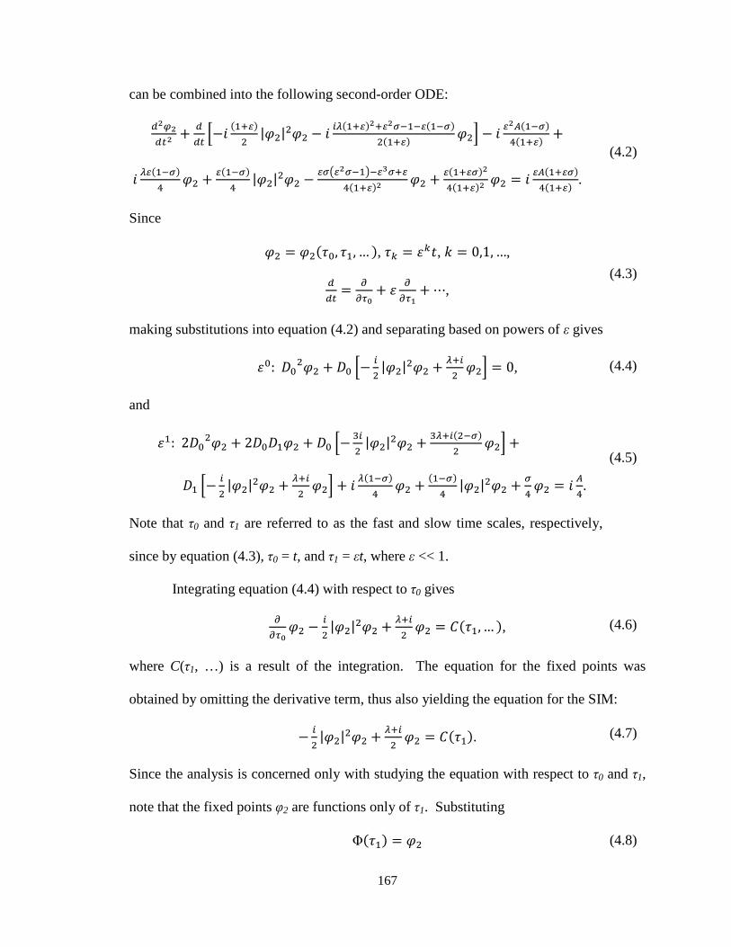
167

can be combined into the following second-order ODE:

n[[n[ nn || H [[ [ @ H @ @ || L[M\@ [ [@ [ @ .

Since

J4, J, … , Jb b, V 0,1, …,

nn 88» 88»m ¼,

making substitutions into equation (4.2) and separating based on powers of ε gives

4: /4 /4 || H 0,

and

: 2/4 2/4/ /4 || H / || H H @ @ || @ @.

Note that τ0 and τ1 are referred to as the fast and slow time scales, respectively,

since by equation (4.3), τ0 = t, and τ1 = εt, where ε << 1.

Integrating equation (4.4) with respect to τ0 gives

88» || H J, … ,

where C(τ1, …) is a result of the integration. The equation for the fixed points was

obtained by omitting the derivative term, thus also yielding the equation for the SIM:

|| H J .

Since the analysis is concerned only with studying the equation with respect to τ0 and τ1,

note that the fixed points φ2 are functions only of τ1. Substituting

ΦJ

(4.2)

(4.3)

(4.4)

(4.5)

(4.6)

(4.7)

(4.8)

168

and rearranging, equation (4.7) can be rewritten as

|Φ|Φ H Φ J .

Letting

ΦJ qJ o¾»m , and making the substitution, equation (4.9) becomes

qo¾ H qo¾ J , Through algebraic manipulations and taking the magnitude of equation (4.11), the

following relation was obtained:

qa 2q@ 1 q 4|J |.

Making the substitution,

J qJ £,

yields

2 1 4|J |.

Taking the derivative of the left hand side with respect to Z and setting equal to zero

gives

3 4 1 0.

The derivative has the following roots:

, ¨√H[ .

Since

qJ ~J ,

the positive values of N corresponding to the roots Z1,2 are given as

q, ¨√H[ ,

(4.10)

(4.11)

(4.12)

(4.13)

(4.14)

(4.15)

(4.16)

(4.17)

(4.18)

(4.9)

169

where N1 and N2 define the fold lines. Physically, fold lines correspond to the locations

on the SIM at which the trajectories of the SIM may jump between stable branches.

Equation (4.12) was used to generate the SIM projection on the (N, 4|C|2) plane

shown in Figure 4-1. As described by Starosvetsky and Gendelman (2008b), the fold

lines from equation (4.18) are plotted to show the locations for the jumps from one stable

branch of the SIM to another. Refer to Section 4.A.1.1 for detailed derivations of these

equations and Section 4.A.4.1 for the MATLAB code used for generation of Figure 4-1.

Figure 4-1. SIM projection for λ = 0.2 (linear damping) = stable; = unstable

0 0.2 0.4 0.6 0.8 1 1.2 1.4 1.60

0.02

0.04

0.06

0.08

0.1

0.12

0.14

0.16

0.18

0.2

N

4|C

|2

N1

N2

Nu

Nd

- - - - - - - -

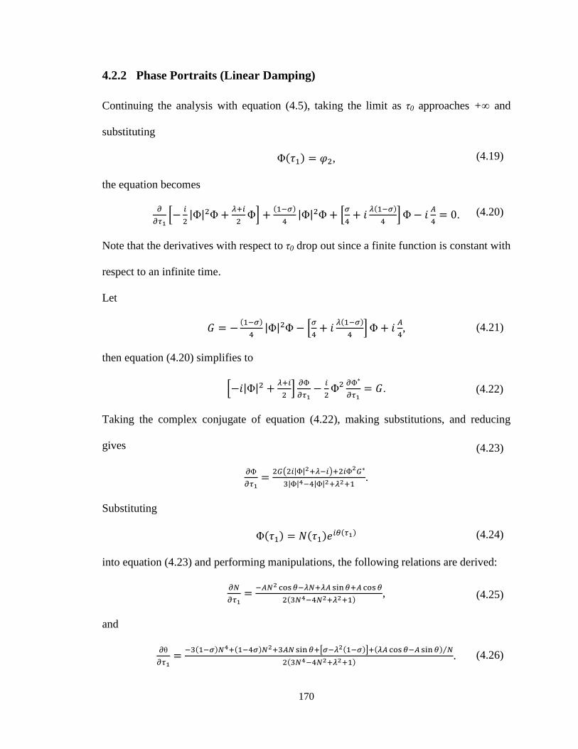
170

4.2.2 Phase Portraits (Linear Damping)

Continuing the analysis with equation (4.5), taking the limit as τ0 approaches +∞ and

substituting

ΦJ ,

the equation becomes

88»m |Φ|Φ H Φ @ |Φ|Φ @ H @ Φ @ 0.

Note that the derivatives with respect to τ0 drop out since a finite function is constant with

respect to an infinite time.

Let

¿ @ |Φ|Φ @ H @ Φ @,

then equation (4.20) simplifies to

|Φ| H 8Φ8»m Φ 8Φ¡8»m ¿.

Taking the complex conjugate of equation (4.22), making substitutions, and reducing

gives

8Φ8»m ÀL|Φ|[HMΦ[À¡|Φ|]@|Φ|[H[ .

Substituting

ΦJ qJ o¾»m into equation (4.23) and performing manipulations, the following relations are derived:

8Á8»m Á[ ÂÃÄ ¾HÁH ÄÅÆ ¾ ÂÃÄ ¾Á]@Á[H[ ,

and

8θ8»m Á]@ Á[Á ÄÅÆ ¾+H[ -H ÂÃÄ ¾ ÄÅÆ ¾ Á⁄Á]@Á[H[ .

(4.19)

(4.20)

(4.21)

(4.22)

(4.23)

(4.24)

(4.25)

(4.26)

171

Letting g(N) represent the denominator in equations (4.25) and (4.26), the fold lines occur

when g(N) = 0. Thus, the equations can be rescaled by g(N) to avoid singularities as

follows:

q& Aq cos q A sin A cos

and

θ& 31 ? q@ 1 4? q 3Aq sin

? 1 ? £ A cos A sin q⁄ .

Locations on the lower fold line at which θ is unchanging (and thus θ'=0) are denoted by

Θ1 and Θ2. The interval Θ1- Θ2 was derived in MATLAB by determining the values of θ

that satisfy these conditions. Refer to Section 4.A.4.2 for the code used for this

computation.

In addition, MATLAB was used to numerically integrate equations (4.27) and

(4.28) in order to generate the phase portraits shown in Figures 4-2, 4-3, and 4-4. Due to

the rescaling, N refers to N', and θ refers to ′ in these plots. The phase portraits were

generated for time up to five seconds. Refer to Section 4.A.1.2 for details on the equation

derivations and Section 4.A.4.4 for the MATLAB code. The phase portraits only show

stable trajectories on the SIM. Arrows denote the direction of the trajectories with

increasing time.

(4.27)

(4.28)

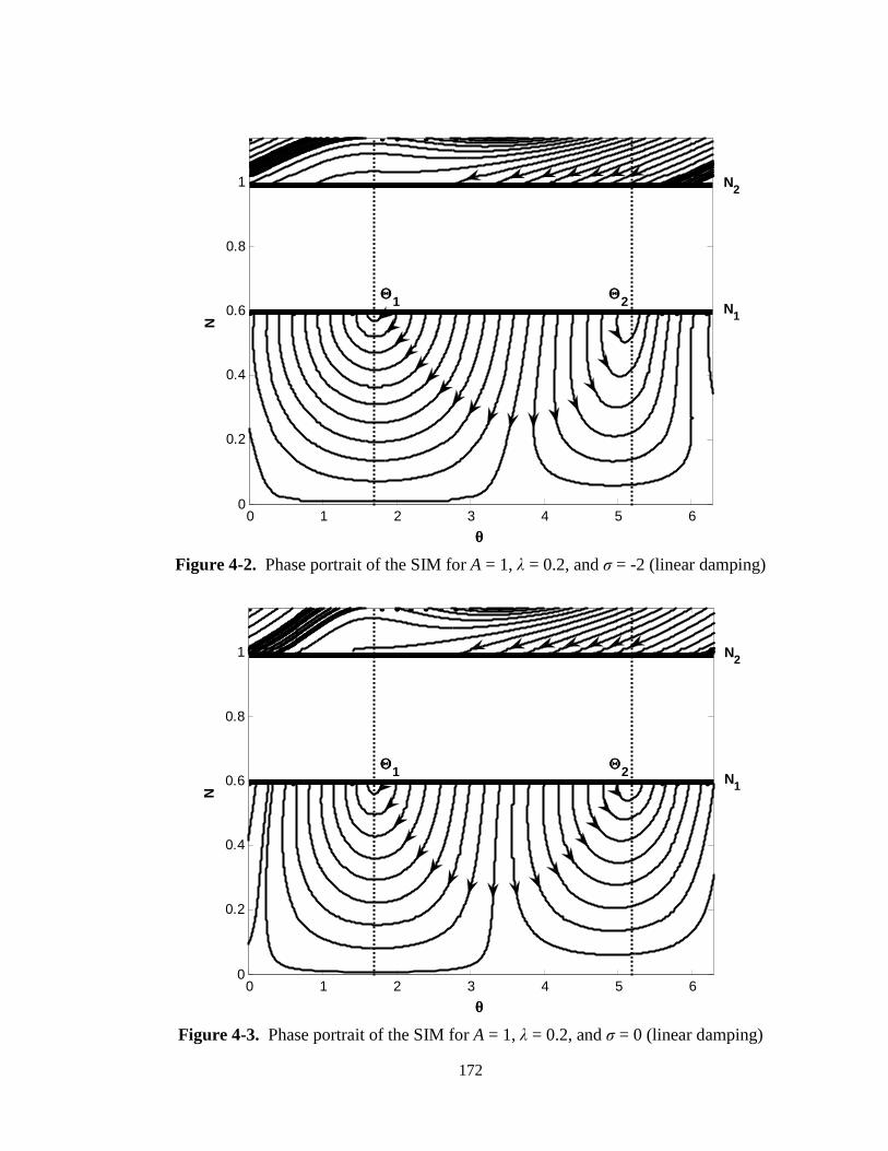
172

Figure 4-2. Phase portrait of the SIM for A = 1, λ = 0.2, and σ = -2 (linear damping)

Figure 4-3. Phase portrait of the SIM for A = 1, λ = 0.2, and σ = 0 (linear damping)

0 1 2 3 4 5 60

0.2

0.4

0.6

0.8

1

θθθθ

N

ΘΘΘΘ2ΘΘΘΘ1 N1

N2

0 1 2 3 4 5 60

0.2

0.4

0.6

0.8

1

θθθθ

N


N2

173

Figure 4-4. Phase portrait of the SIM for A = 1, λ = 0.2, and σ = 5 (linear damping)

4.2.3 1-D Mapping (Linear Damping)

Since C(τ1) is constant, equation (4.14) may be rewritten as

, 2, 1 , Ç,n 2Ç,n 1 Ç,n.

MATLAB was used to determine Zu,d (see Section 4.A.4.3 for the MATLAB code used).

Since one solution for Z1,2 (the fold lines) was already determined, the MATLAB code

returns the solutions that are not equivalent to Z1,2. Interpretation of the MATLAB output

gives

qÇ L1 √1 3M,

0 1 2 3 4 5 60

0.2

0.4

0.6

0.8

1

θθθθ

N


N2

(4.29)

(4.30)

174

and

qn L1 √1 3M.

From equation (4.11), the phase angle of the fixed point is found to be

J arg J tan LÁ[MH . Taking into account that C(τ1) is constant, manipulations between equations (4.30) and

(4.32) give the phase angle at Nu on the upper stable branch from the jump at N1:

Ç 4 tan H√H[cH[√H[. Additionally, equations (4.31) and (4.32) give the phase angle at Nd on the lower stable

branch from the jump at N2:

n 4 tan H√H[cH[√H[. Figures 4-5 through 4-9 were generated using MATLAB for varying values of σ. Refer

to Section 4.A.1.3 for details on the equation derivations, Section 4.A.3 for details on the

1-D map creation, and Section 4.A.4.4 for the MATLAB code. From varying σ and

observing when trajectories from the Θ1-Θ2 interval no longer returned, the SMR was

found to exist in the intervals of σ = [-5.07, 9.11] and σ = [9.73, 10.07].

(4.31)

(4.32)

(4.33)

(4.34)

175

Figure 4-5. 1-D map for A = 1, λ = 0.2, and σ = -2 (linear damping)

Figure 4-6. 1-D map for A = 1, λ = 0.2, and σ = 0 (linear damping)

-1.5 -1 -0.5 0 0.5 1 1.5 2

θθθθ

ΘΘΘΘ2 ΘΘΘΘ1

-1.5 -1 -0.5 0 0.5 1 1.5 2

θθθθ

ΘΘΘΘ2 ΘΘΘΘ1

176

Figure 4-7. 1-D map for A = 1, λ = 0.2, and σ = 5 (linear damping)

Figure 4-8. 1-D map for A = 1, λ = 0.2, and σ = -5.07 (linear damping)

-1.5 -1 -0.5 0 0.5 1 1.5 2

θθθθ

ΘΘΘΘ2 ΘΘΘΘ1

-1.5 -1 -0.5 0 0.5 1 1.5 2

θθθθ

ΘΘΘΘ2 ΘΘΘΘ1

177

Figure 4-9. 1-D map for A = 1, λ = 0.2, and σ = 9.11 (linear damping)

4.3 SMR Analysis for the System with Nonlinear Damping

4.3.1 Slow Invariant Manifold (SIM) Projection (Nonlinear Damping)

Equations (3.20),

and

1 ||

1 || ,

-1.5 -1 -0.5 0 0.5 1 1.5 2

θθθθ

ΘΘΘΘ2 ΘΘΘΘ1

(4.35)

178

can be combined into the following second-order ODE:

n[[n[ nn H@ ^ || [ [ @ H @a || [@ [ @ || L[M\@ [ @ .

Since

J4, J, … , Jb b, V 0,1, …,

nn 88» 88»m ¼,

making substitutions into equation (4.36) and separating based on powers of ε gives

4: /4 /4 H@ ^ || 0,

and

: 2/4 2/4/ /4 H@ ^ || / H@ ^ || H @a || @ @ || @ @.

Integrating equation (4.38) with respect to τ0 gives

88» H@ ^ || J, … ,


obtained by omitting the derivative term, thus also yielding the equation for the SIM:

H@ ^ || J .


note that the fixed points φ2 are functions only of τ1.

(4.36)

(4.38)

(4.39)

(4.40)

(4.37)

(4.41)

179

Substituting

ΦJ

and rearranging, equation (4.41) can be rewritten as

H@ ^ |Φ|Φ Φ J .

Letting

ΦJ qJ o¾»m , and making the substitution, equation (4.43) becomes

H@ ^ qo¾ qo¾ J ,

Through algebraic manipulations and taking the magnitude of equation (4.45), the

following relation was obtained:

9 16 qa 32q@ 16q 64|J |.


J qJ £,

yields

9 16 32 16 64|J |.


gives

39 16 64 16 0.


, ¨@√aµH[µH[@^ .

Since

qJ ~J ,

(4.42)

(4.43)

(4.44)

(4.45)

(4.46)

(4.47)

(4.48)

(4.49)

(4.50)

(4.51)

180

the positive values of N corresponding to the roots Z1,2 are given as

q, ¨@√aµH[µH[@^ ,

where N1 and N2 define the fold lines.

Equation (4.46) was used to generate the slow invariant manifold (SIM)

projection on the (N, 64|C|2) plane shown in Figure 4-10. As described by Starosvetsky

and Gendelman (2008b), the fold lines from equation (4.52) are plotted to show the

locations for the jumps from one stable branch of the SIM to another. Refer to Section

4.A.2.1 for detailed derivations of these equations and Section 4.A.4.5 for the MATLAB

code used for generation of Figure 4-10.

Figure 4-10. SIM projection for λ = 0.2 (nonlinear damping) = stable; = unstable

0 0.2 0.4 0.6 0.8 1 1.2 1.4 1.60

0.5

1

1.5

2

2.5

N

64|C

|2

N1

N2

Nu

Nd

- - - - - - - -

(4.52)

181

4.3.2 Phase Portraits (Nonlinear Damping)

Continuing the analysis with equation (4.39), taking the limit as τ0 approaches +∞ and

substituting

ΦJ ,


88»m Φ H@ ^ |Φ|Φ H@ a |Φ|Φ @ Φ @ 0.

Note that the derivatives with respect to τ0 drop out since a finite function is constant with

respect to an infinite time. Let

¿ H@ a |Φ|Φ @ Φ @,

then equation (4.54) simplifies to

H@ @ |Φ| 8Φ8»m H@ ^ Φ 8Φ¡8»m ¿.

Taking the complex conjugate of equation (4.56), making substitutions, and reducing

gives

8Φ8»m aÀ+H@ |Φ|[-^À¡H@ Φ[aa@|Φ|[H[a |Φ|] .

Substituting

ΦJ qJ o¾»m into equation (4.57) and performing manipulations, the following relations are derived:

8Á8»m HÁ\@H ÄÅÆ ¾@ ÂÃÄ ¾ Á[a ÂÃÄ ¾aa@Á[H[a Á]£ ,

and

8θ8»m LaµH[M Á]Ha @^£Á[@H ÂÃÄ ¾ ÄÅÆ ¾ ÁaaÄÅÆ ¾ /Áaa@Á[H[a Á]£ .

(4.53)

(4.54)

(4.55)

(4.56)

(4.57)

(4.58)

(4.59)

(4.60)

182

Letting g(N) represent the denominator in both differential equations, the fold lines occur


follows:

q′ 12q 4A3 sin 4 cos q 16A cos ,

and

′ 48 27 1 ? q@ 16 64? q

4A9 cos 12 sin q 16? 16A sin /q.

Locations on the lower fold line at which θ is unchanging (and thus θ'=0) are denoted by

Θ1 and Θ2. The interval Θ1- Θ2 was derived in MATLAB by determining the values of θ

that satisfy these conditions. Refer to Section 4.A.4.6 for the code used for this

computation.

In addition, MATLAB was used to numerically integrate equations (4.61) and

(4.62) in order to generate the phase portraits shown in Figures 4-11, 4-12, and 4-13.

Due to the rescaling, N refers to N', and θ refers to ′ in these plots. The phase portraits

were generated for time up to five seconds. Refer to Section 4.A.2.2 for details on the

equation derivations and Section 4.A.4.8 for the MATLAB code. The phase portraits

only show stable trajectories on the SIM. Arrows denote the direction of the trajectories

with increasing time.

(4.61)

(4.62)

183

Figure 4-11. Phase portrait of the SIM for A = 1, λ = 0.2, and σ = -4 (nonlinear damping)

Figure 4-12. Phase portrait of the SIM for A = 1, λ = 0.2, and σ = 0 (nonlinear damping)

0 1 2 3 4 5 60

0.2

0.4

0.6

0.8

1

θθθθ

N


N2

0 1 2 3 4 5 60

0.2

0.4

0.6

0.8

1

θθθθ

N


N2

184

Figure 4-13. Phase portrait of the SIM for A = 1, λ = 0.2, and σ = 4 (nonlinear damping)

4.3.3 1-D Mapping (Nonlinear Damping)

Since C(τ1) is constant, equation (4.48) may be rewritten as

9 16 , 32, 16, 9 16 Ç,n 32Ç,n 16Ç,n.




gives

qÇ ^√aµH[µH[@^ ,

0 1 2 3 4 5 60

0.2

0.4

0.6

0.8

1

θθθθ

N


N2

(4.63)

(4.64)

185

and

qn ^√aµH[µH[@^ .

From equation (4.45), the phase angle of the fixed point is found to be

J arg J tan @H ³ Á[ 1´. Taking into account that C(τ1) is constant, manipulations between equations (4.64) and

(4.66) give the phase angle at Nu on the upper stable branch from the jump at N1:

Ç 4 tan µHLH[aM√aµH[cH]aH[Lca√aµH[Ma@√aµH[ca. Additionally, equations (4.65) and (4.66) give the phase angle at Nd on the lower stable

branch from the jump at N2:

n 4 tan µHLH[aM√aµH[cH]aH[Lca√aµH[Ma@√aµH[ca. Figures 4-14 through 4-18 were generated using MATLAB. Refer to Section 4.A.2.3 for

details on the equation derivations, Section 4.A.3 for details on the 1-D map creation, and

Section 4.A.4.8 for the MATLAB code. From varying σ and observing when trajectories

from the Θ1-Θ2 interval no longer returned, the SMR was found to exist in the interval of

σ = [-7.17, 8.47].

(4.65)

(4.66)

(4.67)

(4.68)

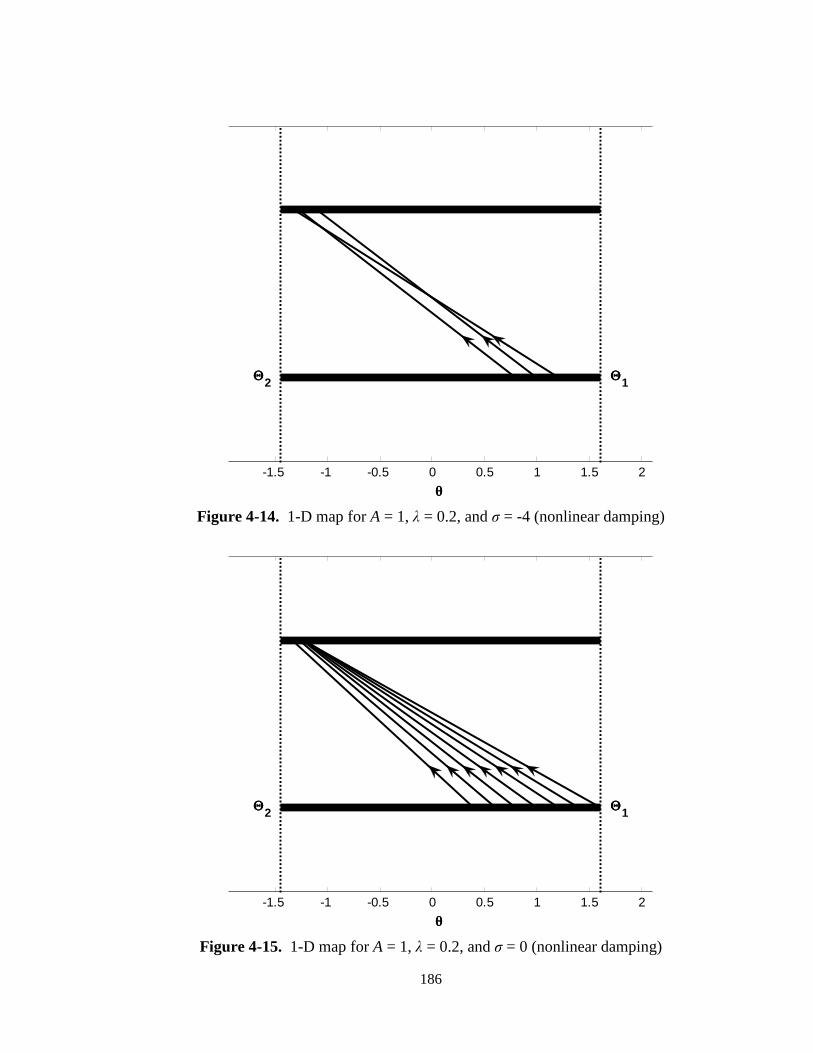
186

Figure 4-14. 1-D map for A = 1, λ = 0.2, and σ = -4 (nonlinear damping)

Figure 4-15. 1-D map for A = 1, λ = 0.2, and σ = 0 (nonlinear damping)

-1.5 -1 -0.5 0 0.5 1 1.5 2

θθθθ

ΘΘΘΘ2 ΘΘΘΘ1

-1.5 -1 -0.5 0 0.5 1 1.5 2

θθθθ

ΘΘΘΘ2 ΘΘΘΘ1

187

Figure 4-16. 1-D map for A = 1, λ = 0.2, and σ = 4 (nonlinear damping)

Figure 4-17. 1-D map for A = 1, λ = 0.2, and σ = -7.17 (nonlinear damping)

-1.5 -1 -0.5 0 0.5 1 1.5 2

θθθθ

ΘΘΘΘ2 ΘΘΘΘ1

-1.5 -1 -0.5 0 0.5 1 1.5 2

θθθθ

ΘΘΘΘ2 ΘΘΘΘ1

188

Figure 4-18. 1-D map for A = 1, λ = 0.2, and σ = 8.47 (nonlinear damping)

4.4 Discussion of Results for SMR

From observation of the preceding plots, there exist qualitative similarities between the

linearly and nonlinearly damped systems. First, comparison between the SIM projections

reveals that the values of N1, N2, Nu, and Nd in the linearly damped system are close to the

corresponding values in the nonlinearly damped system. Translating these values over to

the phase portraits shows locations of interest to the 1-D mapping. The fold lines are

depicted, separating stable and unstable regions. In all phase portraits, the trajectories

that leave the Θ1-Θ2 interval are evident with arrows denoting the direction of the

trajectory with increasing time. Note that in the neighborhood of σ = 0, the phase

portraits of the linearly and nonlinearly damped systems appear very similar. Qualitative

similarities are seen between the two systems for increasing magnitudes of σ as well.

-1.5 -1 -0.5 0 0.5 1 1.5 2

θθθθ

ΘΘΘΘ2 ΘΘΘΘ1

189

From observation of the 1-D maps, it is clear that varying σ has an effect on the

location of the return trajectories. When σ is increased or decreased beyond specific

values, the 1-D map can no longer be generated since the trajectories no longer return to

the Θ1- Θ2 interval. Hence, determining these threshold values gives a range of σ for the

existence of the SMR. Since σ is directly related to the frequency of the linear oscillator,

a frequency band for the SMR existence can be obtained. By equations (3.1) and (3.9),

the natural frequency of the linear oscillator in both linearly and nonlinearly damped

cases is given by

Ì=ÍÌÌ =ÍR ÌÌÍhhÌÌ =ÍR ÌQ R √1 ?.

Since the forcing frequency (1) in each case is very close to this natural frequency (~1),

due to ε << 1, the intervals of σ derived in this analysis also provide an approximate

range of forcing frequency for the occurrence of the SMR. For the linearly damped

system with ε = 0.05, the SMR exists for frequency ranges of [0.86, 1.21] and [1.22,

1.23]. Again using ε = 0.05, the SMR exists in the nonlinearly damped system for a

frequency range of [0.80, 1.19]. Thus, the SMR exists in both linearly and nonlinearly

damped systems near 1:1 resonance.

It should be noted that the results presented in this chapter are valid only for an

amplitude of A = 1. One may vary the amplitude to obtain results in other cases using the

same approach.

(4.69)

190

4.A Appendix

4.A.1 SMR Equation Derivations (Linear Damping)

4.A.1.1 Derivation of Equations Related to SIM Projection (Linear Damping)

Beginning with equations (3.11),

and

H 1 || .

the second equation can be rewritten as

H 1 || [ .

The equation can be reduced to

H 1 || L[M .

Solving for φ1 gives

H [ [ || [ .

Substituting into the first of equations (4.70) gives

nn H [ [ || [ H [ [ || [

H [ [ || [ .

(4.70)

(4.71)

(4.72)

(4.73)

(4.74)

191

This expression can be reduced to

n[[n[ nn H [ [ || [ [ H || \

[ H || L[M [ .

Since is not dependent on time, the derivative of this term with respect to time is

zero. Thus, this term may be removed from the bracketed expression corresponding to

the first derivative with respect to time. Taking this simplification into account and

further reducing the system gives

n[[n[ nn [ || H [[ [ H || L[M\

.

Taking into account that n[n , and reducing the system further gives

n[[n[ nn [ || H [[ [ H || L[M\

.

(4.75)

(4.76)

(4.77)

192

Again reducing the system yields

n[[n[ nn [ || H [[ [ H || L[M\

.

Multiplying by gives

n[[n[ nn || H [[ [ @ H @ @ || L[M\@ [ [@ [ @ .

Since

J4, J, … , Jb b, V 0,1, …,

nn 88» 88»m ¼ /4 / ¼,

and

n[n[ ³ 88» 88»m ¼ ´ /4 / ¼ ,

the equation can be rewritten as

/4 / ¼ /4 / ¼ || H [[ [ @ H @ @ || L[M\@ [

[@ [ @ .

(4.78)

(4.79)

(4.80)

(4.81)

(4.82)

193

Multiplying both sides by 1 gives

/4 / ¼ 1 /4 / ¼ g \ || H \³[ ´ [ @ H [@

[@ || L[M\@ [@ @ .

Expanding the equation and ignoring terms of and above gives

L/4 2/4/ ¼ M1 2 ¼ /4 / ¼ ¼ || H¼ ¼

H ¼@ ¼@ || ¼@ ¼@ ¼@ .

Reducing the equation gives

L/4 2/4/ ¼ M1 2 ¼ /4 / ¼ ¼ || H¼ ¼

H ¼@ ¼@ || ¼@ ¼@ .

Separating the equation based on powers of ε gives

4: /4 /4 2 || 2 0

and

: 2/4 2/4/ /4 || H / || H H @ @ || @ @.

Integrating the equation of order 4 with respect to τ0 gives

88» || H J, … ,

(4.83)

(4.84)

(4.85)

(4.86)

(4.88)

(4.87)

194


obtained by omitting the derivative term, thus yielding

|| H J .



ΦJ

and rearranging, the fixed point equation can be rewritten as

|Φ|Φ H Φ J .

Letting

ΦJ qJ o¾»m , and making the substitution, the equation becomes

qo¾ H qo¾ J , and thus

q H q o¾ J . Using the relation

o¾ cos sin

and substituting, the equation can be rewritten as

q H q cos sin J . Separating into real and imaginary parts gives

H q cos ³ q Á´ sin

H q sin ³ q Á´ cos J .

(4.89)

(4.90)

(4.91)

(4.92)

(4.93)

(4.94)

(4.95)

(4.96)

(4.97)

195


H q cos ³ q Á´ sin

H q sin ³ q Á´ cos |J |.

Expanding gives

H[@ q cos ³ q Á´ sin q ³ q Á´ sin cos

H[@ q sin ³ q Á´ cos q ³ q Á´ sin cos |J |.

Using trig identities, the equation becomes

H[@ q ³ q Á´ |J |.

Expanding the expression in parenthesis gives

H[@ q @ qa q@ @ q |J |.

Multiplying the equation by 4 gives

q qa 2q@ q 4|J |.

Finally, the equation is reduced to

qa 2q@ 1 q 4|J |.


J qJ £,

yields

2 1 4|J |.


gives

3 4 1 0.

(4.98)

(4.99)

(4.102)

(4.103)

(4.104)

(4.106)

(4.105)

(4.101)

(4.100)

196


, @äH[ a .

This equation reduces to

, ¨@H[ ,

which can be further simplified to

, ¨√H[ .

Since

qJ ~J ,

the positive values of N corresponding to the roots Z1,2 can be written as

q, ¨√H[ ,


4.A.1.2 Derivation of Equations Related to Phase Portraits (Linear Damping)

Continuing the analysis with the equation of O(ε1), taking the limit as τ0

approaches +∞ gives

/ || H H @

@ || @ @,

with D1 being replaced with the original notation. Note that the derivatives with respect

to τ0 drop out since a finite function is constant with respect to an infinite time. Reducing

and again substituting

ΦJ ,

(4.107)

(4.108)

(4.109)

(4.111)

(4.110)

(4.113)

(4.112)

197


88»m |Φ|Φ H Φ H @ Φ @ |Φ|Φ @ Φ @.

Simplifying yields

88»m |Φ|Φ H Φ @ |Φ|Φ @ H @ Φ @ 0.

Let

¿ @ |Φ|Φ @ H @ Φ @,

then

88»m |Φ|Φ H Φ ¿.

Distributing the derivative gives

|Φ| H 8Φ8»m Φ8|Φ|[8»m ¿.

But since

|Φ| ΦΦ¡, the expression can be rewritten as

|Φ| H 8Φ8»m Φ 88»m ΦΦ¡ ¿.


|Φ| H 8Φ8»m Φ Φ¡ 8Φ8»m Φ8Φ¡8»m ¿.


|Φ| H 8Φ8»m |Φ| 8Φ8»m Φ 8Φ¡8»m ¿.

Finally, the equation simplifies to

|Φ| H 8Φ8»m Φ 8Φ¡8»m ¿.

(4.115)

(4.114)

(4.117)

(4.116)

(4.119)

(4.118)

(4.121)

(4.120)

(4.123)

(4.122)

198

Taking the complex conjugate gives

|Φ| H 8Φ¡8»m Φ¡ 8Φ8»m ¿¡.

Solving for the complex conjugate derivative gives

8Φ¡8»m À¡:[Φ¡[ ÎΦÎÏm|Φ|[ÐÑ:[ .

Substituting into the expression above gives

|Φ| H 8Φ8»m Φ gÀ¡:[Φ¡[ ÎΦÎÏm|Φ|[ÐÑ:[ i ¿.

Multiplying the equation by ³|Φ| H ´ gives

³|Φ| H ´ ³|Φ| H ´ 8Φ8»m

Φ ³¿¡ Φ¡ 8Φ8»m´ ¿ ³|Φ| H ´.

Further manipulation yields

|Φ|@ |Φ| ³H H ´ H H @ 8Φ8»m Φ¿¡ @ ΦΦ¡ 8Φ8»m ¿ ³|Φ| H ´.

Simplifying gives

|Φ|@ |Φ| H[@ @ ΦΦ¡ 8Φ8»m Φ¿¡ ¿ ³|Φ| H ´.


+4|Φ|@ 4|Φ| 1 ΦΦ¡- 8Φ8»m

2Φ¿¡ 2¿2|Φ| .

Solving for the derivative term gives

8Φ8»m ÀL|Φ|[HMΦ[À¡@|Φ|]@|Φ|[H[Φ[Φ¡[.

(4.125)

(4.124)

(4.127)

(4.126)

(4.129)

(4.128)

(4.131)

(4.130)

199

Substituting in

|Φ|@ ΦΦ¡

and reducing gives

8Φ8»m ÀL|Φ|[HMΦ[À¡|Φ|]@|Φ|[H[ .

Since

ΦJ qJ o¾»m , the following can be written:

8Φ8»m 8Ò8»m o¾ qo¾ 8θ8»m. Thus,

8Φ8»m ³ 8Ò8»m q 8θ8»m´ o¾.

Setting equal to the expression above gives

³ 8Ò8»m q 8θ8»m´ o¾ ÀL|Φ|[HMΦ[À¡|Φ|]@|Φ|[H[ .

Again substituting

ΦJ qJ o¾»m gives

³ 8Ò8»m q 8θ8»m´ o¾ ÀLÁ[HMÁ[Í[:ÓÀ¡Á]@Á[H[ .

Moving the exponential term to the right hand side gives

8Á8»m q 8θ8»m ÀÍÑ:ÓLÁ[HMÁ[À¡Í:ÓÁ]@Á[H[ .

Substituting

ΦJ qJ o¾»m

(4.133)

(4.132)

(4.135)

(4.134)

(4.137)

(4.136)

(4.139)

(4.138)

(4.141)

(4.140)

200

into the expression for G gives

¿ @ qo¾ @ H @ qo¾ @.

Thus,

¿¡ @ qo¾ @ H @ qo¾ @.

Therefore,

¿o¾ @ q @ H @ q @ o¾,

and

¿¡o¾ @ q @ H @ q @ o¾.

Substituting into the differential equation gives

8Á8»m q 8θ8»m jmÑÔ ] Á\Ô]ÐmÑÔ ] ÁÕ]ÍÑ:ÓkLÁ[HMÁ]@Á[H[

Á[jmÑÔ ] Á\Ô]ÐmÑÔ ] ÁÕ]Í:ÓkÁ]@Á[H[ .

Manipulating the expression gives

8Á8»m q 8θ8»m jmÑÔ [ Á\Ô[ÐmÑÔ [ ÁÕ[ÍÑ:ÓkLÁ[HMÁ]@Á[H[

jmÑÔ [ Á_Ô[ÐmÑÔ [ Á\Õ[Í:ÓÁ[kÁ]@Á[H[ .

Reducing gives

8Á8»m q 8θ8»m Ö Á_H £Á\ÍÑ:ÓÁ[×Á]@Á[H[

jmÑÔ [ Á\Ô[ÐmÑÔ [ ÁÕ[ÍÑ:ÓkH Á]@Á[H[ jmÑÔ [ Á_Ô[ÐmÑÔ [ Á\Õ[Í:ÓÁ[kÁ]@Á[H[ .

(4.143)

(4.142)

(4.145)

(4.144)

(4.147)

(4.146)

(4.148)

201

Further simplification gives

8Á8»m q 8θ8»m jmÑÔ [ Á\Ô[ÐmÑÔ [ ÁÕ[ÍÑ:ÓkH Á]@Á[H[

j\mÑÔ [ Á_\Ô[ ÐmÑÔ [ Á\Á[³m[Í:ÓÍÑ:Ó´kÁ]@Á[H[ .

Multiplying out terms gives

8Á8»m q 8θ8»m jÐmÑÔ [ Á\HÔ[ÐmÑÔ [ ÁÐÕ[ ÍÑ:ÓkÁ]@Á[H[

jmÑÔ [ Á\Ô[ÐmÑÔ [ ÁÕ[ÍÑ:ÓkÁ]@Á[H[ j\mÑÔ [ Á_\Ô[ ÐmÑÔ [ Á\Á[³m[Í:ÓÍÑ:Ó´kÁ]@Á[H[ .

Further reductions give

8Á8»m q 8θ8»m ÖH Á\HH £ÁHÍÑ:Ó×Á]@Á[H[

Ö Á\H £ÁÍÑ:Ó×Á]@Á[H[ Ö Á_H £Á\Á[LÍ:ÓÍÑ:ÓM×Á]@Á[H[ .

Substituting

o¾ cos sin ,

and

o¾ cos sin

gives

8Á8»m q 8θ8»m ÖH Á\HH £ÁHÂÃÄ ¾ ÄÅÆ ¾ ×Á]@Á[H[

Ö Á\H £ÁÂÃÄ ¾ ÄÅÆ ¾ ×Á]@Á[H[

Ö Á_H £Á\Á[ ÂÃÄ ¾ ÄÅÆ ¾ ×Á]@Á[H[

(4.150)

(4.149)

(4.152)

(4.151)

(4.153)

(4.154)

202

Separating into real and imaginary parts gives

8Á8»m q 8θ8»m ÖH Á\HÁH ÄÅÆ ¾H Á ÂÃÄ ¾H Á\Á[ ÂÃÄ ¾×Á]@Á[H[ ÖH[ ÁH ÂÃÄ ¾ Á\Á ÄÅÆ ¾ Á_Á\Á[ ÄÅÆ ¾×Á]@Á[H[ .

Reducing gives

8Á8»m q 8θ8»m ÖH ÄÅÆ ¾HÁ ÂÃÄ ¾Á[ ÂÃÄ ¾×Á]@Á[H[

ÖH ÂÃÄ ¾@ Á\+H[ -Á ÄÅÆ ¾ Á_Á[ ÄÅÆ ¾×Á]@Á[H[ .

Equating real parts of the equation gives

8Á8»m H ÄÅÆ ¾HÁ ÂÃÄ ¾Á[ ÂÃÄ ¾Á]@Á[H[ ,

and equating imaginary parts gives

q 8θ8»m H ÂÃÄ ¾@ Á\+H[ -Á ÄÅÆ ¾ Á_Á[ ÄÅÆ ¾Á]@Á[H[ .

Final manipulations give

8Á8»m Á[ ÂÃÄ ¾HÁH ÄÅÆ ¾ ÂÃÄ ¾Á]@Á[H[ ,

and

8θ8»m Á]@ Á[Á ÄÅÆ ¾+H[ -H ÂÃÄ ¾ ÄÅÆ ¾ Á⁄Á]@Á[H[ .



follows:

q& Aq cos q A sin A cos

(4.155)

(4.156)

(4.157)

(4.158)

(4.159)

(4.160)

(4.161)

203

and

θ& 31 ? q@ 1 4? q

3Aq sin ? 1 ? £ A cos A sin q⁄ .

Phase portraits were generated using the rescaled equations. The folded singularities may

be obtained by setting θ& 0 and g(N) = 0, thus forcing the situation on the fold lines

with unchanging θ. Rewriting gives

θ& ?3q@ 4q 1 3q@ q 3Aq sin

A cos A sin q⁄ .

Since

wq 3q@ 4q 1,

setting g(N) = 0 and θ& 0 results in

3q@ q 3Aq sin Θ, LA cos Θ, A sin Θ,M q⁄ 0.

Rewriting gives

3q@ q 3Aq A/q sin Θ, LA cos Θ,M q⁄ 0.

Since

sin Θ, 1 cos Θ,,

the following may be written

3q@ q 3Aq A/q 1 cos Θ, LA cos Θ,M q⁄ 0.

MATLAB was used to solve for Θ and Θ (see Section 4.A.4.2).

(4.162)

(4.163)

(4.164)

(4.165)

(4.166)

(4.167)

(4.168)

204

4.A.1.3 Derivation of Equations Related to 1-D Mapping (Linear Damping)

Since C(τ1) is constant, equation

2 1 4|J |

may be rewritten as

, 2, 1 , Ç,n 2Ç,n 1 Ç,n.




gives

qÇ L1 √1 3M,

and

qn L1 √1 3M.

From

H q cos ³ q Á´ sin H q sin ³ q Á´ cos J ,

the argument of C(τ1) can be expressed as

arg J tan gÐ[Á ÄÅÆ ¾³m[Á\Ù[ ´ ÂÃÄ ¾Ð[Á ÂÃÄ ¾³m[Á\Ù[ ´ ÄÅÆ ¾i, which can be rewritten as

arg J tan HÁ ÄÅÆ ¾LÁ\ÁM ÂÃÄ ¾HÁ ÂÃÄ ¾Á\Á ÄÅÆ ¾.

(4.169)

(4.170)

(4.171)

(4.172)

(4.173)

(4.174)

(4.175)

205

Since the coefficient N is common to the numerator and denominator in the inverse

tangent expression, N may be factored out, leaving

arg J tan H ÄÅÆ ¾LÁ[M ÂÃÄ ¾H ÂÃÄ ¾Á[ ÄÅÆ ¾. Dividing the numerator and denominator in the inverse tangent expression by cos

gives

arg J tan Ú ÛÜÆ ¾LÙ[ÑmMÐLÙ[ÑmMÐ ÛÜÆ ¾Ý, which can be rewritten as

arg J tan Ú ÛÜÆ ¾LmÑÙ[MÐLmÑÙ[MÐ ÛÜÆ ¾Ý. Let

2 tan ,

and

2 LÁ[MH .

Then,

arg J tan *m*[*m*[. From the formula of the “sum and difference of two inverse circular functions” given by

Zwillinger (2003), the equation can be rewritten as

arg J tan 2 tan 2.

Thus,

arg J tantan tan LÁ[MH .

(4.176)

(4.177)

(4.178)

(4.179)

(4.182)

(4.181)

(4.180)

(4.183)

206

This equation can be reduced to

arg J J tan LÁ[MH . Finally, the following can be written:

J arg J tan LÁ[MH . Since

J qJ £,

the relation becomes

J arg J tan Þ»m H . Since C(τ1) is constant, the equation may be rewritten as

arg J 4,4 tan Þm,[H Ç,n tan Þß,àH . Thus,

Ç,n 4,4 tan Þm,[H tan Þß,àH . Let

# Þm,[H ,

and

# Þß,àH .

Then,

Ç,n 4,4 tan # tan #.

From the formula of the “sum and difference of two inverse circular functions” given by


Ç,n 4,4 tan !m![!m![.

(4.184)

(4.185)

(4.186)

(4.187)

(4.188)

(4.189)

(4.190)

(4.191)

(4.192)

(4.193)

207

Thus,

Ç,n 4,4 tan Ú ³mÑám,[Ð ´mÑáß,àÐ ³mÑám,[Ð ´mÑáß,àÐ Ý.

Reducing gives

Ç,n 4,4 tan g áß,àÑám,[Ð mÐ[LÞm,[MLÞß,àMi. The equation reduces to

Ç,n 4,4 tan LÞß,àÞm,[MHH[LÞm,[MLÞß,àM, and thus

Ç,n 4,4 tan LÁß,à[Ám,[[MHH[LÁm,[[MLÁß,à[M. Substituting in Nu and N1 gives

Ç 4 tan ¹[\L√H[M[ÑmÑ\Ð[\ ºHH[¹[ÑmÑ\Ð[\ º[\L√H[M.

Reducing gives

Ç 4 tan H√H[H[[\L√H[M[ÑmÑ\Ð[\ [\L√H[M¹[ÑmÑ\Ð[\ º.


Ç 4 tan g H√H[H[]\m\√H[[âL√H[ML√H[Mi. Simplification leads to

Ç 4 tan g H√H[H[m\m\√H[[âL√H[H[Mi.

(4.194)

(4.195)

(4.196)

(4.197)

(4.198)

(4.199)

(4.200)

(4.201)

208

The equation can be rewritten as

Ç 4 tan H√H[H[√H[L√H[H[M. Simplifying gives

Ç 4 tan H√H[cH[√H[. Substituting in Nd and N2 gives

n 4 tan ¹[\L√H[M[ãmÑ\Ð[\ ºHH[¹[ãmÑ\Ð[\ º[\L√H[M.

Reducing gives

n 4 tan H√H[H[[\L√H[M[ãmÑ\Ð[\ [\L√H[M¹[ãmÑ\Ð[\ º.


n 4 tan g H√H[H[]\m\√H[[âL√H[ML√H[Mi. Simplification leads to

n 4 tan g H√H[H[m\m\√H[[âL√H[H[Mi. The equation can be rewritten as

n 4 tan H√H[H[√H[L√H[H[M. Simplifying gives

n 4 tan H√H[cH[√H[.

(4.202)

(4.203)

(4.204)

(4.205)

(4.206)

(4.207)

(4.208)

(4.209)

209

Using the properties of inverse tangent as given by Zwillinger (2003),

n 4 tan H√H[cH[√H[. 4.A.2 SMR Equation Derivations (Nonlinear Damping)

4.A.2.1 Derivation of Equations Related to SIM Projection (Nonlinear Damping)

Beginning with equations (3.20),

and

1 ||

1 || ,

the second equation can be rewritten as

1 ||

1 || [ .


1 ||

1 || L[M .

Solving for φ1 gives

H [@ || [ || [ .

(4.210)

(4.211)

(4.213)

(4.212)

(4.214)

210

Substituting into the first of equations (4.211) gives

nn H [@ || [ || [ H [@ || [ ||

[ H [@ || [ || [ .

This expression can be reduced to

n[[n[ nn H [@ || [ || [ [ H ^ || ||

\ [ [ H ^ || || L[M [ .

Since is not dependent on time, the derivative of this term with respect to time is

zero. Thus, this term may be removed from the bracketed expression corresponding to

the first derivative with respect to time. Taking this simplification into account and

further reducing the system gives

n[[n[ nn H@ [@ || [

[ H @ ^ || || L[M\ .

(4.215)

(4.216)

(4.217)

211

Taking into account that n[n and reducing the system further gives

n[[n[ nn H@ [@ || [ [ H @ ^ || || L[M\ .

Again reducing the system yields

n[[n[ nn H@ [@ || [

[ H @ ^ || || L[M\ .

Multiplying by gives

n[[n[ nn H@ ^ || [ [ @ H @a || [@ [ @ ||

L[M\@ [ @ .

Since

J4, J, … , Jb b, V 0,1, …,

nn 88» 88»m ¼ /4 / ¼,

and

n[n[ ³ 88» 88»m ¼ ´ /4 / ¼ ,

(4.218)

(4.219)

(4.220)

(4.221)

(4.222)

212

the equation can be rewritten as

/4 / ¼ /4 / ¼ H@ ^ || [ [ @ H @a || [@ [

@ || L[M\@ [ @ .

Multiplying both sides by 1 gives

/4 / ¼ 1 /4 / ¼ H@ \^ || + [- [ @ H @£ [a || [@ [@ || L[M\@ @ .

Expanding the equation and ignoring terms of and above gives

L/4 2/4/ ¼ M1 2 ¼ /4 / ¼ H@ ¼ ^ || ¼

H @£¼a || ¼@ ¼@ || ¼@ ¼@ .

Separating the equation based on powers of ε gives

4: /4 /4 H@ ^ || 0

and

: 2/4 2/4/ /4 H@ ^ ||

/ H@ ^ || H @a || @

@ || @ @.

(4.223)

(4.224)

(4.225)

(4.226)

(4.227)

213

Integrating the equation of order 4 with respect to τ0 gives

88» H@ ^ || J, … ,


obtained by omitting the derivative term, thus yielding

H@ ^ || J .



ΦJ

and rearranging, the fixed point equation can be rewritten as

H@ ^ |Φ|Φ Φ J .

Letting

ΦJ qJ o¾»m , and making the substitution, the equation becomes

H@ ^ qo¾ qo¾ J ,

and thus

H@ ^ q q o¾ J .

Using the relation

o¾ cos sin

and substituting, the equation can be rewritten as

H@ ^ q q cos sin J .

(4.228)

(4.229)

(4.230)

(4.231)

(4.232)

(4.233)

(4.234)

(4.235)

(4.236)

214


H ÂÃÄ ¾@ ÄÅÆ ¾ ^ q Á sin H ÄÅÆ ¾@ ÂÃÄ ¾ ^ q Á cos J .


H ÂÃÄ ¾@ ÄÅÆ ¾ ^ q Á sin H ÄÅÆ ¾@ ÂÃÄ ¾ ^ q Á cos |J |.

Expanding gives

H ÂÃÄ ¾@ ÄÅÆ ¾ [a@ qa H ÂÃÄ ¾@ ÄÅÆ ¾ ÄÅÆ ¾^ q@ Á[@ sin H ÄÅÆ ¾@ ÂÃÄ ¾ [a@ qa H ÄÅÆ ¾@ ÂÃÄ ¾ ÂÃÄ ¾^ q@ Á[@ cos |J |.

Further expansion and reduction gives

H[ ÂÃÄ[ ¾@H ÂÃÄ ¾ ÄÅÆ ¾a ÄÅÆ[ ¾a@ qa ÄÅÆ[ ¾ q@ Á[@ sin H[ ÄÅÆ[ ¾@H ÂÃÄ ¾ ÄÅÆ ¾a ÂÃÄ[ ¾a@ qa ÂÃÄ[ ¾ q@ Á[@ cos |J |.


H[LÄÅÆ[ ¾ÂÃÄ[ ¾MaLÄÅÆ[ ¾ÂÃÄ[ ¾Ma@ qa Á] sin cos

Á[@ sin cos |J |.

Using trig identities, the equation becomes

H[aa@ qa Á] Á[@ |J |.

Eliminating the denominators gives

9 16 qa 32q@ 16q 64|J |.

Making the substitution, J qJ £,

yields

9 16 32 16 64|J |.

(4.237)

(4.238)

(4.239)

(4.240)

(4.241)

(4.242)

(4.243)

(4.244)

(4.245)

215


gives

39 16 64 16 0.


, a@¨@4aH[a aH[a .

Reducing begins with

, a@¨√@4a4µµ^H[aH[a .

Simplifying gives

, a@¨√4@µ^H[aH[a ,

which then becomes

, a@ä@aµH[ aH[a .

The equation gives

, a@¨^√aµH[aH[a ,

which can be further reduced to

, ¨@√aµH[H[a .

Finally, the equation becomes

, ¨@√aµH[µH[@^ .

Since

qJ ~J ,

(4.246)

(4.247)

(4.248)

(4.249)

(4.250)

(4.251)

(4.252)

(4.253)

(4.254)

216

the positive values of N corresponding to the roots Z1,2 can be written as

q, ¨@√aµH[µH[@^ ,


4.A.2.2 Derivation of Equations Related to Phase Portraits (Nonlinear Damping)

Continuing the analysis with the equation of O(ε1), taking the limit as τ0

approaches +∞ gives

88»m H@ ^ || H @a ||

@ @ || @ @,

with D1 being replaced with the original notation. Note that the derivatives with respect

to τ0 drop out since a finite function is constant with respect to an infinite time. Reducing

and again substituting

ΦJ ,


88»m Φ H@ ^ |Φ|Φ H @a |Φ|Φ @ |Φ|Φ @ Φ @.

Simplifying yields

88»m Φ H@ ^ |Φ|Φ H a |Φ|Φ @ |Φ|Φ

@ |Φ|Φ @ Φ @.

Continuing with the simplification yields

88»m Φ H@ ^ |Φ|Φ H a |Φ|Φ @ |Φ|Φ @ Φ @,

(4.255)

(4.256)

(4.257)

(4.258)

(4.259)

(4.260)

217

which reduces further to

88»m Φ H@ ^ |Φ|Φ H@ a |Φ|Φ @ Φ @ 0.

Let

¿ H@ a |Φ|Φ @ Φ @,

then

88»m Φ H@ ^ |Φ|Φ ¿.


H@ ^ |Φ| 8Φ8»m H@ ^ Φ8|Φ|[8»m ¿.

But since

|Φ| ΦΦ¡, the expression can be rewritten as

H@ ^ |Φ| 8Φ8»m H@ ^ Φ 88»m ΦΦ¡ ¿.


H@ ^ |Φ| 8Φ8»m H@ ^ Φ Φ¡ 8Φ8»m Φ8Φ¡8»m ¿.


H@ ^ |Φ| 8Φ8»m H@ ^ |Φ| 8Φ8»m H@ ^ Φ 8Φ¡8»m ¿.

Finally, the equation simplifies to

H@ @ |Φ| 8Φ8»m H@ ^ Φ 8Φ¡8»m ¿.

Taking the complex conjugate gives

H@ @ |Φ| 8Φ¡8»m H@ ^ Φ¡ 8Φ8»m ¿¡.

(4.261)

(4.262)

(4.263)

(4.264)

(4.265)

(4.266)

(4.267)

(4.268)

(4.269)

(4.270)

218

Solving for the complex conjugate derivative gives

8Φ¡8»m À¡\Ðã]: ä Φ¡[ ÎΦÎÏm:[\Ðã]: ] |Φ|[ .

Substituting into the expression above gives

H@ @ |Φ| 8Φ8»m H@ ^ Φ gÀ¡\Ðã]: ä Φ¡[ ÎΦÎÏm:[\Ðã]: ] |Φ|[ i ¿.


4 23 4 |Φ|£ 8Φ8»m 3 4 Φ gÀ¡\Ðã]: ä Φ¡[ ÎΦÎÏm:[\Ðã]: ] |Φ|[ i 8¿.

Simplifying the fraction in the bracketed term gives

4 23 4 |Φ|£ 8Φ8»m 3 4 Φ g^À¡H@ Φ¡[ ÎΦÎÏm@H@ |Φ|[ i 8¿.

Further manipulation yields

N4 23 4 |Φ| H@ H@ Φ[Φ¡[@H@ |Φ|[ f 8Φ8»m ^À¡H@ Φ[@H@ |Φ|[ 8¿.

Solving for the derivative term gives

8Φ8»m ^À äå¡\ÐÑ]: Φ[Ñ]:ã[\Ðã]: |Φ|[@H@ |Φ|[g\ÐÑ]: \Ðã]: Φ[Φ¡[Ñ]:ã[\Ðã]: |Φ|[ i.

Simplifying gives

8Φ8»m ^À+@H@ |Φ|[-^À¡H@ Φ[@H@ |Φ|[£@H@ |Φ|[£H@ H@ Φ[Φ¡[. Expanding the terms in the denominator gives

8Φ8»m ^À+@H@ |Φ|[-^À¡H@ Φ[a^H@ |Φ|[^H@ |Φ|[@H[a |Φ|]H[a Φ[Φ¡[. Substituting in

|Φ|@ ΦΦ¡

(4.271)

(4.272)

(4.273)

(4.274)

(4.275)

(4.276)

(4.277)

(4.278)

(4.279)

219

and reducing gives

8Φ8»m aÀ+H@ |Φ|[-^À¡H@ Φ[a^H@ |Φ|[^H@ |Φ|[H[a |Φ|].

Simplifying the denominator gives

8Φ8»m aÀ+H@ |Φ|[-^À¡H@ Φ[a^|Φ|[H@H@ H[a |Φ|]. Finally, the expression can be written as

8Φ8»m aÀ+H@ |Φ|[-^À¡H@ Φ[aa@|Φ|[H[a |Φ|] .

Since

ΦJ qJ o¾»m , the following can be written:

8Φ8»m 8Ò8»m o¾ qo¾ 8θ8»m. Thus,

8Φ8»m ³ 8Ò8»m q 8θ8»m´ o¾.

Setting equal to the expression above gives

³ 8Ò8»m q 8θ8»m´ o¾ aÀ+H@ |Φ|[-^À¡H@ Φ[aa@|Φ|[H[a |Φ|] .

Again substituting

ΦJ qJ o¾»m gives

³ 8Ò8»m q 8θ8»m´ o¾ aÀ+H@ Á[-^À¡H@ Á[Í[:Óaa@Á[H[a Á] .

Moving the exponential term to the right hand side gives

8Á8»m q 8θ8»m aÀÍÑ:Ó+H@ Á[-^À¡Í:ÓH@ Á[aa@Á[H[a Á] .

(4.280)

(4.281)

(4.282)

(4.283)

(4.284)

(4.285)

(4.286)

(4.287)

(4.288)

(4.289)

220

Substituting

ΦJ qJ o¾»m into the expression for G gives

¿ H@ a qo¾ @ qo¾ @.

Thus,

¿¡ H@ a qo¾ @ qo¾ @.

Therefore,

¿o¾ H@ a q @ q @ o¾,

and

¿¡o¾ H@ a q @ q @ o¾.

Substituting into the differential equation gives

8Á8»m q 8θ8»m a\Ð:ã] mÑÔ mæ Á\Ô]ÁÕ]ÍÑ:Ó+H@ Á[-^Ñ\Ð:ã] mÑÔ mæ Á\Ô]ÁÕ]Í:ÓH@ Á[aa@Á[H[a Á] .

Manipulating the expression gives

8Á8»m q 8θ8»m a[:\Ð:ã] mÑÔ mæ Á\Ô]ÁÕ[ÍÑ:Ó\Ð:ã] \Ðã]: mÑÔ mæ Á_Ô\Ðã]: ] Á\Õ\Ðã]: ] ÍÑ:ÓÁ[aa@Á[H[a Á] ^Ñ\Ð:ã] \ÐÑ]: mÑÔ mæ Á\Ô\ÐÑ]: ] ÁÕ\ÐÑ]: ] Í:ÓÁ[aa@Á[H[a Á] .

(4.290)

(4.291)

(4.292)

(4.293)

(4.294)

(4.295)

(4.296)

221

Reducing gives

8Á8»m q 8θ8»m +H@ Á\^Á^ÍÑ:ÓH@ H@ Á_@H@ Á\@H@ ÍÑ:ÓÁ[-aa@Á[H[a Á] Ñ\Ð:ã] \ÐÑ]: mÑÔ [ Á\H@ ÁH@ Í:ÓÁ[aa@Á[H[a Á] .

Further simplification gives

8Á8»m q 8θ8»m +H@ Á\^Á^ÍÑ:ÓH@ H@ Á_@H@ Á\@H@ ÍÑ:ÓÁ[-aa@Á[H[a Á] +H@ H@ Á\@H@ Á@H@ Í:Ó-Á[aa@Á[H[a Á]£ .

Multiplying out terms gives

8Á8»m q 8θ8»m +aH^ Á\^Á^ÍÑ:ÓLaH[M Á_@H@ Á\@H@ ÍÑ:ÓÁ[-aa@Á[H[a Á] +LH[aM Á\@H@ Á@H@ Í:Ó-Á[aa@Á[H[a Á]£ .

Continuing with reducing the equation gives

8Á8»m q 8θ8»m +aH^ Á\^Á^ÍÑ:ÓLaH[M Á_@H@ Á\@H@ ÍÑ:ÓÁ[-aa@Á[H[a Á]£ +LH[aM Á_@H@ Á\@H@ Í:ÓÁ[-aa@Á[H[a Á]£ .

Substituting

o¾ cos sin

(4.297)

(4.298)

(4.299)

(4.300)

(4.301)

222

and

o¾ cos sin

gives

8Á8»m q 8θ8»m +aH^ Á\^Á^ÂÃÄ ¾ ÄÅÆ ¾ LaH[M Á_@H@ Á\@H@ ÂÃÄ ¾ ÄÅÆ ¾ Á[-aa@Á[H[a Á]£ +LH[aM Á_@H@ Á\@H@ ÂÃÄ ¾ ÄÅÆ ¾ Á[-aa@Á[H[a Á]£ .

Reducing again yields

8Á8»m q 8θ8»m aH^ Á\^Á^ÂÃÄ ¾ ÄÅÆ ¾ aH[ Á_@H@ Á\@H ÂÃÄ ¾H ÄÅÆ ¾@ ÂÃÄ ¾@ ÄÅÆ ¾ Á[£aa@Á[H[a Á]£ H[a Á_@H@ Á\@H ÂÃÄ ¾H ÄÅÆ ¾@ ÂÃÄ ¾@ ÄÅÆ ¾ Á[£aa@Á[H[a Á]£ .

Distributing the 2 in the numerator leads to

8Á8»m q 8θ8»m Ha Á\aÁaÂÃÄ ¾ ÄÅÆ ¾ ^H[ Á_@aH^ Á\@aH ÂÃÄ ¾aH ÄÅÆ ¾^ ÂÃÄ ¾^ ÄÅÆ ¾ Á[£aa@Á[H[a Á]£ H[a Á_@H@ Á\@H ÂÃÄ ¾H ÄÅÆ ¾@ ÂÃÄ ¾@ ÄÅÆ ¾ Á[£aa@Á[H[a Á]£ .

Simplifying gives

8Á8»m q 8θ8»m Ha Á\aÁaÂÃÄ ¾ ÄÅÆ ¾ @^µH[ Á_@H Á\@H ÂÃÄ ¾H ÄÅÆ ¾@ ÂÃÄ ¾ ÄÅÆ ¾ Á[£aa@Á[H[a Á]£ .


8Á8»m q 8θ8»m +H Á\a ÂÃÄ ¾HÁ\@H ÄÅÆ ¾@ ÂÃÄ ¾ Á[-aa@Á[H[a Á]£ +a Á\aÁa ÄÅÆ ¾L@^µH[M Á_@^Á\@H ÂÃÄ ¾ ÄÅÆ ¾ Á[-aa@Á[H[a Á]£ .

(4.302)

(4.303)

(4.304)

(4.305)

(4.306)

(4.307)

223

Equating real parts of the equation gives

8Á8»m H Á\a ÂÃÄ ¾HÁ\@H ÄÅÆ ¾@ ÂÃÄ ¾ Á[aa@Á[H[a Á]£ ,

and equating imaginary parts gives

q 8θ8»m a Á\aÁa ÄÅÆ ¾L@^µH[M Á_@^Á\@H ÂÃÄ ¾ ÄÅÆ ¾ Á[Áaa@Á[H[a Á]£ .

Final simplifications give

8Á8»m HÁ\@H ÄÅÆ ¾@ ÂÃÄ ¾ Á[a ÂÃÄ ¾aa@Á[H[a Á]£ ,

and

8θ8»m L@^µH[M Á]aa@ Á[@H ÂÃÄ ¾ ÄÅÆ ¾ Áaa ÄÅÆ ¾ /Áaa@Á[H[a Á]£ .


when g(N) = 0. Thus, the equations can be rescaled by g(N) to avoid infinite responses as

follows:

q′ 12q 4A3 sin 4 cos q 16A cos ,

and

θ′ 48 27 1 ? q@ 16 64? q

4A9 cos 12 sin q 16? 16A sin /q.

Phase portraits were generated using the rescaled equations. The folded singularities may

be obtained by setting θ& 0 and g(N) = 0, thus forcing the situation on the fold lines

with unchanging θ. Rewriting gives

θ′ ?48 27 q@ 64q 16£ 48 27 q@

16q 4A9 cos 12 sin q 16A sin /q.

Since

wq 48 27 q@ 64q 16,

(4.308)

(4.309)

(4.310)

(4.311)

(4.312)

(4.314)

(4.313)

(4.315)

224

setting g(N) = 0 and θ& 0 results in

48 27 q@ 16q 4AL9 cos Θ, 12 sin Θ,Mq

L16A sin Θ,M/q 0.

Rewriting gives

48 27 q@ 16q 36Aq cos Θ,

48Aq 16A/q sin Θ, 0.

Since

sin Θ, 1 cos Θ,,

the following may be written

48 27 q@ 16q 36Aq cos

48Aq 16A/q 1 cos Θ, 0.

MATLAB was used to solve for Θ and Θ (see Section 4.A.4.6).

4.A.2.3 Derivation of Equations Related to 1-D Mapping (Nonlinear Damping)

Since C(τ1) is constant, equation

9 16 32 16 64|J |

may be rewritten as

9 16 , 32, 16,

9 16 Ç,n 32Ç,n 16Ç,n.



(4.316)

(4.317)

(4.318)

(4.319)

(4.320)

(4.321)

225


gives

qÇ ^√aµH[µH[@^ ,

and

qn ^√aµH[µH[@^ .

From

g3 cos 4 sin 8 q q2 sin i

H ÄÅÆ ¾@ ÂÃÄ ¾ ^ q Á cos J ,

the argument of C(τ1) can be expressed as

arg J tan g\Ð çèé ÓÑ] êëç Ó ä Á\Ù[ ÂÃÄ ¾\Ð êëç Óã] çèé Ó ä Á\Ù[ ÄÅÆ ¾i, which can be rewritten as

arg J tan H ÄÅÆ ¾@ ÂÃÄ ¾ Á\@Á ÂÃÄ ¾H ÂÃÄ ¾@ ÄÅÆ ¾ Á\@Á ÄÅÆ ¾. Since the coefficient N is common to the numerator and denominator in the inverse

tangent expression, N may be factored out, leaving

arg J tan H ÄÅÆ ¾@ ÂÃÄ ¾ Á[@ ÂÃÄ ¾H ÂÃÄ ¾@ ÄÅÆ ¾ Á[@ ÄÅÆ ¾. Dividing the numerator and denominator in the inverse tangent expression by cos gives

arg J tan H ÛÜÆ ¾@ Á[@H@ ÛÜÆ ¾ Á[@ ÛÜÆ ¾, which can be rewritten as

arg J tan g H ÛÜÆ ¾@ ]Ù[H@ ÛÜÆ ¾ ]Ù[ ÛÜÆ ¾i.

(4.322)

(4.323)

(4.324)

(4.325)

(4.326)

(4.327)

(4.328)

(4.329)

226

Reducing gives

arg J tan gH ÛÜÆ ¾@³ mÙ[´H@³ mÙ[´ ÛÜÆ ¾i. Dividing the numerator and denominator by 3 gives

arg J tan g ÛÜÆ ¾ ]\Ð³ mÙ[´ ]\Ð³ mÙ[´ ÛÜÆ ¾i. Let

2 tan ,

and

2 @H ³ Á[ 1´.

Then,

arg J tan *m*[*m*[. From the formula of the “sum and difference of two inverse circular functions” given by


arg J tan 2 tan 2.

Thus,

arg J tantan tan @H ³ Á[ 1´. The equation can be reduced to

arg J J tan @H ³ Á[ 1´. Finally, the following can be written:

J arg J tan @H ³ Á[ 1´. Since

J qJ £,

(4.330)

(4.331)

(4.332)

(4.333)

(4.334)

(4.335)

(4.336)

(4.337)

(4.338)

(4.339)

227

the relation becomes

J arg J tan @H ³ Þ»m 1´. Since C(τ1) is constant, the equation may be written as

arg J 4,4 tan @H Þm,[ 1 Ç,n tan @H Þß,à 1. Thus,

Ç,n 4,4 tan @H Þm,[ 1 tan @H Þß,à 1. Let

# @H Þm,[ 1,

and

# @H Þß,à 1.

Then,

Ç,n 4,4 tan # tan #.

From the formula of the “sum and difference of two inverse circular functions” given by


Ç,n 4,4 tan !m![!m![. Thus,

Ç,n 4,4 tan Ú ]\Ð mám,[ ]\Ð máß,à ]\Ð mám,[ ]\Ð máß,àÝ.

(4.340)

(4.341)

(4.342)

(4.343)

(4.344)

(4.345)

(4.346)

(4.347)

228

Reducing gives

Ç,n 4,4 tan Ú ]\Ð mám,[ máß,à mæâÐ[ mám,[ máß,àÝ.

Multiplying the numerator and denominator by 9 gives

Ç,n 4,4 tan Ú H mám,[ máß,àH[a mám,[ máß,àÝ,

and thus

Ç,n 4,4 tan H¹ mÙm,[[ mÙß,à[ºH[a¹ mÙm,[[º¹ mÙß,à[º.

Substituting in Nu and N1 gives

Ç 4 tanìííííî Hï m\[Ñ]mæÑ[ðÐ[[ðÐ[ã]ä

m\[ãämæÑ[ðÐ[[ðÐ[ã]äñ

H[aï m\[Ñ]mæÑ[ðÐ[[ðÐ[ã]äñï m\[ãämæÑ[ðÐ[[ðÐ[ã]ä

ñòóóóóô,

which becomes

Ç 4 tan H [ðÐ[ã]ä\[Ñ]mæÑ[ðÐ[ [ðÐ[ã]ä\[ãämæÑ[ðÐ[H[a [ðÐ[ã]ä\[Ñ]mæÑ[ðÐ[ [ðÐ[ã]ä\[ãämæÑ[ðÐ[.


Ç 4 tan H [ðÐ[ã]ä\[Ñ]mæÑ[ðÐ[ [ðÐ[ã]ä\[ãämæÑ[ðÐ[H[a a [ðÐ[ã]ä\[Ñ]mæÑ[ðÐ[ [ðÐ[ã]ä\[ãämæÑ[ðÐ[ [ðÐ[ã]ä\[Ñ]mæÑ[ðÐ[ [ðÐ[ã]ä\[ãämæÑ[ðÐ[.

Multiplying the numerator and denominator by L32 4√16 27ML32 8√16 27 gives

Ç 4 tan H+LµH[@^ML^√aµH[MLµH[@^ML@√aµH[M-H[a L@√aµH[ML^√aµH[Ma+µH[@^ [µH[@^ L^√aµH[MµH[@^ L@√aµH[M-.

(4.348)

(4.349)

(4.350)

(4.351)

(4.352)

(4.353)

(4.354)

229

Reducing gives

Ç 4 tan HLµH[@^M+L^√aµH[ML@√aµH[M-H[a L@√aµH[ML^√aµH[MaµH[@^ [aµH[@^ +L^√aµH[ML@√aµH[M-. Continuing with the reduction yields

Ç 4 tan HµH[@^ L√aµH[MH[a L@√aµH[ML^√aµH[MaµH[@^ [aµH[@^ La@@√aµH[M, which leads to

Ç 4 tan @@HµH[@^ √aµH[H[a +4@^√aµH[aµH[ -aµH[@^ [aµH[@^ La@@√aµH[M. Simplifying gives

Ç 4 tan @@HµH[@^ √aµH[H[a +4@^√aµH[câ@H[-aµH[@^ [aµH[@^ La@@√aµH[M, becoming

Ç 4 tan g @@HLµH[@^MaµH[H[a câµH[â@H[aµH[@^ [aµH[@^ ³a@@aµH[í. Multiplying out terms gives

Ç 4

tan @@HLµH[@^M√aµH[+@a4^H[cH[√aµH[µµµaH]^4@^√aµH[^@H[-aµH[@^ [aLµ^H[4^H[√aµH[4µ√aµH[M, and then

Ç 4

tan @@HLµH[@^M√aµH[@a4^H[cH[√aµH[µµµaH]^4@^√aµH[^@H[aµH[@^ [µa@^H[µ^H[√aµH[@c4µ√aµH[, Reducing gives

Ç 4 tan @@HµH[@^ √aµH[aH[cµaH[√aµH[µµµaH]@4a44@√aµH[aµH[@^ [. Again multiplying out terms gives

Ç 4 tan @@HµH[@^ √aµH[aH[cµaH[√aµH[µµµaH]@4a44@√aµH[aµH]cH[4@ [, which becomes

Ç 4 tan @@HµH[@^ √aµH[aH[cµaH[√aµH[µµµaH]@4a44@√aµH[aa@H]@@µH[aâ@.

(4.355)

(4.356)

(4.357)

(4.358)

(4.359)

(4.360)

(4.361)

(4.362)

(4.363)

(4.364)

230

Making another reduction gives

Ç 4 tan @@HµH[@^ √aµH[caH[cµaH[√aµH[@@4H]@4a4@√aµH[, which then leads to

Ç 4 tan @@HµH[@^ √aµH[@@4H]cµaH[Lca√aµH[M4@√aµH[@4a. Dividing the numerator and denominator by 16 gives

Ç 4 tan HµH[@^ √aµH[cH]aH[Lca√aµH[Ma@√aµH[ca. Final reductions give

Ç 4 tan µHH[a √aµH[cH]aH[Lca√aµH[Ma@√aµH[ca. Substituting in Nd and N2 gives

n 4 tanìííííî Hï m\[ã]mæÑ[ðÐ[[ðÐ[ã]ä

m\[ÑämæÑ[ðÐ[[ðÐ[ã]äñ

H[aï m\[ã]mæÑ[ðÐ[[ðÐ[ã]äñï m\[ÑämæÑ[ðÐ[[ðÐ[ã]ä

ñòóóóóô,

which becomes

n 4 tan H [ðÐ[ã]ä\[ã]mæÑ[ðÐ[ [ðÐ[ã]ä\[ÑämæÑ[ðÐ[H[a [ðÐ[ã]ä\[ã]mæÑ[ðÐ[ [ðÐ[ã]ä\[ÑämæÑ[ðÐ[.


n 4 tan H [ðÐ[ã]ä\[ã]mæÑ[ðÐ[ [ðÐ[ã]ä\[ÑämæÑ[ðÐ[H[a a [ðÐ[ã]ä\[ã]mæÑ[ðÐ[ [ðÐ[ã]ä\[ÑämæÑ[ðÐ[ [ðÐ[ã]ä\[ã]mæÑ[ðÐ[ [ðÐ[ã]ä\[ÑämæÑ[ðÐ[.

Multiplying the numerator and denominator by L32 4√16 27ML32 8√16 27 gives

n 4

tan H+LµH[@^ML^√aµH[MLµH[@^ML@√aµH[M-H[a L@√aµH[ML^√aµH[Ma+µH[@^ [µH[@^ L^√aµH[MµH[@^ L@√aµH[M-.

(4.365)

(4.366)

(4.367)

(4.368)

(4.369)

(4.370)

(4.371)

(4.372)

231

Reducing gives

n 4

tan HµH[@^ +L^√aµH[ML@√aµH[M-H[a L@√aµH[ML^√aµH[MaµH[@^ [aµH[@^ +L^√aµH[ML@√aµH[M-. Continuing with the reduction yields

n 4

tan g HLµH[@^M³aµH[´H[a ³@aµH[´³âµH[áµH[@^ [aµH[@^ ³a@@aµH[í, which leads to

n 4

tan g @@HLµH[@^MaµH[H[a 4@âµH[aµH[ aµH[@^ [aµH[@^ ³a@@aµH[í. Simplifying gives

n 4

tan g @@HLµH[@^MaµH[H[a 4@âµH[câ@H[aµH[@^ [aµH[@^ ³a@@aµH[í, becoming

n 4 tan g @@HLµH[@^MaµH[H[a câµH[â@H[aµH[@^ [aµH[@^ ³a@@aµH[í. Multiplying out terms gives

n 4

tan @@HLµH[@^M√aµH[+@a4^H[cH[√aµH[µµµaH]^4@^√aµH[^@H[-aµH[@^ [aLµ^H[4^H[√aµH[4µ√aµH[M, and then

n 4

tan @@HLµH[@^M√aµH[@a4^H[cH[√aµH[µµµaH]^4@^√aµH[^@H[aµH[@^ [µa@^H[µ^H[√aµH[@c4µ√aµH[, Reducing gives

n 4 tan @@HµH[@^ √aµH[aH[cµaH[√aµH[µµµaH]@4a44@√aµH[aµH[@^ [.

(4.373)

(4.374)

(4.375)

(4.376)

(4.377)

(4.378)

(4.379)

(4.380)

232

Again multiplying out terms gives

n 4 tan @@HµH[@^ √aµH[aH[cµaH[√aµH[µµµaH]@4a44@√aµH[aµH]cH[4@ [, which becomes

n 4 tan @@HµH[@^ √aµH[aH[cµaH[√aµH[µµµaH]@4a44@√aµH[aa@H]@@µH[aâ@. Making another reduction gives

n 4 tan @@HµH[@^ √aµH[caH[cµaH[√aµH[@@4H]@4a4@√aµH[, which then leads to

n 4 tan @@HµH[@^ √aµH[@@4H]cµaH[Lca√aµH[M4@√aµH[@4a. Dividing the numerator and denominator by 16 gives

n 4 tan HµH[@^ √aµH[cH]aH[Lca√aµH[Ma@√aµH[ca. Final reductions give

n 4 tan µHH[a √aµH[cH]aH[Lca√aµH[Ma@√aµH[ca. Using the properties of inverse tangent as given by Zwillinger (2003),

n 4 tan µHH[a √aµH[cH]aH[Lca√aµH[Ma@√aµH[ca.

(4.381)

(4.382)

(4.383)

(4.384)

(4.385)

(4.386)

(4.387)

233

4.A.3 Method of Creating 1-D Maps

The 1-D maps were created using a four-step process. First, the trajectories between Θ2

and Θ1 on N1 were connected to the corresponding trajectories on the upper branch using

a line segment for each connection. In this interval, all of the trajectories jump from the

lower stable branch at N1 to the upper stable branch at Nu. The connection was made

using equations (4.33) and (4.30) for θu and Nu, respectively.

Next, (θu, Nu) was set as the initial condition for the equations originally used to

generate the phase portrait. Following the same steps used to generate the phase portrait

and keeping only the trajectories above N2 results in a connection from (θu, Nu) to

corresponding values of θ on N2.

These values of θ on N2 were then connected to the corresponding trajectories on

the lower branch, (θd, Nd), using a line segment for each connection. Refer to equations

(4.34) and (4.31) for θd and Nd, respectively.

Finally, the trajectory is mapped back to the (Θ2, Θ1) interval by setting (θd, Nd) as

the initial condition for the equations originally used to generate the phase portrait.

Following the same steps used to generate the phase portrait and keeping only the

trajectories below N1 completes the mapping. The resultant 1-D map was generated by

connecting the initial points on N1 between between Θ2 and Θ1, and connecting to the

return points on N1 between between Θ2 and Θ1 using a line segment for each trajectory.

An example of this map creation is shown in Figure 4-19 for the case of linear damping

and σ = 0. The process of 1-D map creation is similar for the nonlinearly damped system.

234

Figure 4-19. Creation of 1-D map for A = 1, λ = 0.2, and σ = 0 (linear damping)

4.A.4 MATLAB Code

4.A.4.1 Plotting SIM (Linear Damping) %SIM Projection for the Linearly Damped System close all clear all lambda = 0.2; k = 0; ks1 = 0; ks2 = 0; ku = 0; N_end = 1.6; N_step = 0.0001; C_sq_4 = zeros(1,N_end/N_step + 1); N_vec = C_sq_4; %Fold Lines (N1 and N2): N1 = sqrt((2 - sqrt(1-3*lambda^2))/3); N2 = sqrt((2 + sqrt(1-3*lambda^2))/3);

-7 -6 -5 -4 -3 -2 -1 0 1 20

0.2

0.4

0.6

0.8

1

1.2

1.4

θθθθ

N

235

%Fold Line End Locations (Nu and Nd): Nu = sqrt(2/3*(1 + sqrt(1-3*lambda^2))); Nd = sqrt(2/3*(1 - sqrt(1-3*lambda^2))); for N = 0:N_step:N_end k = k + 1; C_sq_4 = N^6 - 2*N^4 + (lambda^2+1)*N^2; if N < N1 ks1 = ks1 + 1; C_sq_4_stable1(ks1) = C_sq_4; N_stable1(ks1) = N; elseif N > N2 ks2 = ks2 + 1; C_sq_4_stable2(ks2) = C_sq_4; N_stable2(ks2) = N; else ku = ku + 1; C_sq_4_unstable(ku) = C_sq_4; N_unstable(ku) = N; end end C_u = [max(C_sq_4_unstable) max(C_sq_4_unstable)]; C_d = [min(C_sq_4_unstable) min(C_sq_4_unstable)]; fold_u = [N1 Nu]; fold_d = [Nd N2]; figure hold on; xlabel( '\bfN' ); ylabel( '\bf4|C|^2' ); plot(N_stable1,C_sq_4_stable1, '-k' , 'LineWidth' ,2) plot(N_stable2,C_sq_4_stable2, '-k' , 'LineWidth' ,2) plot(N_unstable,C_sq_4_unstable, '--k' , 'LineWidth' ,2) plot(fold_u, C_u, ':k' , 'LineWidth' ,2) plot(fold_u(2)-.03, C_u(2), '>k' , 'LineWidth' ,2, 'MarkerFaceColor' , 'k' ) plot(fold_d, C_d, ':k' , 'LineWidth' ,2) plot(fold_d(1)+.03, C_d(1), '<k' , 'LineWidth' ,2, 'MarkerFaceColor' , 'k' ) text(N1, C_u(1)+.01, '\bfN_1' ) text(N2, C_d(1)-.01, '\bfN_2' ) text(Nu+.03, C_u(1), '\bfN_u' ) text(Nd, C_d(1)-.01, '\bfN_d' ) axis([0, N, 0, 0.2])

4.A.4.2 Determining Θ1 and Θ2 (Linear Damping) %Chapter 4 - SMR %Find THETA_1 and THETA_2 for the system with linea r damping: close all clear all lambda = 0.2; A = 1;

236

N1 = sqrt((2 - sqrt(1-3*lambda^2))/3); %Lower fold line k = 0; n = 0; for theta = -2*pi:.001:2*pi k = k + 1; q = -3*N1^4 + N1^2 + 3*A*N1*sin(theta) - lambda ^2 + ... (lambda*A*cos(theta) - A*sin(theta))/N1; q_vec(k) = q; theta_vec(k) = theta; if abs(q) < .01 n = n + 1; near_zero(n) = theta; else end end figure plot(theta_vec,q_vec, '-k' , 'LineWidth' ,2) xlabel( '\bf\theta' , 'fontsize' ,12); ylabel( '\bfN' ); hold on; syms c_theta cos_vec = solve( '-3*N1^4 + N1^2 + (3*A*N1 - A/N1)*sqrt(1 - c_theta^ 2) - lambda^2 + lambda*A*c_theta/N1 = 0' ,c_theta); ct1 = subs(cos_vec(1)); ct2 = subs(cos_vec(2)); theta_1_maybe = acos(ct1); theta_2_maybe = acos(ct2); for h = 1:length(near_zero) if abs(abs(near_zero(h)) - abs(theta_1_maybe)) < .1 theta_1 = sign(near_zero(h)) * abs(theta_1_ maybe); else end if abs(abs(near_zero(h)) - abs(theta_2_maybe)) < .1 theta_2 = sign(near_zero(h)) * abs(theta_2_ maybe); else end end theta_1_final = max(theta_1,theta_2); theta_2_final = min(theta_1,theta_2); theta_1 = theta_1_final theta_2 = theta_2_final plot([theta_1 theta_1],[-50 50], ':k' , 'LineWidth' ,2) plot([theta_2 theta_2],[-50 50], ':k' , 'LineWidth' ,2) plot([theta_vec(1) theta_vec(k)],[0 0], ':k' , 'LineWidth' ,2)

237

text(theta_2 - 0.65,0.1, '\bf\Theta_2' , 'FontSize' ,12) text(theta_1 + 0.15,0.1, '\bf\Theta_1' , 'FontSize' ,12) axis([theta_vec(1), theta_vec(k), -1.5, 1.5]) Output : theta_1 = 1.6942 theta_2 = -1.0937

4.A.4.3 Determining Nu and Nd (Linear Damping) %SMR - Linearly Damped System %Finding Zu, Zd

-6 -4 -2 0 2 4 6-1.5

-1

-0.5

0

0.5

1

1.5

θθθθ

N

ΘΘΘΘ2ΘΘΘΘ1

238

close all clear all syms zu_m zu_p lambda z_vec1 = simple(solve( 'zu_m^3 - 2*zu_m^2 + (lambda^2+1)*zu_m = ((2-sqrt(1-3*lambda^2))/3)^3 - 2*((2-sqrt(1-3*lambda^2) )/3)^2 + (lambda^2+1)*((2-sqrt(1-3*lambda^2))/3)' ,zu_m)); zu1 = z_vec1(1); zu2 = z_vec1(2); zu3 = z_vec1(3); z_vec2 = simple(solve( 'zu_p^3 - 2*zu_p^2 + (lambda^2+1)*zu_p = ((2+sqrt(1-3*lambda^2))/3)^3 - 2*((2+sqrt(1-3*lambd a^2))/3)^2 + (lambda^2+1)*((2+sqrt(1-3*lambda^2))/3)' ,zu_p)); zu4 = z_vec2(1); zu5 = z_vec2(2); zu6 = z_vec2(3); lambda = 0.2; zu_minus = (2-sqrt(1-3*lambda^2))/3; zu_plus = (2+sqrt(1-3*lambda^2))/3; zu1_num = subs(zu1); zu2_num = subs(zu2); zu3_num = subs(zu3); zu4_num = subs(zu4); zu5_num = subs(zu5); zu6_num = subs(zu6); if zu_minus ~= zu1_num && zu_plus ~= zu1_num if zu1_num > 0 zu1 else end else end if zu_minus ~= zu2_num && zu_plus ~= zu2_num if zu2_num > 0 zu2 else end else end if zu_minus ~= zu3_num && zu_plus ~= zu3_num if zu3_num > 0 zu3 else end else end if zu_minus ~= zu4_num && zu_plus ~= zu4_num

239

if zu4_num > 0 zu4 else end else end if zu_minus ~= zu5_num && zu_plus ~= zu5_num if zu5_num > 0 zu5 else end else end if zu_minus ~= zu6_num && zu_plus ~= zu6_num if zu6_num > 0 zu6 else end else end Output : zu3 = (2*(1 - 3*lambda^2)^(1/2))/3 + 2/3 zu5 = 2/3 - (2*(1 - 3*lambda^2)^(1/2))/3

4.A.4.4 Plotting Phase Portraits and 1-D Maps (Linear Damping) %Chapter 4 %SMR Phase Portraits for the Linearly Damped System close all clear all %SMR vanishes for sigma < -5.07 and sigma > 9.11 %SMR returns for sigma = [9.73,10.07] then vanishes again for sigma = [-5.07 -2 0 5 9.11 9.73 10.07] lambda = 0.2; A = 1; %Fold Lines (N1 and N2):

240

N1 = sqrt((2 - sqrt(1-3*lambda^2))/3); N2 = sqrt((2 + sqrt(1-3*lambda^2))/3); %Fold Line End Locations (Nu and Nd): Nu = sqrt(2/3*(1 + sqrt(1-3*lambda^2))); Nd = sqrt(2/3*(1 - sqrt(1-3*lambda^2))); %Folded singularities: theta_1 = 1.6942; %From separate m-file (for A = 1, lambda = 0.2) theta_2 = -1.0937; %From separate m-file (for A = 1, lambda = 0.2) theta_i = -10; theta_f = 10; theta_span = theta _f - theta_i; theta_step = theta_span/100; N_test = 0; k_R = 0; figure hold on; box on; axis([0 2*pi 0 Nu]); xlabel( '\fontsize12\bf\theta' ); ylabel( '\bfN' ); size_of_axes = get(gca, 'Position' ); origin_x = size_of_axes(1); %Position of origin relative to figure origin_y = size_of_axes(2); %Position of origin relative to figure x_conv = size_of_axes(3)/(2*pi); y_conv = size_of_axes(4)/Nu; for No = [N1-.001 Nu] N_test = N_test + 1; for theta_o = theta_i : theta_step : theta_f theta_vec = zeros(1,theta_span/theta_st ep + 1); N_vec = theta_vec; theta = theta_o; N = No; k = 1; theta_vec(1) = theta; N_vec(1) = N; %*********For 1D Mapping*************************************** if theta < theta_1 && theta > theta_2 && k == 1 && N_ test == 1 k_R = k_R + 1; R_theta(k_R) = theta_vec(1); R_N(k_R) = N_vec(1); theta_u(k_R) = R_theta(k_R) + ... atan2(-1 + 15*lambda^2 - sqrt(1 - 3*lambda^2), ... 9*lambda*sqrt(1 - 3*lambda^2)); Nu_vec(k_R) = Nu; else end

241

%*******Back to phase portrait********************************* k_end = 0; t = 0; for t_end = [.0005 .005 .05 5] k_end = k_end + 1; if k_end == 1 dt = 0.00001; elseif k_end == 2 dt = 0.0001; elseif k_end == 3 dt = .001; else dt = .001; end for t = dt + t:dt:t_end den = (2*(lambda^2 + 1 - 4*N^2 + 3*N^4)); d_theta = (-3*(1 - sigma)*N^4 + (1 - 4*sigma)*N^2 + ... 3*A*N*sin(theta) + ... (sigma - lambda^2*(1 - sigm a)) + ... (lambda*A*cos(theta) - A*si n(theta))/N); d_N = (-A*N^2*cos(theta) - lamb da*N + ... lambda*A*sin(theta) + A*cos (theta)); theta = theta + d_theta*dt; N = N + d_N*dt; k = k + 1; theta_vec(k) = theta; N_vec(k) = N; end end kL = 0; kU = 0; %Remove unstable response: stable_check = 0; for k2 = 1:length(theta_vec) if N_test == 1 if N_vec(k2) < N1 && stable_check == 0 kL = kL + 1; theta_lower(kL) = theta_vec (k2); N_lower(kL) = N_vec(k2); else

242

stable_check = 1; end elseif N_test == 2 if N_vec(k2) > N2 kU = kU + 1; theta_upper(kU) = theta_vec (k2); N_upper(kU) = N_vec(k2); else end else end end if kL > 0 plot(theta_lower,N_lower, '-k' , 'LineWidth' ,2); arrow_L = round(kL/3); arrow_min_theta = [origin_x+theta_lower(arrow_L)*x_conv, ... origin_x+theta_lower(arrow_L+1) *x_conv]; arrow_min_N = [origin_y+N_lower(arr ow_L)*y_conv, ... origin_y+N_lower(arrow_L+1)*y_c onv]; if theta_lower(arrow_L) < theta_2 + 2*pi && ... theta_lower(arrow_L+1) < th eta_2 + 2*pi && ... theta_lower(arrow_L) > thet a_1 && ... theta_lower(arrow_L+1) > th eta_1 annotation( 'arrow' ,arrow_min_theta, arrow_min_N); else end else end if kU > 0 plot(theta_upper,N_upper, '-k' , 'LineWidth' ,2); arrow_U = round(kU/1.2); arrow_min_theta = [origin_x+theta_upper(arrow_U)*x_conv, ... origin_x+theta_upper(arrow_U+1) *x_conv]; arrow_min_N = [origin_y+N_upper(arr ow_U)*y_conv, ... origin_y+N_upper(arrow_U+1)*y_c onv]; if theta_upper(arrow_U) < theta_2 + 2*pi && ... theta_upper(arrow_U+1) < th eta_2 + 2*pi && ... theta_upper(arrow_U) > thet a_1 && ... theta_upper(arrow_U+1) > th eta_1 && ... N_upper(arrow_U) < Nu - .00 1 annotation( 'arrow' ,arrow_min_theta, arrow_min_N); else end else

243

end clear theta_lower theta_upper N_lower N_upper N_vec theta_vec end end plot([0 2*pi],[N1 N1], '-k' , 'LineWidth' ,4) plot([0 2*pi],[N2 N2], '-k' , 'LineWidth' ,4) plot([theta_2+2*pi theta_2+2*pi],[-50 50], ':k' , 'LineWidth' ,2) plot([theta_1 theta_1],[-50 50], ':k' , 'LineWidth' ,2) text(theta_2 + 2*pi - 0.3,N1 + 0.05, '\bf\Theta_2' , 'FontSize' ,12) text(theta_1 + 0.1,N1 + 0.05, '\bf\Theta_1' , 'FontSize' ,12) text(2*pi + 0.15,N1, '\bfN_1' ) text(2*pi + 0.15,N2, '\bfN_2' ) %************************************************** ******************** %************************************************** ******************** %************************************************** ******************** %1D Mapping: figure hold on; grid on; box on; xlabel( '\fontsize12\bf\theta' ); ylabel( '\bfN' ); %Plotting from the interval R on N1 to Nu: for q = 1:length(R_theta) theta_plot = [R_theta(q); theta_u(q)]; N_plot = [R_N(q); Nu_vec(q)]; plot(R_theta(q),R_N(q), '.k' , 'MarkerSize' ,20) plot(theta_plot,N_plot, '-k' , 'LineWidth' ,2) end %Plotting from Nu to N2: k_t = 0; dt = .0001; t_end = 10; for h = 1:length(theta_u) k = 1; k_t = k_t + 1; N = Nu; theta = theta_u(h); theta_1D(1) = t heta; N_1D(1) = N; for t = dt:dt:t_end d_theta = (-3*(1 - sigma)*N^4 + (1 - 4* sigma)*N^2 + ... 3*A*N*sin(theta) + (sigma - lambda^ 2*(1 - sigma)) + ... (lambda*A*cos(theta) - A*sin(theta) )/N);

244

d_N = (-A*N^2*cos(theta) - lambda*N + l ambda*A*sin(theta) + ... A*cos(theta)); theta = theta + d_theta*dt; N = N + d_N*dt; if N >= N2 && N <= Nu k = k + 1; theta_1D(k) = theta; N_1D(k) = N; else end end theta_1D_min(k_t) = theta_1D(k); theta_IC_u(k_t) = theta_u(h); plot(theta_1D,N_1D, '-k' , 'LineWidth' ,2) clear theta_1D N_1D end %Plotting from N2 to Nd: k_R2 = 0; for g = 1:length(theta_1D_min) k_R2 = k_R2 + 1; U_theta(k_R2) = theta_1D_min(g); U_N(k_R2) = N2; theta_d(k_R2) = U_theta(k_R2) - ... atan2(-1 + 15*lambda^2 + sqrt(1 - 3*lam bda^2), ... 9*lambda*sqrt(1 - 3*lambda^2)); Nd_vec(k_R2) = Nd; end for z = 1:length(U_theta) theta_plot2 = [U_theta(z); theta_d(z)]; N_plot2 = [U_N(z); Nd_vec(z)]; plot(theta_plot2,N_plot2, '-k' ) end %Plotting from Nd to N1: k_t = 0; dt = .0001; t_end = 1; for h = 1:length(theta_d) k = 1; N = Nd; theta = theta_d(h); theta_2D(1) = theta; N_2D(1) = N; for t = dt:dt:t_end d_theta = (-3*(1 - sigma)*N^4 + (1 - 4* sigma)*N^2 + ...

245

3*A*N*sin(theta) + (sigma - lambda^ 2*(1 - sigma)) + ... (lambda*A*cos(theta) - A*sin(theta) )/N); d_N = (-A*N^2*cos(theta) - lambda*N + l ambda*A*sin(theta) + ... A*cos(theta)); theta = theta + d_theta*dt; N = N + d_N*dt; if N <= N1 k = k + 1; theta_2D(k) = theta; N_2D(k) = N; else end end if theta_2D(k) <= theta_1 && theta_2D(k) >= theta_2 k_t = k_t + 1; theta_2D_map(k_t) = theta_2D(k); theta_2D_IC(k_t) = theta_d(h); else end plot(theta_2D,N_2D, '-k' , 'LineWidth' ,2) clear theta_2D N_2D end %Plotting the 1D Map: %Backing out the values of theta on N2 correspondin g to the values of %theta on Nd (from the values of theta returned to N1): k_map2 = 0; for k_map1 = 1:length(theta_d) for b = 1:length(theta_2D_map) if theta_2D_IC(b) == theta_d(k_map1) k_map2 = k_map2 + 1; theta_N2(k_map2) = U_theta(k_map1); else end end end %Backing out the values of theta on Nu correspondin g to the values of %theta on N2 (from the values of theta returned to N1): k_map4 = 0; for k_map3 = 1:length(U_theta)

246

for b2 = 1:length(theta_N2) if theta_N2(b2) == theta_1D_min(k_map3) k_map4 = k_map4 + 1; theta_N1(k_map4) = theta_u(k_map3); else end end end %Backing out the values of theta on N1 correspondin g to the values of %theta on Nu (from the values of theta returned to N1): k_map6 = 0; for k_map5 = 1:length(R_theta) for b3 = 1:length(theta_N2) if theta_N1(b3) == theta_u(k_map5) k_map6 = k_map6 + 1; theta_map(k_map6) = R_theta(k_map5) ; else end end end figure hold on; box on; xlabel( '\bf\theta' , 'FontSize' ,12) axis([theta_2 - 0.5, theta_1 + 0.5, -0.5, 1.5]) size_of_axes = get(gca, 'Position' ); x_conv = size_of_axes(3)/(theta_1 + 0.5 - (thet a_2 - 0.5)); y_conv = size_of_axes(4)/(1.5-(-0.5)); origin_x = size_of_axes(1); %Position of origin relative to figure origin_y = size_of_axes(2); %Position of origin relative to figure for k_map = 1:length(theta_map) map_vec = [theta_map(k_map); theta_2D_map(k _map)]; offset_vec = [0; 1]; plot(map_vec,offset_vec, '-k' , 'LineWidth' ,2) arrow_min_theta = [origin_x+(map_vec(1)-(th eta_2-0.5))*x_conv, ... origin_x+(map_vec(1)-(theta_2-0.5))*x_c onv + ... 1/4*(map_vec(2)-map_vec(1))*x_conv]; arrow_min_N = [origin_y+0.5*y_conv, ... origin_y+0.5*y_conv+1/4*(1*y_conv)]; annotation( 'arrow' ,arrow_min_theta, arrow_min_N); end plot([theta_2 theta_1],zeros(1,2), '-k' , 'LineWidth' ,6) plot([theta_2 theta_1],ones(1,2), '-k' , 'LineWidth' ,6) plot([theta_2 theta_2],[-50 50], ':k' , 'LineWidth' ,2) plot([theta_1 theta_1],[-50 50], ':k' , 'LineWidth' ,2) text(theta_2 - 0.25,0, '\bf\Theta_2' , 'FontSize' ,12) text(theta_1 + 0.1,0, '\bf\Theta_1' , 'FontSize' ,12) set(gca, 'ycolor' , 'w' , 'ytick' ,[])

247

clear all end

4.A.4.5 Plotting SIM (Nonlinear Damping) %SIM Projection for the Nonlinearly Damped System close all clear all lambda = 0.2; k = 0; ks1 = 0; ks2 = 0; ku = 0; N_end = 1.6; N_step = 0.0001; C_sq_64 = zeros(1,N_end/N_step + 1); N_vec = C_sq_64; %Fold Lines (N1 and N2): N1 = sqrt((32 - 4*sqrt(16-27*lambda^2))/(27*lambda^ 2+48)); N2 = sqrt((32 + 4*sqrt(16-27*lambda^2))/(27*lambda^ 2+48)); %Fold Line End Locations (Nu and Nd): Nu = sqrt((32 + 8*sqrt(16-27*lambda^2))/(27*lambda^ 2+48)); Nd = sqrt((32 - 8*sqrt(16-27*lambda^2))/(27*lambda^ 2+48)); for N = 0:N_step:N_end k = k + 1; C_sq_64 = (9*lambda^2+16)*N^6 - 32*N^4 + 16*N^2 ; if N < N1 ks1 = ks1 + 1; C_sq_64_stable1(ks1) = C_sq_64; N_stable1(ks1) = N; elseif N > N2 ks2 = ks2 + 1; C_sq_64_stable2(ks2) = C_sq_64; N_stable2(ks2) = N; else ku = ku + 1; C_sq_64_unstable(ku) = C_sq_64; N_unstable(ku) = N; end end C_u = [max(C_sq_64_unstable) max(C_sq_64_unstable)] ; C_d = [min(C_sq_64_unstable) min(C_sq_64_unstable)] ; fold_u = [N1 Nu]; fold_d = [Nd N2]; figure hold on; xlabel( '\bfN' ); ylabel( '\bf64|C|^2' ); plot(N_stable1,C_sq_64_stable1, '-k' , 'LineWidth' ,2)

248

plot(N_stable2,C_sq_64_stable2, '-k' , 'LineWidth' ,2) plot(N_unstable,C_sq_64_unstable, '--k' , 'LineWidth' ,2) plot(fold_u, C_u, ':k' , 'LineWidth' ,2) plot(fold_u(2)-.03, C_u(2), '>k' , 'LineWidth' ,2, 'MarkerFaceColor' , 'k' ) plot(fold_d, C_d, ':k' , 'LineWidth' ,2) plot(fold_d(1)+.03, C_d(1), '<k' , 'LineWidth' ,2, 'MarkerFaceColor' , 'k' ) text(N1, C_u(1)+.1, '\bfN_1' ) text(N2, C_d(1)-.1, '\bfN_2' ) text(Nu+.03, C_u(1), '\bfN_u' ) text(Nd, C_d(1)-.15, '\bfN_d' ) axis([0, N, 0, 2.8])

4.A.4.6 Determining Θ1 and Θ2 (Nonlinear Damping) %Chapter 4 - SMR %Find THETA_1 and THETA_2 for the system with nonli near damping: close all clear all lambda = 0.2; A = 1; N1 = sqrt((32 - 4*sqrt(16-27*lambda^2))/(27*lambda^ 2+48)); %Lower fold line k = 0; n = 0; for theta = -2*pi:.001:2*pi k = k + 1; q = -(48+27*lambda^2)*N1^4 + 16*N1^2 + 36*A*lam bda*N1*cos(theta) + ... (48*A*N1-16*A/N1)*sin(theta); q_vec(k) = q; theta_vec(k) = theta; if abs(q) < .01 n = n + 1; near_zero(n) = theta; else end end figure plot(theta_vec,q_vec, '-k' , 'LineWidth' ,2) xlabel( '\bf\theta' , 'fontsize' ,12); ylabel( '\bfN' ); hold on; syms c_theta cos_vec = solve( '-(48+27*lambda^2)*N1^4 + 16*N1^2 + 36*A*lambda*N1*c_theta + (48*A*N1-16*A/N1)*sqrt(1-c _theta^2) = 0' ,c_theta); ct1 = subs(cos_vec(1));

249

ct2 = subs(cos_vec(2)); theta_1_maybe = acos(ct1); theta_2_maybe = acos(ct2); near_zero; for h = 1:length(near_zero) if abs(abs(near_zero(h)) - abs(theta_1_maybe)) < .1 theta_1 = sign(near_zero(h)) * abs(theta_1_ maybe); else end if abs(abs(near_zero(h)) - abs(theta_2_maybe)) < .1 theta_2 = sign(near_zero(h)) * abs(theta_2_ maybe); else end end theta_1_final = max(theta_1,theta_2); theta_2_final = min(theta_1,theta_2); theta_1 = theta_1_final theta_2 = theta_2_final plot([theta_1 theta_1],[-50 50], ':k' , 'LineWidth' ,2) plot([theta_2 theta_2],[-50 50], ':k' , 'LineWidth' ,2) plot([theta_vec(1) theta_vec(k)],[0 0], ':k' , 'LineWidth' ,2) text(theta_2 - 0.7,0.4, '\bf\Theta_2' , 'FontSize' ,12) text(theta_1 + 0.2,0.4, '\bf\Theta_1' , 'FontSize' ,12) axis([theta_vec(1), theta_vec(k), -5, 5]) Output : theta_1 = 1.6028 theta_2 = -1.4504

250

4.A.4.7 Determining Nu and Nd (Nonlinear Damping %SMR - Nonlinearly Damped System %Finding Zu, Zd close all clear all syms zu_m zu_p lambda z_vec1 = simple(solve( '(9*lambda^2+16)*zu_m^3 - 32*zu_m^2 + 16*zu_m = (9*lambda^2+16)*((32-4*sqrt(16-27*lambda^2))/(27*la mbda^2+48))^3 - 32*((32-4*sqrt(16-27*lambda^2))/(27*lambda^2+48))^2 + 16*(32-4*sqrt(16-27*lambda^2))/(27*lambda^2+48)' ,zu_m)); zu1 = z_vec1(1); zu2 = z_vec1(2); zu3 = z_vec1(3); z_vec2 = simple(solve( '(9*lambda^2+16)*zu_p^3 - 32*zu_p^2 + 16*zu_p = (9*lambda^2+16)*((32+4*sqrt(16-27*lambda^2))/(27*la mbda^2+48))^3 - 32*((32+4*sqrt(16-27*lambda^2))/(27*lambda^2+48))^2 + 16*(32+4*sqrt(16-27*lambda^2))/(27*lambda^2+48)' ,zu_p));

-6 -4 -2 0 2 4 6-5

-4

-3

-2

-1

0

1

2

3

4

5

θθθθ

N

ΘΘΘΘ2 ΘΘΘΘ1

251

zu4 = z_vec2(1); zu5 = z_vec2(2); zu6 = z_vec2(3); lambda = 0.2; zu_minus = (32-4*sqrt(16-27*lambda^2))/(27*lambda^2 +48); zu_plus = (32+4*sqrt(16-27*lambda^2))/(27*lambda^2+ 48); zu1_num = subs(zu1); zu2_num = subs(zu2); zu3_num = subs(zu3); zu4_num = subs(zu4); zu5_num = subs(zu5); zu6_num = subs(zu6); small = 0.0001; if abs(zu_minus - zu1_num) > small && abs(zu_plus - z u1_num) > small if zu1_num > 0 zu1 else end else end if abs(zu_minus - zu2_num) > small && abs(zu_plus - z u2_num) > small if zu2_num > 0 zu2 else end else end if abs(zu_minus - zu3_num) > small && abs(zu_plus - z u3_num) > small if zu3_num > 0 zu3 else end else end if abs(zu_minus - zu4_num) > small && abs(zu_plus - z u4_num) > small if zu4_num > 0 zu4 else end else end if abs(zu_minus - zu5_num) > small && abs(zu_plus - z u5_num) > small if zu5_num > 0 zu5 else end else end

252

if abs(zu_minus - zu6_num) > small && abs(zu_plus - z u6_num) > small if zu6_num > 0 zu6 else end else end Output : zu2 = (8*(16 - 27*lambda^2)^(1/2) + 32)/(27*lambda^2 + 48) zu6 = -(8*(16 - 27*lambda^2)^(1/2) - 32)/(27*lambda^2 + 48)

4.A.4.8 Plotting Phase Portraits and 1-D Maps (Nonlinear Damping)

%Chapter 4 %SMR Phase Portraits for the Nonlinearly Damped Sys tem close all clear all %SMR vanishes for sigma < -7.17 and sigma > 8.47 for sigma = [-7.17 -4 0 4 8.47] lambda = 0.2; A = 1; %Fold Lines (N1 and N2): N1 = sqrt((32 - 4*sqrt(16-27*lambda^2))/(27*lam bda^2+48)); N2 = sqrt((32 + 4*sqrt(16-27*lambda^2))/(27*lam bda^2+48)); %Fold Line End Locations (Nu and Nd): Nu = sqrt((32 + 8*sqrt(16-27*lambda^2))/(27*lam bda^2+48)); Nd = sqrt((32 - 8*sqrt(16-27*lambda^2))/(27*lam bda^2+48)); %Folded singularities:

253

theta_1 = 1.6028; %From separate m-file (for A = 1, lambda = 0.2) theta_2 = -1.4504; %From separate m-file (for A = 1, lambda = 0.2) theta_i = -10; theta_f = 10; theta_span = theta _f - theta_i; theta_step = theta_span/100; N_test = 0; k_R = 0; figure hold on; box on; axis([0 2*pi 0 Nu]); xlabel( '\fontsize12\bf\theta' ); ylabel( '\bfN' ); size_of_axes = get(gca, 'Position' ); origin_x = size_of_axes(1); %Position of origin relative to figure origin_y = size_of_axes(2); %Position of origin relative to figure x_conv = size_of_axes(3)/(2*pi); y_conv = size_of_axes(4)/Nu; for No = [N1-.001 Nu] N_test = N_test + 1; for theta_o = theta_i : theta_step : theta_f theta_vec = zeros(1,theta_span/theta_st ep + 1); N_vec = theta_vec; theta = theta_o; N = No; k = 1; theta_vec(1) = theta; N_vec(1) = N; %*********For 1D Mapping*************************************** if theta < theta_1 && theta > theta_2 && k == 1 && N_ test == 1 k_R = k_R + 1; R_theta(k_R) = theta_vec(1); R_N(k_R) = N_vec(1); theta_u(k_R) = R_theta(k_R) + ... atan2(1215*lambda^4 + ... 36*lambda^2*(56-sqrt(16-27*lamb da^2)) - ... 64*sqrt(16-27*lambda^2) - 256, ... 27*lambda*(9*lambda^2+16)*sqrt( 16-27*lambda^2)); Nu_vec(k_R) = Nu; else end %*******Back to phase portrait********************************* k_end = 0; t = 0; for t_end = [.0005 .005 .05 5] k_end = k_end + 1; if k_end == 1

254

dt = 0.00001; elseif k_end == 2 dt = 0.0001; elseif k_end == 3 dt = .001; else dt = .001; end for t = dt + t:dt:t_end den = (2*(lambda^2 + 1 - 4*N^2 + 3*N^4)); d_theta = -(48+27*lambda^2)*(1- sigma)*N^4 + ... (16-64*sigma)*N^2 + ... 4*A*(9*lambda*cos(theta) + 12*sin(theta))*N + ... 16*sigma - (16*A*sin(theta) )/N; d_N = -12*lambda*N^3 + ... 4*A*(3*lambda*sin(theta) - 4*cos(theta))*N^2 + ... 16*A*cos(theta); theta = theta + d_theta*dt; N = N + d_N*dt; k = k + 1; theta_vec(k) = theta; N_vec(k) = N; end end kL = 0; kU = 0; %Remove unstable response: stable_check = 0; for k2 = 1:length(theta_vec) if N_test == 1 if N_vec(k2) < N1 && stable_check == 0 kL = kL + 1; theta_lower(kL) = theta_vec (k2); N_lower(kL) = N_vec(k2); else stable_check = 1; end elseif N_test == 2 if N_vec(k2) > N2 kU = kU + 1; theta_upper(kU) = theta_vec (k2);

255

N_upper(kU) = N_vec(k2); else end else end end if kL > 0 plot(theta_lower,N_lower, '-k' , 'LineWidth' ,2); arrow_L = round(kL/1.5); arrow_min_theta = [origin_x+theta_lower(arrow_L)*x_conv, ... origin_x+theta_lower(arrow_L+1) *x_conv]; arrow_min_N = [origin_y+N_lower(arr ow_L)*y_conv, ... origin_y+N_lower(arrow_L+1)*y_c onv]; if theta_lower(arrow_L) < theta_2 + 2*pi && ... theta_lower(arrow_L+1) < th eta_2 + 2*pi && ... theta_lower(arrow_L) > thet a_1 && ... theta_lower(arrow_L+1) > th eta_1 && ... N_lower(arrow_L) > 0.001 annotation( 'arrow' ,arrow_min_theta, arrow_min_N); else end else end if kU > 0 plot(theta_upper,N_upper, '-k' , 'LineWidth' ,2); arrow_U = round(kU/1.1); arrow_min_theta = [origin_x+theta_upper(arrow_U)*x_conv, ... origin_x+theta_upper(arrow_U+1) *x_conv]; arrow_min_N = [origin_y+N_upper(arr ow_U)*y_conv, ... origin_y+N_upper(arrow_U+1)*y_c onv]; if theta_upper(arrow_U) < (4*pi + theta_2)/1.8 && ... theta_upper(arrow_U+1) < (4 *pi+theta_2)/1.5 && ... theta_upper(arrow_U) > thet a_1 && ... theta_upper(arrow_U+1) > th eta_1 && ... N_upper(arrow_U) < Nu - .00 1 annotation( 'arrow' ,arrow_min_theta, arrow_min_N); else end else end clear theta_lower theta_upper N_lower N_upper N_vec theta_vec end

256

end plot([0 2*pi],[N1 N1], '-k' , 'LineWidth' ,4) plot([0 2*pi],[N2 N2], '-k' , 'LineWidth' ,4) plot([theta_2+2*pi theta_2+2*pi],[-50 50], ':k' , 'LineWidth' ,2) plot([theta_1 theta_1],[-50 50], ':k' , 'LineWidth' ,2) text(theta_2 + 2*pi - 0.3,N1 + 0.05, '\bf\Theta_2' , 'FontSize' ,12) text(theta_1 + 0.1,N1 + 0.05, '\bf\Theta_1' , 'FontSize' ,12) text(2*pi + 0.15,N1, '\bfN_1' ) text(2*pi + 0.15,N2, '\bfN_2' ) %************************************************** ******************** %************************************************** ******************** %************************************************** ******************** %1D Mapping: figure hold on; grid on; box on; xlabel( '\fontsize12\bf\theta' ); ylabel( '\bfN' ); %Plotting from the interval R on N1 to Nu: for q = 1:length(R_theta) theta_plot = [R_theta(q); theta_u(q)]; N_plot = [R_N(q); Nu_vec(q)]; plot(R_theta(q),R_N(q), '.k' , 'MarkerSize' ,20) plot(theta_plot,N_plot, '-k' , 'LineWidth' ,2) end %Plotting from Nu to N2: k_t = 0; dt = .0001; t_end = 10; for h = 1:length(theta_u) k = 1; k_t = k_t + 1; N = Nu; theta = theta_u(h); theta_1D(1) = t heta; N_1D(1) = N; for t = dt:dt:t_end d_theta = -(48+27*lambda^2)*(1-sigma)*N ^4 + ... (16-64*sigma)*N^2 + ... 4*A*(9*lambda*cos(theta) + 12*sin(t heta))*N + ... 16*sigma - (16*A*sin(theta))/N; d_N = -12*lambda*N^3 + ... 4*A*(3*lambda*sin(theta) - 4*cos(th eta))*N^2 + ... 16*A*cos(theta);

257

theta = theta + d_theta*dt; N = N + d_N*dt; if N >= N2 && N <= Nu k = k + 1; theta_1D(k) = theta; N_1D(k) = N; else end end theta_1D_min(k_t) = theta_1D(k); theta_IC_u(k_t) = theta_u(h); plot(theta_1D,N_1D, '-k' , 'LineWidth' ,2) clear theta_1D N_1D end %Plotting from N2 to Nd: k_R2 = 0; for g = 1:length(theta_1D_min) k_R2 = k_R2 + 1; U_theta(k_R2) = theta_1D_min(g); U_N(k_R2) = N2; theta_d(k_R2) = U_theta(k_R2) - ... atan2(1215*lambda^4 + ... 36*lambda^2*(56+sqrt(16-27*lambda^2)) + ... 64*sqrt(16-27*lambda^2) - 256, ... 27*lambda*(9*lambda^2+16)*sqrt(16-27*la mbda^2)); Nd_vec(k_R2) = Nd; end for z = 1:length(U_theta) theta_plot2 = [U_theta(z); theta_d(z)]; N_plot2 = [U_N(z); Nd_vec(z)]; plot(theta_plot2,N_plot2, '-k' ) end %Plotting from Nd to N1: k_t = 0; dt = .0001; t_end = 1; for h = 1:length(theta_d) k = 1; N = Nd; theta = theta_d(h); theta_2D(1) = theta; N_2D(1) = N; for t = dt:dt:t_end d_theta = -(48+27*lambda^2)*(1-sigma)*N ^4 + ... (16-64*sigma)*N^2 + 4*A*(9*lambda*c os(theta) + ... 12*sin(theta))*N + 16*sigma - (16*A *sin(theta))/N;

258

d_N = -12*lambda*N^3 + 4*A*(3*lambda*si n(theta) - ... 4*cos(theta))*N^2 + 16*A*cos(theta) ; theta = theta + d_theta*dt; N = N + d_N*dt; if N <= N1 k = k + 1; theta_2D(k) = theta; N_2D(k) = N; else end end if theta_2D(k) <= theta_1 && theta_2D(k) >= theta_2 k_t = k_t + 1; theta_2D_map(k_t) = theta_2D(k); theta_2D_IC(k_t) = theta_d(h); else end plot(theta_2D,N_2D, '-k' , 'LineWidth' ,2) clear theta_2D N_2D end %Plotting the 1D Map: %Backing out the values of theta on N2 correspondin g to the values of %theta on Nd (from the values of theta returned to N1): k_map2 = 0; for k_map1 = 1:length(theta_d) for b = 1:length(theta_2D_map) if theta_2D_IC(b) == theta_d(k_map1) k_map2 = k_map2 + 1; theta_N2(k_map2) = U_theta(k_map1); else end end end %Backing out the values of theta on Nu correspondin g to the values of %theta on N2 (from the values of theta returned to N1): k_map4 = 0; for k_map3 = 1:length(U_theta) for b2 = 1:length(theta_N2) if theta_N2(b2) == theta_1D_min(k_map3) k_map4 = k_map4 + 1;

259

theta_N1(k_map4) = theta_u(k_map3); else end end end %Backing out the values of theta on N1 correspondin g to the values of %theta on Nu (from the values of theta returned to N1): k_map6 = 0; for k_map5 = 1:length(R_theta) for b3 = 1:length(theta_N2) if theta_N1(b3) == theta_u(k_map5) k_map6 = k_map6 + 1; theta_map(k_map6) = R_theta(k_map5) ; else end end end figure hold on; box on; xlabel( '\bf\theta' , 'FontSize' ,12) axis([theta_2 - 0.5, theta_1 + 0.5, -0.5, 1.5]) size_of_axes = get(gca, 'Position' ); x_conv = size_of_axes(3)/(theta_1 + 0.5 - (thet a_2 - 0.5)); y_conv = size_of_axes(4)/(1.5-(-0.5)); origin_x = size_of_axes(1); %Position of origin relative to figure origin_y = size_of_axes(2); %Position of origin relative to figure for k_map = 1:length(theta_map) map_vec = [theta_map(k_map); theta_2D_map(k _map)]; offset_vec = [0; 1]; plot(map_vec,offset_vec, '-k' , 'LineWidth' ,2) arrow_min_theta = [origin_x+(map_vec(1)-(th eta_2-0.5))*x_conv, ... origin_x+(map_vec(1)-(theta_2-0.5))*x_c onv + ... 1/4*(map_vec(2)-map_vec(1))*x_conv]; arrow_min_N = [origin_y+0.5*y_conv, ... origin_y+0.5*y_conv+1/4*(1*y_conv)]; annotation( 'arrow' ,arrow_min_theta, arrow_min_N); end plot([theta_2 theta_1],zeros(1,2), '-k' , 'LineWidth' ,6) plot([theta_2 theta_1],ones(1,2), '-k' , 'LineWidth' ,6) plot([theta_2 theta_2],[-50 50], ':k' , 'LineWidth' ,2) plot([theta_1 theta_1],[-50 50], ':k' , 'LineWidth' ,2) text(theta_2 - 0.25,0, '\bf\Theta_2' , 'FontSize' ,12) text(theta_1 + 0.1,0, '\bf\Theta_1' , 'FontSize' ,12) set(gca, 'ycolor' , 'w' , 'ytick' ,[]) clear all end

260

5.0 Time Response Analysis of the Nonlinear Energy Sink

5.1 Introduction

In addition to the applications of NES in harmonically forced systems, NES can be

effective in impulsively forced systems as well. This section depicts the temporal

dependence of displacement and energy of the system consisting of the linear primary

system and nonlinearly damped NES attachment exposed to varying amplitudes of

impulsive forcing on the mass of the primary system. For comparison, results using a

linearly damped NES also are presented. Following the impulse response discussions,

the performance of harmonically forced linear systems with linearly versus nonlinearly

damped NES attachments is presented with the use of Poincaré maps.

5.2 System Performance when Subjected to Impulse Loading

The system with linear damping, given by

1 ? @ A

@ 0,

was compared with the system with nonlinear damping given by

1 ? @ A

@ 0.

As shown by equations (5.1) and (5.2), the systems are initially excited by an impulse of

magnitude εA. Additionally, y1 represents the displacement of the primary system, and y2

represents the displacement of the NES. In order to help show the effectiveness of the

NES, it is of interest to determine the energy of the mass corresponding to each of these

(5.1)

(5.2)

261

components. Letting E1 represent the energy of the primary system and E2 represent the

energy of the NES, the energies of the system with linear damping and the system with

nonlinear damping are both given by

l 1 ? @

l 12 13 @.

For performance comparisons between the linearly and nonlinearly damped

systems, plots of the displacement and energy as functions of time were generated. The

Runge-Kutta 4 method was used to perform the numerical integration in MATLAB.

Figures 5-1 through 5-5 show the response and energy versus time for varying impulse

amplitudes with fixed λ = 0.2, ε = 0.05, and σ = 0.5. The responses corresponding to the

lowest impulse amplitude are presented in Figure 5-1, and each subsequent figure

represents the responses to increasingly higher forcing amplitude. Custom time intervals

were chosen for each plot in order to visually observe the differences between the linearly

damped and nonlinearly damped NES results.

For an impulse amplitude of 5x102, Figure 5-1 shows that the linearly damped

NES clearly outperforms the nonlinearly damped NES. The displacement of the main

system in the chosen time interval of 100 to 200 seconds is lower for the linearly damped

NES than for the nonlinearly damped NES. More notably, the plot of system energy

unambiguously shows that the energy in the system with the linearly damped attachment

is lower than its nonlinearly damped counterpart.

The time responses of the system subjected to an impulse amplitude of 1x103 are

presented in Figure 5-2. For the time interval from zero to 80 seconds, greater

displacement (in general) of the primary system is observed in the case of nonlinear

(5.3)

262

damping as opposed to the linear damping case. Additionally, the displacement of the

NES is shown to be greater for the nonlinearly damped attachment as well. Initially the

same, the energy of the primary system in the linear case is clearly lower than that of the

nonlinear case after about 25 seconds in the motion. Energy of the linearly damped NES

is lower at almost each instant than that for the nonlinearly damped NES. The effects of

the energy reduction are evident due to the decreased displacement of the main system.

As the amplitude of the impulsive force is increased, the differences between the

linearly damped and nonlinearly damped responses become less. Eventually, once the

amplitude is increased beyond a certain value, the nonlinearly damped system

outperforms the linearly damped system. As inferred from inspection of Figures 5-3

through 5-5, this transition occurs near A = 5x103. In Figure 5-3, with A near the

transition value, the displacements of each system are shown to be very close to one

another. The energies of each system are also shown to be very similar, but with the

nonlinearly damped NES system having slightly less energy in the main system and NES

than the linearly damped NES system.

The plots of displacement and energy versus time shown in Figure 5-4 clearly

show that the nonlinearly damped NES outperforms the linearly damped NES for the

amplitude A = 1x104. The trend toward increased vibration mitigation is further observed

in Figure 5-5 for increasing the amplitude to 5 x104. The responses shown in Figure 5-5

clearly show the displacements decreasing faster for the nonlinearly damped NES versus

the linearly damped NES.

263

Figure 5-1. Displacement and energy versus time for A = 5x102

Linear damping: ; Nonlinear Damping:

100 110 120 130 140 150 160 170 180 190 200-0.4

-0.2

0

0.2

0.4A = 5e+002

Dis

p.

of

Mai

n S

yste

m,

y 1

100 110 120 130 140 150 160 170 180 190 200-0.03

-0.02

-0.01

0

0.01

0.02

0.03

Dis

p.

of

NE

S, y

2

100 110 120 130 140 150 160 170 180 190 2000

0.005

0.01

0.015

0.02

0.025

0.03

En

erg

y o

f M

ain

Sys

tem

, E

1

100 110 120 130 140 150 160 170 180 190 2000

0.2

0.4

0.6

0.8

1x 10

-4

Time, t

En

erg

y o

f N

ES

, E2

264



0 10 20 30 40 50 60 70 80-0.5

0

0.5A = 1e+003

Dis

p.

of

Mai

n S

yste

m,

y 1

0 10 20 30 40 50 60 70 80-1.5

-1

-0.5

0

0.5

1

1.5

Dis

p.

of

NE

S, y

2

0 10 20 30 40 50 60 70 800

0.05

0.1

0.15

0.2

En

erg

y o

f M

ain

Sys

tem

, E

1

0 10 20 30 40 50 60 70 800

0.01

0.02

0.03

0.04

0.05

Time, t

En

erg

y o

f N

ES

, E2

265



100 120 140 160 180 200 220 240 260 280 300-2

-1

0

1

2A = 5e+003

Dis

p.

of

Mai

n S

yste

m,

y 1

100 120 140 160 180 200 220 240 260 280 300-4

-2

0

2

4

Dis

p.

of

NE

S, y

2

100 120 140 160 180 200 220 240 260 280 3000

0.5

1

1.5

En

erg

y o

f M

ain

Sys

tem

, E

1

100 120 140 160 180 200 220 240 260 280 3000

0.05

0.1

0.15

0.2

Time, t

En

erg

y o

f N

ES

, E2

266



300 320 340 360 380 400 420 440 460 480 500-4

-2

0

2

4A = 1e+004

Dis

p.

of

Mai

n S

yste

m,

y 1

300 320 340 360 380 400 420 440 460 480 500-5

0

5

Dis

p.

of

NE

S, y

2

300 320 340 360 380 400 420 440 460 480 5000

1

2

3

4

5

En

erg

y o

f M

ain

Sys

tem

, E

1

300 320 340 360 380 400 420 440 460 480 5000

0.2

0.4

0.6

0.8

Time, t

En

erg

y o

f N

ES

, E2

267



300 320 340 360 380 400 420 440 460 480 500-30

-20

-10

0

10

20

30A = 5e+004

Dis

p.

of

Mai

n S

yste

m,

y 1

300 320 340 360 380 400 420 440 460 480 500-30

-20

-10

0

10

20

30

Dis

p.

of

NE

S, y

2

300 320 340 360 380 400 420 440 460 480 50050

100

150

200

250

En

erg

y o

f M

ain

Sys

tem

, E

1

300 320 340 360 380 400 420 440 460 480 5000

5

10

15

20

Time, t

En

erg

y o

f N

ES

, E2

268

5.3 System Performance Comparisons Using Poincaré Maps

5.3.1 Background on Poincaré Sections and Maps

The purpose of using Poincaré maps is “to transform complicated behavior in the phase

space to discrete maps in a lower-dimensional space” (Lynch, 2004). In essence,

Poincaré maps provide a simplified representation of the dynamics. Lynch (2004) gives a

simple example to introduce the concept of Poincaré maps and sections. As seen in

Figure 5-6, the trajectory starting from r0 on Σ leads to the point r1 on Σ. The Poincaré

section in this example is represented by the line segment Σ. This line segment is

considered a Poincaré section because Σ is “crossed transversely (no trajectories are

tangential to Σ)” (Lynch, 2004). Since the trajectory from r0 to r1 does cross Σ

transversely, Σ can be considered as a Poincaré section. If the part of the trajectory not

crossing Σ is removed from Figure 5-6, the Poincaré section will show only the two

points of intersection. A Poincaré map is simply the function used to relate points on a

Poincaré section. In this example by Lynch (2004), the Poincaré map is given by

p= õp= ,

where P maps Σ into itself. In addition, in the case of

p= õp= ,

rn is considered a “fixed point of period one” (Lynch, 2004) since the point is stationary

for each iteration.

Figure 5-6. Example of a Poincaré section (Lynch, 2004); Courtesy of Google Books

(5.4)

(5.5)

269

The simplification achieved by using Poincaré maps to represent trajectories in

the phase-space is illustrated in an example by Lynch (2004) for the system

3 V3 3 3 Γ cos .

The system is rewritten in state-space as

3

3 V 3 Γ cos ,

as shown by Lynch (2004). The Poincaré section in this example is a cross section of a

torus at an angle of nπ (n = 0, 2, 4 …). Hence, this Poincaré section corresponds to the

period of the harmonic forcing in the system. Lynch (2004) explicitly includes this angle

in the system equations as follows:

3

3 V 3 Γ cos ,

.

Figures 5-7 through 5-12 were generated for varying Γ and keeping k = 0.3 and ω

= 1.25 constant. Figures 5-7 and 5-8 show the case for which the period is 2π/ω,

represented as a closed orbit on the phase portrait and a single point on the Poincaré map.

This single point corresponds to where the Poincaré section is crossed by the phase

trajectory of the system. Since this trajectory has only a single orbit within one period,

the corresponding Poincaré map representation is simply one point.

Figures 5-9 and 5-10 show a closed phase trajectory with a period of 4π/ω. As

evident from the phase portrait, two orbits are completed for this period. Thus, two

points are plotted in the Poincaré map to represent that the Poincaré section was crossed

twice before the trajectory repeated itself.

(5.6)

(5.7)

(5.8)

270

Figures 5-11 and 5-12 are shown to further illustrate the simplifications achieved

by using Poincaré maps versus phase portraits. The seemingly complex trajectory in the

phase space is greatly reduced in the Poincaré map, while still maintaining information

regarding the periodic behavior of the system. In each of these cases, the Poincaré maps

would appear different if a different Poincaré section was chosen.

Figure 5-7. Phase portrait for Γ = 0.2 (Lynch, 2004)

0 0.2 0.4 0.6 0.8 1 1.2 1.4 1.6 1.8 2-2

-1.5

-1

-0.5

0

0.5

1

1.5

2

x

y

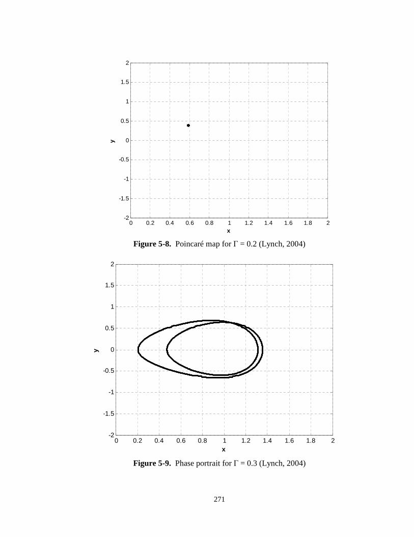
271

Figure 5-8. Poincaré map for Γ = 0.2 (Lynch, 2004)


0 0.2 0.4 0.6 0.8 1 1.2 1.4 1.6 1.8 2-2

-1.5

-1

-0.5

0

0.5

1

1.5

2

x

y

0 0.2 0.4 0.6 0.8 1 1.2 1.4 1.6 1.8 2-2

-1.5

-1

-0.5

0

0.5

1

1.5

2

x

y

272



0 0.2 0.4 0.6 0.8 1 1.2 1.4 1.6 1.8 2-2

-1.5

-1

-0.5

0

0.5

1

1.5

2

x

y

-2 -1.5 -1 -0.5 0 0.5 1 1.5 2-2

-1.5

-1

-0.5

0

0.5

1

1.5

2

x

y

273


5.3.2 Analysis of the Linearly and Nonlinearly Damped Systems using Phase Portraits and Poincaré Maps

The linearly damped system under consideration is

1 ? @ A cos

@ 0,

and the nonlinearly damped system under consideration is

1 ? @ A cos

@ 0.

In order to generate the corresponding Poincaré maps, the system equations had to be

converted to state space form. By letting

3 , 3 , 3 , and 3@ ,

-2 -1.5 -1 -0.5 0 0.5 1 1.5 2-2

-1.5

-1

-0.5

0

0.5

1

1.5

2

x

y

(5.9)

(5.10)

(5.11)

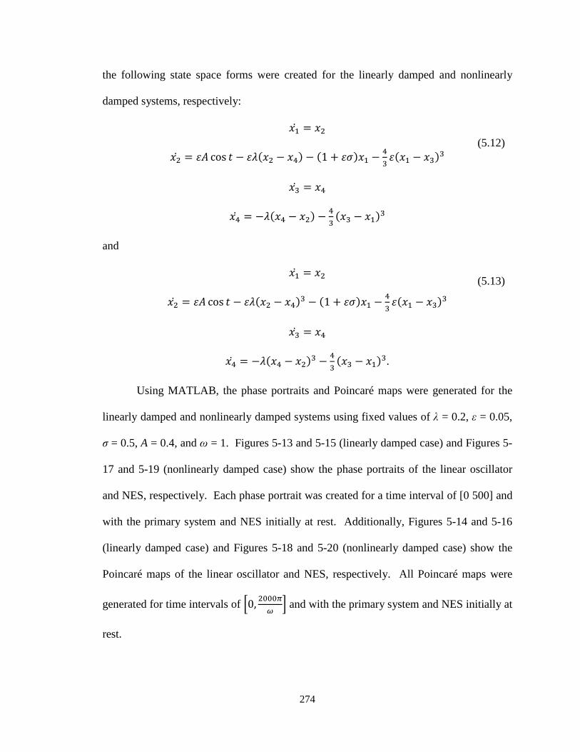
274

the following state space forms were created for the linearly damped and nonlinearly

damped systems, respectively:

3 3

3 A cos 3 3@ 1 ? 3 @ 3 3

3 3@

3@ 3@ 3 @ 3 3

and

3 3

3 A cos 3 3@ 1 ? 3 @ 3 3

3 3@

3@ 3@ 3 @ 3 3 .

Using MATLAB, the phase portraits and Poincaré maps were generated for the

linearly damped and nonlinearly damped systems using fixed values of λ = 0.2, ε = 0.05,

σ = 0.5, A = 0.4, and ω = 1. Figures 5-13 and 5-15 (linearly damped case) and Figures 5-

17 and 5-19 (nonlinearly damped case) show the phase portraits of the linear oscillator

and NES, respectively. Each phase portrait was created for a time interval of [0 500] and

with the primary system and NES initially at rest. Additionally, Figures 5-14 and 5-16

(linearly damped case) and Figures 5-18 and 5-20 (nonlinearly damped case) show the

Poincaré maps of the linear oscillator and NES, respectively. All Poincaré maps were

generated for time intervals of 0, 444¬÷ and with the primary system and NES initially at

rest.

(5.12)

(5.13)

275

Figure 5-13. Phase portrait for the primary system in the case of linear damping

Figure 5-14. Poincaré map for the primary system in the case of linear damping

-0.5 -0.4 -0.3 -0.2 -0.1 0 0.1 0.2 0.3 0.4 0.5-0.5

-0.4

-0.3

-0.2

-0.1

0

0.1

0.2

0.3

0.4

0.5

y1

y 1-do

t

-0.8 -0.6 -0.4 -0.2 0 0.2 0.4 0.6 0.8 1-0.4

-0.2

0

0.2

0.4

0.6

0.8

1

y1

y 1-do

t

276

Figure 5-15. Phase portrait for the NES in the case of linear damping

Figure 5-16. Poincaré map for the NES in the case of linear damping

-1.5 -1 -0.5 0 0.5 1 1.5-1.5

-1

-0.5

0

0.5

1

1.5

y2

y 2-do

t

-2.5 -2 -1.5 -1 -0.5 0 0.5 1 1.5 2 2.5-1.5

-1

-0.5

0

0.5

1

1.5

2

y2

y 2-do

t

277

Figure 5-17. Phase portrait for the primary system in the case of nonlinear damping

Figure 5-18. Poincaré map for the primary system in the case of nonlinear damping

-0.5 -0.4 -0.3 -0.2 -0.1 0 0.1 0.2 0.3 0.4 0.5-0.5

-0.4

-0.3

-0.2

-0.1

0

0.1

0.2

0.3

0.4

0.5

y1

y 1-do

t

-0.8 -0.6 -0.4 -0.2 0 0.2 0.4 0.6 0.8 1-0.4

-0.2

0

0.2

0.4

0.6

0.8

1

y1

y 1-do

t

278

Figure 5-19. Phase portrait for the NES in the case of nonlinear damping

Figure 5-20. Poincaré map for the NES in the case of nonlinear damping

-1.5 -1 -0.5 0 0.5 1 1.5-1.5

-1

-0.5

0

0.5

1

1.5

y2

y 2-do

t

-2.5 -2 -1.5 -1 -0.5 0 0.5 1 1.5 2 2.5-1.5

-1

-0.5

0

0.5

1

1.5

2

y2

y 2-do

t

279

5.3.3 Discussion of Phase Portraits and Poincaré Maps of the Linearly and Nonlinearly Damped Systems

As seen from the Poincaré maps, the information in the phase portraits is greatly

simplified. In the linearly damped case, the orbits in the state space have been reduced to

a “figure-8” shape on the Poincaré map. Similarly, the orbits from the state space of the

linearly damped NES are represented in a simplified shape when sampled in increments

of the period of oscillation as shown on the Poincaré map.

In the case of nonlinear damping, the phase portraits of the linear oscillator show

more orbits close to the origin than in the linearly damped case. The conclusion to be

drawn from these closely spaced orbits is that the displacements and velocities of the

nonlinearly damped system are less than those for the linearly damped system for the

considered parameters in the case presently studied (harmonic forcing near resonance).

Although the phase portrait of the linearly damped NES shows orbits that appear to be

closely spaced near the origin, the orbits of the nonlinearly damped NES are also closely

spaced, but located farther from the origin, indicating that energy pumping is taking place

from the primary system to the nonlinearly damped NES. In addition, the Poincaré maps

corresponding to the linear oscillator and NES in the nonlinearly damped case show

points more tightly packed than those for the linearly damped system, further reinforcing

the previous claim. Note that the structure of the phase portraits and Poincaré maps

remains the same in both linearly and nonlinearly damped systems, but the local density

of orbits (phase portraits) and points (Poincaré maps) varies between the two cases.

280

5.4 Conclusions

This chapter has presented the time-dependent performance of the linearly and

nonlinearly damped systems. First, the time response of the systems to impulse loading

was investigated. From these results, it was evident that the nonlinearly damped NES is

more effective than the linearly damped counterpart only if the magnitude of the impulse

is sufficiently high. Consequently, if the magnitude of impulse if relatively low, the

linearly damped system has a faster reduction in displacement.

The second part of this chapter focused on comparing the phase portraits and

Poincaré maps between the two systems. In the case of harmonic forcing near resonance

( 1 > 1 ? 1⁄ for small ε), the chosen parameters result in the nonlinearly

damped system having lower displacements and velocities than the linearly damped

system. Under these conditions, the nonlinearly damped NES outperforms the linearly

damped NES in regards to vibration attenuation.

281

5.A Appendix

5.A.1 MATLAB Code for Time Response Simulations

%Comparison of system with linear damping and syste m with nonlinear damping %when subjecting to varying impulsive loads close all clear all sigma = 0.5; e = 0.05; lambda = 0.2; m1 = 1; m2 = e ; for A = [5e2 1e3 5e3 1e4 5e4] %Amplitude of impulsive force k = 1; %iteration constant T = 0.01; %time step t_end = 1000; %end of time interval y1 = 0; y2 = 0; y1_NL = 0; y2_NL = 0; t_vec = zeros(1,t_end/T + 1); Y1 = t_vec; Y2 = t_vec; Y1_NL = t_vec; Y2_NL = t_vec; E1 = t_vec; E1_NL = t_vec; E2 = t_vec; E2_NL = t_vec; Y1(1) = y1; Y2(1) = y2; Y1_NL(1) = y1; Y2_NL(1) = y2; z1 = 0; z2 = 0; z3 = 0; z4 = 0; z1_NL = 0; z2_NL = 0; z3_NL = 0; z4_NL = 0; %Runge Kutta 4 %From Fundamentals of Vibrations by Leonard Meirovi tch, p. 677-679: for t = T:T:t_end k = k+1; t_vec(k) = t; %Condition for impulsive force: if k == 2 F=A; else F=0; end %Linear Damping: f11 = z2; f12 = e*F - e*lambda*(z2-z4) - (1+e*sigma)* z1 - ... (4/3)*e*(z1-z3)^3; f13 = z4; f14 = -lambda*(z4-z2) - (4/3)*(z3-z1)^3; g11 = T*f11; g12 = T*f12; g13 = T*f13; g14 = T*f14;

282

f21 = z2 + 1/2*g12; f22 = e*F - e*lambda*((z2+1/2*g12)-(z4+1/2* g14)) - ... (1+e*sigma)*(z1+1/2*g11) - (4/3)*e*((z1 +1/2*g11) - ... (z3+1/2*g13))^3; f23 = z4 + 1/2*g14; f24 = -lambda*((z4+1/2*g14)-(z2+1/2*g12)) - ... (4/3)*((z3+1/2*g13)-(z1+1/2*g11))^3; g21 = T*f21; g22 = T*f22; g23 = T*f23; g24 = T*f24; f31 = z2 + 1/2*g22; f32 = e*F - e*lambda*((z2+1/2*g22)-(z4+1/2* g24)) - ... (1+e*sigma)*(z1+1/2*g21) - (4/3)*e*((z1 +1/2*g21) - ... (z3+1/2*g23))^3; f33 = z4 + 1/2*g24; f34 = -lambda*((z4+1/2*g24)-(z2+1/2*g22)) - ... (4/3)*((z3+1/2*g23) - (z1+1/2*g21))^3; g31 = T*f31; g32 = T*f32; g33 = T*f33; g34 = T*f34; f41 = z2 + g32; f42 = e*F - e*lambda*((z2+g32)-(z4+g34)) - ... (1+e*sigma)*(z1+g31) - (4/3)*e*((z1+g31 )-(z3+g33))^3; f43 = z4 + g34; f44 = -lambda*((z4+g34)-(z2+g32)) - (4/3)*( (z3+g33) - ... (z1+g31))^3; g41 = T*f41; g42 = T*f42; g43 = T*f43; g44 = T*f44; z1 = z1 + 1/6*(g11 + 2*g21 + 2*g31 + g41); z2 = z2 + 1/6*(g12 + 2*g22 + 2*g32 + g42); z3 = z3 + 1/6*(g13 + 2*g23 + 2*g33 + g43); z4 = z4 + 1/6*(g14 + 2*g24 + 2*g34 + g44); y1 = z1; y2 = z3; Y1(k) = y1; Y2(k) = y2; %Energy of mass 1 (primary system): E1(k) = 1/2*m1*z2^2 + 1/2*(1 + e*sigma)*y1^ 2 + 1/3*e*(y1 - y2)^4; %Energy of mass 2 (NES): E2(k) = 1/2*m2*z4^2 + 1/3*e*(y2 - y1)^4; %************************************************** *************** %Nonlinear Damping: f11_NL = z2_NL;

283

f12_NL = e*F - e*lambda*(z2_NL-z4_NL)^3 - ( 1+e*sigma)*z1_NL - ... (4/3)*e*(z1_NL-z3_NL)^3; f13_NL = z4_NL; f14_NL = -lambda*(z4_NL-z2_NL)^3 - (4/3)*(z 3_NL-z1_NL)^3; g11_NL = T*f11_NL; g12_NL = T*f12_NL; g13_N L = T*f13_NL; g14_NL = T*f14_NL; f21_NL = z2_NL + 1/2*g12_NL; f22_NL = e*F - e*lambda*((z2_NL+1/2*g12_NL) - ... (z4_NL+1/2*g14_NL))^3 - (1+e*sigma)*(z1 _NL+1/2*g11_NL) - ... (4/3)*e*((z1_NL+1/2*g11_NL) - (z3_NL+1/ 2*g13_NL))^3; f23_NL = z4_NL + 1/2*g14_NL; f24_NL = -lambda*((z4_NL+1/2*g14_NL) - (z2_ NL+1/2*g12_NL))^3 - ... (4/3)*((z3_NL+1/2*g13_NL)-(z1_NL+1/2*g1 1_NL))^3; g21_NL = T*f21_NL; g22_NL = T*f22_NL; g23_N L = T*f23_NL; g24_NL = T*f24_NL; f31_NL = z2_NL + 1/2*g22_NL; f32_NL = e*F - e*lambda*((z2_NL+1/2*g22_NL) - ... (z4_NL+1/2*g24_NL))^3 - (1+e*sigma)*(z1 _NL+1/2*g21_NL) - ... (4/3)*e*((z1_NL+1/2*g21_NL) - (z3_NL+1/ 2*g23_NL))^3; f33_NL = z4_NL + 1/2*g24_NL; f34_NL = -lambda*((z4_NL+1/2*g24_NL)-(z2_NL +1/2*g22_NL))^3 - ... (4/3)*((z3_NL+1/2*g23_NL) - (z1_NL+1/2* g21_NL))^3; g31_NL = T*f31_NL; g32_NL = T*f32_NL; g33_N L = T*f33_NL; g34_NL = T*f34_NL; f41_NL = z2_NL + g32_NL; f42_NL = e*F - e*lambda*((z2_NL+g32_NL)-(z4 _NL+g34_NL))^3 - ... (1+e*sigma)*(z1_NL+g31_NL) - (4/3)*e*(( z1_NL+g31_NL) - ... (z3_NL+g33_NL))^3; f43_NL = z4_NL + g34_NL; f44_NL = -lambda*((z4_NL+g34_NL)-(z2_NL+g32 _NL))^3 - ... (4/3)*((z3_NL+g33_NL) - (z1_NL+g31_NL)) ^3; g41_NL = T*f41_NL; g42_NL = T*f42_NL; g43_N L = T*f43_NL; g44_NL = T*f44_NL; z1_NL = z1_NL + 1/6*(g11_NL + 2*g21_NL + 2* g31_NL + g41_NL); z2_NL = z2_NL + 1/6*(g12_NL + 2*g22_NL + 2* g32_NL + g42_NL); z3_NL = z3_NL + 1/6*(g13_NL + 2*g23_NL + 2* g33_NL + g43_NL); z4_NL = z4_NL + 1/6*(g14_NL + 2*g24_NL + 2* g34_NL + g44_NL);

284

y1_NL = z1_NL; y2_NL = z3_NL; Y1_NL(k) = y1_NL; Y2_NL(k) = y2_NL; %Energy of mass 1 (primary system): E1_NL(k) = 1/2*m1*z2_NL^2 + 1/2*(1 + e*sigm a)*y1_NL^2 + ... 1/3*e*(y1_NL - y2_NL)^4; %Energy of mass 2 (NES): E2_NL(k) = 1/2*m2*z4_NL^2 + 1/3*e*(y2_NL - y1_NL)^4; end if A == 1e3 lim_x_min = 0; lim_x_max = 80; lim_y = 1; elseif A == 5e3 lim_x_min = 100; lim_x_max = 300; lim_y = 1 ; elseif A == 1e4 lim_x_min = 300; lim_x_max = 500; lim_y = 1 ; elseif A == 5e4 lim_x_min = 300; lim_x_max = 500; lim_y = 1 ; else lim_x_min = 100; lim_x_max = 200; lim_y = 1 ; end figure( 'Units' , 'inches' , 'OuterPosition' , [2 .3 7 10.7]) subplot(4,1,1, 'Units' , 'inches' , 'OuterPosition' , ... [-.3, 7.5, 7.7, 2.3]); plot(t_vec,Y1, '--k' , 'LineWidth' , 2) axis([lim_x_min lim_x_max -lim_y lim_y]) axis 'auto y' hold on; grid on; plot(t_vec,Y1_NL, '-k' , 'LineWidth' , 2) title([ '\bf\itA = ' , num2str(A, '%.0e' )]) ylabel( '\bfDisp. of Main System, \ity_1' ) subplot(4,1,2, 'Units' , 'inches' , 'OuterPosition' , ... [-.3, 5, 7.7, 2.3]); plot(t_vec,Y2, '--k' , 'LineWidth' , 2) axis([lim_x_min lim_x_max -lim_y lim_y]) axis 'auto y' hold on; grid on; plot(t_vec,Y2_NL, '-k' , 'LineWidth' , 2) ylabel( '\bfDisp. of NES, \ity_2' ) subplot(4,1,3, 'Units' , 'inches' , 'OuterPosition' , ... [-.3, 2.5, 7.7, 2.3]); plot(t_vec,E1, '--k' , 'LineWidth' , 2) axis([lim_x_min lim_x_max -lim_y lim_y]) axis 'auto y' hold on; grid on; plot(t_vec,E1_NL, '-k' , 'LineWidth' , 2) ylabel( '\bfEnergy of Main System, \itE_1' ) subplot(4,1,4, 'Units' , 'inches' , 'OuterPosition' , ...

285

[-.3, 0, 7.7, 2.3]); plot(t_vec,E2, '--k' , 'LineWidth' , 2) axis([lim_x_min lim_x_max -lim_y lim_y]) axis 'auto y' hold on; grid on; plot(t_vec,E2_NL, '-k' , 'LineWidth' , 2) xlabel( '\bfTime, \itt' ) ylabel( '\bfEnergy of NES, \itE_2' ) end

5.A.2 MATLAB Code for Phase Portrait and Poincaré Examples

%Examples for Chapter 5 %Based on examples given by Lynch (2004) close all clear all k = 0.3; w = 1.25; for gamma = [0.2 0.3] x = 1; y = 0; theta = 0; ind = 0; ind2 = 0; p = 0; n = 2; dt = 0.001; t_end = 400; t_steady = t_end - 100 ; t_period = t_steady; for t = dt:dt:t_end ind = ind + 1; x_dot = y; y_dot = x - k*y - x^3 + gamma*cos(theta); theta_dot = w; x = x + x_dot*dt; y = y + y_dot*dt; theta = theta + theta_dot*dt; if abs(theta - n*pi) < 0.001 n = n + 2; else end if t > t_steady ind2 = ind2 + 1; X(ind2) = x; Y(ind2) = y; if abs(theta - n*pi) < 0.01 p = p + 1; X_p(p) = X(ind2); Y_p(p) = Y(ind2); else

286

end else end end %Plot State-Space: figure plot(X,Y, '-k' , 'LineWidth' ,2) axis([0 2 -2 2]); grid on; xlabel( '\bfx' ); ylabel( '\bfy' ); %Plot Poincare Map: figure plot(X_p,Y_p, '.k' ) axis([0 2 -2 2]); grid on; xlabel( '\bfx' ); ylabel( '\bfy' ); end clear all %The following code is based on those given by Lync h (2004): state_space = inline( '[x(2);x(1)-0.3*x(2)-(x(1))^3 + 0.5*cos(1.25*t)]' , 't' , 'x' ); options = odeset( 'RelTol' ,1e-4, 'AbsTol' ,1e-4); [t,x_ss] = ode45(state_space,[0 200],[1,0], options ); [t,x_p] = ode45(state_space,0:2*pi/1.25:4000*pi/1.2 5,[1,0]); %Plot State-Space: figure plot(x_ss(:,1),x_ss(:,2), '-k' , 'LineWidth' ,2) axis([-2 2 -2 2]); grid on; xlabel( '\bfx' ); ylabel( '\bfy' ); %Plot Poincare Map: figure plot(x_p(:,1),x_p(:,2), '.k' ) axis([-2 2 -2 2]); grid on; xlabel( '\bfx' ); ylabel( '\bfy' );

5.A.3 MATLAB Code for Phase Portraits

%Phase portraits for the systems with linear and no nlinear damping %Based off of code used by Lynch (2004) close all clear all %lambda = 0.2; sigma = 0.5; e = 0.05; A = 0.4;

287

%Linear damping case: w = 1; t_end = 500; state_space = inline( '[x(2); .05*0.4*cos(t) - .05*0.2*(x(2)-x(4)) - (1+.05*0.5)*x(1) - 4/3*.05*(x(1)-x(3))^3; x(4); -0. 2*(x(4)-x(2)) - 4/3*(x(3)-x(1))^3]' , 't' , 'x' ); [t, x_vec] = ode45(state_space,[0 t_end],[0,0,0,0]) ; figure plot(x_vec(:,1),x_vec(:,2), '-k' ) xlabel( '\bfy_1' ); ylabel( '\bfy_1-dot' ) figure plot(x_vec(:,3),x_vec(:,4), '-k' ) xlabel( '\bfy_2' ); ylabel( '\bfy_2-dot' ) clear all %Nonlinear damping case: w = 1; t_end = 500; state_space = inline( '[x(2); .05*0.4*cos(t) - .05*0.2*(x(2)-x(4))^3 - (1+.05*0.5)*x(1) - 4/3*.05*(x(1)-x(3))^3; x(4); -0. 2*(x(4)-x(2))^3 - 4/3*(x(3)-x(1))^3]' , 't' , 'x' ); [t, x_vec] = ode45(state_space,[0 t_end],[0,0,0,0]) ; figure plot(x_vec(:,1),x_vec(:,2), '-k' ) xlabel( '\bfy_1' ); ylabel( '\bfy_1-dot' ) figure plot(x_vec(:,3),x_vec(:,4), '-k' ) xlabel( '\bfy_2' ); ylabel( '\bfy_2-dot' )

5.A.4 MATLAB Code for Poincaré Maps

%Poincare maps for the systems with linear and nonl inear damping %Based off of code used by Lynch (2004) close all clear all %lambda = 0.2; sigma = 0.5; e = 0.05; A = 0.4; %Linear damping case: w = 1; dt = 2*pi/w; t_end = 2000*pi/w;

288

state_space = inline( '[x(2); .05*0.4*cos(t) - .05*0.2*(x(2)-x(4)) - (1+.05*0.5)*x(1) - 4/3*.05*(x(1)-x(3))^3; x(4); -0. 2*(x(4)-x(2)) - 4/3*(x(3)-x(1))^3]' , 't' , 'x' ); [t, x_vec] = ode45(state_space,0:dt:t_end,[1,0,0,0] ); figure plot(x_vec(:,1),x_vec(:,2), '.k' ) xlabel( '\bfy_1' ); ylabel( '\bfy_1-dot' ) axis([-0.8 1 -0.4 1]) figure plot(x_vec(:,3),x_vec(:,4), '.k' ) xlabel( '\bfy_2' ); ylabel( '\bfy_2-dot' ) axis([-2.5 2.5 -1.5 2]) clear all %Nonlinear damping case: w = 1; dt = 2*pi/w; t_end = 2000*pi/w; state_space = inline( '[x(2); .05*0.4*cos(t) - .05*0.2*(x(2)-x(4))^3 - (1+.05*0.5)*x(1) - 4/3*.05*(x(1)-x(3))^3; x(4); -0. 2*(x(4)-x(2))^3 - 4/3*(x(3)-x(1))^3]' , 't' , 'x' ); [t, x_vec] = ode45(state_space,0:dt:t_end,[1,0,0,0] ); figure plot(x_vec(:,1),x_vec(:,2), '.k' ) xlabel( '\bfy_1' ); ylabel( '\bfy_1-dot' ) axis([-0.8 1 -0.4 1]) figure plot(x_vec(:,3),x_vec(:,4), '.k' ) xlabel( '\bfy_2' ); ylabel( '\bfy_2-dot' ) axis([-2.5 2.5 -1.5 2])

289

6.0 Conclusions and Recommendations

6.1 Summary of Work Presented

This thesis has presented analytical and numerical comparisons between single-degree of

freedom linear systems with linearly and nonlinearly damped nonlinear energy sink

(NES) attachments. Chapter 1 provided an introduction to NES and a background of

previous related work. Concepts such as targeted energy transfer, nonlinear normal

modes (NNMs), and resonance capture were discussed to provide the reader prerequisite

information for understanding how NES achieve energy pumping. Comparisons between

classical linear vibration absorbers and NES were presented in order to instill motivation

for studying NES. Finally, experimental methods used in the study of NES were

illustrated.

Chapter 2 focused on the differences between various single-degree of freedom

systems. A linear system, a NES system, and a nonlinear system with nonlinear damping

were compared in terms of time response, system energy as a function of time, and

energy decay as a function of time. In each performance comparison, the nonlinear

system with nonlinear damping exhibited the most desirable characteristics in regards to

vibration attenuation. Clearly, the nonlinear damping allowed the nonlinear system to

dissipate energy faster than its linearly damped counterparts, thus providing a more rapid

reduction in displacement.

Saddle-node and Hopf bifurcations of the single-degree of freedom linear systems

with linearly and nonlinearly damped NES were presented in Chapter 3 in order to study

the periodic behavior of the two systems. The saddle-node bifurcation diagrams showed

290

boundaries between one and three real periodic solutions. Boundaries separating stable

and unstable regions were shown by the Hopf bifurcation diagrams. Qualitative

differences between the two systems were discussed by comparing the bifurcation

diagrams of each system for the same sets of parameters.

Chapter 4 deviates from the analysis of periodic solutions by comparing the

Strongly Modulated Response (SMR) between the linearly and nonlinearly damped

systems. First, the projection of the slow invariant manifold (SIM) onto a 2-D plane of

system parameters was presented to show the locations for the jumps of the system

response between stable branches. Phase portraits were presented for the stable branches

of the SIM in order to show the manner in which the system response can jump between

these branches. For a concise illustration of the trajectories that leave the lower fold line

and eventually return, 1-D maps of the phase angles were constructed for varying the

system parameter σ. A range of σ that permitted the return trajectories was determined,

thus providing the conditions for the existence of the SMR. Due to the correlation

between σ and the forcing frequency, frequency ranges were determined that allow for

the SMR to occur.

In Chapter 5, time response comparisons were made between the linearly and

nonlinearly damped systems. Plots of displacement and energy versus time were

presented for the systems with varying amplitudes of impulse loading. From these

numerical simulations, it was determined that the displacement and energy of the linear

oscillator decay faster in the linearly damped system than the nonlinearly damped system

for low impulse amplitudes. However, if the impulse amplitude is increased beyond a

certain level, the performance of the nonlinearly damped system becomes more desirable

291

in terms of vibration attenuation than the linearly damped system. Performance

comparisons of the periodically forced system were continued with the use of phase

portraits and Poincaré maps. Comparisons between these plots reveal that the nonlinearly

damped system in general has lower displacements and velocities than the linearly

damped system for the chosen system parameters.

One should keep in mind that this thesis has investigated the performance of the

single-degree of freedom systems with linearly and nonlinearly damped NES for only

specific cases. Periodic forcing near resonance was studied in Chapters 3 through 5, and

the SMR discussed in Chapter 4 was only possible due to the 1:1 resonance with the

linear oscillator. Additionally, only specific parameters were chosen to illustrate the

system behavior for these cases.

6.2 Suggested Future Work

In order to expand on the work presented in this thesis, the obvious suggestion is to

repeat the work using different system parameters. Using the methods presented, this

variation should be straightforward to implement. Additionally, the systems could be

investigated to determine their behavior when subjected to periodic forcing away from

1:1 resonance, although the SMR will not exist in this case.

Prior to attempting to apply the work shown in this thesis to practical engineering

applications, experiments should be run to confirm these conclusions. Even after the

analytical and numerical results have been correlated to experiments, one must determine

a method of physically implementing the system parameters in the design. Piecewise

nonlinear damping can be achieved in practice via the variable orifice discussed by

Starosvetsky and Gendelman (2009), but this nonlinear damping differs from the

292

damping discussed in the work of this thesis. Nonlinear stiffness has been achieved in

experiments by using a grounded wire as shown in Section 1.4 of Chapter 1 of this thesis,

but the designer of an engineering application involving NES must determine if this

method is suitable for a particular situation. This thesis presents only preliminary work

on nonlinearly damped NES, and much work still remains before practical applications

can be implemented.

6.3 Practical Applications of Nonlinear Energy Sinks

Before deciding to use nonlinear energy sinks in a design, it is important to consider the

application. In some cases, a linear vibration absorber may be desired due to its

simplicity of design and likely cost savings. For example, if vibration at a single resonant

frequency is the only concern, a tuned linear absorber is a logical option. However, if the

application demands attenuation at multiple frequencies and/or a more reliable design, a

nonlinear energy sink is advantageous. Furthermore, the use of linear versus nonlinear

damping in the NES design should be given consideration as well. If the external forces

on the system are very high, a NES with nonlinear damping would likely result in more

efficient energy reduction in the primary system than a NES with linear damping.

293

7.0 References Gendelman, O.V. (2001). Transition of energy to a nonlinear localized mode in a highly asymmetric system of two oscillators, Nonl. Dyn. 25, 237-253. Gendelman, O.V., and Y. Starosvetsky (2007). Quasiperiodic response regimes of linear oscillator coupled to nonlinear energy sink under periodic forcing, Journal of Applied Mechanics 74, 325-331. Gendelman, O.V., L.I. Manevitch, A.F. Vakakis, and R. M’Closkey (2001). Energy Pumping in Nonlinear Mechanical Oscillators: Part I – Dynamics of the Underlying Hamiltonian Systems, Journal of Applied Mechanics 68, 34-41. Gendelman, O.V., Y. Starosvetsky, and M. Feldman (2008). Attractors of harmonically forced linear oscillator with attached nonlinear energy sink I: description of response regimes, Nonlinear Dynamics 51, 31-46. Lee, Y.S., A.F. Vakakis, L.A. Bergman, D.M. McFarland, G. Kerschen, F. Nucera, S. Tsakirtzis, and P.N. Panagopoulos (2008). Passive non-linear targeted energy transfer and its applications to vibration absorption: a review, IMechE 222, 77-134. Lynch, S. (2004). Dynamical Systems with Applications Using MATLAB, Birkhäuser, Boston. Meirovitch, L. (2001). Fundamentals of Vibrations, McGraw-Hill, New York. Nayfeh, A. H. and Balachandran, B. (1995). Applied Nonlinear Dynamics: Analytical, Computational, and Experimental Methods, Wiley, New York. Nayfeh, A. H. and Mook, D. T. (1995). Nonlinear Oscillations, Wiley, New York. Rand, R. (2005). Lecture Notes on Nonlinear Vibrations, Richard H. Rand. Sanders, J., and F. Verhulst (1985). Averaging Methods in Nonlinear Dynamical Systems, Springer-Verlag, New York. Starosvetsky, Y., and O.V. Gendelman (2008). Response regimes of linear oscillator coupled to nonlinear energy sink with harmonic forcing and frequency detuning, Journal of Sound and Vibration 315, 746-765. Starosvetsky, Y., and O.V. Gendelman (2008). Strongly modulated response in forced 2DOF oscillatory system with essential mass and potential asymmetry, Physica D 237, 1719-1733. Starosvetsky, Y., and O.V. Gendelman (2009). Vibration absorption in systems with a nonlinear energy sink: Nonlinear damping, Journal of Sound and Vibration 324, 916-939. Stewart, J. (1999). Calculus Early Transcendentals, Brooks/Cole Publishing Company, Pacific Grove. Vakakis, A.F. (2001). Inducing Passive Nonlinear Energy Sinks in Vibrating Systems, Journal of Vibration and Acoustics/Transactions of the ASME 123, 324-332.

294

Vakakis, A.F., L.I. Manevitch, O. Gendelman, and L. Bergman (2003). Dynamics of linear discrete systems connected to local, essentially non-linear attachments, Journal of Sound and Vibration 264, 559-577. Vakakis, A.F., O.V. Gendelman, L.A. Bergman, D.M. McFarland, G. Kerschen, and Y.S. Lee (2008). Nonlinear Targeted Energy Transfer in Mechanical and Structural Systems I, Springer, New York. Zwillinger, D. (2003). CRC Standard Mathematical Tables and Formulae, Chapman & Hall/CRC Press LLC, Boca Raton.

Documents

ENERGY SINKS WITH NONLINEAR STIFFNESS AND NONLINEAR DAMPING