NASA/CR-2000-210557

ICASE Report No. 2000-43

An Energy Decaying Scheme for Nonlinear Dynamics

of Shells

Carlo L. Bottasso

Politecnico di Milano, Milano, Italy

Olivier A. Bauchau and Jou-Young Choi

Georgia Institute of Technology, A tlanta, Georgia

November 2000

https://ntrs.nasa.gov/search.jsp?R=20000121222 2018-05-22T23:15:57+00:00Z

The NASA STI Program Office... in Profile

Since its founding, NASA has been dedicated

to the advancement of aeronautics and spacescience. The NASA Scientific and Technical

Information (STI) Program Office plays a key

part in helping NASA maintain this

important role.

The NASA STI Program Office is operated by

Langley Research Center, the lead center forNASA's scientific and technical information.

The NASA STI Program Office provides

access to the NASA STI Database, the

largest collection of aeronautical and space

science STI in the world. The Program Office

is also NASA's institutional mechanism for

disseminating the results of its research and

development activities. These results are

published by NASA in the NASA STI Report

Series, which includes the following report

types:

TECHNICAL PUBLICATION. Reports of

completed research or a major significant

phase of research that present the results

of NASA programs and include extensive

data or theoretical analysis. Includes

compilations of significant scientific andtechnical data and information deemed

to be of continuing reference value. NASA's

counterpart of peer-reviewed formal

professional papers, but having less

stringent limitations on manuscript

length and extent of graphic

presentations.

TECHNICAL MEMORANDUM.

Scientific and technical findings that are

preliminary or of specialized interest,

e.g., quick release reports, working

papers, and bibliographies that containminimal annotation. Does not contain

extensive analysis.

CONTRACTOR REPORT. Scientific and

technical findings by NASA-sponsored

contractors and grantees.

CONFERENCE PUBLICATIONS.

Collected papers from scientific and

technical conferences, symposia,

seminars, or other meetings sponsored or

cosponsored by NASA.

SPECIAL PUBLICATION. Scientific,

technical, or historical information from

NASA programs, projects, and missions,

often concerned with subjects having

substantial public interest.

TECHNICAL TRANSLATION. English-

language translations of foreign scientific

and technical material pertinent to

NASA's mission.

Specialized services that complement the

STI Program Office's diverse offerings include

creating custom thesauri, building customized

data bases, organizing and publishing

research results.., even providing videos.

For more information about the NASA STI

Program Office, see the following:

• Access the NASA STI Program Home

Page at http://www.sti.nasa.gov

• Email your question via the Internet to

help@sti.nasa.gov

• Fax your question to the NASA STI

Help Desk at (301) 621-0134

• Telephone the NASA STI Help Desk at

(301) 621-0390

Write to:

NASA STI Help Desk

NASA Center for AeroSpace Information7121 Standard Drive

Hanover, MD 2 !076-1320

NASA/CR-2000-210557

ICASE Report No. 2000-43

An Energy Decaying Scheme for Nonlinear Dynamicsof Shells

Carlo L. Bottasso

Politecnico di Milano, Milano, Italy

Olivier A. Bauchau and Jou- Young Choi

Georgia Institute of Technology, Atlanta, Georgia

ICASE

NASA Langley Research Center

Hampton, Virginia

Operated by Universities Space Research Association

National Aeronautics and

Space Administration

Langley Research Center

Hampton, Virginia 23681-2199

Prepared for Langley Research Centerunder Contract NASI-97046

November 2000

Available from the following:

NASA Center for AeroSpace Information (CASI)7121 Standard Drive

Hanover, MD 21076-1320

(301) 621-0390

National Technical Information Service (NTIS)

5285 Port Royal Road

Springfield, VA 22161-2171

(703) 487-4650

AN ENERGY DECAYING SCHEME FOR NONLINEAR DYNAMICS OF SHELLS

CARI,O 1,. BOTTASSO*, OIAVIER A. BAUCHAtI?, AND JOU-YOUNG CHOI_

Abstract. A novel integration scheme for nonlinear dynamics of geometrically exact shells is developed

based on the inextensible director assumption. The new algorithm is designed so as to imply the strict decay

of the system total mechanical energy at each time step, and consequently unconditional stability is achieved

in the nonlinear regime. Furthermore, the scheme features tunable high frequency numerical damping and

it is therefore stiffly accurate. The method is tested for a finite element spatial formulation of shells based

on mixed interpolations of strain tensorial components and on a two-parameter representation of director

rotations. The robustness of the scheme is illustrated with the help of numerical examples.

Key words, geometrically exact shell, time integration, energy decaying scheme

Subject classification. Applied and Numerical Mathematics

1. Introduction. The formulation of integration algorithms for nonlinear dynamics of geometrically

exact shells is the focus of this work. The partial differential equations governing this class of problems are

known to present a rich mathematical structure. In particular, the resulting models are Hamiltonian systems

characterized by a symplectic nature and associated with conservation laws that stem from symmetries of

the Hamiltonian. The linear and angular momentum as well as the total mechanical energy are conserved

for free motions of such systems.

The understanding of the geometric characteristics of the governing equations has been historically

confined to the fields of analytical mechanics and pure mathematics. Surprisingly, this knowledge has been

seldom used for the development of numerical methods. Indeed, the study of new integration algorithms has

been traditionally preoccupied with the development of methods applicable to vast (:lasses of problems, for

example the class of differential/algebraic equations, or hyperbolic conservation laws. Consequently: classical

methods rarely preserve the underlying structure of the problem being solved, and hence, such structure is

lost in the numerical solution.

This approach also limits the possible theoretical analyses of the schemes, which are, more often than

not, confined to linear or model cases. For instance, it is customary to characterize integration schemes

for structural dynamics by studying their behavior when applied to a linear oscillator. This approach is

clearly not adequate when dealing with highly nonlinear problems such as the dynamics of geometrically

exact shells.

A new approach to the design of integration algorithms attempts to bridge the divide between theoretical

and numerical mechanics. Under this new paradigm, numerical schemes are "backward-engineered" to

preserve some important qualitative features of the governing equations. Fittingly, this approach is now

called geometric integration in the mathematical community [18]. Attempts at designing "geometry-aware"

algorithms for structural dynamics problems can be traced back to the work of Simo and co-workers who

"Dipartimento di lngegneria Aerospaziale, Politecnico di Milano, Via La Masa 34, 20158 Milano, Italy (email address:

Carlo.Botta.sso_polimi.it). This research was supported by the National Aeronautics and Space Administration under NASAContract No. NAS1-97046 while the first author wa_sin residence at ICASE, NASA Langley Research Center, Hampton, VA23681-2199.

?Georgia lnslitute of Technology, School of Aerospace Engineering, Atlanta, GA, USA (email address:

Olivier Bauchau_aerospace.gat ech .edu).tGeorgia Institute of Technology, School of Aerospace Engineering, Atlanta, GA, USA.

analyzedtheproblemsof rigidbodydynamics[26],nonlinearelasto-dynamics[23],geometricallyexact

shells [241, and geometrically exact beams [25]. In all cases, the idea was to design algorithms that ensure

the discrete preservation of the total mechanical energy and of the linear and angular momenta of tile system.

When integrating linear and nonlinear finite element models, the implications of tile discrete equations

stiffness must be careflllly considered. Indeed, high frequencies are an artifact of the spatial discretization

process and do not reflect the high frequencies of the original infinite dimensional problem. The need for

high frequency numerical dissipation has been recognized in the past for linear problems [20]. When dealing

with complex nonlinear systems, numerical dissipation becomes indispensable. Indeed, nonlinearities provide

a mechanism for transferring energy from low to high frequency modes. Consequently, numerical solutions

feature violent oscillations of a purely numerical origin that will eventually play havoc with the convergence

characteristics of the nonlinear equation solver.

Among the various geometric characteristics of shell equations, energy preservation appears to be the

most important for the development of robust time integration schemes. In fact, strict energy preservation

at the discrete lew_l leads to uncondif.ional stability i'n. the nonlinear regime, whereas the classical approach

based on the analysis of the spectral radius leads to unconditional stability in the linear regime only. An

energy preserving (EP) scheme for geometrically exact shell is developed in this paper. In addition, the

scheme also preserves both linear and angular momenta of the system at the discrete level. Unfortunately,

preservation of energy and high frequency dissipation cannot coexist, unless energy is transferred from high

to low frequency modes, a transfer that has no physical basis. To solve this problem, a family of energy

decaying (ED) schemes that imply a controllable energy decay within each time step is proposed in this work.

In geometric terms, this means that the evolution of the system is not confined to the level set of constant

energy, but is allowed to drift away from it in a monotonic and controllable manner. Since the energy remains

bounded at all times, the scheme is unconditionally stable for nonlinear systems. Furthermore, it can be

shown that the energy dissipation mechanism of the algorithm is the result of the removal of the higher

frequencies from the computed response.

In related papers, various energy preserving and decaying geometric integrators were developed for rigid

bodies and geometrically exact beams [10, 11, 14, 6, 7], and nonlinear elastodynamics [9]. The concepts

were extended to multibody systems featuring nonlinear holonomic constraints [:3, 15, 12, 16, 1:3]; non-

holonomic and unilateral constraints were treated in [5, 4]. The integration of the present shell model in a

general finite element based multibody framework is discussed in [8]. The proposed scheme is independent

of the choice of spatial discretization applied to the governing partial differential equations. In the present

implementation, the finite element method is used, and the mixed interpolation of tensorial components [1,

2, 17] is implemented to avoid the shear locking problem. The orientation of unit shell directors is described

by a special family of two-parameter rotations.

The paper is laid out as follows. The classical equations of motion for geometrically exact shells based

on inextensible unit directors are presented in section 2. Next, an EP scheme is developed in section :3.

Section 4 then presents an ED algorithm with tunable high frequency dissipation that is constructed flom

the EP scheme. Finally, numerical examples are presented in section 5 to demonstrate the efficiency and

robustness of the proposed scheme. A discussion section concludes the paper.

2. Formulation of the Equations of Motion.

2.1. Kinematics of the Shell Problem. Consider a shell of thickness h and reference surface area f_,

as depicted in fig. 2.1. An inertial frame of reference $ consisting of three mutually orthogonal unit vectors

i_, i2, i3 is used. Let _r0 be the position vector of an arbitrary point on the reference surface of the shell, and

Reference

U • E 2configuration_ .... _--_--..

/J_ / Deformed

'_ . /_--¢-2 / configuration

Ti3 //i2

Fie;. 2.1. Configuration of the shell in the reference and deformed configurations.

let. ¢ be the material coordinate along n_, the normal to the reference surface. The position vector _r of an

arbitrary point on the shell in its reference configuration is then

7/ 1 2__((1 4_,( ) = _((, ,(2) + _ _(4 ,(), (2.1)

where 41 and 42 are the material coordinates used to represent the shell reference surface. The coordinates

(_, (2 and ( form a set of curvilinear coordinates that are a natural choice to represent the shell geometry.

The coordinates (_and (2 are assumed to be lines of curvatures of the shell reference surface. The base

vectors are then

•q = "qt' "-q2' "-q3 = r,t, r,2, = (1 - RI R2

where R1 and R2 are the principal radii of curvature, a_. = r-0._,, and the notation (-),_ is used to denote a

derivative with respect to 4 °. It is convenient to introduce a set. of three mutually orthogonal unit vectors

at the shell reference surface (i.e. at ( = O)

al a2e 1 =--; e 2= " e,_ =n, (2.3)

_v_,_' -

where aa,_ - a, • ac_.

Two fundamental assumptions will be made concerning the defi)rmation of the shell, i.e. the material

line initially normal t.o the reference surface of the shell remains a straight, line and suffers no extension.

This is the classical inextensible director model. With these assumptions, the position vector of a material

point, of the shell writes

_(4',4 _,() = _(4',4 _) + _(4',(2) + ( _E3(4, ,4_), (2.4)

whereu(_ 1 ,_2) is the reference surface displacement vector, hi tile deformed configuration, the base vectors

at. the shell reference surface are

= [a_;, g-2, G_31= [/7,G

Introducing the position vector, eq. (2.4), then yields

a=[a', -<' ]

where

_t I IL,2E:[E_, E2,£3]= _,+ -" _e_+- '

, _R,,,

= E + ( H, (2.6)

Note that E___((l, _2) is a unit vector, whereas E 1 and __E2 are not unit vectors, nor are they orthogonal to

E3, as axial and transverse shearing strains develop dm'ing deformation.

2.2. Equations of Motion. The Green-Lagrange strain tensor e is defined as

1e = 7(arc - .or.q). (2.8)

The strain tensor e is defined in the curvilinear coordinate system defined by coordinates _1,(2 and (.

However, it is more convenient to work with the strain tensor e defined in the locally rectangular system

defined by triad e__.l,e_.2,£3, see eqs. (2.3). For shallow shells (i.e. (/R1 << 1 and (/R2 << 1) undergoing large

displacements and rotations but small strains (all strain components are assumed to be small compared to

unity), the strain-displacement relationships can be written as

e = 21[EWE_ S + ( (ET H + HT E + n)] , (2.9)

where

1/B_ 0 0 1n= 0 1//72 0 . (2.10)

0 0 0

It is clear that the strains can be expressed in terms of five parameters: the three components of the

displacement field L_ (through E I and E._) and the two parameters defining the orientation of the unit

director E a. Virtual changes in the strain energy of the structure are given by

<_V= f_ L _f" d(dfl = in L & •r d(drl , (2.11)

where 77I-"is the virtual strain energy density, and r the second Piola-Kirchhoff stress tensor. Introducing

the strains, eq. (2.9), and taking into account the symmetry of the stress tensor then yields

_V : <_E. (E + (U)r + 6H-<E_-. (2.12)

The existence of a strain energy density function 17 is postulated here, hence the constitutive laws are of the

form r = 0f'/0e.

The velocity vector of material point P of the shell is obtained by differentiating the position vector,

eq. (2.4), with respect to time, to find _v= _fi+ (_E3. The kinetic energy of the system is now

I,L 'LLK = /_" d(dfl = 7 p £-L' d(dft, (2.13)

wheref( is thekineticenergy,density.Int.roducingthevelocityvectorthenyMds

1K = _ p (_ + _£a) ('J + (_3)

Hamilton's Principle can now be expressed as

(2.14)

+ (6 _Ea) - (ii + (_a) + fiE. (E + (H)T + gill. (Er] d(dfidt

= 0. (2.15)

Integrating through the thickness of the shell, we get

f" _ {&,. ['h- (Nl,t + N2,2) ] + a___E-[._q!- (t'_L,,, + M2,2)+ N3]} dftdt = 0. (2.16)

In this expression, h = m_ + s*/}Ta, and ._q= s*_u + [*_73 are the linear and angular momentum vectors of

the shell, respectively; the mass coefficients are defined a_s m = fh P d(, s* = .fh P¢ d<, [* = .fh P(_ d¢.

The in-plane forces are .32"_= (EN*_ + H_)/ax/-ff_ , the out-of-plane forces N 3 = EN* 3, and the bending

__ = • * r* d_, and the convectedmoments M_, (EM_)/av/gTg_. The convected forces are N* = [N 1 ,N2,N3] = .fh r

bending moment.s M* = [M_, M;, M_] = .fh r( d(.

The equations of motion of shells could be derived from this principle by expressing the variations a__E3

in terms of two components of virtual rotation.

3. Energy Preserving Scheme. Discrete equations of motkm that imply discrete conservation laws

for the total mechanical energy, linear momentum and angular momentum of the system will now be de-

veloped. Times t, and t.r denote the initial and final times for a time step, respectively, and the subscripts

(')i and (')I indicate quantities at ti and t I, respectively. Furthermore, the subscript (')m is used to denote

mid-point average quantities defined as

1

(')m = _ [(')f + (')i1. (3.1)

The following matrix identity will be used extensively

AyBI - ATB, = (& - A,)rBm + A/,(BI - BJ. (3.2)

Hamilton's Principle, eq. (2.15), is now approximated in time in the the following manner

[a,-a, At JL

+ <H,,)r,, + (HI - Hi)" (E_r,} dg,tf_ = 0. (3.3)+(EI E,) .

The change in strain components from ti to tI is evaluated with the help of identity (3.2) to find

1e s - e, = _ [(E, - Ei)r(Em + (Hm) + (E_ + (H,,,)r(EI - E_)

+(H I - Hi)T<E,,, + (E_(H I - Hi)]. (3.4)

Overonetimestep,thestraincomponentscarlbeapproximatedase(tl) =em + rl(e I - ei)/2, where 17=

2(t, - t,,)/._kt is the non-dimensional time. If the strain energy density fimction V is viewed as a fimclion of

the scalar variable q, the mean vahle theorem then implies the existence of a f/ E [-1, 1] such that

0iT: _ def) = _', + _ _2 = _i + _,-(_: - e,). (3.5)

This relationship defines the average second Piola-Kirchhoff stress tensor, 7-,_= O('/Oelo. Combining this

result with eq. (3.4) then leads to

(e: - e_). (E,, + CHm)_o+ (e: - H_). <e,,_ : (e: e,). _-_,: _? - _, (3.6)

where the symmetry of the stress tensor was taken into account. For linear constitutive laws of the form

_- = C* e, where C* is the stiffness matrix, the average stress tensor simply hecomes T_ = C* era.

The following configuration updates are now defined

u: - _u_ . _e3: - _e3_ _ _3,,_- (3.7)At -- _u,,; At

Introducing eqs. (3.6) and (3.7) into the approximate expression for Hamilton's Principle, eq. (3.3), then

leads to

--

= L _ [(K:- I:,:)+ (g_r- fS)] d_dn = o. (3.8)

Tiffs result clearly implies the conservation of the total mechanical energy of the system within a step.

In summary, the approximate form of Hamilton's Principle given by eq. (3.3) leads to a discrete energy

conservation statement, eq. (3.8), when the configuration updates are chosen according to eqs. (3.7), and the

average stress according to eq. (3.5).

Integrating through the thickness of the shell leads to

[LLZL' + N_m._)]f_, {('-':- _') L ±' (_x,,_,,

+ (/_3/ -- E-E--3i) " [ /_t (/_/I m,'l + ]_--f2rn,'2) + N3rrt dn = 0. (3.9)

In this expression, the in-plane forces are N,_,,, = (E,,N*_<, + H,,M_,)/a_, the out-of-plane forces N3m =

EmN:],,, and the bending moments -_-_m = (EmM*_,_)/ax/5_" The discrete governing equations of motion

for shells are then

]'tf -- ]'t i

_ (N,_,, + N__,.,_)= p; (3.1o)

QT 'q-: - '-q_ •rn {..._ QTI (i_'flm,1 + 1_/2m,2 -- N3rn) = qm' (3.11)

where p are the externally applied loads, and q_ the externally applied moments meamared in the local

system. The finite change in director orientation __E3I - E3, was expressed in terms of the two parameter

incremental rotation vector, see B.

InvarianceofthesystemHamiltonianunderspatialtranslationsandrotationsimpliestheconservationofthelinearandangularmomenta.Althoughdiscretepreservationofmomentais lesscrucial than discrete

preservation of energy, it is interesting to note that eqs. (3.10) and (3.11) also imply the discrete preservation

of this invariant. At first, eqs. (3.10) are projected onto the test fllnctions _(r-0 + urn) and eqs. (3.11) onto

the test. timer.ions ___Eam, where _ is an arbitrary vector. Next,, integration over the shell reference sm'face

yields

[hi 2 h,(N,m,, + N._,.,2)]

9I - .qi+ _E._ " [--_-

Straightforward algebraic manipulations then lead to

W ]} dFt=0. (3.12)

+ _I'qI - _i.qi + _m(El - _/)] aft = o, (3.13)

where the following result was used

_, mN,m + E--'2mN2m + _a,, mM,m + _3,._,,,-AL_,,, + E._mN3,, = 0. (3.14)

Inserting the configuration updates, eqs. (3.7), into eq. (3.13) then yields

/'k_," [(_0 ÷ U'_' ) hs - (?-° ÷ _i) L_/÷ _-E-3f'q/ - -E-E3i-gi ÷ (-_hm_:'n ÷ "--m _-_3m) ] d_=0" (3.15)

It. is easily verified that. -_hmu_"m + -_rnF...___3n, : O. Hence, since 7r is arbitrary, eq. (3.15) implies the discrete

conservation of the total angular momentum, ./n[(_70 + _) h + _ 9__]dft. Finally, projecting eqs. (3.10) onto

the test. fllnctions 7r and eqs. (3.11) ont.() the null test functions gives the discrete conservation of the total

linear momentum ffl _hcirC.

It is important to note that any spatial discretization of the discrete equations of motion will inherit

the discrete energT and momentum conservation statements just proved, when the configuration updates are

chosen according to eqs. (3.7), and the average stress according to eq. (3.5).

4. Energy Decaying Scheme. As discussed in the introduction, energy preservation, per se, is not

sufficient to yield robust time integration schemes. High frequency numerical dissipation must be added as

an inherent feature of the scheme. Such a scheme will now be constructed for the shell equations of motion

using the EP scheme as a basic building block.

First, a.n additional state is introduced at time tj = lim_.-,0(ti + _), and the subscript (.)j is used to

denote quantities at this time. The following averages are now defined

1 l

(')g = _ [(')S + (')j]; ()h = _ [(')j + (')d- (4.1)

The ED scheme proceeds from the initial to the final time by means of two coupled steps: one step from t_

to tl, the other from ti to tj. The time-discrete equations of dynamic equilibrium are

hs - _h,

at (N,_,, + N_,_) = e._; (4.2)

Or -qs- .!,:

h=j- tA_ 1+ [(_N,.,, N - (._, --+_..g,2) .,, + Ph;

l ,

(4.3)

The configuration update relationships are given as

u__f= u, + At (hi + h?)/2,

_E._I = _E:, + _t (_._ + _j)/2.

,,_,= u, - _t [,_,, - ,__, (_(_, - u_)]/6;(4.4)

where (_ is a tuning parameter that controls the amount of numerical dissipation provided by the scheme,

while the forces N_p and moments M_v are given by

:v°, = Y.h + a (Noj - N_)/2; a!_, = M.,. + a (M_ - M_)/2. (4.5)

Using developments similar to those exposed for the EP scheme, it. can be easily shown that the proposed

discrete equations imply,

(K s +V))- (K_ + E) +a c2 = 0, (4.6)

c2 is a positive quantity given by

_1 _ _+ _ II e II C* ]le I1dfl _> 0, (4.7)

where [] - H= (-)j - (')i is the jump between ti and tj. This result implies the decay of the total mechanical

energy over one step of the algorithm, (K f + VI) <__(K_ + I_/). The parameter c_ clearly controls the amount

of energy that is dissipated within the step. Two such parameters could be used, controlling the amount of

dissipated kinetic and strain energies, respectively, but this level of complexity does not seem to be necessary•

The property of preservation of momentum observed in the EP case is lost in the ED algorithm.

If the above ED scheme is applied to a single degree of freedom linear oscillator, the asymptotic value

of the spectral radius of the amplification matrix, p_, is found to be p_o = (1 - c,)/(1 + _). For (_ = 1,

p_ = 0, and asymptotic annihilation is achieved• If a = 0, po_ = 1, and in view of eq. (4•6), energy is

exactly preserved. Hence, the ED scheme is in fact a family of schemes with a single tuning parameter,

(_, that controls the amount of high frequency numerical dissipation; both asymptotic annihilation or exact

energy preservation can be achieved with the same scheme by using r, = 1 or 0, respectively.

5. Numerical Examples. All the examples described in this section will be treated with the proposed

ED family of schemes corresponding to values of the tuning parameter c_ E [0, 1]. Although any value of

within this range can be used, the examples described here will contrast the two ext,'eme choices. For (_ = 1

(p_ = 0), asymptotic annihilation is obtained, and this wilt be called the ED scheme. On the other hand,

for r_ = 0 (p_ = 1), exact, energy preservation is achieved, and this will be called the gP scheme.

5.1. Clamped Half-Cylinder under Point Load. Consider the half-cylinder of radius R = 1.2 m

and width b = 2 m depicted in fig. 5.1• The shell has a thickness t = 6 mm, is build-in along edge BC

and fl'ee along the other. The structure is made of aluminum; Young's modulus E = 73 GPa, Poisson's

12

c B

2

FT¢; 5.1. Configuration of the clamped half-cylinder.

, =L..>:- ,, ;i1'I ! i _-+=_ _ I " >+' _ ,I'1<i i D,*_! I ! I"

I "+ =! 2 "

t = 1.2 [sec] _' _.... t = 2.4 [sec]

i=

i-=Y --'"I '_, L=I "• i l_* I_ -.: _.

L,-Vi _Jt = 3.6 [sec] ! Lj', l = 4.8 [sec]

g

FIG. 5.2. Configuration of the system at various instants in gime.

ratio u = 0.30 and density p = 2700 kg/m 3.

P-- = -Po(t)(il + i2 +/3)- The magnitude of the load is

P (1-cos2rct/T)/2 t<_T, (5.1)Po(_)= 0 t>T,

where P = 0.1 kN and T = 2.0 s. The shell was modeled by a regular 8 x 4 mesh of quadratic elements. All

simulations were run with a time step At = 5.0 10 as s, for a total time of 6 s.

Under the effect of the applied h)atls, the shell bends predominantly in the vertical direction, its direction

At point D, the shell is sut)jected to a concentrated load

O6

_ 04

.E.o

I-z o2o0.

-02

N

e_ -04

-06

0 1

J a

2 3 4 5 6

TIME

FTc. 5.3. Displacement components at point D. U1 : /i',; U2: o," Ua: (3. ED scheme: .solid line; EP .scheme: dashed line.

I50

100

z

5o

I

._ 5oz

-loo

, , r - 7

....... i i

1 2 3 4 5 8

TIME

F'IC'. 5.4. Time history of bending moment, s at, point lt4. A_[ll : _; 1_I12: o; M22; 0. ]_D scheme: solid line; EP scheme:

dashed line.

of least bending stiffness, as illustrated in fig. 5.2 that shows the configuration of the system at various instants

in time. The three components of displacements at point D are shown in fig. 5.3; vertical displacements

of up to 0.6 m are observed. The bending and twisting moments, Mlj, M2._, and M12, respectively, at

point M are shown in fig. 5.4. Note the significant transverse and twisting moments associated with the

t.hree-dimensional motion of the shell. The components of in-plane and transverse shearing forces are shown

in fig. 5.5 and 5.6, respectively.

Next, the same problem was simulated with p_ = 1, i.e. with no high frequency dissipation. The

corresponding results are shown in figs. 5.3 to 5.6. Displacement and moment results are found to be in

excellent agreement. At the scale of the figures, they are, in fact, indistinguishable. For the period of time

2 < t < 6 s, the system is not subjected to any loading, and the total mechanical energy of the system should

remain constant. For the EP scheme, the energy is indeed preserved, as expected; for the ED scheme, 0.3_

10

1000 * li

_ -2000

0 1 2 3 4 5 6

u. _ _ _ _ ............_

0 1 2 3 4 5 6

x 104

T _ ' ' ' i

°

0 1 2 3 4 5 6

TIME

FIG. 5.5. Time history of in-plane forces at point ]t[. F_ : top figure; F12: middle figure; F22: bottom figure. ED ,scheme:

solid line," EP scheme: dashed line.

Ioo

'_ 50

u3 -5o

n_ _ 100

o-150

, , - -r ¸ t

i L ___ ___ • ..... i-200 1 2 3 4 5

TIME

x _0_, , , , r -

It.

-I

1 2 3 4 5

TIME

FIG. 5.6. Time hLstory of transverse shear forces at point M. FIn: top figure," F2:]." bottom figure. ED scheme: solid line;

EP scheme: dashed line.

of the energy is numerically dissipated in this period. It couhl be concluded that the EP and ED solutions

are nearly identical, and that numerical dissipation is not necessary. However, the ED and EP scheme

predictions for the in-plane and transverse shearing forces, shown in fig. 5.5 and 5.6, are markedly different.

EP predictions for force components Fl], Ft2, and Fl._ show high frequency oscillations that are absent in

the corresponding ED predictions. A simulation using the ED scheme with a time step At = 1.0 10 -03 s

showed that the ED predictions are converged. A simulation using the EP scheme and the same smaller time

step yielded results with increased high frequency oscillations for the force predictions. It shouhl be noted

that the dynamic response of this simple system is very smooth; yet. even here, high frequency numerical

dissipation appears to be necessary to obtain a smooth, converged solution.

I1

i3b=O.O5m

G

F D

B i2b,

..........

l 1

FIG. 57. Configuration of the plate with concentrated masses.

2

zE" 1 5

>.

_205OI-"

00 2 4 6 L__ • 1 = = 1=88 10 12 14 16 20

6 8 10 12 14 16 IB 20

TIME [sec]

FIc. 5.8. Time history of the total mechanical energy (top figure) and relative energy loss (bottom figure). Plate model

(EDS): solid llne; Plate model (EP.q): dashed line; Beam model (ED.q): dashed-dot line.

5.2. Dynamic Response of a Plate with Edge Beams. Consider the rectangular plate of length

L = 2 m, width b = 0.05 m and thickness t = 2 mm as depicted in fig. 5.7. Two circular beams of radius

r = 2 mm are attached at the plate edges. A third circular beam is located at the center of the plate. All

components are made of aluminum; Young's modulus E = 73 GPa, density p = 2700 kg/nr _. The total mass

of the edge beams is 10 kg each, and that of the central beam is I kg. The plate is subjected to uniformly

distributed loads Fm and Ft along FE and CB, respectively. The components of these loads along the il

and i3 axes are FI,,_ = 40 N/m and F3m = 80 N/m, respectively, and Fit = -20 N/m and Fat = -60 N/m,

respectively. The common time history of each loading component is

= ( Fi (1-cos2nt/T)/2 t <_T,F_(t)t 0 t>T,

(5.2)

12

14 +

12

1

_o81-

06

U

304

02

0

-02 --

-02

L L __+ |_ __ _

0 02 04

DISPLACEMENT U 1 [m]

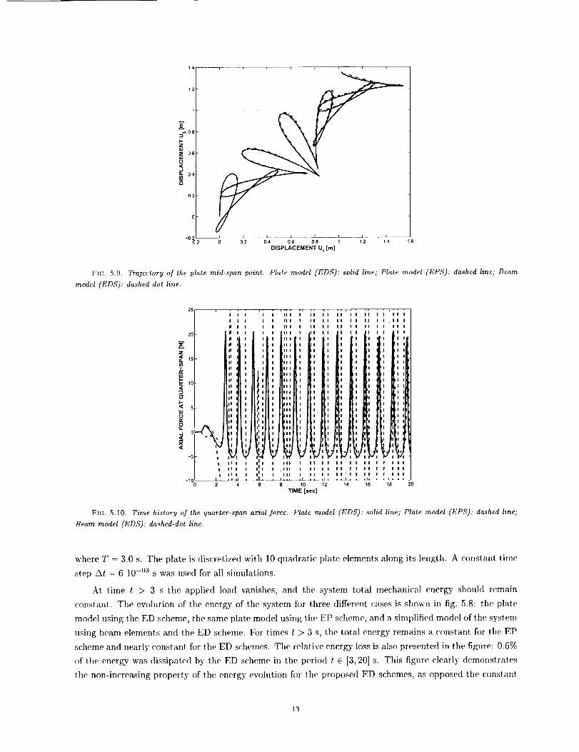
Fla. 5.9. Trajectory of the plate mid-span point+. Plate model (ED,q): solid line; Plate model (NPS): dashed line; Beam

model (EDS): dashed-dot line.

25 , -

20 II

tl

Z l*

Z iI

_D. 15 II

I II i

El

10

I| i

_I II I

(_ Inn

El II I

r_l II I

e,,,. ill0It. /'_ ill I

...j 0 "<_ _. ii iIpli

-5 I

t ||

I II I

.... t t',._2

I II I

I 11 I

III

III

III

III

III

III

III

III I

III I

III

I1|

III

III

r I II I I

III

III I

III

ill I

I

!

I

I I+I

I I

I

I

I

I

[I t

I III I I !

It III ! II I I

III III I II I+I

6 8 10 12

TIME [sec]

I II I I i II 1

1 I II 1

I 1 II I

! I

I I

I I

I I

I I

I I

I I

I I

I I

I I

I I

I I

I I

I I

I I

!, II! !

i,

j: jU I I II I

I I I I I

,,;,, ,/ ,,I4 16 18

I

II

I

I I

I I

I II

I II

I II

I II

I II

I II

I II

I II

I II

II II

to al

,',]i,

I 1

I I

| | |

20

FI,_,. 5.10. Time history of the quarter-span azial force. Dlate model (EDS): solid line; Plat+e model (EP,q): dashed line;

Beam model (EDS): dashed-do+ line.

where T = 3.0 s. The plate is discretized with 10 quadratic plate elements along its length. A constant time

step At = 6 10 -°'_ s was used for all simulations.

At time t > 3 s the applied load vanishes, and the system total mechanical energy should remain

constant. The evohltion of the energy of the system for three different cases is shown in fig. 5.8: the plate

model using the ED scheme, the same plate model using the EP scheme, and a simplified model of the system

using beam elements and the ED scheme. For times t > 3 s, the total energy remains a constant for the EP

scheme and nearly constant for the ED schemes. The relative energy loss is also presented in the figure: 0.6_

of the energy was dissipated by the ED scheme in the period t E [3, 20] s. This figure clearly demonstrates

the non-increasing property of the energy evolution for the proposed ED schemes, as opposed the constant

13

5-----

t|l d

0 _

o w., _._: _,:',' ,,' ,,_ ,' , V , h.

!:;_ ,_: ,,0 ",_,. ,,oIii I1 iiiii tl

" ,'. '% ,'I,Jh l

o 2 4 6

I

ITIME [sec]

Fit-;. 5.1 1. Time history of the q_tart, er-span transverse shear force. Plate model (EDS}: solid line," Plate model (EPS}:

dashed line; Beam model (EDS}: dashed-dot line.

energy predicted in EP simulations. The trajectory of the plate mid-span point is shown in fig. 5.9: good

correlation is observed between the predictions of the three models. The beam model is slightly off due to the

inherent simplifying assumptions. The behavior of the quarter-span axial force and transverse shear force

are shown in fig. 5.10 and 5.11, respectively. The poor predictions of the EP schemes are obvious in these

two plots. The history of axial force presents violent oscillations with amplitudes an order of magnitude

larger than those observed for the ED scheme. The history of the transverse shear force predicted by the

EP scheme quickly diverges from the ED predictions for both beam and plate models. To ascertain the

accuracy of the ED predictions, a convergence study was performed. Nearly identical results were found

with smaller time step sizes At = 3.0 and 1.0 10 o._ s, or when using the time adaptivity procedure. On

the other hand, oscillations of increasing amplitude were found as the time step size is reduced in the EP

scheme. Furthermore, the time adaptivity procedure failed to yield any results because the time step size

was driven to unreasonably small values, At = 10 -07 S, as the procedure tries to cope with increasingly

violent oscillations.

14

B_ki3

L_ .....

FI(;. 5.12. Configuration of the cruciform problem.

t=0.062 sec.

±, j

FIe.. 5.12. Configuration of the cruciform at times t = 0.062 and 0.093 s.

5.3. Dynamic Response of a Cruciform. Consider a cruciform consisting of four thin panels (Panels

A, B, C, and D) connected to a central beam, as depicted in fig. 5.12. Each panel is of thickness t = 4 ram,

length L = 1.2 m, and width b = 0.1 m. The central beam has a square cross-section of width a = 8 ram.

A mass M = 12 kg is attached at the tip of the central beam at point T. Panels and beam are simply

supported at the root of the cruciform. A concentrated load P(t) is applied at point T. The load acts in

the plane defined by axes i2 and i3 and makes a 30 degree angle with axis i2. All components are made of

aluminum with properties given in the previous example. The time history of the applied load is

P0 (1 - eos2rrt/T)/2 t <_ T, (5.3)P(t)

t 0 t>T,

where Po = 1.2 kN and T = 0.1 s.

As the applied load increases, in-plane stresses in the panels rapidly increase and buckling takes place

in those panels subjected to compression, as can be observed in fig. 5.13 that. depicts the configuration of

tile cruciform at two instants in time. The trajectory of point T projected onto plane i2, i3 is shown in

fig. 5.14. For reference, the corresponding trajectory of a beam with cross-sectional properties equivalent to

those of the cruciform is also presented. Of course, the equivalent beam model is much stiffer since it does

not allow buckling to take place. Furthermore, the motion remains confined to the plane defined by axis _1

and the line of action of the applied load. When each panel is modeled individually, the stiffness of system

15

0 05 --

o 04

o 03

2 002

001WU

o

-001

-002

-003-004

t I I t ......... J ......-002 0 0 02 0 04 0 06 008

DISPLACEMENT U z [m]

FIG. 5.14. Trajectory of point T of the cruciform projet:t, ed in the plane i_,2, i3. Solid line: shell model; dashed line: beam

model.

800

70O

600

_s0O

w 4OO

1-

20O

100

0002 0.04 006 008 01 012 014 0_6 018 02

TIME [sec]

F1G. 5.15. Total mechanical energy of the .system. Solid line." shell model; da.shed line: beam model.

varies both spatially and temporally, giving rise to the more complex motion shown in fig. 5.14. The total

mechanical energy of the system is shown in fig. 5.15. From time t. = 0.1 to 0.2 s, the system is free and

its total mechanical energy should remain constant. Due the dissipative nature of the integration scheme, a

small amount of energy is dissipated over that period of time: 2.7% of the energy was dissipated over the

2435 time step period.

The root shear force and quarter-span bending moment in Panels A and C are shown in fig. 5.16

and 5.17, respectively. E_ch panel undergoes alternating phases of tensile and compressive loading. During

the compressive phases, buckling takes place, and large shear forces and bending moments are ohserved in

contrast with the tensile phases during which these quantities remain much smaller.

16

x 10515 i

u.

_ 05

m

uJ

!o0O5

I tl

! ! I

L

0.02

!

004 006 0.0e 01 012 0• 4 016

TIME [see]

0118 02

FIG. 5,16. Time history of the root shear force in. Panel A (.solid line) and Panel C (dashed line).

150C

I00C

Z

5

£3

,,=,CD

50 ¸

w,,141

_ -I00C

0

-1500

-200_

q _ t _ t i q D

t I ..... ,_L__ • l l .... lJ- 0 I16 n002 004 0.06 008 01 012 0 4 018 02

TIME [see]

FT+. 5.17. Time history of the quarter-span bendin.q moment in Panel A (solid line) and Panel C (dashed line).

17

FIG. 5.18. Configuration of the snap-through problem.

=

T

t = 0.06 [sec] t t = 0.12 [sec]

_" t = 0.18 [sec] t = 0.24 [sec]

FIG. 5.19. System configurations at various time instants during the simulation.

5.4. Snap-Through of a Cylindrical Shell. The snap-through behavior of a cylindrical shell under

a concentrated load was investigated in ref [22]. The shell consists of a 60 degree sector of a cylinder of

height h = 5 m, radius R = 5 m and thickness t = 0.1 m, as shown in fig. 5.18. Malerial properties are:

Young's modulus E = 210 GPa, Poisson ratio v = 0.25 and density p = l04 kg/m '_. The two straight edges

of the shell are simply supported, while the two curved edges are free.

A concentrated force F is applied at the shell's apex. This force linearly increases from 0 to 5 107 N in

0.2 s, then is held constant at that value. The simulation ends at time t = 0.3 s. Due to the symmetry of

the problem, a quarter shell only is modeled; a regular 4 x 4 mesh of quadratic elements was used. The time

step size was selected as At = 10 -a s.

As the load increases, the shell apex displacement increases, then suddenly, snap-through takes place

and cm'vature reverses. Curvature reversal initiates in the region of the applied load, then quickly propagates

18

I--Z

lUO

5¢D

_0,,

g0 06

_04

0.2

t

/

I ! !

0O5 01 015 O2

TIME [sec]

__J= ....

0 25

FIG 5.20. Time history of the plate center vertical displacement. ED scheme." solid line," EP scheme: dashed line.

1

E

to

-2

o

Z

I/dI-

-7

x 10_

005 01 0 5 2

TIME [sec]

025

FIG. 5.21. Time history of the plate center forces .for the ED and EP schemes. Force F1 : solid line; F3: dashed line. For

clarity the EP results are shifted downwards 3 |08 N.

throughout the entire structure, whi(:h undergoes subsequent violent oscillations. Snapshots of the system

at various instants in time are given in fig. 5.19. The vertical displacements of the point of application of the

load computed with the ED scheme is shown in fig. 5.20. Note the gradual increase of the shell deflection,

until collapse at buckling and the resulting vibratory response in the inverted configuration.

Ref. [22] presents simulations of this problem using various schemes: the generalized-o [19] and the

CEMA [22] schemes. The former scheme features high frequency numerical dissipaHon and linear stability

properties, while the latter adds to the generalized-c_ method a constraint on the total mechanical energy of

the system. CEMA is therefore b()th energy preserving and high frequency dissipatiw_. The results presented

in fig. 5.20 are in (:lose agreement with those obtained with the generalized-c_ scheme, but quite different

19

200

i0

-200

W

-400

=zu

-600

-800

A

D 05

!

| ! t

f,

0 1 015 02 025

TIME [sec]

Ffc;. 5.22. Time history of the plate center vertical velocity. ED scheme: .solid line; EP scheme: dashed line, .shifted

downwards 3 102 m/s for clarity.

from those predicted by CEMA in the post buckling regime. It is important to realize that the higher

modes are only an artifact of the discretization process, and should therefore be removed from the computed

response. A standard scheme like the generalized-c, method accomplishes this goal through the characteristic

low-pass shape of its spectral radius; however, there is no guarantee that energy will not be allowed to grow

within one step for nonlinear problems. In contrast, CEMA enforces the exact conservation of energy in the

nonlinear regime, but at the same time inherits high frequency dissipation from the underlying generalized-c,

algorithm. Consequently, an artificial mechanism for transferring energy from the higher (artificial) modes

to the lower modes is created that drives the response to an erroneous solution. In contrast, the proposed

ED scheme achieves both nonlinear stability and high frequency dissipation.

Next, the same problem was simulated with p_ = 1, i.e. with no high frequency dissipation. In this

case, two refinements in time step size were required to successfully complete the simulation, one at time

t = 0.1665 s (At = 5 10 -4 S), the other at time t = 0.2142 s (At = 2.5 10- _ s). Deflections predicted

by the EP and ED schemes, shown in fig. 5.20, are in good agreement during the initial snap-through

phase, but become increasingly different during the subsequent oscillations. The force and velocity fields

are markedly different. The plate center forces for both EP and ED schemes are shown in fig. 5.21. The

forces predicted by the EP scheme present violent oscillations of amplitude up to an order of magnitude

larger than those predicted by the ED scheme. These violent oscillations hamper the convergence of the

Newton process at each time step, leading to the need for smaller time steps. The same observations can

be made about fig. 5.22 which compares the plate center vertical velocity. Violent oscillations are initiated

at snap-through and the strict preservation of energy implied by the EP scheme prevents any subsequent

decay of these vibrations. Since vibratory stresses are a great importance to designers, it is essential to

assess the ability of new integration schemes to reliably predict these quantities. It is unfortunate that many

scientific publications about geometric integration only present responses for preserved quantities such as

total mechanical energy or momentum. The above plots demonstrate that while EP scheme might perfi_rm

very well for the prediction of total energy, momentum, or even displacement fields, they are unable to

reliably predict other important fields such as velocities and internal stresses. Consequently, such schemes

20

areoflittle valuesin reallifeapplications.

6. Conclusions.In thiswork,arolmst_algorithmforthedynamicanalysisofgeometricallyexactshellstructureswaspresented.Themethodis geometry-based,i.e. it incorporates knowledge about specific

qualitative features of the underlying partial differential equations. However, departing from the classical

approaches based on strict preservation of energy, the method presented here allows the system to drift away

flom the level set of constant energy in a controlled and tunable manner.

This feature achieves two goals. First, a bound is placed on the total mechanical energy of the discrete

system, leading to the concept of nonlinear unconditional stability; this stability criterion is stronger than

that obtained through the classical analysis of numerical schemes. The resulting numerical procedure is

endowed with superior robustness, an important feature when dealing with complex engineering problems.

Second, the monotonic energy drift is associated with numerical dissipation of the high frequency modes.

This tunable dissipation makes the algorithm stiffly accurate, and avoids the build up of energy in the higher

modes that are an artifact of the spatial discretization process.

The proposed scheme can deal with general shell structures and is not tied to a specific spatial dis-

cretization of the governing partial differential equations. Kinematic nonlinearities are treated in a rigorous

manner, and material nonlinearities can be handled when the constitutive laws stem front the existence of a

strain energy density flmction. The efficiency and robustness of the proposed approach were demonstrated

with specific mlmerical examples.

REFERENCES

[9] O.

[10] O.

[1] K. BATHE AND E. DVORKIN, A four-node plate bending element based on mindlin/reissner plate theory

and a mixed interpolation, International Journal for Numerical Methods in Engineering, 21 (1985),

pp. 367- 383.

[2] --, A formulation of general shell elements - the use mixed interpolation o] tensorial components,

International Journal for Numerical Methods in Engineering, 22 (1986), pp. 697 722.

[3] O. BAUCHAU, Computational schemes for flexible, nonlinear multi-body systems, Multibody System

Dynamics, 2 (1998), pp. 169 225.

[4] ---, On the modeling of friction and rolling in flexible multi-body systems, Multibody System Dynam-

its, 3 (1999), pp. 209 239.

[5] --, Analysis of flexible multi-body systems with intermittent contacts, Multibody System Dynamics,

4 (2000), pp. 23 54.

[6] O. BAUCHAU AND C. BOTTASSO, On the design of energy preservin.q and decaying schemes for flexible,

nonlinear multi-body systems, Computer Methods in Applied Mechanics and Engineering, 169 (1999),

pp. 61 79.

[7] --, Robust integration schemes for flexible multibody systems, Computer Methods in Applied Me-

chanics and Engineering, (2000).

[8] O. BAUCttAU, J. CHOI, AND C. BOTTASSO, On the modeling of shells in multibody dynamics, Multibody

System Dynamics, (2000).

BAUCHAU AND T. Joo, Computational schemes for nonlinear elasto-dynamics, International Journal

for Numerical Methods in Engineering, 45 (1999), pp. 693 719.

BAUCHAU AND N. THERON, Enerqy decaying scheme for non-linear beam models, Computer Methods

in Applied Mechanics and Engineering, 134 (1996), pp. 37 56.

21

[13] V.

[141C.

[151--

[16] C.

[17] M.

[181 C.

[19] J.

[20] H.

[21] T.[221D.

[231a.

[241--

[251J.

[261 J.

--, Energy decaying schemes for nonlinear elastic multi-body systems, Computers and Structures, 59

(1996), pp. 317 331.

BORRI, C. BOTTASSO, AND L. THAINELLI, A novel momentum-preserving energy-decaying algo-

rithm for finite element multibody procedures, in Proceedings of Computational Aspects of Nonlinear

Structural Systems with Large Rigid Body Motion, NATO A(tvanced Research Workshop, Pullusk,

Poland, July 2-7, 2000.

BORRI, L. TRAINEI,IA, AND C. BOTTASSO, On representations and parameterizatious of motion,

Multibody Systems Dynamics, 4 (2000), pp. 129 193.

BOTTASSO AND ]'Vl. BORRI, Energy preserving/decaying schemes for non-linear beam dynamics using

the helicoidal approximation, Computer Methods in Applied Mechanics and Engineering, 143 (1997),

pp. 393 415.

., Integratin 9 finite rotations, Computer Methods in Applied Mechanics and Engineering, 164

(1998), pp. 307 331.

BOTTASSO, 1_,'[. B()RRI, ANI) L. TRAINELLI, Integration of elastic multibody systems using invariant

preserving/dissipating schemes. Part I formulation g_ Part H numerical schemes and applications.,

Computer Methods in Applied Mechanics and Engineering, (2000).

BUCAI,EM AND K. BATHE, Higher-order mite general shell elements, International Journal for

Numerical Methods in Engineering, 36 (1993), pp. 3729 3754.

BUDD AND A. ISERLES, Geometric integration: Numerical solution of differential equations on man-

ifolds, Philosophical Transactions of the Royal Society of London Series A-Mathematical Physical

and Engineering Sciences, 357 (1999), pp. 945 956.

CHUNG AND G. HUI,BERT, A time integration algorithm for structural dynamics with improved

numerical dissipation: The generalized-a m.ethod, Journal of Applied Mechanics, 122 (1995), pp. 254

266.

HILBER, T. HUGHES, AND R. TAYLOR, Improved numerical dissipation for time integration algo-

rithms in structural dynamics, Earthquake Engineering and Structural Dynamics, 5 (1977), pp. 282-

292.

KANE AND D. LEVINSON, Dynamics: Theory and Applications, McGraw-Hill, Inc., New York, 1985.

KU'HL AND R. E., Constraint energy momentum algorithm and its application to non-linear dynamics

of .shells, Computer Methods in Applied Mechanics and Engineering, 136 (1996)_ pp. 293 315.

SIMO AND N. TARNOW, The discrete energy-momentum method, conserving algorithms for nonlinear

dynamics, ZAMP, 43 (1992), pp. 757-792.

•, A..new energy and momentum conserving algorithm for the nonlinear dynamics of .shells, Inter-

national Journal for Numerical Methods in Engineering, 37 (1994), pp. 2527 2549.

SIMO, N. TARNOW, AND M. DOBLARE, Non-linear dynamics of three-dimensional rods: Exact energy

and momentum conserving algorithm.s, International Journal of Numerical Methods in Engineering,

38 (1995), pp. 1431 1473.

SIMO AND K. WON(;, Unconditionally stable algorithms for rigid body dynamics that exactly preserve

energy and momentum, International Journal for Numerical Methods in Engineering, 31 (1991),

pp. 19 52.

22

Appendix A. RodriguesParameters.A commonrepresentationof finiterotations[21]is in termsof Rodriguesparametersr_ = 2k_ tall 0/2,

where ¢ is the magnitude of the finite rotation and L the components of the unit vector about which it takes

place. The following notation is introduced r0 = cos 2 0/2 = l / (1 + Lr g/4), and the finite rotation tensor

R then writes

ro _ (A.1)R(r) = [ + ro "r + -_ rr.

The following decomposition of the rotation tensor is extensively used in this work

= + + + + ; =----7. (A.2)

Appendix B. Orientation of a Unit Director.

Consider a unit vector k3, called a director, that rotates to a final orientation £a. For convenience, this

director is considered to be tile third unit vector of a triad S defined by il, i'2, i3, rotating to a. triad S* with

orientation el, £.9, Ca. The relationship between these two triads is e_ = R _a, where R is an orthogonal

rotation tensor. If one solely focuses on the director, this rotation tensor is not. uniquely defined, as any

rotation about the director leaves its orientation unchanged. A virtual change in the director orientation is

where 5_) is the virtual rotation vector, &b = aRR r.

The components of the virtual change in director orientation measured in S* become

(B.1)

(B.2)0

where 5_* are the components of the virtual rotation vector in ,5*. This relationship clearly demonstrates

that arbitrary vahms of a_b._, corresponding to virtual rotations of the director about its own orientation,

will not affect virtual changes in the director orientation, and hence, setting _._ = 0 is a valid choice. The

&b" = z_,aa_ +i2ac,_ = b&**; b = [i,,/2]. (B.3)

following notation is adopted

a_.o_a*is a 2 x 1, "two parameter" virtual rotation vector. It follows that 5_____= R 5gJ* = Rb 5____o*,and hence

ae,__= R .-'r,ab &_*. (B.4)

If R odrigues parameters are used to parameterize R, an equivalent expression can be obtained for finite

changes in director orientation with the help of eq. (A.2)

eal - _e_i = R,, _ b s* = s* r__* s*,o _ O,,,_ ; = b_, (n.5)

where r_*are the Rodrigues parameter measured in ,5", and ._s*the corresponding "two parameter" incremental

rotation vector.

23

I Form ApprovedREPORT DOCUMENTATION PAGE OMBNo 0704-0188

Public repotting burden for this coffect;on of information ;S estimated to average ] hour per response, including the t;rne for reviewing instructions, searching existing data sources,gathering and mainta;nlng the data needed, and completing and reviewing the collection of" in{otmatlon Send comments regarding this burden estimate or any other aspect of thisco}lectlon of information, _ncludlng suggestions for reducing this burden, to Washington Headquarters Services. D_rectorate f'or Informal;on Operations at_d Reports, 1215 JeffersonDavis Highway. Suite 1204, Arlington,VA 22202 4302, and to the OfFice of Management and Budget, Paperwork Reduction Project (0704 0188), Washington, t')C 20503

1. AGENCY USE ONLY(Leave blank) 2. REPORT DATE 3. REPORT TYPE AND DATES COVERED

November 2000

4. TITLE AND SUBTITLE

An energy decaying scheme for nonlinear dynamics of shells

6. AUTHOR(S)

Carlo L. Botta.sso, Olivier A. Bauchau, and Jou-Young Choi

7. PERFORMING ORGANIZATION NAME(S) AND ADDRESS(ES)

ICASE

Mail Stop 132C

NASA Langley Research Center

Hampton, VA 23681-2199

9. SPONSORING/MONITORING AGENCY NAME(S) AND ADDRESS(ES)

National Aeronautics and Space Administration

Langley Research Center

Hampton, VA 23_681-2199

Contractor Report

5. FUNDING NUMBERS

C NASI 97046

WU 505-90-52 01

8. PERFORMING ORGANIZATION

REPORT NUMBER

ICASE Report No. 2000 43

10. SPONSORING/MONITORING

AGENCY REPORT NUMBER

NASA/CR-2000 210557ICASE Report No. 2000 43

11. SUPPLEMENTARY' NOTES

Langley Technical Monitor: Dennis M. Bushnell

Final Report

Submitted to Computer Methods in Applied Mechanics and Engineering.

12a. DISTRIBUTION/AVAILABILITY STATEMENT

Unclassified Unlimited

Subject Category 64Distribution: Nonstandard

Availability: NASA-CASI (301) 621 0390

12b. DISTRIBUTION CODE

13. ABSTRACT (Maximum 200 words)

A novel integration scheme for nonlinear dynamics of geometrically exact shells is developed based on the inextensible

director assumption. The new algorithm is designed so as to imply the strict decay of the system total mechanicalenergy at each time step, and consequently unconditional stability is achieved in the nonlinear regime. Furthermore,

the scheme features tunable high frequency numerical damping and it is therefore stiffly accurate. The method is

tested for a finite element spatial formulation of shells ba.sed on mixed interpolations of strain tensorial componentsand on a two-parameter representation of director rotations. The robustness of the schelne is ilhlstrated with the

help of numerical examples.

14. SUBJECT TERMS

geometrically exact shell, time integration, energy decaying scheme

17. SECURITY CLASSIFICATION

OF REPORT

Unclassified

_ISN 7540-01-280-5500

18. SECURITY CLASSIFICATION

OF THIS PAGE

Uncla._sified

19. SECURITY CLASSIFICATION

OF ABSTRACT

1S. NUMBER OF PAGES

28

16. PRICE CODE

A0320. LIMITATION

OF ABSTRACT

iStandard Form 298(Rev. 2-89)Prescribed by ANSI Std Z39 18298-102