Embed Size (px)
Citation preview

A REAL-TIME ITERATION SCHEME FOR NONLINEAROPTIMIZATION IN OPTIMAL FEEDBACK CONTROL∗
MORITZ DIEHL† , HANS GEORG BOCK† , AND JOHANNES P. SCHLODER†
SIAM J. CONTROL OPTIM. c© 2005 Society for Industrial and Applied MathematicsVol. 43, No. 5, pp. 1714–1736
Abstract. An efficient Newton-type scheme for the approximate on-line solution of optimizationproblems as they occur in optimal feedback control is presented. The scheme allows a fast reactionto disturbances by delivering approximations of the exact optimal feedback control which are it-eratively refined during the runtime of the controlled process. The contractivity of this real-timeiteration scheme is proven, and a bound on the loss of optimality—compared with the theoreticaloptimal solution—is given. The robustness and excellent real-time performance of the method isdemonstrated in a numerical experiment, the control of an unstable system, namely, an airborne kitethat shall fly loops.
Key words. direct multiple shooting, Newton-type optimization, optimal feedback control,nonlinear model predictive control, ordinary differential equations, real-time optimization
AMS subject classifications. 34B15, 34H05, 49N35, 49N90, 90C06, 90C30, 90C55, 90C59,90C90, 93C55
DOI. 10.1137/S0363012902400713
1. Introduction. Feedback control based on the real-time optimization of non-linear dynamic process models, also referred to as nonlinear model predictive con-trol (NMPC), has attracted increasing attention over the past decade, particularly inchemical engineering [4, 27, 1, 28]. Based on the current system state, feedback isprovided by an online optimization of the predicted system behavior, using the math-ematical model. The first part of the optimized control trajectory is implemented atthe real system, and a sampling time later the optimization procedure is repeated.Among the advantages of this approach are the flexibility provided in formulatingthe objective and in modeling the process using ordinary or partial differential equa-tions (ODEs or PDEs), the capability of directly handling equality and inequalityconstraints, and the possibility of treating large disturbances quickly.
One important precondition, however, is the availability of reliable and efficientnumerical optimal control algorithms. One particularly successful algorithm that isdesigned to achieve this aim, the recently developed real-time iteration scheme, willbe the focus of this paper. In the literature, several suggestions have been madeon how to adapt off-line optimal control algorithms for use in on-line optimization.For an overview and comparison of important approaches, see, e.g., Binder et al. [6].We particularly mention here the “Newton-type control algorithm” proposed by Liand Biegler [32] and de Oliveira and Biegler [15] and the “feasibility-perturbed SQP”approach to NMPC by Tenny, Wright, and Rawlings [38]. Both approaches keep evenintermediate optimization iterates feasible. This is in contrast to the simultaneousdynamic optimization methods, as the collocation method proposed in Biegler [5] orthe direct multiple shooting method in Bock et al. [7] and in Santos [37], which allow
∗Received by the editors July 30, 2002; accepted for publication (in revised form) April 12, 2004;published electronically March 11, 2005. This work was supported by the Deutsche Forschungsge-meinschaft (DFG) within the priority program 469 “Online-Optimization of Large Scale Systems”and within the research project “Optimization Based Control of Chemical Processes.”
http://www.siam.org/journals/sicon/43-5/40071.html†Interdisciplinary Center for Scientific Computing (IWR), University of Heidelberg, Im Neuen-
heimer Feld 368, 69120 Heidelberg, Germany ([email protected], [email protected], [email protected]).
1714
REAL-TIME ITERATIONS FOR OPTIMAL FEEDBACK CONTROL 1715
infeasible state trajectories and are more suitable for trajectory following problemsand problems with final state constraints. The real-time iteration scheme belongs tothis latter class.
Most approaches in the literature try to solve quickly but exactly an optimalcontrol problem. However, if the time scale for feedback is too short for exact compu-tation, some approximations must be made: for this aim an “instantaneous control”technique has been proposed in the context of PDE models that approximates theoptimal feedback control problem by regarding one future time step only (Choi etal. [14, 13]). By construction, this “greedy” approach to optimal control is based onimmediate gains only and neglects future costs; thus it may result in poor perfor-mance when future costs matter. A somewhat opposed approach to derive a feedbackapproximation (formulated for ODE models) is based on a system linearization alonga fixed optimal trajectory over the whole time horizon and can, e.g., be found inKramer-Eis and Bock [29] or Kugelmann and Pesch [30]. The approach works wellwhen the nonlinear system is not too largely disturbed and stays close to the nominaltrajectory.
The real-time iteration scheme presented in this paper is a different approximationtechnique for optimal feedback control. It regards the complete time horizon and per-forms successive linearizations along (approximately) optimal trajectories to providefeedback approximations. Using these linearizations, it iterates toward the rigorousoptimal solutions during the runtime of the process. In this way a truly nonlinearoptimal feedback control is provided whose accuracy is limited, however, by the timeneeded to converge to the current optimal solutions. In contrast to a somewhat similaridea mentioned in [32], the real-time iteration scheme is based on the direct multipleshooting method [12], a simultaneous optimization technique, which offers excellentconvergence properties, particularly for tracking problems and problems with stateconstraints.
The scheme was introduced in its present form in Diehl et al. [19] going back toideas presented in Bock et al. [10]. In its actual implementation it is able to treatdifferential algebraic equation (DAE) models (Leineweber [31]), as they often arisein practical applications. It has already been successfully tested for the feedbackcontrol of large-scale DAE models with inequality constraints, particularly a binarydistillation column [11, 33, 19]. Moreover, it has been applied for the NMPC of areal pilot plant distillation column situated at the Institut fur Systemdynamik undRegelungstechnik (ISR) of the University of Stuttgart [25, 16, 21].
However, to concentrate on the essential features of the method and on a newproof of contractivity of the scheme, we will restrict the presentation in this paper toODE models and optimization problems of a simplified type. Moreover, we will startthe paper by regarding (nonlinear) discrete-time systems first; the multiple shootingtechnique, which allows us to formulate a discrete-time system from an ODE system,is only introduced later, and very briefly, when the numerical example is presented.Part of the material is also covered in [18]; for technical details about the real-timeiteration scheme we refer to [16, 20].
1.1. Real-time optimal feedback control. Throughout this paper, let usconsider the simplified nonlinear controlled discrete-time system
xk+1 = fk(xk, uk), k = 0, . . . , N − 1,(1.1)
with system states xk ∈ Rnx and controls uk ∈ R
nu . The aim of optimal feedbackcontrol is to find controls uk that depend on the current system state xk and that are

1716 M. DIEHL, H. G. BOCK, AND J. P. SCHLODER
qk
qk+1qk+2
qN−1�
�
�
�
�
�
�
�
�
�
�
�
�
�
�
�
�
�
�
�
sk sk+1sk+2
sk+3
�xk
sN−1
�sN
fN−1(sN−1, qN−1)
� � � � ��
Fig. 1.1. Problem Pk(xk): Initial value xk and problem variables sk, . . . , sN and qk, . . . , qN−1.
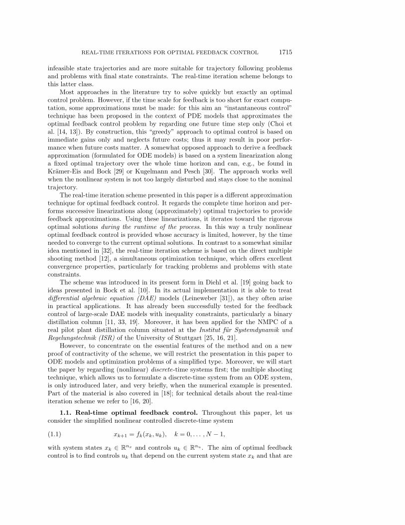
optimal with respect to a specified objective. As time advances, we proceed by solvinga sequence of nonlinear programming problems Pk(xk) on shrinking horizons, eachwith the current system state xk as initial value (for a visualization, see Figure 1.1).Let us define Pk(xk) to be the problem
minsk, . . . , sN ,
qk, . . . , qN−1
N−1∑i=k
Li(si, qi) + E(sN )(1.2a)
subject to
xk − sk = 0,(1.2b)
fi(si, qi) − si+1 = 0, i = k, . . . , N − 1.(1.2c)
The control part (q∗k, . . . , q∗N−1) of the solution of problem Pk(xk) allows us to define
the optimal feedback control
uk := q∗k.
Note that, due to the dynamic programming property, the optimal control trajectory(q∗0 , . . . , q
∗N−1) of the first problem P0(x0) would already give all later closed-loop
controls u0, u1, . . . uN−1, if the system behaves as predicted by the model. The prac-tical reason to introduce the closed-loop optimal feedback control is, of course, thatit allows us to optimally respond to disturbances.
We will now assume that we know each initial value xk only at the time when thecorresponding control uk is already needed for application to the real process, andthat the solution time for each problem Pk(xk) is not negligible compared with theruntime of the process. This is a typical situation in realistic applications: ideally,we would like to have the solution of each problem Pk(xk) instantaneously, but dueto finite computing power this usually cannot be accomplished in practice. In thispaper we propose and investigate an efficient Newton-type scheme that allows us toapproximately solve the optimization problems Pk(xk) during the runtime of the realprocess.
Remark. In practical applications, inequality path constraints of the formh(si, qi) ≥ 0, like bounds on controls or states, are of major interest and are usu-ally present in the formulation of the optimization problems Pk(xk). For the purposeof this paper we leave such constraints unconsidered, since general convergence resultsfor Newton-type methods with changing active sets are difficult to establish. However,we note that in the practical implementation of the real-time iteration scheme theyare included and pose no difficulty for the performance of the algorithm.
REAL-TIME ITERATIONS FOR OPTIMAL FEEDBACK CONTROL 1717
1.2. Overview. The paper is organized as follows:• In section 2 we give a review of Newton-type optimization methods for the
solution of optimal control problems of type (1.2) and discuss the problemstructure.
• The real-time iteration scheme is presented in section 3 building on the pre-viously introduced Newton-type methods. It performs only one Newton-typeiteration per optimization problem Pk(xk), applies the obtained feedback con-trol to the real system, and then proceeds already to the following problem,Pk+1(xk+1), until the end of the horizon is reached. This allows a particularlyfast reaction to disturbances.
• A new contractivity result for the scheme is presented and proven in section 4.The theorem guarantees that the real-time iteration scheme is contractingunder mild conditions and delivers approximations to the optimal feedbackcontrol with diminishing error.
• Based on the contractivity result, a bound on the loss of optimality of thescheme compared to exact optimal feedback control is established in section 5.
• In section 6 we finally present a numerical example, the real-time control ofa kite that shall start to fly loops. A new kite model is developed and aperiodic reference orbit is defined. The optimal control problem is to steerthe kite into the periodic orbit, starting at an a priori unknown initial value.This example, though of small state dimension, is particularly challenging,because the system is highly nonlinear and unstable.
2. Newton-type optimization methods. In order to solve an optimizationproblem Pk(xk), let us first introduce the Lagrange multipliers λk, . . . , λN and definethe Lagrangian function Lk(λk, sk, qk, . . . ) of problem Pk(xk) to be
Lk(·) =∑N−1
i=k Li(si, qi) + E(sN ) + λkT (xk − sk) +
∑N−1i=k λi+1
T (fi(si, qi) − si+1).
Summarizing all variables in a vector y := (λk, sk, qk, λk+1, sk+1, qk+1, . . . , λN , sN ) ∈R
nk ,1 we can formulate necessary optimality conditions of first order (also calledKarush–Kuhn–Tucker conditions):
∇yLk(y) = 0.(2.1)
To solve this system, the exact full-step Newton–Raphson method would start at aninitial guess y0 and compute a sequence of iterates y1, y2, . . . according to
yi+1 = yi + ∆yi,(2.2)
where each ∆yi is the solution of the linearized system
∇yLk(yi) + ∇2yLk(yi)∆yi = 0.(2.3)
The Newton-type methods considered in this paper differ from the exact Newton–Raphson method in the way that a part of the exact second derivative ∇2
yLk, namely,
the Hessian ∇2(q,s)Lk, is replaced by a (symmetric) approximation. We denote the
resulting approximation of ∇2yLk(y) by Jk(y). For our Newton-type method, (2.3) is
replaced by the approximation
∇yLk(yi) + Jk(yi)∆yi = 0.(2.4)
1For simplicity, we omit the index k for the variable y and implicitly assume that y ∈ Rnk when
not specified otherwise. Note that nk = (2nx + nu)(N − k) + 2nx.
1718 M. DIEHL, H. G. BOCK, AND J. P. SCHLODER
The matrix ∇2yLk, respectively, its approximation Jk, is often referred to as the
Karush–Kuhn–Tucker (KKT) matrix.
2.1. Structure of the Karush–Kuhn–Tucker matrix. The Lagrangian func-tion Lk of the optimal control problem is partially separable [12], and its secondderivative has a block diagonal structure:
∇2yLk(y)=
⎛⎜⎜⎜⎜⎜⎜⎜⎜⎜⎜⎜⎜⎜⎜⎜⎜⎜⎜⎝
−I
−I Qk Mk ATk
MTk Rk BT
k
Ak Bk −I
−I Qk+1 Mk+1 ATk+1
MTk+1 Rk+1 BT
k+1
Ak+1 Bk+1
. . .
. . . QN−1 MN−1 ATN−1
MTN−1 RN−1 BT
N−1
AN−1 BN−1 −I
−I QN
⎞⎟⎟⎟⎟⎟⎟⎟⎟⎟⎟⎟⎟⎟⎟⎟⎟⎟⎟⎠
,
where we have set
Ai :=∂fi∂si
, Bi :=∂fi∂qi
,
(Qi Mi
MTi Ri
):= ∇2
(si,qi)Lk, and QN := ∇2
sNLk.
In the approximation Jk(y) of this second derivative, we replace Qi,Mi, and Ri byapproximations QH
i (si, qi, λk+1),MHi (si, qi, λk+1), and RH
i (si, qi, λk+1).Remark 1. Note that the KKT matrix of each problem Pk(xk) is completely
independent of the value of xk.Remark 2. If we split the variables y = (λk, sk, qk, . . . ) = (λk, sk, qk, y) into a
first and a second part, the second part y ∈ Rnk+1 corresponds directly to the variable
space of the next, shrunken problem Pk+1(xk+1), and we can see that the KKT matrixcontains the KKT matrix of the next problem as a submatrix, as
∇2yLk(y) =
⎛⎜⎜⎜⎜⎜⎜⎝
−I
−I Qk Mk ATk
MTk Rk BT
k
Ak Bk
∇2yLk+1(y)
⎞⎟⎟⎟⎟⎟⎟⎠
.
Remark 3. The favorable structure of the matrix ∇2yLk(y), respectively, its ap-
proximation Jk(y), allows an efficient solution of the linear system Jk(y)x = b bya Riccati recursion proposed independently by Pantoja [34] and Dunn and Bert-sekas [26]; cf. also [36, 16].
2.2. The constrained Gauss–Newton method. An important special case ofthe Newton-type methods considered in this paper is the constrained Gauss–Newtonmethod, which is applicable for problems with a least squares form of the objectivefunction
N−1∑i=k
1
2‖li(si, qi)‖2
2 +1
2‖e(sN )‖2
2.(2.5)

REAL-TIME ITERATIONS FOR OPTIMAL FEEDBACK CONTROL 1719
For this case, the Hessian block approximations QHi ,MH
i , and RHi are defined to be
(QH
i MHi
(MHi )T RH
i
):=
(∂li(si, qi)
∂(si, qi)
)T∂li(si, qi)
∂(si, qi), QH
N :=
(∂e(sN )
∂sN
)T∂e(sN )
∂sN.(2.6)
Note that these Hessian block approximations do not depend on the values of theLagrange multipliers.
2.3. Local convergence. It is well known that the Newton-type scheme (2.4)for the solution of (2.1) converges in a neighborhood Dk ⊂ R
nk of a solution yk∗that satisfies the second order sufficient conditions for optimality of problem Pk(xk)if Jk(y) approximates ∇2
yLk(y) sufficiently well on Dk.
3. Real-time iterations. Let us now go back to the real-time scenario describedin section 1.1, where we want to solve the sequence of optimization problems Pk(xk),but where we do not have the time to iterate each problem to convergence. Letus more specifically assume that each Newton-type iteration needs exactly as muchcomputation time as corresponds to the time that the real process needs for thetransition from one system state to the next. Thus, we can only perform one singleNewton-type iteration for each problem Pk(xk), and then we have to proceed already tothe next problem Pk+1(xk+1). The real-time iteration scheme that we will investigatehere is based on a carefully designed transition between subsequent problems. Afteran initial disturbance, it subsequently delivers approximations uk for the optimalfeedback control that become better and better if no further disturbance occurs, aswill be shown in section 4.
It turns out that the computations of the real-time iteration belonging to problemPk(xk) can largely be prepared without knowledge of the value of xk so that we canassume that the approximation uk of the optimal feedback control is instantly availableat the time that xk is known. However, after this feedback has been delivered, weneed to prepare the next real-time iteration (belonging to problem Pk+1(xk+1)) whichneeds the full computing time.
In the framework for optimal feedback control on shrinking horizons (1.2), wereduce the number of remaining intervals from one problem Pk(xk) to the nextPk+1(xk+1), in order to keep pace with the process development. Therefore, wehave to perform real-time iterates in primal-dual variable spaces R
n0 ⊃ · · · ⊃ Rnk ⊃
Rnk+1 ⊃ · · · ⊃ R
nN−1 of different sizes. Let us denote by Πk+1 the projection fromR
nk onto Rnk+1 ; i.e., if y = (λk, sk, qk, y) ∈ R
nk , then Πk+1y = y ∈ Rnk+1 .
3.1. The real-time iteration algorithm. Let us assume that we have an ini-tial guess y0 ∈ R
n0 for the primal-dual variables of problem P0(·). We set the iterationindex k to zero and perform the following steps:
1. Preparation. Based on the initial guess yk ∈ Rnk , compute the vector
∇yLk(yk) and the matrix Jk(yk): Note that Jk(yk) is completely independentof the value of xk, and that of the vector ∇yLk(yk) only the first component(∇λk
Lk = xk − sk) depends on xk. This component will only be neededin the second step. Therefore, prepare the linear algebra computation ofJk(yk)−1∇yLk(yk) as much as possible without knowledge of the value of xk
(a detailed description how this can be achieved is given in [19] or [16]).2. Feedback response. At the time when xk is exactly known, finish the com-
putation of the step vector ∆yk = −Jk(y)−1∇yLk(yk) and give the controluk := qk + ∆qk immediately to the real system.
1720 M. DIEHL, H. G. BOCK, AND J. P. SCHLODER
3. Transition. If k = N − 1, stop. Otherwise, compute the next initial guessyk+1 by adding the step vector to yk and “shrinking” the resulting variablevector onto R
nk+1 ; i.e., yk+1 := Πk+1(yk + ∆yk). Set k = k + 1 and go to 1.Note that after one iteration belonging to system state xk we expect the next systemstate to be xk+1 = fk(xk, uk), but this may not be true due to disturbances. Thescheme allows an immediate feedback to such disturbances, due to the separation ofsteps 1 and 2. This separation is only possible because we do not require the guessof initial value, sk, to be equal to the real initial value, xk. This formulation may beregarded as an initial value embedding of each problem into the manifold of perturbedproblems. Though this formulation comes quite naturally in the framework of aninfeasible path (also simultaneous) solution strategy, as presented, where optimalityand constraints are treated simultaneously, it deserves strong emphasis as it is afeature that is crucial for the success of the method in practice.
We will in the following investigate the contraction properties of the real-timeiteration scheme. Though a principal advantage of the scheme lies in this immediateresponse to disturbances, we will investigate contractivity only under the assumptionthat after an initial disturbance the system behaves according to the model. Thisis analogous to the notion of “nominal stability” for an infinite horizon steady statetracking problem.
4. Contractivity of the real-time iterations. In this subsection we investi-gate the contraction properties of the real-time iteration scheme. The system startsat an initial state x0, and the real-time algorithm is initialized with an initial guessy0 ∈ D0 ⊂ R
n0 . Let us define the projections Dk of the neighborhood D0 onto theprimal-dual subspaces R
nk ; i.e., Dk+1 := Πk+1Dk.We will in the following make use of vector and corresponding matrix norms ‖ ·‖k
defined on the subspaces Rnk . These norms are assumed to be compatible in the sense
that ‖Πk+1y‖k+1 ≤ ‖y‖k and that ‖Πk+1T y‖k = ‖y‖k+1.Theorem 4.1 (local contractivity of the real-time iterations). Let us assume that
the Lagrangian functions Lk : Dk → R for all k = 0, . . . , N are twice continuouslydifferentiable and that their second derivative approximations Jk : Dk → R
nk×nk arecontinuous and have a bounded inverse (Jk)−1 : Dk → R
nk×nk .Furthermore, let us assume that there exist a κ < 1 and an ω < ∞ such that for
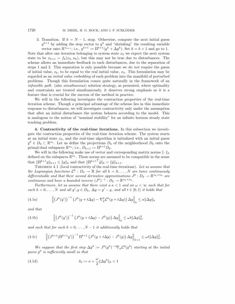
each k = 0, . . . , N and all y′, y ∈ Dk, ∆y = y′ − y, and all t ∈ [0, 1] it holds that∥∥∥(Jk(y′))−1 (
Jk(y + t∆y) −∇2yLk(y + t∆y)
)∆y
∥∥∥k≤ κ‖∆y‖k(4.1a)
and that ∥∥∥(Jk(y′))−1 (
Jk(y + t∆y) − Jk(y))∆y
∥∥∥k≤ ωt‖∆y‖2
k,(4.1b)
and such that for each k = 0, . . . , N − 1 it additionally holds that∥∥∥(Jk+1(Πk+1y′))−1
Πk+1(Jk(y + t∆y) − Jk(y)
)∆y
∥∥∥k+1
≤ ωt‖∆y‖2k.(4.1c)
We suppose that the first step ∆y0 := J0(y0)−1∇yL0(y0) starting at the initialguess y0 is sufficiently small so that
δ0 := κ +ω
2‖∆y0‖0 < 1(4.1d)

REAL-TIME ITERATIONS FOR OPTIMAL FEEDBACK CONTROL 1721
and that the ball
B0 :=
{y ∈ R
n0 | ‖y − y0‖0 ≤ ‖∆y0‖0
1 − δ0
}(4.1e)
is completely contained in D0. Under these conditions the real-time iterates y0, . . . , yN
defined by
∆yk := −Jk(yk)−1∇yLk(yk), yk+1 := Πk+1(yk + ∆yk)
(where Lk is the Lagrangian function corresponding to problem Pk(xk) with the systemstate obtained according to the closed-loop dynamics xk+1 = fk(xk, uk), uk := qkk +∆qkk) are well defined and stay in the projections of the ball B0, i.e.,
yk ∈ Πk · · ·Π1B0 ⊂ Dk,(4.2)
and satisfy the contraction condition
‖∆yk+1‖k+1 ≤(κ +
ω
2‖∆yk‖k
)‖∆yk‖k =: δk‖∆yk‖k ≤ δ0‖∆yk‖k.(4.3)
Furthermore, the iterates yk approach the exact stationary points yk∗ of the correspond-ing problems Pk(xk):
‖yk − yk∗‖k ≤ ‖∆yk‖k1 − δk
≤ (δ0)k‖∆y0‖0
1 − δ0.(4.4)
Proof. We divide the proof into three parts, corresponding to the properties(4.3), (4.2), and (4.4).
Contraction property. We will first show that the contraction property (4.3) holds.By adding zero to the defining equation of ∆yk+1 we get
−∆yk+1 = Jk+1(yk+1)−1∇yLk+1(yk+1)= Jk+1(yk+1)−1
(∇yLk+1(yk+1) − Πk+1
(∇yLk(yk) + Jk(yk)∆yk
)).
(4.5)
Using the notation yk = (λkk, s
kk, q
kk , λ
kk+1, s
kk+1, q
kk+1, . . . ) we observe that
∇yLk+1(yk+1) = ∇yLk+1(Πk+1(yk + ∆yk)) =
(xk+1 − (skk+1 + ∆skk+1)
...
)
=
(fk(s
kk+∆skk, q
kk+∆qkk) − (skk+1 + ∆skk+1)
...
)
= Πk+1∇yLk(yk + ∆yk),
because xk+1 = fk(xk, uk) = fk(skk+∆skk, q
kk +∆qkk) if the system was undisturbed.2
Therefore, we can continue to transform ∆yk+1 and write
−∆yk+1 = Jk+1(yk+1)−1Πk+1(∇yLk(yk + ∆yk) −∇yLk(yk) − Jk(yk)∆yk
)= Jk+1(yk+1)−1Πk+1
∫ 1
0(∇2
yLk(yk + t∆yk) − Jk(yk))∆yk dt
= Jk+1(yk+1)−1Πk+1∫ 1
0(∇2
yLk(yk + t∆yk) − Jk(yk + t∆yk))∆yk dt
+Jk+1(yk+1)−1Πk+1∫ 1
0(Jk(yk + t∆yk) − Jk(yk))∆yk dt.
(4.6)
2Note that skk+∆skk = xk due to the linearity of the constraint xk−sk = 0 and that uk = qkk+∆qkkby definition.

1722 M. DIEHL, H. G. BOCK, AND J. P. SCHLODER
Noting that, with y := Πk+1y,
Πk+1(∇2
yLk(y) − Jk(y))
= Πk+1
⎛⎜⎜⎜⎜⎜⎜⎝
00 ∆Qk ∆Mk 0
∆MTk ∆Rk 0
0 0
∇2yLk+1(y) − Jk+1(y)
⎞⎟⎟⎟⎟⎟⎟⎠
=
⎛⎜⎝
0 0 0...
...... ∇2
yLk+1(y) − Jk+1(y)0 0 0
⎞⎟⎠
and abbreviating yk := Πk+1yk, ∆yk := Πk+1∆yk, we can exploit assumption (4.1a)to obtain
‖Jk+1(yk+1)−1 Πk+1(∇2yLk(yk + t∆yk) − Jk(yk + t∆yk))∆yk‖k+1
= ‖Jk+1(yk+1)−1(∇2yLk+1(yk + t∆yk) − Jk+1(yk + t∆yk))∆yk‖k+1
≤ κ‖∆yk‖k+1 = κ‖Πk+1∆yk‖k+1 ≤ κ‖∆yk‖k.
Making also use of assumption (4.1c), we can, building on (4.6), prove the left in-equality of the contraction property (4.3):
‖∆yk+1‖k+1 ≤ κ‖∆yk‖k +
∫ 1
0
ωt‖∆yk‖2k dt. = κ‖∆yk‖k +
1
2ω‖∆yk‖2
k =: δk‖∆yk‖k.
With the help of condition (4.1d) (δ0 < 1) it is straightforward to deduce inductivelythat
δk+1 = κ +ω
2‖∆yk+1‖k+1 ≤ κ +
ω
2δk‖∆yk‖k ≤ δk ≤ δ0,
which proves the remaining part of (4.3).
Well definedness. To show that the iterates remain inside the domains of defini-tion as stated in (4.2) we first observe that
‖∆yk‖k ≤ δk−1δk−2 . . . δ0‖∆y0‖0 ≤ (δ0)k‖∆y0‖0.
Using the representation
yk = Πk(yk−1 + ∆yk−1) = Πk(Πk−1(yk−2 + ∆yk−2) + ∆yk−1)= Πk(Πk−1(. . .Π1(y0 + ∆y0) . . . ) + ∆yk−1)= Πk · · ·Π1y0 + Πk · · ·Π1∆y0 + · · · + Πk∆yk−1,
we can find y′ := y0 + (Πk · · ·Π1)T (yk − Πk · · ·Π1y0) such that
‖y′ − y0‖0 = ‖(Πk · · ·Π1)T (yk − Πk · · ·Π1y0)‖0 = ‖yk − Πk · · ·Π1y0‖k≤
∑k−1i=0 ‖∆yi‖i ≤ ‖∆y0‖0
∑k−1i=0 (δ0)
i ≤ ‖∆y0‖0
1−δ0,
i.e., y′ ∈ B0 and yk = Πk . . .Π1y′, i.e., yk ∈ Πk . . .Π1B0, as desired.
REAL-TIME ITERATIONS FOR OPTIMAL FEEDBACK CONTROL 1723
Distance to optimal solutions. It remains to be shown that the iterates yk ap-proach the exact solutions of the corresponding problems Pk(xk) as stated in (4.4).For this aim we devise a hypothetical standard Newton-type algorithm as introducedin (2.4) that allows us to compute the exact solution yk∗ of Pk(xk). As a by-product,we obtain a bound on the distance of yk∗ from yk.
The hypothetical algorithm would proceed by starting at yk0 := yk and iteratingwith iterates yk1 , y
k2 , . . . according to
yki+1 := yki + ∆yki , ∆yki := −Jk(yki )−1∇yLk(yki ).
Note that the first step ∆yk0 is identical to ∆yk. It is for this hypothetical algorithmonly that we need assumption (4.1b). Due to this condition and (4.1a), we have thecontraction property
‖∆yki+1‖k ≤(κ +
ω
2‖∆yki ‖k
)‖∆yki ‖k
as can be shown by a well-known technique for Newton-type methods (see, e.g., [9]):
‖∆yki+1‖k = ‖Jk(yki+1)−1 · ∇yLk(yki+1)‖k
= ‖Jk(yki+1)−1 · (∇yLk(yki+1) −∇yLk(yki ) − Jk(yki ) · ∆yki )‖k
= ‖Jk(yki+1)−1 ·
∫ 1
0(∇2
yLk(yki + t∆yki ) − Jk(yki )) · ∆yki dt‖k= ‖Jk(yki+1)
−1 ·∫ 1
0(∇2
yLk(yki + t∆yki ) − Jk(yki + t∆yki ))∆yki dt
+Jk(yki+1)−1 ·
∫ 1
0(Jk(yki + t∆yki ) − Jk(yki ))∆yki dt‖k
≤∫ 1
0‖Jk(yki+1)
−1 (∇2yLk(yki + t∆yki ) − Jk(yki + t∆yki ))∆yki ‖k dt
+∫ 1
0‖Jk(yki+1)
−1 (Jk(yki + t∆yki ) − Jk(yki ))∆yki ‖k dt
≤ κ‖∆yki ‖k +∫ 1
0ωt‖∆yki ‖2
k dt=
(κ + ω
2 ‖∆yki ‖k)‖∆yki ‖k.
(4.7)
Together with the property
κ +ω
2‖∆yk0‖k = κ +
ω
2‖∆yk‖k = δk < 1,
this leads again to the conclusion that ‖∆yki ‖k ≤ (δk)i‖∆yk‖k, so that yk0 , y
k1 , y
k2 , . . .
is a Cauchy sequence and remains in the ball
Bk :=
{y ∈ R
nk | ‖y − yk‖k ≤ ‖∆yk‖k1 − δk
}
and thus converges toward a point yk∗ ∈ Bk, which satisfies ∇yLk(yk∗ ) = 0 due to theboundedness of Jk on the (compact) ball Bk, as ∇yLk(yki ) = −Jk(yki )∆yki → 0 fori → ∞.
5. Comparison with optimal feedback control. To assess the performanceof the proposed real-time iteration scheme, we will compare the resulting systemtrajectory with the one which would have been obtained by exact optimal feedbackcontrol. For this aim, we denote by u0, . . . , uN−1 and x1, . . . , xN the control andsystem state trajectories obtained by an application of the real-time iteration schemeto the system starting at the state x0, when the iteration scheme was initialized withan initial guess y0 = (λ0
0, s00, q
00 , . . . , λ
0N , s0
N ), as in Theorem 4.1. On the other hand,

1724 M. DIEHL, H. G. BOCK, AND J. P. SCHLODER
we denote by q∗0 , . . . , q∗N−1 and s∗1, . . . , s
∗N the corresponding trajectories which would
have been obtained by an application of exact optimal feedback control, starting at thesame initial state x0. Note that this trajectory is contained in the exact primal-dualsolution vector y0
∗ = (λ∗0, s
∗0, q
∗0 , λ
∗1, s
∗1, q
∗1 , . . . , λ
∗N , s∗N ) of problem P0(x0), as already
pointed out in section 1.1.Theorem 5.1 (loss of optimality). Let us in addition to the assumptions of
Theorem 4.1 suppose that the Hessian of the Lagrangian L0(·) of problem P0(·) isbounded on B0, i.e.,
‖∇2yL0(y)‖0 ≤ C ∀y ∈ B0.(5.1)
Then the objective values, on the one hand evaluated at the closed-loop trajectoryresulting from the real-time iteration scheme and on the other hand at the trajectoryresulting from optimal feedback control
Freal :=
N−1∑i=k
Li(xi, ui) + E(xN ) and Fopt :=
N−1∑i=k
Li(s∗i , q
∗i ) + E(s∗N ),
can be compared by
Freal ≤ Fopt + 2C
(δ0
1 − δ0
)2
‖∆y0‖20.(5.2)
In particular, if κ = 0 (as for the exact Newton method), the loss of optimality is offourth order in the size of the first step ∆y0:
Freal ≤ Fopt +C
2
(ω
1 − ω2 ‖∆y0‖0
)2
‖∆y0‖40.(5.3)
Proof. First note that both the real-time iteration trajectory (x0, u0, x1, . . . , xN )and the optimal feedback control trajectory (s∗0, q
∗0 , s
∗1, . . . ) = (x0, q
∗0 , s
∗1, . . . ) are fea-
sible “points” for the optimization problem P0(x0). Let us augment the real-timeiteration trajectory to a primal-dual point yreal := (λ0, x0, u0, . . . , λN , xN ), which isobtained by
yreal := y0 + ∆y0 + Π1T∆y1 + (Π2Π1)T∆y2 + · · · + (ΠN · · ·Π1)T∆yN .
From the contractivity condition (4.3), it can easily be verified that ‖yreal − y0‖0 ≤‖∆y0‖0
1−δ0, i.e., that yreal ∈ B0. We similarly see that
‖yreal − (y0 + ∆y0)‖0 ≤ δ0‖∆y0‖0
1 − δ0and that ‖y0
∗ − (y0 + ∆y0)‖0 ≤ δ0‖∆y0‖0
1 − δ0,
where the latter bound is due to contraction property (4.7) for the hypotheticalNewton-type iterations toward the solution of P0(x0), and the fact that the first step∆y0
0 of these iterations coincides with the step vector ∆y0 of the real-time iterations.We can conclude that
‖yreal − y0∗‖0 ≤ ‖yreal − (y0 + ∆y0)‖0 + ‖y0
∗ − (y0 + ∆y0)‖0 ≤ 2δ0‖∆y0‖0
1 − δ0.(5.4)
REAL-TIME ITERATIONS FOR OPTIMAL FEEDBACK CONTROL 1725
et
el
p
Fig. 6.1. A picture of the kite from thepilot’s point of view.
���������������
������
�����
����
er
ψ∆l
d · et (transversal kite axis)
lines
Fig. 6.2. The kite seen from the top andvisualization of the roll angle ψ.
Because of feasibility of the primal-dual points yreal and y0∗ the values of the La-
grangian function coincide with those of the objective, so that we can deduce
Freal − Fopt = L0(yreal)−L0(y0∗) =
∫ 1
0∇yL0(y0
∗ + t1(yreal − y0∗))
T (yreal − y0∗) dt1
=∫ 1
0
(∫ t10
∇2yL0(y0
∗ + t2(yreal−y0∗))(yreal−y0
∗) dt2
)T(yreal−y0
∗) dt1
= (yreal−y0∗)
T(∫ 1
0
∫ t10
∇2yL0(y0
∗ + t2(yreal−y0∗)) dt2 dt1
)T(yreal−y0
∗),
where we have used the fact that ∇yL0(y0∗) = 0. We conclude with (5.1) and (5.4)
that
Freal − Fopt ≤1
2C‖yreal−y0
∗‖20 ≤ 1
2C
(2δ0‖∆y0‖0
1 − δ0
)2
.
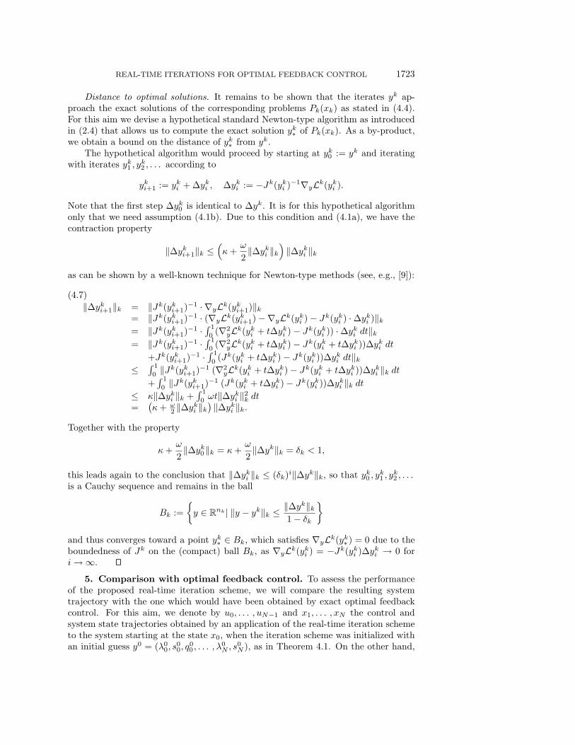
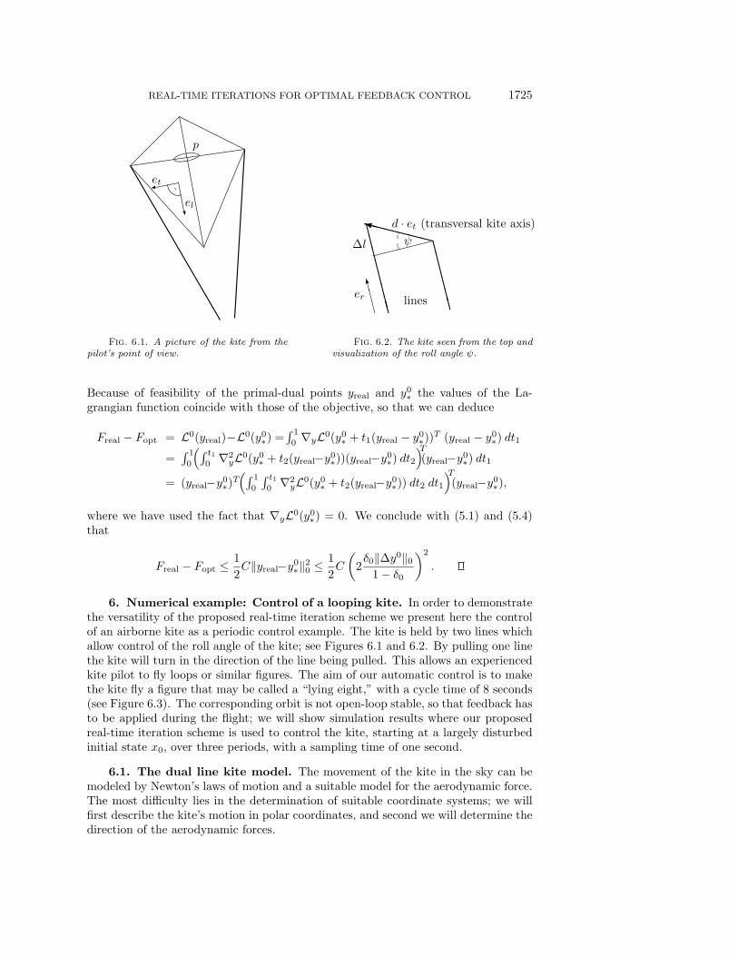
6. Numerical example: Control of a looping kite. In order to demonstratethe versatility of the proposed real-time iteration scheme we present here the controlof an airborne kite as a periodic control example. The kite is held by two lines whichallow control of the roll angle of the kite; see Figures 6.1 and 6.2. By pulling one linethe kite will turn in the direction of the line being pulled. This allows an experiencedkite pilot to fly loops or similar figures. The aim of our automatic control is to makethe kite fly a figure that may be called a “lying eight,” with a cycle time of 8 seconds(see Figure 6.3). The corresponding orbit is not open-loop stable, so that feedback hasto be applied during the flight; we will show simulation results where our proposedreal-time iteration scheme is used to control the kite, starting at a largely disturbedinitial state x0, over three periods, with a sampling time of one second.
6.1. The dual line kite model. The movement of the kite in the sky can bemodeled by Newton’s laws of motion and a suitable model for the aerodynamic force.The most difficulty lies in the determination of suitable coordinate systems; we willfirst describe the kite’s motion in polar coordinates, and second we will determine thedirection of the aerodynamic forces.

1726 M. DIEHL, H. G. BOCK, AND J. P. SCHLODER
6.1.1. Newton’s laws of motion in polar coordinates. The position p ∈ R3
of the kite can be modeled in three-dimensional Euclidean space, choosing the positionof the kite pilot as the origin, and the third component p3 to be the height of the kiteabove the ground. With m denoting the mass of the kite and F ∈ R
3 the total forceacting on the kite, Newton’s law of motion reads
p =d 2p
dt2=
F
m.
Let us introduce polar coordinates θ, φ, r:
p =
⎛⎝ p1
p2
p3
⎞⎠ =
⎛⎝ r sin(θ) cos(φ)
r sin(θ) sin(φ)r cos(θ)
⎞⎠ .
Note that the distance r between pilot and kite is usually constant during flight, and θis the angle that the lines form with the vertical. Let us introduce a local right-handedcoordinate system with the three basis vectors
eθ =
⎛⎝ cos(θ) cos(φ)
cos(θ) sin(φ)− sin(θ)
⎞⎠ , eφ =
⎛⎝− sin(φ)
cos(φ)0
⎞⎠ , and er =
⎛⎝ sin(θ) cos(φ)
sin(θ) sin(φ)cos(θ)
⎞⎠ .
Defining Fθ := F · eθ, Fφ := F · eφ, and Fr := F · er, we can write Newton’s laws ofmotion in the form
rθ − r sin(θ) cos(θ)φ2 + 2rθ =Fθ
m,
r sin(θ)φ + 2r cos(θ)φθ + 2 sin(θ)rφ =Fφ
m,
r − rθ2 − r sin2(θ)φ2 =Fr
m.(6.1)
If the length of the lines, denoted by r, is kept constant, all terms involving time deriva-tives of r will drop out. Furthermore, the last equation (6.1) will become redundant,as any acting force F ′
r in the radial direction will automatically be augmented by aconstraint force contribution Fc := Fr +mrθ2 +mr sin2(θ)φ2 so that (6.1) is satisfiedwith Fr := F ′
r −Fc. In this case we can regard only the components Fθ and Fφ whichare not changed by the constraint force. The equations of motion3 simplify to
θ =Fθ
rm+ sin(θ) cos(θ)φ2,(6.2)
φ =Fφ
rm sin(θ)− 2 cot(θ)φθ.(6.3)
In our model, the force F acting on the kite consists of three contributions, constraintforce −Fcer, gravitational force F gra, and aerodynamic force F aer. In Cartesian co-ordinates, F gra = (0, 0,−mg)T with g = 9.81 m s−2 being the earth’s gravitationalacceleration. In local coordinates we therefore have
Fθ = F graθ + F aer
θ = sin(θ)mg + F aerθ and Fφ = F aer
φ .
It remains to derive an expression for the aerodynamic force F aer.
3Note that the validity of these equations requires that Fc ≥ 0, as a line can only pull and notpush.

REAL-TIME ITERATIONS FOR OPTIMAL FEEDBACK CONTROL 1727
6.1.2. Kite orientation and the aerodynamic force. To model the aerody-namic force that is acting on the kite, we first assume that the kite’s trailing edgeis always pulled by the tail into the direction of the effective wind, as seen from thekite’s body-fixed frame. This assumption can be regarded as the limiting case of verylarge tail force. It crucially simplifies the model by allowing us to disregard angularmomentum and the moments acting on the kite. Under this assumption we are ableto determine the kite orientation as an explicit function of position and velocity only,as shown in the following.
By the large tail force assumption, the kite’s longitudinal axis is always in linewith the effective wind vector we := w − p, where w = (vw, 0, 0)T is the wind asseen from the earth system, and p is the kite velocity. If we introduce a unit vectorel pointing from the front toward the trailing edge of the kite (cf. Figure 6.1), wetherefore assume that
el =we
‖we‖.
The transversal axis of the kite can be described by a perpendicular unit vector etthat is pointing from the left to the right wing tip. Clearly, it is orthogonal to thelongitudinal axis, i.e.,
et · el =et · we
‖we‖= 0.(6.4)
The orientation of the transversal axis et against the lines’ axis (which is given bythe vector er) can be influenced by the length difference ∆l of the two lines. If thedistance between the two lines’ fixing points on the kite is d, then the vector from theleft to the right fixing point is det, and the projection of this vector onto the lines’axis should equal ∆l = det ·er, being positive if the left hand’s lines wingtip is fartheraway from the pilot; cf. Figure 6.2. Let us define the roll angle ψ to be
ψ = arcsin
(∆l
d
).
We will assume that we control this angle ψ directly. It determines the orientation ofet which has to satisfy
et · er =∆l
d= sin(ψ).(6.5)
A third requirement that et should satisfy is that
(el × et) · er =we × et‖we‖
· er > 0,(6.6)
which takes account of the fact that the kite is always in the same orientation withrespect to the lines.
How does one find a unit vector et that satisfies these requirements (6.4)–(6.6)?Using the projection wp
e of the effective wind vector we onto the tangent plane spannedby eθ and eφ,
wpe := eθ(eθ · we) + eφ(eφ · we) = we − er(er · we),
we can define the orthogonal unit vectors
ew :=wp
e
‖wpe‖
and eo := er × ew,

1728 M. DIEHL, H. G. BOCK, AND J. P. SCHLODER
so that (ew, eo, er) forms an orthogonal right-handed coordinate basis. Note thatin this basis the effective wind we has no component in the eo direction, as we =‖wp
e‖ew + (we · er)er. We will show that the definition
et := ew(− cos(ψ) sin(η)) + eo(cos(ψ) cos(η)) + er sin(ψ)(6.7)
with
η := arcsin
(we · er‖wp
e‖tan(ψ)
)
satisfies the requirements (6.4)–(6.6).4 Equation (6.4) can be verified by substitutionof the definition of η into
et · we = − cos(ψ) sin(η)‖wpe‖ + sin(ψ)(we · er) = 0.
Equation (6.5) is trivially satisfied, and (6.6) can be verified by calculation of
(we × et) · er = (we · ew) cos(ψ) cos(η) − (we · eo)(− cos(ψ) sin(η))= ‖wp
e‖ cos(ψ) cos(η)
(where we used the fact that we · eo = 0). For angles ψ and η in the range from−π/2 to π/2 this expression is always positive. The above considerations allow usto determine the orientation of the kite depending on the control ψ and the effectivewind we only. Note that the considerations would break down if the projection of theeffective wind wp
e would be equal to zero, if |ψ| ≥ π2 , or if∣∣∣∣we · er
‖wpe‖
tan(ψ)
∣∣∣∣ > 1.
The two vectors en := el × et and el are the directions of aerodynamic lift and drag,respectively. To compute the magnitudes FL and FD of lift and drag we assume thatthe lift and drag coefficients CL and CD are constant, so that we have
FL =1
2ρ‖we‖2ACL and FD =
1
2ρ‖we‖2ACD,
with ρ being the density of air and A being the characteristic area of the kite. Giventhe directions and magnitudes of lift and drag, we can compute F aer as their sum,yielding F aer = FLen + FDel, or, in the local coordinate system,
F aerθ = FL(en · eθ) + FD(el · eθ) and F aer
φ = FL(en · eφ) + FD(el · eφ).
The system parameters that have been chosen for the simulation model are listed inTable 6.1. Defining the system state ξ := (θ, φ, θ, φ)T and the control u := ψ, wecan summarize the four system equations, i.e., (6.2)–(6.3) and the trivial equations∂θ∂t = θ, ∂φ
∂t = φ, in the short form
ξ = f(ξ, u).
4It is interesting to note that the assignment of et can be made more transparent by consideringa rotation from the (ew, eo, er) tangential frame to the body frame (el, et, en), with en := el × et.Specifically, starting from (ew, eo, er), we rotate about the er-axis through the yaw angle −η andthen roll through the angle ψ about the el-axis. From this we find that et as the second basis vectorof the body frame is represented by (6.7) in the tangential frame (ew, eo, er).
REAL-TIME ITERATIONS FOR OPTIMAL FEEDBACK CONTROL 1729
Table 6.1
The kite parameters.
Name Symbol ValueLine length r 50 mKite mass m 1 kgWind velocity vw 6 m/sDensity of air ρ 1.2 kg/m3
Characteristic area A 0.5 m2
Lift coefficient CL 1.5Drag coefficient CD 0.29
60 40 20 0 -20 -40 -6090
80
70
60
50
40
30
θ [d
eg]
φ [deg]
1
2
3
4
5
6
7
0/8
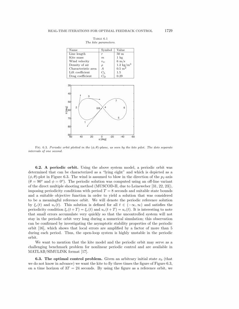
Fig. 6.3. Periodic orbit plotted in the (φ, θ)-plane, as seen by the kite pilot. The dots separateintervals of one second.
6.2. A periodic orbit. Using the above system model, a periodic orbit wasdetermined that can be characterized as a “lying eight” and which is depicted as a(φ, θ)-plot in Figure 6.3. The wind is assumed to blow in the direction of the p1-axis(θ = 90o and φ = 0o). The periodic solution was computed using an off-line variantof the direct multiple shooting method (MUSCOD-II, due to Leineweber [31, 22, 23]),imposing periodicity conditions with period T = 8 seconds and suitable state boundsand a suitable objective function in order to yield a solution that was consideredto be a meaningful reference orbit. We will denote the periodic reference solutionby ξr(t) and ur(t). This solution is defined for all t ∈ (−∞,∞) and satisfies theperiodicity condition ξr(t+T ) = ξr(t) and ur(t+T ) = ur(t). It is interesting to notethat small errors accumulate very quickly so that the uncontrolled system will notstay in the periodic orbit very long during a numerical simulation; this observationcan be confirmed by investigating the asymptotic stability properties of the periodicorbit [16], which shows that local errors are amplified by a factor of more than 5during each period. Thus, the open-loop system is highly unstable in the periodicorbit.
We want to mention that the kite model and the periodic orbit may serve as achallenging benchmark problem for nonlinear periodic control and are available inMATLAB/SIMULINK format [17].
6.3. The optimal control problem. Given an arbitrary initial state x0 (thatwe do not know in advance) we want the kite to fly three times the figure of Figure 6.3,on a time horizon of 3T = 24 seconds. By using the figure as a reference orbit, we

1730 M. DIEHL, H. G. BOCK, AND J. P. SCHLODER
formulate an optimal control problem which has the objective of bringing the systemclose to the reference orbit. For this aim we define a Lagrange term of least squarestype
L(ξ, u, t) :=1
2(ξ − ξr(t))
TQ(ξ − ξr(t)) +1
2(u− ur(t))
TR(u− ur(t))
with diagonal weighting matrices
Q := diag(0.4, 1, s2, s2)1
sand R := 1.0 · 10−2deg−2s−1.
Using these definitions, we formulate the following optimal control problem on thetime horizon of interest [0, 3T ]:
minu(·),ξ(·)
∫ 3T
0
L(ξ(t), u(t), t) dt(6.8)
subject to
ξ(t) = f(ξ(t), u(t)) ∀t ∈ [0, 3T ],
ξ(0) = x0.
6.4. Direct multiple shooting formulation. In order to reformulate theabove continuous optimal control problem into a discrete-time optimal controlproblem, we use the direct multiple shooting technique, originally due to Plittand Bock [35, 12]: We divide the time horizon into N = 24 invervals [ti, ti+1],each of one second length, and introduce a locally constant control representationq0, q1, . . . , qN−1, as well as artificial initial values s0, . . . , sN , as depicted in Figure 1.1.On each of these intervals we solve the following initial value problem:
ξi(t; si, qi) = f (ξi(t; si, qi), qi) , t ∈ [ti, ti+1],(6.9)
ξi(ti; si, qi) = si,
yielding a trajectory piece ξi(t; si, qi) for t ∈ [ti, ti+1]. This allows us to convenientlydefine a discrete-time system as in (1.2c) with transition function
fi(si, qi) := ξi(ti+1; si, qi).
Analogously, we define the objective contributions in (1.2a) by
Li(si, qi) :=
∫ ti+1
ti
L(ξi(t; si, qi), qi, t)dt.
The main difficulty of the direct multiple shooting method lies in the efficient solutionof the initial value problems (6.9) and in the sensitivity computation. For this aimwe use the advanced backward differentiation formula (BDF) code DAESOL (Bauer,Bock, and Schloder [3], Bauer [2]), which is especially suited for stiff problems, as theabove kite model. It uses the principle of internal numerical differentiation (IND) asintroduced by Bock [8].
Using the multiple shooting formulation, we have transformed the continuous-time optimization problem (6.8) into a nonlinear programming problem P0(x0) ofexactly the type (1.2).
REAL-TIME ITERATIONS FOR OPTIMAL FEEDBACK CONTROL 1731
80 60 40 20 0 20 40 60 8090
80
70
60
50
40
30
20
θ [d
eg]
φ [deg]80 60 40 20 0 - 0 - 0 - 0 - 0
90
80
70
60
50
40
30
20
θ [d
eg]
φ [deg]
x0
Fig. 6.4. Closed-loop trajectories resulting from the real-time iteration scheme for differentinitial values x0. The kite never crashes onto the ground (θ = 90 degrees).
6.4.1. Generation of the Gauss–Newton Hessian blocks. The efficientgeneration of a Gauss–Newton approximation for continuous least squares terms de-serves some attention: the Hessian approximations (2.6) are determined accordingto (
QHi MH
i
(MHi )T RH
i
):=
∫ ti+1
ti
(∂ξi(t; si, qi)
∂(si, qi)
)T
Q∂ξi(t; si, qi)
∂(si, qi)+
(0 00 R
)dt.
These integrals are efficiently computed during the sensitivity computation using aspecially adapted version of the integrator DAESOL [16, 25].
6.5. A real-time scenario. In the following real-time scenario we assume thatthe Newton-type optimizer is initialized with the reference trajectory itself, i.e., y0 :=(λ0
0, s00, q
00 , . . . , λ
0N , s0
N ), where λ0i := 0, and s0
i := ξr(ti) and q0i := 1
ti+1−ti
∫ ti+1
tiur(t)dt
are the corresponding values of the periodic reference solution. This y0 is (nearly)identical to the solution of the problem P0(ξr(t0)). At the time t0 = 0, when the actualvalue of x0 is known, we start the iterations as described in section 3.1 by solving thefirst prepared linear system ∆y0 = −J0(y0)−1∇yL0(y0) (step 2) and give the firstcontrol u0 := q0
0 +∆q00 immediately to the system. Then we shrink the problem (step
3) and prepare the iteration for the following one (step 1). As we assume no furtherdisturbances, the new initial value is x1 = f0(x0, u0) = ξ0(t1;x0, u0) resulting fromthe (continuous) system dynamics. This cycle is repeated until the N = 24 intervalsare over.
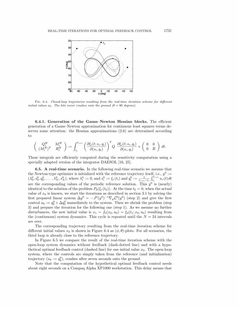
The corresponding trajectory resulting from the real-time iteration scheme fordifferent initial values x0 is shown in Figure 6.4 as (φ, θ)-plots. For all scenarios, thethird loop is already close to the reference trajectory.
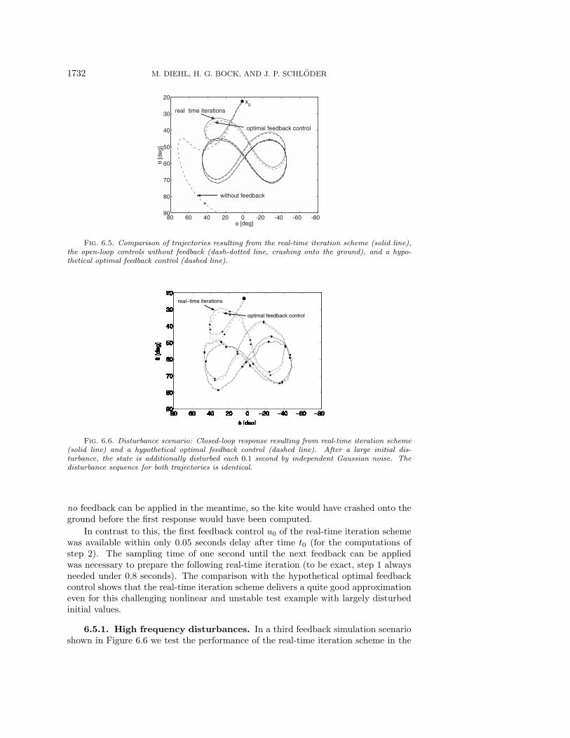
In Figure 6.5 we compare the result of the real-time iteration scheme with theopen-loop system dynamics without feedback (dash-dotted line) and with a hypo-thetical optimal feedback control (dashed line) for one initial value x0. The open-loopsystem, where the controls are simply taken from the reference (and initialization)trajectory (uk := q0
k), crashes after seven seconds onto the ground.Note that the computation of the hypothetical optimal feedback control needs
about eight seconds on a Compaq Alpha XP1000 workstation. This delay means that
1732 M. DIEHL, H. G. BOCK, AND J. P. SCHLODER
80 60 40 20 0 -20 -40 -60 -8090
80
70
60
50
40
30
20
θ [d
eg]
φ [deg]
without feedback
real time iterations
optimal feedback control
x0
Fig. 6.5. Comparison of trajectories resulting from the real-time iteration scheme (solid line),the open-loop controls without feedback (dash-dotted line, crashing onto the ground), and a hypo-thetical optimal feedback control (dashed line).
−80−60−40−20020406080
20
30
40
50
60
70
80
90
θ [d
eg]
φ [deg]
−80−60−40−20020406080
20
30
40
50
60
70
80
90
θ [d
eg]
φ [deg]
−80−60−40−20020406080
20
30
40
50
60
70
80
90
θ [d
eg]
φ [deg]
−80−60−40−20020406080
20
30
40
50
60
70
80
90
θ [d
eg]
φ [deg]
−80−60−40−20020406080
20
30
40
50
60
70
80
90
θ [d
eg]
φ [deg]
−80−60−40−20020406080
20
30
40
50
60
70
80
90
θ [d
eg]
φ [deg]
−80−60−40−20020406080
20
30
40
50
60
70
80
90
θ [d
eg]
φ [deg]
−80−60−40−20020406080
20
30
40
50
60
70
80
90
θ [d
eg]
φ [deg]
−80−60−40−20020406080
20
30
40
50
60
70
80
90
θ [d
eg]
φ [deg]
−80−60−40−20020406080
20
30
40
50
60
70
80
90
θ [d
eg]
φ [deg]
−80−60−40−20020406080
20
30
40
50
60
70
80
90
θ [d
eg]
φ [deg]
−80−60−40−20020406080
20
30
40
50
60
70
80
90
θ [d
eg]
φ [deg]
−80−60−40−20020406080
20
30
40
50
60
70
80
90
θ [d
eg]
φ [deg]
−80−60−40−20020406080
20
30
40
50
60
70
80
90
θ [d
eg]
φ [deg]
−80−60−40−20020406080
20
30
40
50
60
70
80
90
θ [d
eg]
φ [deg]
−80−60−40−20020406080
20
30
40
50
60
70
80
90
θ [d
eg]
φ [deg]
−80−60−40−20020406080
20
30
40
50
60
70
80
90
θ [d
eg]
φ [deg]
−80−60−40−20020406080
20
30
40
50
60
70
80
90
θ [d
eg]
φ [deg]
−80−60−40−20020406080
20
30
40
50
60
70
80
90
θ [d
eg]
φ [deg]
−80−60−40−20020406080
20
30
40
50
60
70
80
90
θ [d
eg]
φ [deg]
−80−60−40−20020406080
20
30
40
50
60
70
80
90
θ [d
eg]
φ [deg]
−80−60−40−20020406080
20
30
40
50
60
70
80
90
θ [d
eg]
φ [deg]
−80−60−40−20020406080
20
30
40
50
60
70
80
90
θ [d
eg]
φ [deg]
−80−60−40−20020406080
20
30
40
50
60
70
80
90
θ [d
eg]
φ [deg]
−80−60−40−20020406080
20
30
40
50
60
70
80
90
θ [d
eg]
φ [deg]
−80−60−40−20020406080
20
30
40
50
60
70
80
90
θ [d
eg]
φ [deg]
−80−60−40−20020406080
20
30
40
50
60
70
80
90
θ [d
eg]
φ [deg]
−80−60−40−20020406080
20
30
40
50
60
70
80
90
θ [d
eg]
φ [deg]
−80−60−40−20020406080
20
30
40
50
60
70
80
90
θ [d
eg]
φ [deg]
−80−60−40−20020406080
20
30
40
50
60
70
80
90
θ [d
eg]
φ [deg]
−80−60−40−20020406080
20
30
40
50
60
70
80
90
θ [d
eg]
φ [deg]
−80−60−40−20020406080
20
30
40
50
60
70
80
90
θ [d
eg]
φ [deg]
−80−60−40−20020406080
20
30
40
50
60
70
80
90
θ [d
eg]
φ [deg]
−80−60−40−20020406080
20
30
40
50
60
70
80
90
θ [d
eg]
φ [deg]
−80−60−40−20020406080
20
30
40
50
60
70
80
90
θ [d
eg]
φ [deg]
−80−60−40−20020406080
20
30
40
50
60
70
80
90
θ [d
eg]
φ [deg]
−80−60−40−20020406080
20
30
40
50
60
70
80
90
θ [d
eg]
φ [deg]
−80−60−40−20020406080
20
30
40
50
60
70
80
90
θ [d
eg]
φ [deg]
−80−60−40−20020406080
20
30
40
50
60
70
80
90
θ [d
eg]
φ [deg]
−80−60−40−20020406080
20
30
40
50
60
70
80
90
θ [d
eg]
φ [deg]
−80−60−40−20020406080
20
30
40
50
60
70
80
90
θ [d
eg]
φ [deg]
−80−60−40−20020406080
20
30
40
50
60
70
80
90
θ [d
eg]
φ [deg]
−80−60−40−20020406080
20
30
40
50
60
70
80
90
θ [d
eg]
φ [deg]
−80−60−40−20020406080
20
30
40
50
60
70
80
90
θ [d
eg]
φ [deg]
−80−60−40−20020406080
20
30
40
50
60
70
80
90
θ [d
eg]
φ [deg]
−80−60−40−20020406080
20
30
40
50
60
70
80
90
θ [d
eg]
φ [deg]
−80−60−40−20020406080
20
30
40
50
60
70
80
90
θ [d
eg]
φ [deg]
−80−60−40−20020406080
20
30
40
50
60
70
80
90
θ [d
eg]
φ [deg]
−80−60−40−20020406080
20
30
40
50
60
70
80
90
θ [d
eg]
φ [deg]
−80−60−40−20020406080
20
30
40
50
60
70
80
90
θ [d
eg]
φ [deg]
−80−60−40−20020406080
20
30
40
50
60
70
80
90
θ [d
eg]
φ [deg]
−80−60−40−20020406080
20
30
40
50
60
70
80
90
θ [d
eg]
φ [deg]
−80−60−40−20020406080
20
30
40
50
60
70
80
90
θ [d
eg]
φ [deg]
−80−60−40−20020406080
20
30
40
50
60
70
80
90
θ [d
eg]
φ [deg]
−80−60−40−20020406080
20
30
40
50
60
70
80
90
θ [d
eg]
φ [deg]
−80−60−40−20020406080
20
30
40
50
60
70
80
90
θ [d
eg]
φ [deg]
−80−60−40−20020406080
20
30
40
50
60
70
80
90
θ [d
eg]
φ [deg]
−80−60−40−20020406080
20
30
40
50
60
70
80
90
θ [d
eg]
φ [deg]
−80−60−40−20020406080
20
30
40
50
60
70
80
90
θ [d
eg]
φ [deg]
−80−60−40−20020406080
20
30
40
50
60
70
80
90
θ [d
eg]
φ [deg]
−80−60−40−20020406080
20
30
40
50
60
70
80
90
θ [d
eg]
φ [deg]
−80−60−40−20020406080
20
30
40
50
60
70
80
90
θ [d
eg]
φ [deg]
−80−60−40−20020406080
20
30
40
50
60
70
80
90
θ [d
eg]
φ [deg]
−80−60−40−20020406080
20
30
40
50
60
70
80
90
θ [d
eg]
φ [deg]
−80−60−40−20020406080
20
30
40
50
60
70
80
90
θ [d
eg]
φ [deg]
−80−60−40−20020406080
20
30
40
50
60
70
80
90
θ [d
eg]
φ [deg]
−80−60−40−20020406080
20
30
40
50
60
70
80
90
θ [d
eg]
φ [deg]
−80−60−40−20020406080
20
30
40
50
60
70
80
90
θ [d
eg]
φ [deg]
−80−60−40−20020406080
20
30
40
50
60
70
80
90
θ [d
eg]
φ [deg]
−80−60−40−20020406080
20
30
40
50
60
70
80
90
θ [d
eg]
φ [deg]
−80−60−40−20020406080
20
30
40
50
60
70
80
90
θ [d
eg]
φ [deg]
−80−60−40−20020406080
20
30
40
50
60
70
80
90
θ [d
eg]
φ [deg]
−80−60−40−20020406080
20
30
40
50
60
70
80
90
θ [d
eg]
φ [deg]
−80−60−40−20020406080
20
30
40
50
60
70
80
90
θ [d
eg]
φ [deg]
−80−60−40−20020406080
20
30
40
50
60
70
80
90
θ [d
eg]
φ [deg]
−80−60−40−20020406080
20
30
40
50
60
70
80
90
θ [d
eg]
φ [deg]
−80−60−40−20020406080
20
30
40
50
60
70
80
90
θ [d
eg]
φ [deg]
−80−60−40−20020406080
20
30
40
50
60
70
80
90
θ [d
eg]
φ [deg]
−80−60−40−20020406080
20
30
40
50
60
70
80
90
θ [d
eg]
φ [deg]
−80−60−40−20020406080
20
30
40
50
60
70
80
90
θ [d
eg]
φ [deg]
−80−60−40−20020406080
20
30
40
50
60
70
80
90
θ [d
eg]
φ [deg]
−80−60−40−20020406080
20
30
40
50
60
70
80
90
θ [d
eg]
φ [deg]
−80−60−40−20020406080
20
30
40
50
60
70
80
90
θ [d
eg]
φ [deg]
−80−60−40−20020406080
20
30
40
50
60
70
80
90
θ [d
eg]
φ [deg]
−80−60−40−20020406080
20
30
40
50
60
70
80
90
θ [d
eg]
φ [deg]
−80−60−40−20020406080
20
30
40
50
60
70
80
90
θ [d
eg]
φ [deg]
−80−60−40−20020406080
20
30
40
50
60
70
80
90
θ [d
eg]
φ [deg]
−80−60−40−20020406080
20
30
40
50
60
70
80
90
θ [d
eg]
φ [deg]
−80−60−40−20020406080
20
30
40
50
60
70
80
90
θ [d
eg]
φ [deg]
−80−60−40−20020406080
20
30
40
50
60
70
80
90
θ [d
eg]
φ [deg]
−80−60−40−20020406080
20
30
40
50
60
70
80
90
θ [d
eg]
φ [deg]
−80−60−40−20020406080
20
30
40
50
60
70
80
90
θ [d
eg]
φ [deg]
−80−60−40−20020406080
20
30
40
50
60
70
80
90
θ [d
eg]
φ [deg]
−80−60−40−20020406080
20
30
40
50
60
70
80
90
θ [d
eg]
φ [deg]
−80−60−40−20020406080
20
30
40
50
60
70
80
90
θ [d
eg]
φ [deg]
−80−60−40−20020406080
20
30
40
50
60
70
80
90
θ [d
eg]
φ [deg]
−80−60−40−20020406080
20
30
40
50
60
70
80
90
θ [d
eg]
φ [deg]
−80−60−40−20020406080
20
30
40
50
60
70
80
90
θ [d
eg]
φ [deg]
−80−60−40−20020406080
20
30
40
50
60
70
80
90
θ [d
eg]
φ [deg]
−80−60−40−20020406080
20
30
40
50
60
70
80
90
θ [d
eg]
φ [deg]
−80−60−40−20020406080
20
30
40
50
60
70
80
90
θ [d
eg]
φ [deg]
−80−60−40−20020406080
20
30
40
50
60
70
80
90
θ [d
eg]
φ [deg]
−80−60−40−20020406080
20
30
40
50
60
70
80
90
θ [d
eg]
φ [deg]
−80−60−40−20020406080
20
30
40
50
60
70
80
90
θ [d
eg]
φ [deg]
−80−60−40−20020406080
20
30
40
50
60
70
80
90
θ [d
eg]
φ [deg]
−80−60−40−20020406080
20
30
40
50
60
70
80
90
θ [d
eg]
φ [deg]
−80−60−40−20020406080
20
30
40
50
60
70
80
90
θ [d
eg]
φ [deg]
−80−60−40−20020406080
20
30
40
50
60
70
80
90
θ [d
eg]
φ [deg]
−80−60−40−20020406080
20
30
40
50
60
70
80
90
θ [d
eg]
φ [deg]
−80−60−40−20020406080
20
30
40
50
60
70
80
90
θ [d
eg]
φ [deg]
−80−60−40−20020406080
20
30
40
50
60
70
80
90
θ [d
eg]
φ [deg]
−80−60−40−20020406080
20
30
40
50
60
70
80
90
θ [d
eg]
φ [deg]
−80−60−40−20020406080
20
30
40
50
60
70
80
90
θ [d
eg]
φ [deg]
−80−60−40−20020406080
20
30
40
50
60
70
80
90
θ [d
eg]
φ [deg]
−80−60−40−20020406080
20
30
40
50
60
70
80
90
θ [d
eg]
φ [deg]
−80−60−40−20020406080
20
30
40
50
60
70
80
90
θ [d
eg]
φ [deg]
−80−60−40−20020406080
20
30
40
50
60
70
80
90
θ [d
eg]
φ [deg]
−80−60−40−20020406080
20
30
40
50
60
70
80
90
θ [d
eg]
φ [deg]
−80−60−40−20020406080
20
30
40
50
60
70
80
90
θ [d
eg]
φ [deg]
−80−60−40−20020406080
20
30
40
50
60
70
80
90
θ [d
eg]
φ [deg]
−80−60−40−20020406080
20
30
40
50
60
70
80
90
θ [d
eg]
φ [deg]
−80−60−40−20020406080
20
30
40
50
60
70
80
90
θ [d
eg]
φ [deg]
−80−60−40−20020406080
20
30
40
50
60
70
80
90
θ [d
eg]
φ [deg]
−80−60−40−20020406080
20
30
40
50
60
70
80
90
θ [d
eg]
φ [deg]
−80−60−40−20020406080
20
30
40
50
60
70
80
90
θ [d
eg]
φ [deg]
−80−60−40−20020406080
20
30
40
50
60
70
80
90
θ [d
eg]
φ [deg]
−80−60−40−20020406080
20
30
40
50
60
70
80
90
θ [d
eg]
φ [deg]
−80−60−40−20020406080
20
30
40
50
60
70
80
90
θ [d
eg]
φ [deg]
−80−60−40−20020406080
20
30
40
50
60
70
80
90
θ [d
eg]
φ [deg]
−80−60−40−20020406080
20
30
40
50
60
70
80
90
θ [d
eg]
φ [deg]
−80−60−40−20020406080
20
30
40
50
60
70
80
90
θ [d
eg]
φ [deg]
−80−60−40−20020406080
20
30
40
50
60
70
80
90
θ [d
eg]
φ [deg]
−80−60−40−20020406080
20
30
40
50
60
70
80
90
θ [d
eg]
φ [deg]
−80−60−40−20020406080
20
30
40
50
60
70
80
90
θ [d
eg]
φ [deg]
−80−60−40−20020406080
20
30
40
50
60
70
80
90
θ [d
eg]
φ [deg]
−80−60−40−20020406080
20
30
40
50
60
70
80
90
θ [d
eg]
φ [deg]
−80−60−40−20020406080
20
30
40
50
60
70
80
90
θ [d
eg]
φ [deg]
−80−60−40−20020406080
20
30
40
50
60
70
80
90
θ [d
eg]
φ [deg]
−80−60−40−20020406080
20
30
40
50
60
70
80
90
θ [d
eg]
φ [deg]
−80−60−40−20020406080
20
30
40
50
60
70
80
90
θ [d
eg]
φ [deg]
−80−60−40−20020406080
20
30
40
50
60
70
80
90
θ [d
eg]
φ [deg]
−80−60−40−20020406080
20
30
40
50
60
70
80
90
θ [d
eg]
φ [deg]
−80−60−40−20020406080
20
30
40
50
60
70
80
90
θ [d
eg]
φ [deg]
−80−60−40−20020406080
20
30
40
50
60
70
80
90
θ [d
eg]
φ [deg]
−80−60−40−20020406080
20
30
40
50
60
70
80
90
θ [d
eg]
φ [deg]
−80−60−40−20020406080
20
30
40
50
60
70
80
90
θ [d
eg]
φ [deg]
−80−60−40−20020406080
20
30
40
50
60
70
80
90
θ [d
eg]
φ [deg]
−80−60−40−20020406080
20
30
40
50
60
70
80
90
θ [d
eg]
φ [deg]
−80−60−40−20020406080
20
30
40
50
60
70
80
90
θ [d
eg]
φ [deg]
−80−60−40−20020406080
20
30
40
50
60
70
80
90
θ [d
eg]
φ [deg]
−80−60−40−20020406080
20
30
40
50
60
70
80
90
θ [d
eg]
φ [deg]
−80−60−40−20020406080
20
30
40
50
60
70
80
90
θ [d
eg]
φ [deg]
−80−60−40−20020406080
20
30
40
50
60
70
80
90
θ [d
eg]
φ [deg]
−80−60−40−20020406080
20
30
40
50
60
70
80
90
θ [d
eg]
φ [deg]
−80−60−40−20020406080
20
30
40
50
60
70
80
90
θ [d
eg]
φ [deg]
−80−60−40−20020406080
20
30
40
50
60
70
80
90
θ [d
eg]
φ [deg]
−80−60−40−20020406080
20
30
40
50
60
70
80
90
θ [d
eg]
φ [deg]
−80−60−40−20020406080
20
30
40
50
60
70
80
90
θ [d
eg]
φ [deg]
−80−60−40−20020406080
20
30
40
50
60
70
80
90
θ [d
eg]
φ [deg]
−80−60−40−20020406080
20
30
40
50
60
70
80
90
θ [d
eg]
φ [deg]
−80−60−40−20020406080
20
30
40
50
60
70
80
90
θ [d
eg]
φ [deg]
−80−60−40−20020406080
20
30
40
50
60
70
80
90
θ [d
eg]
φ [deg]
−80−60−40−20020406080
20
30
40
50
60
70
80
90
θ [d
eg]
φ [deg]
−80−60−40−20020406080
20
30
40
50
60
70
80
90
θ [d
eg]
φ [deg]
−80−60−40−20020406080
20
30
40
50
60
70
80
90
θ [d
eg]
φ [deg]
−80−60−40−20020406080
20
30
40
50
60
70
80
90
θ [d
eg]
φ [deg]
−80−60−40−20020406080
20
30
40
50
60
70
80
90
θ [d
eg]
φ [deg]
−80−60−40−20020406080
20
30
40
50
60
70
80
90
θ [d
eg]
φ [deg]
−80−60−40−20020406080
20
30
40
50
60
70
80
90
θ [d
eg]
φ [deg]
−80−60−40−20020406080
20
30
40
50
60
70
80
90
θ [d
eg]
φ [deg]
−80−60−40−20020406080
20
30
40
50
60
70
80
90
θ [d
eg]
φ [deg]
−80−60−40−20020406080
20
30
40
50
60
70
80
90
θ [d
eg]
φ [deg]
−80−60−40−20020406080
20
30
40
50
60
70
80
90
θ [d
eg]
φ [deg]
−80−60−40−20020406080
20
30
40
50
60
70
80
90
θ [d
eg]
φ [deg]
−80−60−40−20020406080
20
30
40
50
60
70
80
90
θ [d
eg]
φ [deg]
−80−60−40−20020406080
20
30
40
50
60
70
80
90
θ [d
eg]
φ [deg]
−80−60−40−20020406080
20
30
40
50
60
70
80
90
θ [d
eg]
φ [deg]
−80−60−40−20020406080
20
30
40
50
60
70
80
90
θ [d
eg]
φ [deg]
−80−60−40−20020406080
20
30
40
50
60
70
80
90
θ [d
eg]
φ [deg]
−80−60−40−20020406080
20
30
40
50
60
70
80
90
θ [d
eg]
φ [deg]
−80−60−40−20020406080
20
30
40
50
60
70
80
90
θ [d
eg]
φ [deg]
−80−60−40−20020406080
20
30
40
50
60
70
80
90
θ [d
eg]
φ [deg]
−80−60−40−20020406080
20
30
40
50
60
70
80
90
θ [d
eg]
φ [deg]
−80−60−40−20020406080
20
30
40
50
60
70
80
90
real−time iterations
optimal feedback control
Fig. 6.6. Disturbance scenario: Closed-loop response resulting from real-time iteration scheme(solid line) and a hypothetical optimal feedback control (dashed line). After a large initial dis-turbance, the state is additionally disturbed each 0.1 second by independent Gaussian noise. Thedisturbance sequence for both trajectories is identical.
no feedback can be applied in the meantime, so the kite would have crashed onto theground before the first response would have been computed.
In contrast to this, the first feedback control u0 of the real-time iteration schemewas available within only 0.05 seconds delay after time t0 (for the computations ofstep 2). The sampling time of one second until the next feedback can be appliedwas necessary to prepare the following real-time iteration (to be exact, step 1 alwaysneeded under 0.8 seconds). The comparison with the hypothetical optimal feedbackcontrol shows that the real-time iteration scheme delivers a quite good approximationeven for this challenging nonlinear and unstable test example with largely disturbedinitial values.
6.5.1. High frequency disturbances. In a third feedback simulation scenarioshown in Figure 6.6 we test the performance of the real-time iteration scheme in the

REAL-TIME ITERATIONS FOR OPTIMAL FEEDBACK CONTROL 1733
presence of random disturbances with a frequency higher than the sampling time: eachtenth of a second the state (θ, φ, θ, φ) is randomly disturbed by independent Gaussiannoise of standard deviation 0.01 · (1, 1, s−1, s−1). Because feedback is provided onlyonce a second, the kite flies open-loop during one second before feedback can be pro-vided to the accumulated result of the disturbances. The initial state was much morestrongly disturbed, in the same way as in the scenario of Figure 6.5. Despite thesecombined disturbances the scheme is able to lead the kite efficiently into the referenceorbit. Again, it compares well with optimal feedback control. Note, however, thatthe results of Theorems 4.1 and 5.1 are not directly applicable to this third scenarioas these theorems assume undisturbed system behavior after one initial disturbance.
For feedback control simulations of the kite using a moving horizon frameworkincluding also state constraints, we refer to [16, 24].
7. Conclusions. We have presented a recently developed Newton-type methodfor the real-time optimization of nonlinear processes and have given a new contractiv-ity result and a bound on the loss of optimality when compared to optimal feedbackcontrol. In a numerical case study, the real-time control of an airborne kite, we havedemonstrated the practical applicability of the method for a challenging nonlinearcontrol example.
The “real-time iteration” scheme is based on the direct multiple shooting method,which offers several advantages in the context of real-time optimal control, amongthem the ability to efficiently initialize subsequent optimization problems, to treathighly nonlinear and unstable systems, and to deal efficiently with path constraints.The most important feature of the real-time iteration scheme is a dovetailing of thesolution iterations with the process development which allows us to reduce samplingtimes to a minimum but maintains all advantages of a fully nonlinear treatment of theoptimization problems. A separation of the computations in each real-time iterationinto a preparation phase and a feedback response phase can be realized. The feedbackphase is typically orders of magnitude shorter than the preparation phase and allowsus to obtain an immediate feedback that takes all linearized constraints into account.
The contractivity of the scheme is proven under mild conditions that are nearlyidentical to the sufficient conditions for convergence of off-line Newton-type methods.Iterates on different horizon lengths have to be compared. The result is that the real-time iterates, after an initial disturbance, geometrically approach the exact optimalsolutions during the runtime of the process. When the resulting closed-loop trajectoryis compared to optimal feedback control, a bound on the loss of optimality has beenestablished, which is of fourth order in the initial disturbance if an exact Newton–Raphson method is used.
A newly developed kite model is presented. The control aim is, starting from anarbitrary initial state, to steer the kite into a periodic orbit, a “lying eight” with aperiod duration of eight seconds. We consider a time horizon of 24 seconds. The initialstate is only known at the moment that the first control needs already to be applied;the real-time iteration scheme delivers linearized feedback nearly without delay andprovides a newly linearized feedback after each sampling time of one second, leading toa fully nonlinear optimization, and is always prepared to react to further disturbances.The scheme shows an excellent closed-loop performance for this highly nonlinear andunstable system and compares well to a hypothetical exact optimal feedback control.
The real-time iteration scheme has also been applied for NMPC of a real pilotplant distillation column described by a stiff DAE model with over 200 system states,allowing feedback sampling times of only 20 seconds [21].
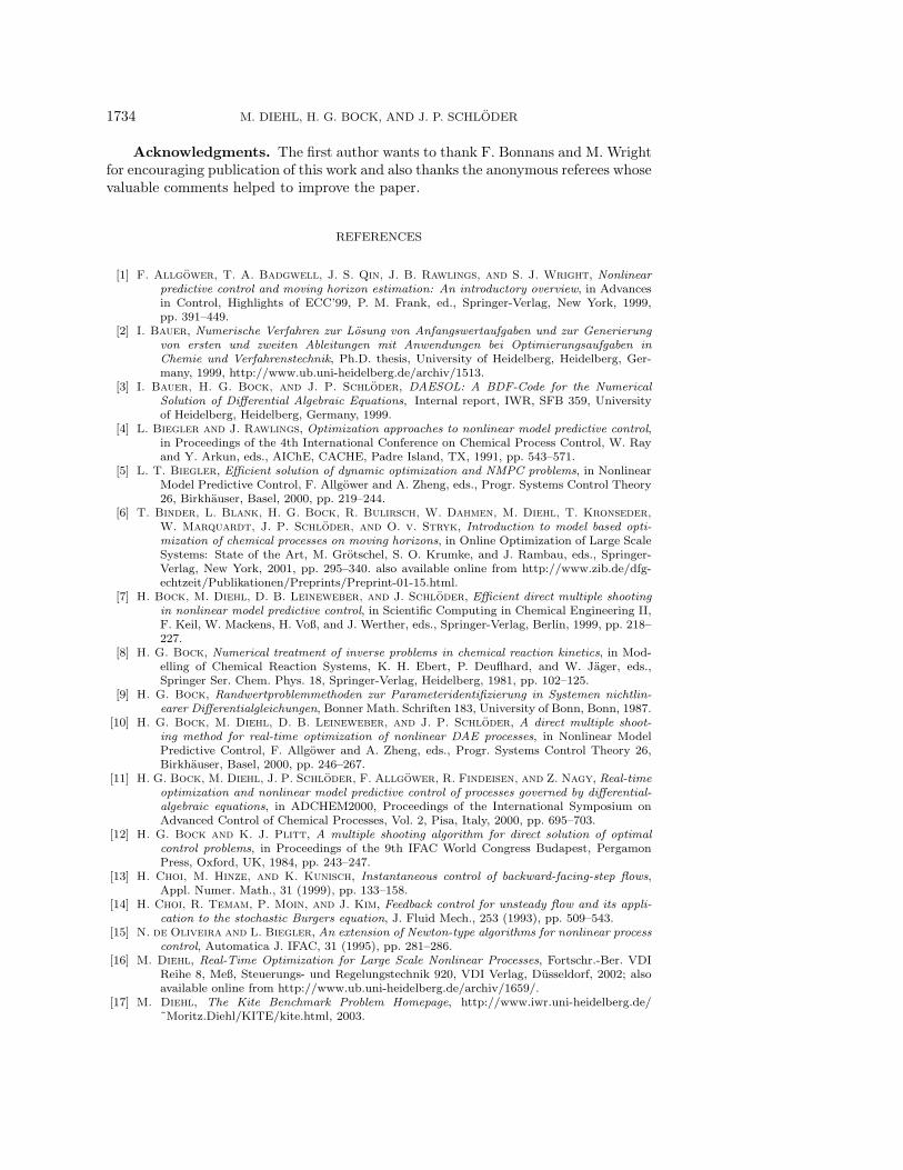
1734 M. DIEHL, H. G. BOCK, AND J. P. SCHLODER
Acknowledgments. The first author wants to thank F. Bonnans and M. Wrightfor encouraging publication of this work and also thanks the anonymous referees whosevaluable comments helped to improve the paper.
REFERENCES
[1] F. Allgower, T. A. Badgwell, J. S. Qin, J. B. Rawlings, and S. J. Wright, Nonlinearpredictive control and moving horizon estimation: An introductory overview, in Advancesin Control, Highlights of ECC’99, P. M. Frank, ed., Springer-Verlag, New York, 1999,pp. 391–449.
[2] I. Bauer, Numerische Verfahren zur Losung von Anfangswertaufgaben und zur Generierungvon ersten und zweiten Ableitungen mit Anwendungen bei Optimierungsaufgaben inChemie und Verfahrenstechnik, Ph.D. thesis, University of Heidelberg, Heidelberg, Ger-many, 1999, http://www.ub.uni-heidelberg.de/archiv/1513.
[3] I. Bauer, H. G. Bock, and J. P. Schloder, DAESOL: A BDF-Code for the NumericalSolution of Differential Algebraic Equations, Internal report, IWR, SFB 359, Universityof Heidelberg, Heidelberg, Germany, 1999.
[4] L. Biegler and J. Rawlings, Optimization approaches to nonlinear model predictive control,in Proceedings of the 4th International Conference on Chemical Process Control, W. Rayand Y. Arkun, eds., AIChE, CACHE, Padre Island, TX, 1991, pp. 543–571.
[5] L. T. Biegler, Efficient solution of dynamic optimization and NMPC problems, in NonlinearModel Predictive Control, F. Allgower and A. Zheng, eds., Progr. Systems Control Theory26, Birkhauser, Basel, 2000, pp. 219–244.
[6] T. Binder, L. Blank, H. G. Bock, R. Bulirsch, W. Dahmen, M. Diehl, T. Kronseder,
W. Marquardt, J. P. Schloder, and O. v. Stryk, Introduction to model based opti-mization of chemical processes on moving horizons, in Online Optimization of Large ScaleSystems: State of the Art, M. Grotschel, S. O. Krumke, and J. Rambau, eds., Springer-Verlag, New York, 2001, pp. 295–340. also available online from http://www.zib.de/dfg-echtzeit/Publikationen/Preprints/Preprint-01-15.html.
[7] H. Bock, M. Diehl, D. B. Leineweber, and J. Schloder, Efficient direct multiple shootingin nonlinear model predictive control, in Scientific Computing in Chemical Engineering II,F. Keil, W. Mackens, H. Voß, and J. Werther, eds., Springer-Verlag, Berlin, 1999, pp. 218–227.
[8] H. G. Bock, Numerical treatment of inverse problems in chemical reaction kinetics, in Mod-elling of Chemical Reaction Systems, K. H. Ebert, P. Deuflhard, and W. Jager, eds.,Springer Ser. Chem. Phys. 18, Springer-Verlag, Heidelberg, 1981, pp. 102–125.
[9] H. G. Bock, Randwertproblemmethoden zur Parameteridentifizierung in Systemen nichtlin-earer Differentialgleichungen, Bonner Math. Schriften 183, University of Bonn, Bonn, 1987.
[10] H. G. Bock, M. Diehl, D. B. Leineweber, and J. P. Schloder, A direct multiple shoot-ing method for real-time optimization of nonlinear DAE processes, in Nonlinear ModelPredictive Control, F. Allgower and A. Zheng, eds., Progr. Systems Control Theory 26,Birkhauser, Basel, 2000, pp. 246–267.
[11] H. G. Bock, M. Diehl, J. P. Schloder, F. Allgower, R. Findeisen, and Z. Nagy, Real-timeoptimization and nonlinear model predictive control of processes governed by differential-algebraic equations, in ADCHEM2000, Proceedings of the International Symposium onAdvanced Control of Chemical Processes, Vol. 2, Pisa, Italy, 2000, pp. 695–703.
[12] H. G. Bock and K. J. Plitt, A multiple shooting algorithm for direct solution of optimalcontrol problems, in Proceedings of the 9th IFAC World Congress Budapest, PergamonPress, Oxford, UK, 1984, pp. 243–247.
[13] H. Choi, M. Hinze, and K. Kunisch, Instantaneous control of backward-facing-step flows,Appl. Numer. Math., 31 (1999), pp. 133–158.
[14] H. Choi, R. Temam, P. Moin, and J. Kim, Feedback control for unsteady flow and its appli-cation to the stochastic Burgers equation, J. Fluid Mech., 253 (1993), pp. 509–543.
[15] N. de Oliveira and L. Biegler, An extension of Newton-type algorithms for nonlinear processcontrol, Automatica J. IFAC, 31 (1995), pp. 281–286.
[16] M. Diehl, Real-Time Optimization for Large Scale Nonlinear Processes, Fortschr.-Ber. VDIReihe 8, Meß, Steuerungs- und Regelungstechnik 920, VDI Verlag, Dusseldorf, 2002; alsoavailable online from http://www.ub.uni-heidelberg.de/archiv/1659/.
[17] M. Diehl, The Kite Benchmark Problem Homepage, http://www.iwr.uni-heidelberg.de/˜Moritz.Diehl/KITE/kite.html, 2003.
REAL-TIME ITERATIONS FOR OPTIMAL FEEDBACK CONTROL 1735
[18] M. Diehl, H. G. Bock, and J. P. Schloder, Newton-type methods for the approximatesolution of nonlinear programming problems in real time, in High Performance Algorithmsand Software for Nonlinear Optimization, G. D. Pillo and A. Murli, eds., Kluwer AcademicPublishers B.V., Dordrecht, The Netherlands, 2002, pp. 177–200.
[19] M. Diehl, H. G. Bock, J. P. Schloder, R. Findeisen, Z. Nagy, and F. Allgower, Real-timeoptimization and nonlinear model predictive control of processes governed by differential-algebraic equations, J. Proc. Contr., 12 (2002), pp. 577–585.
[20] M. Diehl, R. Findeisen, S. Schwarzkopf, I. Uslu, F. Allgower, H. G. Bock, E. D. Gilles,
and J. P. Schloder, An efficient algorithm for nonlinear model predictive control of large-scale systems. Part I: Description of the method, Automatisierungstechnik, 50 (2002), pp.557–567.
[21] M. Diehl, R. Findeisen, S. Schwarzkopf, I. Uslu, F. Allgower, H. G. Bock, E. D. Gilles,
and J. P. Schloder, An efficient algorithm for nonlinear model predictive control of large-scale systems. Part II: Application to a distillation column, Automatisierungstechnik, 51(2003), pp. 22–29.
[22] D. B. Leineweber, I. Bauer, H. G. Bock, and J. P. Schloder, An effficient multiple shootingbased reduced SQP strategy for large-scale dyamic process optimization. Part I: Theoreticalaspects, Comp. Chem. Engrg., 27 (2003), pp. 157–166.
[23] D. B. Leineweber, A. Schafer, H. G. Bock, and J. P. Schloder, An effficient multipleshooting based reduced SQP strategy for large-scale dyamic process optimization. Part II:Software aspects and applications, Comp. Chem. Engrg., 27 (2003), pp. 167–174.
[24] M. Diehl, L. Magni, and G. De Nicolao, Online NMPC of unstable periodic systems usingapproximate infinite horizon closed loop costing, Annual Reviews in Control, 28 (2004),pp. 37–45.
[25] M. Diehl, I. Uslu, R. Findeisen, S. Schwarzkopf, F. Allgower, H. G. Bock, T. Burner,
E. D. Gilles, A. Kienle, J. P. Schloder, and E. Stein, Real-time optimization for largescale processes: Nonlinear model predictive control of a high purity distillation column, inOnline Optimization of Large Scale Systems: State of the Art, M. Grotschel, S. O. Krumke,and J. Rambau, eds., Springer-Verlag, New York, 2001, pp. 363–384; also available onlinefrom http://www.zib.de/dfg-echtzeit/Publikationen/Preprints/Preprint-01-16.html.
[26] J. C. Dunn and D. P. Bertsekas, Efficient dynamic programming implementations of New-ton’s method for unconstrained optimal control problems, J. Optim. Theory Appl., 63(1989), pp. 23–38.
[27] A. Helbig, O. Abel, and W. Marquardt, Model predictive control for on-line optimizationof semi-batch reactors, in Proceedings of the American Control Conference, Philadelphia,PA, 1998, pp. 1695–1699.
[28] B. Kouvaritakis and M. Cannon, eds., Non-Linear Predictive Control: Theory and Practice,IEE Publishing, London,, 2001.
[29] P. Kramer-Eis and H. Bock, Numerical treatment of state and control constraints in thecomputation of feedback laws for nonlinear control problems, in Large Scale Scientific Com-puting, P. D. et al., ed., Birkhauser, Basel, 1987, pp. 287–306.
[30] B. Kugelmann and H. Pesch, New general guidance method in constrained optimal control,part 1: Numerical method, J. Optim. Theory Appl., 67 (1990), pp. 421–435.
[31] D. B. Leineweber, Efficient Reduced SQP Methods for the Optimization of Chemical ProcessesDescribed by Large Sparse DAE Models, Fortschr.-Ber. VDI Reihe 3, Verfahrenstechnik613, VDI Verlag, Dusseldorf, 1999.
[32] W. Li and L. Biegler, Multistep, Newton-type control strategies for constrained nonlinearprocesses, Chem. Eng. Res. Des., 67 (1989), pp. 562–577.
[33] Z. Nagy, R. Findeisen, M. Diehl, F. Allgower, H. G. Bock, S. Agachi, J. P. Schloder,
and D. B. Leineweber, Real-time feasibility of nonlinear predictive control for large scaleprocesses: A case study, in Proceedings of the American Control Conference, Chicago, IL,2000, pp. 4249–4254.
[34] J. O. Pantoja, Differential dynamic programming and Newton’s method, Internat. J. Control,47 (1988), pp. 1539–1553.
[35] K. J. Plitt, Ein superlinear konvergentes Mehrzielverfahren zur direkten Berechnungbeschrankter optimaler Steuerungen, Master’s thesis, University of Bonn, Bonn, Germany,1981.
[36] C. Rao, S. Wright, and J. Rawlings, Application of interior-point methods to model predic-tive control, J. Optim Theory Appl., 99 (1998), pp. 723–757.

1736 M. DIEHL, H. G. BOCK, AND J. P. SCHLODER
[37] L. Santos, Multivariable Predictive Control of Nonlinear Chemical Processes, Ph.D. thesis,Universidade de Coimbra, Coimbra, Portugal, 2000.
[38] M. J. Tenny, S. J. Wright, and J. B. Rawlings, Nonlinear model predictive control viafeasibility-perturbed sequential quadratic programming, Comput. Optim. Appl., 28 (2004),pp. 87–121.