OFDM synchronization for theMIMO testbed

Bachelor Assignment

Bram Ton

University of TwenteDepartment of Electrical Engineering,

Mathematics & Computer Science (EEMCS)Signals & Systems Group (SAS)P.O. Box 2177500 AE EnschedeThe Netherlands

Report Number: SAS03-10Report Date: 21st April 2010Period of Work: 02/05/2009 – 28/04/2010Supervisors: Dr. ir. R. Schiphorst

Ir. X. Shao

List of Figures

2.1 Ideal OFDM transmitter block diagram [6] . . . . . . . . . . 42.2 IFFT input mapping [7] . . . . . . . . . . . . . . . . . . . . . 52.3 OFDM frame structure [7] . . . . . . . . . . . . . . . . . . . . 5

3.1 Subcarrier frequency allocation [7] . . . . . . . . . . . . . . . 83.2 Autocorrelation of a short preamble with 20dB of noise . . . 103.3 Auto and cross correlation of a short preamble with 20dB of

noise . . . . . . . . . . . . . . . . . . . . . . . . . . . . . . . . 123.4 Principle of Wang’s method, SNR=20dB . . . . . . . . . . . . 133.5 Residual carrier frequency offset [2] . . . . . . . . . . . . . . . 15

4.1 Correct frame detection region . . . . . . . . . . . . . . . . . 204.2 Comparison of several frame detection methods with no chan-

nel model applied . . . . . . . . . . . . . . . . . . . . . . . . . 204.3 Comparison of several frame detection methods with channel

model applied . . . . . . . . . . . . . . . . . . . . . . . . . . . 214.4 Comparison of the three different methods of coarse position

detection, no channel model applied . . . . . . . . . . . . . . 224.5 Comparison of the three different methods of coarse position

detection, with channel model applied . . . . . . . . . . . . . 234.6 Fine peak estimation with and without channel model . . . . 244.7 Constellation diagram of an OFDM symbol, before and after

channel equalization . . . . . . . . . . . . . . . . . . . . . . . 254.8 Fine and coarse detections without channel model . . . . . . 274.9 Fine and coarse detections with channel model . . . . . . . . 274.10 Bit error rates with and without the channel model applied . 28

5.1 Baseband setup . . . . . . . . . . . . . . . . . . . . . . . . . . 305.2 Setup using mixers . . . . . . . . . . . . . . . . . . . . . . . . 315.3 Real world setup . . . . . . . . . . . . . . . . . . . . . . . . . 315.4 Magnitude of a received QPSK modulated signal . . . . . . . 325.5 Constellation diagram of a QPSK modulated signal . . . . . . 33

i

ii List of Figures

5.6 Constellation diagram of a QAM modulated signal . . . . . . 345.7 Mean phase of the pilot signals . . . . . . . . . . . . . . . . . 34

Contents

List of figures ii

Table of Contents iv

1 Introduction 11.1 Aims of this research . . . . . . . . . . . . . . . . . . . . . . . 11.2 Research method . . . . . . . . . . . . . . . . . . . . . . . . . 11.3 Overview of the following chapters . . . . . . . . . . . . . . . 2

2 Background information 32.1 OFDM . . . . . . . . . . . . . . . . . . . . . . . . . . . . . . . 32.2 802.11a standard . . . . . . . . . . . . . . . . . . . . . . . . . 5

2.2.1 Preamble . . . . . . . . . . . . . . . . . . . . . . . . . 5

3 Analysis of an OFDM system 73.1 Transmitter tasks . . . . . . . . . . . . . . . . . . . . . . . . . 7

3.1.1 Data generation & modulation . . . . . . . . . . . . . 73.1.2 Frames . . . . . . . . . . . . . . . . . . . . . . . . . . 83.1.3 Pilots . . . . . . . . . . . . . . . . . . . . . . . . . . . 8

3.2 Receiver tasks . . . . . . . . . . . . . . . . . . . . . . . . . . . 93.2.1 Frame detection . . . . . . . . . . . . . . . . . . . . . 93.2.2 Time synchronization . . . . . . . . . . . . . . . . . . 113.2.3 Carrier frequency offset . . . . . . . . . . . . . . . . . 133.2.4 Channel estimation and equalization . . . . . . . . . . 143.2.5 Residual carrier frequency offset . . . . . . . . . . . . 15

4 Simulations 174.1 Transmitter software blocks . . . . . . . . . . . . . . . . . . . 17

4.1.1 Preamble generation . . . . . . . . . . . . . . . . . . . 174.1.2 Frame generation . . . . . . . . . . . . . . . . . . . . . 184.1.3 Carrier frequency offset . . . . . . . . . . . . . . . . . 19

4.2 Receiver software blocks . . . . . . . . . . . . . . . . . . . . . 19

iii

iv Contents

4.2.1 Frame detection . . . . . . . . . . . . . . . . . . . . . 194.2.2 Coarse detection . . . . . . . . . . . . . . . . . . . . . 214.2.3 Fine detection . . . . . . . . . . . . . . . . . . . . . . 234.2.4 Carrier frequency offset compensation . . . . . . . . . 244.2.5 Channel estimation and equalization . . . . . . . . . . 254.2.6 Demodulation . . . . . . . . . . . . . . . . . . . . . . . 26

4.3 Integration . . . . . . . . . . . . . . . . . . . . . . . . . . . . 264.3.1 Bit error rates . . . . . . . . . . . . . . . . . . . . . . 26

5 Test setup 295.1 Testbed description . . . . . . . . . . . . . . . . . . . . . . . . 295.2 Test method . . . . . . . . . . . . . . . . . . . . . . . . . . . . 29

5.2.1 Baseband . . . . . . . . . . . . . . . . . . . . . . . . . 305.2.2 Up and down . . . . . . . . . . . . . . . . . . . . . . . 315.2.3 Air . . . . . . . . . . . . . . . . . . . . . . . . . . . . . 31

5.3 Test results . . . . . . . . . . . . . . . . . . . . . . . . . . . . 31

6 Conclusions and recommendations 376.1 Conclusions . . . . . . . . . . . . . . . . . . . . . . . . . . . . 376.2 Recommendations . . . . . . . . . . . . . . . . . . . . . . . . 37

Bibliography 40

1

Introduction

In the modern world both the mobility of people is increasing and theirdemand for digital information. To concede to these demands an efficientmodulation scheme is needed which has high data rates and has a good per-formance in urban environments. Such a modulation scheme is OrthogonalFrequency Division Multiplexing (OFDM). The urban environment causesa distorted transmission channel between receiver and transmitter, whichcan be easily equalized when using the OFDM modulation scheme. OFDMis already used for the well known Wireless Local Area Network (WLAN)standard and the Digital Video Broadcasting standard. Besides channelequalization another important aspect of the transmission is the synchro-nization done by the receiver. It can even be stated that without synchro-nization between transmitter and receiver there would be no communicationpossible.

1.1 Aims of this research

This research will focus on how synchronization can be achieved and how theimplementation of it can be accomplished. Several real world interferenceswhich hamper the synchronization will be looked at and how these interfer-ences can be dealt with. The final goal will be to make a software implemen-tation which is able to demodulate the data received by the Multiple-InputMultiple-Output (MIMO) testbed. The MIMO testbed has been developedby the Signals and Systems group of the University of Twente to test variousalgorithms in real world office situations.

1

2 Introduction 1

1.2 Research method

In the first stage of the research the principals of OFDM are investigatedand simulated. The simulations will provide insight of the methods and willdetermine the right parameters. Some of the components of OFDM whichare developed and tested are:

• Preamble generation

• Frame generation

• Carrier frequency offset

• Frame detection

• Coarse detection

• Fine detection

• Carrier frequency offset compensation

• Channel estimation and equalization

In the second stage of the research the data generated in the simulationwill be tested on the MIMO testbed and analysed.

1.3 Overview of the following chapters

The second chapter will give the reader some background information onOFDM and the 802.11a standard, which is commonly used for wireless LAN.Some principles of this standard are used in this research. The next chap-ter will give an analysis of the methods used for synchronization, channelequalization and dealing with other real world interferences, such as carrierfrequency offset. The fourth chapter will describe how the simulation ofseveral methods mentioned in the previous chapter can be performed. Thischapter will also present the results of the simulations carried out in thisresearch . The last chapter will describe the method used for the real worldtests and the results obtained will be presented.

2

Background information

This chapter provides a short introduction to OFDM and the 802.11a stan-dard. This standard is commonly known as WLAN and provides data speedsup to 54 Mbps. The first section of this chapter gives a brief overview ofOFDM. This section is followed by some background information on the802.11a standard. Some principles of this standard are used in the simula-tions.

2.1 OFDM

OFDM is a modulation technique that uses multiple carriers which are or-thogonal to each other. The number of carriers can be very large, for examplethe Digital Video Broadcasting - Terrestrial (DVB-T) standard uses 6816subcarriers (for the 8k mode) [5]. The data being transmitted consists of asingle stream of bits, called the bitstream. The bitstream being transmittedis first modulated using a digital modulation scheme such as Binary PhaseShift Keying (BPSK), Quadrature Phase Shift Keying (QPSK) or Quadra-ture Amplitude Modulation (QAM). After modulation the data is dividedinto N parallel streams, with N being the number of subcarriers. Eachparallel stream is modulated on a subcarrier. After this, all N subcarriersare summed together and upconverted to the carrier frequency using a fre-quency mixer. Note that in some real life systems not all carriers are usedto transmit data. Some subcarriers are used as pilots for channel estimationand phase compensation.

3

4 Background information 2

Each baseband OFDM symbol can be described by the following relation:

s(t) =

N∑k=1

diej2πk∆f(t−ts) ts ≤ t ≤ ts + Ts

0 elsewhere

(2.1)

In this relation the following symbols are used:

N Number of subcarriers

ts Symbol start time

Ts Symbol duration

∆f Subcarrier spacing

di Complex data symbol

The process of generating N subcarriers and summing them all up isnot feasible in a practical system, especially when using a large numberof subcarriers. The solution is to use an Inverse Fast Fourier Transform(IFFT). The IFFT maps the frequency domain onto the time domain. Themodulated N parallel streams can be seen as the frequency domain repre-sentation. These are mapped to the time domain by an IFFT consisting ofN points. An IFFT can be implemented efficiently for powers of two. If Nis not a power of two it can be zero padded to make it a power of two. Ablock scheme of an ideal OFDM transmitter can be seen in figure 2.1.

Figure 2.1: Ideal OFDM transmitter block diagram [6]

In this figure it can be seen that the bitstream is first converted to par-allel and then modulated. The IFFT produces real and imaginary numbers.These numbers are converted to the analog domain by the Digital to AnalogConverters (DAC). After this the signals are mixed with the carrier fre-quency. Note that the lower path is mixed using a carrier frequency whichhas a phase offset of 90 degrees. The upper path is called the in-phasecomponent and the lower path is called the quadrature path. Finally bothsignals are added together and transmitted.

2.2 802.11a standard 5

2.2 802.11a standard

The digital system implementation and the simulations use some principlesof the IEEE 802.11a standard. The 802.11a standard uses 64 subcarriersand has a bandwidth of 20 MHz. This bandwidth is divided amongst the64 subcarriers resulting in a ∆f of 312.5 kHz. Each data OFDM symbolhas a symbol time of 1/∆f in the case of 802.11a this results into a symboltime of 3.2 µs. Of these 64 carriers only 52 are used, 48 are used for dataand four are used as pilot carriers. Because an IFFT can be implementedefficiently for powers of two the 64 (28) samples are used to do the IFFT.The 52 samples are mapped to the IFFT input in a specific way. This is toovercome DC offset in the time domain signal. The input mapping can beseen in figure 2.2.

Null

#1

#2

#26NullNull

Null#-26

#-2

#-1

.

.

.

.

012

26

27

3738

6263

012

26

27

3738

6263

Time Domain Outputs

.

.

.

.

.

IFFT

Figure 2.2: IFFT input mapping [7]

2.2.1 Preamble

Each frame being send consists of a preamble and data. The preamble is usedfor several things such as channel estimation, timing offset and frequencyoffset estimation. A 802.11a frame can be seen in figure 2.3.

t1 t2 t3 t4 t5 t6 t7 t8 t9 GI2 GI GI GISIGNAL Data 1 Data 2T1 T2

8 + 8 = 16 µs

10 × 0.8 = 8 µs 2 × 0.8 + 2 × 3.2 = 8.0 µs 0.8 +3.2 = 4.0 µs 0.8 + 3.2 = 4.0 µs 0.8 + 3.2 = 4.0 µs

Signal Detect,

AGC, Diversity

Coarse Freq.

Offset Estimation

Channel and Fine Frequency RATE SERVICE + DATA DATA

t10

Selection Timing SynchronizeOffset Estimation LENGTH

Figure 2.3: OFDM frame structure [7]

The first 160 symbols are called the short preamble and consists of tenidentical blocks of sixteen symbols. Following the short preamble is thelong preamble, which also consists of 160 symbols in total. It contains twoidentical blocks of 64 symbols each and a cyclic prefix of 32 symbols. Thesignal field which can also be seen in the figure is not used in the digital

6 Background information 2

system implementation. The data OFDM symbols consist of 80 symbols, ofwhich 64 symbols represent the time domain version of the OFDM symboland the remaining 16 symbols represent the cyclic prefix.

The preambles are constructed of symbol sequences which are 52 sym-bols of length and are defined in the 802.11a standard. The time domainrepresentations of the preambles are given by there IFFT. The preamble isfirst mapped to a sequence which has a length of 64. The position at zero isset to zero and the values at the centre of the sequence are set to zero. Thisis to avoid a DC offset in the resulting signal. The power of both sequenceshave to be normalized. This is done by multiplying the short preamble with64/sqrt(24) and the long preamble with 64/sqrt(52).

3

Analysis of an OFDM system

This chapter will describe the parts in the OFDM system which will besimulated. The OFDM system is divided into two parts, a transmitter partand a receiver part. The transmitter part will focus on how the signalswhich are transmitted are constructed. The receiver part will focus on howthe data can be recovered again. Later on in Chapter 4 a description is givenof a software implementation of an OFDM system. In this chapter the alsothe results of the simulations will be presented and a few notes are madeabout the implementation of the OFDM system.

3.1 Transmitter tasks

This section will describe the tasks which are done by the transmitter. Thefirst subsection describes how the data is created and modulated. This isfollowed by a subsection describing how a frame is constructed and how thegenerated signals are modified to resemble a real world signal.

3.1.1 Data generation & modulation

The transmitted data is randomly generated. The modulation techniquewhich will be used during most parts of the simulation is BPSK. This mod-ulation technique is chosen because it is easy to implement. BPSK modu-lation maps a binary one to plus one and maps a binary zero to minus one.When simulating actual transmission and reception QPSK modulation willbe used. When doing tests on the testbed QPSK and QAM with sixteenconstellation points will be used. This will also be the modulation typewhen tests are done on the testbed. QPSK and QAM are used because inreal world situations BPSK is not used often as it only sends one bit is mod-ulated at a time. QPSK modulation maps a set of two bits to a single pointin the constellation. No error correction will be used during the simulationsas this is not part of the research question and is difficult to implement.

7

8 Analysis of an OFDM system 3

3.1.2 Frames

The frames used in the simulation start with a gap of 64 symbols. Thisnumber was arbitrarily chosen. The gap is used to test the frame detectionand the symbol timing offset estimation. Following this gap is the preamblewhich has a total length of 320 symbols. The exact details about the pream-ble can be found in Section 2.2.1. Following this preamble are the OFDMdata symbols. Each data symbol will consist of 80 OFDM symbols. Theseare 16 symbols for the guard interval and 64 symbols for the data. Of these64 symbols only 52 actually contain data.

The simulation must also add noise to the frames and optionally applythe channel model. The channel model used in the simulations is the ”Chan-nel Model A” which was originally for the HIPERLAN/2 standard [8]. Thechannel model randomly attenuates or amplifies the subcarriers.

3.1.3 Pilots

In each OFDM data symbol four pilots are added. These pilots are BPSKmodulated and are required to remove any residual carry frequency offset.When considering an OFDM symbol with an index ranging from -26 to 26,the pilots are inserted at positions -21, -7, 7 and 21 the values correspondingto these indices are [1, 1, 1, -1]. The pilot and data positions can be seen inFigure 3.1. Note that the spacing between pilots is fourteen samples. In the802.11a standard the polarity of the pilot is cyclically changed to increasethe robustness of the system [7]. In the simulations the polarities will notbe cyclically changed to keep matters simple.

Subcarrier Numbers

0

d0 d4 d5P–21 d17 d18P–7 d23 d24DC d29 d30P7 d42 d43P21 d47

–26 –21 –7 7 21 26

Figure 3.1: Subcarrier frequency allocation [7]

3.2 Receiver tasks 9

3.2 Receiver tasks

This section will describe the tasks which are done by the receiver in orderto retrieve the original data. Some of these tasks are:

1. Frame detection

2. Synchronization

3. Carrier frequency offset compensation

4. Channel estimation & equalization

5. Residual carrier frequency offset compensation

6. Demodulate data

Each of these tasks will be looked at in the following subsections, except thedemodulation part. Demodulation will not be looked at because it is notthe main topic of the research.

3.2.1 Frame detection

The first thing the receiver has to do is check whether a frame is beingreceived or not. The most simple way of doing this is by power detection.Power detection will look at the instantaneous power of the received signaland compare it to a predefined threshold. If the power exceeds the thresholda frame is detected. This method has some downsides, especially in noisyenvironments where outliers can occur easily. The frame detection mustperform equally well in different signal-to-noise ratios. The above mentionedframe detection method will not be part of the simulations.

Two better alternatives for frame detection are discussed in the followingtwo subsections. These are power detection using a window and correlationdetections. During simulations of the frame detection algorithms it was clearthe two mentioned algorithms did not work well enough so a third methodwas introduced. This new method is described last.

For the coarse timing offset detection to be correctly determined at leastthe last three symbols of the short preamble are needed. This is because thecoarse detection will make use of the autocorrelation of the short preamble.

Frame detection will fail if the detector starts detecting in the middle ofa frame. This error will be detected in the next phase of the demodulation,the coarse estimation. After such an error has been detected a possibilityis to move ahead in time by a couple of samples and start with the framedetection again.

10 Analysis of an OFDM system 3

Power detection

Instead at looking at the power of the received signal at a single momentin time and comparing this to a threshold one could also look at a movingaveraged power in time. By using an average outliers caused by noisy en-vironments are cancelled out. The average power is calculated by using awindow which is moved along the received samples. The window will moveone sample at the time and calculates the average power inside the window.A frame is detected if the power average exceeds a specified threshold.

An even better way of determining a frame is to check whether theaverage power has increased over time. A very small chance exists that aframe is falsely detected. This can occur when the noise power increases ina successive manner. The chance that this will happen is so small that itwill be neglected.

Correlation detection

Due to the repetitive structure of the preamble, which is described in Sec-tion 2.2, a frame can easily be detected by performing an autocorrelation.Each frame starts with a preamble which starts with ten exactly the samesymbol sequences. A figure showing an autocorrelation of the short preambleis shown in Figure 3.2. The detection of the frame can be done by comparing

−50 0 50 100 150 2000

2

4

6

8

10

12

14

16

18

Sample index

Mag

nitu

de

Figure 3.2: Autocorrelation of a short preamble with 20dB of noise

the value of the autocorrelation to a threshold. If a frame is being receivedthe autocorrelation value will increase. In the same manner as the powerdetection a moving average can be used. As can be seen in the figure theautocorrelation increases over time. A threshold can be set to define theminimum amount of successive increases before a signal is classified as aframe.

3.2 Receiver tasks 11

Noise power detection

This method first determines the average noise power of the signal using awindow. The noise power value is used later on as a threshold. A windowis moved over the signal and the average is calculated. The window doesnot move at one sample a time, but moves a window length at a time. Thisis because the position of the frame does not have to be very precise. Theaverage power is compared to the previously calculated threshold. If thepower is above the threshold the signal is classified as a frame.

3.2.2 Time synchronization

After a frame has been detected the exact start of the payload must bedetermined. To determine this start different methods exist which are allbased on the principle of correlation. The synchronization is commonly splitup into two parts, the first part does a rough estimation of the symbol timingand the second part does a precise estimation of the symbol timing.

Coarse estimation

The coarse estimate is usually done by an autocorrelation of the receivedsignal. The autocorrelation formula can be seen in Equation 3.1.

P (d) =L−1∑m=0

r∗d+mrd+m+L (3.1)

The sampled received signal is represented by r. Note that d is the timeindex in a window of 2L samples. This autocorrelation can also be writtenas an iterative formula [9]. This is convenient because less calculations haveto be done. The iterative formula can be seen in Equation 3.2.

P (d+ 1) = P (d) + (r∗d+Lrd+2L)− (r∗drd+L) (3.2)

In our case L will be sixteen as this is the symbol length of a symbol in theshort preamble. Two autocorrelation based methods for the rough estimatewill be discussed.

The first method determines the maximum of the autocorrelation func-tion and determines at which sample index the autocorrelation has decreasedby an given percentage from the maximum. A typical autocorrelation out-put can be seen in Figure 3.3. In this figure also the cross-correlation outputis shown. This will be used later on when determining the precise symboloffset. The peaks of the cross-correlation correspond to the start of eachsymbol in the short preamble. The rough estimate point should be some-where between the last and second last peak of the cross-correlation. This isbecause the fine symbol offset detection must determine the exact positionof the last peak. The problem of this method is that finding a corresponding

12 Analysis of an OFDM system 3

20 40 60 80 100 120 140 1600

0.5

1

1.5

Sample index

Mag

nitu

de

AutocorrelationCross−correlation

Figure 3.3: Auto and cross correlation of a short preamble with 20dB ofnoise

index for a arbitrary value in an array is difficult. A possible implementa-tion would search the smallest difference of the absolute error. The absoluteerror is calculated by subtracting the arbitrary value from each value in thearray and taking the absolute. The corresponding index can now be foundby searching the smallest value. The index which is found may not cor-respond to the value which is wanted but to noise which lies closer to thearbitrary value. When the frame is detected too early the index might alsocorrespond to a value which lies in the rising slope of the autocorrelation.A possible solution for this particular problem is to only search for an indexvalue which lies past the index of the maximum value. This solution hasnot been tested in the simulations.

Another way to estimate the rough symbol time is by using two auto-correlations where one is delayed by 32 sampling instances. These two aresubtracted from each other creating a peak. This peak can easily be de-tected using a max() function, the position of this peak is used as roughestimation. This method is described by Wang [12] and the principle of thismethod can be seen in Figure 3.4.

Fine estimation

After the rough estimation the cross-correlation is used to determine a moreprecise point for the symbol timing. Cross-correlation makes use of the factthat the receiver knows what the transmitter has transmitted. Each symbolin the short preamble gives a distinct peak in the cross-correlation, this canbe seen in Figure 3.3.

The last peak in the cross-correlation figure corresponds to the start ofthe last symbol in the short preamble. Knowing this and the position ofthe coarse point, only a small part of the signal has to be cross-correlated

3.2 Receiver tasks 13

50 100 150 2000

0.5

1Timing metric M1

Mag

nitu

de

50 100 150 2000

0.5

1Timing metric M2

Mag

nitu

de

50 100 150 2000

0.5

1Timing metric M1 − M2

Sample index

Mag

nitu

de

Figure 3.4: Principle of Wang’s method, SNR=20dB

to find the last peak. In the resulting output the last peak can easily bedetected by using a max() function.

3.2.3 Carrier frequency offset

Carrier frequency offset (CFO) occurs when the local oscillators of transmit-ter and receiver are not well synchronized to each other. Carrier frequencyoffset can also occur due to the Doppler effect. A mismatch in carrier fre-quencies causes inter-carrier interference (ICI). If this happens the orthog-onality between subcarriers is lost. The effect of CFO can be simulated bymultiplying the time domain signal with a factor exp(j2π∆ft) this will adda phase rotation [3].

This phase rotation is later estimated at the receiver and by using thefollowing relation:

φ = 2πT∆f (3.3)

The carrier frequency offset can be determined. The T mentioned in therelation is the symbol time. The frequency offset can now be determined asfollows:

∆f =φ

2πT(3.4)

A phase can only be resolved if it lies in the range of [−π, π], this correspondsto a frequency range of [−1/2T, 1/2T ]. For example in the case of the 802.11astandard where the short preamble symbols have a symbol time of 0.8 µsthe maximum frequency offset is 625 kHz.

The determination of the carrier frequency offset is divided in two steps.First the coarse estimation is done using the short preamble symbols. The

14 Analysis of an OFDM system 3

signal is then corrected using the coarse frequency offset. After this a fineestimation is made using the symbols of the long preamble and the signalis corrected. The correction of the carrier frequency offset can be done bymultiplying the time domain signal starting from the long preamble onwardswith exp(−jφt). The time t mentioned in the relation starts at zero atthe long preamble start. Note that there will be a difference in t betweentransmitter and receiver. This will cause a constant phase for each samplein the time domain signal. This phase is compensated for when the channelis equalized.

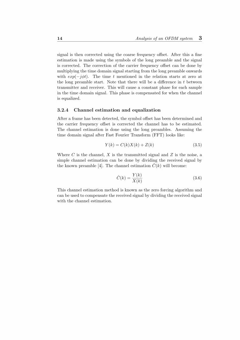
3.2.4 Channel estimation and equalization

After a frame has been detected, the symbol offset has been determined andthe carrier frequency offset is corrected the channel has to be estimated.The channel estimation is done using the long preambles. Assuming thetime domain signal after Fast Fourier Transform (FFT) looks like:

Y (k) = C(k)X(k) + Z(k) (3.5)

Where C is the channel, X is the transmitted signal and Z is the noise, asimple channel estimation can be done by dividing the received signal bythe known preamble [4]. The channel estimation C(k) will become:

C(k) =Y (k)X(k)

(3.6)

This channel estimation method is known as the zero forcing algorithm andcan be used to compensate the received signal by dividing the received signalwith the channel estimation.

3.2 Receiver tasks 15

3.2.5 Residual carrier frequency offset

Even after the carrier frequency offset has been compensated for and afterthe channel is equalized still some residual carrier frequency offset may exist.The residual CFO contained in the received signal may very well be time-varying and thus needs to be continuously tracked [3]. The residual CFOcauses phase distortions of the OFDM symbol in the frequency domain.Assuming that the CFO is constant for the received signal the residual CFOwill increase proportional to the symbols, this can be seen in Figure 3.5where θs is the initial phase and θd is the phase increase per symbol [2].Note that the residual CFO can also decrease proportional to the symbols.

dθ

dθ

dθ

sθ

0 1 2 3 Symbol Number t

Phas

e D

isto

rtio

n ( )tθ

Â

Figure 3.5: Residual carrier frequency offset [2]

The total residual phase of symbol number t would be:

θ = θs + tθd (3.7)

To compensate for the residual CFO the frequency domain signal is multi-plied with exp(−jθ).

4

Simulations

Before testing the digital system implementation on the MIMO testbed sim-ulations are done first. These simulations are done in order to test theprincipal of OFDM and to optimize parameters. This chapter gives a expla-nation about how the simulations are done. The results of the simulationswill not be presented in a separate chapter but are presented and discussedon the go. All simulations are done using the high-level technical computinglanguage Matlab.

The simulation of the OFDM system is divided into two parts, the re-ceiver and the transmitter respectively. At first all blocks will be individuallytested, to avoid dependencies on other blocks. This is to ensure that if ablock is modified not all dependant blocks have to be tested again. If allblocks work they will be tested as a whole. Also at first only noise is addedand later the channel model will be used in the simulations.

This chapter is divided into three sections, the first section will deal withthe transmitter simulations. This is followed by a section about the receiversimulations. And finally the last section describes the chain of transmitterand receiver combined.

4.1 Transmitter software blocks

This section will describe some tasks which are typically done by the trans-mitter side. The tasks include the generation of preambles and the assem-bling of frames. The tasks are described in the coming two subsections.

4.1.1 Preamble generation

Before the frames can be assembled the preamble has to be constructed.This is done using the sequences mentioned in the 802.11a standard. Onlythe creation of the short preamble will be described here, the long preambleis done in exactly the same manner. A piece of code describing the genera-

17

18 Simulations 4

preamble = [ ] ;symbol = ze ro s ( 1 , 6 4 ) ;symbol ( 2 : 2 7 ) = Tshort ( 2 8 : 5 3 ) ;symbol ( 3 9 : 6 4 ) = Tshort ( 1 : 2 6 ) ;% Power norma l i s a t i onsymbol = (64/ sq r t (2∗12) )∗ symbol ;symbol = i f f t ( symbol ) ;% ten t imes 16 samplespreamble = [ symbol symbol symbol ( 1 : 3 2 ) ] ;

Listing 4.1: Short preamble generation

% Random b i t sequencedata = randint ( Nframes∗SymbolsPerFrame , 52 , 2 ) ;% BPSK modulationdata = 2∗data −1;

Listing 4.2: BPSK modulation

tion of the short preamble can be seen in Listing 4.1. The variable Tshortcontains the symbols of the short preamble.

4.1.2 Frame generation

The preambles described in the previous section are appended to the frames.Each frame will consist of a ’gap’, the preambles and the data symbols. Thedata is BPSK modulated, which is very easy to implement in Matlab ascan be seen in Listing 4.2. Note that each row represents a data symbolto be transmitted and has a length of 52 OFDM symbols. A single framecan contain more then one data symbol, this is taken into account whengenerating the frame. Later on QPSK will be used when actually transmit-ting and demodulating data. The QPSK modulation is done by using theMatlab Modem Object. This object can take care of the modulation anddemodulation of several types. A short snippet of code describing the QPSKmodulation can be seen in Listing 4.3. Note that there is an extra factor

% Random b i t sequencedata = randint ( Nframes∗SymbolsPerFrame ∗52∗2 , 1 , 2 ) ;% QPSK modulationh = modem.qammod( ’M’ , 4 , ’ InputType ’ , ’ Bit ’ ,

’ SymbolOrder ’ , ’Gray ’ ) ;data = modulate (h , data ) ;data = reshape ( data , 52 , Nframes∗SymbolsPerFrame ) ’ ;

Listing 4.3: QPSK modulation

4.2 Receiver software blocks 19

two in the random data generation, this is because the modulation works asa kind of compression. After modulation there are 52 symbols left over. Itis needed to reshape the data because when modulating a multi-dimensionalarray Matlab assumes the columns are individual channels and the rows aretimestamps.

During simulation average white Gaussian noise (AWGN) is added tothe frames. Optionally also a channel model is applied to the frames. Thisis done by convolving the frame with a row from the ’Channel Model A’ dataset. During simulation no pilots are added to the signal, but when testingon the testbed pilots are added to the signal. As a consequence of this thesimulations will use 52 data bits whilst the testbed measurements will use48 data bits. This leaves four positions open which will be used as pilots.

4.1.3 Carrier frequency offset

After the addition of noise the last thing which is added to the signal isfrequency offset. This is done by multiplying the time domain signal withexp(φt) as can be seen in Listing 4.4.

phase = 2∗( p i /180 ) ;t = 0 : l ength ( frame )−1;frame = frame .∗ exp ( i ∗phase .∗ t ) ;

Listing 4.4: Adding carrier frequency offset

In this listing a phase of two degrees is successively added to the signal, thusthe first sample does not have a phase offset, the second sample has a phaseoffset of two degrees, the third sample has a phase offset of four degrees etc.When assuming a symbol time of 3.2 µs this result into a ∆f of 1.7 kHz.

4.2 Receiver software blocks

This section will describe some tasks which are typically done by the receiverside. These tasks include the timing offset detection, channel and frequencycorrection and the demodulation.

4.2.1 Frame detection

To compare all three frame detection algorithms mentioned in Section 3.2.1 atest was done using different signal-to-noise ratios. The signal-to-noise ratiowas varied between -20 and 20 dB. For each signal-to-noise ratio a thousandframes were tested to obtain the percentage of correctly detected frames.For each of the three frame detection methods a window size of sixteen wasused. A frame was considered correctly detected if it was detected before thethird last symbol of the short preamble and forty samples before the start ofthe frame. The region previously described can be seen in Figure 4.1. Both

20 Simulations 4

Figure 4.1: Correct frame detection region

the power detection method and the autocorrelation detection method needsixteen successive increases in their output before the signal is classified asa frame. The results of all three methods when no channel model is usedcan be seen in Figure 4.2. The frame detection ratio mentioned in the

Figure 4.2: Comparison of several frame detection methods with no channelmodel applied

figure is the percentage of detected frames to the total amount of frames.It can be seen from the figure that the noise power method has a far betterperformance compared to the other two detection methods. In Figure 4.3the results of all three frame detection methods are shown when using achannel model. It can be seen that the performance slightly decreases. Ina real life situation it is not known whether the received signal consists offrames, noise, or a combination of both. This may lead to situations werea received signal is falsely classified as a frame. To test how many framesare falsely detected a thousand frames consisting of only noise are testedto see if they are detected as frame. The noise level was varied between-20 dB and 20 dB and no channel model was used. The results showedthat the threshold detection method was the worst, on average roughly 92%

4.2 Receiver software blocks 21

−20 −15 −10 −5 0 5 10 15 200

20

40

60

80

100

SNR (dB)

Fra

me

dete

ctio

n ra

tio (

%)

Power detectionAutocorrelation detectionThreshold detection

Figure 4.3: Comparison of several frame detection methods with channelmodel applied

P = abs (P) ;po i = percentage ∗max(P) ; % Our po int o f i n t e r e s t[ r te , pos ] = min ( abs (P − poi ) ) ;

Listing 4.5: Sample index determination

of noise frames were detected as an actual frame. The other two methodsperformed much better. Using the correlation based detection only 0.31% ofthe frames were falsely detected and the power detection method performeda little better were only 0.17% of all frames were falsely detected.

The high number of falsely detected frames for the noise power thresholdmethod can be explained. When only comparing the averages of noise toeach other, the chance is very high that their is an average which is slightlyhigher. This will result to a falsely detected frame. An improvement wouldbe not to compare the averages to each other but to move the threshold afew standard deviations to the right.

4.2.2 Coarse detection

All three methods for coarse timing estimation, which are mentioned inSection 3.2.2, are compared with each other for values of signal-to-noiseratio between 0 dB and 10 dB. For each signal-to-noise ratio a thousandframes are tested. After determining the value at which the autocorrelationhas decreased by the given percentage the corresponding sample index hasto be determined. This is done by subtracting the value from the rest of thesignal and looking where the difference is the smallest. To elaborate this thecorresponding code snippet is given in Listing 4.5. In this listing P representsthe autocorrelation of the signal. The poi is the percentage of the maximumvalue. The corresponding sample index is now found by subtracting the

22 Simulations 4

P = abs (P) ;% Our po int o f i n t e r e s tpo i = percentage ∗max(P) ;r t e = abs (P − poi ) ;tmp = r t e < 0 .5∗mean( r t e ) ;tmp = f i nd (tmp ) ;i f isempty (tmp)

[ rte , pos ] = min ( r t e ) ;e l s e

pos = tmp ( 1 ) ;end

Listing 4.6: New sample index determination

autocorrelation output and the poi and looking at the minimum value ofthe result.

As can be seen the above mentioned method looks at the minimumvalue after subtraction. There might be a possibility that the minimumvalue does not correspond to the wanted value but to noise. The improvedmethod solves this issue by looking at the first occurrence where the errorvalue is smaller then half the average error. If this is not found it willjust use the old method to find the sample index. The principle can beseen in Listing 4.6. The results can be seen in Figure 4.4. The figureshows the percentage of frames were the coarse position has been correctlydetected. From the figure it can be seen that the improved max method

Figure 4.4: Comparison of the three different methods of coarse positiondetection, no channel model applied

and the method by Wang almost perform equally well. For both methods

4.2 Receiver software blocks 23

based on the maximum principle a correct detection was registered if thedetected position lays in the second last symbol of the short preamble. Forthe method of Wang a correct detection was registered if the symbol timewas off at maximum eight samples from the start of the second last symbolof the short preamble.

The same test as above was repeated, but this time using a channelmodel. The results using can be seen in Figure 4.5. It can be seen that

Figure 4.5: Comparison of the three different methods of coarse positiondetection, with channel model applied

the Wang method performs significantly worse when compared to the othermethods. The method which will be used for the rest of the simulations willbe the improved max function.

To test whether false detections occur of the coarse positions framesconsisting of different values of noise are tested. For each value of noisein the range of 0 dB to 10 dB ten thousand frames are tested without thechannel model. The improved max function does not falsely detect anypositions. The old max function falsely detects coarse positions in 9% ofthe cases. The method of Wang falsely detects the positions in 11% of thecases.

4.2.3 Fine detection

The fine detection is the last step and determines the symbol time offset.The fine peak algorithm needs a coarse position so that it knows where tolook. For the coarse position in the simulation an arbitrary position of 137was chosen. In the simulation ten thousand frames were used per differentvalue of signal-to-noise ratio. The signal-to-noise ratios were varied between

24 Simulations 4

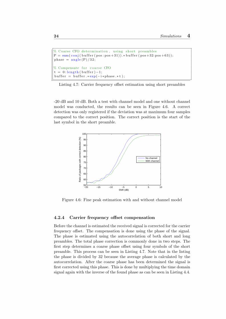
% Coarse CFO determinat ion , us ing shor t preamblesP = sum( conj ( bu f f e r ( pos : pos +31)) .∗ bu f f e r ( pos+32: pos +63)) ;phase = angle (P)/32 ;

% Compensate f o r coa r s e CFOt = 0 : l ength ( bu f f e r )−1;bu f f e r = bu f f e r .∗ exp(− i ∗phase .∗ t ) ;

Listing 4.7: Carrier frequency offset estimation using short preambles

-20 dB and 10 dB. Both a test with channel model and one without channelmodel was conducted, the results can be seen in Figure 4.6. A correctdetection was only registered if the deviation was at maximum four samplescompared to the correct position. The correct position is the start of thelast symbol in the short preamble.

−20 −15 −10 −5 0 5 1055

60

65

70

75

80

85

90

95

100

SNR (dB)

Rat

io o

f pac

kage

s w

ith c

orre

ct d

etec

tion

(%)

No channelWith channel

Figure 4.6: Fine peak estimation with and without channel model

4.2.4 Carrier frequency offset compensation

Before the channel is estimated the received signal is corrected for the carrierfrequency offset. The compensation is done using the phase of the signal.The phase is estimated using the autocorrelation of both short and longpreambles. The total phase correction is commonly done in two steps. Thefirst step determines a coarse phase offset using four symbols of the shortpreamble. This process can be seen in Listing 4.7. Note that in the listingthe phase is divided by 32 because the average phase is calculated by theautocorrelation. After the coarse phase has been determined the signal isfirst corrected using this phase. This is done by multiplying the time domainsignal again with the inverse of the found phase as can be seen in Listing 4.4.

4.2 Receiver software blocks 25

LP t = bu f f e r ( LP start : LP start +63);tmp = f f t ( LP t ) ;LP f ( 1 : 2 6 ) = tmp ( 3 9 : 6 4 ) ;LP f ( 27 : 5 2 ) = tmp ( 2 : 2 7 ) ;H = LP f . / Tlong ;

Listing 4.8: Channel estimation

The fine phase estimation is done in the same manner as the coarse phaseestimation, but this time the two long preamble symbols are used.

4.2.5 Channel estimation and equalization

After the carrier frequency offset correction the channel estimation is done bydividing the frequency domain representation of the received long preamblewith the actual frequency domain representation of the long preamble. Thecode listing can be seen in Listing 4.8. In the code listing LP t represents thetime domain representation of the long preamble and LP f represents thefrequency domain representation. This is divided by the actual frequencydomain representation which is represented by T long in the code to obtainthe channel estimation. In Figure 4.7 a constellation diagram of a singleOFDM data symbol is plotted before and after channel equalization. QPSKmodulation was used here and the signal-to-noise ration was 20 dB. Theimage on the left shows the constellation diagram of an uncompensatedOFDM symbol. The image on the right shows the constellation after channelcompensation and the four quadrants can clearly be seen.

−20 −10 0 10 20−20

−15

−10

−5

0

5

10

15

20

In−phase amplitude

Qua

drat

ure

ampl

itude

−2 −1 0 1 2−2

−1.5

−1

−0.5

0

0.5

1

1.5

2

In−phase amplitude

Qua

drat

ure

ampl

itude

Figure 4.7: Constellation diagram of an OFDM symbol, before and afterchannel equalization

26 Simulations 4

4.2.6 Demodulation

The demodulation of the signal is taken care of by the Matlab modem ob-ject. The demodulation object must match the one which is used in themodulation phase. To get a global idea about how the demodulation objectcan be used Listing 4.9 is provided.

demodObject = modem. qamdemod( ’M’ , 4 , ’ SymbolOrder ’ , ’ gray ’ ,’OutputType ’ , ’ b i t ’ ) ;

z = demodulate ( demodObject , symbol ’ ) ;

Listing 4.9: QPSK demodulation object

The symbol mentioned in the code is a singe OFDM symbol which has theguard interval removed and has been channel corrected. Later on the carrierfrequency offset will be introduced to the signal and will also be compensatedfor.

4.3 Integration

This chapter describes the integration of all above mentioned simulationpieces. During testing it became clear that the frame detection was notworking properly. The frames were detected too early, resulting in a mal-function of the coarse detection algorithm. This malfunction is caused bythe fact that the rising slope of the autocorrelation is present. When lookingat the percentage of the maximum value of the autocorrelation a value maybe detected which lies in the rising slope region of the autocorrelation. Therising slope can clearly be seen in Figure 3.2. To avoid this problem theframe position is manually set and everything works remarkably well as canbe seen in Figure 4.8. To generate this figure the signal-to-noise ratio wasvaried between -5 dB and 15 dB, for each noise level a thousand frames weretested. Note that the results used for this figure did not use the channelmodel yet. The figure shows both the amount of coarse peak detections,and the amount of fine peak detections. It can be seen that both lines arenearly equal meaning that if the coarse peak detection fails also the finepeak detection fails. When the channel model is enabled the results can beseen in Figure 4.9. It is remarkable to see that there is a difference betweenthe two lines, meaning that if the coarse detection fails there is a possibilitythat the fine detection does succeed.

4.3.1 Bit error rates

An interesting measurement in the communications world is the bit errorratio (BER). The BER is the number of bit errors divided by the totalnumber of bits transmitted. This test was also done in the simulations, onewith no channel model and one with a channel model. To obtain the results

4.3 Integration 27

−5 0 5 10 150

20

40

60

80

100

SNR (dB)

Cor

rect

det

ectio

n (%

)

CoarseFine

Figure 4.8: Fine and coarse detections without channel model

−5 0 5 10 150

10

20

30

40

50

60

70

80

90

100

SNR (dB)

Cor

rect

det

ectio

n (%

)

CoarseFine

Figure 4.9: Fine and coarse detections with channel model

the signal-to-noise ratio was varied between -5 dB and 15 dB and for eachsignal-to-noise level a thousand frames with ten symbols each were tested.This time also QPSK modulation is used, and the frame start is manuallyset, as the frame detection method does not work well. The results can beseen in Figure 4.10.

−5 0 5 10 1510

−8

10−6

10−4

10−2

100

SNR (dB)

Bit

Err

or R

ate

ChannelNo channel

Figure 4.10: Bit error rates with and without the channel model applied

5

Test setup

After the simulations the OFDM principal is tested in real life on theMultiple-Input Multiple-Output (MIMO) testbed. The real-time MIMOtestbed enables researchers to test algorithms in a real-world office situa-tion, to change environment conditions and add or remove processing powerin a flexible fashion [10].

5.1 Testbed description

The testbed is able to transmit and receive four channels simultaneouslyand has a modularized setup. The setup consist of two trolleys which actas the transmitter and receiver. The transmitting trolley contains a digitalto analog converter, a up-converter, a RF amplifier and an UninterruptiblePower Supply (UPS) so that also over large distances can be transmitted.The receiver trolley contains a down-converter and a analog to digital con-verter. Both transmitter and receiver have a data buffer. The transmitterwill continuously transmit the contents of the buffer and at the receiver sidethe data can be captured into the buffer and can be read into the computeras a raw stream file.

In the following sections the blocks in the test setup images correspond tothe physical blocks present on the trolleys. This done to keep things simple,but might also be somewhat misleading. For example, the down-converteralso contains a low pass filter.

5.2 Test method

The baseband signals are generated by the Matlab code and have to be firstconverted to an IT++ file. This IT++ file is later converted to a raw streamfile by a custom piece of C++ software. The raw stream file is then loadedinto the data buffer of the transmitter. The received data is also in the rawstream format and is first converted to the IT++ format which then can be

29

30 Test setup 5

converted back to a Matlab readable format. The data conversion betweenthe IT++ format and the Matlab variable format is done by two Matlabscripts called itload.m and itsave.m respectively. These files are providedby the IT++ project [1]. The experiments will be done in a progressivemanner. This means that first a signal is transmitted at baseband this isfollowed by a signal which is up converted and then down converted againand finally if everything works the signal is transmitted through the air.Each of the tests will be done using three different modulation scheme whichhave an increasing difficulty to detect. The three modulation schemes are,in order of difficulty, BPSK, QPSK and Quadrature Amplitude Modulationusing sixteen symbols (QAM16). Each of the experiments will be describedbriefly in the following subsection. The blocks which are depicted in thefigures correspond to the physical blocks which are present on the MIMOtestbed.

5.2.1 Baseband

First only the baseband transmission is done, this means the signal has notbeen mixed up to the carrier frequency and transmitter and receiver aresill connected by a wire. The system setup can be seen in Figure 5.1. The

Figure 5.1: Baseband setup

computer on the left will act as the transmitter and will place the data in thetransmission buffer. The buffer is read out by the digital-to-analog converter(DAC) and produces an in-phase (I) and a quadrature (Q) baseband signalper channel. The output of the DAC is attached to the I and Q inputs ofthe analog-to-digital converter, which will write the received data to anotherbuffer. This buffer can be read out with the computer on the receiver side.

5.3 Test results 31

5.2.2 Up and down

The next step is to up and down convert the signal in the transmissionpath. The transmitter and receiver are still connected to each other usinga cable. The setup can be seen in Figure 5.2. The blocks with an arrow

Figure 5.2: Setup using mixers

symbol represent the mixers. These mix the baseband signal with the carrierfrequency.

5.2.3 Air

The last and final step will transmit the data through the air. The setup canbe seen in Figure 5.3. Note that there is a power amplifier (PA) attached to

Figure 5.3: Real world setup

the DAC, this is because the DAC can not produce enough power by itselffor transmission.

5.3 Test results

The test results which were obtained from the testbed were not as expected.The problem might be the testbed or the baseband data which is generatedby the Matlab script. As time was a critical issue the testbed results ofXiaoying Shao were used instead. These results only contained QPSK andQAM16 modulated data.

Each measurement contained seven packets which consisted of 16 frames,this means that for each measurement 112 frames are demodulated. Thenumber of OFDM symbols per frame for QPSK modulated data was 128and for QAM16 modulated data was 64. This was to ensure that the sameamount of bits were transmitted for each modulation type. Each transmit-ted packet contained the same data. The OFDM data symbols contained

32 Test setup 5

pilots, this was needed to compensate for the residual carrier frequency off-set. Especially the QAM16 modulated signals were effected by this effect.The tests which used a carrier frequency the frequency was set to 2.3 GHz.This frequency was chosen to avoid any interferences with existing WLANtransmitters which use a carrier frequency of 2.4 GHz. An external localoscillator was used for both the ADC and the DAC as the internal oscillatordoes not work well. The Automatic Gain Control (AGC) of the receiver wasalso adjusted by hand as it did not function properly.

The initial idea was to transmit a single frame and do the frame detectionby hand as the frame detection algorithms which were tested did not workproperly. Because the data of Xiaoying contained seven packets with 16frames it would be very laborious to do the frame detection by hand foreach frame. A very simple frame detection method was used which comparedthe instantaneous power of the received signal to predefined threshold. Thismethod could be used because the signal-to-noise ratio (SNR) of the receivedsignals was very high. The magnitude of a received QPSK modulated signalcorresponding to the start of a frame can be seen in Figure 5.4. From thefigure it can clearly be seen that the SNR is high and that the received signalshows some repetition.

50 100 150 200 250 300 350 400 450 5000

1

2

3

4

5

6

7

Sample index

Mag

nitu

de

Figure 5.4: Magnitude of a received QPSK modulated signal

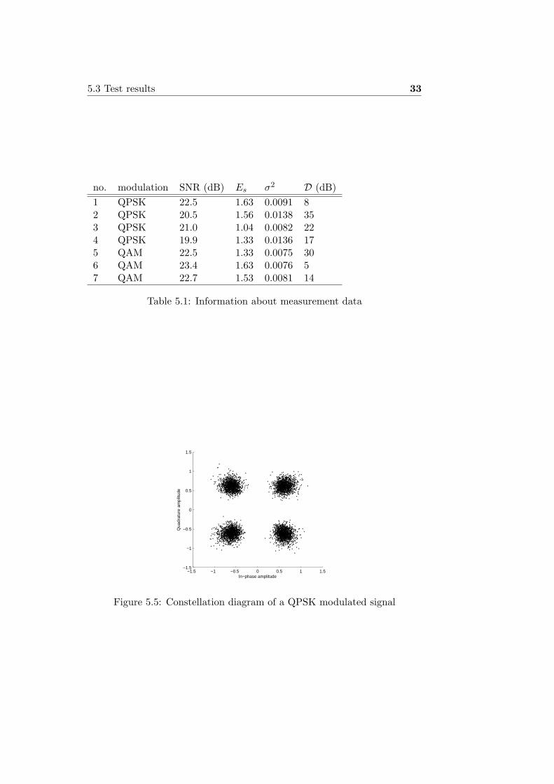
The measurement data consisted of seven sets. The most importantparameters of these sets are summarized in Table 5.1. This table showsthe type of modulation used, the estimated signal-to-noise ratio which iscalculated from the mean energy of the signal (Es) and the variation (σ2).The dynamic range of the channel is also mentioned and is depicted by theD symbol.

A constellation diagram of the first frame of a QPSK modulated signalcan be seen in Figure 5.5. The constellation points do not show any overlapwith other constellation points, this means the data can be recovered errorfree.

5.3 Test results 33

no. modulation SNR (dB) Es σ2 D (dB)1 QPSK 22.5 1.63 0.0091 82 QPSK 20.5 1.56 0.0138 353 QPSK 21.0 1.04 0.0082 224 QPSK 19.9 1.33 0.0136 175 QAM 22.5 1.33 0.0075 306 QAM 23.4 1.63 0.0076 57 QAM 22.7 1.53 0.0081 14

Table 5.1: Information about measurement data

−1.5 −1 −0.5 0 0.5 1 1.5−1.5

−1

−0.5

0

0.5

1

1.5

In−phase amplitude

Qua

drat

ure

ampl

itude

Figure 5.5: Constellation diagram of a QPSK modulated signal

34 Test setup 5

A constellation diagram of the first frame of a QAM modulated signalcan be seen in Figure 5.6. It can be seen that the complete constellationdiagram is turned a bit to the left. This is caused by some constant carrierfrequency offset which has not been removed properly.

−1.5 −1 −0.5 0 0.5 1 1.5−1.5

−1

−0.5

0

0.5

1

1.5

In−phase amplitude

Qua

drat

ure

ampl

itude

Figure 5.6: Constellation diagram of a QAM modulated signal

A plot of the mean phase of the pilots of the first five frames of thesecond measurement can be seen in Figure 5.7. The abrupt changes inphase correspond to the different frames.

0 100 200 300 400 500 600 700

−80

−60

−40

−20

0

20

40

60

80

Pha

se [d

egre

es]

Sample index

Figure 5.7: Mean phase of the pilot signals

To test the robustness of the developed Matlab scripts some artificialnoise was added to the noise because the measurement data already hashigh signal-to-noise ratios. Three different levels of noise were added, 15 dB,10 dB and 5 dB. Only three values were chosen because the Matlab demodu-lation script takes a long time to execute. For each of the measurements thebit error rate as a percentage was determined. The final results can be seenin Table 5.2. The first column in the table is the measurement, the numberis the same as the one used in Table 5.1. The second column are the biterror rates expressed as a percentage for the measurements without artificial

5.3 Test results 35

no. modulation no noise 15 dB 10 dB 5 dB1 QPSK 0,00 0,00 0,01 0,132 QPSK 1,60 1,80 2,16 3,433 QPSK 0,18 0,47 1,30 10,314 QPSK 0,16 0,24 0,48 4,755 QAM 3,05 4,08 5,77 10,696 QAM 1,16 1,53 2,37 4,927 QAM 2,06 2,88 4,73 9,47

Table 5.2: Bit error rates for various levels of artificial noise.

noise added. The following columns are the bit error rates, once again ex-pressed as a percentage, for measurements with artificial noise added. TheMatlab script which does the synchronization and demodulation takes aboutsix minutes to run on a 2.0 GHz Intel Core Duo.

An interesting fact to notice is that measurements were QAM modula-tion was used the bit error rates are slightly higher when compared to themeasurements were QPSK modulation was used. This is possibly causedby the fact that the signal-to-noise ratio of the QAM measurements arehigher 5.1.

6

Conclusions andrecommendations

6.1 Conclusions

The results from the simulation show that algorithms developed to carry outthe different tasks in the OFDM system like the preamble and frame gener-ation, frame detection and channel estimation and equalization are working.Some of the modules like the frame detection need some adjustment to im-prove the detection rate. The improved max detection method appears tobe the most efficient method for detecting the coarse position.

The developed Matlab software has a modular setup such that new partscan easily be developed, tested and implemented. The software implemen-tation which does the synchronization and demodulation of the receivedsignals is working in real life situations. The bit error rates which have beenachieved on the MIMO testbed are between 0 % and 3,05 % for signals witha signal-to-noise ratio of roughly 20 dB. Now it is proven that the signal re-ceived by the MIMO testbed can be synchronized and demodulated. Futuredevelopment of various algorithms can be carried out easily on the MIMOtestbed.

6.2 Recommendations

Some recommendations for future work are listed below.

• Eliminate the need to do file conversions manually, at the moment twofile conversions are done before the measurement data can be importedinto Matlab.

• Decrease the execution time of the Matlab script. The current Mat-lab script takes six minutes to execute at the moment for a singlemeasurement.

37

38 Conclusions and recommendations 6

• A frame detection algorithm which performs well under low signal-to-noise ratios and that is not dependant on a threshold.

• Extend the Matlab scripts such that they also work for the MIMOcase.

Bibliography

[1] IT++. http://apps.sourceforge.net/wordpress/itpp.

[2] K. Akita, R. Sakata, and K. Sato. A phase compensation scheme us-ing feedback control for ieee 802.11a receiver. In Vehicular TechnologyConference, 2004. VTC2004-Fall. 2004 IEEE 60th, volume 7, pages4789–4793 Vol. 7, Sept. 2004.

[3] T. Chieh and P. Tsai. OFDM Baseband Receiver Design for WirelessCommunications. John Wiley & Sons (Asia) Pte Ltd, 2007.

[4] Y. Chiu, D. Markovic, H. Tang, and N. Zhang. OFDM Receiver Design.PhD thesis, Berkeley, 2000.

[5] ETSI. Digital Video Broadcasting (DVB); Framing structure, channelcoding and modulation for digital terrestrial television, 01 2001.

[6] O. Filth. File:OFDM receiver ideal.png, 2009. http://en.wikipedia.org/wiki/File:OFDM_transmitter_ideal.png.

[7] IEEE. 802.11a-1999 High-speed Physical Layer in the 5 GHz Band,2008.

[8] J. Medbo and P. Schramm. Channel models for HIPERLAN/2 in differ-ent indoor scenarios. Technical Report 3ERI085B, ETSI/BRAN, Mar.1998.

[9] T.M. Schmidl and D.C. Cox. Robust frequency and timing synchroniza-tion for ofdm. Communications, IEEE Transactions on, 45(12):1613–1621, Dec. 1997.

[10] X. Shao. The MIMO project, 2008. http://www.sas.el.utwente.nl/open/research/wireless_communication/MIMO.

[11] R. van Nee and R. Prasad. OFDM for Wireless Multimedia Communi-cations. Artech House, 2000.

39

40 Bibliography

[12] K. Wang, M. Faulkner, J. Singh, and I. Tolochko. Timing Synchroniza-tion for 802.11a WLANs under Multipath Channels.