Embed Size (px)
Citation preview

Erasmus Mundus Master Course: IMETE
Thesis submitted in partial fulfilment of the requirements for the joint academic degree of:
International Master of Science in Environmental Technology and Engineering
an Erasmus Mundus Master Course from
Ghent University (Belgium), ICTP (Czech Republic), UNESCO-IHE (the Netherlands)
Nitrification and denitrification by algal-bacterial biomass in a Sequential Batch Photo-bioreactor:
effect of SRT
Host university:
MSc Thesis by
Dudy Fredy
Supervisor Mentor
Prof. Piet Lens Dr. Peter van der Steen
Delft August 2013
This thesis was elaborated and defended at the UNESCO-IHE, Delft, The Netherlands within the
framework of the European Erasmus Mundus Programme “Erasmus Mundus International Master of
Science in Environmental Technology and Engineering " (Course N° 2011-0172)


Certification
This is an unpublished MSc. thesis and is not prepared for further distribution. The author and the
promoter give the permission to use this thesis for consultation and to copy parts of it for personal use.
Every other use is subject to copyright laws, more specifically the source must be extensively
specified when using results from this thesis.
The Promoter The Author
Prof. Piet Lens
Dudy Fredy

The findings, interpretations and conclusions expressed in this study do neither necessarily reflect the
views of the UNESCO-IHE Institute for Water Education, nor of the individual members of the MSc
committee, nor of their respective employers.

for Azzania and Dyaz


i
Abstract
A post-treatment of UASB reactor’s effluent by utilizing the interaction of algae and bacteria can offer
lower energy consumption via photosynthetic oxygenation. To meet a stringent standard effluent it is
necessary to optimize nitrogen removal. This research investigated the effects of Sludge Retention
Time (SRT) on nitrification and denitrification performance.
A mixed biomass culture of different species of microalgae and bacteria were inoculated in an open
photo-bioreactor. The 1-L reactor was illuminated (25.9 µmol/m2.s) and operated as a sequential
batch reactor at 28ºC and pH 7.5 with 50% discharge per cycle (2 cycles per day). SRT were varied
from 17 to 52 days by discharging different volume of completely mixed culture.
Nitrification and denitrification of artificial wastewater (23 mgN-NH4/L and 200 mg COD/L) were
achieved. The present study identified that SRT has only limited effect on the nitrification process and
uptake by algal-bacterial biomass in a photo-bioreactor. The overall removal rates only varies from 2.1
to 2.9 mgN-NH4/L.h , while SRT varies from 17 to 52 days. The maximum oxygen production was
occurred in SRT 17 days at a rate 0.3 mgO2/m3.day.
Keywords: algae, denitrification, nitrification, photo-bioreactor, photosynthetic oxygenation, SRT


iii
Acknowledgements
I would like to thank the almighty Allah for the uncountable blessing that He has bestowed upon me.
My sincerest appreciations go to Dr. Peter van der Steen. Thank you so much for your guidance, input,
throughout the research and thesis writing period. I am deeply grateful to Prof. Piet Lens for the advice
and input throughout thesis work.
Thank you to Angelica Rada and Rudatin Windaswara, for countless support, input and of course the
valuable data for completing this thesis.
I acknowledge Eldon Raj, Carlos Lopez Vazquez, and all the colleagues in paper writing meeting for
correction and suggestions towards the finalizing of this thesis. I also thank to my colleagues in algae
research: Indri Karya, Kuntarini Rahsilawati, Freweyni Tammene, and Thanh Tung Nguyen.
I would like to express my appreciation for the help and assistant of the laboratory staff at UNESCO-
IHE: Fred Kruis, Berend Lolkema, Peter Heering, Ferdi Battes, Frank Wiegman and Lyzette
Robbemont. I also would like to thanks to Laurens Welles, Javier Sánchez Guillén and Sondos Saad
who were very helpful during ‘great’ months in the lab.
The last and the most important, my wife Azzania. All is nothing without your support. Thank you for
your pray, understanding and sacrifices. And to my son Dyaz. You are my spirit keeper. Thank you.


v
Table of Contents
ABSTRACT ................................................................................................................................... I
ACKNOWLEDGEMENTS ............................................................................................................ III
1 INTRODUCTION .................................................................................................................. 1
1.1 Background ................................................................................................................ 1
1.2 Problem Statement ..................................................................................................... 2
2 LITERATURE REVIEW ........................................................................................................ 3
2.1 Post-treatment options of UASB reactor’s effluent ................................................... 3
2.2 Biological nitrogen removal from wastewater ........................................................... 4
2.2.1 Nitrification ............................................................................................................ 4
2.2.2 Denitrification ........................................................................................................ 5
2.2.3 Effect of C/N ratio on nitrogen removal ................................................................ 7
2.2.4 SRT (Solids Retention Time) ................................................................................. 7
2.2.5 Sequential Batch Reactor (SBR) ............................................................................ 8
2.3 Algal-bacterial consortium for wastewater treatment .............................................. 10
2.3.1 Microalgae ............................................................................................................ 13
2.3.2 Microalgae culture system ................................................................................... 13
2.3.3 Influence of environmental parameters on algal growth ...................................... 14
2.4 Effect of dark periode on nitrogen removal ............................................................. 17
3 OBJECTIVES ..................................................................................................................... 19
3.1 General objective ...................................................................................................... 19
3.2 Specific objectives .................................................................................................... 19
4 MATERIAL AND METHODS .............................................................................................. 21
4.1 Culture medium ........................................................................................................ 21
4.2 Microalgae-bacteria consortium ............................................................................... 22
4.3 Reactor set up and experimental design ................................................................... 22
4.4 Sampling ................................................................................................................... 24
4.5 Analytical Methods .................................................................................................. 24
4.5.1 Ammonium nitrogen ............................................................................................ 24
4.5.2 Nitrite nitrogen ..................................................................................................... 25
4.5.3 Nitrate nitrogen .................................................................................................... 25
4.5.4 Chlorophyll-a ....................................................................................................... 25
4.5.5 Total suspended solid (TSS) and volatile suspended solid (VSS) ....................... 26
4.5.6 Biomass Light Absorption ................................................................................... 26
4.6 Calculation ............................................................................................................... 26
4.6.1 Solid Retention Time (SRT) ................................................................................ 26
4.6.2 Nitrogen balance .................................................................................................. 27
4.6.3 Biomass composition ........................................................................................... 28
4.6.4 Oxygen production by algae ................................................................................ 29
4.7 Statistical analysis .................................................................................................... 31
4.8 Batch experiment ...................................................................................................... 31
5 RESULTS ........................................................................................................................... 33

5.1 Nitrogen removal ...................................................................................................... 33
5.1.1 Daily nitrogenous concentration .......................................................................... 33
5.1.2 Ammonium conversion rate ................................................................................. 34
5.2 Nitrogen balance ...................................................................................................... 35
5.3 Chlorophyll-a concentration ..................................................................................... 36
5.4 Suspended solids concentration ............................................................................... 37
5.5 Light absorption ....................................................................................................... 38
5.6 Biomass composition ............................................................................................... 39
5.7 Solids Retention Time (SRT) ................................................................................... 39
5.8 Oxygen production ................................................................................................... 41
5.9 Nitrate uptake batch experiment .............................................................................. 44
5.10 Microscopic observation .......................................................................................... 44
6 DISCUSSION ...................................................................................................................... 47
6.1 Ammonium conversion rate ..................................................................................... 47
6.2 The effects of different operational sequences in SBR ............................................ 48
6.3 The effects of different SRT in SBR ........................................................................ 49
6.4 Comparison with other algal-bacterial photo-bioreactor ......................................... 51
6.5 Development of biofilm in the reactor ..................................................................... 52
6.6 Light regime in photobioractor ................................................................................ 53
6.7 Denitrification .......................................................................................................... 54
7 CONCLUSION AND RECOMMENDATIONS ......................................................................... 55
7.1 Conclusion ................................................................................................................ 55
7.2 Recommendations .................................................................................................... 55
REFERENCES ............................................................................................................................ 57
APPENDIX A ............................................................................................................................. 63
APPENDIX B ............................................................................................................................. 73
APPENDIX C ............................................................................................................................. 84
APPENDIX D ............................................................................................................................. 92
APPENDIX E ............................................................................................................................. 93

vii
List of tables
Table 2.1: Typical average concentration of UASB reactor’s effluent ................................................... 3
Table 2.2: Summary of various UASB-post treatment systems and their average level of effluent
quality ................................................................................................................................. 3
Table 2.3: Different operational sequences of SBR operation ................................................................ 9
Table 2.4: Algal-bacterial consortium for nutrient removal from wastewater ...................................... 13
Table 4.1: Modified BG-11 medium for microalgae and bacteria culture ............................................ 21
Table 4.2: Experimental variations ....................................................................................................... 23
Table 4.3: SBR operational setting at period 1 ...................................................................................... 23
Table 4.4: SBR operational setting at period 2, 3 and 4 ........................................................................ 24
Table 5.1: Nitrogen removal efficiency................................................................................................. 33
Table 5.2: Summary of ammonium conversion rate in different period ............................................... 34
Table 5.3: Nitrogen balance based on one cycle operation in SBR ...................................................... 35
Table 5.4: Actual SRT calculation ........................................................................................................ 39
Table 5.5: Estimation of biomass composition ..................................................................................... 40
Table 5.6: Estimation of oxygen production and consumption rate in the reactor ................................ 43
Table 6.1: Comparison the result with other research ........................................................................... 51


ix
List of figures
Figure 1.1:Typical configuration of water treatment plant with UASB-Activated Sludge ..................... 1
Figure 2.1:Typical cycles in Sequential Batch Reactor ........................................................................... 9
Figure 2.2:Interaction between algae and bacteria in wastewater treatment process ............................ 11
Figure 2.3: Relation between light intensity on photoautotrophic growth of photosynthetic cells ....... 14
Figure 4.1: Schematic diagram of reactor set up ................................................................................... 22
Figure 4.2: DO concentrations profile partition in one cycle of SBR operation ................................... 29
Figure 5.1: Daily nitrogenous concentration ......................................................................................... 33
Figure 5.2: Ammonium conversion in one cycle of SBR operation in period 2 day 89 ....................... 34
Figure 5.3: Profile of chlorophyll-a concentration in different periods ................................................ 36
Figure 5.4: Average chlorophyll-a concentration in different periods .................................................. 36
Figure 5.5: Profile of SS concentration in different periods.................................................................. 37
Figure 5.6: Average SS concentration in different periods ................................................................... 37
Figure 5.7: Light intensity measurement points (a) and a simplified side view of the reactor (b) ........ 38
Figure 5.8: Estimated light penetration inside reactor ........................................................................... 38
Figure 5.9: Biomass compositions in each period ................................................................................. 39
Figure 5.10: Typical DO profile in one cycle operation in period 1(day 46) ........................................ 41
Figure 5.11: Typical DO profile in one cycle operation in period 2(day 68) ........................................ 42
Figure 5.12: Typical DO profile in one cycle operation in period 3 (day 117) ..................................... 42
Figure 5.13: Typical DO profile in one cycle operation in period 4 (day 171) ..................................... 43
Figure 5.14: Nitrate uptake performances by algae-bacteria consortium .............................................. 44
Figure 5.15: Chlorella sp. and Spirulina sp. (20x magnification) ......................................................... 44
Figure 5.16: Scnedesmus sp. and Anabaena sp. (40x magnification) ................................................... 45
Figure 5.17: Algal-bacterial flocs .......................................................................................................... 45
Figure 6.1: Volumetric productivity of a photobioreactor rUx as a function of biomass concentration Cx
.......................................................................................................................................... 50
Figure 6.2: Attached thread-former species of microalgae in reactor’s wall ........................................ 53
Figure 6.3: Light fraction as function of the chlorophyll-a concentration in the reactor ...................... 53
Figure 6.4: Typical nitrogen concentration profile within a cycle (Day 117) ....................................... 54


xi
Abbreviations and symbols
AOB Ammonia-oxidizing Bacteria
BOD Biochemical Oxygen Demand
BNR Biological Nitrogen Removal
C/N Carbon/Nitrogen
Chla Chlorophyll a
COD Chemical Oxygen Demand
DO Dissolved Oxygen
FA Free Ammonia
FNA Free Nitrous Acid
FSA Free Saline Ammonia
HRAP High Rate Algal Ponds
HRT Hydraulic Retention Time
N Nitrogen
NOB Nitrite-oxidizing Bacteria
OD Optical Density
P Phosphorus
PBR Photobioreactors
SBR Sequencing Batch Reactor
SRT Solid(sludge) Retention Time
TKN Total Kjeldahl Nitrogen
TN Total Nitrogen
TP Total Phosphorus
TSS Total Suspended Solid
UASB Upflow Anaerobic Sludge Blanket
VSS Volatile Suspended Solid
WSP Waste Stabilization Ponds
WWTP Wastewater Treatment Plant


Dudy Fredy 1
1 Introduction
1.1 Background
High-rate anaerobic treatment system especially Upflow Anaerobic Sludge Blanket (UASB) reactor is
popularly used for sewage treatment in tropical and developing countries (Seghezzo et al., 1998;
Gomec, 2010). It is a sustainable technology and offers some advantages such as low cost, low energy
consumption and simple operation (Chernicharo, 2006; Khan et al., 2011). However, the effluents of
anaerobic reactor require a post-treatment to meet stringent discharge standards, especially the
Nitrogen concentration in the effluent. Various technological options for further treating the UASB’s
effluent are available to achieve desired effluent quality. One of the promising options is to couple
UASB with Activated Sludge System. A UASB-Activated Sludge system consists of a UASB reactor,
a continues-flow aerated bioreactor and a settler as shown in Figure 1.1. Many studies reported that
coupling UASB with Activated Sludge can achieve high removal of Biochemical Oxygen Demand
(BOD), Chemical Oxygen Demand (COD) and Total Suspended Solids (TSS) (Chernicharo, 2006;
Chong et al., 2012).
Figure 1.1:Typical configuration of water treatment plant with UASB-Activated Sludge
Source: (Chernicharo, 2006)
As a variant of activated sludge system, Sequential Batch Reactor (SBR) can be coupled with UASB
(Chong et al., 2012). In SBR, treatment of wastewater is carried out in various consecutive phases
such as filling, reaction, settling, decant, and idle, within one reactor. SBR adds up the benefit on
smaller footprint requirement.
On the other hand, microalgae have been used to treat wastewater for many years in large ponds and
photo-bioreactors. Microalgae have high affinity for nitrogen and phosphorous, and do not require
much an organic carbon source (Boelee et al., 2012). The use of microalgae for wastewater treatment

2 MSc Thesis
becomes more attractive as wastewater can be a nutrient supply for microalgal biofuel production.
This will bring the biofuel production more economically viable and sustainable (Boelee et al., 2011).
A combination treatment of wastewater, by utilizing the interaction of algae and bacteria can offer
lower energy consumption via photosynthetic aeration. Microalgae provide the oxygen necessary for
aerobic bacteria to biodegrade organic pollutants and ammonium removal, Furthermore, the
application of algal-bacterial system in a Sequential Batch Photo-bioreactor as a post-treatment for
domestic wastewater can show a great potential. It will reduce aeration cost and land requirement,
which are the major problems in developing countries.
1.2 Problem Statement
Nitrification and denitrification are the main pathways for nitrogen removal in wastewater treatment.
In the algal-bacterial system, nitrogen accumulation into algal biomass could also contribute to the
removal process. Previous research (Karya et al., 2013) identified a stable consortium of algae
(Scenedesmus) and nitrifiers that could be established in a photo-bioreactor. It was found that
nitrification could takes place at rates up to 8.5 mg/L.h. The in-situ oxygen generation by algae was
found to be more than sufficient for the nitrification process (Karya et al., 2013).
Beside nitrification, denitrification should also be introduced in the reactor to achieve high quality of
effluent. The removal of nitrogen in the SBR system can be achieved by alternating aerobic and
anoxic periods during the reaction. In photo-bioreactor anoxic periods can be done by creating dark
periods or dark zones. Another study (Windraswara, 2013) identified that denitrification can occur in
algal-bacterial system in a photo-SBR, when no lights was applied in the anoxic periods.
With a more stringent standard effluent for total nitrogen, it is necessary to establish a good nitrogen
removal in Sequential Batch Photo-bioreactor. The nitrogen removal efficiency is influenced by a
number of factors, such as sludge age, temperature, and carbon availability. The focus of this research
therefore is to investigate the effects of sludge age or Sludge Retention Time (SRT) on nitrification
and denitrification performance.

Dudy Fredy 3
2 Literature review
This chapter describes background information of post-treatment options for UASB reactor’s effluent,
conventional biological nitrogen removal, and algal-bacterial interactions in wastewater treatments.
2.1 Post-treatment options of UASB reactor’s effluent
High-rate anaerobic treatment system especially UASB reactor receives great interests for sewage
treatment in tropical and developing countries (Seghezzo et al., 1998; Gomec, 2010). It offers some
advantages such as low cost, low energy consumption and simple operation (Chernicharo, 2006).
However, the effluents of anaerobic reactor require further post-treatment to meet stringent discharge
standards. A typical average effluent concentration from UASB reactor is shown in Tabel 2.1.
Table 2.1: Typical average concentration of UASB reactor’s effluent
Parameter Concentration (mg/L) BOD5 70-100 COD 180-270 TSS 60-100 Ammonia >15 Total N >20 Total P >4
Source: (Chernicharo, 2006)
Many studies on finding the suitable post-treatment have been done. Chong et al., (2012) thoroughly
reviewed the most common options for UASB reactor effluent treatments. The summary of various
UASB-post treatment systems and their effluent quality can be seen in Table 2.2. The main goal of
adopting a post-treatment system to treat an anaerobic effluent is to find a process that is simple in
operation and maintenance, lower capital costs, and energy efficient.
Table 2.2: Summary of various UASB-post treatment systems and their average level of effluent quality
Post-treatment Unit BOD
(mg/L) COD
(mg/L) TSS
(mg/L) Ammonia
(mg/L) TKN
(mg/L)
Total
N
(mg/L)
Total
P
(mg/L) Activated sludge (AS) 7 47 13 3 no data no data no data
Sequencing-batch reactor (SBR) 5 37 12 0.5 10 no data 1.3 Biofilter (BF) 31 70 21 20 20 no data no data
Downflow-hanging sponge (DHS) 8 57 28 13 no data 34 no data
Stabilising pond (SP) 33 110 60 7.6 no data 9.6 2.1 Series Rotating-biological contactor
(RBC)
no data 56 no data 13 8 no data no data
Constructed wetland (CW) 17 47 12 17 36 33 1.9 Source : Adapted from (Chong et al., 2012)

4 MSc Thesis
Based on Table 2.2, the coupling of a post treatment unit to a UASB reactor is effective at removing
the residual organic matter and suspended solids. But, there is still a lack of studies on the removal of
nutrients (Total Nitrogen and Total Phosphorous concentrations). However for achieving a good
nitrogen removal, the organic matter removal efficiency of UASB reactor should be no more than 50–
70%, so that there is enough organic matter for the denitrification step (Chernicharo, 2006).
2.2 Biological nitrogen removal from wastewater
Activated sludge process is one of the most common methods for treating wastewater treatment, in
which nitrification and denitrification are the main pathways for nitrogen removal. Nitrification is a
two steps process carried out by two different autotrophic bacterial groups. In the first step ammonium
is oxidized to nitrite by ammonia oxidizing bacteria (AOB). In the second step nitrite is oxidized to
nitrate by nitrite oxidizing bacteria (NOB). For completing nitrogen removal, nitrate is reduced to
nitrogen gas in the denitrification process by heterotrophic bacteria.
2.2.1 Nitrification
The two sequential oxidation steps in nitrification are shown below as basic stoichiometric redox
reactions:
NH4+ + 1.5O2 NO2
- + H2O + 2H
+ (2.1)
NO2- + 0.5O2 NO3
- (2.2)
By stoichiometri the oxygen requirement for conversion of ammonia to nitrate is 4.57 mgO2/mgN
utilized.
In nitrification process, dissolved oxygen (DO) concentration is the most important parameter for both
AOB and NOB. Ammonia is fully oxidized to nitrate at DO concentrations higher than 1 mgO2/L
(Campos et al., 2007). Higher dissolved oxygen concentrations do not appear to affect nitrification
rates significantly, however low oxygen concentrations reduce the nitrification rate (Ekama and
Wentzel, 2008). Moreover, operation at DO concentrations of 0.6 and 0.4 mgO2/L can cause ammonia
and nitrite accumulations (Campos et al., 2007).
Furthermore, nitrification releases hydrogen ions and decreases alkalinity of the mixed liquor. For
each of mg FSA (Free Saline Ammonia) that is nitrified, 7.14 mg alkalinity (as CaCO3) is consumed.
When the alkalinity falls below about 40 mg/L as CaCO3 then, irrespective of the carbon dioxide
concentration, the pH becomes unstable and decreases to low values (Ekama and Wentzel, 2008).
Hence it is important to maintain a buffer of alkalinity in the aeration tank to provide pH stability and

Dudy Fredy 5
ensure the presence of inorganic carbon for nitrifying bacteria. The residual amount of alkalinity
desired in the aeration tank after complete nitrification is at least 50 mg/L (Gerardi, 2002).
It is reported that the optimum pH for AOB Nitrosomonas is 8.1 and for NOB Nitrobacter is 7.9
(Grunditz and Dalhammar, 2001). The AOB activity is 50% reduced at pH values of 6 and 10
(Jiménez et al., 2012) and NOB were strongly affected by low pH values (no activity was detected at
pH 6.5). And it is also reported that no inhibition was observed at high pH values (activity was nearly
the same for the pH range 7.5–9.95) (Jiménez et al., 2011).
Temperature has a significant effect on microbial nitrification activity. The rate of nitrification is
reduced with decreasing temperature and, conversely, there is a significant acceleration in the rate of
nitrification with increasing temperature. The optimum temperature range for nitrification is between
28-32°C (Gerardi, 2002).
There are some findings in the literature that light might inhibit to both AOB and NOB (Kaplan et al.,
1998; Sinha and Annachhatre, 2006). Illumination with 420 lux (5,000 foot-candles) of light resulted
in complete and irreversible inactivation of ammonia oxidation (Hooper and Terry, 1973). Abelliovich
and Vonshak (1993) reported that light with the intensity of 3.0 x 10³ µE/m
2.s had a strong inhibitory
effect on nitrification. On that study the nitrification was done by Nitrosomonas europae in water
containing a high load of organic matter, but not in water with low organic matter (Abeliovich and
Vonshak, 1993). Another study stated also that NOB were more resistance to sunlight than AOB
(Vanzella et al., 1989). However in general, the effect of light depends on the type of nitrifiers as well
as on the environmental condition (Guerrero and Jones, 1996).
2.2.2 Denitrification
Biological denitrification process occurs under anoxic conditions, when the dissolved oxygen
concentration is less than 0.5 mg/L and nitrate ions serve as electron acceptor for microorganisms.
Denitrification can be also termed dissimilatory nitrite/nitrate reduction, because nitrite ions and
nitrate ions, respectively, are reduced to form molecular nitrogen.
There are four sequential steps in denitrification process. The first step is a reduction of nitrate (NO3)
to nitrite (NO2), and followed by second step, where NO2 is reduced to nitric oxide (NO). In the third
step, NO is reduced to nitrous oxide (N2O) an obligate intermediate, some of which ultimately escapes
to the atmosphere. And the last step is the reduction of N2O to nitrogen gas (N2) (Huang et al., 2011).
The overall stoichiometric equation of the conventional denitrification is shown below:

6 MSc Thesis
NO3- + 4gCOD + H
+ 0.5N2 + 1.5g biomass (2.3)
On the contrary to nitrification, denitrification consumes hydrogen ions or generates alkalinity. By
considering nitrate as electron acceptor, it can be shown that for every mg nitrate denitrified, there is
an increase of 3.57 mg alkalinity as CaCO3. Therefore incorporating denitrification in a nitrification
system causes the net loss of alkalinity to be reduced (Ekama and Wentzel, 2008).
The genera Alcaligenes, Bacillus, and Pseudomonas are the largest number of denitrifying bacteria.
Most denitrifiers reduce nitrate ions via nitrite ions to molecular nitrogen without the accumulation of
intermediates. However, some denitrifiers may lack of key enzyme systems to denitrify completely,
then permit the production and accumulation of intermediates (Gerardi, 2002).
Temperature can also affect denitrification rate. The rate is higher with increasing temperature and is
inhibited at wastewater temperature below 5°C. To compensate a decreased rate at low temperature, an
increased Mixed Liquor Volatile Suspended Solid (MLVSS) can enhance the number of denitrifying
bacteria (Gerardi, 2002).
Denitrification can occur over a wide range of pH values. It is reported that denitrification is relatively
insensitive to acidity but may be slowed at low pH (Gerardi, 2002). To ensure acceptable enzymatic
activity of facultative anaerobe and nitrifying bacteria, the pH in the aeration tank should be
maintained at a pH value greater than 7.0. The optimal pH range for denitrification is 7.0 to 7.5
(Gerardi, 2002).
Heterotrophic bacteria degrade organic carbon in order to obtain energy for cellular activity and
carbon for cellular synthesis (growth and reproduction). According to Ekama and Marais (1984),
under anoxic conditions, a theoretical demand of organic biodegradable substrate will be 8.67 mg
COD to reduce 1 mg N-nitrate (Ekama and Wentzel, 2008).
Furthermore, it is mentioned that in practical COD/N ratios required for complete denitrification are 4-
15 g COD/g N, with a minimum ratio of 3.5-4 (Kujawa and Klapwijk, 1999). The Carbon and
Nitrogen (C/N) ratio of domestic wastewaters is often lower than these prescribed values, so that
nitrogen removal is limited by the lack of available organic carbon source (Ryu and Lee, 2009).
Sometimes an external carbon source such as acetate, methanol or ethanol is added in order to achieve
denitrification for ammonia removal. As a result, biological nutrient removal through aerobic
nitrification and anoxic denitrification may increase the operational cost, process complexities and
energy input for aeration.
Dudy Fredy 7
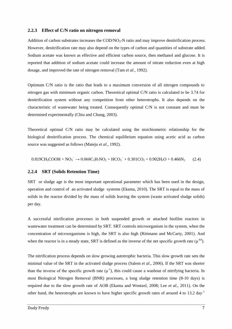
2.2.3 Effect of C/N ratio on nitrogen removal
Addition of carbon substrates increases the COD/NO3-N ratio and may improve denitrification process.
However, denitrification rate may also depend on the types of carbon and quantities of substrate added.
Sodium acetate was known as effective and efficient carbon source, then methanol and glucose. It is
reported that addition of sodium acetate could increase the amount of nitrate reduction even at high
dosage, and improved the rate of nitrogen removal (Tam et al., 1992).
Optimum C/N ratio is the ratio that leads to a maximum conversion of all nitrogen compounds to
nitrogen gas with minimum organic carbon. Theoretical optimal C/N ratio is calculated to be 3.74 for
denitrification system without any competition from other heterotrophs. It also depends on the
characteristic of wastewater being treated. Consequently optimal C/N is not constant and must be
determined experimentally (Chiu and Chung, 2003).
Theoretical optimal C/N ratio may be calculated using the stoichiometric relationship for the
biological denitrification process. The chemical equilibrium equation using acetic acid as carbon
source was suggested as follows (Mateju et al., 1992).
0.819CH3COOH + NO3− → 0.068C5H7NO2 + HCO3
− + 0.301CO2 + 0.902H2O + 0.466N2 (2.4)
2.2.4 SRT (Solids Retention Time)
SRT or sludge age is the most important operational parameter which has been used in the design,
operation and control of an activated sludge systems (Ekama, 2010). The SRT is equal to the mass of
solids in the reactor divided by the mass of solids leaving the system (waste activated sludge solids)
per day.
A successful nitrification processes in both suspended growth or attached biofilm reactors in
wastewater treatment can be determined by SRT. SRT controls microorganism in the system, when the
concentration of microorganisms is high, the SRT is also high (Rittmann and McCarty, 2001). And
when the reactor is in a steady state, SRT is defined as the inverse of the net specific growth rate (μ-kd
).
The nitrification process depends on slow growing autotrophic bacteria. This slow growth rate sets the
minimal value of the SRT in the activated sludge process (Salem et al., 2006). If the SRT was shorter
than the inverse of the specific growth rate (μ-1
), this could cause a washout of nitrifying bacteria. In
most Biological Nitrogen Removal (BNR) processes, a long sludge retention time (8-10 days) is
required due to the slow growth rate of AOB (Ekama and Wentzel, 2008; Lee et al., 2011). On the
other hand, the heterotrophs are known to have higher specific growth rates of around 4 to 13.2 day-1

8 MSc Thesis
than nitrifiers which have specific growth rates of only around 0.62 to 0.92 day-1
respectively (Okabe
et al., 2011).
It is reported that the nitrogen removal efficiency was higher when the SRT increased (Ekama and
Wentzel, 2008). Lee et al. (2008) studied the total nitrogen removal efficiency of an SBR. He
observed that the TN removal efficiency could be obtained up to 66.9% at SRT 16.2 days. However as
the SRT increased, the denitrification rate per mixed liquor suspended solids (MLSS) during the first
anoxic period decreased significantly (Lee et al., 2008). Moreover, another study identified that the
long SRT had bettered the process. It was found that at the SRT between 10.3 to 34.3 days could
lessened the unfavourable effect of low temperatures and stabilized the nitrification process
(Komorowska-Kaufman et al., 2006).
The effect of SRT on flocs sludge characteristics in SBR was studied by Liaou, et al. (2006). It
indicated that floc size was relatively stable and not subject to influence by SRT or organic loading in
SBR. This study also advised that SRT should be larger than the critical SRT (9–12 days) to maintain
a relatively stable microbial community for effective biomass flocculation and separation (Liao et al.,
2006)
In a study of algal-bacterial system in SBR, biomass productivity was generally increased as retention
times decreased (Valigore et al., 2012). And longer SRT enhanced biomass settleability while shorter
Hydraulic Retention Time (HRT) enhanced productivity except when washout occurred (Valigore et
al., 2012)
2.2.5 Sequential Batch Reactor (SBR)
Sequential batch reactor is a modification of activated sludge process. Whereas successfully used to
treat municipal and industrial wastewater (Mahvi, 2008). The difference is that the SBR performs
equalization, biological treatment, and secondary clarification in a single tank/reactor using a timed
control sequence.
In SBR, treatment of wastewater is carried out in various consecutive phases namely filling, reaction,
settling, and decant (as shown in Figure 2.1). The removal of nitrogen can be achieved by alternating
aerobic and anoxic periods during the reaction (Rodríguez, Pino, et al., 2011). The duration of each
cycle and the number of stages of operation depends on the type of wastewater to be treated
(Rodríguez, Ramírez, et al., 2011). The advantages of operation in SBR are single-tank configuration,
small foot print, easily expandable, simple operation and low capital costs (Mahvi, 2008).

Dudy Fredy 9
Figure 2.1:Typical cycles in Sequential Batch Reactor
Source: (Mahvi, 2008)
Many studies have been done with the different operational sequences as shown in Table 2.3, and
generally the objectives were to optimize nitrogen removal.
Table 2.3: Different operational sequences of SBR operation
Operational mode Operational overview Reference
Intermittenly aerated
SBR to treat high
phenol concentration
(Singh and
Srivastava,
2011)
Automatically
controlled SBR to
enhance nitrogen
removal, step-feed
strategy, without
external carbon
source
(Puig et al.,
2005)
Automatically
controlled SBR to
enhance nitrogen
removal, step-feed
strategy, with external
carbon source
Guo et al.
(2007)

10 MSc Thesis
Operational mode Operational overview Reference
Automaticallay
controlled (real time)
SBR to remove
nitrogen via nitrite,
external carbon
source
(Wu et al.,
2011)
A pilot scale SBR to
treat high amount of
organic matter and a
high amount of
ammonium
(Rodríguez,
Ramírez, et al.,
2011)
Source :(Windraswara, 2013)
Irvine and Bush (1979) reported that SBR is an effective biological treatment method for removing
organic matter and nutrients. It could be done by distributing the influent injection and aeration
periods variably and appropriately. In particular, a higher efficiency of denitrification can be achieved
in the SBR method by varying the proportional distribution of the durations of the anoxic and aerobic
periods during one-cycle operation. Lee et al., (2007) indicated that increasing the duration of the
anoxic (II) period, which is conducive to denitrification, increases the efficiency of nitrogen removal
by denitrification.
2.3 Algal-bacterial consortium for wastewater treatment
The application of algal–bacterial biomass for wastewater treatment now is becoming more interesting.
It presents lower energy consumption via photosynthetic aeration (Muñoz et al., 2004; Safonova et al.,
2004; Muñoz and Guieysse, 2006), and offers the potential use as an alternative energy source (biofuel
or biogas) from its biomass. Furthermore the algal based system may also contribute to CO2 mitigation
(Muñoz and Guieysse, 2006; Subashchandrabose et al., 2011).
The interactions of microalgae and ordinary heterotrophic (OHOs) bacteria in wastewater treatment
process can be a symbiotic relationship. Microalgae provide the necessary O2 for heterotropic bacteria
to biodegrade organic pollutants, and the CO2 released from bacterial respiration is used for
photosynthesis. As autotrophic nitrifiers and hetereotrophic denitrifers are also present in the system,
the interactions between microorganisms become more complex, as shown in Figure 2.2.

Dudy Fredy 11
Figure 2.2:Interaction between algae and bacteria in wastewater treatment process
Moreover, microalgae and bacteria do not limit their interactions to a simple CO2-O2 interchange.
Microalgae may increase bacterial activity by releasing extracellular (Wolfaardt et al., 1994). While,
De-Bashan et al. (2002) reported that the presence of growth promoting bacteria Azospirillum
brasilense enhanced ammonium and phosphorous removal by C. vulgaris (de-Bashan et al., 2002).
However microalgae may also have an unfavorable effect on bacterial activity by increasing the pH,
the DO (Dissolved Oxygen) concentration, or the temperature of the cultivation broth, or by excreting
inhibitory metabolites (Oswald, 2003; Schumacher et al., 2003). Or even the other way around
bacteria may inhibit microalgae by producing algicidal extracellular metabolites (Fukami et al., 1997).
Nevertheless, treatment of wastewater using the interaction of algal-bacterial was developed. W.J.
Oswald in the year 1950s introduced such kind technology for sewage treatment (Oswald and Gotaas,
1957). Since then, many improvements have led to the use of algal-bacterial consortium in facultative
ponds, high rate algal ponds (HRAP), and closed photo-bioreactors (Babu et al., 2010; Park et al.,
2011; Subashchandrabose et al., 2011; Craggs et al., 2012). Table 2.4 summarizes various studies that
reported results on nutrient removal by algal-bacterial consortium to treat wastewater.
ALGAE
OHOs
NITRIFIERS
DENITRIFIERS
LIGHT
Wastewater BIOMASS
CO2
N
CO2
N
NO3
Organics
O2
Reclaimed Water
CO2


12
M
Sc T
hesis
Table 2.4: Algal-bacterial consortium for nutrient removal from wastewater
Cyanobacterium/microalga Bacterium Source of wastewater Nutrients
Removal
Efficiency
(%)
Initial conc
(mg/l) Reactor used
Spirulina platensis Sulfate-reducing bacteria Tannery effluent Sulfate 80 2000 High rate algal pond (HRAP)
Chlorella vulgaris Azospirillum brasilense Synthetic wastewater Ammonia 91 21 Chemostat
C. vulgaris Wastewater bacteria Pretreated sewage DOC 93 230 Photobioreactor pilot-scale
nitrogen 15 78
C. vulgaris Alcaligenes sp. Coke factory wastewater NH4+ 45 500 Continuous photobioreactor
with sludge recirculation phenol 100 325
C. vulgaris A. brasilense Synthetic wastewater Phosphorous 31 50 Inverted conical glass bioreactor
nitrogen 22 50
Chlorella sorokiniana Mixed bacterial culture
from an AS
Swine wastewater Phosphorous 86 15 Tubular biofilm photobioreactor
nitrogen 99 180
C. sorokiniana Activated sludge bacteria Pretreated piggery wastewater TOC 86 645 Glass bottle
nitrogen 87 373
C. sorokiniana
Activated sludge
consortium Pretreated piggery slurry TOC 9 to 61 1247
Tubular biofilm photo
bioreactor
nitrogen 94-100 656
Phosphorous 70-90 117
C. sorokiniana Activated sludge bacteria Piggery wastewater TOC 47 550 Jacketed glass tank
photobioreactor phosphorous 54 19
NH4+ 21 350
Euglena viridis Activated sludge bacteria Piggery wastewater TOC 51 450 Jacketed glass tank
photobioreactor phosphorous 53 19
NH4+ 34 320
Abbreviations: DOC=dissolved oxygen concentration; TOC=total organic carbon
Source: (Subashchandrabose et al., 2011)

Dudy Fredy 13
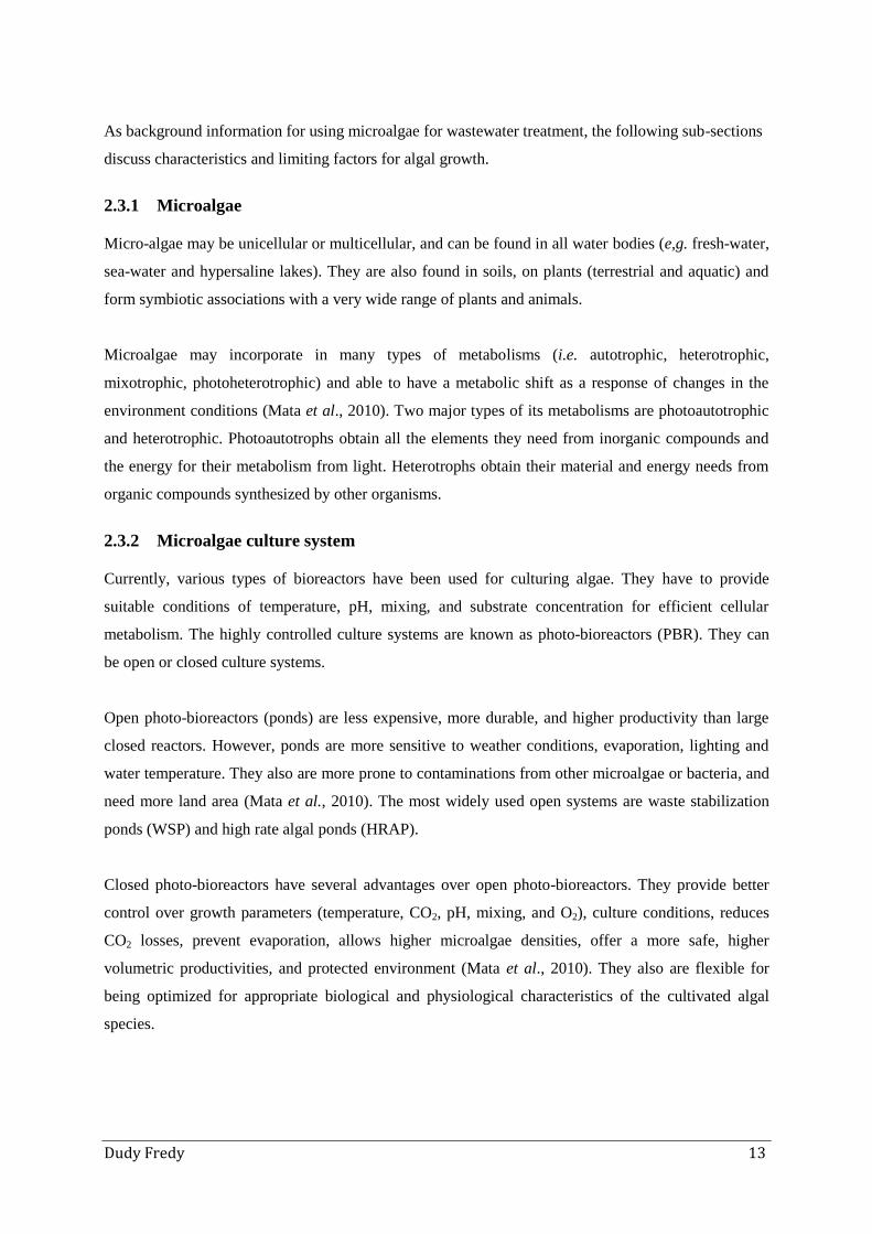
As background information for using microalgae for wastewater treatment, the following sub-sections
discuss characteristics and limiting factors for algal growth.
2.3.1 Microalgae
Micro-algae may be unicellular or multicellular, and can be found in all water bodies (e,g. fresh-water,
sea-water and hypersaline lakes). They are also found in soils, on plants (terrestrial and aquatic) and
form symbiotic associations with a very wide range of plants and animals.
Microalgae may incorporate in many types of metabolisms (i.e. autotrophic, heterotrophic,
mixotrophic, photoheterotrophic) and able to have a metabolic shift as a response of changes in the
environment conditions (Mata et al., 2010). Two major types of its metabolisms are photoautotrophic
and heterotrophic. Photoautotrophs obtain all the elements they need from inorganic compounds and
the energy for their metabolism from light. Heterotrophs obtain their material and energy needs from
organic compounds synthesized by other organisms.
2.3.2 Microalgae culture system
Currently, various types of bioreactors have been used for culturing algae. They have to provide
suitable conditions of temperature, pH, mixing, and substrate concentration for efficient cellular
metabolism. The highly controlled culture systems are known as photo-bioreactors (PBR). They can
be open or closed culture systems.
Open photo-bioreactors (ponds) are less expensive, more durable, and higher productivity than large
closed reactors. However, ponds are more sensitive to weather conditions, evaporation, lighting and
water temperature. They also are more prone to contaminations from other microalgae or bacteria, and
need more land area (Mata et al., 2010). The most widely used open systems are waste stabilization
ponds (WSP) and high rate algal ponds (HRAP).
Closed photo-bioreactors have several advantages over open photo-bioreactors. They provide better
control over growth parameters (temperature, CO2, pH, mixing, and O2), culture conditions, reduces
CO2 losses, prevent evaporation, allows higher microalgae densities, offer a more safe, higher
volumetric productivities, and protected environment (Mata et al., 2010). They also are flexible for
being optimized for appropriate biological and physiological characteristics of the cultivated algal
species.

14 MSc Thesis
2.3.3 Influence of environmental parameters on algal growth
The growth rate of microalgae is influenced by physical (e.g. light and temperature), chemical (e.g.
availability of nutrients, carbon dioxide, pH), biological factors (e.g. competition between species,
grazing by animals, virus infections) and operational factors (e.g. bioreactor design, mixing and
dilution rate) (Larsdotter, 2006). Some of the most important parameters are described in below sub-
sections.
2.3.3.1 Light
Microalgae are phototrophs, they obtain energy from light. The light energy is converted to chemical
energy in the photosynthesis, but large parts are lost as heat. Oswald (1988) reported that in outdoor
ponds, more than 90% of the total incident solar energy is converted into heat and less than 10% into
chemical energy. Fontes (1987) reported a conversion efficiency of sunlight energy into chemical
energy of only 2% (Larsdotter, 2006).
The relationship between light intensity and photoautotrophic cell growth or various cell activities is
rather complex. Algal activity increases with light intensity up to 200–400 µE/m2.s (Muñoz and
Guieysse, 2006), while insufficient light lowers the growth rate. Anexcess light may lead to
photoinhibiton (Hsieh and Wu, 2009). Photoinhibition has therefore been observed at noon of a sunny
day when irradiance can reach more than 4000 µE/m2.s (Fuentes et al., 1999; Carvalho et al., 2011). A
typical relation between light intensity and photoautotrophic growth is shown in Figure 2.3.
Figure 2.3: Relation between light intensity on photoautotrophic growth of photosynthetic cells
Source: (Ogbonna and Tanaka, 2000)

Dudy Fredy 15
Absence of light or low light intensity can also lower photosynthesis efficiency, and it will leads to
anaerobic conditions in the reactor (Muñoz and Guieysse, 2006). Some algae are able to grow in the
dark using simple organic compounds as energy and carbon source (heterotrophic) (Perez-Garcia et al.,
2010), and their cells metabolize their components to obtain maintenance energy, thus leading to a
decrease in cell weight (Ogbonna and Tanaka, 2000).
2.3.3.2 Temperature
The growth rate of algae increases with the increased of temperature. As cited by Park et al., (2011),
Soeder et al., (1985) observed that the optimal temperature for maximum algal growth rate (sufficient
nutrient and light conditions) varies between algal species. The optimal temperature for many algae is
between 28 and 35°C. While Harris (1978) reported that optimal temperature also varies when nutrient
or light conditions are limited. The algae growth often declines when encounter to a sudden
temperature change (Park et al., 2011).
Temperature is also well connected with light intensity. As cited in (Muñoz and Guieysse, 2006),
Abeliovich (1986) reported that excessive temperature can happen at high light intensities and high
biomass concentrations, from the fact that algae convert a large fraction of the sunlight into heat.
2.3.3.3 Nutrients
Algae nutritional requirements can be classified into macronutrients (i.e. those required at g/L
concentrations) and micronutrients (i.e. those required at mg/L or μg/L concentrations). The primary
essential elements for the growth of algae are carbon, nitrogen and phosphorus. Algae also need some
trace elements including calcium, iron, silica, magnesium, manganese, potassium, copper, sulfur,
cobalt and zinc which are also essential but rarely affect its growth in wastewater treatment
(Christenson and Sims, 2011).
Ammonium and nitrate are the most commonly inorganic nitrogen sources in algal media. Some of the
prokaryotic algae, the blue-green algae (cyanobacteria), can also fix atmospheric N2. The pH of the
medium may decreased when ammonium is used as the only nitrogen source. In dense cultures and
high temperatures, the lower pH may result into a rapid decline in growth or even death of the culture.
It is also reported that high concentrations (more than one mM) ammonium may inhibit growth,
especially at high temperatures (Borowitzka, n.d.).
If both ammonium and nitrate are supplied the cultures generally do not take up the nitrate until the
ammonium has been used up. This is because ammonium is the end product of nitrate reduction,

16 MSc Thesis
therefore it may cause feedback-inhibition and repression of the nitrate uptake and reduction system
(Borowitzka, n.d.)
Phosphorous is another major nutrient for algae, as an inorganic form of phosphate (H2PO4- and
HPO42-
). The take up is started by hydrolysis with the action of phosphoesterase or phosphatase
enzymes The amount of inorganic phosphorus required by algae varies among algae species. The
tolerance amount is normally around 50 μg/L – 20 mg/L (Becker, 1994).
2.3.3.4 pH
pH may have a great effect on the microalgae growth rate and species composition. For example, it
was found that the optimal productivity of Anabaena variabilis (cyanobacterium) was achieved at pH
8.2 – 8.4 and decreased slightly at pH 7.4 – 7.8, while at pH 9.7 – 9.9 the cell could not survive
(Larsdotter, 2006).
Photosynthetic assimilation (CO2 uptake by algae) may also increase pH in the medium. The increase
of pH can reach 11 or more if CO2 is limiting and bicarbonate is used as a carbon source (Larsdotter,
2006).
Nitrogen assimilation by the algae also affects pH. Assimilation of nitrate ions tend to raise the pH,
but if ammonia is used as nitrogen source, the pH of the medium may decrease to as low as 3 (Becker,
1994). At high pH (above 9) free ammonia will begin to dominate over ammonium. High
concentrations of ammonia may inhibit algal growth, and this toxicity is intensified at higher
temperatures which may freely diffuse over membranes into the cells (Larsdotter, 2006; Markou and
Georgakakis, 2011).
2.3.3.5 Dissolved Oxygen (DO)
The process of photosynthesis is the main source of DO in outdoor ponds. The amount of DO
concentration depends on the growth rate of algae, light intensity and temperature; it reaches a
maximum value during noon and then decreases as light and temperature decrease. A study using
P.carterae showed that the maximum concentration of O2 during the day was directly related to light
irradiance. The highest photosynthetic rate was obtained in high light (1,900 μmol photons/m2.s) and
at low oxygen concentration (6–10 mg O2/L). However, high concentrations of oxygen (26–32 mg
O2/L) at both low and high irradiances, strongly increase the degree of inhibition of photosynthesis
(Moheimani and Borowitzka, 2007).
Dudy Fredy 17
2.3.3.6 Carbon
Microalgae obtain energy through photosynthesis. As indicated in the photosynthetic equation 2.4,
solar energy is converted into chemical energy and this energy is then used to assimilate inorganic
carbon (CO2) to produce sugars and oxygen as a by-product.
6 H2O + 6 CO2 + light 6 C6H12O6 + 6 O2 (2.4)
Inorganic (CO2 and HCO3-) and organic carbon are utilized by algae in the ponds as well as in algal
culture systems. The organic carbon sources can be assimilated either chemo- or photo-
heterotrophically (Larsdotter, 2006). In the first case, the organic substrate is used both as the source
of energy (through respiration) and as carbon source, while in the second case, light is the energy
source. In several algal species e.g. Chlorella and Scenedesmus, the mode of carbon nutrition can be
shifted from autotrophy to heterotrophy when the carbon source is changed (Becker, 1994).
The amount of CO2 dissolved in water varies with pH, where an addition of CO2 results in a decreased
pH. At higher pH values, for example at pH greater than 9, most of the inorganic carbon is in form of
carbonate (CO3 2–
) which cannot be assimilated by the algae. The decreased availability of CO2 may
act as a limiting factor on the algal growth, however his effect is not often evident. Aeration is one of
few ways in providing carbon dioxide for algae growth (Larsdotter, 2006).
A study observed in Chlorella sp. cultivation in photo-bioreactors showed that 2% aeration of CO2
increased the total biomass productivity (Chiu et al., 2008). The CO2 demand for microalgae can also
be calculated based on its stoichiometric requirement because 1 g biomass requires 1.85 g CO2. For
example, if the growth rate of biomass is 1 g/(g.d) at biomass concentration 1 g/L, then the carbon
transfer rate needed would be 1.85 g/(L.d) (Posten, 2009).
2.4 Effect of dark periode on nitrogen removal
Irradiance or light is one of the major factors, which control microalgae productivity. Absence of light
can cause a reduction of photosynthesis activity, which normally leads to the occurrence of anaerobic
conditions in the reactor. This condition is assumed to be favored for denitrification process. In
activated sludge system, denitrification has been observed to begin when DO concentration in the
flocs drops below 0.6 mg/L (Schramm et al., 1999).
On the other hand, there are a number of microalgae that can grow mixotrophically. Mixotrophic
growth regime is a variant of the heterotrophic growth regime, where CO2 and organic carbon are

18 MSc Thesis
simultaneously assimilated and both respiratory and photosynthetic metabolism operate concurrently
(Perez-Garcia et al., 2011). In the absence of light, there may be a competition between microalgae
and bacteria for an organic carbon source, which may result in a negative effect on the denitrification
process.

Dudy Fredy 19
3 Objectives
3.1 General objective
To optimize nitrogen removal in a Sequential Batch Photo-bioreactor fed with artificial UASB effluent
by variations in operational conditions.
3.2 Specific objectives
1. To study the effects of different operational sequences in an SBR cycle on the nitrification and
denitrification capacity of microalgae and bacteria consortium in a Sequential Batch Photo-
bioreactor.
2. To study the effect of SRT on the nitrification and denitrification capacity of microalgae and
bacteria consortium in a Sequential Batch Photo-bioreactor.

20 MSc Thesis
Dudy Fredy 21
4 Material and Methods
The research was carried out in UNESCO-IHE laboratory in Delft, the Netherlands and it was a
continuation of previous MSc thesis research by UNESCO-IHE student Rudatin Windaswara
(Windraswara, 2013). The photo-bioreactors was operated in the SBR mode, controlled by a
bioconsole system, and connected to a data logger for DO concentration and pH measurement. The
work included operating the system, preparing artifical wastewater, sampling and analyzing nitrogen
compounds, chlorophyll-a, VSS/TSS, COD, and light absorption. Nitrogen conversion rates are
determined and nitrogen mass balances are developed.
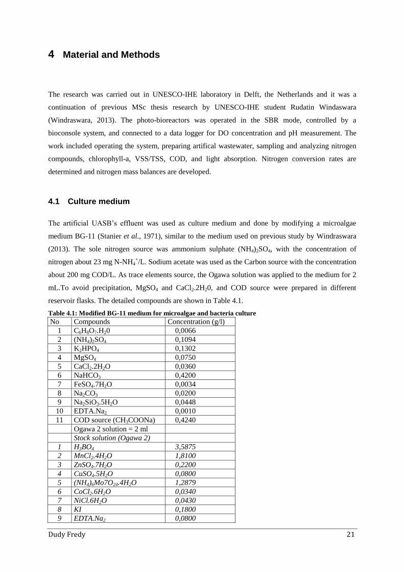
4.1 Culture medium
The artificial UASB’s effluent was used as culture medium and done by modifying a microalgae
medium BG-11 (Stanier et al., 1971), similar to the medium used on previous study by Windraswara
(2013). The sole nitrogen source was ammonium sulphate (NH4)2SO4, with the concentration of
nitrogen about 23 mg N-NH4+/L. Sodium acetate was used as the Carbon source with the concentration
about 200 mg COD/L. As trace elements source, the Ogawa solution was applied to the medium for 2
mL.To avoid precipitation, MgSO4 and CaCl2.2H20, and COD source were prepared in different
reservoir flasks. The detailed compounds are shown in Table 4.1.
Table 4.1: Modified BG-11 medium for microalgae and bacteria culture
No Compounds Concentration (g/l) 1 C6H8O7.H20 0,0066 2 (NH4)2SO4 0,1094 3 K2HPO4 0,1302 4 MgSO4 0,0750 5 CaCl2.2H2O 0,0360 6 NaHCO3 0,4200 7 FeSO4.7H2O 0,0034 8 Na2CO3 0,0200 9 Na2SiO3.5H2O 0,0448
10 EDTA.Na2 0,0010 11 COD source (CH3COONa) 0,4240 Ogawa 2 solution = 2 ml Stock solution (Ogawa 2) 1 H3BO4 3,5875 2 MnCl2.4H2O 1,8100 3 ZnSO4.7H2O 0,2200 4 CuSO4.5H2O 0,0800 5 (NH4)6Mo7O24.4H2O 1,2879 6 CoCl2.6H2O 0,0340 7 NiCl.6H2O 0,0430 8 KI 0,1800 9 EDTA.Na2 0,0800

22 MSc Thesis
4.2 Microalgae-bacteria consortium
Biomass culture was consisted of algae species Scenedesmus quadricauda, Chlorella sp, Anabaena
variabilis, Chlorococcus sp, and Spirulina sp, enriched with wild algae species from a canal in Delft,
the Netherlands. Nitrifying and denitrifying bacteria population were taken from fresh sludge of
Harnaschpolder Wastewater Treatment Plant (WWTP), Delft, the Netherlands.
4.3 Reactor set up and experimental design
The experiment was conducted in 1-L cylindrical jacketed and transparent glass reactor. The
temperature and pH during React phase was kept at 28oC and 7.5, respectively. Four sets of standing
lamps (Phillips, the Netherlands) were installed at four sides of the reactor (average light intensity on
the surface of reactor’s wall of 25.9 µmol/m2s). Mixing was maintained at 200 rpm during Fill and
React phases, and DO concentration and pH were measured and recorded using the DO probe from
Bio-console Applikon, the Netherlands. The schematic diagram of reactor set-up is shown in Figure
4.1.
Figure 4.1: Schematic diagram of reactor set up
Source: (Karya et al., 2013)

Dudy Fredy 23
The reactor was operated as an open system of SBR, with two cycles per day (1 cycle in 12 hours).
The experimental variations were done in four periods. The first two periods were done in different
sequential operation and the other three periods were done in different SRT as described in Table 4.2.
Table 4.2: Experimental variations
Period Sequential operation in one cycle of SBR mode SRT
(days)
1
48
2
52
3
26
4
17
The more detailed operational setting of one cycle for each period is described in Table 3.3 and Table
3.4. Withdrawal of the effluent was 50% of the total reactor volume. The duration of each SBR phases
were controlled using a set of automatic controllers from Bio-Console Applikon, Holland.
Table 4.3: SBR operational setting at period 1
No Phase Time
(min) Set
pH Light Stirrer Remark
0 initialization 0 NA on
on
1 start 2 7.5
on
2 filling 1 8 7.5 400 ml of substrate
3 aerobic 1 440 7.5
4 pre anoxic 15 7.5
off
5 filling 2 2 7.5 100 ml of COD source
6 anoxic 73 7.5
7 aerobic 2 60 7.5
on
8 settling 105 NA
off
9 withdrawing 10 NA
10 iddle 5 NA
Total time 720
Influent
WithdrawFilling Aerobic 1 Anoxic Aerobic 2 Settling
Carbon source
Withdraw
Filling 1
Aerobic 1Anoxic 1 Aerobic 2 Settling
Influent and
Carbon source
Anoxic 2
Influent and
Carbon source
Filling 2

24 MSc Thesis
Table 4.4: SBR operational setting at period 2, 3 and 4
No Phase Time
(min) Set
pH Light Stirrer Remark
0 initialization 0 NA on
on
1 start 2 7.5
off
2 pre-anoxic 1 13 7.5
3 filling 1 4 7.5 200ml of substrate + 50
mL of COD
4 anoxic 1 26 7.5
5 aerobic 1 255 7.5 on
6 pre-anoxic 2 15 7,5
off
7 filling 2 4 7.5 200ml of substrate + 50
mL of COD
8 anoxic 2 26 7.5
9 aerobic 2 255 7.5
on
10 settling 115 NA
off
11 withdrawing 4 NA
12 iddle 1 NA
Total time 720
4.4 Sampling
The samples for daily influent nitrogenous and COD concentrations were taken from the influent
reservoirs at the beginning of the cycle. While the effluent samples were collected during the withdraw
phase at the end of the cycle. For light absorption, TSS/VSS and chlorophyll-a analysis, the samples
were collected after second filling phase completed. For all nitrogenous analysis, samples are filtered
directly after the collection using 0.45 μm filter, and then stored in the refrigerator (4oC) for the
analysis.
4.5 Analytical Methods
4.5.1 Ammonium nitrogen
Based on NEN 6472 method, ammonium nitrogen concentration was measured using the
spectrophotometer. Samples were filtered over a glass fiber (GF/C), pipetted into a 50 mL flask and
reacted with sodium salicylate reagents and dichloroisocyanurate reagents. A series of standards of
NH4Cl solutions were used from standard solution with known concentrations to develop a calibration
curve. By using the spectrophotometer, the absorbance of each standard sample and the samples were
measured at the wavelength of 655 against water with 1 cm cells between 1 to 3 hours. The results of

Dudy Fredy 25
these standards were plotted against their known concentrations to determine the mathematical
expression which further were used to determine the concentration of samples from the experiment.
4.5.2 Nitrite nitrogen
Nitrite nitrogen concentration was determined according to Standard Methods for examination of
water and wastewater from American Public Health Association (APHA, 1995). The analysis was
using the colorimetric procedure which employs two organic reagents, namely sulfanilamide and N-(1
Naphtyl)-ethylenediamine dihydrocloride. An amino group from sulfanilamide reacts with nitrite ion
as nitrous acid which resulted in a pinkish-red azo dye. A series of NO2- standards were used to
develop a calibration curve in each analysis of the samples. Diluted samples were mixed with 2 mL of
mixed reagents in 50 mL flasks after which the photometric measurement was conducted at the
wavelength of 543 nm against water with 1 cm cell (between 10 minutes to 2 hours).
4.5.3 Nitrate nitrogen
Ion chromatography method using Dionex ICS-1000 is used to determine nitrate nitrogen
concentration. Samples were filtered through 0.45 μm filters immediately after collection to prevent
the bacteria in the sample that may change the ionic concentrations. Dilution of samples by using de-
ionized water was needed to avoid high concentrations of nitrite nitrogen not greater than 10 mg/L.
For analysis, 5 mL of samples was placed in high density polyethylene containers and washed
thoroughly using de-ionized water.
4.5.4 Chlorophyll-a
Chlorophyll-a concentration was determined according to Dutch Standard NEN 6520. Samples were
filtered by using GF6 filter (0.45 μm porosity) and transferred to Schott GL 18 COD tubes. The
chlorophyll-a was extracted using 80% (v/v) ethanol. To achieve complete pigment extraction, brief
heating for about 5 minutes in a water bath at temperature of 75oC was conducted. To promote better
extraction, furthermore the tubes were shaken several times and cooled to room temperature. After
centrifugation, the supernatant was analyzed in spectrophotometer at a wavelength of 665nm against
80% ethanol. For turbidity correction, measurement at a wavelength of 750 was also carried out. After
obtaining the absorbance reading, 2 drops of 0.4 M HCl were added to each sample and (5 to 30)
minutes later the samples were re-measured at the same wavelengths. The following equation was
used to calculate the chlorophyll-a concentration:
Chl-a (μg/L) = 296 * V1 * En-Ea/(Vo * p) (4.1)

26 MSc Thesis
Where En=Ex-Eo is the corrected absorbance of the non-acidified extract, Ea=Exa-Eoa is the
corrected absorbance of the acidified extract, 296 is a correction factor on the specific absorption
coefficient of Chl-a, V1 is the volume of 80% ethanol in mL, Vo is the sample volume in L and p is
the cell thickness in mm.
4.5.5 Total suspended solid (TSS) and volatile suspended solid (VSS)
The determination of TSS and VSS involved of drying the samples at 105oC in an oven and
combustion at 520oC in a muffle furnace according to APHA (1995). Well mixed samples were
filtered using weighed GF/C filters which had been pre-heated for 2 hours at 520oC and stored in a
desiccator. Filtered sludge solids were placed in aluminum cups and left in the oven at 105oC for 2
hours then weighted. The dry weight (TSS) is calculated by substracting the dry weight (sample+filter)
from a clean weight (filter). Samples were put back in the cups, combusted at 520oC for 3 hours and
cooled in a desiccator before weighing. The difference in weight before and after combustion
represented the VSS (g/L).
4.5.6 Biomass Light Absorption
The well mixed of liquor sample from the reactor was consisted of biomass with certain chlorophyll-a
concentration. Its light absorption was determined by using a spectrophotometer in a 1 cm cuvette.
The initial light intensity was measured with an LI-COR LI-1400 quantum sensor. Repeating the
procedure with a cuvette blanked with medium, the biomass light aborption coefficient could be
determined by rearranging equation Beer-Lambert’s Law as:
ka =
(4.2)
where I is a light intensity at distance z, Io is the incident light intensity at the reactor, B is the biomass
concentration, and ka is the biomass light absorption coefficient.
4.6 Calculation
4.6.1 Solid Retention Time (SRT)
The actual SRT was determined based on formula in a study done by (Valigore et al., 2012). This
formula also considers the biomass concentration in wastage during discharge. The formula is shown
below:

Dudy Fredy 27
(4.3)
Where: Xr biomass concentration in the reactor (mg/L)
Xs biomass supernatant (mg/L)
Qw waste dischare flowrate (L/day)
Qs supernatant discharge flowrate (L/day)
4.6.2 Nitrogen balance
Nitrogen balance in the reactor was obtained from the overall nitrification equation by using the
stoichiometric link developed by Liu and Wang in their study (Liu and Wang, 2012). The equation
provides a more accurate stoichiometric link between nitrifier yield, ammonia consumption, and
oxygen uptake for both steps of the nitrification process. And also considers the amounts of ammonia
incorporated into the cells of ammonia oxidizers and nitrite oxidizers.The complete nitrification
equation is shown below:
NH4+ + 0.0298NH4
+ + 1.851O2 + 0.1192CO2 + 0.0298HCO3
-
0.0298C5H7O2N + NO3- + 0.9702 H2O (4.4)
Initial ammonium concentration
Initial ammonium concentration was obtained from the measurement of influent concentration in the
reservoir and multiplied it by dilution factor.
Ammonium uptake by nitrifiers (AOB and NOB)
Equation 4.4 shows that when 1 unit of ammonia is oxidized into nitrite then into nitrate, 0.0298 unit
of ammonia-nitrogen would be incorporated into nitrifiers.
Nitrified ammonium
The highest nitrate concentration in react phase (sum of aerobic 1 and aerobic 2 for period 2 to 4) has a
correlation with the ammonium nitrogen that had been oxidized (nitrified ammonium). The nitrified
ammonium was calculated from the Equation 4.4 which shows that 1 mg N-NO3- is formed from (1+
0.0298) mg N-NH4+.
Ammonium uptake by algae
Since the initial ammonium nitrogen concentration is higher than the amount that had been nitrified, it
means the difference was assumed as ammonium that had been uptaken by algae. And it can be
assumed that there was no NO3- uptake by algae.

28 MSc Thesis
4.6.3 Biomass composition
There are at least four different organisms that contributed to the total biomass in the reactor of algae-
bacteria consortia. Those four microorganisms namely are autotrophic nitrifiers, heterotrophic
denitrifiers, ordinary heterotrophic organisms (OHO) and algae itself. The calculations of biomass
production are described below:
Nitrifiers biomass production
Nitrifiers biomass production was obtained from Equation 4.4, where 1 mg N-NO3- produced 0.24 mg
of biomass (C5H7O2N).
Denitrifiers biomass production
The denitrifiers organisms biomass was calculated stoichiometrically based on nitrate formed during
the reaction phase. From the denitrification equation (Mateju et al., 1992) which used acetate as a
carbon source, 0.55 mg of biomass (C5H7O2N) is produced from 1 mg N-NO3- , as shown below:
0.819CH3COOH + NO3− → 0.068C5H7NO2 + HCO3
− + 0.301CO2 + 0.902H2O + 0.466N2 (4.5)
OHO biomass production
Ordinary heterotrophs biomass was obtained through the stoichiometry of acetate oxidation equation.
The biological reaction for acetate oxidation is adapted from Metcalf and Eddy (2003) (Henze, 2008),
by combining three different half reactions of cell synthesis, electron acceptor and electron donor. The
overall balanced equation is shown below:
0.125CH3COO- + 0.0295NH4
+ + 0.103O2→ 0.0295C5H7NO2 + 0.095HCO3
− + 0.007CO2 + 0.955H2O
(4.6)
Based on the measurement of influent and effluent of COD, and from COD requirement for
denitrification through Equation 4.5, the COD that had been used for acetate oxidation can be known.
Furthermore the OHO biomass production can be calculated.
Algae biomass production
The algae biomass production was calculated from the photosynthesis reaction (Mara, 2003) below:
106CO2 + 236H20 + 16NH4+ + HPO4
2- C106H181O45N16P + 118O2 + 171H2O +14H
+ (4.7)

Dudy Fredy 29
The biomass production was calculated stoichiometrically based on the amount of ammonium uptake
by algae as described in section 4.6.2.
4.6.4 Oxygen production by algae
The estimation of oxygen production by algae was developed from the oxygen mass balances in one
cycle of SBR operation. The oxygen concentration profile of one cycle operation was divided into
three phase, as illustrated in Figure 4.2.
Figure 4.2: DO concentrations profile partition in one cycle of SBR operation
Phase I
It started from the beginning of the cycle until the DO concentration reach near zero mg/L. It assumed
that the respiration by algae was negligible. In this phase, the oxygen mass balance is shown below:
(Cs-C) + ralg – rnit – rhet (4.8)
Phase II
It occurred when the DO concentration reach near zero mg/L. In this phase, the oxygen mass balance
is developed with assumed that the respiration by algae was negligible, and the organic material
oxidation had completely finished.
(Cs-C) + ralg – rnit = 0 (4.9)
0
2
4
6
8
10
12
14
16
18
20
0 1 2 3 4 5 6 7 8 9 10 11 12
DO
co
nce
ntr
atio
n (
mg/
L)
Time (h) phase I
phase II phase III
slope of phase III
slope of phase I

30 MSc Thesis
Phase III
It occurred when the DO concentration rose until the second filling time. In this phase, the oxygen
mass balance assumed that the respiration by algae was negligible, and the organic material oxidation
and nitrification has completed.
(Cs-C) + ralg (4.10)
Where:
C DO concentration (mg/L)
Cs Saturation DO concentration (mg/L)
KLa oxygen mass transfer coefficient (1/hour)
ralg rate of oxygen generation by algae through photosynthesis (mg/hour)
rnit rate of oxygen consumption for nitrification (mg/hour)
rhet rate of oxygen consumption for organic matter oxidation (mg/hour)
The calculation procedures are described as follows:
a. Equation 4.10 can be derived as follow:
ralg
where r = KLa*Cs + ralg
k = KLa
=> -(1/k)·ln(r - k·C) = t + a (a is constant of integration)
r - k·C = e^(-k·(t+a)), after using initial condition to evaluate a
C(t) = r/k - (r/k - C₀)·e^(-k·t)
C(t) = r/k - (1 - e^(-k·t)) + Co* e^(-k·t)
C(t) = A - (1 - e^(-B·t)) + Co* e^(-B·t) (4.11)
b. Determine A and B, through curve fitting of equation 4.11 with data of experiments. The
curve fitting was done with online software in http://zunzun.com/
c. Determine the ralg from the value of A and B
d. Solution of equation 4.9 and 4.8 were done in similar way.

Dudy Fredy 31
4.7 Statistical analysis
Statistical analyses were performed using free software R Studio, version 0.97.551. Normality of the
data and homogeneity of variances were determined prior to any statistical treatments with a Shapiro-
Wilk’s test and Q-Q plots, respectively. And the normal distribution and homogeneity of variances
were not observed. The significant differences between mean values were analysed by Mann–Whitney
U-test, for period 1 and 2. The analysis was followed by Kruskal–Wallis H-test and a Tukey’s post
hoc test to see the significant differences between mean values of period 2, 3, and 4. Moreover, all
means were given as mean with standard deviation (number of measurements).
4.8 Batch experiment
To have a better understanding on nitrate uptake by algae in the reactor, batch experiment was
conducted.The same biomass culture and medium was used for the batch experiment. In the medium
the only Nitrogen source was supplied from NaNO3. Of each flask, 50 mL of the above culture was
grown in 200 mL of modified BG-11 medium in duplicate to gain three treatments of 0, 9, and 18
mg/L N-NO3-. The flasks were placed on a shaker with 140 rpm at room temperature. The lamp was
positioned above the shaker with 60 µmol m-2
s-1
photon. To avoid denitrification process occurred,
the light was always turned on for a period 24 hours per day. N-NO3- concentrations were measured
daily. After the entire N-NO3- was diminished in the flasks, refill of N-NO3
- was done to observe the
NO3- uptake performance.

32 MSc Thesis

Dudy Fredy 33
5 Results
5.1 Nitrogen removal
5.1.1 Daily nitrogenous concentration
The daily nitrogenous concentration profile for all periods is shown in Figure 5.1. Nitrification was
achieved completely without external aeration. A high concentration of nitrate in the effluent was
observed at the end of period 1 and within period 2. It was caused by insufficient COD source for
denitrification process, due to high algae growth in period 1 and COD supply failure in period 2. The
explanation of why COD could be the cause is discussed in section 6.1.
Figure 5.1: Daily nitrogenous concentration
The ammonium and total nitrogen removal efficiency is shown in Table 5.1. In general, the removal
efficiency for ammonium was 100% and for total nitrogen was 90%. As mentioned before due to
insufficient COD in the reactor, the nitrogen removal efficiency in period 2 was low 68%. However
there was no significant difference of nitrogen removal efficiency between all periods (P>0.05).
Table 5.1: Nitrogen removal efficiency
0.0
5.0
10.0
15.0
20.0
25.0
30.0
0 10 20 30 40 50 60 70 80 90 100 110 120 130 140 150 160 170
Nit
roge
no
us
con
cen
trat
ion
(m
g/L)
Days
Inf N-NH4 Eff N-NH4 Eff N-NO2 Eff N-NO3
Period Ammonium Removal
Efficiency (%) Total Nitrogen Removal
Efficiency (%)
Avg Std Dev Avg Std Dev 1 100 0.1 92.7 21.2
2 100 0.0 68.4 24.7
3 99.9 0.4 89.5 1.5
4 99.6 0.9 90.7 6.1
Period 1 Period 2 Period 3 Period 4

34 MSc Thesis
5.1.2 Ammonium conversion rate
A typical nitrogeneous concentration profile in one cycle of operation in the SBR system for period 2
is shown in Figure 5.2. From the linear part of ammonium conversion curves, conversion rate constant
in two different aerobic phases of the SBR operation were calculated. These rates were calculated
from the slope (ka and kb) where ka denotes ammonium conversion rate constant in first aerobic phase
and kb denotes ammonium conversion rate constant in the second aerobic phase.
Figure 5.2: Ammonium conversion in one cycle of SBR operation in period 2 day 89
The ammonium conversion rates for all periods are summarized in Table 5.2. The statistical tests were
done to see the differences of specific ammonium rate between each period. A significant difference
between the specific ammonium conversion rate of period 1 and period 2 could be demonstrated
(W=24, P<0.05).
Table 5.2: Summary of ammonium conversion rate in different period
Period Day Rate of ammonium conversion
(mgN-NH4/L.h) VSS
Rate of ammonium conversion (mgN-NH4/gVSS.h)
ka kb average k Std Dev g/L ka kb average k Std Dev
1
4 -2.5
-2.8 0.4
1.1 -2.3
-2.4 0.2 9 -2.7 1.1 -2.5
12 -3.2 1.3 -2.6 16 -2.7 1.3 -2.1
2 68 -3.0 -2.9
-2.9a 0.5 2.5 -1.2 -1.2
-1.1a 0.1 75 -3.3 -3.4 3.0 -1.1 -1.1 89 -2.7 -2.4 2.4 -1.1 -1.0
3
110 -2.0 -1.7
-2.1b 0.3
1.1 -1.9 -1.6
-2.2a 0.9 117 -2.6 -2.1 1.3 -2.1 -1.6 123 -2.3 -1.6 0.5 -4.5 -3.1 131 -2.3 -1.9 1.4 -1.6 -1.4 138 -2.2 -1.9 1.0 -2.2 -2.0
4 151 -2.2 -1.9
-2.1b 0.3 0.3 -7.7 -6.7
-4.7b 3.0 165 -2.5 -1.7 1.0 -2.5 -1.7
Note: Different superscripts denote significant differences between periods not sharing the same superscript.
Identical superscripts denote no significant difference. Values on period 1 was not included due to different
variation
0
1
2
3
4
5
6
7
8
0 2 4 6 8 10 12
Co
nce
ntr
atio
n (
mg/
L)
Hours
N-NH4
N-NO2
N-NO3
ka kb

Dudy Fredy 35
The specific ammonium conversion rate in period 1 was 2.4±0.2 mg/gVSS.h and then decreased in
period 2 to 1.1±0.1 mg/gVSS.h. The specific ammonium conversion rate of period 3 (2.2±0.9
mg/gVSS.h) seemed higher than period 2 (1.1±0.1 mg/gVSS.h), but the difference was not significant
(P>0.05).
5.2 Nitrogen balance
Table 5.3demonstrates nitrogen balance per cycle in different periods after the ammonium was
completely converted. The nitrified ammonium and the ammonium uptake by nitrifiers were
calculated stoichiometrically by using Equation 4.4. The calculation is based on the amount of nitrate
that was formed in the system during react (aerobic) phase. The ammonium uptake by algae was
calculated from the difference between initial concentrations and the uptake by the nitrifiers.
Table 5.3: Nitrogen balance based on one cycle operation in SBR
Period Day
Initial N-NH4+
concentration (mg/d)
N-NO3-
formed (mg/d)
Daily nitrified N-NH4+ (mg/d)
N-NH4+ uptake by nitrifiers (mg/d)
N-NH4+ uptake by algae (mg/d)
a b c % d avg StdDev % e avg StdDev %
1
4 18.8 14.6 15.0
77
0.4
0.5 0.0 2
3.8
4.8 1.1 23 9 21.2 14.8 15.2 0.4 6.0
12 20.2 15.8 16.3 0.5 3.9 16 21.8 15.8 16.3 0.5 5.5
2 68 27.2 9.5 9.8
48 0.3
0.4 0.1 1 17.4
14.1 5.5 52 75 28.4 11.0 11.3 0.3 17.1 89 24.0 15.7 16.2 0.5 7.8
3
109 26.94 11.3 11.6
41
0.3
0.3 0.0 1
15.4
16.6 1.3 59 117 28.07 11.3 11.6 0.3 16.4 123 27.05 10.7 11.0 0.3 16.0 131 30.40 11.3 11.6 0.3 18.8 138 28.20 11.3 11.7 0.3 16.5
4 151 24.68 11.9 12.3
59 0.4
0.4 0.1 2 12.4
10.2 3.2 41 165 24.72 16.3 16.8 0.5 7.9
Assumption: - no NO3 uptake by algae - no denitrification was occured
Note:
a calculated from measured influent concentration and dilution factor
b taken from the highest concentration in one cycle
c and d are calculated stoichiometrically from Equation 4.4 e = a-c
From Table 5.3, it shows that ammonium uptake by algae is increasing from 4.8±1.1 mg/d in period 1
up to 16.6±1.3 mg/d in period 3, with the assumption that there was no nitrate uptake by algae. On the
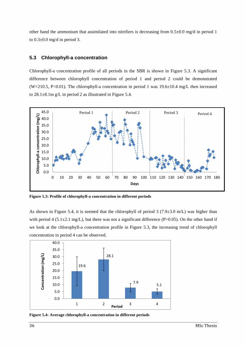
36 MSc Thesis
other hand the ammonium that assimilated into nitrifiers is decreasing from 0.5±0.0 mg/d in period 1
to 0.3±0.0 mg/d in period 3.
5.3 Chlorophyll-a concentration
Chlorophyll-a concentration profile of all periods in the SBR is shown in Figure 5.3. A significant
difference between chlorophyll concentration of period 1 and period 2 could be demonstrated
(W=210.5, P<0.01). The chlorophyll-a concentration in period 1 was 19.6±10.4 mg/L then increased
to 28.1±8.1m g/L in period 2 as illustrated in Figure 5.4.
Figure 5.3: Profile of chlorophyll-a concentration in different periods
As shown in Figure 5.4, it is seemed that the chlorophyll of period 3 (7.9±3.0 m/L) was higher than
with period 4 (5.1±2.1 mg/L), but there was not a significant difference (P>0.05). On the other hand if
we look at the chlorophyll-a concentration profile in Figure 5.3, the increasing trend of chlorophyll
concentration in period 4 can be observed.
Figure 5.4: Average chlorophyll-a concentration in different periods
0.0
5.0
10.0
15.0
20.0
25.0
30.0
35.0
40.0
45.0
0 10 20 30 40 50 60 70 80 90 100 110 120 130 140 150 160 170 180
Ch
loro
ph
yll-
a co
nce
ntr
atio
n (
mg/
L)
Days
19.6
28.1
7.9 5.1
0.0
5.0
10.0
15.0
20.0
25.0
30.0
35.0
40.0
1 2 3 4
Co
nce
ntr
atio
n (
mg/
L)
Period
Period 1 Period 2 Period 3 Period 4

Dudy Fredy 37
5.4 Suspended solids concentration
TSS and VSS concentration profile of all periods in the SBR are shown in Figure 5.5. The statistical
tests were done to see the differences of VSS average between each period. A significant difference
between VSS of period 1 and period 2 could be demonstrated (W=228.5, P<0.001). The VSS in period
1 was 1.7±0.7 g/L then increased to2.3±0.6 g/L in period 2 as illustrated in Figure 5.5
Figure 5.5: Profile of SS concentration in different periods
The VSS of period 3 (1.0±0.3 m/L) was not significantly different with period 4 (1.0±0.5 m/L)
(P>0.05). However if we look the biomass productivity from Figure 5.6, we can see that in period 4
the productivity is higher than in period 3.
Figure 5.6: Average SS concentration in different periods
0.00
0.50
1.00
1.50
2.00
2.50
3.00
3.50
4.00
4.50
0 10 20 30 40 50 60 70 80 90 100 110 120 130 140 150 160 170 180
SS c
on
cen
trat
ion
(g/
L)
Days TSS VSS
Biomass Productivity
avg Std dev avg Std dev (g/L.d) avg Std dev
1 2.6 0.9 1.7 0.7 0.035 0.65 0.11
2 2.9 0.8 2.3 0.6 0.045 0.82 0.03
3 1.1 0.4 1.0 0.3 0.037 0.90 0.04
4 1.1 0.6 1.0 0.5 0.053 0.91 0.03
PeriodTSS (g/L) VSS (g/L) VSS/TSS
0.0
1.0
2.0
3.0
4.0
1 2 3 4
SS C
on
cen
trat
ipn
(g/
L)
Period
TSS VSS
Period 2 Period 1 Period 3 Period 4

38 MSc Thesis
5.5 Light absorption
The light intensity was measured at the 12 points outer side of the reactor wall, and the average light
intensity was 25.9 µmol/s.m2, as shown in Figure 5.7a. The estimation of light penetration in the
reactor was developed using the Lambert-Beer Law. This is a basis for measuring the amount of light
absorption by the biomass inside the reactor. For simplification, a rectangular shape of reactor can be
assumed as its side view with radius 0.075 m (Figure 5.7b).
The light penetration into the reactor for each period can be seen in Figure 5.8. It can be seen that for
period 1 the light could only penetrate up to 1 cm from the outer wall, while in period 2, 3 and 4 the
light can penetrate up to 2 cm, 4 cm, and centre of the reactor respectively.
Figure 5.7: Light intensity measurement points (a) and a simplified side view of the reactor (b)
Figure 5.8: Estimated light penetration inside reactor
REACTOR
Lamp
D
Lamp
C
Lamp
A
Lamp
B
14.5 cm14.
5 cm
16.0 cm16.0
cm
A
E
C
D
B
F
G
H
I
J
K
L
0.0
4.0
8.0
12.0
16.0
20.0
24.0
28.0
0 0.01 0.02 0.03 0.04 0.05 0.06 0.07 0.08 Ligh
t In
ten
sity
( µ
mo
l/s.
m2
)
Reactor radius (m)
Period 1 Period 2 Period 3 Period 4
LAMP D
LAMP B
LAMP C
LAMP A
r=0.075 m
REACTOR
a b

Dudy Fredy 39
5.6 Biomass composition
The biomass compositions were estimated based on the calculated nitrogen balances in section 5.2 and
a described calculation on section 4.6.3. Figure 5.9 shows that the VSS biomass composition is
consisted mostly by algae. Generally, the percentage of VSS algae in biomass increased over the
period, except in period 4 (50% in period 1, 75% in period 2, 79% in period 3, and 65% in period 4).
Conversely, all the microbes’fraction (nitrifiers, OHOs, and denitrifiers) in biomass had a decreasing
trend, except in period 4. The summary of biomass calculation is presented in Table 5.5.
Figure 5.9: Biomass compositions in each period
5.7 Solids Retention Time (SRT)
The actual SRT was determined based on Equation 4.3, and the results are shown in Table 5.4.
Table 5.4: Actual SRT calculation
Period Vol reactor
(L)
Xr
(g/L) Qw (L/day)
Qs
(L/day) Xs (g/L) SRT (day)
Period 1 1 2.58 0.013 1 0.02 48
Period 2 1 2.86 0.011 1 0.02 52
Period 3 1 1.09 0.029 1 0.01 26
Period 4 1 1.06 0.049 1 0.01 17
Where:
Xr biomass concentration in the reactor (mg/L)
Xs biomass concentration in supernatant (mg/L)
Qw waste discharge flowrate (L/day)
Qs supernatant discharge flowrate (L/day)
0%
20%
40%
60%
80%
100%
1 2 3 4
3.19 1.65 1.18 2.14
39.26 19.75 17.44
27.96
7.28
3.77 2.68
4.89
50.26
74.83 78.7 65.02
Pe
rce
nta
ge V
SS in
bio
mas
s
Period
VSS algae
VSS denitrifiers
VSS OHO
VSS nitrifiers

40
M
Sc T
hesis
Table 5.5: Estimation of biomass composition
Assumption : No NO3 uptake by algae Note: f is calculated stoichiometrically from Denitrification Equation 4.5 g is calculated stoichiometrycally based on NO3 formed in Equation 4.4 h is calculated stochiometrically based on COD removed in Equation 4.6 i is calculated stoichiometrically based on NO3 formed in Equation 4.5 j is calculated stoichiometrically based on NH4 uptake in Equation 4.7 k= g + h + i + j
avg Std Dev avg Std Dev avg Std avg Std Dev
f g h i j k
4 164.93 52.58 3.51 45.28 8.013 40.81 97.61 3.60 46.39 8.21 41.81
9 164.93 52.58 3.56 45.28 8.123 64.59 121.55 2.93 37.25 6.68 53.14
12 164.93 52.58 3.80 45.28 8.672 42.59 100.34 3.79 45.13 8.64 42.44
16 164.93 52.58 3.80 45.28 8.672 59.93 117.69 3.23 38.48 7.37 50.93
54 164.93 52.58 3.77 45.28 8.603 98.19 155.85 2.42 29.05 5.52 63.01
68 118.70 52.58 2.28 26.65 5.208 188.70 222.84 1.02 11.96 2.34 84.68
75 177.91 52.58 2.64 50.51 6.017 185.72 244.89 1.08 20.63 2.46 75.84
89 140.16 52.58 3.78 35.30 8.628 84.66 132.37 2.86 26.67 6.52 63.96
109 131.53 52.58 2.71 31.82 6.175 166.47 207.17 1.31 15.36 2.98 80.35
117 170.94 52.58 2.71 47.70 6.195 178.24 234.85 1.16 20.31 2.64 75.89
123 164.93 52.58 2.57 45.28 5.865 173.93 227.65 1.13 19.89 2.58 76.40
131 164.93 52.58 2.71 45.28 6.175 203.94 258.10 1.05 17.54 2.39 79.02
138 129.24 52.58 2.72 30.90 6.217 179.23 219.07 1.24 14.10 2.84 81.81
4 151 187.05 52.58 2.87 54.20 6.548 134.35 197.96 1.45 27.38 3.31 67.87
165 150.52 52.58 3.92 39.47 8.946 86.00 138.34 2.83 28.53 6.47 62.174.032.14 0.98 27.96 4.89 65.020.82 2.23
2.5378.70
Percentage of algae in
VSS (%)
0.54 39.26 6.96
1.04
7.28
3.77
50.26
74.83
8.71
10.40
2.68
Percentage of
denitrifiers in VSS
(%)
1.24
2.38
0.23
COD
consumed for
denitrification
(mg/d)
VSS
nitrifiers
(mg/d)
Total VSS
(mg/d)
VSS
algae
(mg/d)
1.18
Percentage of
nitrifiers in VSS (%)
Percentage of OHO in
VSS (%)
0.10 17.44 2.73
19.75 7.39
3.19
1.65
3
Period Day
2
1
VSS
denitrifiers
(mg/d)
VSS OHO
(mg/d)
Daily COD
removed
(mg/d)

Dudy Fredy 41
5.8 Oxygen production
The oxygen production by algae in the reactor was estimated according to DO concentration
measurement data. The typical DO profile of one cycle operation in SBR is illustrated in Figure 5.10,
5.11, 5.12, and 5.13.
The calculation procedure was described in section 4.6.4 and the results are summarized in Table 5.6.
Because of the same reactor set-up (stirrer velocity and medium), the oxygen mass transfer coefficient
(KLa) was obtained from previous experiments done by Windaswara (2013).
Figure 5.10: Typical DO profile in one cycle operation in period 1(day 46)
0
2
4
6
8
10
12
14
16
18
20
0 1 2 3 4 5 6 7 8 9 10 11 12
DO
co
nce
ntr
atio
n (
mg/
L)
Time (h)
anoxic aerobic 1 aerobic 2 settling
influent COD source

42 MSc thesis
Figure 5.11: Typical DO profile in one cycle operation in period 2(day 68)
Figure 5.12: Typical DO profile in one cycle operation in period 3 (day 117)
0
2
4
6
8
10
12
14
0 1 2 3 4 5 6 7 8 9 10 11 12
DO
co
nce
ntr
atio
n (
mg/
L)
Time (h)
anoxic 1 aerobic 1 anoxic 2 aerobic 1 settling
influent + COD
influent + COD
0
2
4
6
8
10
12
14
16
18
0 1 2 3 4 5 6 7 8 9 10 11 12
DO
co
nce
ntr
atio
n (
mg/
L)
Time (h)
influent + COD
influent + COD
anoxic 1 aerobic 1 anoxic 2 aerobic 2 settling

Dudy Fredy 43
Figure 5.13: Typical DO profile in one cycle operation in period 4 (day 171)
The statistical tests were done to see the differences of specific oxygen production rate between each
period. A significant difference between the specific oxygen production rate of period 1 and period 2
could be demonstrated (W=128, P<0.001). The specific oxygen production rate in period 1 was
4.1±0.2 mgO2/gVSS.h and then decreased in period 2 to 1.9±0.7 mg O2/gVSS.h.
A Tukey’s HSD Post-hocs test were also be done to determine which period differ from each other.
Similar with the specific ammonium removal rate, it was found that even though the oxygen
production rate of period 3 (6.9±1.8 mgO2/gVSS.h) seemed higher than for period 2 (1.9±0.7 mg
O2/gVSS.h), there was not a significant difference (P>0.05).
Table 5.6: Estimation of oxygen production and consumption rate in the reactor
Period
Oxygen production by algae
Oxygen consumption rate for nitrification
Oxygen consumption rate by OHOs
(mg O2/L.h) (mg
O2/gVSS.h) (mg O2/L.h)
(mg O2/gVSS.h)
(mg O2/L.h) (mg
O2/gVSS.h)
1 9.7±1.0 4.1±0.2 13.4±1.0 5.6±0.3 40.1±5.6 16.9±3.0
2 4.9±1.4a 1.9±0.7a 8.7±1.4 3.4±0.9 79.4±29.6 31.1±12.0
3 7.4±1.7b 6.9±1.8a 11.2±1.7 10.6±3.1 134.6±25.6 129.5±52.2
4 7.8±2.4b 18.2±14.0b 11.6±2.4 26.0±17.9 142.8±41.3 298.9±175.3 Note: Different superscripts denote significant differences between periods not sharing the same superscript.
Identical superscripts denote no significant difference. Values on the period 1 were not included due to different
variation.
0
2
4
6
8
10
12
14
16
18
20
0 1 2 3 4 5 6 7 8 9 10 11 12
DO
co
nce
ntr
atio
n (
mg/
L)
Time (h)
influent + COD
influent + COD
anoxic 1 aerobic 1 anoxic 2 aerobic 2 settling

44 MSc thesis
5.9 Nitrate uptake batch experiment
Based on the measurement results of each one cycle operation, it is known that the nitrate
concentration in settling phase was not decreasing. It means that there was no indication that algae
could assimilate nitrate into its biomass. Therefore to have a better understanding on nitrate uptake by
algae in the reactor, a batch experiment was conducted (see section 4.8).
The batch experiment was conducted within ten days. The refill of NO3- was done on the seventh day.
The nitrate removal rate became higher after the second addition of the NO3-, from 1.3-2.5 mg/L.day
in the first filling to 5.2-5.3 mg/L.day at the second filling as shown in Figure 5.14.
Figure 5.14: Nitrate uptake performances by algae-bacteria consortium
5.10 Microscopic observation
During the experiments, microscopic observation was done weekly. All the microalgae that were
cultured from the start of the experiment still appeared in the reactor at the end of the experiments, as
shown in Figure 5.15-5.16. Figure 5.17 shows an algal-bacterial flocs in the photo-bioreactor.
Figure 5.15: Chlorella sp. and Spirulina sp. (20x magnification)
0.00
2.00
4.00
6.00
8.00
10.00
12.00
14.00
16.00
18.00
20.00
0 1 2 3 4 5 6 7 8 9 10 11
N-N
O3
co
nce
ntr
atio
n (
mg/
L)
Day
0 mg/L of N-NO3
9 mg/L N-NO3
18 mg/L N-NO3

Dudy Fredy 45
Figure 5.16: Scnedesmus sp. and Anabaena sp. (40x magnification)
Figure 5.17: Algal-bacterial flocs

46 MSc thesis

Dudy Fredy 47
6 Discussion
6.1 Ammonium conversion rate
It is hypothesized that the ammonium conversion rate in the algal-bacterial photobioreactor is (i)
proportionally correlated with dissolved oxygen concentration and light penetration into the reactor,
and (ii) inversely correlated with biomass concentration. Coincide with algal-biomass assimilation the
ammonium conversion can be occurred through nitrification (Muñoz et al., 2005; González et al., 2008;
Karya et al., 2013), which its rate is affected by oxygen supply in the reactor. An adequate dissolved
oxygen level is required to maintain a high nitrification rate (Campos et al., 2007). In photosynthetic
oxygenation system, light is a basic energy source for algae to produce oxygen. To enhance
photosynthesis efficiency, an appropriate light intensity should be provided in photobioreactor
(Carvalho et al., 2011). This light intensity depends on its penetration which corresponds with biomass
concentration. The higher biomass concentration exhibit the larger mutual shading of the cell, which
then reduces the penetration depth (Grima et al., 1999).
In this study ammonium conversion rates were calculated based on the slope of ammonium
concentration profile in one cycle operation. It yielded zero order rates as the curves showed linear
line, especially for the first two hours of aerobic phase. Moreover, the nitrification is at maximum rate
(zero-order) when ammonium concentration is higher than its half saturation constant (KS,NH4). It is
reported that half saturation constant for ammonium (KS,NH4) is about 1.2 mg/L (Wolf et al., 2007), so
it is likely that in react phase, the ammonium removal could follow zero order reaction. However as
the ammonium concentration became lower, and then the reaction is changed to a transition between
zero order and first order kinetics. In the normal nitrification process, the ammonium conversion
mostly follows first order kinetics reaction.
From the results of the experiments, the specific ammonium conversion rate in period 1 was higher
than in period 2. This could be due to the limited oxygen concentration in the reactor in period 2. In
period 2, ammonium and COD source are fed simultaneously, induced the competition between OHOs
and nitrifiers, whereas in period 1 such competition did not exist. On the other hand, when the SRT
decreased from 52 days (period 2) to 26 days (period 3), the specific ammonium conversion rate
seemed to increased, from 1.1±0.1 mg/gVSS.h (period 2) and 2.2±0.9 mg/gVSS.h (period 3). However
there was not significant different can be observed between rate in period 2 and period 3 (P>0.05).
But when SRT was decreased again to 17 days (period 4), the specific ammonium conversion rate
increased to 4.7±3.0 mg/gVSS.h. This may related to higher oxygen supply in the reactor during

48 MSc thesis
period 4. And this is consistently supported by the results of oxygen production calculation. In all
periods the oxygen production (volumetric and specific) rates have a similar trend with the specific
ammonium conversion rate. For example, the specific oxygen production rate increased from 6.9±1.8
mgO2/gVSS.h (period 3) to 18.2±14.0 mgO2/gVSS.h (period 4).
However, in this study we could not see the similar trend for volumetric ammonium conversion rate.
This might be due to smaller sample size.
Following the hypothesis, the ammonium conversion rate is also affected by the light penetration into
the reactor and biomass concentration. The calculated estimation of light penetration inside the reactor
shows the similar trend with oxygen production rate (volumetric and specific) and the specific
ammonium conversion rate in all periods. Likewise, the similar trends also is shown from the inverse
measured biomass concentration (TSS/VSS and Chlorophyll-a).
Based on the discussion above, it can be said that the hypothesis may be true on specific ammonium
conversion rate.
6.2 The effects of different operational sequences in SBR
Based on a study by Wu et al (2011), the sequential operation mode in period 1 was applied, and it
supported nitrification and denitrification successfully (Windraswara, 2013). However, it does not
represent the actual wastewater treatment process since the influent of carbon source was fed at a
different time than the ammonium source. Therefore in period 2 to 4, the sequential operation mode
was changed, where the influent of ammonia and carbon source was fed simultaneously.
The results of this study show that ammonium is completely removed, through nitrification and algae
uptake, in all periods. And the sequential operation in period 1 resulted in higher total nitrogen
removal efficiency. The total nitrogen removal efficiency was observed lower in period 2, due to the
fact that the aerobic phase occurred just before the settling phase, which caused the nitrate to appear in
the effluent.
Based on the nitrogen concentration profile in one-cycle operation, the concentration of nitrate during
the settling phase did not change, neither during the react phase. During react phase, even though
ammonium concentration down to zero, but the formed nitrate concentration did not change. This
shows that there was no observable nitrate uptake took place. In contrast, it is reported in literature that
algae can take up the nitrate when all the ammonium has been used up (Borowitzka, n.d.). This may be
because of the nitrate uptake by algae require sufficient time for acclimation and for uptake, to switch

Dudy Fredy 49
from ammonium as nitrogen supply. According to the batch experiment result, the required time to
assimilate about 2 mg N-NO3-/L is 24 hours. This uptake rate could not be observed during the short
duration of the phases.
The operation in period 1 produced an increasing biomass concentration. At the end of period 1, the
competition between heterotrophic microbes and algae for carbon source might have appeared and
resulted in high concentration of nitrate in the effluent. For an optimal denitrification process the
carbon availability should be enough. In this study, it is not only the OHOs and denitrifiers who utilize
the carbon, but maybe also the algae. After double dosage of carbon was applied, it was observed that
the denitrification process performed well; there were no nitrates in the effluent anymore. This
confirmed that denitrification was limited by carbon source, which may have been caused by algae
mixotrophic growth. They can switch their metabolism from autotrophic to heterotrophic in dark
condition. It is in accordance with literature that explained Chlorella sp could grow heterotrophically
and uptake acetate as carbon source (Perez-Garcia et al., 2011).
6.3 The effects of different SRT in SBR
It is reported that the SRT can be effectively control the microorganism’s growth in the reactor
through wastage the mixed liquor (Rittmann and McCarty, 2001). The longer SRT can accommodate a
secure nitrification process. Because nitrifiers are slow growing autotrophic microorganisms, need a
longer time to increase its capacity for removing ammonium.
Generally, the ammonium removal efficiency and nitrogen removal were not different for each SRT
(P>0.05). At all periods, the ammonium was removed completely through nitrification and biomass
accumulation. The percentage of ammonium removal pathway in the reactor can be seen through
result of nitrogen balance calculation. Nitrification was responsible for 48% (period 2), 41% (period 3),
and 59% (period 4) of ammonium removal, whereas algae biomass accumulation was responsible for
52%, 59%, and 41%, respectively. No statistical differences were observed for the nitrogen balances
calculation for different periods.
Based on the results, with decreasing SRT the biomass concentration (both chlorophyll-a and
suspended solids) is significantly decreased from period 2 to period 3. However, the biomass
concentration in period 4 (SRT 17d) was not significantly different with that in period 3 (SRT 26 d)
(P>0.05). It might be that in period 4 the decreased SRT did not affect in decreased biomass but it
reaches some point where the biomass started to increase again. It is probably due to better light
intensity and oxygen production.

50 MSc thesis
The biomass productivity in lower SRT (period 4) (0.053 gVSS/L.d) was higher than in period 3(0.037
gVSS/L.d). These results are in accordance with a study by Valigore et al,. (2012), who identified that
a lower SRT could enhanced the biomass productivity in algal-bacterial biomass grown on primary
treated wastewater.
Moreover according to Janssen and Lamers (2013), the algal photobioreactor volumetric productivity
(rux) is a function of biomass concentration (Cx) and the specific growth rate of microalgae (µ), which
is light-limited growth. And the relation can be plotted as shown in Figure 6.1.The photobioreactor
will operate at its highest productivity at a certain biomass concentration (Cx,opt). In this research
lowering biomass concentration via lowering the SRT could decrease the biomass concentration, and
therefore might increase the photobioreactor productivity.
Figure 6.1: Volumetric productivity of a photobioreactor rUx as a function of biomass concentration Cx
Source: (Janssen and Lamers, 2013)
On the other hand, from nitrifiers kinetic growth equation below:
(6.1)
the ammonium conversion rate (dNa/dt) is proportional with biomass concentration XBA. Nitrifiers as
slow growing autotrophic microorganisms need a higher biomass concentration to increase its capacity
for removing ammonium. But the higher the concentration of nitrifiers, the more shading they are
causing, which reduces the photosynthesis by algae and the production of oxygen in the reactor.

Dudy Fredy 51
From above discussion, it can be identified that reducing the SRT may increase oxygen production
rate, and may increase ammonium conversion rate, even only a small effect. It can also be identified
that reducing SRT may increase biomass productivity, but that will lead to larger mutual shading. On
the other hand a long SRT can guarantee the nitrification occurred completely and produce more
stable sludge. But also could require larger volume of reactor due to accumulation of fast growing
heterotrophs and inert suspended solids.
A decision on what SRT should be applied on photo-activated sludge should consider on an optimum
biomass concentration that can provide enough oxygen for nitrification but do not lead to larger
mutual shading.
6.4 Comparison with other algal-bacterial photo-bioreactor
The comparison with other researches can be summarized in Table 6.1.
Table 6.1: Comparison the result with other research
Research /Refference
Max ammonium
conversion rates
(mg N/L.h)
Oxygen
production
rate (kg
O2/m3.d)
Biomass
productivity
(gVSS/L.d)
Ammonium
removal via
biomass
accumulation(%)
This research 3.4 0.3 0.03-0.05 23-59
(Karya et al., 2013) 7.7 0.46 - 15-19
HRAP (Muñoz and
Guieysse, 2006) - 0.3-0.38 - -
Enclosed Photobioreactor
(Muñoz and Guieysse,
2006)
- 1.8-8.3 - -
(Su et al., 2011) - - - 44
MaB-flocs (Van Den
Hende et al., 2011) - - 0.15-0.18 -
The observed maximum ammonium conversion rate was 3.4 mgN-NH4/L.h. However, this values are
lower than reported in previous study (7.7 mgN-NH4/L.h) (Karya et al., 2013). The low value is
probably due to lower light intensity applied. And competition with hetereotrophs for oxygen due to
COD source was fed in this study.
The maximum observed oxygen production rate occurred in period 4 (0.30 kgO2/m3.day). This value
was lower if we compared with A previous study by Karya et al. (2013) (0.46 kgO2/m3.day), and far
below the rates that had been produced by enclosed photo-bioreactors (1.8-8.3 kgO2/m3.day) (Muñoz
and Guieysse, 2006). However, the oxygen production rate in this study was similar with the oxygen
52 MSc thesis
production by HRAP (0.30-0.38 kgO2/m3.day) (Muñoz and Guieysse, 2006). This lower oxygen
production in this study was probably mainly caused by a lower applied light intensity.
The results of nitrogen balance calculation showed that on average the ammonium removal was done
via nitrification (41-77%) and algae uptake (23-59%). The effect of different SRT could not be
observed due to insignificant different between periods (P>0.05). These results are in accordance with
the study that used municipal wastewater, where the biomass accumulation was 44% (Su et al., 2011).
Moreover, the biomass accumulation in this study is higher compared with previous study by Karya et
al., (2013) about 15-19%.
The biomass productivity in this study ranged between 0.03-0.05 gVSS/L.day. It is lower compared
with microalgal-bacterial flocs (MaB-flocs) from other lab scale photo-bioreactor which has
productivity around 0.15-0.18 gVSS/L.day (Van Den Hende et al., 2011).
Based on nitrogen mass balances, the fraction of biomass was calculated. It was found that the
biomass of is consisted of nitrifiers (1.2-3.4%), algae (48-79%) and the heteretrophs (19-45%). The
low percentage of nitrifiers in the biomass is probably due to nitrification inhibition by algae, where
the both compete for the same carbon and nitrogen source (Choi et al., 2010).
6.5 Development of biofilm in the reactor
The development of biofilm attached on the reactor’s wall became more intense after about 100 days
of operation. In this study, the biofilm occurrence was considered as a negative factor. Since it reduced
the light penetration into reactor and created unequal biomass concentration within the reactor. The
formation of biofilm was influenced by many factors, such as extra polymeric substances (EPS)
produced by bacteria and microalgae species selection (Irving and Allen, 2011). The microscopic
observation was done, the species which was dominant sticking on the wall is the thread forming
microalgae. This species was the filamentous algae, and it may be the Spirulina sp. (Figure 6.2).
The reason why the algae have a tendency to adhere on the wall of the reactor is still unclear. It may
be due to its motility for a better light catchment, or to have a better nutrient source. The coexistence
with microbes which also produce EPS, might be another factor that can increase the tendency of
microalgae to attach on any surfaces.

Dudy Fredy 53
Figure 6.2: Attached thread-former species of microalgae in reactor’s wall
(a=10x magnification, b= 20x magnification, and c=40x magnification)
Some possible measures to reduce the tendency of biofilm formation are as follows:
a. Applying higher stirring velocity without destructing the biomass.
b. Microalgae species selection.
c. Consideration on other reactor design for easier maintenance work, such as flat panel type of
reactor.
6.6 Light regime in photobioractor
The light regime inside a reactor can be characterized with a photic zone of intense light at the reactor
surface and a dark zone in the interior of the reactor. A photic zone is defined as the depth at which 90%
of the incoming photon flux is absorbed, and called the light penetration depth (dp) (Janssen et al.,
2003). The relative photic volume (ε) is defined as the ratio of the volume of the photic zone over the
reactor volume. The estimated light regime for light absorption by chlorophyll at wavelength 550 nm
inside the reactor is presented in Figure 5.9.
Figure 6.3: Light fraction as function of the chlorophyll-a concentration in the reactor
As can be seen from Figure 5.2, the higher concentration of biomass it can reduce the light fraction
absorbed in the reactor. The light can only penetrate into the interior reactor when the cholorophyll
0.0
0.2
0.4
0.6
0.8
1.0
0.00 5.00 10.00 15.00 20.00 25.00 30.00 The
re
lati
ve p
ho
tic
volu
me
(ε
)
Chlorophyll-a (mg/L)
a c b

54 MSc thesis
less than 5 mg/L. This is a rough estimation, but it may indicate that on period 1 or 2, the light hardly
penetrates into the reactor. This may create dark zone in the reactor, which may lead to anoxic
condition.
6.7 Denitrification
Figure 6.4 shows the typical nitrogenous concentration profile in one cycle of SBR operation. It can be
seen that denitrification was occurred at both anoxic phases. Because of dark period and process of
organic degradation by OHOs, the DO concentration dropped to near zero. This condition is favorable
for denitrification to be occurred. It also can be seen that the nitrate formed by nitrification was not
denitrified. This is becaused of no more COD appear in the reactor, which all used by OHOs.
Figure 6.4: Typical nitrogen concentration profile within a cycle (Day 117)
Nitrogen mass balance calculation was done and based on nitrate formation by nitrification process. In
calculation, the difference between nitrogen from influent ammonium with nitrate formed was
assumed to be assimilated by algae. This nitrogen uptake by algae may be over estimated, the error
could arise due to its purpose to close the nitrogen balance. Beside algae uptake another possibility for
balancing the nitrogen is denitrification. As discussed on previous section that the dark zone could be
appear inside the reactor, due to shorter light penetration. If it is the case, the algae-bacteria flocs or
aggregates would have an anoxic zone and perform denitrification.
0.0
1.0
2.0
3.0
4.0
5.0
6.0
7.0
8.0
9.0
0 2 4 6 8 10 12
N-NH4 (mg/L)
N-NO2 (mg/L)
N-NO3 (mg/L)
Time (h)
Co
nce
ntr
atio
n (
mg/
L)
denitrification denitrification
Nitrogen assimilated by algae and possibly denitrification

Dudy Fredy 55
7 Conclusion and recommendations
7.1 Conclusion
The present study has shown that SRT has only limited effect on the nitrification process and algae
uptake by algal-bacterial biomass in a photo-bioreactor. The overall ammonium removal rates only
varies from 2.1 to 2.9 mgN-NH4/L.h , while SRT varies from 17 to 52 days. The maximum oxygen
production was occurred in SRT 17 days at a rate 0.3 mgO2/m3.day.
7.2 Recommendations
The following experimental conditions are advised in order to achieve a better understanding of algal-
bacterial system in Sequential Batch Photo-bioreactor:
1. Investigating the denitrification performance, if applicable determination of nitrogen gas
formation
2. Applying higher light intensity
3. Investigating higher ammonium loading rate
4. Application of actual wastewater
5. Investigating the effect of pH

56 MSc thesis

Dudy Fredy 57
References
Abeliovich, A., Vonshak, A.W.A., 1993. FACTORS INHIBITING NITRIFICATION OF AMMONIA
IN DEEP WASTEWATER RESERVOIRS. Water Research 27, 1585–1590.
Babu, M. a., Hes, E.M. a., van der Steen, N.P., Hooijmans, C.M., Gijzen, H.J., 2010. Nitrification rates
of algal–bacterial biofilms in wastewater stabilization ponds under light and dark conditions.
Ecological Engineering 36, 1741–1746.
Becker, E.W., 1994. Microalgae : Biotechnology and Microbiology. Cambridge University Press,,
Cambridge ;
Boelee, N.C., Temmink, H., Janssen, M., Buisman, C.J.N., Wijffels, R.H., 2011. Nitrogen and
phosphorus removal from municipal wastewater effluent using microalgal biofilms. Water
research 45, 5925–33.
Boelee, N.C., Temmink, H., Janssen, M., Buisman, C.J.N., Wijffels, R.H., 2012. Scenario Analysis of
Nutrient Removal from Municipal Wastewater by Microalgal Biofilms. Water 4, 460–473.
Borowitzka, M., n.d. Topic 8 : Algal Culture and Biotechnology.
Campos, J.L., Garrido, J.M., Mosquera-Corral, a., Méndez, R., 2007. Stability of a nitrifying activated
sludge reactor. Biochemical Engineering Journal 35, 87–92.
Carvalho, A.P., Silva, S.O., Baptista, J.M., Malcata, F.X., 2011. Light requirements in microalgal
photobioreactors: an overview of biophotonic aspects. Applied microbiology and biotechnology
89, 1275–88.
Chernicharo, C. a. L., 2006. Post-Treatment Options for the Anaerobic Treatment of Domestic
Wastewater. Reviews in Environmental Science and Bio/Technology 5, 73–92.
Chiu, S.-Y., Kao, C.-Y., Chen, C.-H., Kuan, T.-C., Ong, S.-C., Lin, C.-S., 2008. Reduction of CO2 by
a high-density culture of Chlorella sp. in a semicontinuous photobioreactor. Bioresource
technology 99, 3389–96.
Chiu, Y., Chung, M., 2003. Determination of optimal COD = nitrate ratio for biological denitriÿcation
51, 43–49.
Choi, O., Das, A., Yu, C.-P., Hu, Z., 2010. Nitrifying bacterial growth inhibition in the presence of
algae and cyanobacteria. Biotechnology and bioengineering 107, 1004–11.
Chong, S., Sen, T.K., Kayaalp, A., Ang, H.M., 2012. The performance enhancements of upflow
anaerobic sludge blanket (UASB) reactors for domestic sludge treatment--a state-of-the-art
review. Water research 46, 3434–70.
Christenson, L., Sims, R., 2011. Production and harvesting of microalgae for wastewater treatment,
biofuels, and bioproducts. Biotechnology advances 29, 686–702.
Craggs, R., Sutherland, D., Campbell, H., 2012. Hectare-scale demonstration of high rate algal ponds
for enhanced wastewater treatment and biofuel production. Journal of Applied Phycology 24,
329–337.

58 MSc thesis
de-Bashan, L.E., Moreno, M., Hernandez, J.-P., Bashan, Y., 2002. Removal of ammonium and
phosphorus ions from synthetic wastewater by the microalgae Chlorella vulgaris coimmobilized
in alginate beads with the microalgae growth-promoting bacterium Azospirillum brasilense.
Water research 36, 2941–8.
Ekama, G. a, 2010. The role and control of sludge age in biological nutrient removal activated sludge
systems. Water science and technology : a journal of the International Association on Water
Pollution Research 61, 1645–52.
Ekama, G.A., Wentzel, M.C., 2008. Biological Wastewater Treatment: Principles, Modelling and
Design. IWA Publishing.
Fuentes, M.M.R., Garcı, J.L., Acie, F.G., 1999. Outdoor continuous culture of Porphyridium cruentum
in a tubular photobioreactor : quantitative analysis of the daily cyclic variation of culture
parameters 70, 271–288.
Fukami, K., Nishijima, T., Ishida, Y., 1997. Stimulative and inhibitory effects of bacteria on the
growth of microalgae 185–191.
Gerardi, M.H., 2002. Nitrification and Denitrification in Activated Sludge Process. John Wiley &
Sons, Inc.
Gomec, C.Y., 2010. High-rate anaerobic treatment of domestic wastewater at ambient operating
temperatures: A review on benefits and drawbacks. Journal of environmental science and health.
Part A, Toxic/hazardous substances & environmental engineering 45, 1169–84.
González, C., Marciniak, J., Villaverde, S., García-Encina, P. a, Muñoz, R., 2008. Microalgae-based
processes for the biodegradation of pretreated piggery wastewaters. Applied microbiology and
biotechnology 80, 891–8.
Grima, E.M., Acie, F.G., Chisti, Y., 1999. Photobioreactors : light regime , mass transfer , and scaleup
70, 231–247.
Grunditz, C., Dalhammar, G., 2001. Development of nitrification inhibition assays using pure cultures
of Nitrosomonas and Nitrobacter. Water research 35, 433–40.
Guerrero, M., Jones, R., 1996. Photoinhibition of marine nitrifying bacteria. I. Wavelength-dependent
response. Marine Ecology Progress Series 141, 183–192.
Henze, M., 2008. Biological wastewater treatment: principles, modelling and design.
Hooper, a B., Terry, K.R., 1973. Specific inhibitors of ammonia oxidation in Nitrosomonas. Journal of
bacteriology 115, 480–5.
Hsieh, C.-H., Wu, W.-T., 2009. A novel photobioreactor with transparent rectangular chambers for
cultivation of microalgae. Biochemical Engineering Journal 46, 300–305.
Huang, S., Chen, C., Yang, X., Wu, Q., Zhang, R., 2011. Distribution of typical denitrifying functional
genes and diversity of the nirS-encoding bacterial community related to environmental
characteristics of river sediments. Biogeosciences 8, 3041–3051.
Irving, T.E., Allen, D.G., 2011. Species and material considerations in the formation and development
of microalgal biofilms. Applied microbiology and biotechnology 92, 283–94.

Dudy Fredy 59
Janssen, M., Lamers, P., 2013. Microalgae Biotechnology. Wageningen.
Janssen, M., Tramper, J., Mur, L.R., Wijffels, R.H., 2003. Enclosed outdoor photobioreactors: light
regime, photosynthetic efficiency, scale-up, and future prospects. Biotechnology and
bioengineering 81, 193–210.
Jiménez, E., Giménez, J.B., Ruano, M. V, Ferrer, J., Serralta, J., 2011. Effect of pH and nitrite
concentration on nitrite oxidation rate. Bioresource technology 102, 8741–7.
Jiménez, E., Giménez, J.B., Seco, a, Ferrer, J., Serralta, J., 2012. Effect of pH, substrate and free
nitrous acid concentrations on ammonium oxidation rate. Bioresource technology 124, 478–84.
Kaplan, D., Wilhelm, R., Abeliovich, A., 1998. Interdependent environmental factors controlling
nitrification in waters. Water Science & Technology 42, 167–172.
Karya, N.G. a I., van der Steen, N.P., Lens, P.N.L., 2013. Photo-oxygenation to support nitrification in
an algal-bacterial consortium treating artificial wastewater. Bioresource technology 134, 244–50.
Khan, A.A., Gaur, R.Z., Tyagi, V.K., Khursheed, A., Lew, B., Mehrotra, I., Kazmi, a. a., 2011.
Sustainable options of post treatment of UASB effluent treating sewage: A review. Resources,
Conservation and Recycling 55, 1232–1251.
Komorowska-Kaufman, M., Majcherek, H., Klaczyński, E., 2006. Factors affecting the biological
nitrogen removal from wastewater. Process Biochemistry 41, 1015–1021.
Kujawa, K., Klapwijk, B., 1999. A method to estimate denitrification potential for predenitrification
systems using NUR batch test. Water Research 33, 2291–2300.
Larsdotter, K., 2006. Waste Water treatment With microalgae – a literature review. Vatten 62, 31–38.
Lee, J.-K., Choi, C.-K., Lee, K.-H., Yim, S.-B., 2008. Mass balance of nitrogen, and estimates of
COD, nitrogen and phosphorus used in microbial synthesis as a function of sludge retention time
in a sequencing batch reactor system. Bioresource technology 99, 7788–96.
Lee, S., Cho, K., Lim, J., Kim, W., Hwang, S., 2011. Acclimation and activity of ammonia-oxidizing
bacteria with respect to variations in zinc concentration, temperature, and microbial population.
Bioresource technology 102, 4196–203.
Liao, B.Q., Droppo, I.G., Leppard, G.G., Liss, S.N., 2006. Effect of solids retention time on structure
and characteristics of sludge flocs in sequencing batch reactors. Water research 40, 2583–91.
Liu, G., Wang, J., 2012. Probing the stoichiometry of the nitrification process using the respirometric
approach. Water research 46, 5954–62.
Mahvi, A.H., 2008. SEQUENCING BATCH REACTOR: A PROMISING TECHNOLOGY IN
WASTEWATER TREATMENT. Iran J. Environ. Health. Sci. Eng 5, 79–90.
Mara, D.D., 2003. Wastewater Treatment in Developing Countries.
Markou, G., Georgakakis, D., 2011. Cultivation of filamentous cyanobacteria (blue-green algae) in
agro-industrial wastes and wastewaters: A review. Applied Energy 88, 3389–3401.
60 MSc thesis
Mata, T.M., Martins, A. a., Caetano, N.S., 2010. Microalgae for biodiesel production and other
applications: A review. Renewable and Sustainable Energy Reviews 14, 217–232.
Mateju, V., cizinska, SKrejci, J., Janoch, T., 1992. Biological water denitrification-- A review.
Enzyme and Microbial Technology 14.
Moheimani, N.R., Borowitzka, M.A., 2007. Limits to Productivity of the Alga Pleurochrysis carterae (
Haptophyta ) Grown in Outdoor Raceway Ponds 96, 27–36.
Muñoz, R., Guieysse, B., 2006. Algal-bacterial processes for the treatment of hazardous contaminants:
a review. Water research 40, 2799–815.
Muñoz, R., Jacinto, M., Guieysse, B., Mattiasson, B., 2005. Combined carbon and nitrogen removal
from acetonitrile using algal-bacterial bioreactors. Applied microbiology and biotechnology 67,
699–707.
Muñoz, R., Köllner, C., Guieysse, B., Mattiasson, B., 2004. Photosynthetically oxygenated salicylate
biodegradation in a continuous stirred tank photobioreactor. Biotechnology and bioengineering
87, 797–803.
Ogbonna, J.C., Tanaka, H., 2000. Light requirement and photosynthetic cell cultivation –
Development of processes for efficient light utilization in photobioreactors. Journal of Applied
Phycology 12, 207–218.
Oswald, W.J., 2003. My sixty years in applied algology. Journal of Applied Phycology 15, 99–106.
Oswald, W.J., Gotaas, H.B., 1957. Photosynthesis in sewage treatment. American Society of Civil
Engineers Transactions.
Park, J.B.K., Craggs, R.J., Shilton, a N., 2011. Wastewater treatment high rate algal ponds for biofuel
production. Bioresource technology 102, 35–42.
Perez-Garcia, O., De-Bashan, L.E., Hernandez, J.-P., Bashan, Y., 2010. Efficiency of Growth and
Nutrient Uptake From Wastewater By Heterotrophic, Autotrophic, and Mixotrophic Cultivation
of Chlorella Vulgaris Immobilized With Azospirillum Brasilense1. Journal of Phycology 46,
800–812.
Perez-Garcia, O., Escalante, F.M.E., de-Bashan, L.E., Bashan, Y., 2011. Heterotrophic cultures of
microalgae: metabolism and potential products. Water research 45, 11–36.
Posten, C., 2009. Design principles of photo-bioreactors for cultivation of microalgae. Engineering in
Life Sciences 9, 165–177.
Puig, S., Corominas, L., Colomer, J., Balaguer, M.D., Colprim, J., 2005. On-line Oxygen Uptake Rate
as a new tool for monitoring and controlling the SBR process, in: European Symposium on
Computer Aided Process Engineering-15.
Rittmann, B., McCarty, P., 2001. Environmental biotechnology: principles and applications. McGraw-
Hill, Boston.
Rodríguez, D.C., Pino, N., Peñuela, G., 2011. Monitoring the removal of nitrogen by applying a
nitrification-denitrification process in a Sequencing Batch Reactor (SBR). Bioresource
technology 102, 2316–21.

Dudy Fredy 61
Rodríguez, D.C., Ramírez, O., Mesa, G.P., 2011. Behavior of nitrifying and denitrifying bacteria in a
sequencing batch reactor for the removal of ammoniacal nitrogen and organic matter.
Desalination 273, 447–452.
Ryu, H.-D., Lee, S.-I., 2009. Comparison of 4-Stage Biological Aerated Filter (BAF) with MLE
Process in Nitrogen Removal from Low Carbon-to-Nitrogen Wastewater. Environmental
Engineering Science 26, 163–170.
Safonova, E., Kvitko, K.V., Iankevitch, M.I., Surgko, L.F., Afti, I. a., Reisser, W., 2004. Biotreatment
of Industrial Wastewater by Selected Algal-Bacterial Consortia. Engineering in Life Sciences 4,
347–353.
Salem, S., Moussa, M.S., Loosdrecht, M.C.M. Van, 2006. Determination of the Decay Rate of
Nitrifying Bacteria. Biotechnology and Bioengineering 94, 252–262.
Schramm, A., Santegoeds, C.M., Nielsen, H.K., Ploug, H., Wagner, M., Pribyl, M., Wanner, J.,
Amann, R., Beer, D. De, 1999. On the Occurrence of Anoxic Microniches , Denitrification , and
Sulfate Reduction in Aerated Activated Sludge On the Occurrence of Anoxic Microniches ,
Denitrification , and Sulfate Reduction in Aerated Activated Sludge.
Schumacher, G., Blume, T., Sekoulov, I., 2003. Bacteria reduction and nutrient removal in small
wastewater treatment plants by an algal biofilm. Water science and technology : a journal of the
International Association on Water Pollution Research 47, 195–202.
Seghezzo, L., Zeeman, G., Liel, J.B. Van, Hamelers, H.V.M., Lettinga, G., 1998. A REVIEW : THE
ANAEROBIC TREATMENT OF SEWAGE IN UASB AND EGSB REACTORS. Bioresource
technology 65, 175–190.
Singh, M., Srivastava, R.K., 2011. Sequencing batch reactor technology for biological wastewater
treatment : a review. Asia-Pacific Journal of Chemical Engineering 6, 3–13.
Sinha, B., Annachhatre, A.P., 2006. Partial nitrification—operational parameters and microorganisms
involved. Reviews in Environmental Science and Bio/Technology 6, 285–313.
Stanier, R.Y., Kunisawa, R., Mandel, M., Cohen-Bazire, G., 1971. Purification and properties of
unicellular blue-green algae (order Chroococcales). Bacteriological reviews 35, 171–205.
Su, Y., Mennerich, A., Urban, B., 2011. Municipal wastewater treatment and biomass accumulation
with a wastewater-born and settleable algal-bacterial culture. Water research 45, 3351–8.
Subashchandrabose, S.R., Ramakrishnan, B., Megharaj, M., Venkateswarlu, K., Naidu, R., 2011.
Consortia of cyanobacteria/microalgae and bacteria: biotechnological potential. Biotechnology
advances 29, 896–907.
Tam, N., Wong, Y., Leung, G., 1992. Effect of exogenous carbon sources on removal of inorganic
nutrient by the nitrification-denitrification process. Water Research 26, 1229–1236.
Valigore, J.M., Gostomski, P. a, Wareham, D.G., O’Sullivan, A.D., 2012. Effects of hydraulic and
solids retention times on productivity and settleability of microbial (microalgal-bacterial)
biomass grown on primary treated wastewater as a biofuel feedstock. Water research 46, 2957–
64.

62 MSc thesis
Van Den Hende, S., Vervaeren, H., Desmet, S., Boon, N., 2011. Bioflocculation of microalgae and
bacteria combined with flue gas to improve sewage treatment. New biotechnology 29, 23–31.
Vanzella, A., Guerrero, M.A., Jones, R.D., 1989. Effect of CO and light on ammonium and nitrite
oxidation by chemolithotrophic bacteria. Marine Ecology Progress Series 57, 69–76.
Windraswara, R., 2013. Nitrification and denitrification by an algal-bacterial consortium in a photo-
SBR.
Wolf, G., Picioreanu, C., Loosdrecht, M.C.M. Van, 2007. Kinetic Modeling of Phototrophic Biofilms :
The PHOBIA Model 97, 1064–1079.
Wolfaardt, G.M., Lawrence, J.R., Robarts, R.D., Caldwell, D.E., 1994. The role of interactions, sessile
growth and nutrient amendments on the degradative efficiency of a microbial consortium.
Canadian journal of microbiology 40, 331–40.
Wu, C., Peng, Y., Wang, S., Li, X., Wang, R., 2011. Effect of Sludge Retention Time on Nitrite
Accumulation in Real-time Control Biological Nitrogen Removal Sequencing Batch Reactor.
Chinese Journal of Chemical Engineering 19, 512–517.

Appendix A
A.1 Daily Nitrogenous concentration
Period Date Day
Influent concentration
(mg/l)
Effluent concentration (mg/l)
N-NH4+ N-NH4
+ N-NO2-
N-NO3
-
1
18/02/13 1 22.71 0.00 1.20 0.00
20/02/13 3 23.45 0.00 0.00 0.00
21/02/13 4 23.22 0.00 0.00 0.00
22/02/13 5 24.77 0.00 0.00 0.00
25/02/13 8 24.05 0.00 0.00 0.01
26/02/13 9 24.48 0.00 0.00 0.26
27/02/13 10 23.70 0.00 0.00 0.14
28/02/13 11 24.27 0.00 0.00 0.20
1/03/13 12 24.98 0.00 0.00 0.00
4/03/13 15 25.30 0.08 0.00 0.00
5/03/13 16 25.37 0.10 0.00 0.00
6/03/13 17 25.10 0.10 0.00 0.00
7/03/13 18 25.37 0.08 0.00 0.00
11/03/13 22 22.20 0.00 0.00 0.00
12/03/13 23 21.48 0.00 0.00 0.00
13/03/13 24 22.17 0.00 0.00 0.00
18/03/13 29 23.00 0.00 0.00 0.00
19/03/13 30 25.39 0.00 0.00 0.00
20/03/13 31 23.32 0.00 0.00 0.00
21/03/13 32 25.07 0.00 0.00 0.00
28/03/13 39 21.88 0.00 0.00 0.00
2/04/13 44 21.45 0.00 0.00 6.22
3/04/13 45 23.40 0.00 0.00 7.44
4/04/13 46 23.85 0.00 0.00 5.73
5/04/13 47 22.91 0.00 0.00 7.82
8/04/13 50 21.32 0.00 0.00 6.27
9/04/13 51 21.70 0.00 0.00 11.54
10/04/13 52 22.95 0.00 0.06 8.34
11/04/13 53 26.18 0.00 0.01 0.62
12/04/13 54 25.17 0.00 0.00 0.35
15/04/13 57 25.82 0.00 0.00 0.00
16/04/13 58 25.53 0.00 0.00 0.00
17/04/13 59 24.05 0.00 0.00 0.00
18/04/13 60 24.12 0.00 0.00 0.00
19/04/13 61 24.41 0.00 0.00 1.33

22/04/13 64 22.93 0.00 0.00 1.34
23/04/13 65 25.57 0.00 0.00 0.40 24/04/13 66 25.21 0.00 0.00 1.79 25/04/13 67 24.70 0.00 0.00 5.88
2
26/04/13 68 23.30 0.00 0.00 2.19 29/04/13 71 22.96 0.00 0.00 1.59 1/05/13 73 23.82 0.00 0.00 2.66 2/05/13 74 24.26 0.00 0.00 2.57 3/05/13 75 24.36 0.00 0.00 2.57 6/05/13 78 22.50 0.00 0.00 2.68 7/05/13 79 22.93 0.00 0.00 16.36 8/05/13 80 23.18 0.00 0.00 18.22
10/05/13 82 23.43 0.00 0.00 19.75
13/05/13 85 21.71 0.00 0.00 2.07 14/05/13 86 21.32 0.00 0.00 7.23 15/05/13 87 22.36 0.00 0.00 13.09 16/05/13 88 19.89 0.00 0.00 4.75
17/05/13 89 20.57 0.00 0.00 4.59 21/05/13 93 20.55 0.00 0.00 8.36 22/05/13 94 21.12 0.00 0.00 3.32 23/05/13 95 20.88 0.00 0.00 10.05 24/05/13 96 20.58 0.00 0.00 8.81 28/05/13 100 22.95 0.00 0.00 0.60 4/06/13 107 21.28 0.00 0.02 2.06 5/06/13 108 21.68 0.00 0.02 2.23
3
7/06/13 110 21.22 0.00 0.01 2.24
10/06/13 113 22.88 0.00 0.03 2.25
11/06/13 114 23.38 0.00 0.03 2.70
12/06/13 115 24.97 0.00 0.03 2.20
13/06/13 116 23.78 0.00 0.03 2.42
14/06/13 117 23.81 0.00 0.01 2.02
17/06/13 120 23.42 0.00 0.03 2.56
18/06/13 121 22.96 0.00 0.01 3.31
19/06/13 122 23.38 0.00 0.01 1.92
20/06/13 123 22.89 0.00 0.03 2.53
21/06/13 124 20.58 0.00 0.00 2.61
24/06/13 127 20.82 0.00 0.00 1.89
25/06/13 128 24.73 0.00 0.00 2.49
26/06/13 129 24.52 0.00 0.00 2.17
27/06/13 130 24.39 0.00 0.01 2.28
28/06/13 131 24.92 0.00 0.01 2.56
1/07/13 134 22.59 0.00 0.01 2.17
2/07/13 135 23.59 0.00 0.01 2.97
3/07/13 136 23.59 0.00 0.01 2.36
4/07/13 137 22.76 0.36 0.00 2.09

5/07/13 138 23.65 0.14 0.01 2.60
4
8/07/13 141 22.26 0.81 0.01 2.00
9/07/13 142 22.47 0.22 0.01 2.60
10/07/13 143 21.55 0.14 0.01 1.97
11/07/13 144 21.14 0.14 0.01 1.90
15/07/13 148 19.52 0.00 0.26 0.00
16/07/13 149 22.84 0.00 0.28 0.00
17/07/13 150 20.65 0.00 0.22 0.00
18/07/13 151 18.90 0.00 0.22 1.51
19/07/13 152 18.09 0.00 0.30 1.33
22/07/13 155 19.89 0.00 0.22 1.01
23/07/13 156 21.37 0.00 0.26 1.17
24/07/13 157 22.52 0.00 0.18 1.26
1/08/13 165 21.19 0.00 3.87 0.78
5/08/13 169 21.10 0.00 2.08 0.74
6/08/13 170 20.34 0.00 3.06 0.85

A.2 Calculated ammonium conversion rate
Figure A.1: Ammonium conversion rate calculation in period 1 day 4
Figure A.2: Ammonium conversion rate calculation in period 1 day 9
21 February 2013 within a cycle (Day 4)Time (h) N-NH4 N-NO2 N-NO3
(mg/L) (mg/L) (mg/L)
0.0 12.9 0.0 0.0
1.0 7.5 0.1 0.7
1.5 6.2 0.2 1.7
2.5 5.4 0.4 2.1
3.0 4.2 0.5 2.9
4.0 1.7 0.9 4.6
5.0 0.3 0.0 7.2
6.0 0.2 0.0 7.3
7.0 0.3 0.0 7.2
8.0 0.3 1.7 1.4
9.0 0.3 0.0 0.0
10.0 0.2 0.0 0.0
11.0 0.2 0.0 0.0
12.0 0.2 0.0 0.0
y = -2.4982x + 11.318R² = 0.9084
0.0
2.0
4.0
6.0
8.0
10.0
12.0
14.0
0 2 4 6 8 10 12
N-NH4
N-NO2
N-NO3
Linear (Series1)
Time (h)
Co
nce
ntr
atio
n (m
g/L)
26 February 2013 within a cycle (Day 9)Time (h) N-NH4 N-NO2 N-NO3
(mg/L) (mg/L) (mg/L)
0 11.8 0.0 0.0
0.2 10.6 0.0 0.1
1.3 7.1 0.2 1.0
2.3 4.4 0.4 2.1
3.3 1.9 0.7 4.5
4.3 0.2 0.1 6.8
5.3 0.2 0.0 7.4
6.3 0.2 0.0 7.4
7.6 0.2 0.0 7.3
7.8 0.2 2.4 1.8
8.3 0.2 0.0 0.0
9.3 0.2 0.0 0.0
10.3 0.2 0.0 0.0
12.0 0.2 0.0 0.0
y = -2.7084x + 11.121R² = 0.9853
0.0
2.0
4.0
6.0
8.0
10.0
12.0
14.0
0 2 4 6 8 10 12
N-NH4 (mg/L)
N-NO2 (mg/L)
N-NO3 (mg/L)
Linear (N-NH4)
Time (h)
Co
nce
ntr
atio
n(m
g/L)

Figure A.3: Ammonium conversion rate calculation in period 1 day 12
Figure A.4: Ammonium conversion rate calculation in period 1 day 16
1 March within a cycle (Day 12)Time (h) N-NH4 N-NO2 N-NO3
(mg/L) (mg/L) (mg/L)
0 12.5 0.0 0.0
0.2 7.8 0.1 0.8
1.3 5.1 0.3 2.7
2.3 2.0 0.6 4.0
3.3 0.3 0.2 6.7
4.3 0.2 0.0 7.7
5.3 0.2 0.0 7.6
6.3 0.2 0.0 7.9
7.6 0.2 2.8 2.0
7.8 0.2 0.0 0.0
8.3 0.2 0.0 0.0
9.3 0.2 0.0 0.0
10.3 0.2 0.0 0.0
12.0 0.2 0.0 0.0
y = -3.2385x + 10.115R² = 0.8862
0.0
2.0
4.0
6.0
8.0
10.0
12.0
14.0
0 2 4 6 8 10 12
N-NH4 (mg/L)
N-NO2 (mg/L)
N-NO3 (mg/L)
Linear (N-NH4)
Time (h)
Co
nce
ntr
atio
n (
mg/
L)
5 March within a cycle (Day 16)Time (h) N-NH4 N-NO2 N-NO3
(mg/L) (mg/L) (mg/L)
0 12.6871 0.0 0.0
0.2 10.0 0.0 0.8
1.3 6.2 0.0 1.6
2.3 4.3 0.0 3.6
2.8 3.0 0.2 3.8
3.3 1.9 0.3 4.9
3.6 1.0 0.2 5.4
3.8 0.7 0.2 5.9
4.1 0.4 0.0 6.6
4.3 0.3 0.3 7.2
4.6 0.0 0.0 7.4
5.3 0.0 0.0 7.4
6.3 0.0 0.0 7.9
7.6 0.0 1.2 4.3
8.3 0 0 0
9.3 0 0 0
10.3 0 0 0
11.3 0 0 0
y = -2.6876x + 10.921R² = 0.9613
0
2
4
6
8
10
12
14
0 2 4 6 8 10 12
N-NH4 (mg/L)
N-NO2 (mg/L)
N-NO3 (mg/L)
Linear (N-NH4)
Time (h)
Co
nce
ntr
atio
n (
mg/
L)

Figure A.5: Ammonium conversion rate calculation in period 2 day 68
Figure A.6: Ammonium conversion rate calculation in period 2 day 75
26 April within a cycle (Day 68)Time (h) N-NH4 N-NO2 N-NO3
(mg/L) (mg/L) (mg/L)
0.0 7.8 0.0 3.9
0.3 4.6 0.0 0.6
0.7 4.5 0.0 0.0
1.3 3.0 0.0 0.8
1.8 1.5 0.0 1.4
2.3 0.0 0.0 2.2
3.3 0.0 0.0 3.1
4.3 0.0 0.0 3.2
5.0 5.8 0.0 3.2
5.3 2.6 0.0 0.4
5.7 2.6 0.0 0.4
6.3 1.3 0.0 0.9
6.8 0.0 0.0 1.7
7.3 0.0 0.0 2.4
8.3 0.0 0.0 2.2
9.3 0.0 0.0 2.2
10.3 0.0 0.0 2.3
11.3 0.0 0.0 2.2
y = -2.9433x + 19.497R² = 0.7471
y = -2.9564x + 6.7233R² = 0.8862
0.0
1.0
2.0
3.0
4.0
5.0
6.0
7.0
8.0
9.0
0 2 4 6 8 10 12
N-NH4 (mg/L)
N-NO2 (mg/L)
N-NO3 (mg/L)
Linear (ka)
Linear (kb)
Time (h)
Co
nce
ntr
atio
n (
mg/
L)
3 May within a cycle (Day 75)Time (h) N-NH4 N-NO2 N-NO3
(mg/L) (mg/L) (mg/L)
0.0 8.1 0.0 1.8
0.3 4.5 0.0 0.0
0.9 4.4 0.0 0.5
1.3 2.9 0.0 0.8
1.8 1.4 0.0 1.7
2.8 0.0 0.0 3.7
3.8 0.0 0.0 3.8
5.0 6.1 0.0 3.9
5.3 2.8 1.2 0.0
5.9 2.1 0.0 0.7
6.3 1.0 0.0 1.1
6.8 0.0 0.0 1.9
7.8 0.0 0.0 2.4
8.8 0.0 0.0 2.5
10.0 0.0 0.0 2.5
11.0 0.0 0.0 2.6
y = -3.3755x + 22.023R² = 0.8249
y = -3.2618x + 7.0282R² = 0.8614
0.0
1.0
2.0
3.0
4.0
5.0
6.0
7.0
8.0
9.0
0 2 4 6 8 10 12
N-NH4 (mg/L)
N-NO2 (mg/L)
N-NO3 (mg/L)
Linear (ka)
Linear (kb)
Time (h)
Co
nce
ntr
atio
n (
mg/
L)

Figure A.7: Ammonium conversion rate calculation in period 2 day 89
Figure A.8: Ammonium conversion rate calculation in period 3 day 110
17 May within a cycle (Day 89)Time (h) N-NH4 N-NO2 N-NO3
(mg/L) (mg/L) (mg/L)
0.0 6.9 0.0 1.6
0.3 4.1 0.3 0.8
0.9 3.2 0.1 0.9
1.3 2.5 0.1 1.3
1.8 1.4 0.1 2.0
2.8 0.0 0.0 3.7
3.8 0.0 0.0 4.1
5.0 5.1 0.0 4.4
5.3 3.0 0.8 2.4
5.9 2.4 1.0 1.4
6.3 1.5 0.2 2.8
6.8 0.4 0.1 4.0
7.8 0.0 0.0 4.5
8.8 0.0 0.0 4.6
10.0 0.0 0.0 4.5
11.0 0.0 0.0 4.8
11.5 0.0 0.0 4.6
y = -2.3807x + 16.414R² = 0.9191
y = -2.7456x + 5.951R² = 0.8891
0.0
1.0
2.0
3.0
4.0
5.0
6.0
7.0
8.0
0 2 4 6 8 10 12
N-NH4 (mg/L)
N-NO2 (mg/L)
N-NO3 (mg/L)
Linear (ka)
Linear (kb)
Time (h)
Co
nce
ntr
atio
n (
mg/
L)
7 June within a cycle (Day 110)Time (h) N-NH4 N-NO2 N-NO3
(mg/L) (mg/L) (mg/L)
0.0 7.6 0.0 1.5
0.3 5.2 0.1 0.1
0.9 5.1 0.0 0.0
1.3 3.8 0.1 0.0
1.8 3.7 0.0 0.4
2.3 0.0 1.8 1.6
3.0 0.0 1.2 2.3
5.0 5.8 0.1 3.3
5.3 4.2 0.7 1.6
5.9 4.1 0.0 0.0
6.3 3.7 0.0 0.1
6.8 2.2 0.6 0.5
7.8 0.0 1.7 1.4
8.8 0.0 0.5 2.3
10.0 0.0 0.0 3.0
11.0 0.0 0.0 3.2
12.0 0.0 0.0 3.1
y = -1.6926x + 13.939R² = 0.8484
y = -2.0065x + 6.8129R² = 0.8128
0.0
1.0
2.0
3.0
4.0
5.0
6.0
7.0
8.0
9.0
0 2 4 6 8 10 12
N-NH4 (mg/L)
N-NO2 (mg/L)
N-NO3 (mg/L)
Linear (ka)
Linear (kb)
Time (h)
Co
nce
ntr
atio
n (
mg/
L)

Figure A.9: Ammonium conversion rate calculation in period 3 day 117
Figure A.10: Ammonium conversion rate calculation in period 3 day 123
14 June within a cycle (Day 117)Time (h) N-NH4 N-NO2 N-NO3
(mg/L) (mg/L) (mg/L)
0.0 7.9 0.0 2.0
0.3 6.3 0.4 0.1
0.9 4.3 0.2 0.0
1.3 3.7 0.3 0.5
1.8 3.0 0.9 1.0
2.3 1.1 1.6 1.6
2.8 0.5 1.6 1.8
3.3 0.4 0.9 2.5
4.6 0.4 0.1 3.3
5.0 6.1 0.0 3.3
5.3 5.1 0.0 1.6
5.9 5.2 0.8 0.8
6.3 3.6 0.2 0.2
6.9 3.2 0.5 1.3
7.3 1.9 1.0 1.8
7.8 0.3 1.1 2.5
8.3 0.0 0.8 2.9
10.0 0.0 0.3 3.0
11.0 0.0 0.0 3.2
12.0 0.0 0.0 2.0
y = -1.9342x + 15.939R² = 0.9339
y = -2.6118x + 7.3515R² = 0.9775
0.0
1.0
2.0
3.0
4.0
5.0
6.0
7.0
8.0
9.0
0 2 4 6 8 10 12
N-NH4 (mg/L)
N-NO2 (mg/L)
N-NO3 (mg/L)
Linear (ka)
Linear (kb)
Time (h)
Co
nce
ntr
atio
n (
mg/
L)
20 June within a cycle (Day 123)Time (h) N-NH4 N-NO2 N-NO3
(mg/L) (mg/L) (mg/L)
0.0 7.6 0.0 1.3
0.3 6.6 0.4 0.7
0.9 4.2 0.1 0.4
1.3 4.1 0.3 0.9
1.8 2.0 0.4 1.3
2.3 1.9 0.3 1.7
2.8 1.2 0.4 2.3
3.3 1.1 0.4 2.7
4.3 0.0 0.1 3.4
5.0 5.9 0.1 3.5
5.3 4.6 0.3 1.5
5.9 4.3 0.5 0.1
6.8 2.8 0.1 1.0
7.3 1.5 0.2 1.3
7.8 1.3 0.2 1.7
8.8 0.4 0.3 2.4
10.0 0.0 0.2 2.8
11.0 0.0 0.1 2.7
11.5 0.0 0.1 2.5
y = -1.4228x + 12.543R² = 0.9582
y = -2.2912x + 7.0915R² = 0.9412
0.0
1.0
2.0
3.0
4.0
5.0
6.0
7.0
8.0
9.0
0 2 4 6 8 10 12
N-NH4 (mg/L)
N-NO2 (mg/L)
N-NO3 (mg/L)
Linear (ka)
Linear (kb)
Time (h)
Co
nce
ntr
atio
n (
mg/
L)

Figure A.11: Ammonium conversion rate calculation in period 3 day 131
Figure A.12: Ammonium conversion rate calculation in period 3 day 138
28 June within a cycle (Day 131)Time (h) N-NH4 N-NO2 N-NO3
(mg/L) (mg/L) (mg/L)
0.0 8.3 0.0 1.7
0.3 7.2 0.3 0.8
0.9 6.5 0.0 0.0
1.3 5.5 0.0 0.3
1.8 3.2 0.1 1.3
2.3 3.0 0.1 2.0
2.8 1.2 0.2 2.5
3.3 0.9 0.1 3.4
5.0 6.9 0.0 3.3
5.3 5.2 0.3 1.9
5.9 5.1 0.0 0.1
6.3 4.3 0.0 0.6
6.8 2.5 0.1 0.8
7.3 1.5 0.0 1.5
7.8 0.6 0.2 2.5
8.3 0.6 0.0 2.9
10.0 0.4 0.0 2.7
11.0 0.7 0.0 2.8
11.5 0.0 0.0 2.6
y = -1.9464x + 16.225R² = 0.9534
y = -2.3486x + 8.2284R² = 0.964
0.0
1.0
2.0
3.0
4.0
5.0
6.0
7.0
8.0
9.0
0 2 4 6 8 10 12
N-NH4 (mg/L)
N-NO2 (mg/L)
N-NO3 (mg/L)
Linear (ka)
Linear (kb)
Time (h)
Co
nce
ntr
atio
n (
mg/
L)
5 July within a cycle (Day 138)Time (h) N-NH4 N-NO2 N-NO3
(mg/L) (mg/L) (mg/L)
0.0 7.9 0.0 1.5
0.3 5.7 0.3 1.0
0.9 5.2 0.0 0.1
1.3 4.5 0.0 0.4
1.8 2.7 0.1 1.3
2.3 1.8 0.1 1.7
2.8 1.0 0.2 2.8
3.3 0.3 0.1 3.6
5.0 6.2 0.0 3.4
5.3 4.3 0.3 1.6
5.9 4.1 0.0 0.3
6.3 2.9 0.0 0.5
6.8 2.9 0.1 1.1
7.3 0.8 0.0 1.9
7.8 0.0 0.2 2.6
8.3 0.0 0.0 3.0
10.0 0.5 0.0 2.6
11.0 0.0 0.0 2.3
12.0 0.1 0.0 2.6
y = -1.929x + 15.334R² = 0.901
y = -2.1815x + 7.1548R² = 0.9666
0.0
1.0
2.0
3.0
4.0
5.0
6.0
7.0
8.0
9.0
0 2 4 6 8 10 12
N-NH4 (mg/L)
N-NO2 (mg/L)
N-NO3 (mg/L)
Linear (ka)
Linear (kb)
Time (h)
Co
nce
ntr
atio
n (
mg/
L)

Figure A.13: Ammonium conversion rate calculation in period 4 day 151
Figure A.14: Ammonium conversion rate calculation in period 4 day 165
18 July within a cycle (Day 151)Time (h) N-NH4 N-NO2 N-NO3
(mg/L) (mg/L) (mg/L)
0.0 6.3 0.0 0.9
0.3 3.7 0.3 0.6
0.9 3.0 0.2 0.2
1.3 2.3 0.4 0.4
1.8 1.6 0.5 0.7
2.3 0.2 0.5 0.9
2.8 0.0 0.8 1.6
3.3 0.0 0.6 5.7
5.0 4.7 0.2 1.8
5.3 3.1 0.4 1.0
5.9 2.6 0.2 0.1
6.3 1.5 0.4 0.2
6.8 0.9 0.5 0.6
7.3 0.0 0.6 1.0
7.8 0.0 0.8 1.3
8.3 0.0 0.6 1.7
10.0 0.0 0.2 1.5
11.0 0.0 0.2 1.1
12.0 0.0 0.3 1.5
y = -1.9358x + 13.965R² = 0.9331
y = -2.2365x + 5.3752R² = 0.9109
0.0
1.0
2.0
3.0
4.0
5.0
6.0
7.0
0 2 4 6 8 10 12
N-NH4 (mg/L)
N-NO2 (mg/L)
N-NO3 (mg/L)
Linear (ka)
Linear (kb)
Time (h)
Co
nce
ntr
atio
n (
mg/
L)
1 August within a cycle (Day165)Time (h) N-NH4 N-NO2 N-NO3
(mg/L) (mg/L) (mg/L)
0.0 7.1 0.0 0.3
0.3 3.7 2.9 0.0
0.9 3.0 0.3 0.0
1.3 2.3 0.7 0.0
1.8 1.6 1.7 0.2
2.3 0.2 2.8 0.2
2.8 0.0 3.2 0.4
3.3 0.0 4.7 0.5
5.0 5.3 5.0 0.9
5.3 3.1 2.7 0.0
5.9 2.6 1.0 0.2
6.3 1.5 1.2 1.9
7.3 0.9 2.6 0.3
8.3 0.0 4.4 1.0
10.0 0.0 4.1 1.4
11.0 0.0 3.9 0.6
12.0 0.0 3.9 0.8
y = -1.6835x + 12.763R² = 0.8208
y = -2.4549x + 5.7484R² = 0.8671
0.0
1.0
2.0
3.0
4.0
5.0
6.0
7.0
8.0
0 2 4 6 8 10 12
N-NH4 (mg/L)
N-NO2 (mg/L)
N-NO3 (mg/L)
Linear (ka)
Linear (kb)
Time (h)
Co
nce
ntr
atio
n (
mg/
L)

Appendix B
B.1 R-output for U-test and H-test for Ammonium removal rate
> # Any difference in ammonium removal rate between period1 and period2? > > ############# > # Read file # > data<-read.table("AmmonremovrateUtest.txt",header=TRUE) > period1<-data$rate[data$period=="period1"] > period2<-data$rate[data$period=="period2"] > > ############################################################# > # Test for normal distribution (beware: small sample size!) # > shapiro.test(period1) Shapiro-Wilk normality test data: period1 W = 0.9631, p-value = 0.7982 > shapiro.test(period2) Shapiro-Wilk normality test data: period2 W = 0.8663, p-value = 0.2117 > > #################################### > # QQ-plots, histograms and boxplot # > layout(matrix(c(1,2,3,4,5,6),3,2,byrow = TRUE)) > qqnorm(period1,main="Normal QQ-plot of period1");qqline(period1) > qqnorm(period2,main="Normal QQ-plot of period2");qqline(period2) > hist(period1) > hist(period2) > boxplot(rate~period,data=data) > > ####################### > # Mann-Whitney U-test # > wilcox.test(rate~period,data=data) Wilcoxon rank sum test with continuity correction data: rate by period W = 24, p-value = 0.01278 alternative hypothesis: true location shift is not equal to 0 Warning message: In wilcox.test.default(x = c(2.3, 2.5, 2.6, 2.1), y = c(1.2, 1.1, : cannot compute exact p-value with ties

# Kruskal-Wallis H-test (stacked arramgement) > rm(list=ls(all.names=TRUE)) > > # Do the three period differ with respect to spec amon rate? > > ############# > # Read file # > data<-read.table("AmmonremovrateHtest.txt",header=TRUE) > > ################################################ > # Make a factor out of the grouping variables! # > data$period<-factor(data$period) > > period2<-data$rate[data$period=="period2"] > period3<-data$rate[data$period=="period3"] > period4<-data$rate[data$period=="period4"] > > ############ > # Boxplots # > boxplot(rate~period,data=data) > > ######################### > # Kruskal-Wallis H-test # > kruskal.test(rate~period,data=data) Kruskal-Wallis rank sum test data: rate by period Kruskal-Wallis chi-squared = 13.5316, df = 2, p-value = 0.001153 >

> ############################ > # Post-hoc test from ANOVA # > fit<-aov(rate~period,data=data) > TukeyHSD(fit) Tukey multiple comparisons of means 95% family-wise confidence level Fit: aov(formula = rate ~ period, data = data) $period diff lwr upr p adj period3-period2 1.083333 -0.8125504 2.979217 0.3313478 period4-period2 3.533333 1.1634786 5.903188 0.0036751 period4-period3 2.450000 0.2779923 4.622008 0.0259380
B.2 R-output for U-test and H-test for VSS
> # Mann-Whitney U-test for independent samples (stacked data) > rm(list=ls(all.names=TRUE)) > > # Any difference in VSS between period1 and period2? > > ############# > # Read file # > data<-read.table("VSS_Utest.txt",header=TRUE) > period1<-data$vss[data$period=="period1"] > period2<-data$vss[data$period=="period2"] > > ############################################################# > # Test for normal distribution (beware: small sample size!) # > shapiro.test(period1) Shapiro-Wilk normality test data: period1 W = 0.8567, p-value = 0.0001314 > shapiro.test(period2) Shapiro-Wilk normality test data: period2 W = 0.9568, p-value = 0.3772 > > #################################### > # QQ-plots, histograms and boxplot # > layout(matrix(c(1,2,3,4,5,6),3,2,byrow = TRUE)) > qqnorm(period1,main="Normal QQ-plot of period1");qqline(period1) > qqnorm(period2,main="Normal QQ-plot of period2");qqline(period2) > hist(period1) > hist(period2) > boxplot(vss~period,data=data) > > ####################### > # Mann-Whitney U-test # > wilcox.test(vss~period,data=data) Wilcoxon rank sum test with continuity correction data: vss by period W = 228.5, p-value = 0.0004823 alternative hypothesis: true location shift is not equal to 0 Warning message: In wilcox.test.default(x = c(1.1, 1.2, 1, 1.1, 1.1, 0.9, 1.1, 1.2, : cannot compute exact p-value with ties

######################### > # Kruskal-Wallis H-test # > kruskal.test(VSS~period,data=data) Kruskal-Wallis rank sum test data: VSS by period Kruskal-Wallis chi-squared = 41.1926, df = 2, p-value = 1.135e-09 > > ############################ > # Post-hoc test from ANOVA # > fit<-aov(VSS~period,data=data) > TukeyHSD(fit) Tukey multiple comparisons of means 95% family-wise confidence level Fit: aov(formula = VSS ~ period, data = data) $period diff lwr upr p adj period3-period2 -1.36133333 -1.6787313 -1.0439354 0.0000000 period4-period2 -1.37948718 -1.6938813 -1.0650931 0.0000000 period4-period3 -0.01815385 -0.3292611 0.2929534 0.9893084

B.3 R-output for U-test and H-test for Chlorophyll
> # Mann-Whitney U-test for independent samples (stacked data) > rm(list=ls(all.names=TRUE)) > > # Any difference in VSS between period1 and period2? > > ############# > # Read file # > data<-read.table("chloro-Utest.txt",header=TRUE) > period1<-data$chlorophyll[data$period=="period1"] > period2<-data$chlorophyll[data$period=="period2"] > > ############################################################# > # Test for normal distribution (beware: small sample size!) # > shapiro.test(period1) Shapiro-Wilk normality test data: period1 W = 0.8978, p-value = 0.00297 > shapiro.test(period2) Shapiro-Wilk normality test data: period2 W = 0.926, p-value = 0.1013 > > #################################### > # QQ-plots, histograms and boxplot # > layout(matrix(c(1,2,3,4,5,6),3,2,byrow = TRUE)) > qqnorm(period1,main="Normal QQ-plot of period1");qqline(period1) > qqnorm(period2,main="Normal QQ-plot of period2");qqline(period2) > hist(period1) > hist(period2) > boxplot(chlorophyll~period,data=data) > > ####################### > # Mann-Whitney U-test # > wilcox.test(chlorophyll~period,data=data) Wilcoxon rank sum test with continuity correction data: chlorophyll by period W = 210.5, p-value = 0.003026 alternative hypothesis: true location shift is not equal to 0 Warning message: In wilcox.test.default(x = c(5.2, 8.7, 11.3, 9, 10.8, 11.8, 10.3, : cannot compute exact p-value with ties

> ######################### > # Kruskal-Wallis H-test # > kruskal.test(chlorophyll~period,data=data) Kruskal-Wallis rank sum test data: chlorophyll by period Kruskal-Wallis chi-squared = 45.0964, df = 2, p-value = 1.612e-10 > > ############################ > # Post-hoc test from ANOVA # > fit<-aov(chlorophyll~period,data=data) > TukeyHSD(fit) Tukey multiple comparisons of means 95% family-wise confidence level Fit: aov(formula = chlorophyll ~ period, data = data) $period diff lwr upr p adj period3-period2 -20.183712 -24.230904 -16.136520 0.0000000 period4-period2 -22.967045 -27.014238 -18.919853 0.0000000 period4-period3 -2.783333 -6.741565 1.174899 0.2182491

B.4 R-output for U-test and H-test for Oxygen Production
> # Mann-Whitney U-test for independent samples (stacked data) > rm(list=ls(all.names=TRUE)) > > # Any difference in Oxprod between period1 and period2? > > ############# > # Read file # > data<-read.table("Oxprod-Utest.txt",header=TRUE) > period1<-data$oxygen[data$period=="period1"] > period2<-data$oxygen[data$period=="period2"] > > ############################################################# > # Test for normal distribution (beware: small sample size!) # > shapiro.test(period1) Shapiro-Wilk normality test data: period1 W = 0.8411, p-value = 0.07739 > shapiro.test(period2) Shapiro-Wilk normality test data: period2 W = 0.936, p-value = 0.3025 > > #################################### > # QQ-plots, histograms and boxplot # > layout(matrix(c(1,2,3,4,5,6),3,2,byrow = TRUE)) > qqnorm(period1,main="Normal QQ-plot of period1");qqline(period1) > qqnorm(period2,main="Normal QQ-plot of period2");qqline(period2) > hist(period1) > hist(period2) > boxplot(oxygen~period,data=data) > > ####################### > # Mann-Whitney U-test # > wilcox.test(oxygen~period,data=data) Wilcoxon rank sum test with continuity correction data: oxygen by period W = 128, p-value = 9.737e-05 alternative hypothesis: true location shift is not equal to 0 Warning message: In wilcox.test.default(x = c(4.3, 4.1, 3.7, 4.2, 4, 4.3, 3.7, 4.2 : cannot compute exact p-value with ties

> ######################### > # Kruskal-Wallis H-test # > kruskal.test(oxygen~period,data=data) Kruskal-Wallis rank sum test data: oxygen by period Kruskal-Wallis chi-squared = 31.6765, df = 2, p-value = 1.323e-07 > > ############################ > # Post-hoc test from ANOVA # > fit<-aov(oxygen~period,data=data) > TukeyHSD(fit) Tukey multiple comparisons of means 95% family-wise confidence level Fit: aov(formula = oxygen ~ period, data = data) $period diff lwr upr p adj period3-period2 4.98750 -1.329567 11.30457 0.1459520 period4-period2 16.23333 9.410121 23.05655 0.0000026 period4-period3 11.24583 4.422621 18.06905 0.0007246
B.4 R-output for Normal Distribution test and H-test for Nitrogen removal
# Read file # > data<-read.table("nitrogenremoval.txt",header=TRUE)

> # Read file # > data<-read.table("nitrogenremoval.txt",header=TRUE) > period2<-data$efficiency[data$period=="period2"] > period3<-data$efficiency[data$period=="period3"] > period4<-data$efficiency[data$period=="period4"] > # Test for normal distribution (beware: small sample size!) # > shapiro.test(period2) Shapiro-Wilk normality test data: period2 W = 0.8185, p-value = 0.00047 > shapiro.test(period3) Shapiro-Wilk normality test data: period3 W = 0.9545, p-value = 0.4137 > shapiro.test(period4) Shapiro-Wilk normality test data: period4 W = 0.9051, p-value = 0.1573 > # QQ-plots, histograms and boxplot # > layout(matrix(c(1,2,3,4,5,6),3,2,byrow = TRUE)) > qqnorm(period2,main="Normal QQ-plot of period2");qqline(period2) > qqnorm(period3,main="Normal QQ-plot of period3");qqline(period3) > qqnorm(period4,main="Normal QQ-plot of period4");qqline(period4) > hist(period2) > hist(period3) > hist(period4) > boxplot(efficiency~period,data=data)

> # Kruskal-Wallis H-test (stacked arramgement) > rm(list=ls(all.names=TRUE)) > > # Do the three period differ with respect to nitrogen removal? > > ############# > # Read file # > data<-read.table("nitrogenremoval.txt",header=TRUE) > > ################################################ > # Make a factor out of the grouping variables! # > data$period<-factor(data$period) > > period2<-data$efficiency[data$period=="period2"] > period3<-data$efficiency[data$period=="period3"] > period4<-data$efficiency[data$period=="period4"] > > ############ > # Boxplots # > boxplot(efficiency~period,data=data) > > ######################### > # Kruskal-Wallis H-test # > kruskal.test(efficiency~period,data=data) Kruskal-Wallis rank sum test data: efficiency by period Kruskal-Wallis chi-squared = 9.4334, df = 2, p-value = 0.008945 > > ############################

> # Post-hoc test from ANOVA # > fit<-aov(efficiency~period,data=data) > TukeyHSD(fit) Tukey multiple comparisons of means 95% family-wise confidence level Fit: aov(formula = efficiency ~ period, data = data) $period diff lwr upr p adj period3-period2 15.575810 3.870852 27.28077 0.0062447 period4-period2 17.775077 4.253707 31.29645 0.0069751 period4-period3 2.199267 -11.755696 16.15423 0.9238233

Appendix C
C.1 Daily TSS/VSS concentration
Date Day TSS (g/l) VSS (g/l)
18/Feb/13 1 3.14 1.14
19/Feb/13 2 2.80 1.18
20/Feb/13 3 2.60 1.05
21/Feb/13 4 2.53 1.09
22/Feb/13 5 2.03 1.05
25/Feb/13 8 1.84 0.95
26/Feb/13 9 1.96 1.08
27/Feb/13 10 2.24 1.24
28/Feb/13 11 2.48 1.32
1/Mar/13 12 2.18 1.25
4/Mar/13 15 1.90 1.22
5/Mar/13 16 2.06 1.27
6/Mar/13 17 1.97 1.26
7/Mar/13 18 1.87 1.22
11/Mar/13 22 1.41 1.00
12/Mar/13 23 1.88 1.26
13/Mar/13 24 1.65 1.17
14/Mar/13 25 1.63 1.14
15/Mar/13 26 1.63 1.14
18/Mar/13 29 1.50 1.15
19/Mar/13 30 1.56 1.17
20/Mar/13 31 2.26 1.66
21/Mar/13 32 1.69 1.41
25/Mar/13 36 1.08 0.82
28/Mar/13 39 3.47 2.21
2/Apr/13 44 3.78 2.51
3/Apr/13 45 3.60 2.39
4/Apr/13 46 4.15 2.70
5/Apr/13 47 3.52 2.33
8/Apr/13 50 3.82 2.58
9/Apr/13 51 3.46 2.40
10/Apr/13 52 4.05 2.79
11/Apr/13 53 3.51 2.50
12/Apr/13 54 3.50 2.49
15/Apr/13 57 2.87 2.16
16/Apr/13 58 2.81 2.15
17/Apr/13 59 4.23 3.15
18/Apr/13 60 3.39 2.55
19/Apr/13 61 3.01 2.28

22/Apr/13 64 2.21 1.75
23/Apr/13 65 3.08 2.32
24/Apr/13 66 3.15 2.45
25/Apr/13 67 3.36 2.64
26/Apr/13 68 3.16 2.49
29/Apr/13 71 2.40 1.95
1/May/13 73 3.85 3.19
2/May/13 74 3.48 2.94
3/May/13 75 3.73 2.99
6/May/13 78 2.78 2.33
7/May/13 79 4.16 3.36
8/May/13 80 3.49 2.82
10/May/13 82 3.15 2.54
13/May/13 85 2.14 1.77
14/May/13 86 3.42 2.76
15/May/13 87 3.20 2.63
16/May/13 88 2.72 2.24
17/May/13 89 2.90 2.44
21/May/13 93 1.75 1.48
22/May/13 94 2.97 2.48
23/May/13 95 2.84 2.40
24/May/13 96 2.70 2.21
27/May/13 99 1.67 1.43
28/May/13 100 1.06 0.95
3/Jun/13 106 1.50 1.25
4/Jun/13 107 1.30 1.09
5/Jun/13 108 1.23 1.03
6/Jun/13 109 1.17 1.07
7/Jun/13 110 1.72 1.46
10/Jun/13 113 1.26 1.11
11/Jun/13 114 1.33 1.19
12/Jun/13 115 0.68 0.64
13/Jun/13 116 0.76 0.64
14/Jun/13 117 1.45 1.27
17/Jun/13 120 0.52 0.46
18/Jun/13 121 1.37 1.23
19/Jun/13 122 0.87 0.79
20/Jun/13 123 0.52 0.51
21/Jun/13 124 1.08 0.96
24/Jun/13 127 0.71 0.66
25/Jun/13 128 1.53 1.35
26/Jun/13 129 1.34 1.19
27/Jun/13 130 1.48 1.29
28/Jun/13 131 1.61 1.44
1/Jul/13 134 0.56 0.50

2/Jul/13 135 1.19 1.06
3/Jul/13 136 0.91 0.83
4/Jul/13 137 1.02 0.92
5/Jul/13 138 1.06 0.98
8/Jul/13 141 0.54 0.54
9/Jul/13 142 1.53 1.39
10/Jul/13 143 1.05 0.96
11/Jul/13 144 0.79 0.72
12/Jul/13 145 0.53 0.50
15/Jul/13 148 0.60 0.56
16/Jul/13 149 1.39 1.23
17/Jul/13 150 0.82 0.73
18/Jul/13 151 0.33 0.29
19/Jul/13 152 0.26 0.24
22/Jul/13 155 0.61 0.56
23/Jul/13 156 0.24 0.22
24/Jul/13 157 0.24 0.22
25/Jul/13 158 1.67 1.48
26/Jul/13 159 1.58 1.44
29/Jul/13 162 1.28 1.14
30/Jul/13 163 1.78 1.62
31/Jul/13 164 1.48 1.34
1/Aug/13 165 1.071 0.969
5/Aug/13 169 0.826 0.754
6/Aug/13 170 1.296 1.106
7/Aug/13 171 1.627 1.426
8/Aug/13 172 1.603 1.42
9/Aug/13 173 1.589 1.488
12/Aug/13 176 1.034 1.016
13/Aug/13 177 1.37 1.234
14/Aug/13 178 1.007 0.898
C.2 Daily Chlorophyll-a concentration
Date Day Chlorophyll
mg/l 18-Feb 1 5.15
20-Feb 3 8.75
21-Feb 4 11.27
22-Feb 5 9.03
25-Feb 8 10.83
26-Feb 9 11.81
27-Feb 10 10.31
28-Feb 11 12.21

1-Mar 12 9.70
4-Mar 15 10.33
5-Mar 16 13.07
6-Mar 17 11.77
7-Mar 18 9.99
11-Mar 22 15.14
12-Mar 23 16.43
13-Mar 24 15.27
18/03/13 29 6.44
19/03/13 30 9.18
20/03/13 31 12.95
21/03/13 32 13.10
28/03/13 39 21.46
2/04/13 44 33.15
3/04/13 45 28.79
4/04/13 46 32.19
5/04/13 47 30.19
8/04/13 50 24.79
9/04/13 51 26.49
10/04/13 52 37.30
11/04/13 53 29.53
12/04/13 54 33.08
15/04/13 57 32.69
16/04/13 58 27.01
17/04/13 59 42.77
18/04/13 60 30.78
19/04/13 61 29.30
22/04/13 64 24.79
23/04/13 65 37.44
24/04/13 66 35.00
25/04/13 67 35.45
26/04/13 68 27.23
29/04/13 71 22.13
1/05/13 73 29.60
2/05/13 74 30.34
3/05/13 75 30.56
6/05/13 78 20.94
7/05/13 79 39.07
8/05/13 80 35.74
10/05/13 82 31.30
13/05/13 85 20.28
14/05/13 86 28.64
15/05/13 87 23.75
16/05/13 88 22.35
17/05/13 89 20.57

21/05/13 93 10.29
22/05/13 94 35.37
23/05/13 95 36.56
24/05/13 96 33.15
28/05/13 100 11.54
4/06/13 107 9.55
5/06/13 108 10.43
6/06/13 109 9.77
10/06/13 113 10.66
11/06/13 114 10.88
12/06/13 115 4.07
13/06/13 116 5.85
14/06/13 117 9.40
17/06/13 120 3.03
18/06/13 121 12.14
19/06/13 122 5.77
20/06/13 123 3.77
21/06/13 124 8.88
24/06/13 127 6.07
25/06/13 128 11.99
26/06/13 129 9.62
27/06/13 130 10.66
28/06/13 131 10.88
1/07/13 134 2.44
2/07/13 135 9.10
3/07/13 136 7.10
4/07/13 137 5.85
5/07/13 138 7.33
8/07/13 141 3.70
9/07/13 142 5.11
10/07/13 143 2.66
11/07/13 144 1.48
12/07/13 145 0.96
15/07/13 148 3.034
16/07/13 149 8.51
17/07/13 150 4.81
18/07/13 151 1.48
19/07/13 152 1.184
23/07/13 156 0.148
24/07/13 157 0.37
25/07/13 158 1.11
26/07/13 159 1.258
29/07/13 162 0.814
30/07/13 163 2.96
31/07/13 164 3.478

1/08/13 165 3.478
5/08/13 169 2.368
6/08/13 170 8.362
7/08/13 171 16.576
8/08/13 172 12.062
9/08/13 173 13.246
12/08/13 176 15.54
13/08/13 177 10.878
C.2 Daily Influent and Effluent COD (mg/L)
Day Effluent Influent
21/03/2013 52.0
22/03/2013 52.3
25/03/2013 54.5
26/03/2013 12.9
27/03/2013 29.8
28/03/2013 0.0
02/04/2013 64.8
03/04/2013 44.0
04/04/2013 56.0
05/04/2013 37.9
08/04/2013 23.2
09/04/2013 40.4
10/04/2013 29.3
11/04/2013 21.7
12/04/2013 27.3
15/04/2013 0.0 217.3
16/04/2013 4.2 270.0
17/04/2013 8.7 199.3
18/04/2013 22.3 219.7
19/04/2013 19.2 195.3
22/04/2013 19.5 138.0
23/04/2013 13.2 150.0
24/04/2013 18.2 146.7
25/04/2013 17.9 164.0
26/04/2013 12.0 130.7
29/04/2013 19.8 184.0
01/05/2013 22.3 190.7
02/05/2013 27.9 177.3
03/05/2013 20.1 198.0
06/05/2013 0.0 197.3
07/05/2013 7.0 172.0
10/05/2013 13.8 172.7

13/05/2013 22.2 206.7
14/05/2013 48.7 178.0
15/05/2013 25.2 186.0
16/05/2013 12.2 209.3
17/05/2013 45.2 185.3
21/05/2013 39.9 210.7
22/05/2013 21.1 197.3
23/05/2013 26.9 246.0
24/05/2013 29.9 189.3
27/05/2013 35.8 165.3
28/05/2013 0.0 160.7
04/06/2013 30.5 192.7
05/06/2013 0.0 164.0
06/06/2013 30.5 162.0
07/06/2013 12.2 176.7
10/06/2013 0.0 182.7
11/06/2013 0.0 194.7
12/06/2013 0.0 159.3
13/06/2013 0.0 174.7
14/06/2013 21.1 192.0
17/06/2013 76.2 197.3
18/06/2013 47.1 195.3
19/06/2013 22.4 185.3
21/06/2013 43.3 188.7
24/06/2013 31.4 234.7
25/06/2013 40.0 198.7
26/06/2013 41.0 272.7
27/06/2013 41.4 174.0
28/06/2013 33.8 272.7
01/07/2013 44.8 218.0
02/07/2013 29.0 176.0
03/07/2013 33.3 172.0
04/07/2013 75.7 178.0
05/07/2013 41.4 170.7
08/07/2013 17.6 171.3
09/07/2013 14.3 174.7
10/07/2013 13.8 168.0
11/07/2013 9.0 170.0
15/07/2013 40.5 174.7
16/07/2013 0.0 193.3
17/07/2013 0.0 196.7
18/07/2013 1.0 188.0
19/07/2013 0.0 222.7
22/07/2013 2.4 184.0
23/07/2013 19.0 190.0

24/07/2013 77.1 184.7
29/07/2013 15.5 129.3
30/07/2013 7.6 173.3
31/07/2013 4.0 179.0
01/08/2013 32.1 182.7
05/08/2013 14.8 171.7
06/08/2013 18.3 189.7
07/08/2013 21.0 177.7
08/08/2013 7.9 176.0
09/08/2013 26.4 129.0

Appendix D
Oxygen production calculation
C(t) = A*(1-exp (-B*t))+Co*exp(-B*t)
A B A B1st
aerobic
2nd
aerobicavg Std dev
1st
aerobic
2nd
aerobicavg Std dev
1st
aerobic
2nd
aerobic
1st
aerobic
2nd
aerobicavg Std dev
1st
aerobic
2nd
aerobicavg Std dev A B A B
1st
aerobic
2nd
aerobicavg Std dev
1st
aerobic
2nd
aerobicavg Std dev
4/04/13 46 2.7 18.0 1.1 11.6 4.3 3.7 15.3 5.6 -57.3 0.6 36.1 13.4
5/04/13 47 2.3 20.5 0.7 9.4 4.1 3.7 13.1 5.7 -29.6 1.1 36.7 15.8
8/04/13 50 2.6 19.3 0.8 9.5 3.7 3.7 13.2 5.1 -17.1 1.7 39.3 15.3
9/04/13 51 2.4 18.0 1.0 10.1 4.2 3.7 13.8 5.7 -30.5 1.0 35.5 14.8
12/04/13 54 2.5 16.2 1.2 9.9 4.0 3.7 13.6 5.5 -12.8 2.6 49.4 19.8
15/04/13 57 2.2 16.0 1.1 9.3 4.3 3.7 13.0 6.0 -20.2 1.9 48.1 22.3
16/04/13 58 2.2 15.1 1.1 8.0 3.7 3.7 11.7 5.5 -36.0 1.0 39.5 18.3
19/04/13 61 2.3 16.6 1.1 9.7 4.2 3.7 13.4 5.9 -38.1 0.9 35.9 15.7
26/04/13 68 2.5 15.1 0.8 15.4 1.0 5.7 7.3 2.3 2.9 3.7 3.7 9.4 11.0 3.8 4.4 15.2 -8.4 11.3 -12.3 58.2 39.7 23.4 15.9
29/04/13 71 1.9 -61.4 -0.1 40.8 0.2 6.1 6.1 3.1 3.1 3.7 3.7 9.8 9.8 5.0 5.1 13.8 -10.9 - - 61.0 - 31.3 -
1/05/13 73 3.2 13.5 1.0 14.4 1.0 5.8 6.4 1.8 2.0 3.7 3.7 9.6 10.2 3.0 3.2 15.9 -5.5 - - 40.4 - 12.7 -
3/05/13 75 3.0 12.9 1.0 12.3 1.3 5.3 5.9 1.8 2.0 3.7 3.7 9.0 9.7 3.0 3.2 -1.8 14.1 - - 132.0 - 44.2 -
6/05/13 78 2.3 11.8 1.2 12.5 1.0 4.6 4.9 2.0 2.1 3.7 3.7 8.4 8.6 3.6 3.7 -7.5 7.6 -2.3 11.3 113.0 111.1 48.5 47.7
8/05/13 80 2.8 10.0 1.2 11.8 0.9 2.5 3.7 0.9 1.3 3.7 3.7 6.3 7.4 2.2 2.6 -5.2 5.5 -9.8 3.0 67.4 49.0 23.9 17.4
14/05/13 86 2.8 9.8 1.3 11.7 1.1 2.6 4.1 0.9 1.5 3.7 3.7 6.4 7.8 2.3 2.8 -2.1 9.0 -1.8 10.5 84.6 96.3 30.7 34.9
17/05/13 89 2.4 10.1 1.5 11.4 1.2 3.3 4.2 1.4 1.7 3.7 3.7 7.1 8.0 2.9 3.3 -1.7 10.7 -2.5 8.4 97.3 82.7 39.9 33.9
7/06/13 110 1.5 14.2 1.1 16.8 0.8 6.8 7.0 4.6 4.8 3.7 3.7 10.5 10.7 7.2 7.3 -41.2 2.5 -34.8 2.8 121.0 115.9 83.1 79.6
11/06/13 114 1.2 14.6 1.1 18.3 0.7 7.3 7.6 6.1 6.3 3.7 3.7 11.0 11.3 9.2 9.5 47.3 -4.0 -12.8 7.0 154.7 141.3 129.7 118.5
14/06/13 117 1.3 15.2 1.0 16.9 0.9 7.2 8.0 5.7 6.4 3.7 3.7 10.9 11.8 8.6 9.3 -19.5 7.3 -27.2 4.5 195.8 153.2 154.8 121.1
25/06/13 128 1.4 14.2 1.1 14.0 1.0 6.9 5.9 5.1 4.4 3.7 3.7 10.6 9.7 7.9 7.2 208.3 -0.9 29.8 -4.2 170.7 87.8 126.4 65.0
28/06/13 131 1.4 13.7 1.5 15.0 1.5 8.8 11.0 6.1 7.7 3.7 3.7 12.6 14.8 8.7 10.3 -11.7 8.0 -10.8 7.2 153.4 129.3 106.5 89.8
1/07/13 134 0.5 18.5 0.4 33.2 0.2 4.4 4.6 8.8 9.1 3.7 3.7 8.1 8.3 16.3 16.6 -9.3 7.8 -17.6 4.6 128.7 112.5 257.4 224.9
4/07/13 137 0.9 15.1 1.1 14.5 1.2 8.1 7.7 8.7 8.4 3.7 3.7 11.8 11.5 12.8 12.4 -16.4 5.3 -25.1 3.4 124.8 107.6 134.9 116.4
5/07/13 138 1.0 14.2 1.3 15.3 1.3 8.6 9.4 8.8 9.6 3.7 3.7 12.3 13.1 12.6 13.4 -13.2 6.6 -18.4 4.8 135.1 122.0 138.4 125.0
12/07/13 145 0.5 16.0 1.0 16.9 1.0 8.0 8.9 16.1 17.9 3.7 3.7 11.8 12.7 23.6 25.4 -42.2 2.7 -8.9 7.3 132.2 119.0 264.4 238.1
16/07/13 149 1.2 12.7 1.3 14.9 1.0 6.3 7.2 5.2 5.9 3.7 3.7 10.1 10.9 8.2 8.9 -6.8 15.3 -4.1 17.1 219.4 200.1 178.4 162.7
18/07/13 151 0.3 14.4 1.4 14.9 1.2 9.5 8.8 32.8 30.3 3.7 3.7 13.3 12.5 45.7 43.2 -3.5 14.1 -1.5 16.9 156.3 153.9 538.9 530.7
22/07/13 155 0.6 11.2 1.4 13.2 0.8 4.8 4.2 8.5 7.6 3.7 3.7 8.5 8.0 15.2 14.3 -10.7 6.6 -1.7 16.6 118.1 154.7 210.9 276.2
5/08/13 169 0.3 17.83 1.26 19.51 0.9 12.7 10.7 43.7 36.8 3.7 3.7 16.4 14.4 56.5 49.7 -16.6 6.6 -19.4 5.2 157.2 137.0 542.0 472.6
7/08/13 171 1.0 16.17 0.80 19.70 0.5 6.7 6.0 6.9 6.2 3.7 3.7 10.4 9.8 10.8 10.1 20.8 -5.5 -19.5 3.7 67.6 98.6 69.7 101.7
142.8 41.3 298.9 175.3
134.6 25.6 129.5 52.2
Calculation according the phase I of one-cycle DO profile
C(t) = A*(1-exp (-B*t))+Co*exp(-B*t) O2 consumption rate by OHOs = ((Cs-A)*B)+ralg-rnit
from phase Ia from phase Ib (mg O2/L.h) (mg O2/gVSS.h)from phase IIIa from phase IIIb
ralg (O2 prod rate by algae) = (A-Cs)*B
(mg O2/L.h) (mg O2/gVSS.h)
26.0 17.9
40.1 5.6 16.9 3.0
79.4 29.6 31.1 12.0
11.6 2.44 7.8 2.4 18.2 14.0
1.4
1
3
Calculation according the phase II of one-cycle DO profile
7.4 1.7 11.2 1.7
8.72
Date
Calculation according the phase III of one-cycle DO profile
4.1- 9.7 1.0 0.2-
4.9
Period DayVSS
(g/L) (mg O2/L.h) (mg O2/gVSS.h)
rnit(O2 consumption rate for nitrification) = Kla.Cs + ralg
- - 13.4 1.0 - 5.6 0.3
Kla.Cs
1.9 0.7 1.4
6.9 1.8 10.6 3.1
3.4 0.9

Appendix E
Light absorbance of mixed liquor at 550 nm
Date Chlo-a Absorbance
17-May 20.572 2.451
24-May 33.152 2.522
04-Jun 9.55 1.613
04-Jun 9.55 1.635
06-Jun 9.77 1.513
06-Jun 9.77 1.647
11-Jun 10.88 1.73
11-Jun 10.88 1.723
18-Jun 12.14 1.611
18-Jun 12.14 1.452
25-Jun 11.99 1.825
25-Jun 11.99 1.961
28-Jun 10.88 1.752
28-Jun 10.88 1.507
02-Jul 9.1 1.44
02-Jul 9.1 0.991
07-Aug 16.576 1.509
08-Aug 12.062 1.073
09-Aug 13.246 1.3