Embed Size (px)
Citation preview

MicroBlaze implementation of GPS/INS integrated system on Virtex‑6 FPGALokeswara Rao Bhogadi*, Sasi Bhushana Rao Gottapu and VVS Reddy Konala
BackgroundFor autonomous navigation systems, MEMS-based inertial measurement unit (IMU) systems have proved to be highly popular and feasible (Grewal et al. 2001; Moon et al. 1998; Faulkner et al. 2002; Hegg 2002; Cao et al. 2002; Jaffe et al. 2005). These systems are cost effective, compact and light weight. The precision of the systems is not good.
Moon et al. (1998) have proposed an integrated system based on low cost IMU and GPS receiver. Faulkner et al. (2002) have proposed a digital signal processor (DSP) for developing the closely (tightly) coupled integrated system. Hegg (2002) has proposed six different power supplies for their integrated scheme. Cao et al. (2002) have pro-posed bridging GPS outages for tens of seconds using a low cost inertial device (Jaffe et al. 2005). Agarwal et al. (2009) have proposed an improved design and fabrication of a loosely coupled GPS/INS integrated system for compact and low power applications.
Details of the MicroBlaze implementation of the GPS/INS integrated system on Vir-tex-6 FPGA are presented. The emphasis is on real time issues related to accuracy of position, resource usage of FPGA in terms of slices, DSP48 and BRAM, computation time, latency and power consumption. To overcome the sensor errors and obtain accu-rate estimates of position and attitude, a loosely coupled integrated approach is used (Grewal et al. 2001; Moon et al. 1998).
The paper is organized as follows. “Proposed system architecture” describes about the system architecture of the proposed system. MicroBlaze implementation on Virtex-6 FPGA is presented in “Implementation with MicroBlaze”. Results and discussions are
Abstract
The emphasis of this paper is on MicroBlaze implementation of GPS/INS integrated system on Virtex-6 field programmable gate array (FPGA). Issues related to accuracy of position, resource usage of FPGA in terms of slices, DSP48, block random access memory, computation time, latency and power consumption are presented. An improved design of a loosely coupled GPS/INS integrated system is described in this paper. The inertial navigation solution and Kalman filter computations are provided by the MicroBlaze on Virtex-6 FPGA. The real time processed navigation solutions are updated with a rate of 100 Hz.
Keywords: Field programmable gate array, Global positioning system, Inertial navigation system, Kalman filter
Open Access
© 2015 Rao et al. This article is distributed under the terms of the Creative Commons Attribution 4.0 International License (http://creativecommons.org/licenses/by/4.0/), which permits unrestricted use, distribution, and reproduction in any medium, provided you give appropriate credit to the original author(s) and the source, provide a link to the Creative Commons license, and indicate if changes were made.
RESEARCH
Bhogadi et al. SpringerPlus (2015) 4:629 DOI 10.1186/s40064‑015‑1367‑y
*Correspondence: [email protected] Department of Electronics and Communication Engineering, Andhra University College of Engineering (A), Visakhapatnam, India

Page 2 of 18Bhogadi et al. SpringerPlus (2015) 4:629
presented in “Results and discussions”. Conclusions of this work are presented in “Con-cluding remarks”.
Proposed system architectureThe proposed integrated system providing the navigation system function is shown in Fig. 1. The system can be divided into four main blocks as below:
(A) INS module(B) GPS module(C) Sensor modelling(D) Kalman filter module
The proposed architecture is now explained in detail.The time history of the aircraft in the form of a state vector X is given by the flight
dynamics and controls (FDC) toolbox when the initial conditions of the aircraft thrust and aerodynamics are given to FDC (Vikas Kumar 2004).
– ф θ ψ are the Euler angles in radians, – p q r are the roll, pitch and yaw rates from
the gyroscopes in radians per second,
– ax ay az are the accelerations from the accelerometers in m/s2,
X =[
φ θ ψ p q r ax ay az X Y Z VT α β]T
GPS Rx
Accelerometer
ax , ay , az
Gyroscope p,q,r
MicroBlaze on Virtex-6
FPGA
Fig. 1 Proposed system architecture
Page 3 of 18Bhogadi et al. SpringerPlus (2015) 4:629
– X Y Z are the distances along the three axes in the navigation frame in meters, – VT α β are the velocity of the aircraft in m/s, the angle of attack in radians and the side-
slip angle in radians, respectively.
These values can be generated by the FDC program at any time step as required. Typi-cal update rates range from 10 to 100 ms.
INS module
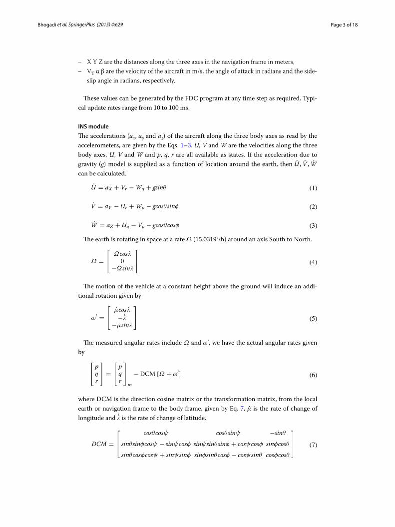
The accelerations (ax, ay and az) of the aircraft along the three body axes as read by the accelerometers, are given by the Eqs. 1–3. U, V and W are the velocities along the three body axes. U, V and W and p, q, r are all available as states. If the acceleration due to gravity (g) model is supplied as a function of location around the earth, then U , V , W can be calculated.
The earth is rotating in space at a rate Ω (15.0319°/h) around an axis South to North.
The motion of the vehicle at a constant height above the ground will induce an addi-tional rotation given by
The measured angular rates include Ω and ω′, we have the actual angular rates given by
where DCM is the direction cosine matrix or the transformation matrix, from the local earth or navigation frame to the body frame, given by Eq. 7, µ is the rate of change of longitude and is the rate of change of latitude.
(1)U = aX + Vr −Wq + gsinθ
(2)V = aY −Ur +Wp − gcosθsinφ
(3)W = aZ +Uq − Vp − gcosθcosφ
(4)Ω =
Ωcos0
−Ωsin
(5)ω′ =
µcos
−
−µsin
(6)
pqr
=
pqr
m
− DCM [Ω + ω′]
(7)DCM =
cosθcosψ cosθsinψ −sinθ
sinθsinφcosψ − sinψcosφ sinψsinθsinφ + cosψcosφ sinφcosθ
sinθcosφcosψ + sinψsinφ sinφsinθcosφ − cosψsinθ cosφcosθ

Page 4 of 18Bhogadi et al. SpringerPlus (2015) 4:629
U , V , W are integrated to calculate the velocity components (U, V, W), which are then transformed using the direction cosine matrix (Eq. 7) to give velocity along North (VN), velocity along East (VE) and downward velocity (VD) in the navigation frame or local earth frame.
VN, VE and VD are then integrated to give distances moved along the navigation axes (X, Y, Z) on the surface of the earth. If λ, µ and H denote the latitude, longitude and height of the aircraft at any instant, then the rate of change of latitude (Collison 1996; Etkin 1972) is given by
and rate of change of longitude is given by
where Re is the radius of the earth. The rate of change of altitude of the aircraft is given by
The position of the aircraft in terms of latitude, longitude and altitude can be thus cal-culated using Eqs. 9, 10 and 11.
From the time history, viz. p, q, r, ax,ay, az, the INS program now takes 6 states. These act as if the program is reading directly from the gyros and accelerometers. The four Euler parameters are calculated by the program. The Euler parameters are used to calculate the Euler angles. The U, V, W are computed from the accelerations of the accelerometers.
The velocity components of the aircraft are in the body frame. To convert it to the navigation frame or local earth frame, the DCM matrix is used and VT is calculated.
The positions X, Y, Z along the three axes in the local earth frame are obtained by inte-grating the velocity components. The latitude, longitude and height can be calculated. The fourth order Runge–Kutta method is used to carry out all the integrations. The INS module is shown in Fig. 2 (Vikas Kumar 2004).
GPS module
The latitude, longitude and altitude of the current location are given by the GPS receiver. The GPS program converts the X, Y, Z given out by the FDC into latitude, longitude and altitude as would be given out by the GPS receiver. The update rate is 1 s. WGS-84 approximation is used by the GPS program. The earth is considered as an ellipse with a semi-major axis (equatorial radius) of a = 6,378,137 m, and a semi-minor axis (polar radius) of b = 6,356,752.3142 m. The distance corresponding to a 1° change in longi-tude (Flon) and latitude (Flat) for a specified location (latitude and height or altitude) are defined.
(8)
X
Y
Z
=
VN
VE
VD
= DCMT
UVW
(9) = VN
Re
(10)µ = VE
Recos
(11)H = −VD

Page 5 of 18Bhogadi et al. SpringerPlus (2015) 4:629
Hence, the latitude and longitude from the previous location (λ1, μ1) are used to calcu-late the latitude and longitude at the current location (λ2, μ2).
where δX and δY are the changes in position along North and East directions on the Earth, respectively. The GPS module is shown in Fig. 3 (Vikas Kumar 2004).
(12)Flon = π
180
(
a2√a2cos2+ b2sin2
+ h
)
cos
(13)Flat =π
180
(
a2b2
(a2cos2+ b2sin2)32
+ h
)
(14)2 =δX
Flat+ 1
(15)µ2 =δY
Flon+ µ1.
Fig. 2 INS module
Fig. 3 GPS module

Page 6 of 18Bhogadi et al. SpringerPlus (2015) 4:629
Sensor modelling
Acceleration in terms of g is sent by the accelerometer to the INS in Volts. The scale fac-tor and the bias details are available from the specification sheets of the accelerometers. As the scale factor and the bias are not fixed, errors arise in the accelerations sensed by the accelerometers (Vikas Kumar 2004). They vary stochastically and are specified in the data sheets of the accelerometers.
The corresponding scale factors and offset biases are accounted in a similar way for the gyroscope error modelling (Vikas Kumar 2004). These errors together lead to drift, which grows with time in the output (location) given by the INS and it could be up to hundreds of meters. Table 1 gives a set of values given by the specification sheets which were used in the simulation (http://www.analog.com, ADXL212, Analog Devices Inc. 2013a, DXRS652, Analog Devices Inc. 2013b; http://www.falcom.com, GPS-Receiver JP3, Falcom Wireless Communications 2013). The temperature effects and the mis-alignment of accelerometers and gyroscopes also cause errors. These errors have been ignored.
Kalman filter module
The error dynamics model given in the works of Schmidt (1978), Bar-Itzhack et al. (1988), and Grewal et al. (2001) has been used for simulation. When the nominal equa-tions are perturbed in the local level north-pointing coordinate system that corre-sponds to the geographic location indicated by the INS, the error dynamics equations are obtained. The equations describing the propagation of the translatory and attitude errors describe the error behaviour of the INS. The translatory and the attitude errors are not coupled to each other. The nine state INS/GPS integration Kalman filter will then be built using the error dynamics equations. The perturbation of the position, velocity, attitude DCM, and gravity can be expressed as
(16)rn = rn + δrn
(17)vn = vn + δvn
(18)Cnb =
(
I − En)
Cnb
(19)γ n = gn + δ gn
Table 1 Sensor specifications used in simulation
Quality Value Standard deviation
Scale factor of the accelerometer 250 mV/g ±25/3 mV/g
0 g offset of the gyroscope 2500 mV ±625/3 mV
Scale factor of the gyroscope 1.11 mV/°/s ±10/3 %
Typical turn-on drift of the gyroscope 0.12°/s –
Random noise incorporated in the GPS – ±20 m

Page 7 of 18Bhogadi et al. SpringerPlus (2015) 4:629
where rn, vn and γn denote the position, velocity and gravity vectors respectively in the navigation frame, Cn
b denotes the attitude direction cosine matrix from the navigation frame to the body frame and En is the skew symmetric form of the attitude errors (ɛn)
and ^ and δ denote computed values and errors, respectively.The linear position error dynamics can be denoted by the perturbing Eqs. 9–11, which
are the dynamics equations for the geodetic positions. Since the position dynamics equations are functions of position and velocity, the position error dynamics equations are obtained using partial derivatives (Shin 2001).
where
and Re is the radius of the earth and is considered a constant. The velocity dynamics equation is expressed as
where f b is the acceleration of the aircraft in the body frame. The gravitation vector in the navigation frame gn, can be approximated by the normal gravity (0 0 γ )T, and γ varies with altitude. Assuming a spherical model, γ is given by
where γ0 is the normal gravity at h = 0. On perturbating Eq. 22 the velocity error dynam-ics equation can be obtained as (Shin 2001)
(20)En =
∈nX
=
0 −∈D ∈E
∈D 0 −∈N
−∈E −∈N 0
(21)δvδrn = Frrδrn + Fn
rv
Frr =
∂ ∂
∂ ∂µ
∂ ∂h
∂µ∂
∂µ∂µ
∂µ∂h
∂ h∂
∂ h∂µ
∂ h∂h
=
0 0−VN
(Re+h)2
VEsin
(Re+h)cos20
−VE
(RE+h)2cos
0 0 0
Frv =
∂ ∂VN
∂ ∂VE
∂ ∂VD
∂µ∂VN
∂µ∂VE
∂µ∂VD
∂ h∂VN
∂ h∂VE
∂ h∂VD
=
1
Re+h0 0
01
(Re+h)cos0
0 0 −1
(22)ˆvn = Cnb f
b −(
2Ω + ω′)× vn + γ n
(23)γ = γ0
(
Re
Re + h
)2
,
(24)δvn = Fvrδrn + Fvvδv
n +(
f nX)
∈n + Cnb δf
b

Page 8 of 18Bhogadi et al. SpringerPlus (2015) 4:629
where
and δfb is the perturbation in the acceleration vector in the body frame.The attitude error dynamics equation (Shin 2001) can be written as
where
and δωbib is the perturbation in the angular rate vector between the inertial frame and the
body frame.A state space model can be constructed by augmenting the Eqs. 21, 22 and 25 as
follows
where F is the dynamics matrix, X is the state vector, G is a design matrix, u is the forc-ing vector function (Shin 2001):
Fvr =
−2VEΩcos− V2E
(Re+h)cos20
−VNVD
(Re+h)2+ V
2Etan
(Re+h)2
2Ω(VNcos− VDsin)+ VEVN
(Re+h)cos20
VEVD
(Re+h)2− VNVEtan
(Re+h)2
2VEΩsin 0V
2E+V
2N
(Re+h)2− 2γ
(Re+h)
Fvv =
VD
Re+h−2Ωsin− 2
VEtan
Re+h
VN
Re+h
2Ωsin+ VEtan
Re+h
VD+VN tan
Re+h2Ωcos+ VE
Re+h
−2VN
Re+h−2Ωcos− 2
VE
Re+h0
(25)εn = Ferδrn + Fevδv
n +(
(Ω + ω′)X)
∈n − Cnb δω
bib
Fer =
−Ωsin 0−VE
(Re+h)2
0 0VN
(Re+h)2
−Ωcos− VE
(Re+h)cos20
VEtan
(Re+h)2
Fev =
01
Re+h0
−1
Re+h0 0
0−tan
Re+h0
(26)X = FX + Gu
F =
Frv Frv 0
Fvr Fvv (f bX)
Fer Fev −(
Ω + ω′X
x =
δrn
δvn
∈n
G =
0 0Cnb 00 −Cn
b
u =
δf b
δωbib

Page 9 of 18Bhogadi et al. SpringerPlus (2015) 4:629
The elements of u are white noise whose covariance matrix is given by
where the operator δ denotes the Dirac delta function whose unit is 1/time (Shin 2001). Q is called the spectral density matrix and has the form
where ϭa and ϭɷ are the standard deviations of the accelerometers and gyroscopes, respectively.
The Eq. 26 in discrete time form is given by
where Φk is the state transition matrix and wk is the driven response at tk+1 due to the presence of input white noise during time interval (tk, tk+1) (Brown and Hwang 1992). For the implementation of the INS, because the time interval Δt = tk+1 − tk is very small, the state transition matrix can be numerically approximate as
The covariance matrix associated with wk is
If the norm of Qk is larger than the real one, the Kalman filter trusts the measurements more than the system, thus making the estimates noisy due to free passage of measure-ment noise (Shin 2001). However, there is no time lag. If the norm of Qk is less than one, the time lag exists. When the norm of Qk is much smaller than the real one, the fil-ter diverges, which may result in numerical instabilities. Hence, for low inertial systems, Qk must be selected pessimistically so that the trajectory follows that of the GPS. The elements corresponding to δfz should be large enough so that they can account for the uncertainties in gravity as well as sensor imperfection.
The process noise, wk and the measurement noise, vk are uncorrelated, hence their covariance is 0. The covariance matrix for vk is given by
The Kalman filter is then implemented. The position from GPS is considered as meas-urements. The formulation of the measurement of the measurement equation can be written as
(27)E[u(t)u(t)T = Q(t)δ(t − T )
(28)Q = diag(
σ 2ax σ
2ay σ
2az σ
2ωx σ
2wx σ
2wz
)
(29)Xk+1 = ΦkXk + wk
(30)Φk = exp[Ft] ≈ I + Ft
(31)Qk = E[
wkwTk
]
≈ ΦKGQGTΦT
k t
(32)E[
vkvTk
]
= Rk
(33)zk = rnINS − rnGPS =
INS − GPS
µINS − µGPS
hINS − hGPS
Hk = I3x3|03x3|03x3

Page 10 of 18Bhogadi et al. SpringerPlus (2015) 4:629
Since λ and μ are in radians and hence very small, they cause numerical instabilities in calculating the Kalman gain Kk. Hence, the first two rows are multiplied by (Re +h) and (Re +h)cosλ, respectively (Shin 2001). The measurement equation now takes the form:
and the following measurement noise matrix has been used
which can be obtained from GPS processing. In our simulation, we have taken the error sphere of the GPS to have a radius of 20 m. Hence σ = σµ = σh = 20m.
The Kalman filter module is shown in Fig. 4 (Vikas Kumar 2004).The KF is a very effective stochastic estimator for a large number of problems, be it in
computer graphics or in navigation. It is an optimal combination, in terms of minimiza-tion of variance, between the prediction of parameters from a previous time instant and external observations at a present time instant.
zk =
(Re + h)(INS − GPS)
(Re + h)cos(µINS − µGPS)
hINS − hGPS
(34)Hk =
⟨
(Re + h) 0 0
0 (Re + h)cos 0
0 0 1
∣
∣
∣
∣
03x3
∣
∣
∣
∣
03x3
⟩
(35)Rk = diag(σ 2σ 2µ σ 2
h )
Fig. 4 Kalman filter module

Page 11 of 18Bhogadi et al. SpringerPlus (2015) 4:629
The MicroBlaze implementation of the GPS/INS integrated system on Virtex-6 FPGA is discussed in detail in the next section.
Implementation with MicroBlazeThis section describes the implementation of the above described algorithm. The micro-processors available for use in Xilinx FPGAs with Xilinx Embedded Development Kit (EDK) software tools can be broken down into two broad categories. There are soft-core microprocessors (MicroBlaze) and the hard-core embedded microprocessor (Power PC). The soft-core MicroBlaze microprocessor can be used in most of the Spartan-II, Spartan-3 and Virtex FPGA families. The hard-core embedded microprocessor is an IBM PowerPC 405 processor, which is only available in the Virtex-II Pro and Virtex-4 FX FPGA’s.
The MicroBlaze is a virtual microprocessor that is built by combining blocks of code called cores inside a Xilinx FPGA. The beauty to this approach is that as much micro-processor as needed can be developed. The project can be tailored to specific needs (i.e.: Flash, UART, General Purpose Input/output peripherals and etc.).
The MicroBlaze processor is a 32-bit Harvard Reduced Instruction Set Computer (RISC) architecture optimized for implementation in Xilinx FPGAs with separate 32-bit instruction and data buses running at full speed to execute programs and access data from both on-chip and external memory at the same time. The backbone of the archi-tecture is a single-issue, 3-stage pipeline with 32 general-purpose registers (does not have any address registers like the Motorola 68000 Processor), an arithmetic logic unit (ALU), a shift unit, and two levels of interrupt. This basic design can then be config-ured with more advanced features to tailor to the exact needs of the target embedded application such as: barrel shifter, divider, multiplier, single precision floating-point unit (FPU), instruction and data caches, exception handling, debug logic, fast simplex link (FSL) interfaces and others. This flexibility allows the user to balance the required per-formance of the target application against the logic area cost of the soft processor.
The MicroBlaze pipeline is a parallel pipeline, divided into three stages: fetch, decode, and execute. In general, each stage takes one clock cycle to complete. Consequently, it takes three clock cycles (ignoring delays or stalls) for the instruction to complete. Each stage is active on each clock cycle so three instructions can be executed simultaneously, one at each of the three pipeline stages. MicroBlaze implements an instruction prefetch buffer that reduces the impact of multi-cycle instruction memory latency. While the pipeline is stalled by a multi-cycle instruction in the execution stage the instruction prefetch buffer continues to load sequential instructions. Once the pipeline resumes exe-cution the fetch stage can load new instructions directly from the instruction prefetch buffer rather than having to wait for the instruction memory access to complete. The instruction prefetch buffer is part of the backbone of the MicroBlaze architecture and is not the same thing as the optional instruction cache.
The MicroBlaze core is organized as a Harvard architecture with separate bus interface units for data accesses and instruction accesses. MicroBlaze does not separate between data accesses to I/O and memory (i.e. it uses memory mapped I/O). The processor has up to three interfaces for memory accesses: local memory bus (LMB), IBM’s on-chip peripheral bus (OPB), and Xilinx cache link (XCL). The LMB provides single-cycle

Page 12 of 18Bhogadi et al. SpringerPlus (2015) 4:629
access to on-chip dual-port block RAM (BRAM). The OPB interface provides a con-nection to both on-chip and off-chip peripherals and memory. The cache link interface is intended for use with specialized external memory controllers. MicroBlaze also sup-ports up to 8 FSL ports, each with one master and one slave FSL interface. The FSL is a simple, yet powerful, point-to-point interface that connects user developed custom hardware accelerators (co-processors) to the MicroBlaze processor pipeline to accelerate time-critical algorithms.
All MicroBlaze instructions are 32 bits wide and are defined as either type A or type B. Type A instructions have up to two source register operands and one destination register operand. Type B instructions have one source register and a 16-bit immediate operand. Type B instructions have a single destination register operand. Instructions are provided in the following functional categories: arithmetic, logical, branch, load/store, and special. MicroBlaze is a load/store type of processor meaning that it can only load/store data from/to memory. It cannot do any operations on data in memory directly; instead the data in memory must be brought inside the MicroBlaze processor and placed into the general-purpose registers to do any operations. Both instruction and data inter-faces of MicroBlaze are 32 bit wide and use Big-Endian, bit-reversed format to represent data (order of bits: bit 0 bit 1 … bit 30 bit 31 with bit 0 the MSB and bit 31 the LSB). MicroBlaze supports word (32 bits), half-word (16 bits), and byte accesses to data mem-ory. Data accesses must be aligned (i.e. word accesses must be on word boundaries, half-word on half-word boundaries), unless the processor is configured to support unaligned exceptions. All instruction accesses must be word aligned.
The stack convention used in MicroBlaze starts from a higher memory location and grows downward to lower memory locations when items are pushed onto a stack with a function call. Items are popped off the stack the reverse order they were put on; item at the lowest memory location of the stack goes first and etc.
The MicroBlaze processor also has special purpose registers such as: program coun-ter (PC) can read it but cannot write to it, machine status register (MSR) to indicate the status of the processor such as indicating arithmetic carry, divide by zero error, a FSL error and enabling/disabling interrupts to name a few. An exception address register (EAR) that stores the full load/store address that caused the exception. An exception sta-tus register (ESR) that indicates what kind of exception occurred. A floating point status register (FSR) to indicate things such as invalid operation divide by zero error, overflow, underflow and denormalized operand error of a floating point operation.
MicroBlaze also supports reset, interrupt, user exception, break and hardware excep-tions. For interrupts, MicroBlaze supports only one external interrupt source (connect-ing to the interrupt input port). If multiple interrupts are needed, an interrupt controller must be used to handle multiple interrupt requests to MicroBlaze. An interrupt con-troller is available for use with the Xilinx EDK software tools. The processor will only react to interrupts if the interrupt enable (IE) bit in the MSR is set to 1. On an interrupt the instruction in the execution stage will complete, while the instruction in the decode stage is replaced by a branch to the interrupt vector (address 0 × 10). The interrupt return address (the PC associated with the instruction in the decode stage at the time of the interrupt) is automatically loaded into general-purpose register R14. In addition, the

Page 13 of 18Bhogadi et al. SpringerPlus (2015) 4:629
processor also disables future interrupts by clearing the IE bit in the MSR. The IE bit is automatically set again when executing the RTID instruction.
Writing software to control the MicroBlaze processor must be done in C/C++ lan-guage. Using C/C++ is the preferred method by most people and is the format that the Xilinx EDK software tools expect. The EDK tools have built in C/C++ compilers to gen-erate the necessary machine code for the MicroBlaze processor.
The MicroBlaze processor is useless by itself without some type of peripheral devices to connect to and EDK comes with a large number of commonly used peripherals.
The GPS/INS integration with Kalman filter implemented on Virtex-6 XC6VLX240T-1FFG1156 FPGA reconfigurable hardware is shown in Fig. 5 (http://www.xilinx.com, Virtex-6 FPGA and Xilinx 2013). The choice of reconfigurable hardware is based on the envisaged applications of this GPS/INS integration system in military and high speed avionics. The ML605 evaluation board from Xilinx is used as target hardware for hard-ware level verification.
The block diagram of the ML 605 evaluation board is shown in Fig. 6 (http://www.xilinx.com, Virtex6FPGA and Xilinx 2013).
The hardware software co-design flow with Xilinx’s MicroBlaze softprocessor core is adopted here. The INS data server, GPS data server are implemented as hardware intellec-tual property (IP) cores which provide the data samples to the MicroBlaze softprocessor. The INS and GPS data servers are the same as the INS and GPS modules that are already described in the previous sections. The Kalman filtering algorithm is implemented in C and ported to MicroBlaze along with its board support files. The IEEE 754 single precession floating point unit (FPU) core is added to MicroBlaze as a peripheral unit. The data taken for processing through Kalman filter is of floating point numbers with 6 fractional bits. The bit growth through Kalman filter processing is easily taken care for these fractional bits through single precision floating point numbers. Usage of double precision floating num-bers is always preferable but at the cost of increased resources in FPGA. The entire pro-cessor local bus (PLB) based hardware system configuration using Xilinx platform studio (XPS) is shown in Fig. 7 (http://www.xilinx.com, Virtex6FPGA and Xilinx 2013).
Fig. 5 ML605 evaluation board

Page 14 of 18Bhogadi et al. SpringerPlus (2015) 4:629
The USB-UART available on board is used for reading the algorithm inputs and outputs to personal computer (PC) for further analysis. The onboard JTAG debugger is used for configuration and runtime debugging. MATLAB is used for analyzing the logged data and results are presented in next section.
Fig. 6 Block diagram of ML605 evaluation board
Fig. 7 Hardware plat form with MicroBlaze and peripherals

Page 15 of 18Bhogadi et al. SpringerPlus (2015) 4:629
Results and discussionsThe data stored on the hard drive is input for the system. The program is run just as if the collection (of data) was taking place in real-time. Data is taken from FDC for 10 ms and analysis is done through MATLAB. The trajectories obtained from the FDC in MATLAB give the simulated sensor data. The stored Aircraft states were used to sim-ulate sensors. The prediction accuracy of INS is analyzed by comparing it with a true trajectory generated using MATLAB. Various errors in inertial sensors and the GPS are included in the simulation results. Same sensor outputs were given to the present MicroBlaze implementation on Vitex-6 FPGA and the results were compared. The out-put waveforms obtained from the GPS/INS integrated system, the GPS, and the actual trajectory are shown in Figs. 8, 9 and 10. The plots for latitude, longitude, and altitude obtained directly from the hardware (Virtex-6 FPGA output) are shown in Figs. 11, 12 and 13. They show good agreement with the actual trajectory.
Fig. 8 Distance along North as given by the Kalman filter
Fig. 9 Distance along East as given by the Kalman filter

Page 16 of 18Bhogadi et al. SpringerPlus (2015) 4:629
Fig. 10 Altitude as given by the Kalman filter
Fig. 11 Virtex-6 FPGA (hardware) output. Latitude versus time
Fig. 12 Virtex-6 FPGA (hardware) output. Longitude versus time

Page 17 of 18Bhogadi et al. SpringerPlus (2015) 4:629
The resource utilization report of the developed system on Virtex-6 FPGA is given in Table 2. As the area consuming algorithm blocks are implemented on MicroBlaze and performance demanding blocks are implemented on FPGA fabrics, the implemented system demonstrates optimal area occupancy and high speed implementation.
The maximum clock speed achieved by MicroBlaze softprocessor is 130 MHz. The present system is tested at 88 MHz clock speed. The FPGA running for the total inte-grated system is profiled for speed and latencies by running it for 900 s of data.
The Kalman filter iterations are presently being computed at 10 ms interval. However the implemented logic is able to achieve the latency of 0.9 ms for every iteration. Hence the present system can integrate with INS system with an update rate of 1 ms.
Concluding remarksThe paper discussed a better approach to fuse the data from the GPS and INS using Kalman filter. The position accuracy of the GPS/INS system is comparable to that of the GPS receiver over a span of 250 s.
The implemented system with hardware software co-design approach occupies only 5 % of slices and 1 % of DSP48 resources, with maximum achievable clock speed of 130 MHz. The latency for one iteration of Kalman filter is less than 1 ms, hence suitable for integrating with high speed INS units. The Virtex-6 FPGA consumes 4285 mW of power. The Kalman filter implemented on Virtex-6 FPGA shows promising results by
Fig. 13 Virtex-6 FPGA (hardware) output. Altitude versus time
Table 2 Resource utilization of Virtex-6 FPGA
Resource Total available Used Utilization (%)
Slice registers 3,01,440 7101 2
Slice LUTs 1,50,720 7925 5
BRAM 416 70 16
DSP48 768 5 1

Page 18 of 18Bhogadi et al. SpringerPlus (2015) 4:629
using reconfigurable hardware software co design approach for future GPS/INS inte-grated navigation systems. The power consumption is calculated for the operating clock rate of 100 MHz.Authors’ ContributionsLRB, SRG and VVSRK were involved in the conception and design, acquisition of data, analysis and interpretation of data; drafting the manuscript or revising it critically for important intellectual content; final approval of the version to be published; and agree to be accountable for all aspects of the work in ensuring that questions related to the accuracy or integrity of any part of the work are appropriately investigated and resolved. All authors read and approved the final manuscript.
Competing interestsThe authors declare that they have no competing interests.
Received: 19 January 2015 Accepted: 22 September 2015
ReferencesAgarwal V, Arya H, Bhaktavatsala S (2009) Design and development of a real-time DSP and FPGA-based integrated GPS-
INS system for compact and low power applications. IEEE Trans Aerosp Electron Syst 45(2):443–454ADXL212, Analog Devices Inc. (2013a) http://www.analog.com/en/products/mems/mems-accelerometers/adxl212.html.
Accessed 12 Dec 2013DXRS652, Analog Devices Inc. (2013b) http://www.analog.com/en/products/mems/mems-gyroscopes/adxrs652.html.
Accessed 12 Dec 2013Bar-Itzhack IY, Berman N (1988) Control theoretic approach to inertial navigation systems. J Guid 11(3):237–245Brown RG, Hwang PYC (1992) Introduction to random signals and applied Kalman filtering. Wiley, New YorkCao FX, Yang DK, Xu AG, Ma J, Xiao WD, Law CL, Ling KV, Chua HC (2002) Low cost SINS/GPS integration for land vehicle
navigation. In: IEEE 5th international conference on intelligent transportation systems, pp 910–913Collison RPG (1996) Introduction to avionics. Chapman and Hall, LondonEtkin B (1972) Dynamics of atmospheric flight. Wiley, TorontoFaulkner NM, Cooper SJ, Jeary PA (2002) Integrated MEMS/GPS navigation systems. In: IEEE position location and naviga-
tion symposium, pp 306–313GPS-Receiver JP3, Falcom Wireless Communications (2013) http://www.falcom.de/falcom/news/news-view/gps-receiver-
falcom-kp3-available.pdf and http://www.casde.iitb.ac.in/MSL/motion/gps/jp3manual.pdf. Accessed 12 Dec 2013Grewal MS, Weill LR, Andrews AP (2001) Global positioning systems. Inertial navigation, and integration. Wiley, New YorkHegg J (2002) Enhanced space integrated GPS/INS (SIGI). In: IEEE aerospace and electronic systems magazine, pp 26–33Jaffe R, Qi H, Carter P, Madni AM, MMQ-G (2005) A low cost MEMS INS-GPS. In: ION GNSS 18th international technical
meeting of the satellite division, Long Beach, CA, pp 956–966Moon SW, Hwang DH, Sung TK, Lee SJ (1998) Design and implementation of an efficient loosely-coupled GPS/INS inte-
gration scheme. Technical Report, Chungnam National University, KoreaSchmidt GT (1978) Strapdown inertial systems—theory and applications. AGARD Lecture Series, No. 95Shin EH (2001) Accuracy improvement of low cost INS/GPS for land application. M.Sc. Thesis. University of Calgary,
Geomatic Engineering DeptVikas Kumar N (2004) Integration of inertial navigation system and global positioning system using Kalman filtering.
M.Tech Dissertation, Indian Institute of Technology, India, pp 20–30Virtex-6 FPGA, Xilinx (2013) http://www.xilinx.com/support/documentation/data_sheets/ds150.pdf. Accessed 12 Dec
2013