Embed Size (px)
DESCRIPTION
Theory of LBM
Citation preview

The Lattice Boltzmann Equation Method:Theoretical Interpretation, Numerics and
Implications
R.R. Nourgaliev, T.N. Dinh, T.G. Theofanous, and D. Joseph �
Center for Risk Studies and Safety, University of California, Santa Barbara, USA�Aerospace Engineering and Mechanics, University of Minnesota, USA
E-mail: [email protected]; [email protected]; [email protected]; [email protected]
During the last ten years the Lattice Boltzmann Equation (LBE) method has been
developed as an alternative numerical approach in computational fluid dynamics
(CFD). Originated from the discrete kinetic theory, the LBE method has emerged
with the promise to become a superior modeling platform, both computationally
and conceptually, compared to the existing arsenal of the continuum-based CFD
methods. The LBE method has been applied for simulation of various kinds of fluid
flows under different conditions. The number of papers on the LBE method and its
applications continues to grow rapidly, especially in the direction of complex and
multiphase media.
The purpose of the present paper is to provide a comprehensive, self-contained and
consistent tutorial on the LBE method, aiming to clarify misunderstandings and
eliminate some confusion that seems to persist in the LBE-related CFD literature.
The focus is placed on the fundamental principles of the LBE approach. An excur-
sion into the history, physical background and details of the theory and numerical
implementation is made. Special attention is paid to advantages and limitations of
the method, and its perspectives to be a useful framework for description of complex
flows and interfacial (and multiphase) phenomena. The computational performance
of the LBE method is examined, comparing it to other CFD methods, which directly
solve for the transport equations of the macroscopic variables.
1
2 NOURGALIEV, DINH, THEOFANOUS, AND JOSEPH
CONTENTS1. Introduction .2. Origin and basic idea of the lattice Boltzmann equation method .3. Numerical implementation of the LBE method .4. Lattice Boltzmann models for hydrodynamics of complex fluids .5. Derivation and analysis of the continuum equivalent of the LB equation .6. Computational efficiency .7. Concluding remarks .
A. Lattice geometry and symmetry.
B. Equilibrium distribution function.C. Multiphase flow modeling.D. Derivation of the viscous stress tensor for the LBGK models.
E. Evaluation of the deviations from the Navier-Stokes equations.
1. INTRODUCTION
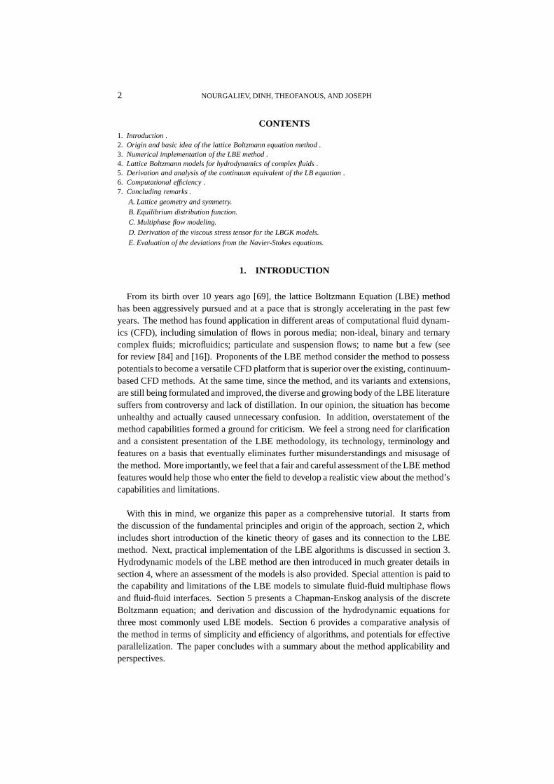
From its birth over 10 years ago [69], the lattice Boltzmann Equation (LBE) methodhas been aggressively pursued and at a pace that is strongly accelerating in the past fewyears. The method has found application in different areas of computational fluid dynam-ics (CFD), including simulation of flows in porous media; non-ideal, binary and ternarycomplex fluids; microfluidics; particulate and suspension flows; to name but a few (seefor review [84] and [16]). Proponents of the LBE method consider the method to possesspotentials to become a versatile CFD platform that is superior over the existing, continuum-based CFD methods. At the same time, since the method, and its variants and extensions,are still being formulated and improved, the diverse and growing body of the LBE literaturesuffers from controversy and lack of distillation. In our opinion, the situation has becomeunhealthy and actually caused unnecessary confusion. In addition, overstatement of themethod capabilities formed a ground for criticism. We feel a strong need for clarificationand a consistent presentation of the LBE methodology, its technology, terminology andfeatures on a basis that eventually eliminates further misunderstandings and misusage ofthe method. More importantly, we feel that a fair and careful assessment of the LBE methodfeatures would help those who enter the field to develop a realistic view about the method’scapabilities and limitations.
With this in mind, we organize this paper as a comprehensive tutorial. It starts fromthe discussion of the fundamental principles and origin of the approach, section 2, whichincludes short introduction of the kinetic theory of gases and its connection to the LBEmethod. Next, practical implementation of the LBE algorithms is discussed in section 3.Hydrodynamic models of the LBE method are then introduced in much greater details insection 4, where an assessment of the models is also provided. Special attention is paid tothe capability and limitations of the LBE models to simulate fluid-fluid multiphase flowsand fluid-fluid interfaces. Section 5 presents a Chapman-Enskog analysis of the discreteBoltzmann equation; and derivation and discussion of the hydrodynamic equations forthree most commonly used LBE models. Section 6 provides a comparative analysis ofthe method in terms of simplicity and efficiency of algorithms, and potentials for effectiveparallelization. The paper concludes with a summary about the method applicability andperspectives.

THE LBE: THEORETICAL INTERPRETATION, NUMERICS AND IMPLICATIONS 3
2. ORIGIN AND BASIC IDEA OF THE LATTICE BOLTZMANN EQUATIONMETHOD
2.1. Boltzmann equation and kinetic theory of gases
The purpose of this section is to outline the most important facts and results of the ki-netic theory which are relevant to the lattice Boltzmann equation method. More exhaustiveoverview of the kinetic theory and recent important developments can be found in [15];[49]; [55]; [64]; [14]; [39]; [57] and [21].
Kinetic theory. The Lattice Boltzmann Equation method originates from the kinetictheory of gases. The primary variable of interest is a one-particle probability distributionfunction (PPDF), ���� �� ��, so defined that
����� �� �� � ��� � ���
�is the number of particles
which, at time �, are located within a phase-space control element���� � ���
�about � and
� (� is a particle’s coordinate in physical space and � is a particle’s velocity). The transportequation for the PPDF can be expressed as [49]:
���� � � �
�� � � �
�� ���� �� �� � ��
���
coll(1)
where � is the external force acting on the particle.
Boltzmann equation.To derive the Boltzmann equation from equation (1), the collisionterm �����coll has to be explicitly specified. Two major assumptions were made [49]: (a)only binary collisions are taken into account. This is valid if the gas is sufficiently dilute(ideal gas). (b) The velocity of a molecule is uncorrelated with its position 1 . The lastassumption is known as the assumption of molecular chaos. Importantly, without thisassumption, the collision operator �����coll would not be expressible in terms of � itself.Instead, it would involve a two-particle probability distribution function. In general case,equation (1) can be replaced by a set of � coupled equations to account for multi-particleinteractions (BBGKY equations).
Under the assumptions made, Boltzmann [12] expressed the collision term of equation(1) as2 [15] [49] [55]:
�����coll �
���
����������
����� ������� �� �� ���� � �� ���
�(2)
where � is the scattering angle of the binary collision���� �����
� � ��� ����
�with fixed
�; � and � � denote the PPDF before and after collision; and ��� is the differential crosssection of this collision, [49].
�In fact, two other assumptions were also made: (c) wall effects are ignored and (d) the effect of the externalforce on the collision cross section is neglected.
�Boltzmann’s derivation of the collision integral, eq.(2), was, even though intuitive, deeply insightful. There isa gap between Newton’s equations of motion of the molecules constituting a gas and the Boltzmann equation (2).Nevertheless, this equation is known to be valid, and it has been successfully applied to study transport propertiesof dilute gases [55]. A more general BBGKY theory (due to Bogoliubov, 1946 [11], Kirkwood, 1947 [54], andGrad, 1949 [35]) was developed to provide a consistent derivation of the Boltzmann equation.

4 NOURGALIEV, DINH, THEOFANOUS, AND JOSEPH
Boltzmann’s ‘� theorem’. Introducing the functional � as the complete integral definedby the equation
� �
�� �� � �� (3)
the Boltzmann ‘� theorem’ states that if the PPDF, � , satisfies the Boltzmann transportequation (1) and (2), then � is a non-increasing in time function, �����
�� � �. This is theanalog of the second law of thermodynamics, if we identify � with the negative of theentropy per unit volume divided by Boltzmann’s constant, � � � �
� ��. Thus, the ‘�
theorem’ states that, for a fixed volume , the entropy never decreases, [12] and [49].
Collision interval theory. The collision integral, eq.(2), can be significantly simplifiedfor near-equilibrium states. The collision interval theory states that during time interval Æ �a fraction Æ��� � �
�� of the particles in a given small volume undergoes collisions, whichalter the PPDF from � to the equilibrium value given by the Maxwellian:
� eq �
���� �����
��
� ��� ���
��
(4)
where��,�,� , and� are the dimension of space,gas constant, temperature, macroscopicdensity and velocity, respectively. Thus, the collision term can be expressed in the formknown as the ‘BGK collision operator’, [7] and [15]:
�����coll � �� � � eq
�� �� � � eq
���(5)
where � is a relaxation time3�4. The Boltzmann equation with the BGK collision operatorhas the following form:
��� � � � ��� � � � ��� � �� � � eq
�(6)
Simplification of the forcing term. In order to evaluate the forcing term, the derivative��� has to be explicitly given. The following assumption is made [44]:
��� � ���eq (7)
which is due to the fact that � eq is the leading part of the distribution function � (‘anassumption of small deviation from the equilibrium’). By combining the Maxwellianeq.(4) with eq.(7) and eq.(6), the following equation is obtained:
��� � � � ��� � �� � � eq
��
� � ��� ��
��� eq (8)
�The BGK equation (5) is a phenomenological equation [64]. This characteristic pre-determines the domainof the equation’s applicability: dilute gases in a state close to thermal equilibrium. The inaccuracy of the BGKequation is enhanced when one treats the equation by the Chapman-Enskog method [55].
�The ‘� theorem’ remains valid for the BGK equation, [55].

THE LBE: THEORETICAL INTERPRETATION, NUMERICS AND IMPLICATIONS 5
Link to hydrodynamics. Connection of the Boltzmann equation to the hydrodynamicsis accomplished through the integration in the particle momentum space:
�� � � ��� � �
� � � �� ��� � � �
�
� �� � ��� ��
� ��
�� � eq� ��� � �
� � eq � �� ��� � � �
�
� �� eq � ��� ��
� ��
(9)
with the kinetic energy � given by
� � ��
� ��� � ��
���
(10)
where �� and �� are the Avogadro’s (or Loschmidt’s [15]) number and the Boltzmannconstant, respectively. �� is the number of degrees of freedom of a particle (� � � � and �
for monoatomic and diatomic gases, respectively).
2.2. Lattice Boltzmann equation
2.2.1. Heuristic approach
Historically, the ‘classical’ LB equation has been developed empirically, with basic ideaborrowed from the cellular automata fluids, [31] and [103]. The physical space of interestis filled with regular lattice populated by discrete particles. Particles ‘jump’ from one siteof the lattice to another with discrete particle velocities ��, (� � �� ���� �, where � is thetotal number of possible molecule’s directions), and colliding with each other at the latticenodes, Figs.1a,1b. The lattice geometry (a set of possible particle velocities) should obeycertain symmetry requirements (see Appendix A), which are compelling in order to recoverthe rotational invariance of the momentum flux tensor at the macroscopic level [103].
X
Diagonal sublattice (q=2), (+/-1,+/-1)
Orthogonal sublattice (q=1), cyc:(+/-1,0)
Y
The cell itself (q=0), (0,0,0)
1
34
5
7 8
0
2
6
The cell itself (q=0), (0,0,0)
Z
X
Y
Primitive cubic sublattice (q=1), cyc:(+/-1,0,0)
Body-centered cubic sublattice (q=2), (+/-1,+/-1,+/-1)
26
0
1
2
3
4
5
6
78
9 10
1112
13 14
15
16
17
18
19
20
21
22
23
24
25
a) b)
FIG. 1a. Lattice geometry and velocity vectors of the two-dimensional nine-speed ���� model.
FIG. 1b. Lattice geometry and velocity vectors of the three-dimensional fifteen-speed ����� model.

6 NOURGALIEV, DINH, THEOFANOUS, AND JOSEPH
In effect, the LBE method corresponds to the following formal discretization in the phasespace of the Boltzmann equation:
a) � � ��b) � � ��
c) � �� � ���� � �� ������� � ���
� ���������� ��
(11)
where the discrete equilibrium distribution function, also called “the Chapman-Enskogexpansion”, is inspired by the following constant-temperature and small velocity (low-Mach-number) approximation of the Maxwellian eq.(4)
��� � � ��
�� ��
�
���� �����
�� �
�� � ����
��� � ������ ��
� ��
��
������ (12)
Thus, the lattice Boltzmann BGK equation is heuristically postulated as5
���� � �������� �� �Advection operator,�����
� ��� � � eq�
���� � ���� � ���
��� eq�� �� �
Collision operator, ����
(13)
As a next step, one can define the “LBE sound speed” as [43]
���
��� (14)
Remark 1:
At this point, a principal departure from the actual kinetic theory must be emphasized.
According to the kinetic theory [15], the speed of sound is related to the temperature as
�� �� (15)
where � ����
� � ��� is a ratio of specific heats. The definition eq.(14) means that the
LBE’s pseudo-molecules must have infinite number of degrees of freedom,�� �, which, ofcourse, does not make any physical sense. As we show further below (section 3.3), if the fluid being modeled is to retain its speed
of sound, the solution of eq.(13) is impossible for all practical purposes. As a consequence,compressibility effects are outside the realm of the LBE method; �� is retained, however, witha totally different meaning and role - that of a pseudo-compressibility parameter that allows thesolution to relax to the appropriate incompressible viscous solution.
Rather than “sound speed”, let us call, therefore, �� by the name “Pseudo-Sound-Speed” (“PSS”).Furthermore, as a consequence, the relaxation time and related molecular mean free path and ve-locity also change their meaning and they would be called as “Lattice relaxation time”, “Latticemean free path” and “Lattice velocity”, respectively. While this departs from the normal us-age, adoption of these terms, we believe, will clear up an enormous conceptual barrier for thenewcomers and uninitiated.
�We have limited our study to the BGK LBE models, which are currently in the mainstream of the LBEtechnology. There are several non-BGK LBE models available in the literature. McNamara et al. pursue anapproach with multi-particle collision operator [70]; [71] and [72]. Similar approach is utilized by Eggels andSomers ([25] and [26]). Another recent development of the non-BGK LBE is due to Lallemand and Luo, [60].While being more sophisticated both conceptually and technically, these models are believed to be more stableand more flexible in implementation of variable fluid properties.

THE LBE: THEORETICAL INTERPRETATION, NUMERICS AND IMPLICATIONS 7
The coefficients��� ��� �� and�� of the ‘Chapman-Enskog’ expansion for � eq� , eq.(11),
are ‘tuned’ to recover mass, momentum conservation and viscous stress tensor during themultiscale Chapman-Enskog perturbative expansion procedure 6.
Eqs.(13) are the coupled system of Hamilton-Jacobi equations,with Hamiltonian � ������,and the ‘coupling’ source term given by the collision operator. This system can be solvedby any appropriate numerical scheme (see section 3).
2.2.2. Consistent discretization
Recent studies by He and Luo [42] [43] pioneer another way to establish the LBEmethodology. In particular, He and Luo [43] demonstrated that the lattice Boltzmann equa-tion can be viewed as a special finite-difference approximation of the Boltzmann equation.The chief idea and motivation are to provide a sound theoretical foundation for a transitionfrom the ‘continuous’ Boltzmann equation to the LBE, which involves the choice of thediscrete particle velocities (structure of the lattice) and the choice of the coefficients ofexpansion for equilibrium distribution function, eq.(11). There are two major ingredientsin the procedure by He and Luo, discussed below.
Time discretization. Eq.(6) is integrated over a time step �:
� ��� � � �� �� �� ��� � ��� �� �� � � � ����
���eq
� ���
�� ����
������� � eq
(16)
The first integral in the collision operator is treated explicitly, using the first-order ap-proximation, while the second one can be treated using the trapezoidal implicit scheme[44], which, in order to regain the explicitness of the method, entails the following variabletransformation:
� � � � � � ��� ��
��� eq� (17)
Thus, the first-order time discretization yields the following Boltzmann equation:
� ��� � � �� �� �� ��� � ��� �� �� � �����������eq��������
where �eq ���� �������
�����
� eq (18)
Note, that the speed of sound is defined by eq.(14).
Phase space discretization.This step establishes the structure of the lattice and theform of the equilibrium distribution function. To derive a “consistent” LBE scheme, theintegration in momentum space eq.(9) has to be approximated by the following quadrature[43]: �
����� eq��� �� ���� ���
��������eq� ��� ��� �� (19)
�In the case of the ‘thermal’ LBE, it is also required to conserve energy, which would entail addition of theexpansion terms in the Taylor series eqs.(11) and (12).

8 NOURGALIEV, DINH, THEOFANOUS, AND JOSEPH
where���� � �� � � �� ���� �� ������ ���� and�� are the polynomials of � and the ‘weight’coefficient of the quadrature, respectively. Eq.(19) corresponds to the following ‘link’ ofthe LBE to hydrodynamics7:
��
� ��� � ��
� �� � ��� � � ��
�� �� � ��� � ��
�
��
� �eq� � � �
�� �
eq� � ��� � � �
�
�� �
eq� � ��� � ��
� (21)
where
����� �� � �� ���� ��� ��� � eq� ��� �� � �� �
eq��� ��� �� (22)
Now, a task is to properly specify the abscissas of the quadrature eq.(19), or, in otherwords, the ‘structure’ (‘symmetry’) of the lattice. To do that, one must impose a set ofconstraints for this ‘structure’. These constraints are formulated based on the Chapman-Enskog procedure to ‘link’ the Boltzmann equation to the Navier-Stokes equations, seesection 5.1, which involves the following moments of the equilibrium distribution function:
Mass conservation: ���� � �� � � and � ��Momentum conservation: ���� � �� � � � �� � and � ����Energy conservation: ���� � �� � � � �� � � ����� and � ������
(23)
Thus, the basic idea is that with the chosen abscissas of the quadrature eq.(19), the momentsof � eq
� , eq.(23), should be calculated exactly. With this, the Chapman-Enskog procedureis intact, and it is argued that the framework of the lattice Boltzmann equation can rest onthat of the Boltzmann equation, and the rigorous results of the Boltzmann equation can beextended to the LBE via this explicit connection [42].
Remark 2:
It is instructive to note that the Maxwell-Boltzmann equilibrium distribution function �eq is anexact solution of the Chapman-Enskog zero-order approximation of the Boltzmann equation [49].In finding the abscissas of the quadrature eq.(19), however, instead of the exact Maxwellian, itsconstant-temperature and low-Mach-number approximation eq.(12) is utilized, [43], with whichno rigorous link to the Navier-Stokes equations is available. Moreover, this is exactly the reasonwhy the Boltzmann’s “� theorem” does not hold for the LBE. Therefore, this procedure does notprovide a substitute for the Chapman-Enskog multiscale perturbative expansion procedure (seesection 5.1)
The details of the procedure to find the required abscissas of the quadrature and corre-sponding approximations of the Maxwellian are given in [43] for two-dimensional 6-, 7-and 9-bit and three-dimensional 27-bit lattice models. It is important to note that with thisprocedure, the ‘weighting’ coefficients for the ‘composing’ sublattices and the coefficientsof the equilibrium distribution function are exactly the same as those of the ‘heuristic’ LBE,
�In the case of the transformation eq.(17), � is substituted by �, and the first momentum is modified as
��� ����� �
��� � �� ��� ��� �
���� �
���eq � �� �� (20)

THE LBE: THEORETICAL INTERPRETATION, NUMERICS AND IMPLICATIONS 9
summarized in Appendices A and B, providing that 8 ��� � ��
��� , [45].
2.2.3. Non-dimensional form
To cast the discrete Boltzmann equation (13) into the non-dimensional form, one mustintroduce the following characteristic scales9:
Characteristic length scale: �
Characteristic velocity: ��
Reference density:
Lattice mean free path: �
(24)
Using these scales, the variables utilized in the LBE theory are non-dimensionalized as
Non-dimensional variables:PPDF: ��� � ��
��
Lattice velocity: ���� ������
Time: �� � ���
�
Length: �� � ��
Density: � � ��
Macroscopic velocity: �� � ����
Pseudo-sound-speed: ��� � ����
Body force: ��� ����
��
�
� ���
Kinematic viscosity: �� � ����
� ���
(25)
where � is a unit-vector, specifying the direction of the body forces.
To make a non-dimensional relaxation time, we will use the lattice Knudsen numberdefined as a ratio of the lattice mean free path � to the flow characteristic length scale �:
� ��
�(26)
Defining the “collision time” as �� � ���
, the dimensionless relaxation time is
�� ��
���
���
��
��
�(27)
where the scaling “lattice-molecular velocity” is defined as � � �� .
In the ‘heuristic’ LBE models, the lattice symmetry parameters ��� and ��� are adjustable, with free
parameter ��, allowing to vary the pseudo-sound-speed. For ����, the requirement ��� � �
�� is satisfied with
�� � ��
.�As explained in Remark 1, we add the ‘prefix’ “lattice”, emphasizing the artificial nature of the LBE’s
“pseudo-molecules”; and, correspondingly, of the LBE’s mean free path, sound speed, etc.
10 NOURGALIEV, DINH, THEOFANOUS, AND JOSEPH
With this dimensionalization introduced, the discrete Boltzmann equation (13) is trans-formed into the following non-dimensional equation:
������ � �������
��� � ���� � �� eq
�
����
��� � ����� � ����
����
�� eq� (28)
For the most of the paper, for compactness, the hat ���� is omitted; and, unless explicitlyspecified, all variables are assumed to be non-dimensional.
3. NUMERICAL IMPLEMENTATION OF THE LBE METHOD
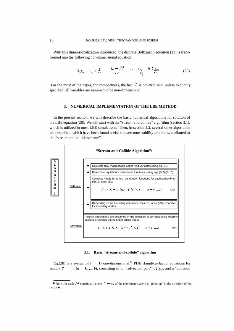
In the present section, we will describe the basic numerical algorithms for solution ofthe LBE equation (28). We will start with the “stream-and-collide” algorithm (section 3.1),which is utilized in most LBE simulations. Then, in section 3.2, several other algorithmsare described, which have been found useful to overcome stability problems, attributed tothe “stream-and-collide scheme”.
ALGORITHM
I
“Stream-and-Collide Algorithm”:
Collision:
Calculate flow macroscopic conserved variables using eq.(21).
Determine equilibrium distribution functions, using eqs.(B.2)-(B.10).
Compute ’ready-to-advect’ distribution functions for each lattice direc-tion, at each site:
��� ��� �� ����� �� � ���� ��� � �� ���� � (29)
Depending on the boundary conditions, the r.h.s. of eq.(29) is modifiedfor boundary nodes.
Advection:
Particle populations are streamed in the direction of corresponding discretevelocities, towards the neighbor lattice nodes.
�� �� � ���� �� �� ��� ��� ��� � �� ���� � (30)
3.1. Basic “stream-and-collide” algorithm
Eq.(28) is a system of �� � �� one-dimensional10 PDE Hamilton-Jacobi equations forscalars � ��, (� � �� ���� �), consisting of an “advection part”, � � �, and a “collision
��Note, for each ��-equation, the axis � �� of the coordinate system is “pointing” in the direction of thevector �� .

THE LBE: THEORETICAL INTERPRETATION, NUMERICS AND IMPLICATIONS 11
part”, � � �:
�
���
Æ
�
�
�!� �� �����
��� �
�(31)
where �� �� is a step of space discretization in !�� "��-direction; and the collisionoperator is � � � � � ����� �
�� .
The simplest scheme for discretization of each of these equations involves a first-order-accurate implicit forward differencing for the advection part,
� � � �
����� �
���
��
Æ
�
����� �� �
�����
Æ
and a first-order-accurate explicit Euler discretization for the collision part, � ���� [94]. This
results in the “basic” two-step “stream-and-collide” LBE algorithm 11 (see Algorithm I).
3.2. Advanced Numerical Schemes
3.2.1. Numerical discretization of the advection operator
Let’s consider general three-point finite-difference formula for discretization of eq.(31),at point # in “���” direction of the particle’s motion12:
��� � �
�� � �
� �
�� �� (32)
The upper indices denote the level of implicity: � � $ (explicit), � � $ � �� (semi-implicit), and � � $�� (implicit). Eq.(32) can be written in the following “conservative”form, [76]:
��� � � � �
�
�CFL � �
�� �� � �� CFL � �
�� � ���
�
���
�����
� ��
� �� � �� ������
� ��
� � ��� � �
(33)
where ������
��
are the dimensionless coefficients of numerical diffusion, and
� � ������
� ��
� �� CFL � �
�
� � �� �� CFL � �
�� �
� CFL � ��� �
�����
� ��
� ������
� ��
� � ������
� ��
� �� CFL � �
�
(34)
Application of eqs.(32)-(34) to the ’stream-and-collide’ equations (29-30) gives � ����� �
��, [94]. This numerical diffusion can be compensated for by modifying the relaxation
��It is instructive to note that with chosen notation �� ��� ���� � �� � �������� .
��It is instructive to note that, in the present section, “�” is a point of the finite-difference discretization ofeq.(31), discretized in the ��-direction.

12 NOURGALIEV, DINH, THEOFANOUS, AND JOSEPH
parameter from � � to (�� � ��).
For the “stream-and-collide” scheme, the “Courant, Friedrichs, and Lewy” number foradvection is CFL � ��Æ�
���� �. This condition CFL=1 is quite restrictive, especially in
the case of the strong non-linearity of the collision operator 13. The following ‘predictor-corrector’ algorithm has been introduced in [74], allowing to overcome this problem.
ALGORITHM
II
“Multifractional stepping procedure (MF �)”:
In this scheme, a time step from � to �� � is divided in to �� sub-steps.
The downwind/upwind difference are employed for an advection term, at eachodd/even sub-step:
������ �
��� �
����
�������
�� ������
������ �
����� �
�������� ������
��� �
�����
� �� ���� ��� ��
(35)
With this scheme, the CFL number can be varied arbitrarily, CFL= ��� . For � � �, this
scheme is identical to the explicit MacCormack scheme [76]. Furthermore, for each coupleof sub-steps, the central differencing is applied in both time and space, rendering thus thesecond-order accuracy. Applying eqs.(32)-(34), the sub-step coefficient of the numericaldiffusion is ������� � � �
�� for odd sub-steps, and � ������ � � ��� for even sub-steps. Thus,
the resulting coefficient of the numerical diffusion is zero.
Other algorithms for discretization of the LBE’s advection operator were also proposedto help alleviating a stability problem in the LBE numerical treatment; see [98] (“TVD/AC”scheme) and [71] (“Lax-Wendroff” scheme). The stability problem is even more acute inthe simulation of multiphase and thermal flows ([74], [98], [71]).
3.2.2. Numerical discretization of the collision operator
The ‘stream-and-collide’ LBE numerical scheme employs the explicit Euler method forthe collision operator. In the case of% � �
�� � , and in the case of the strong non-linearityof the collision operator, this scheme fails to produce stable solutions [94] [74]. Notice,that the LBE equations (31)
�����
%� � �� � �� �� � � ���
� � ���
(36)
��For example, in the case of the complex fluids, section 4.

THE LBE: THEORETICAL INTERPRETATION, NUMERICS AND IMPLICATIONS 13
are stiff differential equations in %: �� � �� . This means, that an error would growexponentially.
Several numerical schemes were developed for the solution of stiff differential equations(see for review [76]). For example, the first- and the second-order explicit Runge-Kuttamethods can be used to reduce the error growth, [74]. It is instructive to note that theRunge-Kutta schemes do not guarantee stability for the stiff equations. To address thisproblem, Nourgaliev et al. developed an implicit trapezoidal method (IT) [74] (AlgorithmIII).
ALGORITHM
III
“Implicit Trapezoidal method (IT)”:
Collision:
����� �� �Euler�;�Beginning of the iteration loop, � �� �:
“Predict” collision term: �� �������� .
Relaxation (optional):�� ! � �� � ��� !� � ���� ; ! - is a relaxation parameter.
Advection: ����� � �
�
�. Obtain new ��
� .
Calculate new macroscopic variables: ���� �� "�� �� �
��� ��
�.
("�� - is a pressure tensor, section 5).
Calculate new equilibrium distribution function �� �� from
���� �� "�� �� .
Determine new collision operator: �� �� �� ���
��
.
Perform convergence test:
�������������
���� � #�; #� is a ‘target’
accuracy.
Repeat iteration loop until the convergence condition is satisfied.
Advection: Employ one of the advection numerical schemes, ����� �����
� ��,
discussed in section 3.2.1.
Stability of the IT algorithm is achieved by means of an iterative formulation of thecollision operator
� �� ��� �����
(37)
This scheme is second-order accurate,&�%��. Also, from the Von Neumann linear stabilityanalysis, it can be shown that IT scheme is A-stable (absolute stability in the entire lefthalf-plane, [76]). However, the IT scheme is iterative. The iterations converge rapidly,especially when the ‘MF�’ scheme is employed for an advection. In addition, the conver-gence rate increases with the increase of the number of sub-steps �, [74]. This feature is ofimportance for simulations of high-surface-tension and high-density-ratio non-ideal fluids[74].
14 NOURGALIEV, DINH, THEOFANOUS, AND JOSEPH
3.3. Remarks on the LBE numerical implementation
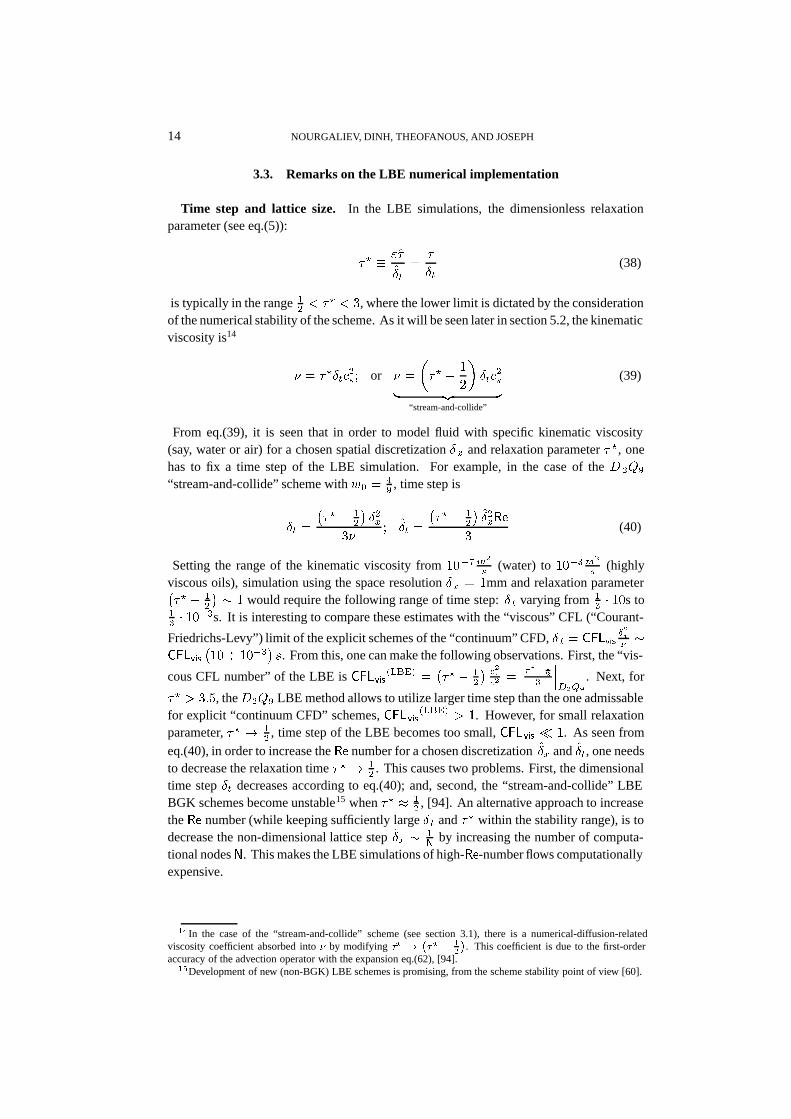
Time step and lattice size. In the LBE simulations, the dimensionless relaxationparameter (see eq.(5)):
�� � ���
���
�
�(38)
is typically in the range �� ' �� ' �, where the lower limit is dictated by the consideration
of the numerical stability of the scheme. As it will be seen later in section 5.2, the kinematicviscosity is14
� � ������� or � �
��� � �
���
��� �� �
“stream-and-collide”
(39)
From eq.(39), it is seen that in order to model fluid with specific kinematic viscosity(say, water or air) for a chosen spatial discretization � and relaxation parameter � �, onehas to fix a time step of the LBE simulation. For example, in the case of the � �(�
“stream-and-collide” scheme with )� � �� , time step is
� �
��� � �
�
���
��� �� �
��� � �
�
������
�(40)
Setting the range of the kinematic viscosity from ������
� (water) to ������
� (highlyviscous oils), simulation using the space resolution � � �mm and relaxation parameter��� � �
�
� � � would require the following range of time step: Æ � varying from �� � ��s to
�� � ����s. It is interesting to compare these estimates with the “viscous” CFL (“Courant-
Friedrichs-Levy”) limit of the explicit schemes of the “continuum” CFD, Æ � � � ��Æ��� �
� ��
���� ����
�*. From this, one can make the following observations. First, the “vis-
cous CFL number” of the LBE is � ������� �
��� � �
�
� ����� �
��� ��
�
���$�%�
. Next, for
�� + ���, the ��(� LBE method allows to utilize larger time step than the one admissablefor explicit “continuum CFD” schemes, � ��
����� + �. However, for small relaxationparameter, � � � �
� , time step of the LBE becomes too small, � �� � �. As seen from
eq.(40), in order to increase the �� number for a chosen discretization �� and ��, one needsto decrease the relaxation time � � � �
� . This causes two problems. First, the dimensionaltime step Æ� decreases according to eq.(40); and, second, the “stream-and-collide” LBEBGK schemes become unstable15 when �� � �
� , [94]. An alternative approach to increasethe �� number (while keeping sufficiently large Æ � and �� within the stability range), is todecrease the non-dimensional lattice step �Æ� � �
�by increasing the number of computa-
tional nodes�. This makes the LBE simulations of high-��-number flows computationallyexpensive.
��In the case of the “stream-and-collide” scheme (see section 3.1), there is a numerical-diffusion-relatedviscosity coefficient absorbed into � by modifying �� �
��� � �
�
�. This coefficient is due to the first-order
accuracy of the advection operator with the expansion eq.(62), [94].��Development of new (non-BGK) LBE schemes is promising, from the scheme stability point of view [60].

THE LBE: THEORETICAL INTERPRETATION, NUMERICS AND IMPLICATIONS 15
Requirements for acoustics.Simulation of compressible fluid flows using the isother-mal LBGK model is not practical. To adequately represent the sound speed in air(�� ������� �
�,�� � ����� and ���� � ������
� ), considered as an ideal gas, atime step � � �
���� �� ����
� ����* would be required for the ��(� “stream-and-collide”
LBGK scheme (with��� � �
�
�� ���� to ensure the numerical stability). The correspond-
ing grid size is � ������ � �-.. Similar estimates for water16 (�� � ������ and
�&�� � ������
� ) yield � � �����* and � � ��$..
Remark 3:
Direct counterpart of the LBE method in “traditional” CFD is the Chorin’s method of artificialcompressibility [20]. In this approach, the governing equations of viscous incompressible fluiddynamics are substituted by the following system of equation:
The method ofArtificial
Compressibility(AC)
��'��� '������� �
'��� � '����� � ���
����� �'� �'��� � '��� � � (�
" �Æ
: Artificial equation of state(41)
where���� is the density of the modeled incompressible fluid; � is the artificial density; Æ ����
is the artificial compressibility; and �� is the artificial sound speed. One can also introduce the
artificial Mach number, defined as � ��
��, where �� is a characteristic velocity scale. As can
be seen later (section 5.2), this set of governing equations is essentially the same as that of theLBE method, except that there are no artifact terms present and there exist a greater flexibility tovary fluid viscosity. Recent development of the Chorin’s AC method is a “Numerical AcousticRelaxation” (NAR) method, [75]. In [75], one can find more about comparison of the LBE andNAR.
4. LATTICE BOLTZMANN MODELS FOR HYDRODYNAMICS OFCOMPLEX FLUIDS
In the present section, a comprehensive review and critical analysis of all major LBE-based methods for modeling of complex fluid behavior are presented. We start with generalremarks on the “LBE hydrodynamics”, section 4.1. Then, most commonly used LBEmodels for complex fluids are described in sections 4.2-4.6. Finally, “pros” and “cons” ofthe LBE modeling framework for simulation of multiphase flows and complex fluids arediscussed in details in section 4.7.
4.1. General remarks
Modeling of incompressible fluids.As it can be seen from the discussion in section 3.3,due to severe limitations on time step and grid size, the LBE method is practically limitedto the modeling of incompressible low-��-number fluids.
Modeling of thermal flows. Modeling of the ‘complete’ set of transport equations(mass, momentum, energy) using the discrete kinetic approach has met with significantdifficulties. There are three major ‘plagues’ of the LBGK thermohydrodynamics. First, thethermal LBGK models are limited to /� � �
� due to a single relaxation time [3]. Second,the thermal LBGK models have severe limitations on allowable variations of temperature
��Importantly, water cannot be considered as an “ideal gas” due to the “stiff” pressure-density relation,� � ����� .

16 NOURGALIEV, DINH, THEOFANOUS, AND JOSEPH
and velocity due to the limited set of the discrete particle velocities. Third, the ‘thermal’LBGK models are prone to numerical instabilities due to ‘large stencil’ of discrete ve-locities, required to recover correct macroscopic equations; [50] [10] [71] [95] [72] [36].For these reasons, the thermal LBGK models were found inferior to a“continuum CFD”finite-difference methods ([72]) in computational time, memory requirement and stability.In practice, energy transport and phase transition cannot be modeled with the existing LBEmodels and technology17. Thereafter, we will limit our consideration to the “isothermal”LBE models.
Modeling of thermodynamic behavior. Several LBE models were developed to accountfor “non-ideality”, external forcing, and different phenomena associated with intermolecu-lar interactions. Extension of the LBE method to nonuniform (non-ideal) gases, and moregenerally to fluid-fluid multiphase flows, is accomplished either heuristically (by applyingcertain rules which “mimic” complex-fluid behaviour); or based on the Enskog’s extensionof the Boltzmann’s theory to dense gases, with incorporation of the phenomenologicalmodels of quasilocal equilibrium constant-temperature thermodynamics; and using theLBE methodology to couple the later one to the hydrodynamics of complex fluid. Themajor challenge is to accurately describe the physical mechanisms that govern the interfaceevolution (transport, breakup and coalescence). The chief difficulty is related to the break-down of the continuum mechanics theory at the fluid interfaces, where material propertiesexperience drastic changes. Considering interfaces, one naturally and intuitively thinks interms of molecules of different kind, interacting over very short distance across the inter-faces. Thus, intuitively, the models operating with the concept of particles and moleculesshould have methodological advantages over the methods of the ‘continuum mechanics’.
Modeling of particulate suspensions in incompressible fluids.The LBE method hasbeen successfully applied to particulate suspensions in incompressible fluids, a class ofproblems with complex geometry and moving boundaries. The key here is to accuratelyaccount for the momentum transfer across the solid-fluid boundary while conserving mass.In general, there are two basic LBE formulations ([58],[59], [1] and [2]) for this class ofproblems.
In the first approach ([58] and [59]), the fluid occupies the entire computational domainwith the solid particles occupied with ’interior’ fluid, eliminating the solid-fluid interfaceas far as mass conservation is concerned. This approach gives accurate results as long asthe time scale based on the kinematic viscosity of the interior fluid is sufficiently smalland the contribution of the inertia of the interior fluid is accounted for when computing theinertia of the particle. This formulation can be used only when the solid density is largerthan the fluid density.
The second approach ([1] and [2]) considers the solid particle without the interior fluidand, therefore, applies to any solid to fluid density ratio. The LBE based simulations ofsuspended particles give results [2] in good agreement with the finite element solutionsof the Navier-Stokes equations [30] for low to moderate particle Reynolds number. It is
��Recent studies of non-BGK LBE & implicit LBE models might lead to the progress in this direction [60].

THE LBE: THEORETICAL INTERPRETATION, NUMERICS AND IMPLICATIONS 17
shown [23] that this method, when applied with care, can produce very accurate particletrajectories over very long time periods, making it possible to investigate the dynamics andstability of particle motion, even near points of bifurcation. By analysis of the appropriatephase-space trajectories near transition points, the LBE method has been useful in revealingthe type of bifurcation and the scaling laws governing the particle motion [23].
4.2. Enskog extension to dense gases
In real (‘dense’, ‘non-ideal’) gases, the mean free path is comparable with moleculardimensions. Thus, additional mechanisms for momentum and energy transfer must beconsidered. Beside the transfer of molecular properties between collisions, a transferduring the collision events must be accounted for [15]. This collisional transfer hasbeen considered by Enskog (1921) [27], who approximated the effect of the exclusionvolume of the molecules under constant temperature conditions by explicitly adding the‘exclusion volume’ term into the Boltzmann collision integral. The most commonly used(approximate) form of this term is
�����coll, Enskog � �����coll, Boltzmann � � eq� 0��� �� � ���� �0�� �� �
Approximation ofthe Enskog’s
‘exclusion volume’term
(42)
where � � �)��� is the second virial coefficient in the virial equation of state; 0 is the
increase in collision probability due to the increase in fluid density, which has the followingasymptotic form [15]:
0 � � ��
�� � ������� �� � �������� �� � ��� (43)
and � and . are the diameter and mass of the molecules, respectively. Combination ofeqs.(1), (2) and (42), known as the ‘Enskog equation’ in the literature [39], was adoptedby Luo in an attempt to develop a ‘unified theory of lattice Boltzmann models for nonidealgases’18, [66].
It is instructive to note that, in his derivation, Enskog employed a ‘hard-sphere model’,which has the advantage of mathematical simplicity, since many-body interactions areneglected (collisions are instantaneous). This model is, however, not appropriate for realgases under high pressure, because the molecules are in the force field of others during alarge part of their motion, and multiple encounters are not rare 19, [15].
�Luo employed the BGK collision operator multiplied by �, �����coll, Boltzmann � ����eq�
.
��Enskog’s preference of the ‘hard-sphere model’ rooted in the belief that molecular chaos is valid for rigidspherical molecules even at high gas densities. This assumption is accurate only for uniform steady state [15],while for non-uniform state (for example, in the regions of fluid-solid boundaries and fluid-gas interfaces),correlation between velocities of neighboring molecules may exist due to a memory effect.

18 NOURGALIEV, DINH, THEOFANOUS, AND JOSEPH
4.3. He, Shan and Doolen extension to dense gases
He, Shan and Doolen (1998) [44] proposed the following approximate model of densegases. The starting point was the LBGK equation in the form20:
��� � � � ��� � �� � � eq
��
��� �� � ��� ��
���� eq (44)
where � and � are the effective molecular interaction and gravity forces, respectively,� � ���
� . The effective molecular interaction force � is designed to simulate non-idealgas effects.
� � � ��� �� �Intermolecular attraction
by mean-fieldapproximation
� � ����0 � ���� �0�� �� �
Enskog’s exclusion volume effect of themolecules on the equilibrium properties
of dense gases
(45)
The intermolecular attraction potential21 � is expressed as
����� �
�!��*�
�attr����� ���� ��� (46)
where �attr����� is the attractive component of the intermolecular pairwise potential ofmolecules ‘0’ and ‘1’ separated by distance ��� � ��� � ���. The next step is to expanddensity about ��. Assuming that density gradients are small, the intermolecular attractionpotential is expressed as
� � �� � 1�� (47)
where constants � and 1 are given by
� � ��
�!*�
�attr��� ��� 1 � ��
�
�!*�
���attr��� �� (48)
with 1 determining the strength of the surface tension. Elucidating the thermodynamicalaspects of this model, the intermolecular force � can be cast into the following form [40]:
� � ��/ � � 1 ��� � �� �Force associated
with surface tension
/ �� � � � ����0� � � � / � ��
�� �� �‘Non-ideal part’ of
the equation of state
� / � ����� � � 0�� � � (49)
��Here, we would like again to note the conceptual difficulty with interpretation of the “LBE’s molecules”, dueto the definition of sound speed by eq.(14) (see Remark 1).
��Implementation of the intermolecular attraction potential � allows to effectively compensate for certainlimitations of the Enskog ‘hard-sphere’ model.

THE LBE: THEORETICAL INTERPRETATION, NUMERICS AND IMPLICATIONS 19
Setting � � +���+ , the van der Waals equation of state is obtained22:
/ � ���
�� � � � � (50)
4.4. Free-energy-based models
Swift et al. ([96] and [97]) developed a model for non-ideal fluids to account forthe interfacial thermodynamics. The general idea is to incorporate phenomenologicalapproaches of interface dynamics, such as Cahn-Hilliard and Ginzburg-Landau models,using the concepts of free-energy functional; and to utilize the discrete kinetic approach asa vehicle for coupling with complex-fluid hydrodynamics. The pressure tensor is definedusing the Cahn-Hilliard’s approach for non-equilibrium thermodynamics. Strictly speaking,this model is phenomenological, in which the thermodynamic effects are introduced througha phenomenological equation of state. The term ‘free-energy-based’ is attributed to themodel chosen for pressure tensor eq.(51) [13].
���� �� �
�/� � 1 ��
� �1
��� �
� Æ �� � 1� � �� (51)
Thermodynamical pressure /� can be given by, e.g., van der Waals equation, eq.(50).Parameter 1 is a measure of the interface free energy. For flat interfaces, 1 is related to thecoefficient of surface tension through the equation:
1 �� �
'�'�
��
�$(52)
where $ is the normal-to-interface direction.
Multi-component versions of the free-energy-based model were developed in [97] and [62].
4.5. Interparticle interaction potential model of Shan and Chen
One of the first LBE model for multiphase flow is due to Shan and Chen [90] [91] [92][93]. In this model, an additional momentum forcing term is explicitly added to the velocityfield after each time step:
����� �� � ���� �� � 2���� �� where (53)
2���� �� � ��
����
���
������ �����
where � is a “potential” function and � is a “strength” of the interparticle interaction.The ’corrected’ velocity �� is employed in the equilibrium distribution function, givenby eq.(B.9). By introducing an additional forcing term, this model effectively mimics the
��Other equations of state can be implemented in a similar way.

20 NOURGALIEV, DINH, THEOFANOUS, AND JOSEPH
intermolecular interactions (‘complex fluid behaviour’). Although it is possible to show thatthe total momentum in the whole computational domain is conserved [91], the momentumis not conserved locally. As a result, a spurious velocity always exists in regions adjacent tothe interface, Fig. 2. The forcing term 2� in eq.(53) corresponds to the following non-localpotential function
������� � ������� ���� ����� (54)
0.5 0.6 0.7 0.8 0.9 1r
10−6
10−5
10−4
10−3
10−2
10−1
|usp
urio
us|
Free−energy−based modelShan and Chen model
"Physically−Diffuse Interface"
LIQUID
GAS
FIG. 2. Velocity distribution across the interface for the “Shan-Chen” and “Free-energy-based” models.Bubble of the van der Waals fluid at equilibrium, [74].
One can avoid the step eq.(53) by directly substituting� � into the equilibrium distributionfunction eq.(B.9). Effectively, this means addition of the following “correction” term tothe equilibrium distribution function [74]:
���� � ���
� � ��� � � � �� ��� � (55)
��� �
�� )�
����� ����
����
�� � �
��
and
����� � )�
���� � � � � ��
�� �
���������������
�� �� � ��� �
� ��
�

THE LBE: THEORETICAL INTERPRETATION, NUMERICS AND IMPLICATIONS 21
4.6. He, Chen and Zhang model
He et al. (1999) [40] extended the HSD model to incompressible multiphase flow. Twosets of distribution function are utilized. The first one is used to “capture” incompressiblefluid’s pressure and velocity fields, using the concept of “artificial compressibility” [41].Another discrete distribution function #� is introduced with the sole purpose to “capture”the interface; which makes this approach close in spirit to the “continuum CFD” methodsfor interface capturing - the “level set” and “volume-of-fluid” approaches. After each timestep, the “index” function 3 �
�� #� is re-constructed, allowing to enforce a smooth
transition of densities and viscosities at the “numerically smeared” interface:
�3� � � � ,�,�,��,� � � � ��
� �3� � �� � ,�,�,��,� ��� � ���
(56)
where �, �, �� and �� are density and kinematic viscosity of the two fluids; and 3�, 3�
are the minimum and maximum values of the ‘index’ function, respectively.
4.7. Assessment of the LBE modeling framework for multiphase flow and complexfluids
Since the lattice Boltzmann equation method is a particle method, it is argued that, forsimulation of interfacial phenomena, the LBE method has potential to be superior compar-ing to the “continuum” CFD methods [90] [91] [92] [93] [96] [97] [102]. In the presentsection, we will address the question whether, why and when the LBE approach may beadvantageous for simulation of the interfacial phenomena. It is important to realize thatthe computational modeling of multiphase flows is not open for ‘purism’. That is, thereare no ‘universal models’ able to perfectly work under any flow conditions. One has tobe aware of the limitations and advantages of the approach chosen, since every one has itsown domain of applicability. In Appendix C, we provide a classification of the moderncomputational methods for fluid-fluid multiphase flows, which would enable us to properlyappreciate the perspectives of the discrete kinetic approach.
To discuss the LBE method for multiphase flows, we have chosen three most successfuland popular LBE models: the ‘Shan-Chen’ (‘SC’) model (section 4.7.1); the ‘free-energy-based’ model (section 4.7.2); and the ‘He-Shan-Doolen’ (‘HSD’) model (section 4.7.3).The other multiphase LBE models are due to Gunsteinsten at al. [38] and Luo [66].
4.7.1. ‘Shan-Chen model
The ‘SC’ LBE method [90] [91] [92] [93] has been quite successful in simulation of sev-eral fundamental interfacial phenomena,such as, e.g., Laplace law for static droplets/bubblesand oscillation of a capillary wave (see for review [16]). However, there are a few limita-tions of the ‘SC’ model, which make this method inferior in comparison to other methodsfor multiphase flows.
The first serious problem is that one cannot introduce temperature which is consistentwith thermodynamics. It is possible to show that the ‘SC’ model has the following equation

22 NOURGALIEV, DINH, THEOFANOUS, AND JOSEPH
of state [91]:
/ � ��� �
����
��� �� �� �"�
(57)
where � � � and � for a ��(� lattice. Suppose we would like to study fluid withthe ‘non-ideal’ part of the equation of state / �. In order to reproduce this equation of state,the following � function must be utilized:
�� � �
� / �
���� � / � � / � ��� (58)
It is possible to show, that the Maxwell’s “equal-area” reconstruction is possible onlyfor one special form of the potential function, � � �� ���� �� �, where �� and �
are arbitrary constants [91]. The role of temperature in this model is effectively takenby the strength of the interparticle interactions �. By varying �, one could construct�� � �-diagram, which mimics the �� � �-diagram, Fig. 3.
0.10 0.12 0.14 0.16 0.18|G|
−0.5
0.0
0.5
1.0
1.5
2.0
2.5
3.0
∆ρ
G =-1/9
b)
c
G=-0.18a)
FIG. 3. a) �� ���-diagram for the ‘SC’ model (� � ����� ����), demonstrating the occurrence of thefirst-order phase transition at the analytically predicted “critical” strength of interparticle interactions, �� � �
�,
[86]. b) Typical density distribution at the state, close to the equilibrium.
The next problem is related to the way this model represents capillary effects, whichcan be quantified by the coefficient of surface tension . It can be shown, that for the ‘SC’model, in the case of the flat interface, the coefficient of surface tension can be calculatedfrom the following equation [91]:
���
�
� ��
��
�/ � � �
��/ �
�$��$ (59)
where $ is a direction normal to the interface. This means that is coupled to the equationof state through / � and there is no freedom to vary it. Typically, for a chosen potentialfunction and “strength of interparticle interactions�”, the surface tension of the “SC” modelis “empirically” determined by generating circular bubbles/droplets of different radia in a

THE LBE: THEORETICAL INTERPRETATION, NUMERICS AND IMPLICATIONS 23
periodic domain, and estimating the slope of the “pressure-difference vs. inverse of radius”relation (Laplace law, Fig.4), [104], [86].
Another severe limitation is related to the inability to represent different viscosities indifferent phases. All LBE simulations of multiphase flows performed to date have assumedthat all phases or components of the multiphase system possess the same kinematic (�) and“second” ( -� ) viscosities, defined by the relaxation time23 � and lattice geometry, eq.(84).
In our classification of the CFD methods for multiphase flows, Appendix C, the ‘SC’model belongs to the class of “physically-diffuse-interface” methods. These methods donot require to “track” or “capture” the interface position, since the “phase separation” and“interface sharpening” mechanisms are provided by the momentum forcing term 2�. Effec-tively, 2� plays the role of both the Korteweg’s capillary stress tensor and the “non-ideal”part of the equation of state / �. The ‘SC’ method builds the interface physical model basedon the continuum variable : 2� � � � � �� ��. There is no direct use of the one-particleprobability distribution function, �� - a distinct feature of the LBE method.
4.7.2. “Free-energy-based” model by Swift et al.
The free-energy-based LBE approach has been applied to several physical phenomenain binary and ternary fluids, such as flow patterns in lamellar fluids subjected to shear flow[34]; effect of shear on droplet phase in binary mixtures [102]; spontaneous emulsificationof droplet phase in ternary fluid, which mimics the oil-water-surfactant systems [62]; etc.
The main advantage of this model over the ‘SC’ LBE method is that it was formulatedto account for equilibrium thermodynamics of non-ideal and multi-component fluids at afixed temperature, allowing thus to introduce well-defined temperature and thermodynam-ics. The model is, therefore, consistent with the “Maxwell’s equal-area reconstruction”procedure, Fig.5.
Furthermore, since the model admits local momentum conservation, the interfacial spuriousvelocity is nearly eliminated [74], Fig.2.
Similar to the ’SC‘ model, the free-energy-based models do not utilize the ‘particle’ natureof the discrete kinetic approach. The major drawback of this approach is that the modelsuffers from unphysical Galilean invariance effects, coming from the ‘non-Navier-Stokes’terms, which appear at the level of the Chapman-Enskog analysis of the discrete Boltzmannequation (see section 5.4 and Appendix E). Efforts are being made to reduce this unphysicaleffect [48].
��One possible way to vary viscosity is to introduce spatially-variable relaxation time, which allows variableviscosity in the ‘bulk’ region of different fluids [67]. Effect of this approach on dynamics of interface has yet tobe investigated.

24 NOURGALIEV, DINH, THEOFANOUS, AND JOSEPH
0 0.01 0.02 0.03 0.04 0.05 0.06 0.071/rb
0
0.0002
0.0004
0.0006
0.0008
0.001∆P
Free−energy−based model, κ=0.015 (100x100)T/D definition, Free−energy−based model, κ=0.015Free−energy−based model, κ=0.037 (100x100)Free−energy−based model, κ=0.037 (200x200)T/D definition, Free−energy−based model, κ=0.037Shan−Chen model (100x100)
FIG. 4. Laplace law for the “SC” and the “free-energy-based” models: � as a function of ���
(� is aradius of the generated bubble) for a van der Waals fluid. Solid and dashed lines are the results from the “flatinterface test”, with thermodynamical definition of surface tension by eq.(52), [74].
4.7.3. He, Shan and Doolen model
This model was developed [44] as a revision of the ‘SC’ model. In difference to the‘SC’ model, the ‘HSD’ model is linked to the kinetic theory of dense gases, section 2.1.The intermolecular interactions are formulated using the approximation of the Enskog ex-tension of the Boltzmann equation. As a result, the ‘HSD’ approach is more flexible forimplementation of the thermodynamical model, with the “consistent” temperature concept,admitting the correct Maxwell’s “equal-area” reconstruction procedure. The capillary ef-fects are modeled by the explicit implementation of the “density gradient model”, 1�� � ,eq.(49), allowing flexibility in variation of the coefficient of surface tension by varying theparameter 1.
The serious limitation of the “HSD” model is related to the numerical instability, asso-ciated with the ‘stiffness’ of the collision operator, when the ‘complex fluid’ effects areintroduced through the ‘forcing’ term, eq.(49). These stability problems might be alleviatedby providing ‘robust’ numerical schemes for advection and collision operators, like thosediscussed in section 3.2.2 and ref. [98].
The two-component version of the ‘HSD’ model (“He-Chen-Zhang extension”, see sec-tion 4.6) is close in spirit to the “front capturing” methods of the ‘NDIA’ (see Appendix

THE LBE: THEORETICAL INTERPRETATION, NUMERICS AND IMPLICATIONS 25
0.4 0.9 1.4 1.9 2.4 2.9 3.4ρ
0.39
0.41
0.43
0.45
0.47
0.49
0.51
0.53
0.55
0.57R
T
Maxwell reconstruction Free−energy−based model Shan−Chen model
RTc
gas
gas+liquid
FIG. 5. Coexistence curve (gas branch), calculated by the “SC” and the “free-energy-based” models, [74].Van der Waals fluid. �� is a “critical temperature”.
C), where the “index” function 3 eq.(56) effectively plays the role of the ‘volume-of-fluid’or the ‘level set’ functions. In [40], this model has been used to simulate Rayleigh-Taylor instability. The results of the simulation are comparable with those obtained bythe “continuum” CFD approaches, using the “VOF”, the “Level Set” and Tryggvason’s“front-tracking” methods. Fig.6 shows comparison of the HSD LBE model with the pseu-docompressible NAR method, [75]. The later utilizes the level set function approach for“capturing” interface24. While being able to describe basic numerical tests for multiphaseflows with accuracy comparable to the LBE method (e.g., single-mode Rayleigh-Taylorinstability, Fig.6), the NAR approach offers important flexibility currently not available inLBE. For example, implementation of variable fluid viscosity and heat transfer is straight-forward. Perhaps more importantly, in NAR we have no constraints on the density ratio ofthe fluids across an interface, as applicable in all low-pressure liquid-gas systems. This isdemonstrated by the dam-breaking problem (density ratio 1:1000) in Fig.7.
��The “Numerical Acoustic Relaxation” (“NAR”) method is devised from the classical concept of “artificialcompressibility” due to Chorin and combined with a ghost-fluid methodology and level-set algorithm for interfacecapturing and robust treatment of phase coupling. High accuracy and computational efficiency of the method areachieved by using a characteristics-based conservative finite-difference approach and introducing a generalized“time-stretching” scheme to solve the hyperbolic conservation laws. For details of implementation and validationsee [75].

26 NOURGALIEV, DINH, THEOFANOUS, AND JOSEPH
t=0.0 t=1.5 t=2.0
NAR
LBE
FIG. 6. Rayleigh-Taylor instability. Comparison of the “Level Set-NAR” [75] and the HSD-LBE [40]methods. Parameters of the test-case (“Level Set-NAR”/“HSD-LBE”): �� � ���; �� � ���; single-modeinitial perturbation with amplitude ��; grid resolution - � �� ���
���� � ��� ����
���. The “upper”
fluid has density � � �; while the “lower” fluid has density � � .
4.7.4. Summary
On one hand, the LBE methods for fluid-fluid multiphase flows are able to reproduceseveral basic interfacial phenomena, such as spinoidal decomposition in binary fluids, os-cillation of a capillary wave, Rayleigh-Taylor instability, etc., with the results comparable

THE LBE: THEORETICAL INTERPRETATION, NUMERICS AND IMPLICATIONS 27
t=0.05 sec
t=0.10 sec
t=0.15 sec
t=0.25 sec
t=0.30 sec
t=0.20 sec
FIG. 7. Collapse of water column in a rectangular box using the “Level Set-NAR” approach. Density ratiois 1:1000. Dimensions of the water column and box are � and �� ��, respectively. =14.6 cm.
to those obtained by the methods of the “continuum” CFD. On the other hand, the currentlyexisting multiphase LBE methods are not able to beneficially utilize the ‘kinetic theoryorigin’ of the method. That is, in order to simulate the interfacial phenomena, all currentlyexisting LBE models practically employ the same techniques, as those used in the “contin-uum” CFD: i.e., intermolecular interactions are implemented through the phenomenologicalthermodynamical models - equations of state; and the capillary effects are introduced byutilizing the “density gradient” approaches. Additionally, there are challenges to overcomein order to demonstrate the LBE scheme as a competitive methodology, comparing to thedirect solution of the conservation equations of continuum mechanics. These include aconsistent modeling of energy transport; elimination of excessive numerical discretizationerrors; and robustness and numerical stability under wide range of flow conditions andmultiphase flow properties.

28 NOURGALIEV, DINH, THEOFANOUS, AND JOSEPH
5. DERIVATION AND ANALYSIS OF THE CONTINUUM EQUIVALENT OFTHE LB EQUATION
In the present section, we outline the major steps of the Chapman-Enskog expansionmethod, applied to the LBE BGK method, deriving the successive hierarchy of the LBGKequations, section 5.1. Then, the equations of hydrodynamics are derived and analyzed insections 5.2-5.4.
5.1. Chapman-Enskog expansion method
The purpose of the Chapman-Enskog method is to solve Boltzmann equation by suc-cessive approximations. This shall yield solutions, that depend on time implicitly throughthe local density, velocity and temperature, ���� � � ��������� � ��� � - the ‘Chapman-Enskog ansatz’, [49]. In the present section, we outline the basic steps of the procedure,applied to the isothermal discrete Boltzmann equation (28).
First, we introduce a formal expansion of the discrete probability distribution function:
�� � � ���� � �� ���
� � ��� ���� � ��� �
����
��� ���� (60)
where � is a lattice Knudsen number, eq.(26), which keeps track of the order of the terms inthe series. The Chapman-Enskog expansion provides a consistent and practical definitionof � ���
� [49]. The functions � ���� are defined in such a way so that � ���
� decreases as �increases. To satisfy eqs.(21), the first three moments of the zeroth approximation shallreproduce macroscopic density, velocity and kinetic energy, while corresponding momentsof the higher-order terms are set to zero:�
� ����� � �
�� �
���� ��� � �
��
�� �
���� � ���� � � �
�� � ��
� ����� � ��
�� �
���� ��� � ��
�� �
���� ��
� � �� $ + �(61)
LBE conservation laws. Substituting expansion eq.(60) into eq.(28) 25 and taking thefirst ‘discrete moment’ �
�� eq.(28)� result in the mass conservation equation
Mass conservation law:�� � �� �� � �
(63)
Taking the second ‘discrete moment’ ��
� eq.(28) ���� yields the momentum conserva-tion law:
�� � � �������
����
����������� �
�����
���
���� ������ � � ��
�(64)
��To avoid using expansions:
����� ���� � �� ������
��
���� ����� �� � � ��� � �� � � (62)
traditionally employed to evaluate the ‘stream-and-collide’ advection operator,��� � � �������Æ�� �Æ�������� �, [41] [96], we assume that high-order finite-difference scheme is applied to the��� � � ������������(see section 3).
THE LBE: THEORETICAL INTERPRETATION, NUMERICS AND IMPLICATIONS 29
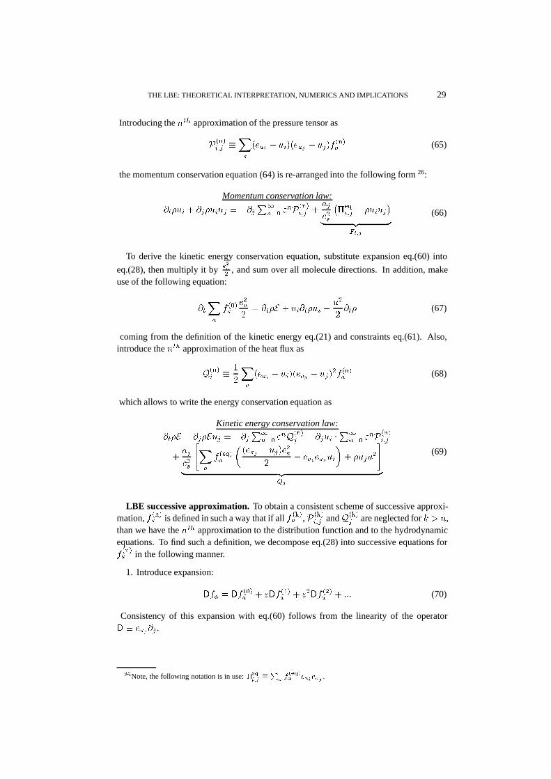
Introducing the $�� approximation of the pressure tensor as
���� �� �
��
���� � � ����� � �������� (65)
the momentum conservation equation (64) is re-arranged into the following form 26:
Momentum conservation law:
�� � � �� � �� � �����
�� ������
�� ������
���� �� � � ��
�� �� �
.� �
(66)
To derive the kinetic energy conservation equation, substitute expansion eq.(60) into
eq.(28), then multiply it by ���� , and sum over all molecule directions. In addition, make
use of the following equation:
����
� ����
���
� �� � � � �� � � ��
�� (67)
coming from the definition of the kinetic energy eq.(21) and constraints eq.(61). Also,introduce the $�� approximation of the heat flux as
���� � �
��
���� � � ����� � ����� ���� (68)
which allows to write the energy conservation equation as
Kinetic energy conservation law:
�� � � �� ��� � �����
�� ������
� � ��� ���
�� ������
��
������
���
� �����
����� � ����
��
� �������
�� ���
�
�� �� �
%�
(69)
LBE successive approximation.To obtain a consistent scheme of successive approxi-mation, � ���
� is defined in such a way that if all � ���� , ����
�� and ����� are neglected for � + $,
than we have the $�� approximation to the distribution function and to the hydrodynamicequations. To find such a definition, we decompose eq.(28) into successive equations for�
���� in the following manner.
1. Introduce expansion:
�� � � ���� � � � ���
� � �� � ���
� � ��� (70)
Consistency of this expansion with eq.(60) follows from the linearity of the operator � ����� .
��Note, the following notation is in use: ������ ��
� ����� ������ .

30 NOURGALIEV, DINH, THEOFANOUS, AND JOSEPH
2. Consider ����. Due to the ‘Chapman-Enskog ansatz’, �� depends on time implicitly,only through the , � and � . Thus,
�����
�����
�
���
���� �
� � ��
����� �
� ���
(71)
To expand eq.(71) into infinite series in powers of �, expand '��'� , '��
'���and '��
'�� as
'��'� �
'� ���
'� ��'� ���
'� ��� '����
'� � ���'��'���
�'� ���
'�����
'� ���
'������ '�
���
'���� ���
'��'�� �
'� ���
'�� ��'� ���
'�� ��� '����
'�� � ���
(72)
The expansions for time derivatives �� , �� � and �� � must be defined to be consistentwith the conservation laws eqs.(63), (66) and (69). Thus, the definition of '�
'� is taken fromthe $�� approximation to the conservation laws:
Mass conservation:��� � ��� ����� � �� �$ + ��
(73)
Momentum conservation:
��� � � ��� � �� � ������ �� � 4 ��
��� � � ������� �� � �$ + ��
(74)
Energy conservation:
��� � � ��� ��� � ������� � ��� � ����
�� �(�
��� � � �������� � ��� � ����
�� � �$ + ��
(75)
As a result, the following consistent expansion of �� is obtained27:
�� � ��� � ���� � ����� � ��� (77)
3. With the defined expansions (60), (70) and (77), the LBE transport equation (28) canbe written as28:��
��� � ���� � ����� � ����� � �
����� � ��
���� � ���
���� � ���
��
� � �#�
���
���� � ��
���� � ���
���� � ���
�� ���
�
�
�����
���� � �������
(78)
��This formulation differs from [3] and [17], where the time derivative is expanded as
�� � ���� � ����� � ��� (76)
�Note, ���� is omitted.

THE LBE: THEORETICAL INTERPRETATION, NUMERICS AND IMPLICATIONS 31
4. To uniquely define ����� we require that the coefficient of each power of � vanish
separately in eq.(78). Thus, the equations to be solved to yield all the � ���� are
Successive hierarchy of the LBGK equations:
����
�� �
��� � ����
0��-order: “Euler”
����
� ������� � �
��� � �
���
������
���� � �������
1��-order: “Navier-Stokes”
��� ���High-order: “Burnett”, “Super-Burnett”, etc.
��� �������
� ������� � ����
����� � ���� ����
��� ��
��� � �
�����
��� ���
(79)
In the Chapman-Enskog theory for the Boltzmann equation, in order to reproduce theNavier-Stokes equations, only the first two approximations � ���
� and � ���� are required29.
In the following section, we recover and analyze the equations of hydrodynamics corre-sponding to three most commonly used isothermal LBE models.
5.2. Hydrodynamic equations of the ‘ideal fluid’ LBGK model
Navier-Stokes equations. The governing equations of the compressible isothermalNewtonian fluid hydrodynamics are [63]
�� � �� �� � �
�� � � �� � �� � �� / � ��� �� � � (80)
where the viscous stress tensor has the following form [5] :
� �� � 5 ���� � � ��� �
�6 �
�5
�� �� �
‘Bulk’ viscosity, �
���� � Æ �� (81)
and 5 and 6 are the ‘first’ and the ‘second’ fluid viscosities. Following Stokes, the ‘bulk’and ‘second’ viscosities are � � � �
�5 and 6 � �, respectively, [5].
��There exist fundamental difficulties when truncations of the Chapman-Enskog expansion are used beyond
the Navier-Stokes order ���� , (‘Burnett-’ and ‘super-Burnett’ equations level). Notably, any truncation beyond
���� is inconsistent with the Clausius-Duhem inequality, which is often taken as a representation of the second
law of thermodynamics [89]. This fact was first noted for compressible gas dynamics by Bobylev [9] and later byLuk’shin [65]. Although the modifications of Navier-Stokes equations due to Burnett were expected to provideresults superior to that of Navier-Stokes equations under high �� numbers, present evidences indicate that thisis not so; in fact, where the Navier-Stokes equations are themselves perhaps not completely adequate, the higher-order equations may even be inferior. Since the expansion eq.(60) is asymptotic; when the first two terms give avery good approximation, the third term may provide a further refinement. However, when the first two terms fail,inclusion of higher-order terms likely make matters worse; this is a known behavior in asymptotic series [33].

32 NOURGALIEV, DINH, THEOFANOUS, AND JOSEPH
LBGK hydrodynamic equations30�31. For the case of the “ideal-gas LBGK model”,the pressure tensor is given by
����� �� � � ���
� � Æ �� (82)
Since the “zeroth-order solution of the LBGK equation”, eq.(79), is ������ � ��
����� , the
momentum flux tensor is ����� �� � ��
���� �� . Thus, the momentum conservation equation (66),
which is the “first-order solution of the LBGK equation”, eq.(79), is:
���� �� � ��� � �� ��� � ��� � ���� � ���
� !
� ����� ��� �� �
Viscous stresstensor,� �� ����
� �
"#######$
� � �� (83)
Viscosity. The ‘first’ and the ‘second’ viscosities are defined as32
�5 � ���� ���� �
�������
�� �� ����
� � �6 �
��5 (84)
which renders the following definition of the dimensional kinematic viscosity:
� � ���� (85)
An assumption of the constant temperature would require the following constraint besatisfied:
��������� � ����� � ��� � ��� �� � �����
�� � �(�
��������� � ���� �� � �����
��
(86)
For this LBGK model, the viscous stress term is (details of the derivation are given inAppendix D):
����
�� �����
��
�� ���
�� ���� �� � ���
��� �� � ��
��� ���� �� (87)
where �� �� is the non-dimensional Navier-Stokes viscous stress tensor, defined by eq.(81);��
��� ���� �� is a “non-linear33 deviation” of this LBGK model from the classical Navier-Stokes
��To avoid confusion, in the present section, we will use ���� to denote non-dimensional variables.��In the following analysis, it is assumed that the lattice geometry is chosen in such a way so that ��� � ���� .
(See appendix A for the lattice geometry).��Note, the �� is not Stokesian, �� �� �. The value of the ‘second’ viscosity is not important as long as the
velocity field is close to the ‘divergence-free’ condition of the incompressible fluid.��The term “non-linear” reflects the fact that the deviation is ‘cubic’ in velocity, � ������ .

THE LBE: THEORETICAL INTERPRETATION, NUMERICS AND IMPLICATIONS 33
equations, given by
����� ���� �� � �
�� ����
����
���� ��� ������ � �� ��� � �
��� ��������� � �����������
� ��� ���
��� ��� ������ � ����� �����
� �
� ��� �� ���
���
�� �� ��� ����#�
� (88)
where �� � ���/ � �
�� and � are the Reynolds and Froude numbers, respectively.
Thus, the governing equations of this LBGK model are
���� � ��� � ��� � �
���� �� � ��� � �� ��� � ��� �/ � ���
�
��
���� �� � �� ���
��
�
��# � �� �
Linear Part: not quite Incompressible Navier-Stokes [see eq.(E.6])
� ����� ���� ��� �� �
Non-linear deviations
(89)
where �# is a unit vector specifying the orientation of the external body force.
The deviations of the continuum equivalent of this LBE model from the incompressibleNavier-Stokes equations are detailed in Appendix E. From this, one can see the implicationof ���, the dimensionless “pseudo-sound-speed”, introduced in eq.(28). In the linear term,it leads to the kinematic viscosity and Reynolds number that appears in front of the linearpart. By appropriate choices of ��� and �� , flow with any Reynolds number (any viscosity)can be modeled by eq.(14). On the other hand, in the non-linear (“cubic”) term, we are leftwith terms that contain, in addition to ��, ���
� and ����. Thus, we can make these terms as
small as we wish by requiring that ��� is chosen so that��� ����
�� � and��� � ���
�
�� � (90)
In fact, it turns out that these conditions are automatically satisfied as long as �� � � �, andthe basic stability criterion for integration of the LBE, namely that ���
�' � are satisfied.
To see this, take � as the number of lattice points in the cross-stream direction (� � �),and suppose we chose ���
�� ��
�. We then have
�
�� ����
��������
from which it is seen that the condition ��� � � is moderate because� � �. Also, you willnote that for inertia flows, ��� �, the condition on ��� � � is moderate34, but for viscousflows, �� ' �, we must obey a stronger condition on ��� � �, so that �� ���
� � � and the“non-linear term” is smaller than the inertia “term”.
We have verified numerically that indeed, as long as these conditions and ��� � � are
satisfied, exact solutions can be obtained arbitrarily close in Poisseulle and Couette flows,
��The smallest term in the Navier-Stokes equations is of the order ���
, thus, the requirement for ��� is ���� �
������

34 NOURGALIEV, DINH, THEOFANOUS, AND JOSEPH
for any values of viscosity (or Reynolds number). Also note that, as appropriate for incom-pressible viscous flows, the pressure level is immaterial. If the pressure drop is specified, itimplies a corresponding density drop, through eq.(82), and care must be exercised, becauseerrors will be introduced unless ��
� remains much less than 1.
5.3. Hydrodynamic equations of the isothermal ‘HSD’ LBGK model for nonidealfluid
In the He-Shan-Doolen model, the pressure tensor and body force are given by
���� �� � ��
� � Æ ��4 �� � ��Æ �� � �� �
�'�"��0�'�'�����(�
�
(91)
where 7� is an acceleration due to the external body force; and the ‘non-ideal’ part of theequation of state / � is given by, e.g., van der Waals eqs.(49) and (50). The distinguishedfeature of this model is that the non-ideal equation of state (pressure) is incorporated directlythrough the momentum source term. The momentum conservation equation, written in the“dimensional” form, is:
�� � � �� �� � � � �� �
� �� � ��� �� �� �� � �
��
� 7 � �� �� �
���
��
���� ��� � / �� ��� �� �
Non-ideal gaspressure� �� �
� ��������
�
�1 � ��� � �� �
‘Capillary stress tensor’ �� �� �� �� �
��
�
��
����
� �
�
������� ��
�� �� �
Viscous stresstensor,�� ����
� �� �� �� ��� ��� �� �
� �
����
�
��
� �������� � ���������� �
(92)
where the Weber number and density variations are defined as
�� � ������
1
Æ �
� �������
���
Æ �
��
��
��
(93)
respectively; and ! are the saturation density of the liquid and vapor phase underchosen temperature � ; and �
� is a scale of the density variation over characteristic time
scale �� � �
��. In the scaling analysis of eq.(92), the temporal and spatial derivatives of the
density are estimated as
�� � ������
� � ������
� � � �������
���
� �� � �������
(94)

THE LBE: THEORETICAL INTERPRETATION, NUMERICS AND IMPLICATIONS 35
In addition, parameters 1, � and � are scaled as
1 � �1���
�����
�
����
� � �����
���
� � ���
(95)
respectively.
The ‘constant-temperature’ condition is defined by eq.(86). The viscous stress tensor� ���� �� is derived in appendix D. Choosing the lattice with ���� � ���
�, the ‘first’ and the‘second’ viscosities are defined by eq.(84).
The deviations of the continuum equivalent of this LBGK model from the incompressibleNavier-Stokes equations are detailed in Appendix E.
5.4. Hydrodynamic equations of the isothermal ‘free-energy-based‘ LBGK modelfor non-ideal fluid
The governing hydrodynamicequations of this LBGK model, written in the “dimensionalform”, are35�36:
�� � �� �� � �
�� � � �� �� � �� � Æ
��
� �� � ��� �� �� � �� � Æ
��
� � � /�� �� �� �
�Æ
�����
�� ��
��1 ��
� �1
��� �
��Æ �� � 1� � ��
� �� �
‘Capillary stress tensor’,�� � � �
�
�
����
�
�
�
�� ��� ��
�� ����� ��� �� �
Viscous stresstensor,�� ����
� �
� (96)
Derivation of the viscous stress tensor � ���� �� is similar to that one for the “isothermal37
ideal gas” model and given in appendix D:
���� ���� ��
�� ��� ��� �� �
� �
����
�
��
� ��� ���� �� � �
��� ���� �� (97)
��The body force has not been incorporated in any existing variants of this model, � � �.��In the present section, we use ���� to explicitly denote non-dimensional variables.��Even though the concept of temperature can be introduced in the pressure tensor, it causes violation of the
energy conservation in the LBE discrete kinetic theory, eq.(69) [66]. The ‘constant-temperature’ condition eq.(86)cannot be satisfied. This is a generic problem for all “isothermal” LBGK models.

36 NOURGALIEV, DINH, THEOFANOUS, AND JOSEPH
In the analysis of this model, we assumed that the lattice geometry is such, so � ��� � ����.
With this, the following viscosities are obtained:
5 � ���������
� 6 � 5
� !
�
��
�
���
� �
�� � � �
��� � ��� �� �� � ���
� 1���
���� �� �
� �
��
�
������
�
"#########$
(98)
Notably, the second viscosity is non-Stokesian38. It is also dependent on the virial coeffi-cients of the equation of state and second gradients of density.
The deviations of the continuum equivalent of this LBE model from the incompressibleNavier-Stokes equations are detailed in Appendix E.
6. COMPUTATIONAL EFFICIENCY
In what follows, we will discuss ‘pros’ and ‘cons’ of the LBE method as a ‘Navier-Stokessolver’, in terms of its simplicity, efficiency and capability for an efficient parallelization.
Simplicity. Simplicity in implementation has been used as an argument in favor ofthe LBE method. The simplest “stream-and-collide” LBE algorithm with “bounceback”boundary condition formulation is indeed easier to program and handle than the “contin-uum” CFD algorithms for solving the Navier-Stokes equations, often involving the solutionof the Poisson equation, sophisticated Riemann solvers to handle convective terms; the useof unstructured grids to accurately describe flow in complex geometry; etc. However, afair comparison would instantly eliminate the illusion about the superior simplicity of theLBE method. In fact, direct counterparts of the LBE are the “compressible flow methodsfor incompressible flows”, such as, Chorin’s approach of “artificial compressibility” (AC).This method does not require Poisson equation solvers, and it is also very simple for im-plementation on a regular mesh, [75]. Recent development of the Chorin’s AC methodis the “Numerical Acoustic Relaxation (NAR)” method. In [75], we utilized the NARfor different single- and multiphase flow problems, which include “Lid-Driven Cavity”,the “Doubly Periodical Shear Layer Flow”, “Rayleigh-Taylor Instability” and “Collapseof Water Column”, comparing it with the LBE and other methods of incompressible fluiddynamics. Based on our experience with both NAR and LBE, we have found no advantageof using discrete kinetic method over direct solution of the Navier-Stokes equations.
The elusive simplicity of the LBE approach further fades away when the LBE method ispushed to match requirements on accuracy and stability, typical for advanced CFD codesbased on solving the Navier-Stokes equations. In fact, the LBE method is by far more
�For this model, there are strong velocity divergence sources at the interface, making the second viscosityimportant.
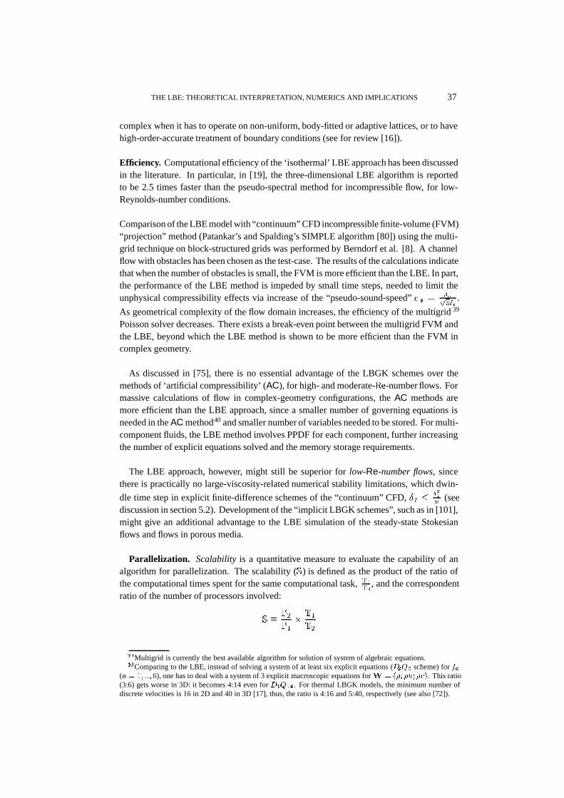
THE LBE: THEORETICAL INTERPRETATION, NUMERICS AND IMPLICATIONS 37
complex when it has to operate on non-uniform, body-fitted or adaptive lattices, or to havehigh-order-accurate treatment of boundary conditions (see for review [16]).
Efficiency. Computational efficiency of the ‘isothermal’ LBE approach has been discussedin the literature. In particular, in [19], the three-dimensional LBE algorithm is reportedto be 2.5 times faster than the pseudo-spectral method for incompressible flow, for low-Reynolds-number conditions.
Comparison of the LBE model with “continuum” CFD incompressible finite-volume (FVM)“projection” method (Patankar’s and Spalding’s SIMPLE algorithm [80]) using the multi-grid technique on block-structured grids was performed by Berndorf et al. [8]. A channelflow with obstacles has been chosen as the test-case. The results of the calculations indicatethat when the number of obstacles is small, the FVM is more efficient than the LBE. In part,the performance of the LBE method is impeded by small time steps, needed to limit theunphysical compressibility effects via increase of the “pseudo-sound-speed” � � � Æ��
��.
As geometrical complexity of the flow domain increases, the efficiency of the multigrid 39
Poisson solver decreases. There exists a break-even point between the multigrid FVM andthe LBE, beyond which the LBE method is shown to be more efficient than the FVM incomplex geometry.
As discussed in [75], there is no essential advantage of the LBGK schemes over themethods of ‘artificial compressibility’ (AC), for high- and moderate-��-number flows. Formassive calculations of flow in complex-geometry configurations, the AC methods aremore efficient than the LBE approach, since a smaller number of governing equations isneeded in the AC method40 and smaller number of variables needed to be stored. For multi-component fluids, the LBE method involves PPDF for each component, further increasingthe number of explicit equations solved and the memory storage requirements.
The LBE approach, however, might still be superior for low-Re-number flows, sincethere is practically no large-viscosity-related numerical stability limitations, which dwin-
dle time step in explicit finite-difference schemes of the “continuum” CFD, Æ � � Æ��� (see
discussion in section 5.2). Development of the “implicit LBGK schemes”, such as in [101],might give an additional advantage to the LBE simulation of the steady-state Stokesianflows and flows in porous media.
Parallelization. Scalability is a quantitative measure to evaluate the capability of analgorithm for parallelization. The scalability (�) is defined as the product of the ratio ofthe computational times spent for the same computational task, ��
��, and the correspondent
ratio of the number of processors involved:
�� ��
�� ��
��
��Multigrid is currently the best available algorithm for solution of system of algebraic equations.��Comparing to the LBE, instead of solving a system of at least six explicit equations (���� scheme) for ��
( � � ��� �), one has to deal with a system of 3 explicit macroscopic equations for � � ��� ��� ���. This ratio(3:6) gets worse in 3D: it becomes 4:14 even for �����. For thermal LBGK models, the minimum number ofdiscrete velocities is 16 in 2D and 40 in 3D [17], thus, the ratio is 4:16 and 5:40, respectively (see also [72]).

38 NOURGALIEV, DINH, THEOFANOUS, AND JOSEPH
where� is the number of processors involved in the calculation. In the “ultimate paralleliza-tion” case, � � �. Parallelization of the LBE algorithm can be achieved by dividing thecomputational domain into� subdomains, corresponding to� processors available; solvingfor each subdomain on separate processor; and communicating data between processorsusing MPI [74]. This parallelization strategy is employed in many modern CFD codes[73]. We analyzed the scalability of the LBE method [74] and the “continuum” CFD finite-difference code for compressible fluid dynamics [73], [75], and found the scalability of bothmethods in the range 0.7 - 0.95. The LBE method involves a more complex stencil,and, thus,the network for inter-processor communication is more sophisticated. In two dimensions,each processor, instead of four neighbors of the “continuum” CFD finite-difference code 41,the ��(� LBE code requires eight neighbors42. More sophisticated processor-network isrequired in three dimensions, fig.1b. Closely related to this is the amount of information tobe ‘exchanged’ at the end of each time step. In the case of the LBE’s “stream-and-collide”��(� scheme, symbolically, �� float variables are being sent/received, corresponding tothree “streamed” PPDFs, ��, and eight neighbor-processors. For the finite-difference code,�� variables must be sent/received, corresponding to three conserved variables � ��� 8�and [4 ‘neighbor-processors’ 3 layers of the finite-difference stencil 43]. Based on theabove consideration, one can see that the LBE approach is not an advantageous scheme.
In summary, the LBE method is a “pseudocompressible” solver of incompressibleflows. It shares the advantages, disadvantages and limitations of this class of the com-putational fluid dynamics methods. This includes the simplicity and explicitness of thealgorithm, which requires no solution of the Poisson equation; the restrictive simulationtime step in order to maintain the low-Mach-number limit (incompressible flow); and theartificial compressibility effects, ��� � ���� �� ��� �� �� �, originating from both thelinearized “pseudo-equation of state” /"�� � ��
� and the discretization errors. Similarlyto the “pseudocompressible” methods of the continuum-based CFD, the LBE approach isefficient in parallelization and suitable for massive computation of incompressible flows incomplex geometry configurations, such as flow in porous media, particulate and suspensionmultiphase flows.
7. CONCLUDING REMARKS
The Lattice Boltzmann Equation (LBE) method is an alternative numerical scheme fordescription of incompressible hydrodynamics. The LBE method has potential to serve as anefficient solver for incompressible low-Re-number flows in complex geometries, includingporous media, particulate/suspension multiphase flows.
Computationally, the LBE method belongs to a class of the pseudocompressible solversof the Navier-Stokes equations for incompressible flow. As such, the LBE method possessesthe advantages (simplicity of algorithm, no Poisson equation solver) and limitations (re-
��We utilize the high-order-accurate (WENO�, [53]) conservative finite-difference characteristics-based ap-proach ([73]; [28]; [75]).
��See the “stencil” of the ���� in fig.1a.��The ‘size’ of the stencil for WENO� scheme is 3 [53].

THE LBE: THEORETICAL INTERPRETATION, NUMERICS AND IMPLICATIONS 39
strictive time step, artificial compressibility) characteristic of pseudocompressible methods.
Beyond the incompressible homogeneous fluid, the LBE method permits implementa-tion of phenomenological terms and rules to mimic complex-fluid behaviors in a capacitysimilar to that of the continuum-based models of hydrodynamics. In this respect, the LBEmodels so far failed to provide a consistent framework for intermolecular interactions bymaking use of the discrete kinetic origin of the LBE method. Application of the LBEmethods to multiphase situations is additionally limited by the admissable range of fluidproperties (density ratio, surface tension and kinematic viscosity); time and length scales;and the inability to represent energy transport.
Acknowledgement. This work was supported in part by the National Aeronautics and Space Administration
under grant No. NAG3-2119, Lawrence Livermore National Laboratory Contract B502686, and by the U.S.
Nuclear Regulatory Commission under Cooperative Agreement No. NRC-04-98-051. The interest and therefore
collaboration of D.Joseph was limited to the part of this paper dealing with homogeneous (single-phase) flows.
This paper grew out of an informal memo by D.Joseph “General Remarks and Questions about the Lattice
Boltzmann Method”, in which various flaws in the presentation of the LBE method were highlighted. The work of
D. Joseph was supported by the NSF, Fluid, Particulate and Hydraulic Systems and by the Engineering Research
Program of the Office of Basic Energy Sciences at the DOE.
REFERENCES
1. Aidun, C.K., and Lu, Y., Lattice-Boltzmann Simulation of Solid Particles Suspended in Fluid, JournalStatistical Physics, 81, 49-61, 1995.
2. Aidun, C.K., Lu, Y., and Ding, E., Direct Analysis of Particulate Suspensions With Inertia Using the DiscreteBoltzmann Equation, J. Fluid mech., 373, 287-311, 1998.
3. Alexander, F.J., Chen, S., and Sterling, J.D., Lattice Boltzmann Thermohydrodynamics, Physical Review E,47 (4), R2249-R2252.
4. Andersen, D.M., McFadden, G.B., and Wheeler, A.A., Diffuse-Interface in Fluid Mechanics, Annual Reviewof Fluid Mechanics, 30, 139-165, 1998.
5. Aris, R., Vectors, Tensors, and the Basic Equations of Fluid Mechanics, Prentice-Hall, Inc., Englewood Cliffs,N.J., 1962.
6. Batchelor, G.K., An Introduction to Fluid Dynamics, Cambridge: Cambridge University Press, 1967.
7. Bhatnagar, P.L., Gross, E.P., and Krook, M., Model for Collision Processes in Gases, Phys. Rev., 94, 511,1954.
8. Bernsdorf, J., Durst, F., and Schafer, A., Comparison of Cellular Automata and Finite Volume Techniques forSimulation of Incompressible Flows in Complex Geometries, Int. J. for Numer. Meth. Fluids, 29, 251-264,1999.
9. Bobylev, A.V., The Chapman-Enskog and Grad methods for Solving the Boltzmann Equation, Sov. Phys.Dokl., 27, 1982.
10. Boghosian, B.M., and Coveney, P.V., Inverse Chapman-Enskog Derivation of the ThermohydrodynamicLattice-BGK Model for the Ideal Gas, International Journal of Modern Physics C, 9 (8), 1231-1245, 1998.
11. Bogoliubov, N.N., Problems of a Dynamical Theory in Statistical Physics, Moscow, 1946, ( English transl. in“Studies in Statistical Mechanics”, J.De Boer and G.E.Uhlenbeck, eds., Vol.I, North-Holland Publ., Amster-dam, 1962).
12. Boltzmann, L., Weitere Studien uber das Warmegleichgewicht unter Gasmoleculen, Wien Ber., 66, 275, 1872.Translation in English can be found in: Brush, S.G., Selected Readings in Physics, Kinetic Theory, Volume2. Irreversible Processes. Boltzmann, L., “Further Studies on the Thermal Equilibrium of Gas Molecules”,pp.88-175, 1966 Pergamon Press Ltd.
13. Cahn, J. W., and Hilliard, J. E., Free Energy of a Nonuniform System. 1. Interfacial Free Energy. J. Chem.Phys., 28(2), 258-267 (1958).

40 NOURGALIEV, DINH, THEOFANOUS, AND JOSEPH
14. Cercignani, C., Mathematical Methods in Kinetic Theory, Plenum Press, New York, 1969.
15. Chapmann, S., and Cowling, T.G., The Mathematical Theory of Non-Uniform Gases, Cambridge UniversityPress, 1970.
16. Chen, S., and Doolen, G. D., Lattice Boltzmann Method for Fluid Flows, Annu. Rev. Fluid Mech., 30 (4),329-364.
17. Chen, Y., Ohashi, H., and Akiyama, M., Thermal Lattice Bhatnagar-Gross-Krook Model Without NonlinearDeviations in Macrodynamic Equations, Physical Review E, 50 (4), 2776-2783.
18. Chen, Y., and Ohashi, H., Lattice-BGK Methods for Simulating Incompressible Fluid Flows, InternationalJournal of Modern Physics C, 8 (4), 793-803.
19. Chen, S., Wang, Z., Shan, X., and Doolen, G.D., Lattice Boltzmann Computational Fluid Dynamics in ThreeDimensions, Journal of Statistical Physics, 68 (3/4), 379-400.
20. Chorin, A.J., A Numerical Method for Solving Incompressible Viscous Flow Problems, Journal of Computa-tional Physics, 2, 12, 1967. Recent edition: 135, 118-125, 1997.
21. Cohen, E.G.D., Bogolubov and Kinetic Theory: The Bogolubov Equations, Mathematical Models & Methodsin Applied Sciences, 7(7) (1997), 909-933.
22. Dell’Isola, F., Gouin, H., and Seppecher, P., Radius and Surface Tension of Microscopic Bubbles be SecondGradient Theory, C. R. Acad. Sci. Paris, 320, 211-216.
23. Ding, E. and Aidun, C.K., The dynamics and scaling law for particles suspended in shear flow with inertia, J.Fluid Mech., 423, 317-344, 2000.
24. Drew, D.A., Passman, S.L., Theory of Multicomponent Fluids, Applied Mathematical Sciences 135, Springer,1999.
25. Eggels, J.G.M., Direct and Large-Eddy Simulation of Turbulent Fluid Flow using the Lattice-BoltzmannScheme, Int. J. Heat and Fluid Flow, 17 (1996), 307-323.
26. Eggels, J.G.M., and Somers, J.A., Numerical Simulation of Free Convective Flow using the Lattice-BoltzmannScheme, Int. J. Heat and Fluid Flow, 16 (1995), 357-364.
27. Enskog, D., Kungl. Svenska Vetenskaps Akademiens Handl., 63(4), 1921.
28. Fedkiw, R., Merriman, B., Donat, R., and Osher, S., The Penultimate Scheme for Systems of ConservationLaws: Finite Difference ENO with Marquina’s Flux Splitting, Progress in Numerical Solutions of PartialDifferential Equations, Arcachon, France, edited by M. Hafez, July 1998.
29. Felderhof, B.U., Dynamics of the diffuse gas-liquid interface near the critical point, Physica, 48 (1970),541-560.
30. Feng, J., Hu, H.H., and Joseph, D.D., Direct Simulation of Initial Value Problems for the Motion of SolidBodies in a Newtonian Fluid. Part 2. Couette and Poiseuille Flows, J. Fluid mech., 277, 271-301, 1994.
31. Frisch, U., Hasslacher, B., and Pomeau, Y., Lattice gas Cellular Automata for the Navier-Stokes equations,Phys. Rev. Lett., 56 (1986), 1505.
32. Gibbs, J.W., On the equilibrium of heterogeneous substances, Trans. Conn. Acad., 3:108-248, 3:343-524,1878. Reprinted in The Scientific Papers of J. Willard Gibbs, pp.55-371. London: Longmans, Green, and Co,1906.
33. Goldstein, S., Burgers, J.M., Lectures on Fluid Mechanics, Interscience Publishers, Ltd., London, 1957.
34. Gonnella, G., Orlandini, E., and Yeomans, J.M., Lattice-Boltzmann Simulation of Complex Fluids, Interna-tional Journal of Modern Physics, 8(4), 783-792.
35. Grad, H., On the Kinetic Theory of Rarified Gases, Communications on Pure and Applied Mathematics, 2(4),pp.331-407, 1949.
36. Guangwu, Y., Yaosong, C., and Shouxin, H., Simple Lattice Boltzmann Model for Simulating Flows withShock Wave, Physical Review E, January 1999, 59 (1), 454-459.
37. Gurtin, M.E., Polignone, D., and Vinals, J., Two-Phase Binary Fluids and Immiscible Fluids Described by anOrder Parameter, Mathematical Models and Methods in Applied Sciences, 6, 815 (1996).
38. Gustensen, A.K., Rothman, D.H., Zaleski, S., and Zanetti, G., Lattice Boltzmann Model of Immiscible Fluids,Phys. Rev. A., 43, 4320-4327 (1991).
39. Harris, S., An Introduction to the Theory of the Boltzmann Equation, Holt, Rinehart and Winston, New York,1971.
40. He, X., Chen,S., and Zhang, R., A Lattice Boltzmann Scheme for Incompressible Multiphase Flow and ItsApplication in Simulation of Rayleigh-Taylor Instability, Journal of Computational Physics, 152, 642-663(1999).

THE LBE: THEORETICAL INTERPRETATION, NUMERICS AND IMPLICATIONS 41
41. He, X., and Luo, L. -S., Lattice Boltzmann Model for the Incompressible Navier-Stokes Equation, Journal ofStatistical Physics, 88 (3/4), 1997, 927-944.
42. He, X., and Luo, L. -S., A priori Derivation of the Lattice Boltzmann Equation, Physical Review E, June1997, 55 (6), 6811-6817.
43. He, X., and Luo, L. -S., Theory of the Lattice Boltzmann: From the Boltzmann Equation to the LatticeBoltzmann Equation, Physical Review E, December 1997, 56 (6), 6811-6817.
44. He, X., Shan, X., and Doolen, G., Discrete Boltzmann equation model for nonideal gases, Physical ReviewLetters, January 1998, 57 (1), R13-R16.
45. He, X., Private communication.
46. Hirt, C.W., Nichols, B.D., Volume of Fluid (VOF) methods for the dynamics of free boundaries, Journal ofComputational Physics, 39, 201-225.
47. Hohenberg, B.I., and Halperin, P.C., Theory of Dynamic Critical Phenomena, Reviews of Modern Physics,49(3), 435-479 (1977).
48. Holdych, D.J., Rovas, D., Geogiadis, J.G., and Buckius, R.O., An improved Hydrodynamic Formulation forMultiphase Flow Lattice Boltzmann Models, International Journal of Modern Physics C, 9(8), 1393, (1998).
49. Huang, K., Statistical Mechanics, John Wiley & Sons, Inc., 1963.
50. Huang, J., Xu, F., Vallieres, H., Feng, D.H., Qian, Y.-H., Fryxell, B., and Strayer, M.R., A Thermal LBGKModel for Large Density and Temperature Differences, International Journal of Modern Physics C, 8 (4),827-841, 1997.
51. Ishii, M., Thermo-Fluid Dynamic Theory of Two-Phase Flow, Direction des Etudes et Recherches d’Electricitede France, 1975.
52. Jacqmin, D., An Energy Approach to the Continuum Surface Tension Method, AIAA 96-0858, In Pro-ceedings of the 34th Aerospace Sciences Meeting and Exhibit. Reno: American Institute of Aeronautics andAstronautics.
53. Jiang, G.S., and Shu, C.-W., Efficient Implementation of Weighted ENO Schemes, Journal of ComputationalPhysics, 126, 202-228, 1996.
54. Kirkwood, J.G., The Statistical Mechanical Theory of Transport Processes 2. Transport in Gases, J. of ChemicalPhysics, 15(1), pp.72-76, 1947.
55. Koga, T., Introduction to Kinetic Theory Stochastic Processes in Gaseous Systems, Pergamon Press, 1970.
56. Korteweg, D.J., Sur la forme que prennent les equations du mouvements des fluides si l’on tient compte desforces capillaires causees par des variations de densite considerables mais continues et sur la theorie de lacapillarite dans l’hypothese d’une variation continue de la densite, Arch. Neerl. Sci. Exactes Nat. Ser., II 6,1-24, 1901.
57. Klimontovich, Yu.L., Turbulent Motion and Chaos Structure: A New Approach to Statistical Theory of OpenSystems, Nauka, Moscow, (in Russian) 1990.
58. Ladd, A.J.C., Numerical Simulation of Particulate Suspensions via a Discretized Boltzmann Equation, Part 1.Theoretical Foundation, J. Fluid Mech., 271, 285-310, 1994.
59. Ladd, A.J.C., Numerical Simulation of Particulate Suspensions via a Discretized Boltzmann Equation, Part 2.Numerical Results, J. Fluid Mech., 271, 285-310, 1994.
60. Lallemand, P., and Luo, L.-S., Thery of the Lattice Boltzmann Method: Dispersion, Dissipation, Isotropy,Galilean Invariance, and Stablity, Physical Review E, June 2000, 61 (6), 6546-6562.
61. Lamb, H., "Hydrodynamics", Cambridge: Cambridge University Press, 1932.
62. Lamura, A., Gonnella, G., and Yeomans, J.M., A Lattice Boltzmann Model of Ternary Fluid Mixtures,Europhysics Letters, 1 February 1999, 99 (3), 314-320.
63. Landau, L. D., and Lifschitz, E. M., Theoretical Physics, v.VI, “Hydrodynamics”, Chapter II.15, In Russian,Nauka, Fourth Edition, 1988, Moscow.
64. Liboff, R.L., Introduction to the Theory of Kinetic Equations, John Wiley & Sons, Inc., 1969.
65. Luk’shin, A.V., Hydrodynamical Limit for the Boltzmann Equation and its Different Analogs, in NumericalMethods in Mathematical Physics, Moscow State University, Moscow (1986), 61-91.
66. Luo, L.- S., Unified Theory of Lattice Boltzmann Models for Nonideal Gases, Physical Review Letters, 24August 1998, 81 (8), 1618-1621.
67. Martys, N.S., and Chen, H., Simulation of Multicomponent Fluids in Complex Three-Dimensional Geometriesby the Lattice Boltzmann Method, Phys. Rev. E, 53, (1996), 743-750.

42 NOURGALIEV, DINH, THEOFANOUS, AND JOSEPH
68. Maxwell, J.C., Capillary Action. In Encyclopaedia Britannica, (9�� edition). Reprinted in The ScientificPapers of James Clerk Maxwell, 2, pp.541-591. New York: Dover, 1952.
69. McNamara, G.R. and Zanetti, G., Use of the Boltzmann Equation to Simulate Lattice-Gas Automata, Phys.Rev. Lett., 61, Number 20, (1988), 2332.
70. McNamara, G.R. and Alder, B., Analysis of the Lattice Boltzmann Treatment of Hydrodynamics, Physica A,194, (1993), 218-228.
71. McNamara, G.R., Garcia, A.L., and Alder, B.J., Stabilization of Thermal Lattice Boltzmann Models, Journalof Statistical Physics, 81, Number 1/2, (1995), 395-408.
72. McNamara, G.R., Garcia, A.L., and Alder, B.J., A Hydrodynamically Correct Thermal Lattice BoltzmannModel, Journal of Statistical Physics, 87, Number 5/6, (1997), 395-408.
73. Nourgaliev, R.R., Dinh, T.A., Dalal, D.C., Dinh, T.N., and Theofanous, T.G., MuSiC: Multiscale SimulationCode. “Modeling of Complex Fluid-Fluid and Fluid-Solid Interactions using the Level Set and ‘Ghost Fluid’Methodology. Single- and Multiphase Compressible Flows”, UCSB-CRSS Research Report, November 20,2000, 209p.
74. Nourgaliev, R.R., Dinh, T.N., and Sehgal, B.R., On Lattice Boltzmann Modeling of Phase Transitions in anIsothermal Non-Ideal Fluid, Nuclear Engineering and Design, 211, (2002), 153-171.
75. Nourgaliev, R.R., Dinh, T.N., and Theofanous, T.G., The ‘Numerical Acoustic Relaxation (NAR)’ Methodfor Time-Dependent Incompressible Single- and Multiphase Flows, CD-ROM Proceedings of The FourthInternational Conference on Multiphase Flows, May-June 2001, New Orlean, USA.
76. Oran, E. S., and Boris, J. P., Numerical Simulation of Reactive Flow, Elsevier Science Publishing Co., Inc.,New York-Amsterdam-London, 1987.
77. Qian, Y. H., D’Humieres, D., and Lallemand, P., Lattice BGK Models for Navier-Stokes Equation, EurophysicsLetters, 17 (6), 479-484.
78. Qian, Y. H., and Orszag, S.A., Lattice BGK Models for the Navier-Stokes Equation: Nonlinear Deviation inCompressible Regimes, Europhys. Lett., 21(3), 255-259, 1993.
79. Qian, Y. H., and Zhou, Y., Complete Galilean-Invariant Lattice BGK Models for the Navier-Stokes Equation,NASA/CR-1998-208701, ICASE Report No.98-38, August 1998.
80. Patankar, S.V., and Spalding, D.B., A Calculation Procedure for Heat, Mass and Momentum Transfer inThree-Dimensional Parabolic Flows, Int. J. Heat Mass Transf., 15, 1787-1806, 1972.
81. Poisson, S.D., Nouvelle Theorie de l’action capillaire, Paris: Bachelier, 1831.
82. Lord Rayleigh, On the theory of surface forces. - II. Compressible fluids. Phil. Mag., 33, pp.209-220, 1892.
83. Rider, W. J. , Approximate Projections Methods for Incompressible Flow: Implementation, Variants andRobustness, Technical Report LA-UR-2000, Los Alamos National Laboratory, 1994. Available on WorldWide Web at http://www.c3.lanl.gov/cic3/publications/main.html.
84. Rothman, D.H., and Zaleski, S., Lattice-Gas Cellular Automata: Simple models of complex hydrodynamics,Cambridge University Press, 1997.
85. Schulkes, R.M.S.M, The Evolution and Bifurcation of a Pendant Drop, J. Fluid Mech., 278, 83, 1994.
86. Sehgal, B.R., Nourgaliev, R.R., and Dinh, T.N., Numerical Simulation of Droplet Deformation and Break-Upby Lattice-Boltzmann Method, Progress in Nuclear Energy, 34(4), pp.471-488, 1999.
87. Seppecher, P., Moving Contact Lines in the Cahn-Hilliard Theory, Int. J. Engng. Sci, 34 (9), 977-992, 1996.
88. Sethian, J.A., Level Set Methods and Fast Marching Methods, Cambridge University Press, 1999.
89. Slemrod, M., Constitutive Relations for Monoatomic Gases Based on a Generalized Rational Approximationto the Sum of the Chapman-Enskog Expansion, Arch. Rational Mech. Anal., 150, 1-22, 1999.
90. Shan, X. and Chen, H., Lattice Boltzmann Model for Simulating Flows with Multiple Phases and Components,Physical Review E, March 1993, 47 (3), 1815-1819.
91. Shan, X. and Chen, H., Simulation of Nonideal Gases and Liquid-Gas Phase Transitions by the LatticeBoltzmann Equation, Physical Review E, April 1994, 49 (4), 2941-2948.
92. Shan, X. and Doolen, G., Multicomponent Lattice-Boltzmann Model with Interparticle Interactions, Journalof Statistical Physics, 81 (1/2), 379-393.
93. Shan, X. and Doolen, G., Diffusion in a Multicomponent Lattice Boltzmann Equation Model, PhysicalReview E, October 1996, 54 (4), 3614-3620.
94. Sterling, J.D., and Chen, S., Stability Analysis of Lattice Boltzmann Methods, Journal of ComputationalPhysics, 123, 196-206, 1996.
THE LBE: THEORETICAL INTERPRETATION, NUMERICS AND IMPLICATIONS 43
95. Sun, C., Adaptive Lattice Boltzmann Model for Compressible Flows: Viscous and Conductive Properties,Physical Review E, March 2000, 61 (3), 2645-2653.
96. Swift, M. R., Osborn, W. R. and Yeomans, J. M., Lattice Boltzmann Simulations of Nonideal Fluid, PhysicalReview E, November 1996, 54 (5), 5041-5052.
97. Swift, M. R., Orlandini, E., Osborn, W. R. and Yeomans, J. M., Lattice Boltzmann Simulations of Liquid-Gasand Binary Fluid Systems, Physical Review Letters, 31 July 1995, 75 (5), 830-833.
98. Teng, S. L., Chen, Y., and Ohashi, H., Lattice Boltzmann Simulation of Multiphase Fluid Flows through theTotal Variation Diminishing with Artificial Compression Scheme, Int. J. of Heat and Fluid Flow, 21, 112-121,2000.
99. Unverdi, S.O., Tryggvason, G., A Front-Tracking Method for Viscous, Incompressible, Multi-Fluid Flows,Journal of Computational Physics, 100, 25-37, 1992.
100. van der Waals, Verhandel. Konink. Akad. Weten. Amsterdam (Sect. 1), vol. 1, No. 8 (Dutch). Transl. J.S.Rowlinson, 1979, Translation of J.D. van der Waals’ "The thermodynamic theory of capillarity under thehypothesis of a continuous density variation", J. Stat. Phys., 20, 197-244.
101. Verberg, R., and Ladd, A.J.C., Simulation of Low-Reynolds-Number Flow via a Time-Independent Lattice-Boltzmann Method, Physical Review E, 60 (3), 3366-3373.
102. Wagner, A.J., and Yeomans, J.M., Effect of Shear on Droplets in a Binary Mixture, International Journal ofModern Physics C, 8 (4), 773-782.
103. Wolfram, S., Cellular Automation Fluids 1: Basic Theory, Journal of Statistical Physics, 45 (3/4), 471-526.
104. Yang, Z.L., Dinh, T.N., Nourgaliev, R.R., and Sehgal, B.R., Numerical Investigation of Bubble Growth andDetachment by the Lattice-Boltzmann Method, International Journal of Heat and Transfer, 44, pp.195-206,2001.
105. Zhang, D.F., Stone, H.A., Drop formation in viscous flows at a vertical capillary tube, Phys. Fluids, 9, 2234,1997.

44 NOURGALIEV, DINH, THEOFANOUS, AND JOSEPH
APPENDIX A
Lattice geometry and symmetry
Consider the lattice composed of � sublattices in � dimensions. Each sublattice hasweight )�, which is chosen to satisfy certain symmetry requirements. In total, the latticehas � � �� ��� � links, ��.
The most important properties of the lattice are related to the symmetries of the tensors:
�� � ���� � �
��
)������������ � ������� � (A.1)
which are determined from the choice of the basic lattice directions � �.The basic condition for standard hydrodynamic behaviour is that tensors � ��� for $ � �
should be isotropic [103]. Isotropic tensors � ��� , obtained with sets of � vectors ��
composing � sublattices in � space dimensions, must take the form�������� � �
����� � ���������� (A.2)
where %&&&&'&&&&(
���� �� � Æ �
���� ������ � Æ �Æ�� � Æ �Æ�� � Æ �Æ��
����� � ���� ��
�
�����
Æ � �������� ���� ��� ������ ��
(A.3)
Coefficients ����� in eq.(A.2) are dependent on the specific lattice geometry, and aregiven in Table 1 for the most commonly used lattices.
APPENDIX B
Equilibrium distribution function
In accordance to the Chapman-Enskog procedure (section 5.1), the equilibrium distribu-tion function should satisfy the following constraints:��
�� �eq� � ‘Mass conservation’��
�� �eq� ��� � � ‘Momentum conservation’
����
� eq� ������� �� �#� � �
� / �� � � �� ‘Momentum flux tensor’
����
� eq� ���������� �� ��� � � �
� ��� Æ�� � ��Æ � � ��Æ �� ‘Constitutive physics’
(B.1)
where � and / �� are the coefficient related to the fluid viscosity and pressure tensor,respectively.
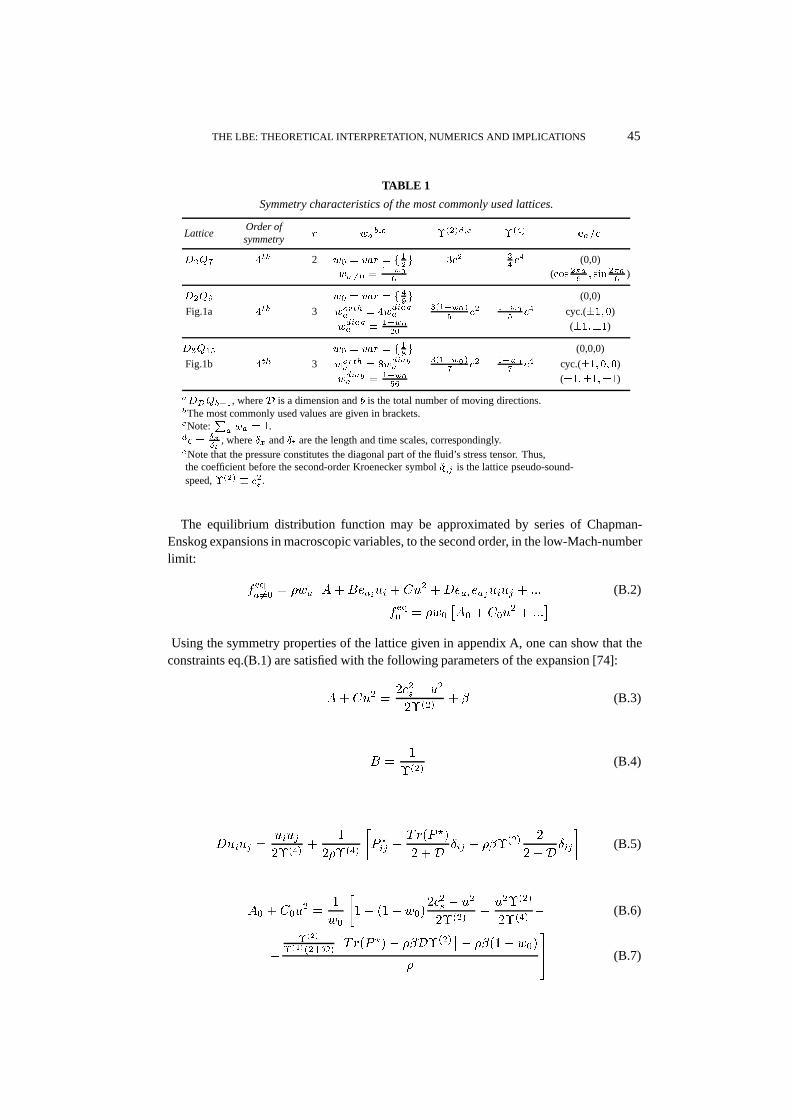
THE LBE: THEORETICAL INTERPRETATION, NUMERICS AND IMPLICATIONS 45
TABLE 1
Symmetry characteristics of the most commonly used lattices.
LatticeOrder ofsymmetry
� �� �� ������ ���
����
���� ��� 2 �� � �� � ��� ��� �
��� (0,0)
����� � �����
(��� ����
� ��� ����
)
���� �� � �� � ��� (0,0)
Fig.1a ��� 3 ������ � ������
�������
��� ����
��� cyc.(�� �)
������ � ����
��(���)
����� �� � �� � �� (0,0,0)
Fig.1b ��� 3 ������ � ������
�������
��� ����
��� cyc.(�� �� �)
������ � ����
��(�����)
���� ��, where � is a dimension and is the total number of moving directions. The most commonly used values are given in brackets.�Note:
�� �� � .
�� � ��
, where Æ� and Æ� are the length and time scales, correspondingly.�Note that the pressure constitutes the diagonal part of the fluid’s stress tensor. Thus,the coefficient before the second-order Kroenecker symbol Æ��� is the lattice pseudo-sound-speed, ��� � ��� .
The equilibrium distribution function may be approximated by series of Chapman-Enskog expansions in macroscopic variables, to the second order, in the low-Mach-numberlimit:
������ � )�
�������� � ��� ��������� �� � ���
�(B.2)
���� � )�
��� � ���
� � ����
Using the symmetry properties of the lattice given in appendix A, one can show that theconstraints eq.(B.1) are satisfied with the following parameters of the expansion [74]:
�� ��� ���� � ��
����� 9 (B.3)
� ��
����(B.4)
�� �� �� ������
��
����
/ � � �
���/ ��
�� Æ � � 9����
�� Æ �
(B.5)
�� � ���� �
�
)�
�� ��� )��
��� � ��
����� ������
����� (B.6)
����
�������
����/ ��� 9�����
�� 9��� )��
)* (B.7)

46 NOURGALIEV, DINH, THEOFANOUS, AND JOSEPH
where 9 is a free parameter, � is a space dimension, and ���/ �� is a trace of the nonidealpart of the pressure tensor, / �
�� � / �� � ���Æ �� .
Coefficient � is given by:
� � ����
����(B.8)
Setting 9 � � and / � �� � � (‘ideal fluid’), we can write � ��
� in the following compactform:
���� �
�� �� )�
������� �
��
�����
����� �� )�
����
�
��2����� � )�
���
����� ��
��������� ����
�������� ��
����
(B.9)
which are exactly the same equations as given in the LBE literature, [19] and [77]. Usingthe pressure tensor given by eq.(51) and the following equation for 9:
9 �/ �
� � 1 ��� ��
�� � �
�
�1 ��� �
�
���� (B.10)
where / �� � /� � ��
� is a ‘nonideal part’ of the equation of state, one can obtain the‘free-energy-based’ LBE model for ‘non-ideal fluid’ of Swift et al. [97].
In the ‘ideal fluid’ model, the lattice ‘pseudo-sound-speed’ is a function of the lattice sizeand time step, Æ� and Æ�, and the weight of the non-moving populations,) �, see Table 1. Inthe LBE literature, the value of )� is chosen in order to remove non-Navier-Stokes termsfrom the hydrodynamic equivalent of the LBE models. For the � �(� model, )� � �
� ,
[77]. In this case, the non-dimensional ‘pseudo-sound-speed’ is����
��� �
� .
APPENDIX C
Multiphase flow modeling
In this section, we provide a classification of the methods of computational fluid dy-namics (CFD) for multiphase, fluid-fluid flow. We will discuss only the ‘direct numericalsimulation’ (DNS) methods (i.e., those which resolve interface), putting aside ‘effectivefield’ methods, which employ statistically-/, time- or spatially-averaged equations for mul-tiphase systems ([24] [51]). The chief criterion used to classify a CFD method for DNS inmultiphase flow is the physical concept of interfaces.
1. “Free-Boundary Approach”, FBA . In this approach the interface between two im-miscible fluids is a free boundary which evolves in time. Equations of fluid motion holdin each fluid. These equations are supplemented by boundary conditions at the free sur-face, involving interfacial properties44. The formulation results in a free-boundary problem
��This approach originates from earliest works of Young, Laplace and Gauss, in 1800’s. They consideredthe interface between two fluids as a surface of zero thickness endowed with physical properties such as surfacetension.

THE LBE: THEORETICAL INTERPRETATION, NUMERICS AND IMPLICATIONS 47
(Lamb, 1932 [61], Batchelor, 1967 [6], etc.). Physical quantities, e.g. density and vis-cosity, are discontinuous across the interface. Physical processes such as e.g. capillarityoccurring at the interface, are represented by the boundary (“jump”) conditions imposedthere. Computational methods based on the “free-boundary” concept are the boundaryelement/boundary integral method, (BE/BIM) ([85] [105]).
2. “Physical-Diffuse-Interface Approach”, PDIA [4]. This approach is based on thePoisson’s (1831) [81] Maxwell’s (1876) [68] and Gibbs’s (1876) [32] concept of the inter-face as a rapid and smooth transition of physical properties between the bulk fluid values.The approach was further developed by Rayleigh (1892) [82] and van der Waals (1893)[100] with their “gradient theories for the interface” based on the thermodynamic princi-ples, and Korteweg (1901) [56], who proposed a constitutive law for the capillary stresstensor in terms of the density and its spatial gradients. Corresponding CFD methods arethe “second-gradient theory”, “phase-field” and “Model H” [47]. They all are based onthe “continuum mechanics methodology”, in which transport equations for macroscopicvariables are constructed, introducing the phenomenological physical models for interfacialdynamics through the effective forcing terms in the momentum equations (“capillary stresstensors”, “free-energy” concept, Cahn-Hilliard’s approach, etc.) and additional evolutionequations for “order” parameters. The “PDIA” CFD methods were used in a number ofapplications, including studies of critical point scaling laws [47], capillary waves [29],moving contact lines [87], droplets and nucleation [22], droplet breakup [52] and spinoidaldecomposition [37] (see for review [4]).
3. “Numerical-Diffuse-Interface Approach”, NDIA . The methods of this group in-volve a numerical scheme to “capture” or “track” the interface. The interface region isnumerically smeared-out over few computational nodes to allow a smooth transition offluid properties (i.e., density and viscosity). In this “numerical diffuse interface” region,the capillary effects are represented by “body forces” in the momentum equation, whichmimic the Korteweg’s capillary stress tensor. Advanced CFD developments in this classwere made with the “volume-of-fluid” method, VOF [46]; the level set equation method,LSA, [88]; and the “front-tracking” technique by Tryggvason [99].
APPENDIX D
Derivation of the viscous stress tensor for the LBGK models
In this section, we show the derivation of the viscous tensor for a LBGK model anddetailed formula for two other LBGK models. The non-Navier-Stokes terms are groupedinto an artifact tensor to enable a further assessment of the hydrodynamic equivalent of theLBE models.

48 NOURGALIEV, DINH, THEOFANOUS, AND JOSEPH
Isothermal ideal gas.
��� ���� �� � ��������
�� � ������
���� � � ����� � ��������� �� �
���� �
�� ������ �
���
�
������
���� � eq.(79) � ��
�����
���� � ������
���� � ��
������� � ����
����
���� �
� ����
� !������
����� �� ��$�
� ������� ��� �� �
���
� �����
����� ���� � ���
��� ��
�� �� �
�%� �� �Artifact
"###$
(D.1)
���� ���� and �
��� �� are given by eq.(B.1).
��� � ����
+,,,- ��
����
����� �� � ��� eq.(B.8)
�� Æ��� � ��Æ �� � ��Æ ���
)...* �
� ��
��� ���� � � ��� � ��� ���� � Æ ��
� �� �
�� �N.S. viscous stress tensor
� ��
�� �� ��� ��� ��� �� � �� ��� Æ ��
� �� �
�� �Artifact
(D.2)
Shear viscosity can be identified as
5 � �� � �� ��
���(D.3)
and
�� � ����
�� � � � /� � !�"# (D.4)
�$� � ����
�� ��
+,- ��
���� Æ ��� �� �����'����Æ� � � eq.(73)
� ��� � ��
).* �
� ����
�� ��
+,,,,,,-� �
������Æ ��� �� � �� �
� ������� Æ ��� �� � �� �
�� ��� ��� �� �eq.(74)
��� ��� � � �� �eq.(74)� �� �
�� �
)......*
(D.5)
Combining all terms, the viscous stress tensor is given by
��� ���� �� � ��
�5 ���� � � ��� �
�5 � 5��
����
��
����� � Æ ��
(D.6)
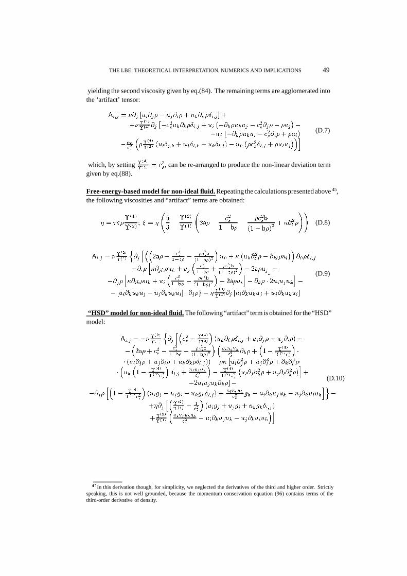
THE LBE: THEORETICAL INTERPRETATION, NUMERICS AND IMPLICATIONS 49
yielding the second viscosity given by eq.(84). The remaining terms are agglomerated intothe ‘artifact’ tensor:
� �� � ��� � �� � ��� � ���� Æ �� � �
�����
�� ����������� Æ �� � �
���� ���� � ����� � ��
��
������� ��� � ��
�� � � �
������
� ��
��� �� Æ��� � ��Æ �� � ��Æ ���� ��� ���Æ �� � � ��
�� (D.7)
which, by setting ��
��� � ���, can be re-arranged to produce the non-linear deviation term
given by eq.(88).
Free-energy-based model for non-ideal fluid.Repeating the calculations presented above 45,the following viscosities and “artifact” terms are obtained:
5 � �� ����
����� 6 � 5
��
��
����
����
�� � ��
�
�� � � ��
��
��� � �� � 1��
�
��(D.8)
� �� � ����
��
/��
���� � ���
���� ������
���������� � 1
����
�� � ��� ��
���� Æ ��
�� �1��� �� � ��
����
���� ������
��������� � ��
�
��� �1� � �� � �
����
���� ������
��������� � �
� �� � � ����
�
� � ������ � ������� � � �� � � 5���
�� �� � ������ � ������� �
(D.9)
“HSD” model for non-ideal fluid. The following “artifact” term is obtained for the “HSD”model:
� �� � �����
��
/��
����� � ��
���
������ Æ �� � � �� � ��� ��
��� � ��
� � ������� � �����
���������
���������
�� ���� ��
������
��
� �� �� � ��� � ���� Æ ����� 1�� �
�� � ���
� � ���
�� �
����
��� ��
������
�Æ �� �
���������
�� ��
������
�� ���
�� � ��� �
�� �
�
�� ������ �����
���� ��
������
��� 7� � ��7 � ��7�Æ ��� �
���������
7� � � ������ � ����� ��
0�
�5��
�����
�� � ����
��� 7� � ��7 � ��7�Æ ���
����
��
�������(�
���� � ������ � ����� ��
�
(D.10)
��In this derivation though, for simplicity, we neglected the derivatives of the third and higher order. Strictlyspeaking, this is not well grounded, because the momentum conservation equation (96) contains terms of thethird-order derivative of density.

50 NOURGALIEV, DINH, THEOFANOUS, AND JOSEPH
APPENDIX E
Evaluation of the deviations from the Navier-Stokes equations
IDEAL GAS MODELS
To estimate the order of the non-linear deviation term, we cast the LBGK hydrodynamicequation (89) into the following dimensional form:
�� � � �� �� � �� � Æ
��
� �� � ��� �� �� � �� � Æ
��
� � / � � ����� �
����
� �
� �� � ���� � � ����� �� �� �
����
�
��
� � ���� ���� ��� �� �
� �
�����
��
�� ����
�&�� � �
�����
��
����� ��
�(E.1)
where the Froude number is defined as � � ��
�
�� ; and � is an acceleration due to theexternal body force. The non-dimensional density variations are defined by eq.(93) and(94). It can be seen that the non-linear deviation term is negligibly small comparing to theNavier-Stokes equation terms under conditions46 ��� � � (or ���� � �, see Table 1).
In difference to our derivation, the LBGK hydrodynamic equations available in the liter-ature contain also linear deviations. For example, re-arranging the LBGK hydrodynamicequations given in [16] and [77] in a similar way as eq.(E.1), one can obtain the following“linear deviation term”:
�� ���� �� � �
��� � ���� � � ��� � � � ���� � � �
�� � ��� ��
�� �� �� �
��
�
��
� (E.2)
which is negligible in comparison to the Navier-Stokes terms in the limit Æ � � �.
The following linear and non-linear deviations can be obtained by re-arranging the LBGKhydrodynamic equations of ref. [78]:
�� ���� �� � ��� � ���� � � ��� �� �� �
� �
��
�
��
� ���� ���� �� � ������ � ����
���� �� �
� �
��
�
���� ��
� (E.3)
Both the linear and non-linear terms are negligible under conditions Æ � � � and ��� � �.
��Recently, Qian and Zhou [79] explored a way to eliminate the non-linear term by extending the “latticestencil” from 9 to 17 discrete velocities in 2D case.

THE LBE: THEORETICAL INTERPRETATION, NUMERICS AND IMPLICATIONS 51
Compressibility effects.It can be seen that the LBE model is not actually incompressiblein a “classical” fluid dynamics sense, which requires the velocity field be solenoidal��� �
� and � !�"#. There are always density variations and velocity divergence sourcespresent, due to the linearized “pseudo equation of state” / � � �
� (see eqs.(E.5) and(E.6)). The undesirable compressibility effects are minor as long as density variations
are small47�48, � � �Æ ��, � � �Æ
��, � �
��
�
��
�, and thermodynamic effects are not
considered.
Velocitydivergence sources ��������
� � ���
� ��� �� � �� �� � �Æ
��
����� �� � �� �� � �Æ
��
� � �%�� Æ � � Æ ���
� �� �Compressibility effects (Mass)
(E.5)
IncompressibleNavier-Stokes Part ��� ����
� � ���
� ����� � �� �� � ���
� �'�"� �� ����
� ��
���
� ��� � ���� � � ����� �� �� �
����
�
Deviationfrom
IncompressibleNavier-Stokes
Compressibility effects (Momentum)� �� ��� �� �� � �� �� � �Æ
��
�� �� �� � �� �
� � �%�� Æ �� Æ
���
�� ���� � � ��� � �� �� � �� �� �
��
�
��
�
Non-linear deviation: � �
�����
��
���� ��
�&�� � �
�����
��
���� �� �
�
� �� ���
��� ���� �� �
(E.6)
��Several LBGK models were developed in an attempt to reduce these compressibility effects [18] [41]. Inparticular, He and Luo [41] utilized the Chorin’s “pseudo-compressibility” method [20], in which instead ofeq.(63) the following macroscopic ‘pressure’ equation is introduced:
������ � ���� � � (E.4)
Instead of the mass and momentum, the � and �� are conserved. Eqs.(E.4) and (83) become a ‘target’macroscopic model for the “heuristical” building of the equilibrium distribution function. In the case of the steadyflow, this model completely recovers the ‘divergence-free’ velocity field. In the case of the transient flow, therequirement Æ�� � is still necessary to keep the divergence sources be suppressed.
�Another “incompressible” LBE model is due to Chen and Ohashi [18], in which the incompressibilitycondition �� is regained by applying the velocity correction - an idea borrowed from the ‘projection’ methods[83].

52 NOURGALIEV, DINH, THEOFANOUS, AND JOSEPH
FREE-ENERGY BASED MODELS
The “linear deviation tensor” of the free-energy-based model of the Swift et al. can bewritten in the following form:
�� ���� �� � �
���
%&&&&&&&&&&'&&&&&&&&&&(��
+,,,,,,,,,,-
� !
�� � ��
�
�� � � ��
��
��� � ��
���� �� �
� �
��
�
��
��1����
�� � ��� ��
�� �� �� �
��
�
��������
�
"##########$�� Æ �� �
��
+,,,,,,,,,,-
1��� ��� �� �� �
��
�
��������
� ���
����
�� � �
����
��� � ��
�� � ��� �� �
� �
��
�
��
�
)..........*� (E.7)
���
+,,,,,,,,,,-
1� � ��� �� �� �
��
�
��������
� ��
����
�� � �
����
��� � ��
�� � � � �� �
� �
��
�
��
�
)..........*
)..........*
1&&&&&&&&&&2&&&&&&&&&&3
and the “non-linear deviation tensor” is:
���� ���� �� � � /
����� � ������ � ������� ��
� �
��� �� �� � � ����� � � ������ � ������� � � �� �� �� �
� �
�����
��
������
� (E.8)
The linear deviation term includes the unphysical capillary terms of order� �
��
�
���� �� ��
�.
Comparison of these terms with the capillary stress tensor and the Navier-Stokes viscousstress tensor gives
�� ���� ��
� ��� �
��
���� �� � Æ
����
�

THE LBE: THEORETICAL INTERPRETATION, NUMERICS AND IMPLICATIONS 53
and
�� ���� ��
��� �� � �
�Æ
�
� � Æ �
�
������
�
which indicates that in order to have the unphysical surface tension suppressed, one has tokeep large ���.
Furthermore, the “linear deviation term” includes terms of unphysical viscous stresses
of the order � �
��
�
��
�. Comparison of these “artifacts” with the Navier-Stokes viscous
stress tensor:
�� ���� ��
��� �� � �
�Æ
�
� � Æ �
�
indicates that these unphysical terms cannot be neglected for large density differences ��
�, even for conditions of large ‘pseudo-sound-speed’, �� � � �. This is one of the
reasons why this LBGK scheme suffers from few unphysical effects, such as Galileaninvariance problem, [97] and section 4.7.2.
Non-linear deviation. Unphysical viscous stresses due to the non-linear deviation can besuppressed by keeping large ‘pseudo-sound-speed’, �� � � �,
���� ���� ��
� ��� �
�:�
����Æ �
�and
���� ���� ��
��� �� � �
��
����
�
HE-SHAN-DOOLEN MODEL
The “linear deviation” tensor is:
�� ���� �� � � �
���
����� 1 �� ��
� � ���� �
�� ���
�� � ��� �
�� ����
� �� �� �
��
�����
��
��������
� (E.9)
Comparing this unphysical term with capillary and viscous stress tensors:
������� �
�� �� �
�����
��
������
�������� �
'��� � � �
��
�
������
� (E.10)
indicates that keeping large ��� � �, this “artifact” can be considered as negligibly small,even for large density ratios
��
��� �, which is significant improvement in comparison to
the “free-energy-based” approach.
The “non-linear deviation” tensor is given by the following equation:

54 NOURGALIEV, DINH, THEOFANOUS, AND JOSEPH
���� ���� �� � � �
���
%&&&&&&&&&&'&&&&&&&&&&(��
+,,,,,,,,,,-��� � ��
� ����
�� � � ��
��
��� � ��
�� �������
�� � �� �� �
��
�
������
��
� 1
����
�� � � ����
���
� �� �� �
��
�����
��
�������
�� � ������ � �� �
� �
��
�
������
�
)...........*�
���
+,,,,,,,,,-
� �������
7�� �� �� �
��
�
�������
��� ������ � ����� ��� �� �
� �
��
�
������
�
).........*
1&&&&&&&&&2&&&&&&&&&3
�
(E.11)
� /�����
+,,,,,,,,,-
� ����7����� �� �
� �
��
�������
��� ������ � ����� ��� �� �
� �
��
������
�
).........*
and includes terms of order � �
����
����
�
�������
�and � �
����
�
������
�, which allows to
make this unphysical term be suppressed by keeping the limit �� � � �.