Abrupt and glacial-interglacial variability

Antonio García-Olivares ICM-CSIC

Barcelona, Spain agolivares@icm.csic.es

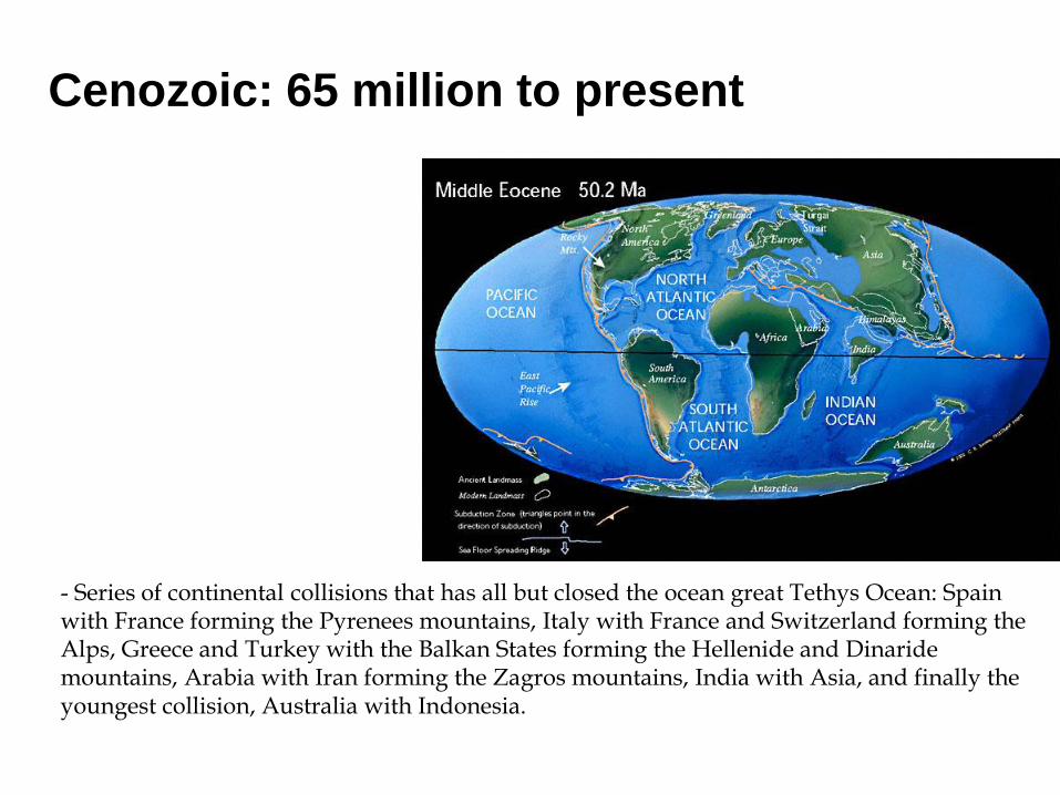
- Series of continental collisions that has all but closed the ocean great Tethys Ocean: Spain with France forming the Pyrenees mountains, Italy with France and Switzerland forming the Alps, Greece and Turkey with the Balkan States forming the Hellenide and Dinaride mountains, Arabia with Iran forming the Zagros mountains, India with Asia, and finally the youngest collision, Australia with Indonesia.

Cenozoic: 65 million to present

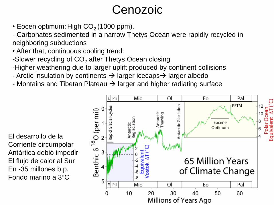
Cenozoic

• Eocen optimum: High CO2 (1000 ppm).

- Carbonates sedimented in a narrow Thetys Ocean were rapidly recycled in

neighboring subductions

• After that, continuous cooling trend:

-Slower recycling of CO2 after Thetys Ocean closing

-Higher weathering due to larger uplift produced by continent collisions

- Arctic insulation by continents larger icecaps larger albedo

- Montains and Tibetan Plateau larger and higher radiating surface

El desarrollo de la

Corriente circumpolar

Antártica debió impedir

El flujo de calor al Sur

En -35 millones b.p.

Fondo marino a 3ºC

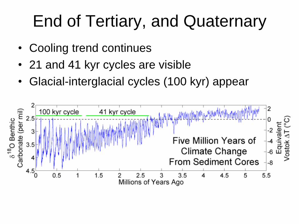
End of Tertiary, and Quaternary

• Cooling trend continues

• 21 and 41 kyr cycles are visible

• Glacial-interglacial cycles (100 kyr) appear

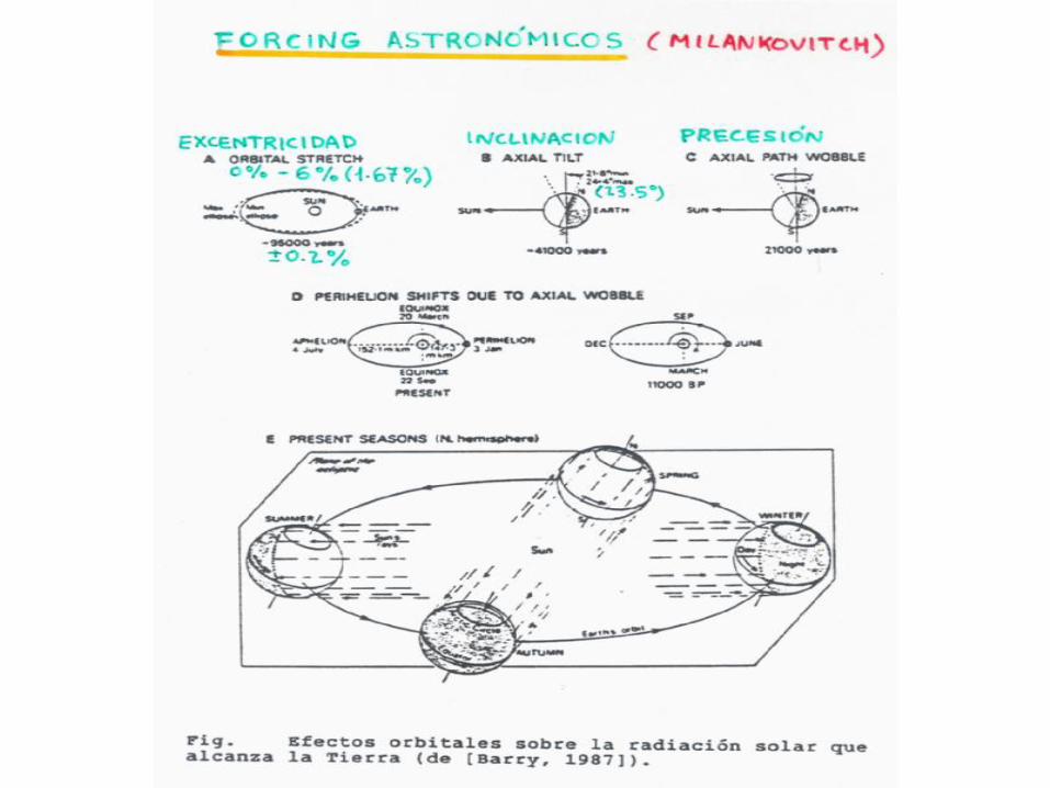
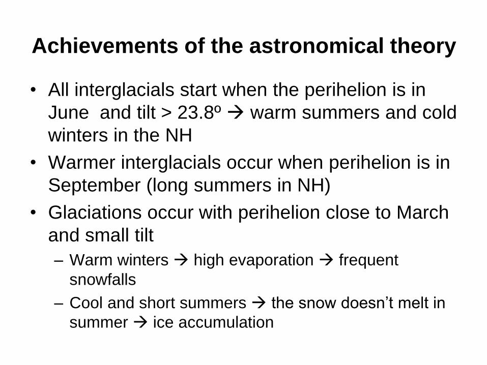
Achievements of the astronomical theory

• All interglacials start when the perihelion is in

June and tilt > 23.8º warm summers and cold

winters in the NH

• Warmer interglacials occur when perihelion is in

September (long summers in NH)

• Glaciations occur with perihelion close to March

and small tilt

– Warm winters high evaporation frequent

snowfalls

– Cool and short summers the snow doesn’t melt in

summer ice accumulation

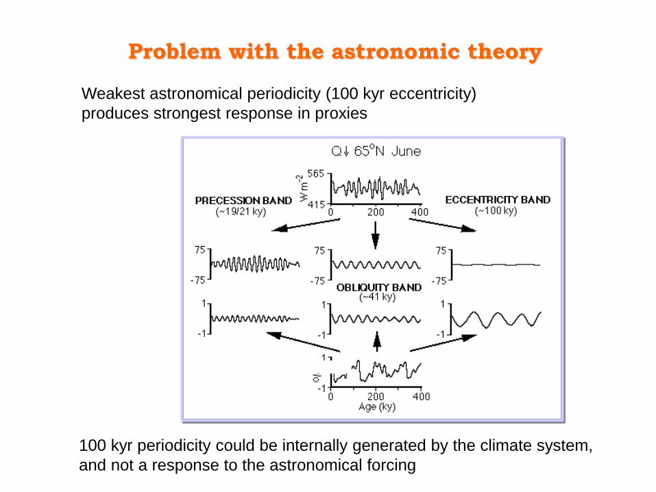
Problem with the astronomic theory

Weakest astronomical periodicity (100 kyr eccentricity)

produces strongest response in proxies

100 kyr periodicity could be internally generated by the climate system,

and not a response to the astronomical forcing

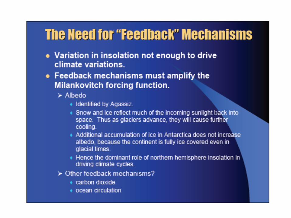
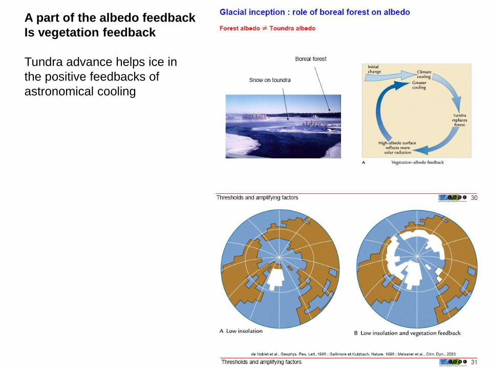
A part of the albedo feedback

Is vegetation feedback

Tundra advance helps ice in

the positive feedbacks of

astronomical cooling

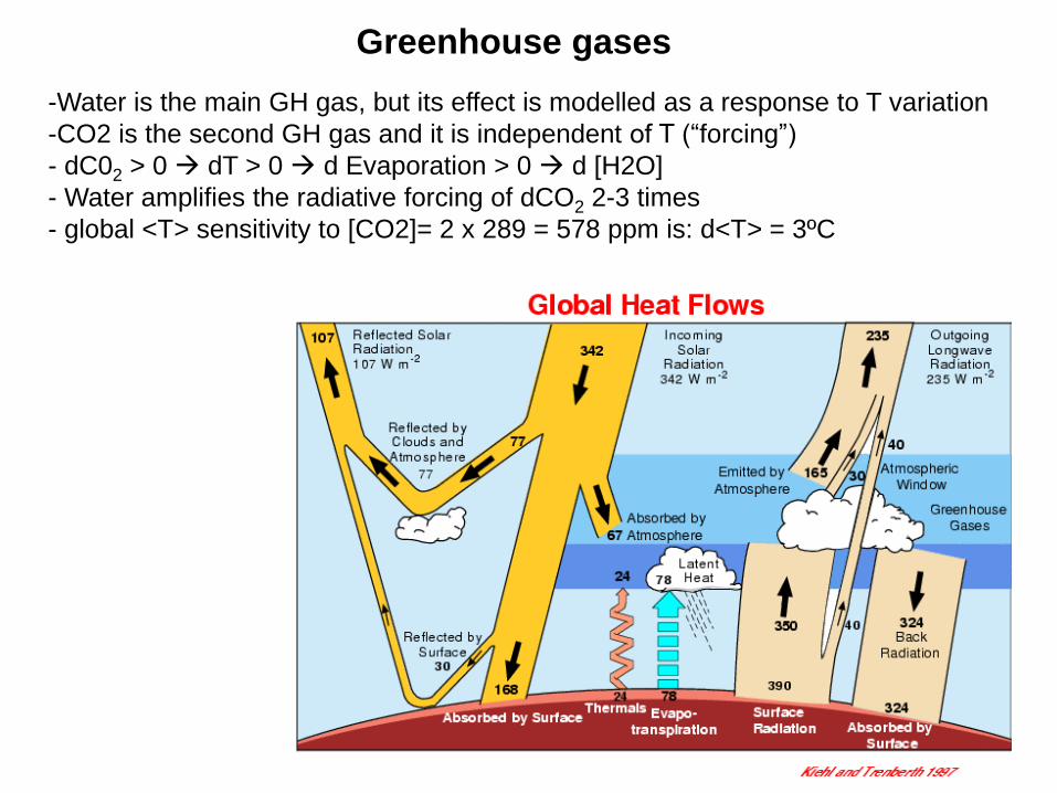
Greenhouse gases

-Water is the main GH gas, but its effect is modelled as a response to T variation

-CO2 is the second GH gas and it is independent of T (“forcing”)

- dC02 > 0 dT > 0 d Evaporation > 0 d [H2O]

- Water amplifies the radiative forcing of dCO2 2-3 times

- global <T> sensitivity to [CO2]= 2 x 289 = 578 ppm is: d<T> = 3ºC

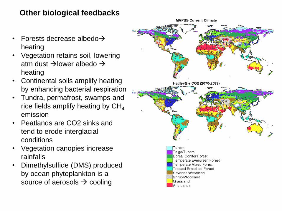
Other biological feedbacks

• Forests decrease albedo

heating

• Vegetation retains soil, lowering

atm dust lower albedo

heating

• Continental soils amplify heating

by enhancing bacterial respiration

• Tundra, permafrost, swamps and

rice fields amplify heating by CH4

emission

• Peatlands are CO2 sinks and

tend to erode interglacial

conditions

• Vegetation canopies increase

rainfalls

• Dimethylsulfide (DMS) produced

by ocean phytoplankton is a

source of aerosols cooling

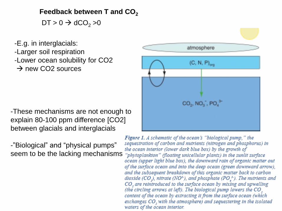
Feedback between T and CO2

DT > 0 dCO2 >0

-E.g. in interglacials:

-Larger soil respiration

-Lower ocean solubility for CO2

new CO2 sources

-These mechanisms are not enough to

explain 80-100 ppm difference [CO2]

between glacials and interglacials

-”Biological” and “physical pumps”

seem to be the lacking mechanisms

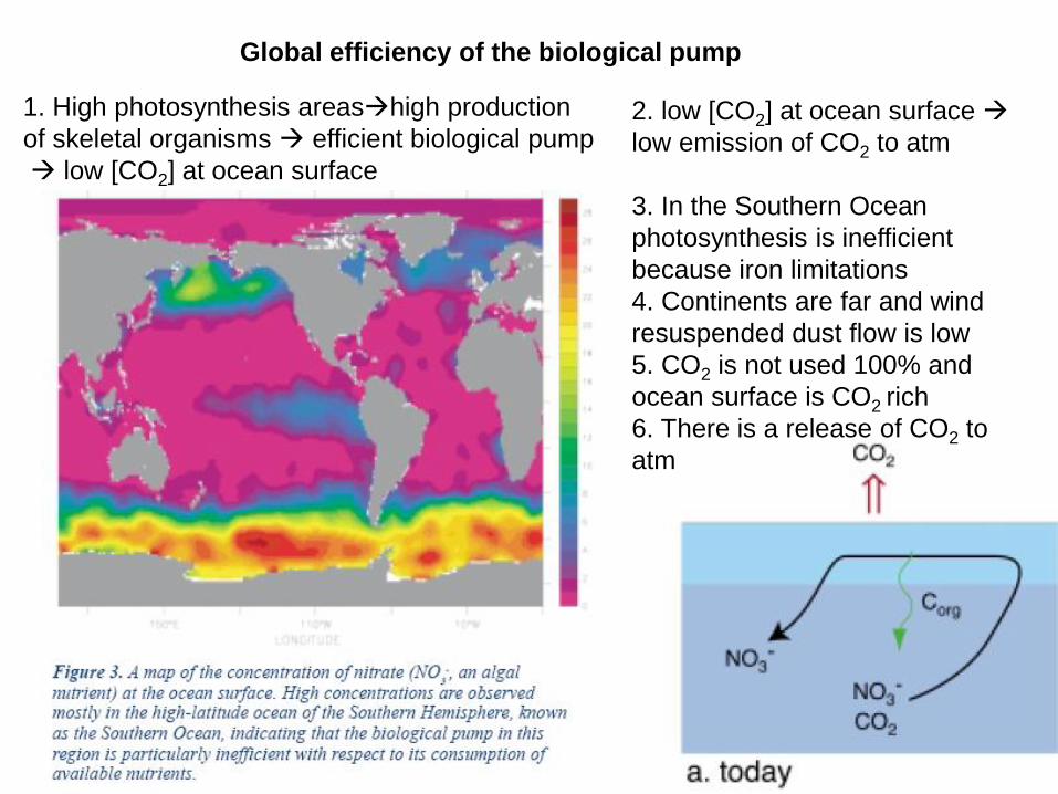
Global efficiency of the biological pump

2. low [CO2] at ocean surface

low emission of CO2 to atm

3. In the Southern Ocean

photosynthesis is inefficient

because iron limitations

4. Continents are far and wind

resuspended dust flow is low

5. CO2 is not used 100% and

ocean surface is CO2 rich

6. There is a release of CO2 to

atm

1. High photosynthesis areashigh production

of skeletal organisms efficient biological pump

low [CO2] at ocean surface

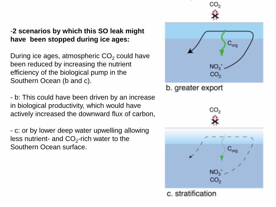
-2 scenarios by which this SO leak might

have been stopped during ice ages:

During ice ages, atmospheric CO2 could have

been reduced by increasing the nutrient

efficiency of the biological pump in the

Southern Ocean (b and c).

- b: This could have been driven by an increase

in biological productivity, which would have

actively increased the downward flux of carbon,

- c: or by lower deep water upwelling allowing

less nutrient- and CO2-rich water to the

Southern Ocean surface.

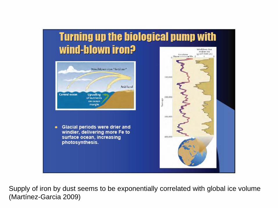
Supply of iron by dust seems to be exponentially correlated with global ice volume

(Martínez-Garcia 2009)

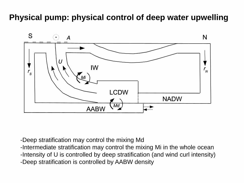
Physical pump: physical control of deep water upwelling

-Deep stratification may control the mixing Md

-Intermediate stratification may control the mixing Mi in the whole ocean

-Intensity of U is controlled by deep stratification (and wind curl intensity)

-Deep stratification is controlled by AABW density

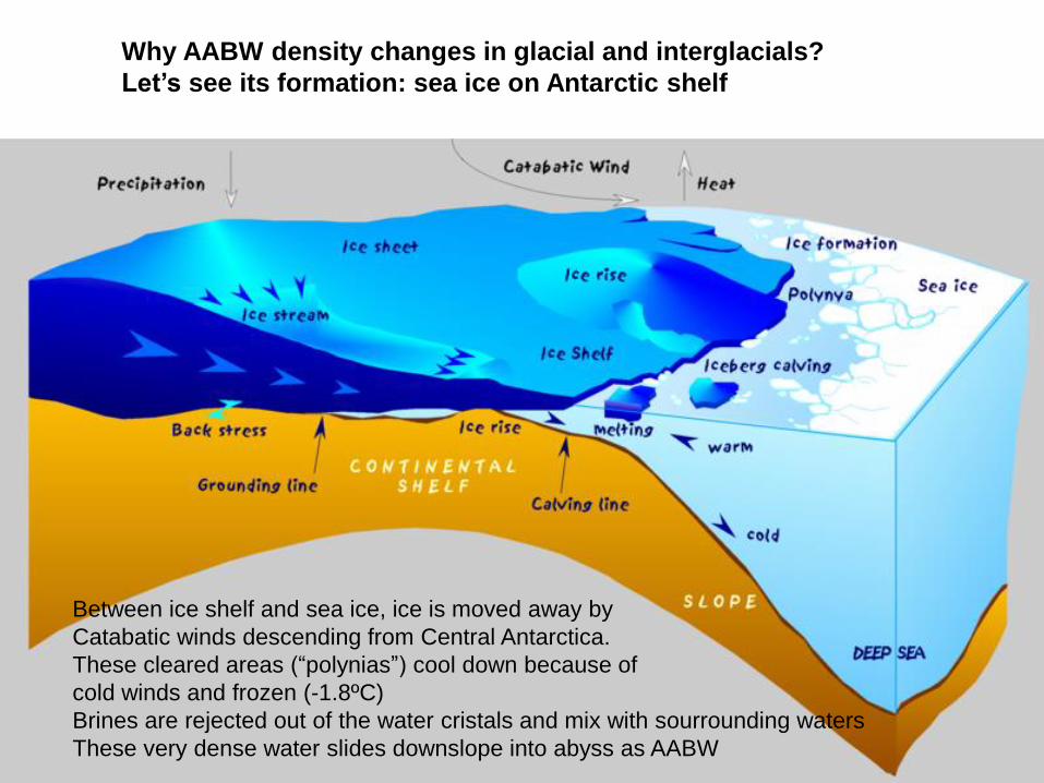
Why AABW density changes in glacial and interglacials?

Let’s see its formation: sea ice on Antarctic shelf

Between ice shelf and sea ice, ice is moved away by

Catabatic winds descending from Central Antarctica.

These cleared areas (“polynias”) cool down because of

cold winds and frozen (-1.8ºC)

Brines are rejected out of the water cristals and mix with sourrounding waters

These very dense water slides downslope into abyss as AABW

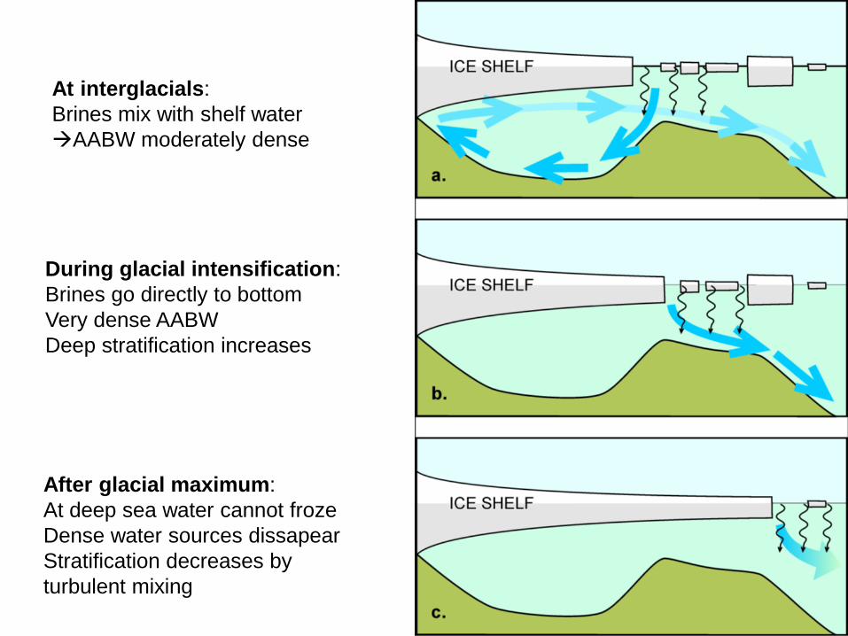
At interglacials:

Brines mix with shelf water

AABW moderately dense

During glacial intensification:

Brines go directly to bottom

Very dense AABW

Deep stratification increases

After glacial maximum:

At deep sea water cannot froze

Dense water sources dissapear

Stratification decreases by

turbulent mixing

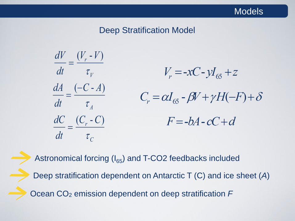
dV

dt(Vr -V )

V

dA

dt(C - A)

A

dC

dt(Cr -C)

C

Deep Stratification Model

Deep stratification dependent on Antarctic T (C) and ice sheet (A)

Ocean CO2 emission dependent on deep stratification F

Models

Astronomical forcing (I65) and T-CO2 feedbacks included

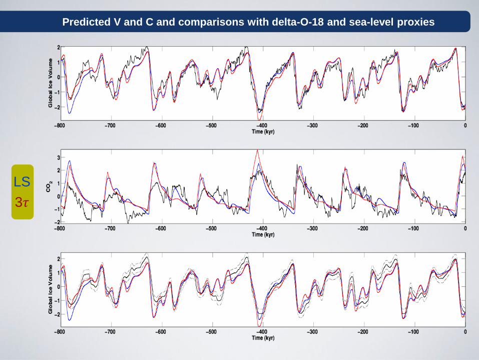
Predicted V and C and comparisons with delta-O-18 and sea-level proxies

3𝜏

LS

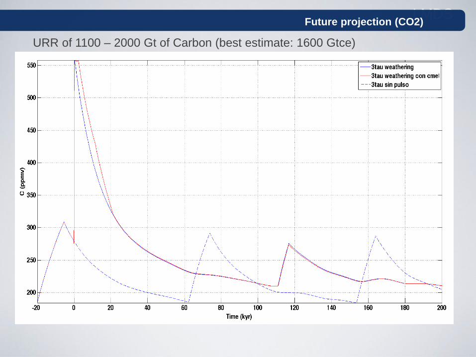
LMDS Future projection (CO2)

URR of 1100 – 2000 Gt of Carbon (best estimate: 1600 Gtce)

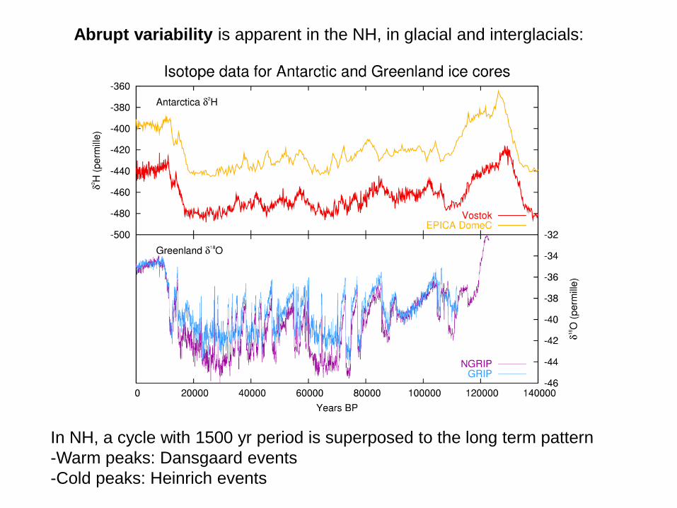
In NH, a cycle with 1500 yr period is superposed to the long term pattern

-Warm peaks: Dansgaard events

-Cold peaks: Heinrich events

Abrupt variability is apparent in the NH, in glacial and interglacials:

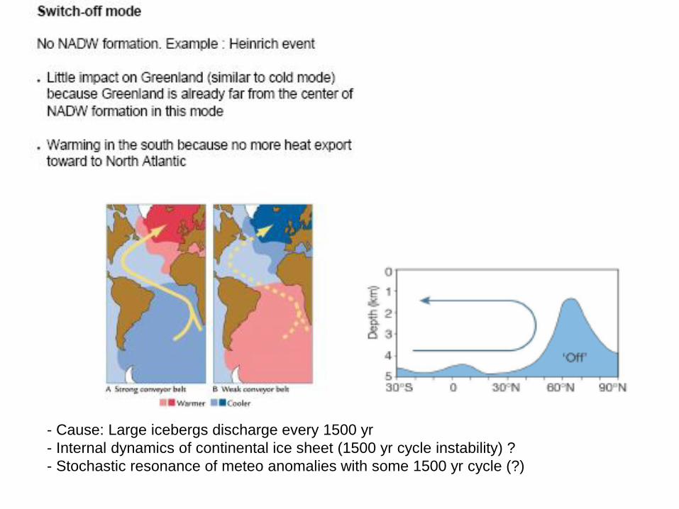
- Cause: Large icebergs discharge every 1500 yr

- Internal dynamics of continental ice sheet (1500 yr cycle instability) ?

- Stochastic resonance of meteo anomalies with some 1500 yr cycle (?)

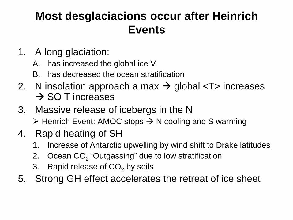
Most desglaciacions occur after Heinrich

Events

1. A long glaciation: A. has increased the global ice V

B. has decreased the ocean stratification

2. N insolation approach a max global <T> increases SO T increases

3. Massive release of icebergs in the N Henrich Event: AMOC stops N cooling and S warming

4. Rapid heating of SH 1. Increase of Antarctic upwelling by wind shift to Drake latitudes

2. Ocean CO2 “Outgassing” due to low stratification

3. Rapid release of CO2 by soils

5. Strong GH effect accelerates the retreat of ice sheet