Sea ice switch mechanism and glacial-interglacial CO ... · Sea ice switch mechanism and glacial-interglacial CO ... In this proposed mechanism the glacial oscillations ... start

Sea ice switch mechanism and glacial-interglacial CO2 variations

Hezi Gildor and Eli TzipermanEnvironmental Sciences, Weizmann Institute, Rehovot, Israel

J. R. ToggweilerGeophysical Fluid Dynamics Laboratory, Princeton, New Jersey, USA

Received 24 May 2001; revised 18 January 2002; accepted 23 January 2002; published 11 July 2002.

[1] A physical mechanism is proposed for the glacial-interglacial variations in the rate ofvertical mixing and in sea ice cover in the Southern Ocean. Such variations werepostulated without an explanation by Toggweiler [1999] and Stephens and Keeling[2000], who used them to explain the glacial-interglacial CO2 variations. In the physicalmechanism explored here, initially given by Gildor and Tziperman [2001b], changes inthe stratification of the Southern Ocean due to the cooling of North Atlantic Deep Water(NADW) during glacial maxima reduce the rate of vertical mixing of the surface waterwith the deep water. The changed temperature of the NADW arriving to the SouthernOcean and the reduced vertical mixing there also increase the Southern Ocean sea icecover during glacial maxima. These vertical mixing and sea ice cover changes are shownto be a natural result of the sea ice switch mechanism of the glacial cycles. A box model ofthe climate system is used to demonstrate the above physical mechanism and its effect onthe atmospheric CO2. Because of the uncertainties in the exact dependence of the verticalmixing on vertical stratification, it is impossible to quantify the exact separate contributionof reduced vertical mixing and larger sea ice cover to the glacial CO2 variations. The CO2

variations are not essential to the existence of the glacial cycles in the sea ice switchmechanism, yet they are shown to amplify the glacial-interglacial variability, consistentwith the view of the role of CO2 deduced from proxy observations. INDEX TERMS: 4806

Oceanography: Biological and Chemical: Carbon cycling; 4540 Oceanography: Physical: Ice mechanics and

air/sea/ice exchange processes; 3344 Meteorology and Atmospheric Dynamics: Paleoclimatology

1. Introduction

[2] The atmospheric concentration of CO2 has undergonesignificant and fairly regular variations on a timescale of100 kyr during at least the last four glacial-interglacialcycles [Petit et al., 1999], with concentrations duringglacial periods being �80 ppm less than during warmerinterglacial periods. Despite the effort invested in order toidentify the mechanism responsible for these variations inlight of the possible role it may play in global warming, agenerally accepted explanation is still missing [Pedersenand Bertrand, 2000; Sigman and Boyle, 2000]. Previousexplanations of this CO2 variability in terms of SouthernOcean productivity and vertical mixing changes [Wenk andSiegenthaler, 1985; Sarmiento and Toggweiler, 1984; Volkand Hoffert, 1985] ran into contradicting evidence fromvarious proxy indicators [Toggweiler, 1999]. The searchfor a mechanism, though, still seems focused on theSouthern Ocean as the key region [Pedersen and Bertrand,2000], although not exclusively [e.g., Daskal Hausmanand McElroy, 1999]. Stephens and Keeling [2000] sug-gested that an extended sea ice cover during glacial

periods reduced air-sea CO2 gas exchange. The extendedsea ice cover was specified in their model based onavailable proxy records, but they didn’t suggest a mech-anism that can explain the extended sea ice cover. Fran-cois et al. [1997] found evidence in the proxy record foran increased stratification southward of the polar front,which may have reduced the CO2 leak from the ocean toatmosphere. Similarly, Toggweiler [1999] used a biochem-ical box model to suggest that by considering the SouthernOcean to be an upwelling region rather than a downwel-ling region, as done in previous works, a change in thevertical mixing in the Southern Ocean can induce theobserved atmospheric CO2 changes and still remain con-sistent with available proxy observations. Toggweiler[1999], again, did not propose a physical mechanism fora reduced vertical mixing in the Southern Ocean duringglacial times.[3] Stephens and Keeling [2000] and Toggweiler [1999]

presented restricted glacial and interglacial steady statesolutions to their biochemical box models but could notexplain the transition between these states. Dealing with thetransition mechanism and explaining the changes in verticalmixing and sea ice cover clearly requires a physical mech-anism and model of the glacial-interglacial cycle that issufficiently detailed.

GLOBAL BIOGEOCHEMICAL CYCLES, VOL. 16, NO. 3, 10.1029/2001GB001446, 2002

Copyright 2002 by the American Geophysical Union.0886-6236/02/2001GB001446$12.00

6 - 1

[4] Such a physical mechanism and model for the 100-kyrglacial oscillations was presented by Gildor and Tziperman[2000, 2001a, 2001b], including simplified yet explicitmodel components for the oceanic meridional circulation,sea ice, land glaciers, and atmosphere. This ‘‘sea iceswitch’’ mechanism is based on a rapid switch-like growthand melting of the Northern Hemisphere sea ice. The seaice, in turn, shifts the land ice between growing and with-drawing modes, creating the observed sawtooth structureand 100-kyr timescale. Gildor and Tziperman [2001b] haveadded an ocean biochemistry model to the physical climatemodel of Gildor and Tziperman [2000, 2001a] and havepresented a detailed mechanism for the vertical mixing andsea ice changes arbitrarily specified by Toggweiler [1999]and Stephens and Keeling [2000]. The result is a possiblescenario for the glacial oscillations, including the reductionof atmospheric CO2 concentration during glacial periods,and the physical and biogeochemical mechanisms involvedin both the glacial and interglacial stages, as well as thetransitions between them.[5] The mechanism suggested by Gildor and Tziperman

[2001b] for the missing physics in the biochemical scenariosof Toggweiler [1999] and Stephens and Keeling [2000] maybe summarized as follows. During the present interglacialperiod the stratification in the Southern Ocean is composedof cold fresh upper water above salty and warmer NorthAtlantic Deep Water (NADW) arriving to the SouthernOcean from the north. Note that this deeper water mass isrelatively warm, also, due to mixing with surface midlatitudewater on its way from the North Atlantic. We propose thatduring the buildup stage of Northern Hemisphere ice sheetsthe deep water formed in the North Atlantic becomes colder.Similarly, the mixing with cooler glacial period surface waterin midlatitudes results in the subsurface deeper water arriv-ing colder and denser to the Southern Ocean. This is inagreement with proxy records that indicate colder deep waterin the Atlantic Ocean during the Last Glacial Maximum(LGM) [Schrag et al., 1996] and with model results thatshow that NADW formation continues somewhat reducedduring the LGM [Ganopolski et al., 1998; Weaver et al.,1998; Yu et al., 1996; Matsumoto and Lynch-Stieglitz, 1999]and that the outflow to the Southern Ocean then becomescolder [Weaver et al., 1998]. Because of the large ice massover Antarctica, the surface water in the Southern Ocean isalready very close to the freezing point, even during inter-glacial times, and cannot cool further during glacial maxima.The cooling of the deep water arriving from the NorthAtlantic therefore makes the stratification in the SouthernOcean more stable during glacial maxima, consistent withthe proxy records of Francois et al. [1997]. On the basis ofsimple arguments linking the stratification to vertical mixingby internal waves [Gargett, 1984], such a more stablestratification is expected to reduce the mixing between theCO2-rich deep water and the surface water [Sikes et al.,2000]. This results in the observed reduction in atmosphericCO2 during glacial periods, according to the mechanism ofToggweiler [1999]. The temperature, the vertical mixing,and the amount of the upwelling water also play key roles incontrolling the Southern Ocean’s sea ice [Gordon, 1981]:The reduced vertical mixing and the lower deep water

temperature result in a larger sea ice extension during coldperiods [Crosta et al., 1998]. This, in turn, can again reduceatmospheric CO2 according to the mechanism of Stephensand Keeling [2000], who specified the sea ice change with-out providing a mechanism.[6] In this proposed mechanism the glacial oscillations

exist due to a self-sustained internal variability of thephysical climate system, with Milankovitch forcing provid-ing the phase locking of the 100-kyr variability [Gildor andTziperman, 2000]. The CO2 changes are therefore not thedriving force of the glacial-interglacial oscillation [Loutreand Berger, 2000] but rather are induced by the physicalchanges to the Southern Ocean stratification and verticalmixing. These CO2 changes, in turn, also affect the atmos-pheric radiation, and amplify the physical signal of theglacial oscillations to some degree, consistent with othermodel results [Weaver et al., 1998] and with the recentinterpretation of the Vostok record [Petit et al., 1999].[7] In the present paper we extend the work of Gildor

and Tziperman [2001b], having in mind several specificobjectives. First, we try to separate the contribution ofchanges in the rate of vertical mixing and in the sea icecover to the glacial-interglacial CO2 variations. Second, inlight of the debate that arose recently in the literatureregarding the differences between box models and generalcirculation model (GCM) simulations of the carbon cycle[Archer et al., 2000b, 2000a; Broecker et al., 1999], we try totest the sensitivity of the proposed mechanism to variousprocesses that may contribute to these differences. (Thisissue is investigated more fully by J. Toggweiler et al.(Representation of the carbon cycle in box models andGCMs, 1, The solubility pump, and Representation of thecarbon cycle in box models and GCMs, 2, The organiccarbon pump, submitted to Global Biogeochemical Cycles,hereinafter referred to as T01a and T01b (available at http://www.ldeo.columbia.edu/�hezi/misc.html)) who demonstra-ted that with respect to organically cycled CO2, box modelsmay actually do a better job in simulating the partitioning ofCO2 between the ocean and the atmosphere.) Finally, wedescribe here the models used at a level of detail not possiblein the short format of Gildor and Tziperman [2001b]. Westart with a brief description of the physical model and itsvariation from a similar one used by Gildor and Tziperman[2000, 2001a] (section 2.1), describe the added biochemistrymodel (section 2.2), and explain the sea ice switch mecha-nism of glacial oscillations (section 3). Next, we combine thesea ice switch mechanism with the ocean biochemistrymodel and obtain the glacial atmospheric CO2 variabilitybased on the mechanism of Toggweiler [1999] (section 3.2).The sensitivity to the insulating effect of sea ice cover on theair-sea CO2 flux [Stephens and Keeling, 2000], to thevertical mixing, to the piston velocity, and to the deephorizontal mixing are examined in sections 4.1, 4.2, 4.3,and 4.4, respectively. We conclude in section 5.

2. Model Description

2.1. Submodels for Physical Climate Component

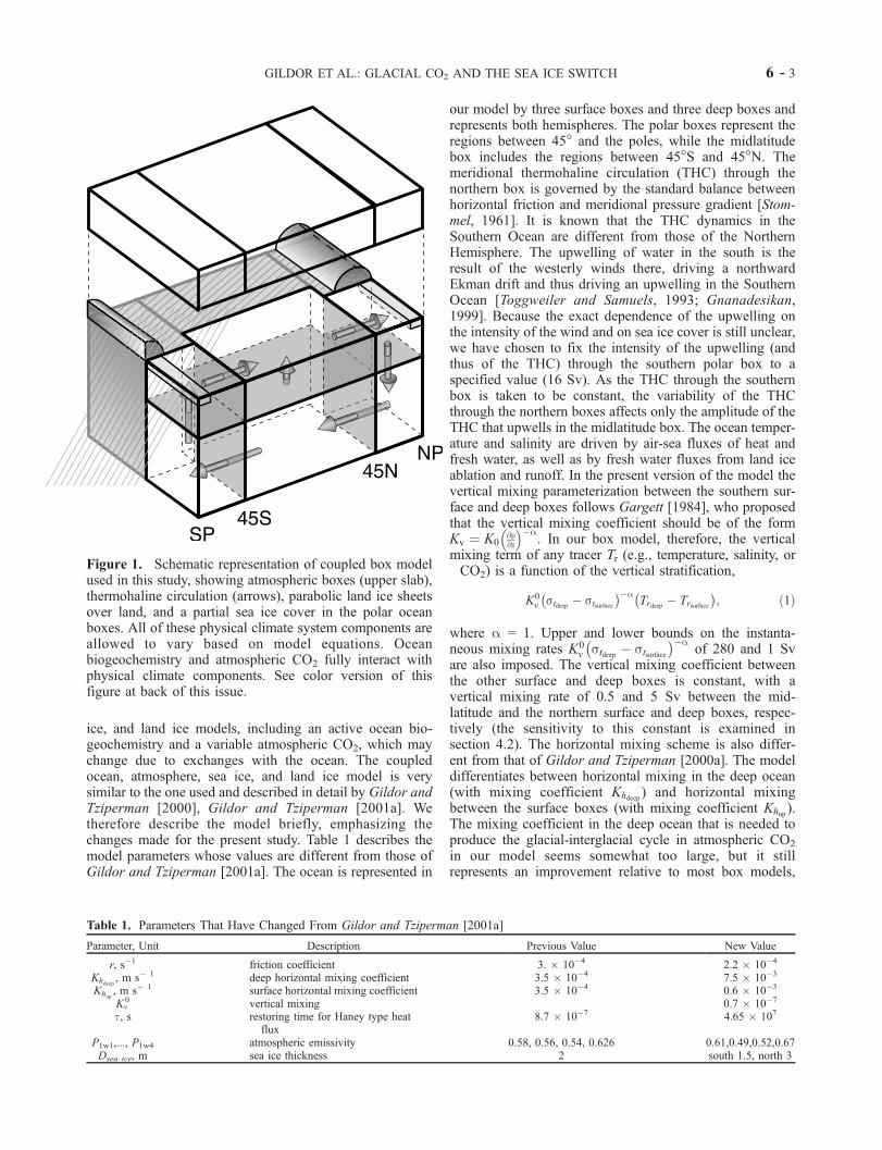
[8] Our coupled meridional box model, schematicallyshown in Figure 1, is composed of ocean, atmosphere, sea

6 - 2 GILDOR ET AL.: GLACIAL CO2 AND THE SEA ICE SWITCH

ice, and land ice models, including an active ocean bio-geochemistry and a variable atmospheric CO2, which maychange due to exchanges with the ocean. The coupledocean, atmosphere, sea ice, and land ice model is verysimilar to the one used and described in detail by Gildor andTziperman [2000], Gildor and Tziperman [2001a]. Wetherefore describe the model briefly, emphasizing thechanges made for the present study. Table 1 describes themodel parameters whose values are different from those ofGildor and Tziperman [2001a]. The ocean is represented in

our model by three surface boxes and three deep boxes andrepresents both hemispheres. The polar boxes represent theregions between 45� and the poles, while the midlatitudebox includes the regions between 45�S and 45�N. Themeridional thermohaline circulation (THC) through thenorthern box is governed by the standard balance betweenhorizontal friction and meridional pressure gradient [Stom-mel, 1961]. It is known that the THC dynamics in theSouthern Ocean are different from those of the NorthernHemisphere. The upwelling of water in the south is theresult of the westerly winds there, driving a northwardEkman drift and thus driving an upwelling in the SouthernOcean [Toggweiler and Samuels, 1993; Gnanadesikan,1999]. Because the exact dependence of the upwelling onthe intensity of the wind and on sea ice cover is still unclear,we have chosen to fix the intensity of the upwelling (andthus of the THC) through the southern polar box to aspecified value (16 Sv). As the THC through the southernbox is taken to be constant, the variability of the THCthrough the northern boxes affects only the amplitude of theTHC that upwells in the midlatitude box. The ocean temper-ature and salinity are driven by air-sea fluxes of heat andfresh water, as well as by fresh water fluxes from land iceablation and runoff. In the present version of the model thevertical mixing parameterization between the southern sur-face and deep boxes follows Gargett [1984], who proposedthat the vertical mixing coefficient should be of the formKv ¼ K0

@r@z

� ��a. In our box model, therefore, the vertical

mixing term of any tracer Tr (e.g., temperature, salinity, or�CO2) is a function of the vertical stratification,

K0v stdeep � stsurface� ��a

Trdeep � Trsurface� �

; ð1Þ

where a = 1. Upper and lower bounds on the instanta-neous mixing rates K0

v stdeep � stsurface� ��a

of 280 and 1 Svare also imposed. The vertical mixing coefficient betweenthe other surface and deep boxes is constant, with avertical mixing rate of 0.5 and 5 Sv between the mid-latitude and the northern surface and deep boxes, respec-tively (the sensitivity to this constant is examined insection 4.2). The horizontal mixing scheme is also differ-ent from that of Gildor and Tziperman [2000a]. The modeldifferentiates between horizontal mixing in the deep ocean(with mixing coefficient Khdeep ) and horizontal mixingbetween the surface boxes (with mixing coefficient Khup ).The mixing coefficient in the deep ocean that is needed toproduce the glacial-interglacial cycle in atmospheric CO2

in our model seems somewhat too large, but it stillrepresents an improvement relative to most box models,

Figure 1. Schematic representation of coupled box modelused in this study, showing atmospheric boxes (upper slab),thermohaline circulation (arrows), parabolic land ice sheetsover land, and a partial sea ice cover in the polar oceanboxes. All of these physical climate system components areallowed to vary based on model equations. Oceanbiogeochemistry and atmospheric CO2 fully interact withphysical climate components. See color version of thisfigure at back of this issue.

Table 1. Parameters That Have Changed From Gildor and Tziperman [2001a]

Parameter, Unit Description Previous Value New Value

r, s�1 friction coefficient 3. � 10�4 2.2 � 10�4

Khdeep, m s� 1 deep horizontal mixing coefficient 3.5 � 10�4 7.5 � 10�3

Khup, m s� 1 surface horizontal mixing coefficient 3.5 � 10�4 0.6 � 10�3

Kv0 vertical mixing 0.7 � 10�7

t, s restoring time for Haney type heatflux

8.7 � 10�7 4.65 � 107

P1w1,..., P1w4 atmospheric emissivity 0.58, 0.56, 0.54, 0.626 0.61,0.49,0.52,0.67Dsea ice, m sea ice thickness 2 south 1.5, north 3

GILDOR ET AL.: GLACIAL CO2 AND THE SEA ICE SWITCH 6 - 3

which treat the whole deep ocean as a single-value box[Toggweiler, 1999; Stephens and Keeling, 2000; Volk andHoffert, 1985; Wenk and Siegenthaler, 1985; Daskal Haus-man and McElroy, 1999].[9] Sea ice forms in our model when the ocean water

temperature decreases below a critical freezing temperatureand melts above that temperature. Following the observedcharacteristic of sea ice in both hemispheres, the sea icecover is assumed to grow in area within the northern andsouthern polar ocean boxes with an initial thickness of 3 and1.5 m, respectively, and then to become thicker if the entirepolar box is sea ice covered; sea ice presence and evolutionaffect the surface albedo, the salinity budget in the ocean,the air-sea heat flux, the CO2 flux, and evaporation bypartially insulating the ocean from the atmosphere. Theequation of state is the full nonlinear equation recommen-ded by U.N. Educational, Scientific, and Cultural Organ-ization [1981].[10] The atmospheric model is also similar to that used by

Gildor and Tziperman [2001a], with a few changes. In orderto improve the seasonality of sea ice cover, mainly in oursouthern box, we incorporate the important contribution ofshort-wave radiation to sea ice thermodynamics. The short-wave radiation term that influences the energy balance ofsea ice can be written as [Maykut and Perovich, 1987]

1� að Þ 1� i0ð ÞHin;

where a is the sea ice albedo and i0 is the fraction of the netshort-wave radiation that affects the atmospheric headbalance and does not contribute directly to surface melting.Although both a and i0 in reality are highly dependent onvariables such as the type of sea ice, its age, etc., here wetake them to be constants with the values of 0.65 and 0.57,respectively, giving together (1 � a)(1 � i0) = 0.15, i.e,15%. The present model uses 15% of the incoming short-wave radiation, Hin, for melting of sea ice if and where itexists. The rest of the short-wave radiation directlyinfluences the atmospheric heat balance, as before.[11] The lower surface of each atmospheric box is a

combination of ocean, land, land ice, and sea ice, each withits specified albedo. The averaged potential temperature ofeach atmospheric box is calculated based on the energybalance of the box.[12] The outgoing long-wave radiation in the ith box is

Hout = Plwi sq4, where s is the Stefan-Boltzmann constant

and Plwi is an emissivity coefficient that, in principal,

depends on cloud cover, aerosol, etc. and is thereforeallowed to vary here from box to box. In the present study,unlike in the work by Gildor and Tziperman [2000, 2001a],atmospheric CO2 is a prognostic variable that directly

affects the long-wave emissivity,

P ilw ¼ P i

lw;0 � K logCO2

COref2

; ð2Þ

where Plwi ,0 is taken to be constant in time, CO2 is the

atmospheric concentration of carbon dioxide, CO2ref is a

reference concentration taken to be 200 ppm, and K ischosen such that doubling the CO2 concentration will causea radiative forcing of 4 W m�2 [Ramanathan et al., 1987].[13] The model for northern land ice sheets, whose slow

evolution provides the 100-kyr timescale in our model, iszonally symmetric, assumes perfect plasticity [Weertman,1976; Ghil, 1994], grows due to the precipitation in thepolar boxes, and decreases due to ablation, ice runoff, andcalving processes.

2.2. Ocean Biogeochemistry Model

[14] Our biochemistry model is similar to those used inthree-dimensional (3-D) biochemical general circulationmodels [e.g., Bacastow and Maier-Reimer, 1990; Yama-naka, 1996]. Its parameters appear in Table 2. The modelincludes total CO2 (�CO2) and alkalinity (AT) (including thecomponents of the aqueous carbon and borate only) asprognostic variables that are used to calculate pCO2. PO4

is taken to be the limiting nutrient in our model, as iscommonly done in other model studies. This enables us todisregard the complex interaction between different compo-nents of the nitrogen cycle [Maier-Reimer, 1993]. Themodel is of the ‘‘closed-system’’ type [Sigman and Boyle,2000], so total alkalinity and PO4 are constant during theintegration, although their distribution in the ocean canchange. We also take into account the salinity and temper-ature calculated in the ocean model for calculation of thedissociation coefficients. Surface pCO2 is calculated basedon the �CO2, alkalinity, salinity, and temperature and iscomputed according to Yamanaka [1996].[15] The equations for �CO2, AT, and PO4 are similar to

those for the temperature and salinity, except for an addedsource/sink term Sp for the biochemistry variables,

Pt þ vPð Þyþ wPð Þz¼ KhPy þ KvPz þ Sp: ð3Þ

The source/sink is different for each variable, and theprocesses included in it are discussed below. Redfield ratiois the ratio between P:N:C (assumed constant 1:16:122) inparticulate organic matter. We denote the ratio P:N as RN

and denote the ratio P:C as RC. The rate of exportproduction, EP (the part of organic matter that is producedat the surface boxes and that sinks as particulate organicflux), depends on the latitude (via the light factor), the

Table 2. Biochemistry Model Parameters

Parameter, Unit Description Value

r1, r2, r3, mW productivity coefficient 6 � 10�7, 5. � 10�4, 1. � 10�4

PV, m s�1 piston velocity 5. � 10�5

TC0 initial averaged total CO2 2240, mmol, Kg�1

TA0 initial averaged total alkalinity 2371, mequiv, Kg�1

P0 initial averaged phosphate 2.09, mmol, Kg�1


amount of nutrients (PO4 in our model), and the ocean areanot covered by sea ice, Aopenwater, and is given by

EP ¼ rLf PO4½ Aopenwater; ð4Þ

where Lf is the light factor taken to be the averaged solarradiation at each box and [PO4] is the phosphateconcentration; r serves as a tuning parameter, which enablesus to take implicitly into account other factors that mayaffect the production, such as a lack of iron, and is thereforedifferent for each box. A more realistic parameterization(similar to Maier-Reimer [1993]) is

EP ¼ rLf PO4½ PO4½ hþ PO4½ ;

where h is a half-saturation constant and gives very similarresults in our model because the relatively large thickness ofthe upper boxes in our model ‘‘smoothes’’ the variations insurface concentration found in GCMs that resolve thethermocline with a few levels. The sinking particles fromeach surface box are assumed to be remineralized in thedeep box below. The specified ‘‘rain ratio’’ dictates the ratioof organic to inorganic carbon atoms extracted from the�CO2 pool per PO4 molecule that sinks as particulate flux.We use the same expression for the rain ratio (RR) as usedby Maier-Reimer [1993]

RR ¼ 61 exp 0:1 T � 10ð Þ½ = 1þ exp 0:1 T � 10ð Þ½ f g;

where T is the surface temperature. This expression gives anupper limit of 0.5 for the rain ratio.[16] The source/sink terms for �CO2, AT (total alkalinity),

and PO4 are affected by numerous processes. We nowconsider the processes included in the source/sink term foreach variable.2.2.1. �CO2

[17] Export production of organic soft tissue and of calciteshells reduces the �CO2 at the surface at rates of RC � EPand RR � EP, respectively, and remineralization increases�CO2 in the deep boxes at the same rates. Gas exchange ofCO2 between the atmosphere and the ocean also affects the�CO2 content of the ocean. The flux between the ocean andthe atmosphere is linear in the pCO2 difference between theatmosphere and the surface boxes of the ocean.

FCO2¼ PV CO2;a

� �� CO2;o

� �� Aopenwater; ð5Þ

where [CO2,a] is the saturation concentration with regard tothe partial pressure of CO2 in the atmosphere, [CO2,o] is theconcentration of CO2 in the ocean, and Aopenwater is theocean area not covered by sea ice, thus taking into accountthe influence of sea ice cover on the air-sea flux; PV is thepiston velocity [Siegenthaler and Sarmiento, 1993]. Addingall these terms, we find, for a given surface box,

SSCO2¼ �RC � EP� RR� EPþ PV CO2;a

� �� CO2;o

� ��

and for the deep box below it,

SSCO2¼ RC � EPþ RR� EP:

2.2.2. AT (Total Alkalinity)[18] The production of calcite shells at the surface reduces

the alkalinity there at a rate of 2 � RR � EP, and thedissolution of shells in the deep ocean increases the alka-linity at the same rate. The export production of soft tissueincreases the alkalinity at the surface boxes at a rate of RN �EP, and remineralization in the deep boxes decreases it,again at the same rate. The source term for a surface boxbecomes

SAT¼ �2� RR� EPþ RN � EP;

while for a deep box, the signs of the terms are opposite.2.2.3. PO4

[19] Export production from the surface and reminerali-zation in the deep ocean act as sink and source, respectively,for phosphate, at a rate of EP. Thus SPO4

¼ �EP at thesurface and has the opposite sign in the box below.

3. Results

[20] All runs analyzed in this paper are summarized inTable3. We begin by analyzing a physics-only model run(PHYSICS-ONLY) (Table 3) without the biochemistry oceanmodel and with a fixed atmospheric CO2 (section 3.1).Having briefly discussed the sea ice switch mechanism ofthe glacial oscillations using this simplified run, we thenadd the ocean biochemistry model, which induces atmos-pheric CO2 variability and therefore affects the atmos-pheric radiation balance (experiment BIO) (section 3.2).Then, sensitivity experiments are discussed in section 4. Inorder to test the effect of sea ice on the air-sea CO2 flux[Francois et al., 1997; Stephens and Keeling, 2000], werun experiment sea-ice-flux (SIF) (section 4.1), in whichthe existence of sea ice does not prevent CO2 flux between

Table 3. Experiments Summary

Experiment Code Description Figures

PHYSICS-ONLY no ocean biochemistry effects, only physicalcomponents of the climate system

2

BIO including ocean biochemistry 3SIF sea ice does not affect air-sea CO2 flux 6

VM_M oceanic vertical mixing in the midlatitude 7VM_S1, VM_S2 oceanic vertical mixing in the south with and

without insulating effect of sea ice8

PV1,PV2 changes in the piston velocity 9DM deep horizontal mixing 10


the ocean and the atmosphere, as it does in the full modeland in the actual climate system. The influence of thevertical mixing between the midlatitude surface and deepboxes is investigated in experiment VM_M, and thesensitivity to a different vertical mixing parameterizationbetween the surface and deep southern boxes is inves-tigated in run VM_S (section 4.2). In runs PV1 and PV2we check the sensitivity of the results to the pistonvelocity of air-sea CO2 exchange (section 4.3). Finally,we investigate the sensitivity to the rate of deep horizontalmixing (experiment DM) (section 4.4).

3.1. Physics-Only Run

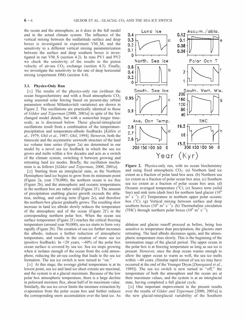
[21] The results of the physics-only run (without theocean biogeochemistry and with a fixed atmospheric CO2

using seasonal solar forcing based on present-day orbitalparameters without Milankovitch variations) are shown inFigure 2. The oscillations are practically identical to thoseof Gildor and Tziperman [2000, 2001a] in spite of the fewchanged model details, but with a somewhat longer time-scale, as is discussed below. These glacial-interglacialoscillations result from a combination of the temperature-precipitation and temperature-albedo feedbacks [Kallen etal., 1979; Ghil et al., 1987; Ghil, 1994]. However, both thetimescale and the asymmetric sawtooth structure of the landice volume time series (Figure 2a) are determined in ourmodel by a novel sea ice feedback in which the sea icegrows and melts within a few decades and acts as a switchof the climate system, switching it between growing andretreating land ice modes. Briefly, the oscillation mecha-nism is as follows [Gildor and Tziperman, 2000, 2001a].[22] Starting from an interglacial state, as the Northern

Hemisphere land ice begins to grow from its minimum point(Figure 2a, year 170,000), the northern ocean is ice free(Figure 2b), and the atmospheric and oceanic temperaturesin the northern box are rather mild (Figure 2f ). The amountof precipitation enabling glacier growth exceeds the abla-tion, melting, and calving term (Figure 2e), and thereforethe northern box glacier gradually grows. The resulting slowincrease in land ice albedo slowly reduces the temperatureof the atmosphere and of the ocean (Figure 2f ) in thecorresponding northern polar box. When the ocean seasurface temperature (Figure 2f ) reaches the critical freezingtemperature (around year 50,000), sea ice starts to form veryrapidly (Figure 2b). The creation of sea ice further increasesthe albedo, induces a further reduction of atmospherictemperature, and results in the creation of more sea ice(positive feedback). In <20 years, �60% of the polar boxocean surface is covered by sea ice. Sea ice stops growingwhen it isolates enough of the ocean from the cold atmos-phere, reducing the air-sea cooling that leads to the sea iceformation. The sea ice switch is now turned to ‘‘on.’’[23] At this stage, the average global temperature is at its

lowest point, sea ice and land ice sheet extents are maximal,and the system is at a glacial maximum. Because of the lowpolar box atmospheric temperature, there is a large declinein poleward moisture flux, about half of its maximum value.Similarly, the sea ice cover limits the moisture extraction byevaporation from the polar ocean box and further reducesthe corresponding snow accumulation over the land ice. As

ablation and glacier runoff proceed as before, being lesssensitive to temperature than precipitation, the glaciers startretreating. The land albedo decreases again, and the atmos-pheric temperature rises slowly. This is the beginning of thetermination stage of the glacial period. The upper ocean inthe polar box is at freezing temperature as long as sea ice ispresent. However, once the deep ocean warms enough toallow the upper ocean to warm as well, the sea ice meltswithin �40 years. (Similar rapid retreat of sea ice may haveoccurred at the end of the Younger Dryas [Dansgaard et al.,1989]). The sea ice switch is now turned to ‘‘off,’’ thetemperature of both the atmosphere and the ocean are attheir maximum values, and the system is at an interglacialstate, having completed a full glacial cycle.[24] One important improvement in the present results

over the results of Gildor and Tziperman [2000, 2001a] isthe new glacial-interglacial variability of the Southern

Figure 2. Physics-only run, with no ocean biochemistryand using fixed atmospheric CO2. (a) Northern land iceextent as a fraction of polar land box area. (b) Northern seaice extent as a fraction of polar ocean box area. (c) Southernsea ice extent as a fraction of polar ocean box area. (d)Oceanic averaged temperature (�C). (e) Source term (solidline) and sink term (dash line) for northern land glacier (106

m3 s�1). (f ) Temperature in northern upper polar oceanicbox (�C). (g) Vertical mixing between surface and deepsouthern boxes (106 m3 s�1). (h) Thermohaline circulation(THC) through northern polar boxes (106 m3 s�1).


Ocean and of the Southern Ocean sea ice cover, resultingfrom the improved parameterizations described in section 2.1(Figure 2c). While Southern Ocean sea ice exists throughoutthe model glacial cycle, its meridional extension now variesbetween glacial and interglacial states, as well as varyingwith the seasonal cycle, and depends on the conditions in theNorthern Hemisphere. When sea ice is present in ourmodel’s northern polar box, the deep water that is formedthere and that fills the deep ocean becomes colder. Thiscauses two effects that contribute to the increased extensionof southern sea ice: (1) The temperature of the upwellingwater in the Southern Ocean is colder, and (2) the verticalstratification in the Southern Ocean becomes more stable;hence less vertical mixing occurs between the surface anddeep southern polar boxes. The significant effect of theupwelling water on the evolution of sea ice in the SouthernOcean is known from both observational and model studies[Martinson, 1990; Gordon, 1981; Gordon and Huber,1990]. The reduced vertical mixing will be further discussedin section 3.2 and section 4.2 and will be seen later to playan important role in the glacial-interglacial CO2 cycle, whenthe biogeochemistry is activated, as expected from work byToggweiler [1999]. In turn, it will be shown that the CO2

cycle intensifies the glacial-interglacial cycle of the South-ern Ocean sea ice extent. Unlike in the work by Toggweiler[1999], the vertical mixing and the THC in our model arenot specified, but are calculated by the model equations andvary during the glacial-interglacial cycles. Consistent withobservations, the THC through our northern box weakensduring cold glacial periods [Boyle and Keigwin, 1987].

3.2. Biogeochemistry Effects

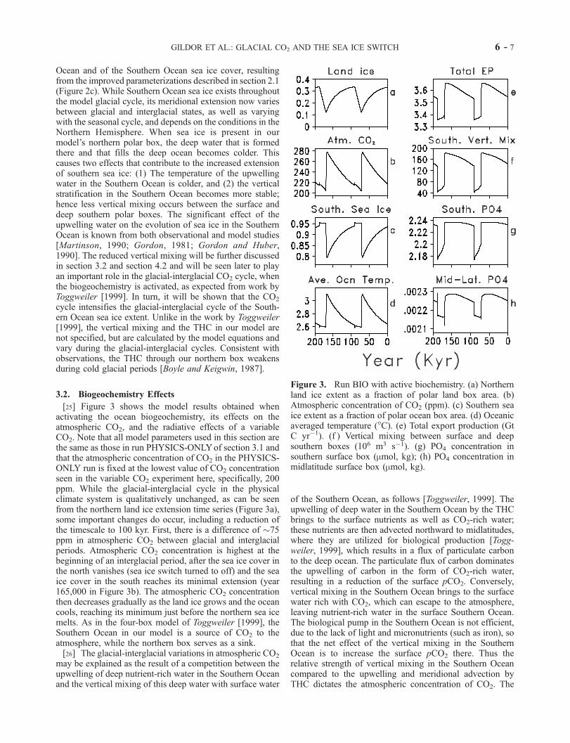
[25] Figure 3 shows the model results obtained whenactivating the ocean biogeochemistry, its effects on theatmospheric CO2, and the radiative effects of a variableCO2. Note that all model parameters used in this section arethe same as those in run PHYSICS-ONLYof section 3.1 andthat the atmospheric concentration of CO2 in the PHYSICS-ONLY run is fixed at the lowest value of CO2 concentrationseen in the variable CO2 experiment here, specifically, 200ppm. While the glacial-interglacial cycle in the physicalclimate system is qualitatively unchanged, as can be seenfrom the northern land ice extension time series (Figure 3a),some important changes do occur, including a reduction ofthe timescale to 100 kyr. First, there is a difference of �75ppm in atmospheric CO2 between glacial and interglacialperiods. Atmospheric CO2 concentration is highest at thebeginning of an interglacial period, after the sea ice cover inthe north vanishes (sea ice switch turned to off) and the seaice cover in the south reaches its minimal extension (year165,000 in Figure 3b). The atmospheric CO2 concentrationthen decreases gradually as the land ice grows and the oceancools, reaching its minimum just before the northern sea icemelts. As in the four-box model of Toggweiler [1999], theSouthern Ocean in our model is a source of CO2 to theatmosphere, while the northern box serves as a sink.[26] The glacial-interglacial variations in atmospheric CO2

may be explained as the result of a competition between theupwelling of deep nutrient-rich water in the Southern Oceanand the vertical mixing of this deep water with surface water

of the Southern Ocean, as follows [Toggweiler, 1999]. Theupwelling of deep water in the Southern Ocean by the THCbrings to the surface nutrients as well as CO2-rich water;these nutrients are then advected northward to midlatitudes,where they are utilized for biological production [Togg-weiler, 1999], which results in a flux of particulate carbonto the deep ocean. The particulate flux of carbon dominatesthe upwelling of carbon in the form of CO2-rich water,resulting in a reduction of the surface pCO2. Conversely,vertical mixing in the Southern Ocean brings to the surfacewater rich with CO2, which can escape to the atmosphere,leaving nutrient-rich water in the surface Southern Ocean.The biological pump in the Southern Ocean is not efficient,due to the lack of light and micronutrients (such as iron), sothat the net effect of the vertical mixing in the SouthernOcean is to increase the surface pCO2 there. Thus therelative strength of vertical mixing in the Southern Oceancompared to the upwelling and meridional advection byTHC dictates the atmospheric concentration of CO2. The

Figure 3. Run BIO with active biochemistry. (a) Northernland ice extent as a fraction of polar land box area. (b)Atmospheric concentration of CO2 (ppm). (c) Southern seaice extent as a fraction of polar ocean box area. (d) Oceanicaveraged temperature (�C). (e) Total export production (GtC yr�1). (f ) Vertical mixing between surface and deepsouthern boxes (106 m3 s�1). (g) PO4 concentration insouthern surface box (mmol, kg); (h) PO4 concentration inmidlatitude surface box (mmol, kg).


reduced rate of vertical mixing during glacial times allowsless CO2 from the deep water to escape into the atmosphereand results in a reduced atmospheric CO2.[27] The vertical mixing changes in the Southern Ocean

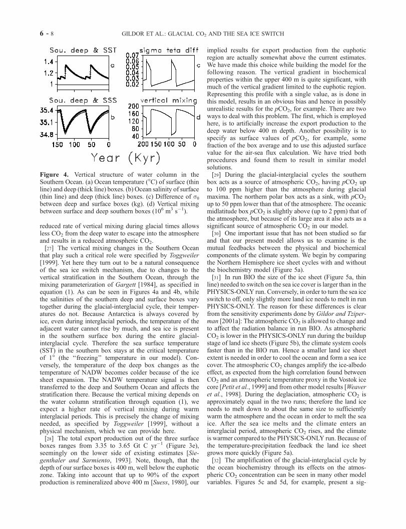
that play such a critical role were specified by Toggweiler[1999]. Yet here they turn out to be a natural consequenceof the sea ice switch mechanism, due to changes to thevertical stratification in the Southern Ocean, through themixing parameterization of Gargett [1984], as specified inequation (1). As can be seen in Figures 4a and 4b, whilethe salinities of the southern deep and surface boxes varytogether during the glacial-interglacial cycle, their temper-atures do not. Because Antarctica is always covered byice, even during interglacial periods, the temperature of theadjacent water cannot rise by much, and sea ice is presentin the southern surface box during the entire glacial-interglacial cycle. Therefore the sea surface temperature(SST) in the southern box stays at the critical temperatureof 1� (the ‘‘freezing’’ temperature in our model). Con-versely, the temperature of the deep box changes as thetemperature of NADW becomes colder because of the icesheet expansion. The NADW temperature signal is thentransferred to the deep and Southern Ocean and affects thestratification there. Because the vertical mixing depends onthe water column stratification through equation (1), weexpect a higher rate of vertical mixing during warminterglacial periods. This is precisely the change of mixingneeded, as specified by Toggweiler [1999], without aphysical mechanism, which we can provide here.[28] The total export production out of the three surface

boxes ranges from 3.35 to 3.65 Gt C yr�1 (Figure 3e),seemingly on the lower side of existing estimates [Sie-genthaler and Sarmiento, 1993]. Note, though, that thedepth of our surface boxes is 400 m, well below the euphoticzone. Taking into account that up to 90% of the exportproduction is remineralized above 400 m [Suess, 1980], our

implied results for export production from the euphoticregion are actually somewhat above the current estimates.We have made this choice while building the model for thefollowing reason. The vertical gradient in biochemicalproperties within the upper 400 m is quite significant, withmuch of the vertical gradient limited to the euphotic region.Representing this profile with a single value, as is done inthis model, results in an obvious bias and hence in possiblyunrealistic results for the pCO2, for example. There are twoways to deal with this problem. The first, which is employedhere, is to artificially increase the export production to thedeep water below 400 m depth. Another possibility is tospecify as surface values of pCO2, for example, somefraction of the box average and to use this adjusted surfacevalue for the air-sea flux calculation. We have tried bothprocedures and found them to result in similar modelsolutions.[29] During the glacial-interglacial cycles the southern

box acts as a source of atmospheric CO2, having pCO2 upto 100 ppm higher than the atmosphere during glacialmaxima. The northern polar box acts as a sink, with pCO2

up to 50 ppm lower than that of the atmosphere. The oceanicmidlatitude box pCO2 is slightly above (up to 2 ppm) that ofthe atmosphere, but because of its large area it also acts as asignificant source of atmospheric CO2 in our model.[30] One important issue that has not been studied so far

and that our present model allows us to examine is themutual feedbacks between the physical and biochemicalcomponents of the climate system. We begin by comparingthe Northern Hemisphere ice sheet cycles with and withoutthe biochemistry model (Figure 5a).[31] In run BIO the size of the ice sheet (Figure 5a, thin

line) needed to switch on the sea ice cover is larger than in thePHYSICS-ONLY run. Conversely, in order to turn the sea iceswitch to off, only slightly more land ice needs to melt in runPHYSICS-ONLY. The reason for these differences is clearfrom the sensitivity experiments done by Gildor and Tziper-man [2001a]: The atmospheric CO2 is allowed to change andto affect the radiation balance in run BIO. As atmosphericCO2 is lower in the PHYSICS-ONLY run during the buildupstage of land ice sheets (Figure 5b), the climate system coolsfaster than in the BIO run. Hence a smaller land ice sheetextent is needed in order to cool the ocean and form a sea icecover. The atmospheric CO2 changes amplify the ice-albedoeffect, as expected from the high correlation found betweenCO2 and an atmospheric temperature proxy in the Vostok icecore [Petit et al., 1999] and from other model results [Weaveret al., 1998]. During the deglaciation, atmospheric CO2 isapproximately equal in the two runs; therefore the land iceneeds to melt down to about the same size to sufficientlywarm the atmosphere and the ocean in order to melt the seaice. After the sea ice melts and the climate enters aninterglacial period, atmospheric CO2 rises, and the climateis warmer compared to the PHYSICS-ONLY run. Because ofthe temperature-precipitation feedback the land ice sheetgrows more quickly (Figure 5a).[32] The amplification of the glacial-interglacial cycle by

the ocean biochemistry through its effects on the atmos-pheric CO2 concentration can be seen in many other modelvariables. Figures 5c and 5d, for example, present a sig-

Figure 4. Vertical structure of water column in theSouthern Ocean. (a) Ocean temperature (�C) of surface (thinline) and deep (thick line) boxes. (b) Ocean salinity of surface(thin line) and deep (thick line) boxes. (c) Difference of sqbetween deep and surface boxes (kg). (d) Vertical mixingbetween surface and deep southern boxes (106 m3 s�1).


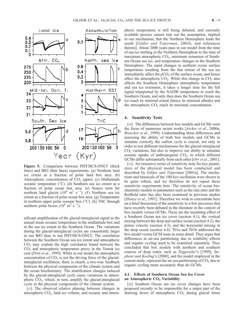
nificant amplification of the glacial-interglacial signal in theannual mean oceanic temperature in the midlatitude box andin the sea ice extent in the Southern Ocean. The variationsduring the glacial-interglacial cycles are consistently largerin run BIO than in run PHYSICS-ONLY. The correlationbetween the Southern Ocean sea ice extent and atmosphericCO2 may explain the high correlation found between theCO2 and atmospheric temperature proxy in the Vostok icecore [Petit et al., 1999]. While in our model the atmosphericconcentration of CO2 is not the driving force of the glacial-interglacial oscillation, there is clearly a two-way feedbackbetween the physical components of the climate system andthe ocean biochemistry: The stratification changes inducedby the glacial-interglacial cycle cause variations in atmos-pheric CO2, which, in turn, amplify the glacial-interglacialcycle in the physical components of the climate system.[33] The observed relative phasing between changes in

atmospheric CO2, land ice volume, and oceanic and atmos-

pheric temperature is still being debated, and currentlyavailable proxies cannot rule out the assumption, impliedin our mechanism, that the Northern Hemisphere leads thesouth [Gildor and Tziperman, 2001b, and referencestherein]. About 2000 years pass in our model from the timeof sea ice melting in the Northern Hemisphere to the time ofmaximum atmospheric CO2, minimum extension of South-ern Ocean sea ice, and temperature changes in the SouthernHemisphere. The rapid changes in northern ocean surfacetemperature resulting from the fast retreat of the sea iceimmediately affect the pCO2 of the surface ocean, and henceaffect the atmospheric CO2. While this change in CO2 alsoaffects the Southern Hemisphere atmospheric temperatureand sea ice extension, it takes a longer time for the fullsignal transported by the NADW temperature to reach theSouthern Ocean, and only then does the Southern Ocean seaice reach its minimal extent (hence its minimal albedo) andthe atmospheric CO2 reach its maximal concentration.

4. Sensitivity Tests

[34] The differences between box models and GCMs werethe focus of numerous recent works [Archer et al., 2000a;Broecker et al., 1999]. Understanding these differences andassessing the ability of both box models and GCMs tosimulate correctly the carbon cycle is crucial, not only inorder to test different mechanisms for the glacial-interglacialCO2 variations, but also to improve our ability to simulateoceanic uptake of anthropogenic CO2, in which differentGCMs differ substantially from each other [Orr et al., 2001].[35] An extensive series of sensitivity tests for key param-

eters of the physical model has been conducted anddescribed by Gildor and Tziperman [2001a]. The mecha-nism and timescale of the 100-kyr oscillation were shown tobe quite robust, and we therefore do not repeat thesesensitivity experiments here. The sensitivity of ocean bio-chemistry models to parameters such as the rain ratio and theRedfield ratio has also been examined in previous studies[Heinze et al., 1991]. Therefore we wish to concentrate hereon a brief discussion of the sensitivity to a few processes thathave recently been debated in the literature in the context ofbox models versus GCMs. These are the insulating effect ofa Southern Ocean sea ice cover (section 4.1), the verticalmixing between the deep and surface ocean (section 4.2), thepiston velocity (section 4.3), and the horizontal mixing inthe deep ocean (section 4.4). T01a and T01b addressed thebox model versus GCM issue in some detail. They argue thatdifferences in air-sea partitioning due to solubility effectsand organic cycling need to be examined separately. Theyconcluded that box models with northern and southernsources of deep water, such as Toggweiler’s [1999], Ste-phens and Keeling’s [2000], and the model employed in thecurrent study, represent the air-sea partitioning of CO2 due toorganic cycling more accurately than do GCMs.

4.1. Effects of Southern Ocean Sea Ice Coveron Atmospheric CO2 Variability

[36] Southern Ocean sea ice cover changes have beenproposed recently to be responsible for a major part of thedrawing down of atmospheric CO2 during glacial times

Figure 5. Comparison between PHYSICS-ONLY (thicklines) and BIO (thin lines) experiments. (a) Northern landice extent as a fraction of polar land box area. (b)Atmospheric concentration of CO2 (ppm). (c) Midlatitudeoceanic temperature (�C). (d) Southern sea ice extent as afraction of polar ocean box area. (e) Source term fornorthern land glacier (106 m3 s�1). (f ) Northern sea iceextent as a fraction of polar ocean box area. (g) Temperaturein northern upper polar oceanic box (�C). (h) THC throughnorthern polar boxes (106 m3 s�1).


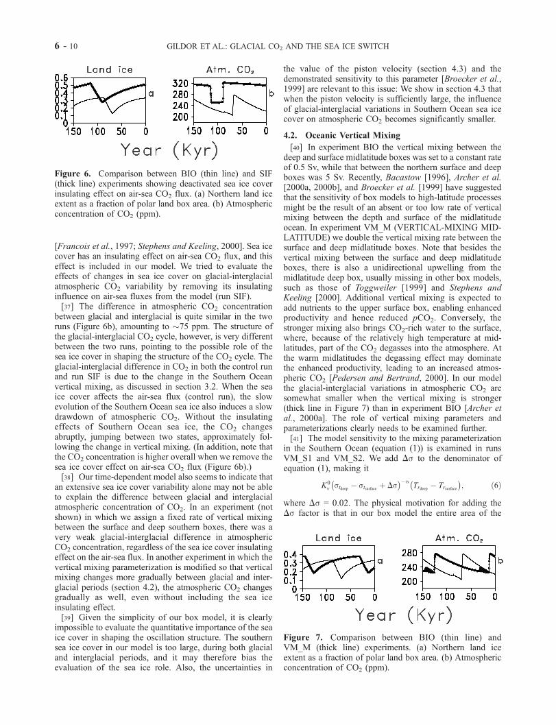
[Francois et al., 1997; Stephens and Keeling, 2000]. Sea icecover has an insulating effect on air-sea CO2 flux, and thiseffect is included in our model. We tried to evaluate theeffects of changes in sea ice cover on glacial-interglacialatmospheric CO2 variability by removing its insulatinginfluence on air-sea fluxes from the model (run SIF).[37] The difference in atmospheric CO2 concentration

between glacial and interglacial is quite similar in the tworuns (Figure 6b), amounting to �75 ppm. The structure ofthe glacial-interglacial CO2 cycle, however, is very differentbetween the two runs, pointing to the possible role of thesea ice cover in shaping the structure of the CO2 cycle. Theglacial-interglacial difference in CO2 in both the control runand run SIF is due to the change in the Southern Oceanvertical mixing, as discussed in section 3.2. When the seaice cover affects the air-sea flux (control run), the slowevolution of the Southern Ocean sea ice also induces a slowdrawdown of atmospheric CO2. Without the insulatingeffects of Southern Ocean sea ice, the CO2 changesabruptly, jumping between two states, approximately fol-lowing the change in vertical mixing. (In addition, note thatthe CO2 concentration is higher overall when we remove thesea ice cover effect on air-sea CO2 flux (Figure 6b).)[38] Our time-dependent model also seems to indicate that

an extensive sea ice cover variability alone may not be ableto explain the difference between glacial and interglacialatmospheric concentration of CO2. In an experiment (notshown) in which we assign a fixed rate of vertical mixingbetween the surface and deep southern boxes, there was avery weak glacial-interglacial difference in atmosphericCO2 concentration, regardless of the sea ice cover insulatingeffect on the air-sea flux. In another experiment in which thevertical mixing parameterization is modified so that verticalmixing changes more gradually between glacial and inter-glacial periods (section 4.2), the atmospheric CO2 changesgradually as well, even without including the sea iceinsulating effect.[39] Given the simplicity of our box model, it is clearly

impossible to evaluate the quantitative importance of the seaice cover in shaping the oscillation structure. The southernsea ice cover in our model is too large, during both glacialand interglacial periods, and it may therefore bias theevaluation of the sea ice role. Also, the uncertainties in

the value of the piston velocity (section 4.3) and thedemonstrated sensitivity to this parameter [Broecker et al.,1999] are relevant to this issue: We show in section 4.3 thatwhen the piston velocity is sufficiently large, the influenceof glacial-interglacial variations in Southern Ocean sea icecover on atmospheric CO2 becomes significantly smaller.

4.2. Oceanic Vertical Mixing

[40] In experiment BIO the vertical mixing between thedeep and surface midlatitude boxes was set to a constant rateof 0.5 Sv, while that between the northern surface and deepboxes was 5 Sv. Recently, Bacastow [1996], Archer et al.[2000a, 2000b], and Broecker et al. [1999] have suggestedthat the sensitivity of box models to high-latitude processesmight be the result of an absent or too low rate of verticalmixing between the depth and surface of the midlatitudeocean. In experiment VM_M (VERTICAL-MIXING MID-LATITUDE) we double the vertical mixing rate between thesurface and deep midlatitude boxes. Note that besides thevertical mixing between the surface and deep midlatitudeboxes, there is also a unidirectional upwelling from themidlatitude deep box, usually missing in other box models,such as those of Toggweiler [1999] and Stephens andKeeling [2000]. Additional vertical mixing is expected toadd nutrients to the upper surface box, enabling enhancedproductivity and hence reduced pCO2. Conversely, thestronger mixing also brings CO2-rich water to the surface,where, because of the relatively high temperature at mid-latitudes, part of the CO2 degasses into the atmosphere. Atthe warm midlatitudes the degassing effect may dominatethe enhanced productivity, leading to an increased atmos-pheric CO2 [Pedersen and Bertrand, 2000]. In our modelthe glacial-interglacial variations in atmospheric CO2 aresomewhat smaller when the vertical mixing is stronger(thick line in Figure 7) than in experiment BIO [Archer etal., 2000a]. The role of vertical mixing parameters andparameterizations clearly needs to be examined further.[41] The model sensitivity to the mixing parameterization

in the Southern Ocean (equation (1)) is examined in runsVM_S1 and VM_S2. We add Ds to the denominator ofequation (1), making it

K0v stdeep � stsurface þ Ds� ��a

Trdeep � Trsurface� �

; ð6Þ

where Ds = 0.02. The physical motivation for adding theDs factor is that in our box model the entire area of the

Figure 6. Comparison between BIO (thin line) and SIF(thick line) experiments showing deactivated sea ice coverinsulating effect on air-sea CO2 flux. (a) Northern land iceextent as a fraction of polar land box area. (b) Atmosphericconcentration of CO2 (ppm).

Figure 7. Comparison between BIO (thin line) andVM_M (thick line) experiments. (a) Northern land iceextent as a fraction of polar land box area. (b) Atmosphericconcentration of CO2 (ppm).


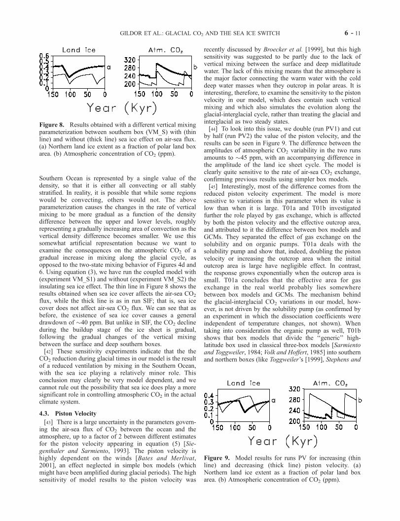
Southern Ocean is represented by a single value of thedensity, so that it is either all convecting or all stablystratified. In reality, it is possible that while some regionswould be convecting, others would not. The aboveparameterization causes the changes in the rate of verticalmixing to be more gradual as a function of the densitydifference between the upper and lower levels, roughlyrepresenting a gradually increasing area of convection as thevertical density difference becomes smaller. We use thissomewhat artificial representation because we want toexamine the consequences on the atmospheric CO2 of agradual increase in mixing along the glacial cycle, asopposed to the two-state mixing behavior of Figures 4d and6. Using equation (3), we have run the coupled model with(experiment VM_S1) and without (experiment VM_S2) theinsulating sea ice effect. The thin line in Figure 8 shows theresults obtained when sea ice cover affects the air-sea CO2

flux, while the thick line is as in run SIF; that is, sea icecover does not affect air-sea CO2 flux. We can see that asbefore, the existence of sea ice cover causes a generaldrawdown of �40 ppm. But unlike in SIF, the CO2 declineduring the buildup stage of the ice sheet is gradual,following the gradual changes of the vertical mixingbetween the surface and deep southern boxes.[42] These sensitivity experiments indicate that the the

CO2 reduction during glacial times in our model is the resultof a reduced ventilation by mixing in the Southern Ocean,with the sea ice playing a relatively minor role. Thisconclusion may clearly be very model dependent, and wecannot rule out the possibility that sea ice does play a moresignificant role in controlling atmospheric CO2 in the actualclimate system.

4.3. Piston Velocity

[43] There is a large uncertainty in the parameters govern-ing the air-sea flux of CO2 between the ocean and theatmosphere, up to a factor of 2 between different estimatesfor the piston velocity appearing in equation (5) [Sie-genthaler and Sarmiento, 1993]. The piston velocity ishighly dependent on the winds [Bates and Merlivat,2001], an effect neglected in simple box models (whichmight have been amplified during glacial periods). The highsensitivity of model results to the piston velocity was

recently discussed by Broecker et al. [1999], but this highsensitivity was suggested to be partly due to the lack ofvertical mixing between the surface and deep midlatitudewater. The lack of this mixing means that the atmosphere isthe major factor connecting the warm water with the colddeep water masses when they outcrop in polar areas. It isinteresting, therefore, to examine the sensitivity to the pistonvelocity in our model, which does contain such verticalmixing and which also simulates the evolution along theglacial-interglacial cycle, rather than treating the glacial andinterglacial as two steady states.[44] To look into this issue, we double (run PV1) and cut

by half (run PV2) the value of the piston velocity, and theresults can be seen in Figure 9. The difference between theamplitudes of atmospheric CO2 variability in the two runsamounts to �45 ppm, with an accompanying difference inthe amplitude of the land ice sheet cycle. The model isclearly quite sensitive to the rate of air-sea CO2 exchange,confirming previous results using simpler box models.[45] Interestingly, most of the difference comes from the

reduced piston velocity experiment. The model is moresensitive to variations in this parameter when its value islow than when it is large. T01a and T01b investigatedfurther the role played by gas exchange, which is affectedby both the piston velocity and the effective outcrop area,and attributed to it the difference between box models andGCMs. They separated the effect of gas exchange on thesolubility and on organic pumps. T01a deals with thesolubility pump and show that, indeed, doubling the pistonvelocity or increasing the outcrop area when the initialoutcrop area is large have negligible effect. In contrast,the response grows exponentially when the outcrop area issmall. T01a concludes that the effective area for gasexchange in the real world probably lies somewherebetween box models and GCMs. The mechanism behindthe glacial-interglacial CO2 variations in our model, how-ever, is not driven by the solubility pump (as confirmed byan experiment in which the dissociation coefficients wereindependent of temperature changes, not shown). Whentaking into consideration the organic pump as well, T01bshows that box models that divide the ‘‘generic’’ high-latitude box used in classical three-box models [Sarmientoand Toggweiler, 1984; Volk and Hoffert, 1985] into southernand northern boxes (like Toggweiler’s [1999], Stephens and

Figure 8. Results obtained with a different vertical mixingparameterization between southern box (VM_S) with (thinline) and without (thick line) sea ice effect on air-sea flux.(a) Northern land ice extent as a fraction of polar land boxarea. (b) Atmospheric concentration of CO2 (ppm).

Figure 9. Model results for runs PV for increasing (thinline) and decreasing (thick line) piston velocity. (a)Northern land ice extent as a fraction of polar land boxarea. (b) Atmospheric concentration of CO2 (ppm).


Keeling’s [2000], and the model used in this study) seem todo better than GCMs. Certainly, the sensitivity to the pistonvelocity and the effective area for gas exchange should befurther examined.

4.4. Horizontal Mixing in the Deep Ocean

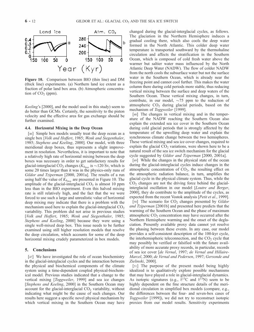
[46] Simple box models usually treat the deep ocean as asingle box [Volk and Hoffert, 1985; Wenk and Siegenthaler,1985; Stephens and Keeling, 2000]. Our model, with threemeridional deep boxes, thus represents a slight improve-ment in resolution. Nevertheless, it is important to note thata relatively high rate of horizontal mixing between the deepboxes was necessary in order to get satisfactory results forglacial-interglacial CO2 changes (Khdeep is �120 Sv, which issome 20 times larger than it was in the physics-only runs ofGildor and Tziperman [2000, 2001a]. The results of a runusing half the value of Khdeep are presented in Figure 10. Theamplitude of the glacial-interglacial CO2 is almost 10 ppmless than in the BIO experiment. Even this halved mixingrate is still relatively high, and the fact that the we wereforced to use such a large and unrealistic value of horizontaldeep mixing may indicate that there is a problem with themechanism used here to explain the glacial-interglacial CO2

variability. This problem did not arise in previous studies[Volk and Hoffert, 1985; Wenk and Siegenthaler, 1985;Stephens and Keeling, 2000] because they were using asingle well-mixed deep box. This issue needs to be furtherexamined using still higher resolution models that resolvethe deep circulation, which accounts for some of the deephorizontal mixing crudely parameterized in box models.

5. Conclusions

[47] We have investigated the role of ocean biochemistryin the glacial-interglacial cycles and the interaction betweenthe physical and biochemical components of the climatesystem using a time-dependent coupled physical-biochem-ical model. Previous studies indicated that a change to thevertical mixing [Toggweiler, 1999] and sea ice changes[Stephens and Keeling, 2000] in the Southern Ocean mayaccount for the glacial-interglacial CO2 variability, withoutindicating what might be the cause of such changes. Ourresults here suggest a specific novel physical mechanism bywhich vertical mixing in the Southern Ocean may have

changed during the glacial-interglacial cycles, as follows.The glaciation in the Northern Hemisphere induces agradual cooling there, which also cools the deep waterformed in the North Atlantic. This colder deep watertemperature is transported southward by the thermohalinecirculation and affects the stratification in the SouthernOcean, which is composed of cold fresh water above thewarmer but saltier water mass influenced by the NorthAtlantic Deep Water (NADW). The flow of colder NADWfrom the north cools the subsurface water but not the surfacewater in the Southern Ocean, which is already near thefreezing point and cannot cool further. This makes the watercolumn there during cold periods more stable, thus reducingvertical mixing between the surface and deep waters of theSouthern Ocean. These vertical mixing changes, in turn,contribute, in our model, �75 ppm to the reduction ofatmospheric CO2 during glacial periods, based on themechanism of Toggweiler [1999].[48] The changes in vertical mixing and in the temper-

ature of the NADW reaching the Southern Ocean alsoexplain the extended sea ice cover in the Southern Oceanduring cold glacial periods that is strongly affected by thetemperature of the upwelling deep water and explain thesynchronous climate change between the two hemispheres.These vertical mixing and sea ice cover changes, required toexplain the glacial CO2 variations, were shown here to be anatural result of the sea ice switch mechanism for the glacialcycle suggested by Gildor and Tziperman [2000, 2001a].[49] While the changes in the physical state of the ocean

during the glacial-interglacial cycles induce changes in theatmospheric concentration of CO2, the resulting effect onthe atmospheric radiation balance, in turn, amplifies theglacial cycle in the physical climate system. Thus, while theCO2 changes are not the driving force behind the glacial-interglacial oscillation in our model [Loutre and Berger,2000], they do contribute to the amplitude of the cycles, asexpected from the recent Vostok analysis [Petit et al., 1999].[50] The scenario for CO2 changes presented by Gildor

and Tziperman [2001b] and presented here predicts that thewarming of the Southern Ocean and the phase of maximumatmospheric CO2 concentration may have occurred after theNorthern Hemisphere warming and the onset of the degla-ciation. Presently available proxy data cannot yet resolvethe phasing between these events. In any case, our modelprovides a self-consistent description of the 100-kyr cycle,the interhemispheric teleconnection, and the CO2 cycle thatmay possibly be verified or falsified with the future avail-ability of more accurate proxy records, in particular, recordsof sea ice cover [de Vernal, 1997; de Vernal and Hillaire-Marcel, 2000; de Vernal and Pedersen, 1997; Gersonde andZielinski, 2000].[51] The purpose of the present model being highly

idealized is to qualitatively explore possible mechanismsthat may have played a role in glacial-interglacial dynamics.As isotopic signatures (e.g., d13C and d15N) seem to behighly dependent on the fine structure details of the meri-dional circulation in simplified box models (compare, e.g.,the differences between the four- and seven-box cases ofToggweiler [1999]), we did not try to reconstruct isotopicproxies from our model results. Sensitivity experiments

Figure 10. Comparison between BIO (thin line) and DM(thick line) experiments. (a) Northern land ice extent as afraction of polar land box area. (b) Atmospheric concentra-tion of CO2 (ppm).


demonstrate that our results are generally robust, but furtherinvestigation is required, especially regarding the role ofpiston velocity and deep horizontal mixing. Recent works(T01a and T01b) confirmed that there is a strong sensitivityto gas exchange and polar area. Despite our model’slimitations, we feel that the results are at least plausibleand can explain some of the main aspects of both thephysical and biochemical glacial oscillations.[52] Other processes not included in our model, such as

alkalinity changes, have certainly contributed to theobserved atmospheric CO2 cycles. We have used a constantRedfield ratio, although recent observations in the SouthernOcean show that depending on the local stratification,different phytoplankton species with different Redfieldratios may dominate [Arrigo et al., 1999]. The resultingchanges in the Redfield ratio can be >50%, with the higherC/P ratio species being dominant in less stratified water[Arrigo et al., 1999]. Our model predicts a more stablestratification in the Southern Ocean during glacial maxi-mum but a less stably stratified ocean in the midlatitudes, asthe surface ocean there has cooled more than the deepocean. Additional contribution to the drawdown of atmos-pheric CO2 during glacial times might have arisen, had theRedfield ratio at midlatitudes changed during the glacialcycles due to these midlatitude stratification changes basedon a similar mechanism as observed in higher latitudes byArrigo et al. [1999]. Our main result is the possible physicalmechanism resulting in vertical mixing and sea ice coverchanges in the Southern Ocean, and it would be mostinteresting to see this mechanism examined using fullergeneral circulation models and new proxy data.

[53] Acknowledgments. This work is partially supported by theIsraeli-U.S. Binational Science Foundation.

ReferencesArcher, D., G. Eshel, A. Winguth, W. Broecker, R. Pierrehumbert, M.Tobis, and R. Jacob, Atmospheric pCO2 sensitivity to the biologicalpump in the ocean, Global Biogeochem. Cycles, 14, 1219–1230, 2000a.

Archer, D., A. Winguth, D. Lea, and N. Mahowald, What caused theglacial/interglacial atmospheric pCO2 cycles?, Rev. Geophys., 38, 159–189, 2000b.

Arrigo, K. R., D. H. Robinson, D. L. Worthen, R. B. Dunbar, G. R. Di-Tullio, M. VanWoert, and M. P. Lizotte, Phytoplankton community struc-ture and the drawdown of nutrients and CO2 in the Southern Ocean,Science, 283, 365–367, 1999.

Bacastow, R., The effect of temperature change of the warm surface watersof the ocean on atmospheric CO2, Global Biogeochem. Cycles, 10, 319–333, 1996.

Bacastow, R., and E. Maier-Reimer, Ocean circulation model of the carboncycle, Clim. Dyn., 4, 95–125, 1990.

Bates, N., and L. Merlivat, The influence of short-term wind variability onair-sea CO2 exchange, Geophys. Res. Lett., 28, 3281–3284, 2001.

Boyle, E. A., and L. Keigwin, North Atlantic thermohaline circulationduring the past 20,000 years linked to high-latitude surface temperature,Nature, 330, 35–40, 1987.

Broecker, W., J. Lynch-Stieglitz, D. Archer, M. Hofmann, E. Maier-Reimer,O. Marchal, T. Stocker, and N. Gruber, How strong is the Harvadton-Bearconstraint?, Global Biogeochem. Cycles, 13, 817–820, 1999.

Crosta, X., J. Pichon, and L. Burckle, Application of modern analog tech-nique to marine Antarctic diatoms: Reconstruction of maximum sea iceextent at the Last Glacial Maximum, Paleoceanography, 13, 284–297,1998.

Dansgaard, W., J. White, and S. Johnsen, The abrupt termination of theYounger Dryas climate event, Nature, 339, 532–534, 1989.

Daskal Hausman, E., and M. B. McElroy, Role of sea surface temperatureand ocean circulation changes in the reorganization of the global carbon

cycle at the last glacial termination, Global Biogeochem. Cycles, 13,371–381, 1999.

de Vernal, A., Sea-surface conditions in the northwest North Atlantic duringthe Last Glacial Maximum, GEOTOP contrib. 97-001, Cent. for Res. inIsotopic Geochem. and Geochronol., Univ. of Quebec, Montreal, Que.,Canada, 1997. (Available at http://www.unites.uqam.ca/geotop/18ka.html)

de Vernal, A., and C. Hillaire-Marcel, Sea-ice cover, sea-surface salinityand halo/thermo-cline structure of the northwest North Atlantic: Modernversus full glacial condition, Quater. Res., 19, 65–85, 2000.

de Vernal, A., and T. F. Pedersen, Micropaleontology and palynology ofcore par87a-10: A 23,000 year record of paleoenvironmental changes inthe Gulf of Alaska, northeast North Pacific, Paleoceanography, 12, 821–830, 1997.

Francois, R., M. A. Altabet, E. Yu, D. M. Sigman, M. P. Bacon, M. Frank,G. Bohrmann, G. Bareille, and L. D. Labeyrie, Contribution of SouthernOcean surface-water stratification to low atmospheric CO2 concentrationsduring the last glacial period, Nature, 389, 929–935, 1997.

Ganopolski, S., A. Rahmstorf, V. Petoukhov, and M. Claussen, Simulationof modern and glacial climates with a coupled global model of inter-mediate complexity, Nature, 391, 351–356, 1998.

Gargett, A., Vertical eddy diffusivity in the ocean interior, J. Mar. Res., 42,359–393, 1984.

Gersonde, R., and U. Zielinski, The reconstruction of late quaternary Ant-arctic sea-ice distribution: The use of diatoms as a proxy for sea-ice,Paleogeogr. Paleoclimatol. Paleoecol., 162, 263–286, 2000.

Ghil, M., Cryothermodynamics: The chaotic dynamics of paleoclimate,Physica D, 77, 130–159, 1994.

Ghil, M., A. Mulhaupt, and P. Pestiaux, Deep water formations and Qua-ternary glaciations, Clim. Dyn., 2, 1–10, 1987.

Gildor, H., and E. Tziperman, Sea ice as the glacial cycles climate switch:Role of seasonal and Milankovitch solar forcing, Paleoceanography, 15,605–615, 2000.

Gildor, H., and E. Tziperman, A sea ice climate switch mechanism for the100-kyr glacial cycles, J. Geophys. Res., 106, 9117–9133, 2001a.

Gildor, H., and E. Tziperman, Physical mechanisms behind biogeochemicalglacial-interglacial CO2 variations, Geophys. Res. Lett., 28, 2421–2424,2001b.

Gnanadesikan, A., A simple predictive model for the structure of the ocea-nic pycnocline, Science, 283, 2077–2079, 1999.

Gordon, A., Seasonality of Southern Ocean sea ice, J. Geophys. Res., 86,4193–4197, 1981.

Gordon, A., and B. Huber, Southern Ocean winter mixed layer, J. Geophys.Res., 95, 11,655–11,672, 1990.

Heinze, C., E. Maier-Reimer, and K. Winn, Glacial pCO2 reduction by theworld ocean: Experiments with the Hamburg carbon model, Paleoceano-graphy, 4, 395–430, 1991.

Kallen, E., C. Crafoord, and M. Ghil, Free oscillations in a climate modelwith ice-sheet dynamics, J. Atmos. Sci., 36, 2292–2303, 1979.

Loutre, M., and A. Berger, No glacial-interglacial cycle in the ice volumesimulated under a constant astronomical forcing and a variable CO2,Geophys. Res. Lett., 27, 783–786, 2000.

Maier-Reimer, E., Geochemical cycles in an ocean general circulation mod-el: Preindustrial tracer distribution, Global Biogeochem. Cycles, 7, 645–677, 1993.

Martinson, D., Evolution of the Southern Ocean winter mixed layer and seaice: Open ocean deepwater formation and ventilation, J. Geophys. Res.,95, 11,641–11,654, 1990.

Matsumoto, K., and J. Lynch-Stieglitz, Similar glacial and holocene deepwater circulation inferred from southeast Pacific benthic foraminiferalcarbon isotope composition, Paleoceanography, 14, 149–163, 1999.

Maykut, G., and D. Perovich, The role of shortwave radiation in sum-mer decay of a sea ice cover, J. Geophys. Res., 92, 7032–7044,1987.

Orr, J., et al., Estimates of anthropogenic carbon uptake from four three-dimensional global ocean models, Global Biogeochem. Cycles, 15, 43–60, 2001.

Pedersen, T., and P. Bertrand, Influence of oceanic rheostats and amplifierson atmopsheric CO2 content during the late Quaternary, Quat. Sci. Rev.,19, 273–283, 2000.

Petit, J. R., et al., Climate and atmospheric history of the past 420,000 yearsfrom the Vostok ice core, Antarctica, Nature, 399, 429–436, 1999.

Ramanathan, V., et al., Climate-chemical interaction and effects of changingatmospheric trace gases, Rev. Geophys., 25, 1441–1482, 1987.

Sarmiento, J. L., and J. R. Toggweiler, A new model for the role of theoceans in determining atmospheric pCO2, Nature, 308, 621–624,1984.

Schrag, D., G. Hampt, and D. Murray, Pore fluid constraints on the tem-


perature and oxygen isotopic composition of the glacial ocean, Science,272, 1930–1932, 1996.

Siegenthaler, U., and J. Sarmiento, Atmospheric carbon dioxide and theocean, Nature, 365, 119–125, 1993.

Sigman, D. M., and E. A. Boyle, Glacial/interglacial variations in atmo-spheric carbon dioxide, Nature, 407, 859–869, 2000.

Sikes, E. L., C. R. Samson, T. P. Guilderson, and W. R. Howard, Oldradiocarbon ages in the southwest Pacific Ocean during the last glacialperiod and deglaciation, Nature, 405, 555–559, 2000.

Stephens, B. B., and R. Keeling, The influence of Antarctic sea ice onglacial-interglacial CO2 variations, Nature, 404, 171–174, 2000.

Stommel, H., Thermohaline convection with two stable regimes of flow,Tellus, 13, 224–230, 1961.

Suess, E., Particulate organic carbon flux in the oceans: Surface and oxygenutilization, Nature, 288, 260–262, 1980.

Toggweiler, J. R., Variation of atmospheric CO2 by ventilation of theocean’s deepest water, Paleoceanography, 14, 572–588, 1999.

Toggweiler, J. R., and B. Samuels, Is the magnitude of the deep outflowfrom the Atlantic Ocean actually governed by the Southern Hemispherewinds?, in The Global Carbon Cycle, NATO ASI Ser. 1, vol. 15, edited byM. Heimann, pp. 303–331, Springer-Verlag, New York, 1993.

U.N. Educational, Scientific, and Cultural Organization, Tenth report of theJoint Panel on Oceanographic Tables and Standards, Tech. Rep., 36,Paris, 1981.

Volk, T., and M. Hoffert, Ocean carbon pumps: Analysis of relativestrengths and efficiencies in ocean-driven atmospheric CO2 changes, inThe Carbon Cycle and Atmospheric CO2: Natural Variations Archean to

Present, Geophys. Monogr. Ser., vol. 32, edited by E. T. Sundquist and W.S. Broecker, pp. 99–110, AGU, Washington, D. C., 1985.

Weaver, A. J., M. Eby, A. Fanning, and E. C. Wiebe, Simulated influence ofcarbon dioxide, orbital forcing and ice sheets on the climate of the LastGlacial Maximum, Nature, 394, 847–853, 1998.

Weertman, J., Milankovitch solar radiation variations and ice age ice sheetsizes, Nature, 261, 17–20, 1976.

Wenk, T., and U. Siegenthaler, The high-latitude ocean as a control ofatmospheric CO2, in The Carbon Cycle and Atmospheric CO2: NaturalVariations Archean to Present, Geophys. Monogr. Ser., vol. 32, edited byE. T. Sundquist and W. S. Broecker, pp. 185–194, AGU, Washington,D. C., 1985.

Yamanaka, Y., Development of ocean biogeochemical general circulationmodel, Tech. Rep. 1, Cent. for Clim. Sys. Res., Univ. of Tokyo, Tokyo,1996.

Yu, E.-F., R. Francois, and M. P. Bacon, Similar rates of modern and last-glacial ocean thermohaline circulation inferred from radio-chemical data,Nature, 379, 689–694, 1996.

��H. Gildor and E. Tziperman, Environmental Sciences, Weizmann

Institute of Science, Rehovot 76100, Israel. ([email protected];[email protected])J. R. Toggweiler, Geophysical Fluid Dynamics Laboratory, National

Oceanic and Atmospheric Administration, P.O. Box 308, Princeton, NJ08542, USA. ([email protected])


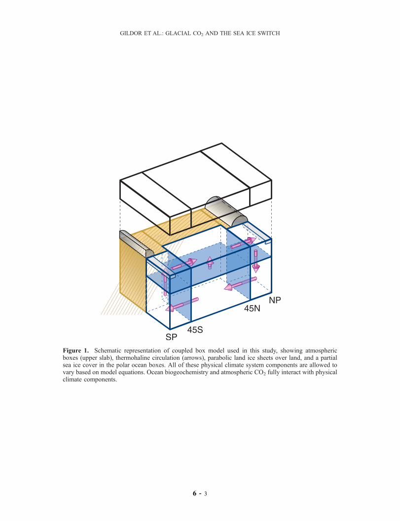
Figure 1. Schematic representation of coupled box model used in this study, showing atmosphericboxes (upper slab), thermohaline circulation (arrows), parabolic land ice sheets over land, and a partialsea ice cover in the polar ocean boxes. All of these physical climate system components are allowed tovary based on model equations. Ocean biogeochemistry and atmospheric CO2 fully interact with physicalclimate components.

GILDOR ET AL.: GLACIAL CO2 AND THE SEA ICE SWITCH

6 - 3

Documents

Sea ice switch mechanism and glacial-interglacial CO ... · Sea ice switch mechanism and glacial-interglacial CO ... In this proposed mechanism the glacial oscillations ... start