Embed Size (px)
Citation preview
| 467 |
| 60/3 |
RECE
NZIRA
NI ČL
ANKI
| PEE
R-RE
VIEW
ED AR
TICLE
S
VG 2
01
6
GEODETSKI VESTNIK | letn. / Vol. 60 | št. / No. 3 |
SI |
EN
residual effects in GPS observations, two-way nested classification, variance components estimation, integral approach, directions for further research
rezidualni učinki GPS-meritev, dvofaktorsko ugnezdene razvrstitve, ocena komponent disperzije, integralni pristop,
smernice za nadaljne raziskovanje
KEY WORDSKLJUČNE BESEDE
IZVLEČEK ABSTRACT Variance components analysis of residual errors remaining in the GPS double-difference phase observations is presented in this paper. These errors arise due to unmodeled ionospheric, tropospheric and multipath effects and limit the accuracy of n (northwards), e (eastwards) and u (upwards) coordinate estimates. In addition, there are unavoidable pure random errors. An integral approach to variance components estimation of the residual errors is presented herein. The mathematical basis of the approach lies in the two-way nested classification, where one uses a linear model with random effects. It turned out that, for a baseline of 40km in length at mid-latitude region and during a year of the lowest sunspot activity in the 11-year cycle, daily standard deviations estimates of combined tropospheric and ionospheric effects are with intervals of ~1–11mm, ~1–7mm and ~4–51mm for n, e and u coordinate, respectively. In the same order, for the multipath effects, the intervals are ~4–12mm, ~3–9mm and ~8–30mm, while with pure random error those are ~5–9mm, ~4–7mm and ~9–20mm. It is important to say that the highest values arise in summer and the lowest in winter period.
V prispevku prikazujemo analizo komponent variance nemodelranih pogreškov dvojnih faznih razlik GPS-meritev. Ti pogreški se pojavljajo zaradi nemodelnih ionosferskih, troposferskih vplivov in vplivov večpotja ter omejujejo točnost določitve koordinat. Poleg naštetega so meritve obremenjene z neizogibnimi slučajnimi pogreški. V prispevku predstavljamo integralen pristop ocene komponent variance nemodeliranih pogreškov opazovanj. Matematična osnova pristopa je dvofaktorska ugnezdena klasifikacija z uporabo linearnega modela za vhodne podatke, obremenjene s slučajnimi pogreški. Izkazalo se je, da so za en bazni vektor dolžine 40 kilometrov na območju srednjih geografskih širin, v letu z najnižjo Sončevo aktivnostjo znotraj 11-letnega obdobja, dnevne vrednosti standardnih odklonov skupnih vplivov troposfere in ionosfere v intervalih ~1–11 mm, ~1–7 mm in ~4–51 mm za koordinate n (proti severu), e (proti vzhodu) in u (navzgor), respektivno. Po istem zaporedju so intervali za večpotje ~4–12 mm, ~3–9 mm in ~8–30 mm, za slučajne pogreške pa v intervalih ~5–9 mm, ~4–7 mm in ~9–20 mm. Vrednosti standardnih odklonov so najvišje v poletnem, najnižje pa v zimskem obdobju.
DOI: 10.15292/geodetski-vestnik.2016.03.467-482SCIENTIFIC ARTICLEReceived: 10. 5. 2016Accepted: 14. 7. 2016
UDK: 550.8.08 Klasifikacija prispevka po COBISS.SI: 1.01
Prispelo: 10. 5. 2016Sprejeto: 14. 7. 2016
Darko Anđić
VARIANCE COMPONENTS ESTIMATION OF RESIDUAL ERRORS IN GPS PRECISE POSITIONING
OCENA KOMPONENT VARIANCE NEMODELIRANIH POGREŠKOV V NATANČNEM
POZICIONIRANJU GPS
Darko Anđić | OCENA KOMPONENT VARIANCE NEMODELIRANIH POGREŠKOV V NATANČNEM POZICIONIRANJU GPS | VARIANCE COMPONENTS ESTIMATION OF RESI-DUAL ERRORS IN GPS PRECISE POSITIONING | 467-482 |
| 468 || 468 || 468 |
| 60/3 | GEODETSKI VESTNIK
RECE
NZIRA
NI ČL
ANKI
| PEE
R-RE
VIEW
ED AR
TICLE
SSI
| EN
Darko Anđić | OCENA KOMPONENT VARIANCE NEMODELIRANIH POGREŠKOV V NATANČNEM POZICIONIRANJU GPS | VARIANCE COMPONENTS ESTIMATION OF RESI-DUAL ERRORS IN GPS PRECISE POSITIONING | 467-482 |
1 INTRODUCTION
The theoretical basis regarding mathematical models of GPS observations which are used in processing of those observations can be found in almost every publication considering GPS. Of importance for analysis in this paper is a residual part in the double-difference phase observations arising due to several unmodeled effects limiting accuracy of positioning. The residuals exist because of lack of knowledge of a representational mathematical model for their component effects with irregular behaviour in time. Namely, the time-variable residuals of errors stem from unmodeled errors due to signal multipath, as well as tropospheric and ionospheric refraction, are analysed herein (the characteristics of these three effects are shown in subsection 1.2). The fourth effect arises due to antenna phase center offset (APCO) and antenna phase center variations (APCV). Namely, the electrical antenna phase center varies with satellite elevation and azimuth, intensity of the satellite signal, and is also frequency dependent. So, each incoming signal has its own electrical antenna phase center. The APCO defines the difference between the geometrical point on the antenna denoted as antenna reference point (ARP) and the mean position of the electrical antenna phase center (MAPC). On the other side, the APCV arise due to differences between individual electrical antenna phase centers and the MAPC. Unmodeled errors due to antenna phase centre offset and variations which, otherwise, have the greatest impact on accuracy of the coor-dinate in vertical plane, will not be considered because in this paper one uses a GPS baseline of 40km in length with receivers and antennas of the same type at both its ends (see subsection 1.3), and when using antennas of the same type at short- and medium-distance baselines (<1000km), there is no need to introduce corrections, because in double-difference phase observation model the effects of antenna phase centre offsets and variations of both antennas will cancel out (Kouba, 2009; El-Hattab, 2013). Of course, the cancellation is possible only if the receivers do not loose lock during the GPS observation session, in which case we have absence of cycle slips.
Above mentioned residual effects, together with the unavoidable pure random errors (pure error), limit the accuracy of GPS positioning, i.e. the accuracy of three component relative coordinate estimates of the measured GPS baseline vector in a chosen reference system. For geodetic purposes, one often uses positions in north-south (coordinate n) and east-west direction (coordinate e) in the plane of the local coordinate system containing a point on the Earth surface where the reference GPS receiver is located. The plane is orthogonal to the ellipsoid (WGS84) normal in that point. The third coordinate (u) rep-resents orthogonal distance (upwards) between the point with the second GPS receiver (on the other side of the baseline) to the local horizon (the plane defined by n and e coordinate axes) of the reference receiver position (Leick, 2004).
Research in this paper aims to prove the possibility of using the two-way nested classification (sometimes also referred to as a hierarchical classification) linear model with random effects in variance components estimation of residuals arising due to the influence of multipath and combined influence of ionospheric and tropospheric refraction with simultaneous separation of the pure error variance estimate.
1.1 First results of the application of two-way nested classification in GPS positioning
In his doctoral dissertation, which is in its final stage, under the supervision of prof. D.Blagojević, the author of this paper presents the results of variance components researching regarding above mentioned
| 469 || 469 || 469 |
GEODETSKI VESTNIK | 60/3 |
RECE
NZIRA
NI ČL
ANKI
| PEE
R-RE
VIEW
ED AR
TICLE
SSI
| EN
Darko Anđić | OCENA KOMPONENT VARIANCE NEMODELIRANIH POGREŠKOV V NATANČNEM POZICIONIRANJU GPS | VARIANCE COMPONENTS ESTIMATION OF RESI-DUAL ERRORS IN GPS PRECISE POSITIONING | 467-482 |
dominant residual effects and pure random effects in GPS double-difference phase observables, their mutual correlations and behaviour. The research has been conducted by using a common linear model with the two-way nested classification providing an integral consideration of all of these effects and until now there have been no papers about it. It is important to note that the idea for such a research came from prof. G.Perović. Guided by that idea, using mathematical formulas for two-way nested classification analysis with random effects (Searle, 1971) and testing hypotheses about influence of those effects (Hald, 1957), the author of this paper applied relational theory on relative GPS coordinates in his doctoral dis-sertation, whereby he greatly expanded analysis, and the results of a small part of the research, by which applicability of the mentioned idea is provided, have been cited in later published monograph (Perović, 2015). In this way, the results of integral variance components estimation for multipath, combined tropospheric and ionospheric refraction and pure random effects for a chosen GPS baseline have been published for the first time. In the monograph, actually, the PERG2FH method incorporating those results has also been presented for the first time. However, there is an essential difference between the source presentation and that in the monograph. The difference relates to the fact that the author of the dissertation, as mentioned before, analysed multipath effect among residuals, while the results for vari-ance components he obtained have been presented by Perović (2015) as if they relate to quasi-stationary atmosphere blocks, whereby multipath effect has been rejected as if it does not exist.
In the dissertation, static GPS observations registered at each 30s over a period of four consecutive years (2008-2011) at two permanent stations of the (Montenegrin) MontePos network and eight EUREF permanent stations have been analysed. These stations were chosen so that they formed five GPS baselines with five different lengths, from 5.6km to 282km.
The behaviour of variance components estimates were separately analysed for daytime (when there was the strongest impact of ionosphere) and night (when the impact of ionosphere was reduced to a mini-mum), and the other relevant results were presented therein. Namely, the author has also dealt with a detailed research of the impact of outliers on the variance components estimates of residual and pure random components of the GPS station position error. Besides, the removal of the outliers has also been discussed as a part of this issue. The whole part of the research and most of the results obtained are planned to be presented in a particular paper dealing only with this issue. However, only a small part of the research is presented herein.
1.2 Main characteristics of the effects whose residuals are discussed in this paper
Multipath
Multipath is one of the most important error sources limiting GPS positioning accuracy and it is the most dominant when it comes to the baselines with smaller length. The phenomenon is conditioned by the receiver station environment characteristics. Due to periodic changes in the geometry of the positions of satellites, the influence of multipath changes with the same period, except in the case of the extraordinary, short-term circumstances. In order to discuss the two multipath components with completely different physical characteristics, the author presents the site dependent error. This error is composed of the errors coming from three effects, if the antenna setting instability error is omitted under the assumption of the high stability. So, in a simplified form it is written as δS = δPCV + δMPnear−field + δMPfar−field (Wübbena,
| 470 || 470 || 470 |
| 60/3 | GEODETSKI VESTNIK
RECE
NZIRA
NI ČL
ANKI
| PEE
R-RE
VIEW
ED AR
TICLE
SSI
| EN
Schmitz and Boettcher, 2006), where δPCV is the error due to receiver antenna phase centre variations that depends on the satellite elevation angles and azimuths, while δMPnear−field and δMPfar−field are, respectively, errors due to antenna near-field and far field effects. Near-field effects are mainly caused by multipath interferences induced by reflectors located in the close vicinity of the antenna (e.g. surfaces of pillars or special adaptations where the antennas are mounted on (Elósegui et al, 1995)). These effects differ for various antenna types and setups and have a long-periodic (the periods of oscillation can reach several hours) behaviour with no zero mean characteristic and therefore cause a systematic error, especially in the coordinate height (Wübbena, Schmitz and Boettcher, 2006). These effects cancel out in double-difference phase observations when using antennas of the same type on the both ends of baseline with similar environment characteristics of the two end receiver stations, but on such a distance that Earth’s curvature has no effect on the, conditionally speaking, identical visibility of satellites on these stations at each epoch. On the other side, far-field effects are systematic effects arising due to multipath interfer-ences in the presence of objects located further away from the antenna (glass surface of the surrounding buildings, trees, vehicles, other large reflective surfaces, etc.) with zero mean characteristics and have a short-periodic behaviour (Wübbena, Schmitz and Boettcher, 2006) with a typical period between 15min and 30min (Seeber, 2003). Far-field effects can be averaged out by sufficient length of observation data. Residuals of these effects in double-difference phase observations have an irregular behaviour in time limiting the accuracy of GPS precise positioning.
The maximum value of multipath error in measured distance equals one quarter of the signal wavelength, therefore about 4.8cm for the observations on L1 frequency and 6.1cm for those on L2 frequency, while when using the L0 (Ionosphere-Free), LN (Narrow-Lane), LW (Wide-Lane) and LI (Geometry-Free) linear combinations of phase measurements, this error reaches, respectively, the values of 21.6, 5.4, 43.3 i 10.9cm (Wildt, 2006).
About multipath and its impact on GPS measurements one can also read in some new publications, such as Leick, Rapoport and Tatarnikov (2015) and Miller, Zhang and Spanias (2015). Various authors researched specially the influence of multipath on the GPS position estimate. For example, Fan and Ding (2006) discussed the impact of multipath on the positional accuracy at a baseline vector of 3m in length.
Ionospheric refraction
This effect causes a systematic error, and it is reflected in the delay of the signal emitted by satellite, i.e. refraction of the same, which depends on the TEC (Total Electron Content) values observed along the signal path as well as on the frequency of the signal. It is well known that the basic periods of TEC values change are diurnal, 27-day, annual and 11-year. However, in the time series of registered TEC values one can observe a semidiurnal, tri-diurnal, semiannual and tri-annual period (Asgari and Amiri-Simkooei, 2011). These facts are of great importance for the stochastic consideration of ionospheric influence on the results of GPS precise positioning, especially on the estimates of coordinates.
The largest part, i.e. the first order ionospheric effect, is eliminated by using linear L0 (Ionosphere-Free) combination of GPS measurements on both frequencies, L1 and L2. This part is about 99% of the total ionospheric effect and, at low elevation angles of satellites as well as the presence of ionospheric maximum, causes the error in measured distance with the magnitude that reaches a value of about 150m (Steigenberger,
Darko Anđić | OCENA KOMPONENT VARIANCE NEMODELIRANIH POGREŠKOV V NATANČNEM POZICIONIRANJU GPS | VARIANCE COMPONENTS ESTIMATION OF RESI-DUAL ERRORS IN GPS PRECISE POSITIONING | 467-482 |
| 471 || 471 || 471 |
GEODETSKI VESTNIK | 60/3 |
RECE
NZIRA
NI ČL
ANKI
| PEE
R-RE
VIEW
ED AR
TICLE
SSI
| EN
2009). However, it remains an unmodeled part of ionospheric effects which is of the greatest importance for GPS precise positioning. It consists of the second and third order ionospheric effect. The relational residual effect remaining in double-difference phase observations has an irregular behaviour in time and limits the accuracy of GPS precise positioning. It is shown that ionospheric signal delay influenced by residuals of the second order may cause the error in measured distance of about 4cm for satellite elevation of 10º, while the error caused by residuals of the third order reaches a value of about 1-4mm (Steigenberger, 2009). Residual ionospheric effects can be significantly reduced by prolonging the session.
An incorrect estimate of TEC value has the effect of shortening the length of baseline vector. If minimal satellite elevation of 10º is adopted, at mid-latitudes, the error of TEC value estimate of 10 TECU (1 TECU = 1016 electrons / m2) leads to shortening the length of baseline vector of 0.7ppm (Santerre, 1989).
So, for instance, for a baselines of 10km in length the shortening is 7mm, while for those of 100km we have a value of 7cm. Thus, the size of this error depends on solar activity and sudden ionospheric disturbances, as well as on latitude of the place where the receiver is located. The ionosphere is most active in a band extending up to approximately 20° on either side of the geomagnetic equator. In this region, small-scale ionospheric disturbances, i.e. scintillations, mainly occur. The same phenomenon is also present at the high-latitude regions close to the poles (auroral regions). Scintillations are defined as rapid, short-term variations in the amplitude and phase of radio signals travelling through the ionosphere.
For an insight into current research related to aforementioned ionosphere residual effects, a reader is referred to Fritsche et al. (2005) and Hoque and Jakowski (2008).
Tropospheric refraction
Apart from ionospheric effects, tropospheric refraction is also dominant and causes a systematic error that may be divided into relative and absolute components. Relative component is caused by relative troposheric error that arises at one endpoint with respect to another endpoint of baseline. This com-ponent is manifested through the error of station height, ∆h = ∆Tr
0 / sinαmin (following Beutler et al, 1988), where αmin is the minimal elevation angle at which the satellite can be seen from the station, and ∆Tr
0 is the relative tropospheric error. So, for example, for ∆Tr0 = 1mm and αmin =10o, we have station
height estimate error of 5.8mm.
Absolute component arises due to error under the influence of tropospheric refraction, whereby an iden-tical meteorological conditions are assumed at both ends of the baseline, and is reflected in scale error of the baseline length, ∆l / l = ∆Ta
0 / RE sinαmin (following Beutler et al, 1988), wherein l and ∆l are, respectively, the baseline length and the error in baseline length, due to absolute tropospheric error ∆Ta
0, while RE ≈ 6371km is the Earth’s mean radius. Then, based on this formula, if e.g. ∆Ta
0 = 50mm and αmin =10o, we have a scale error of 45ppb (parts per billion). Thus, for l = 100km the error in baseline length of 4.5mm is obtained.
Tropospheric refraction effects are particularly expressed at long baselines, because on their ends exist different atmospheric conditions. Besides, these effects are of great importance at large altitude differ-ences between the endpoints of the baseline. After the application of a model for atmospheric correction (e.g. Saastamoinen model), an unmodeled residual part remains in double-difference phase observations
Darko Anđić | OCENA KOMPONENT VARIANCE NEMODELIRANIH POGREŠKOV V NATANČNEM POZICIONIRANJU GPS | VARIANCE COMPONENTS ESTIMATION OF RESI-DUAL ERRORS IN GPS PRECISE POSITIONING | 467-482 |
| 472 || 472 || 472 |
| 60/3 | GEODETSKI VESTNIK
RECE
NZIRA
NI ČL
ANKI
| PEE
R-RE
VIEW
ED AR
TICLE
SSI
| EN
and, in addition to ionospheric residuals, makes it difficult to resolve phase ambiguities and thus limits the accuracy of GPS precise positioning. The residual is also irregular in time and, as it is the case with ionospheric residual, can be reduced by prolonging the session. Tropospheric refraction usually does not change rapidly with time and is, thus, considerably reduced on the triple-difference level.
When it comes to researching models which are related to the corrections for tropospheric effects, it is important to mention earlier works such as Hopfield (1969) and Saastamoinen (1972), and, of the more recent works, e.g. Satirapod and Chalermwattanachai (2005) and Wielgosz et al. (2011) may be cited. Some of the publications where the authors have researched the behaviour of tropospheric residuals are Musa (2007) and Ibrahim and El-Rabbany (2007).
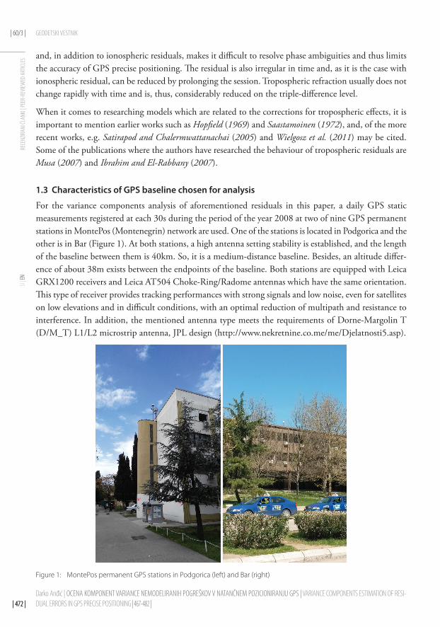
1.3 Characteristics of GPS baseline chosen for analysis
For the variance components analysis of aforementioned residuals in this paper, a daily GPS static measurements registered at each 30s during the period of the year 2008 at two of nine GPS permanent stations in MontePos (Montenegrin) network are used. One of the stations is located in Podgorica and the other is in Bar (Figure 1). At both stations, a high antenna setting stability is established, and the length of the baseline between them is 40km. So, it is a medium-distance baseline. Besides, an altitude differ-ence of about 38m exists between the endpoints of the baseline. Both stations are equipped with Leica GRX1200 receivers and Leica AT504 Choke-Ring/Radome antennas which have the same orientation. This type of receiver provides tracking performances with strong signals and low noise, even for satellites on low elevations and in difficult conditions, with an optimal reduction of multipath and resistance to interference. In addition, the mentioned antenna type meets the requirements of Dorne-Margolin T (D/M_T) L1/L2 microstrip antenna, JPL design (http://www.nekretnine.co.me/me/Djelatnosti5.asp).
Figure 1: MontePos permanent GPS stations in Podgorica (left) and Bar (right)
Darko Anđić | OCENA KOMPONENT VARIANCE NEMODELIRANIH POGREŠKOV V NATANČNEM POZICIONIRANJU GPS | VARIANCE COMPONENTS ESTIMATION OF RESI-DUAL ERRORS IN GPS PRECISE POSITIONING | 467-482 |
| 473 || 473 || 473 |
GEODETSKI VESTNIK | 60/3 |
RECE
NZIRA
NI ČL
ANKI
| PEE
R-RE
VIEW
ED AR
TICLE
SSI
| EN
In post-processing of GPS measurements, MontePos station in Bar was used as the fixed baseline station, so all of the effects for analysis have been contained in the resulting fixed solutions for relative coordi-nates n, e and u which are used as input data for the variance components calculations. The year 2008 was chosen because the same is related to minimal sunspot activities within the respective well-known 11-year period, when there were no increased ionospheric influences which would make it difficult to resolve phase ambiguities in the post-processing.
Trimble Total Control v2.7 software was used herein. Before the post-processing, the following settings in the software were previously done: Processing Interval – 30s; Preference – Prefer P Code; Elevation Cutoff – 10°; Orbit Type – Precise; Frequency – Lc (for baselines longer than 5km); Antenna Model – US NGS ant_info.003; Tropospheric Model – Saastamoinen; Meteorological Model – MSIS; Processing Mode – OTF (as an auxiliary mode for phase ambiguities resolving for each epoch). In addition, in the software Processing Options the Filter for solutions was set to always choose the Best Solution among the solutions obtained from the available linear combinations of the measurements, L0 (Ionosphere-Free), LN (Narrow-Lane) and LW (Wide-Lane).
2 METHODS
In this paper, in addition to the theory based on the two-factor hierarchical classification with ran-dom effects which was presented by Searle (1971) and Hald (1957), the idea of PERG2FH method is used (Perović, 2015), but with some modifications (explanation in footnote 1). Due to the limited scope of this paper, the author briefly presents a linear model which the method is based on, but all of the used formulas have been included. For details, the reader is referred to the monograph (Perović, 2015), where the mathematical apparatus presented by Searle (1971) and Hald (1957) was skillfully and concisely given. The author of the monograph also gave a certain scientific contribu-tion for the case of unbalanced data that occurs in the two-factor hierarchical classification issue. In sense of what has been mentioned before, research in this paper is based on linear two-factor model of hierarchical classification with random effects, with a different number of measurements per groups (Searle, 1971):
= µ +α +β + ε = = =; 1,2,..., , 1,2,..., , 1,2,...,ijk i ij ijk i ijY i a j b k n , (1)
with:
..= = = == = = = = ≥ ≥ ≥∑ ∑ ∑ ∑,1 1 1 1, ; 2, 2, 2.i ib a a b
i ij i i ij ij ij i i jN n n B b b N n n b a (2)
In accordance to discussion in this paper, we have the following notations in (1): Yijk – the fixed solution
for the relative coordinate n, e or u (measurement), µ – a general mean, αi – the combined random effect oftropospheric and ionospheric refraction, βij – the random effect of signal multipath 1 (nested within αi) and
εijk
– the pure random error, or, shortened “pure” error (nested within βij).
In this paper, because of the large number of measurements, it may be considered that µ equals ‘’true value’’ of the measurement Yijk, denoted by AY , which leads to the fact that the constant systematic error (fixed parameter denoted by δ) in the model (1) can be written as δ = µ − AY = 0. Thus, instead of the 1 Perović (2015) has conected this effect to quasi-stationary atmospheric blocks
Darko Anđić | OCENA KOMPONENT VARIANCE NEMODELIRANIH POGREŠKOV V NATANČNEM POZICIONIRANJU GPS | VARIANCE COMPONENTS ESTIMATION OF RESI-DUAL ERRORS IN GPS PRECISE POSITIONING | 467-482 |

| 474 || 474 || 474 |
| 60/3 | GEODETSKI VESTNIK
RECE
NZIRA
NI ČL
ANKI
| PEE
R-RE
VIEW
ED AR
TICLE
SSI
| EN
model (1), the author uses the following linear model of true errors:
∆ = α +β + ε = = =, 1,2,..., , 1,2,..., , 1,2,..., .ijk i ij ijk i iji a j b k n (3)
This linear model is followed by corresponding stochastic model:
α β εα σ β σ ε σ2 2 2~ (0, ), ~ (0, ), ~ (0, ),i ij ijkN N N (4)
cov cov cov cov( , ) ( , ) ( , ) 0, ( , ) 0 ( ),i ij i ijk ij ijk ijk pqr p q k rα β = α ε = β ε = ε ε = ≠ ∨ ≠ ∨ ≠i j (5)
and, in addition:
∆∆ σ = = =2~ (0, ); 1,2,..., , 1,2,..., , 1,2,..., .ijk iji a i a k nN (6)
With respect to (3), (4) and (6), we have:
∆ ∆ α β εσ ≡ σ = σ + σ + σ = = =2 2 2 2 2 ; 1,2,..., , 1,2,..., , 1,2,..., ,ijk i iji a j b k n (7)
where σα2, σβ
2 and σε2 are variance components which the variance σY
2 consists of, and they are determined from the true errors given in (3).
The author divided the set of all true errors for the contemplated year by days and within each established subset, particularly for each of the coordinates (n, e and u), he has carried out the following procedure:
1. Checking of behavior of the true errors using graphical presentations and removing of blunders with the magnitudes of several decimeters which can be easily detected;
2. In order to estimate variance component σε2, previously, all of the subsets of true errors established
by days have to be divided into groups, so that all of those groups correspond to time interval within which we can consider that the factor β causes almost constant effect (following the con-dition in PERG2FH method (Perović, 2015));
3. For estimation of variance component σβ2 it is necessary to divide the set of all true errors into
the groups, so that all of those groups correspond to time interval within which we can consider that, now, the factor α causes almost constant effect (following the condition in PERG2FH method (Perović, 2015));
4. Calculation of values given in (2);5. Calculation of the following independent sums of squares (following Searle (1971), whereby
instead of Y we put ∆ everywhere):
2 2 21 1 1 1 1 1( ) , ( ) , ( ) ,i i ija a b a b n
i i ij ij i ijk iji i j i j kSSA N SSB n SSE= = = = = == ∆ − ∆ = ∆ − ∆ = ∆ ∆∑ ∑ ∑ ∑ ∑ ∑ − (8)
using:
. ... .. == =
∆ ∆∆ = ∆ = ∆ ∆ = ∆ = ∆11 1, ; , ;ij ijin nij bi
ij ij ijk i i ijkjk kij in N
Σ Σ Σ (9)
...... = = =
∆∆ = ≈ ∆ = ∆1 1 10, ;iji nba
i ijkj kNΣ Σ Σ (9’)
6. Calculation of mean squares (Searle, 1971):
Darko Anđić | OCENA KOMPONENT VARIANCE NEMODELIRANIH POGREŠKOV V NATANČNEM POZICIONIRANJU GPS | VARIANCE COMPONENTS ESTIMATION OF RESI-DUAL ERRORS IN GPS PRECISE POSITIONING | 467-482 |
| 475 || 475 || 475 |
GEODETSKI VESTNIK | 60/3 |
RECE
NZIRA
NI ČL
ANKI
| PEE
R-RE
VIEW
ED AR
TICLE
SSI
| EN
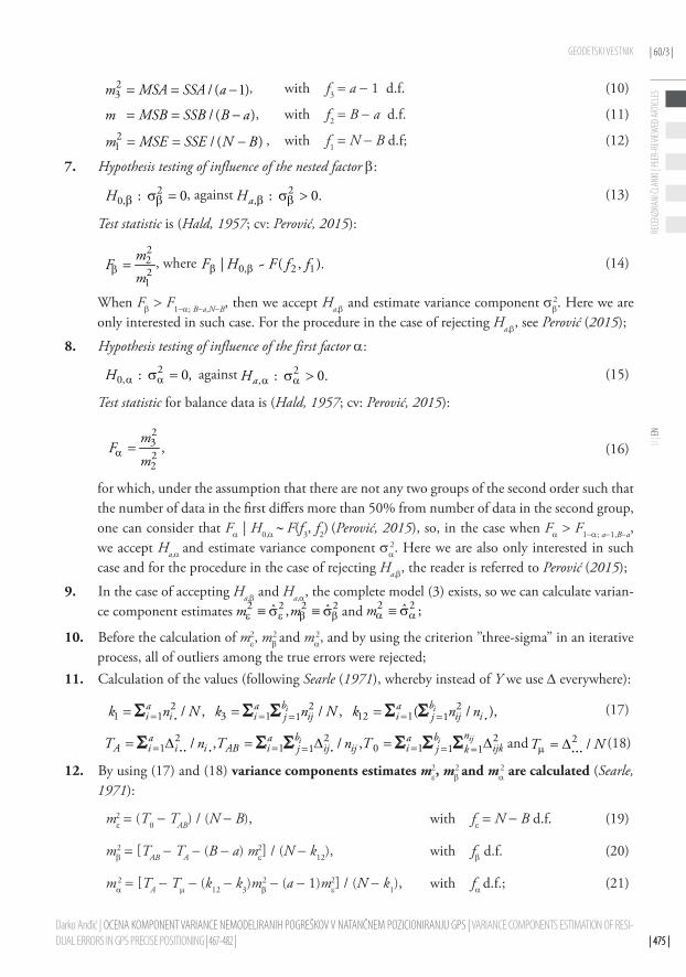
23 / ( 1)m MSA SSA a= = − , with f3 = a − 1 d.f. (10)
/ ( )m MSB SSB B a= = − , with f2 = B − a d.f. (11)
21 / ( )m MSE SSE N B= = − , with f1 = N − B d.f; (12)
7. Hypothesis testing of influence of the nested factor β:
20, : 0H β βσ = , against 2
, : 0.aH β βσ > (13)
Test statistic is (Hald, 1957; cv: Perović, 2015):
2221
mF
mβ = , where 0, 2 1| ~ ( , ).F H F f fβ β (14)
When Fβ > F1−α; B−a,N−B, then we accept Ha,β and estimate variance component σβ2. Here we are
only interested in such case. For the procedure in the case of rejecting Ha,β, see Perović (2015);
8. Hypothesis testing of influence of the first factor α:
20, : 0,H α ασ = against 2
, : 0.aH α ασ > (15)
Test statistic for balance data is (Hald, 1957; cv: Perović, 2015):
2322
,m
Fm
α = (16)
for which, under the assumption that there are not any two groups of the second order such that the number of data in the first differs more than 50% from number of data in the second group, one can consider that Fα | H0,α ∼ F(f3, f2) (Perović, 2015), so, in the case when Fα > F1−α; a−1,B−a, we accept Ha,α and estimate variance component σα
2. Here we are also only interested in such case and for the procedure in the case of rejecting Ha,β, the reader is referred to Perović (2015);
9. In the case of accepting Ha,β and Ha,α, the complete model (3) exists, so we can calculate varian-ce component estimates 2 2 2 2ˆ ˆ,m mε ε β β≡ σ ≡ σ and 2 2ˆ ;mα α≡ σ
10. Before the calculation of mε2, mβ
2 and mα2, and by using the criterion ’’three-sigma’’ in an iterative
process, all of outliers among the true errors were rejected;11. Calculation of the values (following Searle (1971), whereby instead of Y we use ∆ everywhere):
. .= = == == = =2 2 21 1 3 1 12 11 1/ , / , ( / ),i ib ba a a
i i i ij i ij ij jk n N k n N k n nΣ Σ Σ Σ Σ (17)
2 2 21 1 0 11 1 1/ , / , iji i nb ba a a
A i i i AB i ij ij i ijkj j kT n T n T= = == = == ∆ = ∆ = ∆. . . .Σ Σ Σ Σ Σ Σ and 2 /T Nµ = ∆. . . (18)
12. By using (17) and (18) variance components estimates mε2, mβ
2 and mα2 are calculated (Searle,
1971):
mε2 = (T0 − TAB) / (N − B), with fε = N − B d.f. (19)
mβ2 = [TAB − TA − (B − a) mε
2] / (N − k12), with fβ d.f. (20)
mα2 = [TA − Tµ − (k12 − k3)mβ
2 − (a − 1)mε2] / (N − k1), with fα d.f.; (21)
Darko Anđić | OCENA KOMPONENT VARIANCE NEMODELIRANIH POGREŠKOV V NATANČNEM POZICIONIRANJU GPS | VARIANCE COMPONENTS ESTIMATION OF RESI-DUAL ERRORS IN GPS PRECISE POSITIONING | 467-482 |
| 476 || 476 || 476 |
| 60/3 | GEODETSKI VESTNIK
RECE
NZIRA
NI ČL
ANKI
| PEE
R-RE
VIEW
ED AR
TICLE
SSI
| EN
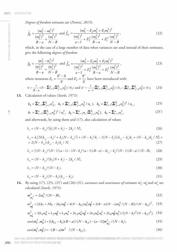
Degrees of freedom estimates are (Perović, 2015):
2 2 22 1
2 2 2 22 1
( )ˆ( ) ( )
m mf
m mB a N B
β−
=+
− −
and 2 2 2 23 2 2 1 1
2 2 2 2 2 22 23 2 12 1
( )ˆ ,( ) ( ) ( )
1
m E m E mf
m m mE E
a B a N B
α− +
=
+ +− − −
(22)
which, in the case of a large number of data when variances are used instead of their estimates, give the following degrees of freedom:
2 2 22
2 22 22
( )( )( )
f
B a N B
εβ
ε
σ −σ=
σσ+
− −
and 2 2 2 23 2 2 1 1
2 2 2 2 2 22 23 2 12 1
( )ˆ ,( ) ( ) ( )
1
m E m E mf
m m mE E
a B a N B
α− +
=
+ +− − −
(23)
where notations 1n n
En′ −
= and 2n
En′
= have been introduced with:
21 1
1( ( ) / )iba
i ij ijn N n NB a = == −−
Σ Σ and
= 2 21 11 1
1( ( ) / ( ) / );
1i ib ba a
i ij i i ijj jn n N n Na = == =′ −−Σ Σ Σ Σ (24)
13. Calculation of values (Searle, 1971):
. .= = == = == = =3 3 2 24 1 5 1 6 11 1 1, ( / ), ( ) / ,i i ib b ba a a
i ij i ij i i ij ij j jk n k n n k n nΣ Σ Σ Σ Σ Σ (25)
. . .= = == == = =2 2 2 2 37 1 8 1 9 11 1( ) / , ( ), ,i ib ba a a
i ij i i i ij i ij jk n n k n n k nΣ Σ Σ Σ Σ (25’)
and afterwards, by using them and (17), also calculation of values:
λ1 = (N − k12)2[k1(N + k1) − 2k9 / N], (26)
λ2 = k3[N(k12 − k3)2 + k3(N − k12)
2] + (N − k3)2k7 − 2(N − k3)[(k12 − k3)k5 + (N − k12)k6 / N] +
+ 2(N − k12)(k12 − k3)k4 / N, (27)
λ3 = [(N − k12)2(N − 1)(a − 1) − (N − k3)
2(a − 1)(B − a) − (k12 − k3)2(N − 1)(B − a) / (N − B), (28)
λ4 = (N − k12)2[k3(N + k1) − 2k8 / N], (29)
λ5 = (N − k12)2(N − k1), (30)
λ6 = (N − k12)(N − k3)(k12 − k3); (31)
14. By using (17), (25), (25’) and (26)-(31), variances and covariances of estimates mε2, mβ
2 and mα2 are
calculated (Searle, 1971):
22 42 / ( ),m N Bε
ε= −m
m (32)
22 4 2 2 4 2
7 3 5 12 12[2( 2 ) 4( ) 2( )( ) / ( )] / ( ) ,k Nk k m N k m m B a N a m N B N kβ
β ε β ε= + − + − + − − − −m
m (33)
22 4 4 4 2 2 2 2 2 2 2 2
1 2 3 4 5 6 1 122( 2 2 2 ) /[( ) ( ) ],m m m m m m m m m N k N kα
α β ε α β α ε β ε= λ + λ + λ + λ + λ + λ − −m
m (34)
22 2 2
12 3 12 1cov( , ) [( )( ) / ( ) ( 1)] / ( ),k k B a N k a N kε
ε α = − − − − − −mm m m (35)
2 2 212cov( , ) ( ) / ( ),B a N kε β = − − −m m m (36)
Darko Anđić | OCENA KOMPONENT VARIANCE NEMODELIRANIH POGREŠKOV V NATANČNEM POZICIONIRANJU GPS | VARIANCE COMPONENTS ESTIMATION OF RESI-DUAL ERRORS IN GPS PRECISE POSITIONING | 467-482 |
| 477 || 477 || 477 |
GEODETSKI VESTNIK | 60/3 |
RECE
NZIRA
NI ČL
ANKI
| PEE
R-RE
VIEW
ED AR
TICLE
SSI
| EN
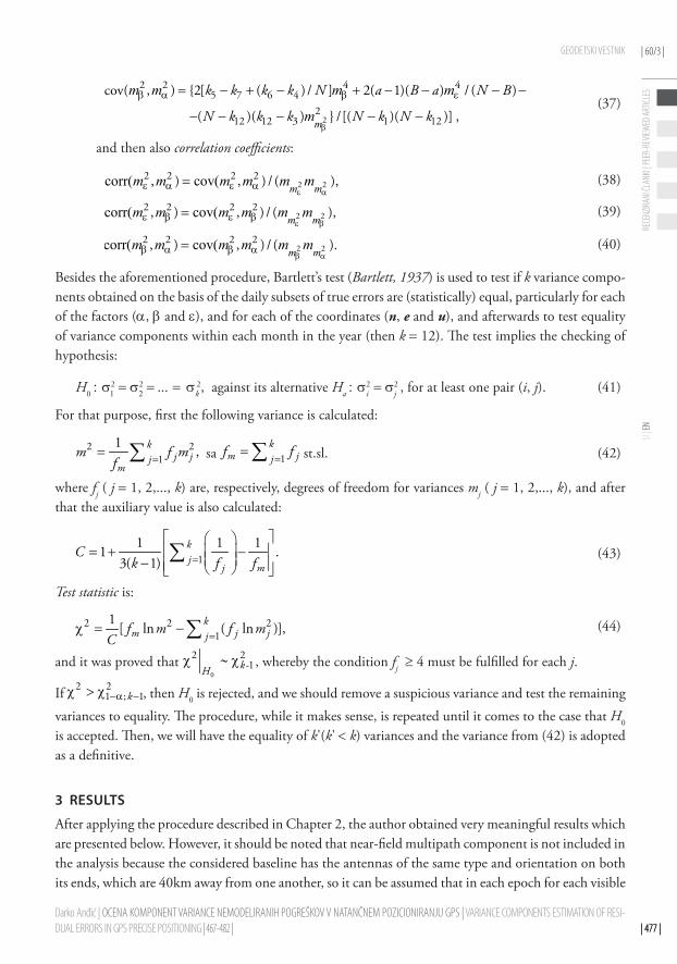
2
2 2 4 45 7 6 4
212 12 3 1
21
22
cov( , ) {2[ ( ) / ] 2( 1)( ) / ( )
( )( ) } /cov( [( )( ,) )],
k k k k N a B a N B
N k k k N k N kβ
β α β ε
β α
= − + − + − − − −
− − − − −= mm m
m m m m
m (37)
and then also correlation coefficients:
corr( cov( 2 22 2 2 2, ) , ) / ( ),
ε αε α ε α= m mm m m m m m (38)
corr( cov( 2 22 2 2 2, ) , ) / ( ),
ε βε β ε β= m mm m m m m m (39)
corr( cov( 2 22 2 2 2, ) , ) / ( ).
β αβ α β α= m mm m m m m m (40)
Besides the aforementioned procedure, Bartlett’s test (Bartlett, 1937) is used to test if k variance compo-nents obtained on the basis of the daily subsets of true errors are (statistically) equal, particularly for each of the factors (α, β and ε), and for each of the coordinates (n, e and u), and afterwards to test equality of variance components within each month in the year (then k = 12). The test implies the checking of hypothesis:
H0 : σ12 = σ2
2 = ... = σk2, against its alternative Ha : σi
2 = σj2 , for at least one pair (i, j). (41)
For that purpose, first the following variance is calculated:
2 21
1,k
j jjm
m f mf == ∑ sa
1k
m jjf f== ∑ st.sl. (42)
where fj ( j = 1, 2,..., k) are, respectively, degrees of freedom for variances mj ( j = 1, 2,..., k), and after that the auxiliary value is also calculated:
1
1 1 11 .
3( 1)kj
j mC
k f f=
= + − − ∑ (43)
Test statistic is:
2 2 21
1[ ln ( ln )],k
m j jjf m f mC =χ = −∑ (44)
and it was proved that 0
2 2-1kH
χ ∼ χ , whereby the condition fj ≥ 4 must be fulfilled for each j.
If 2 21 ; 1k−α −χ > χ , then H0 is rejected, and we should remove a suspicious variance and test the remaining
variances to equality. The procedure, while it makes sense, is repeated until it comes to the case that H0 is accepted. Then, we will have the equality of k'(k' < k) variances and the variance from (42) is adopted as a definitive.
3 RESULTS
After applying the procedure described in Chapter 2, the author obtained very meaningful results which are presented below. However, it should be noted that near-field multipath component is not included in the analysis because the considered baseline has the antennas of the same type and orientation on both its ends, which are 40km away from one another, so it can be assumed that in each epoch for each visible
Darko Anđić | OCENA KOMPONENT VARIANCE NEMODELIRANIH POGREŠKOV V NATANČNEM POZICIONIRANJU GPS | VARIANCE COMPONENTS ESTIMATION OF RESI-DUAL ERRORS IN GPS PRECISE POSITIONING | 467-482 |
| 478 || 478 || 478 |
| 60/3 | GEODETSKI VESTNIK
RECE
NZIRA
NI ČL
ANKI
| PEE
R-RE
VIEW
ED AR
TICLE
SSI
| EN
satellite the values of elevation angle and azimuth was identical at both ends of the baseline, because of which the impact of near-field component was always completely cancelled out in double-difference phase observations.
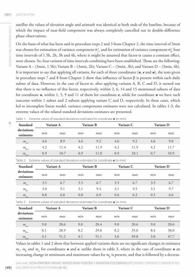
On the basis of what has been said in procedure steps 2 and 3 from Chapter 2, the time interval of 3min was chosen for estimation of variance component σε
2, and for estimation of variance component σβ2 four
time intervals of 1.5h, 2h, 3h and 4h, where it might be assumed that factor α causes a constant effect, were chosen. So, four variants of time intervals combining have been established. Those are the following: Variant A – (3min, 1.5h); Variant B – (3min, 2h); Variant C – (3min, 3h); and Variant D – (3min, 4h). It is important to say that applying all variants, for each of three coordinates (n, e and u), the tests given in procedure steps 7 and 8 from Chapter 2 show that influence of factor β is present within each daily subset of data. However, in the case of factor α, after applying variants A, B, C and D, it turned out that there is no influence of this factor, respectively, within 2, 6, 14 and 15 mentioned subsets of data for coordinate n, within 1, 5, 9 and 11 of them for coordinate e, while for coordinate u we have such outcome within 1 subset and 2 subsets applying variant C and D, respectively. In these cases, which led to incomplete linear model, variance components estimates were not calculated. In tables 1-3, the extreme values of the related standard deviations estimates are presented.
Table 1: Extreme values of standard deviations estimates for coordinate n (in mm)
Standard deviations estimates
Variant A Variant B Variant C Variant D
min max min max min max min max
mε;n 4.6 8.9 4.6 9.2 4.6 9.2 4.6 9.0
mβ;n 4.2 11.4 4.2 11.9 4.2 11.9 4.2 11.7
mα;n 0.9 10.7 0.9 11.0 0.9 10.1 0.7 10.9
Table 2: Extreme values of standard deviations estimates for coordinate e (in mm)
Standard deviations estimates
Variant A Variant B Variant C Variant D
min max min max min max min max
mε;e 3.5 6.7 3.5 6.7 3.5 6.7 3.5 6.7
mβ;e 3.0 9.1 3.1 9.4 3.1 9.5 3.1 9.7
mα;e 0.8 6.8 0.8 6.9 0.6 6.2 0.5 6.6
Table 3: Extreme values of standard deviations estimates for coordinate u (in mm)
Standard deviations estimates
Variant A Variant B Variant C Variant D
min max min max min max min max
mε;u 9.0 20.6 9.0 20.4 9.0 20.6 9.0 20.6
mβ;u 8.1 28.9 8.2 29.8 8.2 35.0 8.4 38.0
mα;u 4.1 51.2 4.1 51.1 3.6 49.8 3.0 47.7
Values in tables 1 and 2 show that between applied variants there are no significant changes in estimates mε, mβ and mα for coordinates n and e, unlike those in table 3, where in the case of coordinate u an increasing change in minimum and maximum values for mβ is present, and that is followed by a decreas-
Darko Anđić | OCENA KOMPONENT VARIANCE NEMODELIRANIH POGREŠKOV V NATANČNEM POZICIONIRANJU GPS | VARIANCE COMPONENTS ESTIMATION OF RESI-DUAL ERRORS IN GPS PRECISE POSITIONING | 467-482 |

| 479 || 479 || 479 |
GEODETSKI VESTNIK | 60/3 |
RECE
NZIRA
NI ČL
ANKI
| PEE
R-RE
VIEW
ED AR
TICLE
SSI
| EN
ing change in minimum and maximum values for mα. This leads to the conclusion that by expanding time intervals in variants C and D we have partial mixing, i.e. ‘’overflowing’’ of the effect of factor α in estimate mβ. On the other side, if comparing variants A and B, there are no significant changes in mβ and mα values for any of three coordinates (n, e and u), while mε values are, as expected, practically equal between variants.
Based on the foregoing, and considering that, according to the previous research, the maximum period for far-field multipath component is 30min, as a reasonable choice among applied variants, the variant B is adopted. Therefore, only the results of the analysis obtained by applying this variant are presented hereinafter.
So, in Figure 2, graphical presentations of standard deviations estimates obtained by applying variant B, are presented.
Figure 2: Behaviour of standard deviations estimates (in mm) (blue - mε, green - mβ, red - mα)
In Table 4, extreme absolute values of correlation coefficients of obtained variance components estimates are presented. They show very low correlations, therefore, practically, there is no correlation. Such a case testifies to the fact that adequate variance components estimation method was used.Table 4: Extreme absolute values of correlation coefficients of variance components estimates (in %)
Absolute values of
correlation coefficients
Coordinaten
Coordinatee
Coordinateu
min max min max min max
| corr(mε2, mβ
2) | 2.6 11.8 2.1 11.2 1.3 10.3
| corr(mε2, mα
2) | 0.0 0.0 0.0 0.0 0.0 0.0
| corr(mβ2, mα
2) | 0.3 7.6 0.3 7.5 0.1 3.3
Applying Bartlett’s test, the equality of all variance components estimates was tested and it has turned out that for any factor (ε, β and α) and any coordinate (n, e and u), there is no equality. On the other side, the same test was applied within each month for all the factors and coordinates. Because of the limited scope of this paper, all results of testing are not presented herein. However, it is of an impor-
Darko Anđić | OCENA KOMPONENT VARIANCE NEMODELIRANIH POGREŠKOV V NATANČNEM POZICIONIRANJU GPS | VARIANCE COMPONENTS ESTIMATION OF RESI-DUAL ERRORS IN GPS PRECISE POSITIONING | 467-482 |

| 480 || 480 || 480 |
| 60/3 | GEODETSKI VESTNIK
RECE
NZIRA
NI ČL
ANKI
| PEE
R-RE
VIEW
ED AR
TICLE
SSI
| EN
tance to note that, for the adopted significance level of 0.05, and after applying an iterative procedure of Bartlett’s test, it turned out that for coordinates n, e and u we have equality of the variance compo-nents estimates within each month, but only in the case of the factor α, with the mean percentage of removed variances of 11%, 8% and 35%, respectively. The unified variance components estimates for each month are presented in Table 5. Because of large number of data they were obtained from, we can say they represent variance components.
Table 5: Unified variance components estimates (in mm2) and their degrees of freedom estimates for factor α
MonthCoordinate
nCoordinate
eCoordinate
u
mα2 fˆm; α mα
2 fˆm; α mα2 fˆm; α
January 5.0531 196.5 3.1007 187.6 113.9751 198.7
February 7.3022 172.2 4.7019 170.8 88.7458 109.7
March 10.2702 174.6 5.8493 143.2 179.8221 125.8
April 9.3085 201.6 7.0534 192.8 304.9260 247.2
May 8.1065 156.4 5.9720 210.5 151.9056 135.4
June 42.7210 219.4 15.2606 193.9 314.8144 133.6
July 28.9726 214.0 14.0820 195.7 408.9308 189.4
August 34.0538 255.1 13.8782 220.3 370.0660 160.6
September 11.9485 181.3 8.8691 188.7 264.0705 227.1
October 9.3549 206.7 7.8849 254.5 248.5245 203.8
November 7.1575 173.2 5.2894 206.3 108.4320 141.8
December 8.0308 186.1 5.5280 192.9 94.4073 190.6
Values in Table 5 show that the monthly standard deviations estimates of residuals arising due to combined tropospheric and ionospheric effects, for GPS baseline Podgorica-Bar (of 40km in length), and during the year 2008 with a minimal sunspot activity, are, for the coordinates n, e and u, in the intervals ~2.2-6.5mm, ~1.8-3.9mm and ~9.4-20.2mm, respectively. By checking of equality of 12 unified variances in the same table, it turned out that for any coordinate (n, e and u) there is no equality.
On the other side, for factors ε and β, and for the same significance level, we have no equality of variance components estimates, so they were not unified within months.
4 DISCUSSIONThe research in this paper has shown that by using the two-way nested classification linear model one can integrally estimate the variance components of residual and pure random errors arising in GPS precise positioning, which is of a great importance, because a big step for the GPS data analysis has been made.
On the basis of the results obtained through the analysis, it is obvious that the highest variations of multipath and combined tropospheric and ionospheric residuals are present in summer period of the year and the lowest ones in winter period, which is in accordance with the year sunspot activities.
Each GPS site has its environmental characteristics and thus, especially, a specific periods of multipath errors. A frequences of those periods are not the issue of this paper. However, the estimation of those
Darko Anđić | OCENA KOMPONENT VARIANCE NEMODELIRANIH POGREŠKOV V NATANČNEM POZICIONIRANJU GPS | VARIANCE COMPONENTS ESTIMATION OF RESI-DUAL ERRORS IN GPS PRECISE POSITIONING | 467-482 |
| 481 || 481 || 481 |
GEODETSKI VESTNIK | 60/3 |
RECE
NZIRA
NI ČL
ANKI
| PEE
R-RE
VIEW
ED AR
TICLE
SSI
| EN
frequencies might be the issue for a further research. In the basis of such a research, the application of the nonlinear least-squares method would be relevant in searching for the related periodicity of GPS residual data, whose behaviour can be presented by trigonometric functions involving a multiple perio-dicity (two or more frequencies).
In addition, a further research might be also based on the application of a particular linear combination of GPS observations in the calculations of fixed solutions, where the impact of that on the magnitudes of variance components of residual errors could be analysed. The problem should also be considered depending on the GPS baseline length and/or its azimuth.
Literature and references:Asgari, J., Amiri-Simkooei, A. R. (2011). Analysis and Prediction of GNSS Estimated
Total Electron Contents. Journal of the Earth & Space Physics, 37 (1), 11–24.
Bartlett, M. S. (1937). Properties of Sufficiency and Statistical Tests. Proceedings of the Royal Society of London. Series A 160, 268–282.
DOI: http://dx.doi.org/10.1098/rspa.1937.0109
Beutler, G., Bauersima, I., Gurtner, W., Rothacher, M., Schildknecht, T., Geiger, A. (1988). Atmospheric refraction and other important biases in GPS carrier phase observations. In: Atmospheric Effects on Geodetic Space Measurements. Monograph 12, pp.15–43. Kensington: School of Surveying. University of New South Wales.
El-Hattab, A. I. (2013). Influence of GPS antenna phase center variation on precise positioning. NRIAG Journal of Astronomy and Geophysics, 2 (2), 272–277. DOI: http://dx.doi.org/10.1016/j.nrjag.2013.11.002
Elósegui, P., Davis, J. L., Jaldehag, R. T. K., Johansson, J. M., Niell, A. E., Shapiro, I. I. (1995). Geodesy using the Global Positioning System: The effects of signal scattering on estimates of site position. Journal of Geophysical Research, 100 (B6), 9921–9934. DOI: http://dx.doi.org/10.1029/95JB00868
Fan, K. K., Ding, X. L. (2006). Estimation of GPS Carrier Phase Multipath Signals Based on Site Environment. Journal of Global Positioning Systems, 5 (1–2), 22–28. DOI: http://dx.doi.org/10.5081/jgps.5.1.22
Fritsche, M., Dietrich, R., Knöfel, C., Rülke, A., Vey, S., Rothacher, M. and Steigenberger, P. (2005). Impact of higher-order ionospheric terms on GPS estimates, Geophysical Research Letters, 32 (L23311), 1–5.
DOI: http://dx.doi.org/10.1029/2005GL024342
Hald, A. (1957). Statistical Theory with Engineering Applications (3rd printing). New York: John Wiley & Sons, Inc. London: Chapman & Hall, Ltd.
Hopfield, H. S. (1969). Two-quartic tropospheric refractivity profile for correcting satellite data. Journal of Geophysical Research, 74 (8), 4487–4499.
DOI: http://dx.doi.org/10.1029/jc074i018p04487
Hoque, M. M., Jakowski, N. (2008). Estimate of higher order ionospheric errors in GNSS positioning. Radio Science, 43 (RS5008), 1–15.
DOI: http://dx.doi.org/10.1029/2007RS003817
Ibrahim, H. E., El-Rabbany, A. (2007). Stochastic Modeling of Residual Tropospheric Delay. Proceedings of the 2007 National Technical Meeting of The Institute of Navigation. San Diego, CA, January 2007, pp.1044–1049.
Kouba, J. (2009). A guide to using International GNSS Service (IGS) products. http://igscb.jpl.nasa.gov/igscb/resource/pubs/UsingIGSProductsVer21.pdf, accessed 5. 11. 2010.
Leick, A. (2004). GPS Satellite Surveying (3rd Edition). Hoboken-New Jersey: John Wiley & Sons, Inc.
Leick, A., Rapoport, L., Tatarnikov, D. (2015). GPS Satellite Surveying. 4th Edition. Hoboken-New Jersey: John Wiley & Sons, Inc.
Miller, S., Zhang, X., Spanias, A. (2015). Multipath Effects in GPS Receivers. A Publication in the Morgan & Claypool Publishers series Synthesis lectures on communications. William Tranter, Virginia Tech (ed). Morgan & Claypool 2016.
Musa, T. A. (2007). Analysis of Residual Atmospheric Delay in the Low Latitude Regions Using Network-Based GPS Positioning. PhD Thesis. Sydney: School of Surveying and Spatial Information Systems, The University of New South Wales.
Perović, G. (2015). Theory of measurement errors (in Serbian: Teorija grešaka merenja). Belgrade: AGM knjiga.
Saastamonien, J. (1972). Contribution to the theory of atmospheric refraction. Bulletin Géodésique, 105 (1), 279–298. DOI: http://dx.doi.org/10.1007/bf02521844
Santerre, R. (1989). GPS satellite sky distribution: Impact on the propagation of some important errors in precise relative positioning. PhD thesis. Technical Report, No.145. New Brunswick: Department of Surveying Engineering, University of New Brunswick.
Satirapod, C., Chalermwattanachai, P. (2005). Impact of Different Tropospheric Models on GPS Baseline Accuracy: Case Study in Thailand. Journal of Global Positioning Systems, 4 (1–2), 36–40. DOI: http://dx.doi.org/10.5081/jgps.4.1.36
Searle, S. (1971). Linear Models. New York-Chichester-Weinheim-Brisbane-Singapore-Toronto: John Wiley & Sons, Inc.
Seeber, G. (2003). Satellite Geodesy. 2nd completely revised and extended edition. Berlin: Walter de Gruyter GmbH & Co. KG.
DOI: http://dx.doi.org/10.1515/9783110200089
Steigenberger, P. (2009). Reprocessing of a global GPS network. Deutsche Geodätische Kommission, No. C640. Munich: Verlag der Bayerischen Akademie der Wissenschaften.
Wielgosz, P., Cellmer, S., Rzepecka, Z., Paziewski, J., Grejner-Brzezinska, D. A. (2011). Troposphere modeling for precise GPS rapid static positioning in mountainous areas. Measurement Science and Technology, 22 (4), 89–99.
DOI: http://dx.doi.org/10.1088/0957-0233/22/4/045101
Darko Anđić | OCENA KOMPONENT VARIANCE NEMODELIRANIH POGREŠKOV V NATANČNEM POZICIONIRANJU GPS | VARIANCE COMPONENTS ESTIMATION OF RESI-DUAL ERRORS IN GPS PRECISE POSITIONING | 467-482 |

| 482 || 482 || 482 |
| 60/3 | GEODETSKI VESTNIK
RECE
NZIRA
NI ČL
ANKI
| PEE
R-RE
VIEW
ED AR
TICLE
SSI
| EN
Darko Anđić, M.Sc.Real Estate Administration of Montenegro
Ul. Bracana Bracanovića b.bPodgorica, Montenegro
E-mail: [email protected]
Anđić D. (2016). Variance components estimation of residual errors in GPS precise positioning. Geodetski vestnik, 60 (3): 467-482. DOI: 10.15292/geodetski-vestnik.2016.03.467-482
Wildt, S. (2006). Mehrwegeausbreitung bei GNSS-gestützter Positionsbestimmung. PhD thesis. Dresden: Fakultät für Forst-, Geo- und Hydrowissenschaften der TU Dresden.
Wübbena, G., Schmitz, M. and Boettcher, G. (2006). Near-field Effects on GNSS Sites: Analysis using Absolute Robot Calibrations and Procedures to Determine Corrections. Submitted to Proceedings of the IGS Workshop 2006 Perspectives and Visions for 2010 and beyond, May 8-12. ESOC, Darmstadt, Germany.
Darko Anđić | OCENA KOMPONENT VARIANCE NEMODELIRANIH POGREŠKOV V NATANČNEM POZICIONIRANJU GPS | VARIANCE COMPONENTS ESTIMATION OF RESI-DUAL ERRORS IN GPS PRECISE POSITIONING | 467-482 |