Development of Finite Element-based Models for Defect

University of Calgary

PRISM: University of Calgary's Digital Repository

Graduate Studies The Vault: Electronic Theses and Dissertations

2020-07-16

Development of Finite Element-based Models for

Defect Assessment on Pipelines

Sun, Jialin

Sun, J. (2020). Development of Finite Element-based Models for Defect Assessment on Pipelines

(Unpublished doctoral thesis). University of Calgary, Calgary, AB.

http://hdl.handle.net/1880/112305

doctoral thesis

University of Calgary graduate students retain copyright ownership and moral rights for their

thesis. You may use this material in any way that is permitted by the Copyright Act or through

licensing that has been assigned to the document. For uses that are not allowable under

copyright legislation or licensing, you are required to seek permission.

Downloaded from PRISM: https://prism.ucalgary.ca

UNIVERSITY OF CALGARY

Development of Finite Element-based Models for Defect Assessment on Pipelines

by

Jialin Sun

A THESIS

SUBMITTED TO THE FACULTY OF GRADUATE STUDIES

IN PARTIAL FULFILMENT OF THE REQUIREMENTS FOR THE

DEGREE OF DOCTOR OF PHILOSOPHY

GRADUATE PROGRAM IN MECHANICAL AND MANUFACTURING ENGINEERING

CALGARY, ALBERTA

JULY, 2020

© Jialin Sun 2020

ii

Abstract

Pipelines have been the most effective and efficient method for transportation of oil and

gas from production sites to their markets and end users. Assessment of corrosion defects and their

effect on pipeline integrity are critical to the safe operation of pipeline systems. Although

numerous efforts have been made on defect assessment, there are still significant rooms for

research and development in assessment of the interaction of multiple features on pipelines.

In this work, finite element (FE) based models were developed to assess API X46, X60

and X80 steel pipelines containing multiple corrosion defects, which were either longitudinally

aligned, circumferentially aligned or overlapped with each other. The defect size and the grade of

pipeline steels were considered to evaluate the interaction between adjacent defects. The critical

spacing between the defects with various orientations was determined, enabling assessment

whether an interaction existed to affect the failure pressure of the pipeline.

FE models enabling predictions of the failure pressure of pipelines containing a dent

associated with a corrosion defect were also developed. In addition, a failure pressure-based

criterion to properly assess the interaction of the dent and its adjacent corrosion feature was

established.

The mutual interaction between the adjacent corrosion defects affects not only the local

stress and distribution, but also the electrochemical corrosion rate, due to the so-called mechano-

electrochemical (M-E) effect. Due to the existence of the M-E effect, a new criterion is proposed

to determine whether the mutual interaction exists between the adjacent corrosion defects, i.e., on

the ratio of the anodic current density at the defect adjacency to that of the non-corrosion region

on the pipe body.

iii

Acknowledgements

My deep gratitude goes first to my supervisor, Professor Frank Cheng, who expertly guided

me through my PhD program. His unwavering enthusiasm for science and engineering kept me

constantly engaged with my research.

My appreciation also extends to my laboratory colleagues, Ke Yin, Drs. Yao Yang, Shan

Qian, Qiang Li, and those whose names cannot all be listed here, for their help and support in this

work.

Thanks also go to my friends for helping me survive all the stress these past three years

and Covid-19. Especially, I appreciate Mr. Chad Ford, who has inspired, helped and challenged

me to become a better version of myself. Also, Dr. Ken Fox’s mentoring and encouragement has

been tremendously valuable.

Above ground, I am forever grateful, indebted to my family. Words cannot express my

respect and love for them. They are my superheroes. Finally, I want to thank myself for devoting

almost all the 5 a.m. mornings into this PhD research work.

iv

Dedication

To my beloved mother and grandparents,

who constantly pushed me to study harder when I was a child

v

Table of Contents

Abstract ............................................................................................................................... ii Acknowledgements ............................................................................................................ iii

Dedication .......................................................................................................................... iv Table of Contents .................................................................................................................v List of Tables ................................................................................................................... viii List of Figures and Illustrations ......................................................................................... ix List of Symbols, Abbreviations and Nomenclature ...........................................................xv

CHAPTER ONE: INTRODUCTION ..................................................................................1

1.1 Research background .................................................................................................1 1.2 Research objectives ....................................................................................................3

1.3 Content of thesis ........................................................................................................3

CHAPTER TWO: LITERATURE REVIEW ......................................................................6 2.1 Overview of pipeline corrosion .................................................................................6 2.2 Single corrosion defect ..............................................................................................8

2.2.1 Industry Standards for failure pressure predictions of pipelines containing a single

corrosion defect ..................................................................................................8

2.2.2 Failure pressure prediction by finite element modeling ..................................13 2.2.3 M-E effect ........................................................................................................14 2.2.4 Other studies ....................................................................................................15

2.3 Multiple corrosion defect .........................................................................................16

2.3.1 Overview of multiple corrosion defects ..........................................................16 2.3.2 Interaction rules ...............................................................................................17 2.3.3 Failure pressure prediction for multiple corrosion defects ..............................19

2.3.4 M-E effect ........................................................................................................20 2.4 Dent of pipeline .......................................................................................................20

2.4.1 Plain dents .......................................................................................................21

2.4.2 Dents containing other stress risers .................................................................22 2.4.3 Dents interacting with the adjacent stress risers ..............................................22

CHAPTER THREE: RESEARCH METHODOLOGY ....................................................24 3.1 FE models for failure pressure prediction of pipelines containing multiple corrosion

defects ....................................................................................................................24

3.1.1 Initial and boundary conditions .......................................................................24 3.1.2 Properties of pipeline steels and the failure criterion of pipelines ..................26

3.1.3 Validation of FE modeling results ...................................................................27 3.1.4 FE modeling of longitudinally and circumferentially aligned, as well as

overlapped corrosion defects ...........................................................................30 3.2 FE models for simulation and prediction of the M-E effect at multiple corrosion

defects ....................................................................................................................32

3.2.1 Initial and boundary conditions .......................................................................32 3.2.2 Properties of pipeline steels and electrochemical corrosion parameters .........36

vi

3.2.3 Effect of stress on electrode potential .............................................................39 3.2.4 Comparison of 3D modeling results with the theoretical calculations ............40

3.3 FE models for failure pressure prediction of pipelines containing a corrosion defect

associated with a dent ............................................................................................41

3.3.1 Initial and boundary conditions .......................................................................41 3.3.2 Properties of pipeline steels .............................................................................45 3.3.3 Mesh density analysis ......................................................................................45

CHAPTER FOUR: MODELING OF THE INTERACTION OF MULTIPLE CORROSION

DEFECTS AND ITS EFFECT ON FAILURE PRESSURE OF PIPELINES .........47

4.1 Interaction of longitudinally and circumferentially aligned corrosion defects on

pipelines .................................................................................................................47 4.2 Interaction of overlapped corrosion defects on pipelines ........................................51

4.3 Quantification of interaction of multiple corrosion defects on pipelines ................60

4.4 Summary ..................................................................................................................61

CHAPTER FIVE: MODELING OF MECHANO-ELECTROCHEMICAL INTERACTION

OF MULTIPLE LONGITUDINALLY ALIGNED CORROSION DEFECTS ON

OIL/GAS PIPELINES ..............................................................................................63 5.1 2-D modeling of the M-E effect between corrosion defects on pipelines under axial

stress in NS4 solution.............................................................................................63 5.2 3-D modeling of the M-E effect between corrosion defects on pressurized pipelines in

NS4 solution...........................................................................................................67

5.3 Effect of defect length on M-E effect of corrosion defects .....................................75

5.4 Maximum spacing between corrosion defects for their mutual interaction .............78 5.5 M-E effect of adjacent corrosion defects on pipelines ............................................81 5.6 Summary ..................................................................................................................83

CHAPTER SIX: INVESTIGATION BY NUMERICAL MODELING OF THE MECHANO-

ELECTROCHEMICAL INTERACTION OF CIRCUMFERENTIALLY ALIGNED

CORROSION DEFECTS ON PIPELINES ..............................................................84

6.1 Modeling of stress distribution at circumferentially aligned corrosion defects on

pipelines .................................................................................................................84 6.2 Modeling of corrosion potential at circumferentially aligned corrosion defects on

pipelines .................................................................................................................88 6.3 Modeling of anodic current density at circumferentially aligned corrosion defects on

pipelines .................................................................................................................92 6.4 Analysis of stress, corrosion potential and anodic current density at circumferentially

aligned corrosion defects on pipelines ...................................................................96 6.5 Maximum circumferential spacing of corrosion defects enabling mutual interaction99 6.6 Summary ................................................................................................................104

CHAPTER SEVEN: MODELING OF THE MECHANO-ELECTROCHEMICAL

INTERACTION BETWEEN ADJACENT CIRCUMFERENTIAL CORROSION

DEFECTS ON PIPELINES UNDER AXIAL TENSILE STRESSES...................106 7.1 Modelling of stress distribution at circumferentially aligned corrosion defects ...106

vii

7.2 Modelling of corrosion potential at circumferentially aligned corrosion defects ..110 7.3 Modelling of anodic current density at circumferentially aligned corrosion defects114 7.4 Distributions of von Mises stress, corrosion potential and anodic current density across

the corrosion defects under varied axial tensile stresses ......................................117

7.5 Maximum circumferential spacing enabling interaction between corrosion defects on

pipelines ...............................................................................................................119 7.6 Summary ................................................................................................................124

CHAPTER EIGHT: MODELING OF MECHANO-ELECTROCHEMICAL

INTERACTION AT OVERLAPPED CORROSION DEFECTS AND THE

IMPLICATION ON PIPELINE FAILURE PREDICTION ...................................126

8.1 Modelling of stress and anodic current density at the overlapped corrosion defects

under varied internal pressures ............................................................................126

8.2 Modelling of stress and anodic current density distributions at the overlapped corrosion

defects with varied lengths of the top layer defect ..............................................130 8.3 Modelling of stress and anodic current density distributions at the overlapped corrosion

defects with varied lengths of the bottom layer defect ........................................134

8.4 Modelling of stress and anodic current density distributions at the overlapped corrosion

defects with varied defect depths .........................................................................138

8.5 Effect of defect length on M-E effect at the overlapped corrosion defects ...........143 8.6 Implications on pipeline integrity in the presence of overlapped corrosion defects146 8.7 Summary ................................................................................................................147

CHAPTER NINE: ASSESSMENT OF A DENT INTERACTING WITH CORROSION

FEATURE ON PIPELINES BY FINITE ELEMENT MODELING .....................149 9.1 Quantification of interaction of multiple corrosion defects on pipelines ..............149 9.2 Effect of dent-corrosion feature spacing on pipeline failure .................................151

9.3 Dent-corrosion feature interaction identification rule ...........................................152 9.4 Effect of corrosion depth .......................................................................................154

9.5 Effect of corrosion length ......................................................................................155

9.6 Effect of dent depth ................................................................................................157 9.7 Summary ................................................................................................................158

CHAPTER TEN: CONCLUSIONS AND RECOMMENDATIONS .............................159 10.1 Conclusions ..........................................................................................................159 10.2 Recommendations ................................................................................................162

RESEARCH PUBLICATIONS IN PEER-REVIEWED JOURNALS ...........................163

REFERENCES ................................................................................................................164

viii

List of Tables

Table 3.1. Properties and relevant parameters of three grades of pipeline steel. .......................... 27

Table 3.2. Geometry of corrosion defects present on pipelines published in Benjiamin’s work

[125] ...................................................................................................................................... 28

Table 3.3. Failure pressures of X80 steel pipeline containing different types of corrosion

defects, which are schematically shown in Table 3.2, determined by FE modeling in this

work (PFEM), as a comparison with the testing results (PE) [68]. ......................................... 29

Table 3.4. The initial electrochemical parameters for FE simulation derived from [20] ............. 38

Table 3.5. First principal stress (MPa) and anodic current density (μA/cm2) of X46 steel pipe

in a near neutral solution under various internal pressure determined by FE modeling in

this work, as a comparison with the theoretical calculations. ............................................... 41

Table 4.1. Failure pressures (MPa) of pipelines containing the overlapped corrosion defects

with L1 of 19.8 mm, various d1 and the d2/d1 ratios for X46, X60 and X80 steels. .............. 53

Table 4.2. Absolute values of slope (K) of the fitted lines in Figs.4.4 – 4.6 for X46, X60 and

X80 steels with L1 19.8 mm and L2 9.8 mm. ........................................................................ 58

Table 4.3. Absolute values of slope (K) of the fitted lines in Figs. 4.5, 4.7 and 4.8 for X60

steel with varied lengths of the defects (L1 and L2). ............................................................. 59

Table 5.1. Various rules governing interaction of multiple defects present on pipelines, where Lim

LSis the maximum longitudinal spacing, D is the pipe diameter, t is pipe wall

thickness, L1 and L2 are lengths of corrosion defects. ........................................................... 81

Table 9.1. Effect of dent-corrosion feature spacing on the failure pressure of the pipeline,

Pdent&corrosion, where the dent depth, corrosion length and corrosion depth are 20.0 mm,

100 mm and 50% t, respectively. ........................................................................................ 153

ix

List of Figures and Illustrations

Fig 2.1. Causes of pipeline incidents reported by Canadian Energy Pipeline Association

(CEPA) members between 2012 and 2016 [46] ..................................................................... 6

Fig 2.2. Assumed parabolic corroded area for relatively short corrosion defect [9] ...................... 9

Fig 2.3. Assumed rectangular corroded area for longer corrosion defect [9] ............................... 11

Fig 2.4. Assumed rectangular corroded area for a long corrosion area [10] ................................ 12

Fig 3.1. 3D modeling of a pipe containing corrosion defects (a) a quarter model, (b) meshes

of a longitudinal corrosion defect, (c) meshes of a circumferential corrosion defect, (d)

meshes of two overlapped corrosion defects. ....................................................................... 24

Fig 3.2. Mesh density analysis for failure pressure prediction of an X80 pipe containing

multiple corrosion defects ..................................................................................................... 26

Fig 3.3. Distribution of von Mises stress (MPa) contour of specimen #2, where two

longitudinal corrosion defects are present. ........................................................................... 30

Fig 3.4. FE model of a pipe containing two corrosion defects overlapped with each other. The

top (or big) defect has a length of 2L1, depth d1 and width 2w1, and the bottom (or small)

defect has a length of 2L2, depth d2 and width 2w2. .............................................................. 32

Fig 3.5. FE models of a steel pipe containing multiple corrosion defects on the external

surface, including longitudinally aligned, circumferentially aligned and overlapped .......... 35

Fig 3.6. Mesh sensitivity analysis for M-E effect of an X46 pipe containing multiple

corrosion defects ................................................................................................................... 36

Fig 3.7. (a) 3D modeling of a pipe containing a dent and corrosion feature, (b) a dent located

adjacently to corrosion feature. ............................................................................................. 42

Fig 3.8. (a) Meshes of pipe and indenter, (b) refined mesh of damaged area, (c) symmetrical

constraints. ............................................................................................................................ 43

Fig 3.9. Mesh density analysis for failure pressure prediction of an X46 pipe containing dent

associated with corrosion defects .......................................................................................... 46

Fig 4.1. Effect of the longitudinal spacing of corrosion defects on the ratio of failure

pressures (Pmultiple/Psingle) of pipelines made of X46, X60 and X80 steels. ........................... 48

Fig 4.2. Effect of the circumferential spacing of corrosion defects on the ratio of failure

pressures (Pmultiple/Psingle) of pipelines made of X46, X60 and X80 steels. ........................... 50

x

Fig 4.3. Distributions of von Mises stress on X46 steel pipe containing the overlapped

corrosion defects with L1 of 19.8 mm, d1 of 3 mm and various d2 values under an

operating pressure of 20 MPa. .............................................................................................. 52

Fig 4.4. The failure pressure ratio, i.e., Poverlapped/Psingle, of X46 steel pipeline containing

overlapped corrosion defects as a function of the depth ratio of the defects, i.e., d2/d1,

with L1 19.8 mm and L2 9.8 mm. .......................................................................................... 55



with L1 19.8 mm and L2 9.8 mm. .......................................................................................... 55



with L1 19.8 mm and L2 9.8 mm. .......................................................................................... 56

Fig 4.7. The Poverlapped/Psingle ratio as a function of the defect depth ratio, d2/d1, for X60 steel

pipeline with the defects’ lengths of 2L1 and 2L2. ................................................................ 57


pipeline with the defects’ lengths of 4L1 and 4L2. ................................................................ 57

Fig 5.1. Distributions of potential and von Mises stress at the corrosion defects with varied

longitudinal spacings from 5 mm to 150 mm and a fixed defect length of 60 mm under

an axial stress of 196 MPa in NS4 solution. ......................................................................... 64

Fig 5.2. Values of von Mises stress results along the steel/solution interface with varied

longitudinal spacings from 5 mm to 150 mm and a fixed defect length of 60 mm under a

tensile stress of 196 MPa in NS4 solution. ........................................................................... 65

Fig 5.3. Values of corrosion potential along the steel/solution interface with varied

longitudinal spacings and a fixed defect length of 60 mm under a tensile stress of 196

MPa in NS4 solution. ............................................................................................................ 66

Fig 5.4. Values of anodic current density on the pipe containing two longitudinally aligned

corrosion defects with varied spacings and a fixed length of 60 mm under a tensile stress

of 196 MPa in NS4 solution. ................................................................................................. 67

Fig 5.5. Distributions of (a) von Mises stress and (b) corrosion potential of the steel pipe

containing two corrosion defects with varied longitudinal spacings under an internal

pressure of 15.3 MPa in NS4 solution. ................................................................................. 70

Fig 5.6. Path A-A’ along the pipe surface for the 3-D modeling. ................................................. 71

Fig 5.7. Values of von Mises stress along A-A’ path in Fig. 5.6 with varied defect spacings

under an internal pressure of 15.3 MPa in NS4 solution. ..................................................... 72

xi

Fig 5.8. Values of effective plastic strain along A-A’ path in Fig. 5.6 with varied defect

spacings under an internal pressure of 15.3 MPa in NS4 solution. ...................................... 73

Fig 5.9. Values of anodic current density along the path A-A’ in Fig. 5.6 with varied defect

spacings under a 15.3 MPa internal pressure in NS4 solution. ............................................. 74

Fig 5.10. Values of corrosion potential along the path A-A’ in Fig. 5.6 with varied defect

spacings under a 15.3 MPa internal pressure in NS4 solution. ............................................. 75

Fig 5.11. Values of von Mises stress along the A-A’ path in Fig. 5.6 with varied defect

lengths under an internal pressure of 15.3 MP in NS4 solution. .......................................... 76

Fig 5.12. Values of corrosion potential along the A-A’ path in Fig. 5.6 with varied defect


Fig 5.13. Values of anodic current density along the A-A’ path in Fig. 5.6 with varied defect


Fig 5.14. Maximum spacing between adjacent corrosion defects to enable an interaction

between the defects as a function of the defect length. ......................................................... 80

Fig 6.1. Distributions of von Mises stress at the circumferentially aligned corrosion defects

with a fixed circumferential spacing of 3.6° under varied internal pressures. ...................... 86


with varied circumferential spacings under a fixed internal pressure of 18 MPa. ................ 88

Fig 6.3. Distributions of corrosion potential of the pipeline containing two corrosion defects

with a fixed circumferential spacing of 3.6° in NS4 solution as a function of the internal

pressure. ................................................................................................................................ 90


with a fixed internal pressure of 18 MPa in NS4 solution as a function of the

circumferential spacing. ........................................................................................................ 91

Fig 6.5. Distributions of anodic current density of the pipeline containing two corrosion

defects with a fixed circumferential spacing of 3.6° in NS4 solution as a function of the

internal pressure. ................................................................................................................... 93


defects with a fixed internal pressure of 18 MPa in NS4 solution as a function of the

circumferential spacing. ........................................................................................................ 96

Fig 6.7. Values of von Mises stress on two circumferential aligned corrosion defects on

pipeline under internal pressure of 18 MPa and varied circumferential spacings. ............... 97

xii

Fig 6.8. Values of corrosion potential on two circumferential aligned corrosion defects on

pipeline under internal pressure of 18 MPa and varied circumferential spacings. ............... 98

Fig 6.9. Values of anodic current density on two circumferential aligned corrosion defects on

pipeline under internal pressure of 18 MPa and varied circumferential spacing. ................. 99

Fig 6.10. Ratio of the anodic current densities at the defect adjacency to that of the

uncorroded region as a function of the dimensionless circumferential spacing SC/πD for

defect of 0.05πD in width. .................................................................................................. 102



defect of 0.025πD in width. ................................................................................................ 103



defect of 0.1πD in width. .................................................................................................... 103

Fig 7.1. Distributions of von Mises stress at two adjacent corrosion defects with a fixed

circumferential spacing of 3.6° under varied tensile stresses. ............................................ 108

Fig 7.2. Distributions of von Mises stress at the corrosion defects with varied circumferential

spacings under a fixed axial stress of 375 MPa. ................................................................. 109

Fig 7.3. Distributions of corrosion potential at the defects with a fixed circumferential

spacing of 3.6° in the near-neutral pH NS4 solution as a function of the axial tensile

stress. ................................................................................................................................... 111

Fig 7.4. Distributions of corrosion potential at the corrosion defects under a fixed tensile

stress of 375 MPa in the simulated NS4 solution as a function of the circumferential

spacing. ............................................................................................................................... 113

Fig 7.5. Distributions of anodic current density at the corrosion defects with a fixed

circumferential spacing of 3.6° in the near-neutral pH NS4 solution as a function of the

axial tensile stress. .............................................................................................................. 115

Fig 7.6. Distributions of anodic current density at the corrosion defects under a fixed tensile

stress of 375 MPa in NS4 solution as a function of the circumferential spacing. .............. 116

Fig 7.7. Distribution of von Mises stress across the corrosion defects along the

circumferential curvature at the middle of the defect depth under an axial tensile stress

of 375 MPa as a function of the circumferential spacing. .................................................. 118

Fig 7.8. Distribution of corrosion potential across the corrosion defects along the

circumferential direction under an axial tensile stress of 375 MPa as a function of the

circumferential spacing. ...................................................................................................... 118

xiii

Fig 7.9. Distribution of anodic current density across the corrosion defects along the

circumferential direction at the middle of the defect depth under an axial tensile stress of

375 MPa as a function of the circumferential spacing. ....................................................... 119

Fig 7.10. The ratio, A as a function of the dimensionless circumferential spacing, SC/πD,

while the defect length, depth and width are Dt , 70%t and 0.05πD, respectively. Sc

refers to the length of the arc between the edges of the adjacent corrosion defects. .......... 121

Fig 7.11. Influence of the circumferential spacing between corrosion defects on the anodic

current density at the adjacency, where the defect width is 0.025πD. ................................ 122

Fig 7.12. Relationship between the ratio A and the circumferential spacing, where the defect

width is 0.1πD. .................................................................................................................... 123

Fig 8.1. 3D view of the von Mises stress distributions at the overlapped corrosion defects and

on the steel pipe under varied internal pressures. ............................................................... 128

Fig 8.2. 3D view of the distributions of anodic current density at the overlapped corrosion

defects and on the pipe in the test solution as a function of the internal pressure. ............. 130

Fig 8.3. Distributions of von Mises stress at the overlapped corrosion defects with varied

lengths of the top layer defect under the fixed length of the bottom layer defect of 0.5l

(i.e., 33.87 mm) and the internal pressure of 17.65 MPa. ................................................... 132

Fig 8.4. Distributions of anodic current density at the overlapped corrosion defects with

varied lengths of the top layer defect under the fixed length of the bottom layer defect of

0.5l (i.e., 33.87 mm) and the internal pressure of 17.65 MPa. ............................................ 134


lengths of the bottom layer defect under the fixed length of the top layer defect of 2l

(i.e., 135.48 mm) and the internal pressure of 17.65 MPa. ................................................. 136


varied lengths of the bottom layer defect under the fixed length of the top layer defect of

2l (i.e., 135.48 mm) and the internal pressure of 17.65 MPa. ............................................. 137


depths of d1 and d2 under a fixed internal pressure of 17.65 MPa. ..................................... 141


varied depths of d1 and d2 under a fixed internal pressure of 17.65 MPa in the test

solution. ............................................................................................................................... 143

Fig 8.9. Ratio of the maximum von Mises stress at overlapped corrosion defects to that at the

single defect, i.e., MaxSoverlapped /MaxSsingle, as a function of the ratio of the defect depth,

i.e., d2/d1, where d1 is 4 mm and d2 is varied. ..................................................................... 145

xiv

Fig 8.10. Ratios of the maximum anodic current density at the overlapped corrosion defects

to that at the single defect, i.e., MaxAoverlapped / MaxAsingle, as a function of the defect

depth, i.e., d2/d1, where d1 is 4 mm and d2 is varied. .......................................................... 146

Fig 9.1. Von Mises stress contour of the pipe containing a dent adjacent to a corrosion feature

at the spacing of 100 mm under the internal pressure of 6.80 MPa, where the dent depth,

corrosion length and corrosion depth are 20.0 mm, 100 mm, 50% t (t is the pipe wall

thickness), respectively. ...................................................................................................... 150

Fig 9.2. Von Mises stress contour of the pipe containing a corrosion feature only under the

internal pressure of 7.75 MPa, where the corrosion length and corrosion depth are 100

mm, 50% t (t is the pipe wall thickness), respectively. ....................................................... 151

Fig 9.3. The ratio of failure pressures, Pdent&corrosion / Pcorrosion, as a function of the dent-

corrosion feature spacing with varied corrosion depths (i.e., 25% t, 50% t and 78% t),

where the dent depth and corrosion length are 20.0 mm and 100 mm, respectively. ......... 155

Fig 9.4. The failure pressure ratio of Pdent&corrosion / Pcorrosion as a function of the dent-

corrosion feature spacing with varied corrosion lengths (i.e., 15 mm, 50 mm, 100 mm

and 200 mm) with the dent depth and corrosion depth of 20.0 mm and 78% t,

respectively ......................................................................................................................... 156


corrosion feature spacing with varied dent depths (i.e., 20.0 mm, 11.4 mm and 4.1 mm)

when the corrosion length and depth are 100.0 mm and 78% t, respectively. ................... 157

xv

List of Symbols, Abbreviations and Nomenclature

API

American Petroleum Institute

ASME

American Society of Mechanical Engineers

DNV

Det Norske Veritas

FE

Finite Element

FEA

Finite Element Analysis

MAOP

Maximum allowable operating pressure

M-E

Mechano-electrochemical

NEB

National Energy Board

UTS

Ultimate tensile strength

APC

Projected area of defect

ba Anodic Tafel slope

bc Cathodic Tafel slope

d

Depth of defect

D

Outer diameter of pipeline

E

Young’s modulus

ia Anodic charge-transfer current density

ic Cathodic charge-transfer current density

i0,a Anodic exchange current density

i0,c Cathodic exchange current density

L

Length of defect

xvi

N0 Initial density of dislocation prior to plastic

deformation

M

Folias bulging factor

P Internal pressure

PE

Failure pressure by testing

PFEM Failure pressure by FE modeling

Pmultiple Failure pressure with the multiple corrosion

defects

Poverlapped Failure pressure with the overlapped corrosion

defects

Psingle

Failure pressure with a single defect

Q Length correction factor

R Ideal gas constant

SC

Circumferential spacing

SL

Longitudinal spacing

t

Pipe wall thickness

T

Absolute temperature

v Orientation-dependent factor

w

Defect width

Z Charge number

σθ Hoop stress

σz Axial stress

σu

Ultimate tensile strength

xvii

σy

Yielding strength

Poisson’s ratio

εpe Effective plastic strain

ƞa Anodic activation overpotential

ƞc Cathodic activation overpotential

φ Electrode potential

1

Chapter One: Introduction

1.1 Research background

Pipelines have been the most effective and efficient method for transportation of oil and

gas from production sites to their markets and end users. The integrity and safety of in-service

pipelines can be influenced by a number of factors, such as third-party damage, ground movement,

corrosion and extraneous operational conditions. Statistics showed that corrosion and mechanical

damage were the most common causes resulting in pipeline failures [1]. The presence of corrosion

defects on the pipelines degrades the structural integrity due to loss of the pipe wall thickness and

the resulting local stress concentration. The safety concern can be intensified when two corrosion

defects are located sufficiently close to potentially interact with each other, or a corrosion defect

is suspected to be interacting with mechanical damage such as a dent. At the same time, a pipeline

containing corrosion defects can continue to operate if the maximum allowable operating pressure

(MAOP) passes the integrity assessment by determining the failure pressure of the corroded

pipeline [2–4]. While numerous efforts have been made to assess a single corrosion defect or a

dent feature on pipelines, there is significant rooms for research and development in determination

of the mutual interaction of multiple corrosion defects (or a corrosion defect associated with a

dent) and the adverse effect on failure pressure of the pipelines.

Investigations of multiple corrosion defects on pipelines have resulted in the establishment

of the so-called interaction rules, such as the CW rule [5], DNV-RP-F101 code [6], 6WT rule [7],

and 3WT rule [8]. These rules and codes were used to determine whether an interaction existed

between adjacent corrosion defects based on calculation of the strength of pipeline steels at these

defective locations with specific geometrical factors. When the interaction was identified between

the corrosion defects, they would not be treated as two single defects. As a result, conventional

2

fitness-for-service assessment methods developed for a single corrosion defects, such as ASME

B31G [9], modified B31G [10,11], etc., are not appropriate for the assessment of multiple,

interacting corrosion defects. Generally, the failure pressure of corroded pipelines decreases when

multiple corrosion defects interact with each other [12].

The methods available for the assessment of multiple corrosion defects on pipelines suffer

from a number of problems. For example, the influence of the steel grade on the interaction

between corrosion defects has remained unknown. Generally, there are mainly three types of

multiple corrosion defects observed on pipelines in the field, i.e., longitudinal-aligned,

circumferential-aligned and overlapped [13]. However, there have been rare investigations

conducted on the overlapped corrosion defects.

Furthermore, all the assessment methods, as mentioned above, treat the corrosion defects

as the mechanical ones, ignoring the chemical and electrochemical factors in defect assessment. A

study carried out by Gutman in 1994 [14] reported that a synergism existed between chemical

reactions and mechanical stress on the corroded metal under stressing conditions, which is the so-

called mechano-chemical (M-E) effect. In the past decade, the M-E effect of pipeline corrosion

has been a key research topic in Cheng’s group at the University of Calgary [14–32,32–42].

Generally, the anodic reaction (i.e., corrosion of pipeline steels) is enhanced by the mechanical

stress/strain, and a continuous corrosion at local defect increases the stress concentration.

Moreover, the M-E effect is slightly influenced by elastic deformations, while it can be

dramatically increased by a plastic strain.

Although great progresses have been made on the M-E effect of pipeline corrosion, to date,

there has been limited work investigating the multiple corrosion defects on pipelines. Additionally,

the maximum spacing between multiple defects for their interaction in the available standards and

3

codes is determined by the stress based criterion, i.e., the prediction of failure pressure of pipelines

containing corrosion defects [43–45]. With the development of the M-E theory, a more accurate

determination of the maximum interacting spacing between corrosion defects can be achieved by

considering the M-E effect at the defects.

Finally, although pipelines containing a corrosion defect associated with dents are

commonly encountered in the field, there has been no model and method available to determine

the burst pressure capacity of the pipelines. Moreover, there is no criterion to evaluate whether an

interaction exists between the dent and the adjacent corrosion defect. It is thus urgent to conduct

relevant research to fill the gap.

1.2 Research objectives

The overall objective of this research is to develop finite element-based models and

methods for defect assessment on pipelines, considering the multiple corrosion defects with

various orientations under the M-E effect. Progresses will be made in the following areas.

1) Evaluate the interaction of multiple corrosion defects on pipelines, and investigate the

parametric effects, including defect orientation, defect geometry, mutual spacing of the defects,

steel grade, etc.

2) Evaluate the M-E effect of multiple corrosion defects that are either longitudinally or

circumferentially aligned, as well as overlapped with each other on pipelines.

3) Investigate the interaction of a dent and the adjacent corrosion defect on pipelines.

1.3 Content of thesis

The thesis contains ten chapters, which are arranged in the order as below.

4

Chapter One gives an introduction of the research background and objectives.

Chapter Two comprehensively reviews the fundamental aspects of single corrosion

defects, multiple corrosion defects, dent, interaction effect, defect assessment, failure pressure

prediction, and the M-E effect theory in pipeline corrosion.

Chapter Three details the research methodology, including description of the initial and

boundary conditions of FE models, properties of pipe steels and validation of the FE modeling

results.

Chapter Four develops FE based models for assessment of API X46, X60 and X80 steel

pipelines containing multiple corrosion defects, which are either longitudinally aligned,

circumferentially aligned or overlapped with each other. The size of the corrosion defects and the

grade of pipeline steels are considered to evaluate the interaction between adjacent defects. The

critical spacing between defects with various orientations will be determined, enabling assessment

whether an interaction existed to affect the failure pressure of the pipeline.

Chapter Five develops a 3-D FE based model to investigate the M-E effect of multiple,

longitudinally aligned corrosion defects on a pressurized X46 steel pipeline in a near-neutral pH

solution. The influences of the defect length and the longitudinal spacing of adjacent corrosion

defects on the M-E effect will be investigated. The maximum spacing between corrosion defects

enabling a mutual interaction as a function of the defect length will be determined. A 2-D FE

model is also developed for comparison.

Chapter Six investigates the M-E effect between circumferentially aligned corrosion

defects on an X46 steel pipeline. The goal is to develop a new code or rule with consideration and

quantification of the M-E effect between multiple corrosion defects for improved pipeline integrity

management.

5

Chapter Seven focuses on the M-E effect of circumferentially aligned corrosion defects on

an X46 steel pipeline under axial tensile stresses. The modeling variables include tensile stress,

circumferential spacing of the defects, and the defect width. The mechanical stress,

electrochemical corrosion and M-E effect of the defects will be studied. The critical

circumferential spacing will be defined to determine the existence of mutual interaction between

the defects.

Chapter Eight models the M-E effect at overlapped corrosion defects on an X46 steel

pipeline. Parametric effects, including internal pressure and the defect depth and length, on the M-

E effect will be simulated.

Chapter Nine assesses a dent adjacent to a corrosion feature on an X46 steel pipe based on

FE modeling. The failure pressure-based interaction rule will be proposed to determine whether

the interaction existed between the dent and the adjacent corrosion feature. The effect of the sizes

of the dent (depth) and corrosion feature (depth and length), as well as their spacing, on failure

pressure of the pipe will be evaluated.

Chapter Ten summarizes the key conclusions from this research and its potential

applications in industry.

6

Chapter Two: Literature review

2.1 Overview of pipeline corrosion

Corrosion, including that occurring on pipelines, is an electrochemical process. It is a

gradual destruction of pipeline steels in the corrosive environment where the pipelines operate.

Pipeline corrosion can be uniform or localised. They all can result in reduction of the pipe wall

thickness to form corrosion defects on either the internal or external pipeline surface.

Fig 2.1. Causes of pipeline incidents reported by Canadian Energy Pipeline Association

(CEPA) members between 2012 and 2016 [46]

Corrosion is one of the predominant causes of pipeline failures. In Canada, 33% of pipeline

incidents were caused by metal loss (i.e., corrosion) between 2012 and 2016, as shown in Fig 2.1.

Since pipeline failures pose a huge risk to the public and cause both energy loss and impact to the

environment [46], corrosion assessment is of vital importance to the pipeline industry.

7

Uniform corrosion, also known as general corrosion, is the uniform loss of metals over an

entire surface of corroded pipelines. Uniform corrosion proceeds at approximately the same rate

over the exposed metal surface [47]. It is not considered as the most serious form of corrosion

because it is relatively easy to detect and predict. However, the mechano-electrochemical (M-E)

interaction can make general corrosion occur at a speed much faster than corrosion by itself [48].

Cheng’s group [17,18,24] investigated corrosion of pipeline steels that were under an

elastic and/or plastic stress. Under elastic deformations, the M-E interaction would not affect

corrosion rate at a detectable level. However, plastic deformations were able to enhance pipeline

corrosion rate remarkably.

Localized corrosion is another type of corrosion confined to a point or a small area, which

is considered to be more dangerous than uniform corrosion damage because it is more difficult to

predict and assess [50,51]. Moreover, localized corrosion usually grows much faster than uniform

corrosion under a certain environmental condition. A small localized corrosion defect can lead to

failure of an entire pipeline system when it grows deep and penetrates the wall thickness.

The corrosion defects on pipelines are usually categorized into three types, i.e., a single

defect, interacting multiple defects, and complexly shaped defect.

Generally, the objectives for analysis and assessment of corrosion defects on pipelines

include the development of interaction rules (i.e., the Level-1 assessment of pipeline defects),

prediction of the failure pressure of pipelines containing corrosion defects (i.e., the Level-2

assessment on multiple corrosion defects), and quantification of the interaction effect of multiple

corrosion defects through the mechanical-chemical synergism, i.e., the Level-3 defect assessment.

The Level-1 defect assessment actually applies for single corrosion defect on pipelines,

where the failure pressure of the pipelines depends on the defect dimension, including length,

8

width and the maximum depth. However, this method tends to generate conservative results as the

pipelines always contain multiple corrosion defects, where the failure pressure is associated with

the stress concentration at the so-called “weakest” defect if all defects are independent each other.

Built upon the Level-1 method, the Level-2 assessment evaluates both the isolated, complexly

shaped defects, i.e., the so-called effective area method, and the interacting corrosion defects

which do not overlap when projected on the longitudinal plane. When multiple corrosion defects

overlap each other, the method does not apply. In reality, corrosion defects are frequently

overlapped on the pipelines. Investigation of the interacting corrosion defects, including the

overlapped defects, belongs to the Level-3 assessment, which often relies on the finite element

(FE) modelling and analysis of the corrosion defects under the pipeline operating condition. To

dates, the Level-3 assessment has been the most accurate method for defect assessment on

pipelines.

2.2 Single corrosion defect

2.2.1 Industry Standards for failure pressure predictions of pipelines containing a single

corrosion defect

1) ASME B31G

ASME B31G [9] is a manual for evaluating the remaining strength of corroded pipelines

and estimating the maximum allowable operating pressure (MAOP). It provides semi-empirical

equations for the assessment of corroded pipes based on an extensive series of full-scale tests.

Several hundred tests with various types of corrosion defect were completed by the Battelle

Memorial Institute in 1971 to establish general defect behaviors. The results indicated that the

pipeline failure was controlled by the defect dimensions and yielding strength of the material.

9

The B31G method takes the depth and longitudinal extent of corrosion defects into account

but ignores its circumferential extent. According to the length of the corrosion defect, ASME

B31G assumes a parabolic or rectangular shape for the defect. For short corrosion areas, when the

axial length of the affected area, L, is smaller than or equal to 20D t (D is the pipe outer diameter

and t is the pipe wall thickness), a parabolic shape is used.

Fig 2.2. Assumed parabolic corroded area for relatively short corrosion defect [9]

The projected defect area PCA is

2=

3PCA d L (2.1)

where d is the corrosion defect depth. The maximum safe internal pressure (Pf) of pipelines

containing short defects is defined as

10

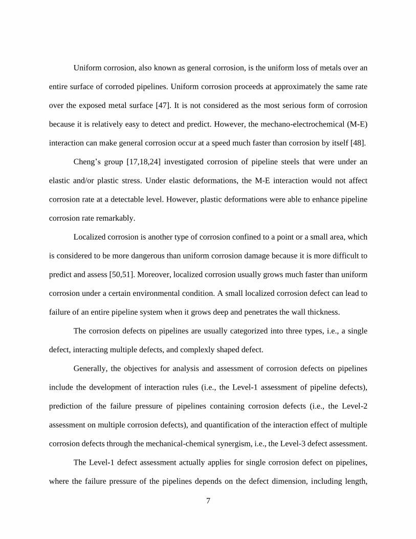
21

2 31.12 1

13

f y d

d

t tP F TdD

t M

−

= −

(2.2)

where y is the yield stress, F is design factor (normally 0.72), and Td is the temperature derating

factor (usually 1). The current ASME B31.8 code gives no derating of line pipe steels for

temperature below 250°F. For pipeline steels in the Grade X60-X70 range, data show that a

reduction of the yield strength may be exhibited at temperatures below 250°F in some cases. The

factor M is defined as

2

1 0.8L

MD t

= +

(2.3)

For longer corrosion areas, the approximation of a parabolic shape is not appropriate. When

equation (2.4) is met, the shape is rectangular.

20L D t (2.4)

11

Fig 2.3. Assumed rectangular corroded area for longer corrosion defect [9]

For the long defects, the projected area PCA is

PCA d L= (2.5)

The failure pressure Pf of the pipeline is described by

( )221.1 1 1.1f y d y d

t dt dP F T F T

D t D

− = − =

(2.6)

The factor M approaches infinity

M → (2.7)

In summary, the AMSE B31G is a conservative method. The limitations make it impossible

to apply for varied corrosion defects, pipe materials and loading conditions. The limitations

include:

1) considers internal pressure only,

2) applies to defects with relatively smooth contours,

3) ignores the circumferential extent,

4) covers steel grades lower than X65,

5) cannot be used for thick-walled pipelines.

12

However, the method possesses an important advantage that it is easy to obtain the failure

pressure by simple calculations.

2) Modified B31G

The modified B31G standard [10,11] has been confirmed against 86 burst tests on pipelines

containing actual corrosion defects. One of the most significant changes to the original B31G

method is the approximation of defect geometry. Corrosion shape is defined by 0.85 dl.

Fig 2.4. Assumed rectangular corroded area for a long corrosion area [10]

This method removes the conservation by changing the stress limit 1.1 y to

69 MPay +（） . This is close to the conventional fracture mechanics definition of the flow stress,

i.e., the average of the yield and ultimate strengths. This modification results in the change of the

failure pressure prediction equation, which is also dependent on the defect length

50L D t (2.8)

When the L value meets equation (2.8), the failure pressure is replaced by

13

1 0.852

( 69)1

1 0.85f y

d

t tPdD

t M

−

= + −

(2.9)

The factor M is given by

2 221 0.6275 0.003375( )

L LM

D t D t= + −

(2.10)

When the axial length of the corroded area meets equation (2.11), the failure pressure equation

remains the same, but M changes.

50L D t (2.11)

2

3.3 0.032L

MD t

= +

(2.12)

2.2.2 Failure pressure prediction by finite element modeling

Xu and Cheng [49] developed a FE based model to predict failure pressures of X65 and

X80 steel pipelines containing a single corrosion defect with varied depths. It was found that the

defect induced a local stress concentration, which was increased with the increasing depth of the

defect (while its width was unchanged). Su et al. [52] developed a FE model to predict failure

pressures of corroded pipelines by considering the pipe steel grades and geometries of corrosion

14

defects. The results indicated that, for short and deep corrosion defects, the failure pressures were

sensitive to the corrosion width. Thus, the effect of the defect width on the failure pressure of

pipelines should be considered in assessment methods. Generally, for corrosion defects with

similar length and width, the alignment with the longitudinal or circumferential direction does not

obviously affect the failure pressure of pipelines. However, at a given depth, if the defect length

and its width are greatly different, the orientation of corrosion defects, i.e., longitudinally or

circumferentially, would apparently influence the failure pressure. Moreover, the defect length

influences the failure pressure more greatly than the width at a given depth [53].

2.2.3 M-E effect

The mechano-electrochemical (M-E) effect refers to accelerated electrochemical reactions,

such as corrosion, by mechanical action, proposed by Gutman [30]. Multi-physics fields exist on

metal surface to affect (usually increase) the corrosion process in service environments. The M-E

effect has been investigated extensively in stress corrosion of steels [55–61]. It is commonly

accepted that the corrosion resistance of metals is reduced by mechanical stress/strain, resulting in

an increased corrosion rate. The corrosion enhancement associated with plastic deformations is

much more apparent than elastic one. Based on Gutman’s theory, Cheng developed a mechano-

electrochemical (M-E) effect concept used in pipeline corrosion [32]. It was demonstrated that, for

a single corrosion defect on pipelines, the effect of local elastic deformations on both corrosion

thermodynamics and kinetics at the defect is negligible, compared to that induced by plastic

deformations. Under the M-E effect, the region with a high stress, such as the defect center, could

serve as an anode, and that under a low stress, such as the sides of the defect, as the cathode.

Anodic dissolution at the defect center was accelerated. The corrosion at the defect center was

15

further enhanced by the increasing depth of the corrosion defect. In addition, hydrogen, once

penetrated into the steel, can increase the electrochemical activity and corrosion rate in aqueous

environments, and also affects the local stress concentration. Extensive experimental tests have

been conducted on pipeline steels to demonstrate the reliability of the concept [19–21,36,38].

Moreover, Xu and Cheng [37] developed a FE model to simulate and predict the time-

dependent growth of corrosion defects on a X100 steel pipeline in a near-neutral pH solution. The

remaining service life and failure risk of corroded pipelines were investigated. The corrosion-

resulting geometrical change of corrosion defects elevates the local stress concentration, which

again accelerates the corrosion reaction. In the long term, in the absence of the M-E effect, the

defect uniformly grows in both depth and width directions. However, the presence of the M-E

effect results in a rapidly increasing stress concentration and anodic current density at the defect

over time. The defect growth rate at the depth direction is higher than that in the width direction,

resulting in generation of a triangular shaped flaw, and the crack would be initiated at the defect

center [48].

2.2.4 Other studies

The buried pipelines are under complex stressing condition. In addition to the hoop stress

resulted from the internal pressure, the pipelines also experience significant axial stress due to

pipe-soil interaction, especially at the instable geological areas. Earthquake, soil subsidence,

landslide, surface loading, etc. can generate axial stress on the pipelines [21,22]. From the stress

analysis perspective, the effect of axial stress on the mechanical response of structures has been

investigated [32,42,58]. For example, Tatsuro et al. [63] and Nakai et al. [64] found that the

ultimate strength of a steel plate containing corrosion pits decreased with the increasing degree of

16

pitting intensity. Zhang et al. [65] studied the influences of the shape, distribution status and the

depth of corrosion pits on the ultimate strength of corroded steel plates. Wang et al. [66] conducted

numerical analyses on steel structures with random corrosion pits and found that the plasticity

initiated at the unload edge of the structures and propagated towards the plate center from the

edges.

2.3 Multiple corrosion defect

2.3.1 Overview of multiple corrosion defects

Colonies of corrosion defects are frequently found on pipelines. Usually the failure of

pipelines containing a colony of closely spaced corrosion defects is much more complex than those

containing the same defects that are isolated. This phenomenon is due to the interaction between

adjacent corrosion defects. Efforts have been made to study the failure behaviors and assess

pipelines containing interacting corrosion defects [43,45,67–73]. The largest part of the work has

focused on two aspects. The first is the determination of the interaction identification rule, and the

second is the failure pressure prediction of pipelines containing interacting defects. Normally, the

failure pressure of a pipeline containing a colony of closely spaced corrosion defects is smaller

than that when the defects are isolated. Each corrosion defect causes disturbance in the stress and

strain fields that spread out beyond the defect on the pipeline. When the influencing areas of

adjacent defects are overlapped, the failure pressure can be lower. A number of models have been

proposed to analyze the effects induced by corrosion defects and predict the failure pressure of

pipelines [43–45,67,68].

The multiple corrosion defects can be categorized into three types, including longitudinally

aligned, circumferential aligned and overlapped corrosion defects.

17

Compared to the longitudinally aligned corrosion defects, the circumferentially aligned

defects have not been paid much attention by date, which is due to the claims made from some

work that the interaction between circumferential defects is not significant. In the early 1990s, it

was reported that corrosion pits did not interact in the circumferential direction [70,74]. Later, it

was claimed that the mutual interaction of circumferential aligned defects could be ignored [31-

34]. Al-Owaisi et al. [79] proposed that the distance in the longitudinal direction between multiple

corrosion defects played a more important role in pipeline failure than the distance in the

circumferential direction.

The existing evaluation methods do not apply when multiple corrosion defects overlap each

other. In reality, corrosion defects are frequently overlapped on the pipelines. Investigation of the

overlapped corrosion defects often relies on the finite element analysis.

2.3.2 Interaction rules

The interaction between each pair of corrosion defects with a colony of defects is controlled

by a number of parameters, including the spacing (S) between them, the pipe outer diameter D, the

pipe wall thickness t, the depth of the defects (d1 and d2), the length of the defects (L1 and L2) and

the width of the defects (w1 and w2). Among these parameters, the spacing between defects is

critical to affect the existence of the interaction of the defects.

The majority of the existing rules for interaction of corrosion defects are empirically

expressed by [44]

( ) and ( )L L C C LimLimS S S S (2.13)

18

According to equation (2.13), two individual corrosion defects interact when the longitudinal

spacing between the defects is smaller than or equals to the limit value ( )L LimS and the

circumferential spacing is smaller than or equal to the limit value ( )C LimS . The most well-known

rules include the CW rule [5], DNV rule [6], 6WT rule [7] and 3WT rule [8].

The CW rule was proposed by Coulson and Worthingham in 1990. According to this rule,

the limit values ( )L LimS and ( )C LimS are calculated by

( ) 1 2

1 2

min( , )

( ) min( , )

L Lim

C Lim

S L L

S w w

(2.14)

The interaction rule recommended by the DNV-RP-F101 was proposed by Fu and Batte in

1999. The limit values of ( )L LimS and ( )C LimS are calculated as

( ) 2.0

( )

L Lim

C Lim

S Dt

S Dt

(2.15)

The 6WT rule is a commonly used interaction rule, where the limit values of ( )L LimS and

( )C LimS are calculated as

( ) 6

( ) 6

L Lim

C Lim

S t

S t

(2.16)

19

The 3WT interaction rule was proposed by Hopkins and Jones in 1992. The limit values of

( )L LimS and ( )C LimS are calculated as

( ) 3

( ) 3

L Lim

C Lim

S t

S t

(2.17)

2.3.3 Failure pressure prediction for multiple corrosion defects

When multiple corrosion defects are located at a sufficiently close spacing, their mutual

interactions further reduce the burst pressure capacity of the corroded pipeline, compared to that

containing spatially separated defects [43,69,70,72,73]. An accurate determination of the pressure

bearing capacity of pipelines containing corrosion defects is critical to the safety of the system.

The degradation of burst strength capacity of steel pipelines caused by multiple interacting

corrosion defects has been studied from a mechanical perspective [61–64]. Full scale burst tests,

combined with finite element (FE) method, were conducted to study the interaction of corrosion

defects in the early 1990s [2, 14], where it was claimed that corrosion defects did not interact in

the circumferential direction. Efforts have been made to determine appropriate separations

between defects to be considered non-interacting, and a number of codes, standards, and

engineering models have been established in the area [5, 6, 15–22].

The available rules do not include the steel strength in determination of the interaction of

corrosion defects. Therefore, the influence of the grade of pipeline steels on the interaction between

corrosion defects has not been considered. There have been so far rare investigations on overlapped

corrosion defects, which are actually more common in terms of the defect scenarios on pipelines

than the longitudinal and circumferential defects.

20

2.3.4 M-E effect

The mutual interaction between corrosion defects affects not only the mechanical stress,

but also the electrochemical corrosion, as demonstrated both experimentally and numerically [23-

29]. Wang et al. [57] studied the interaction of corrosion pits under the M-E effect using a cellular

automaton FE model but considered a consistent tensile stress only. Actually, pipelines are always

operated under a complex multi-axial stress condition. To date, no M-E numerical model has been

available to simulate corrosion colony under the realistic condition. Interaction rules are important

for identification of the interaction of multiple corrosion defects, but all the existing ones are

established based on the stress field only. The defect geometry (i.e., depth, width and length) and

their spacing affect the resulting M-E effect, but none has been investigated. Therefore, the

interaction rule used for assessment of the corrosion defects should include the M-E effect into

consideration.

2.4 Dent of pipeline

Mechanical defects present on pipelines pose a potential threat to the structural integrity

[1]. Dents, a common type of pipeline defect introduced during construction and excavation

activities, are defined as permanent inward plastic deformations on the pipe wall. Dents are stress

and strain concentrators, where cracks can be initiated with time. At the same time, dents could

obstruct the passage of in-line inspection (ILI) tools.

Generally, dents on pipelines are categorized into three types: plain dents, one dent

containing other defects, and one dent adjacent to other defects.

21

2.4.1 Plain dents

In the past decades, industry standards and models have been developed for dent

assessment, especially for plain dents [1-10]. Plain dents are smooth dents that contain no wall

thickness reductions or other defects. Plains dents are usually less dangerous to pipeline integrity

than the other two types of dent. Normally, plain dents do not cause serious risk to pipelines unless

the dents are sufficiently deep [99,102–108]. As specified in both Canadian Standard Association

(CSA) Z662 [109] and ASME B31.4 [110] standards, a plain dent is considered acceptable when

its depth is less than 6% of the pipe outer diameter. The depth-based criteria, however, were found

to be conservative [111,112]. The strain-based criteria were thus proposed. According to ASME

B31.8-2010 [113], a dented pipeline must be repaired when the dented area reaches to 6% of the

pipe limit strain. However, the formula just considered a few parameters of the dent, rather than

the dent’s entire profile. As compared to the industry standards and methods, finite element

analysis (FEA) provides an effective tool to evaluate the local strain of the dent with consideration

of its actual shape. For example, Woo et al. [100] conducted FEA on the shape and size of dents

identified by ILI tools, and proposed recommendations to quantify the error about the dent

geometry between the ILI data and FE modeling profiles.

Statistics showed that, of 75 burst tests conducted on the pipes containing unconstrained

plain dents from 1958 to 2000, only four were failed at the dented area [98]. The failures usually

occurred on other places than the dent, which is associated with the increased ultimate tensile

strength of the steel at the dented area by the so-called strain hardening. The exception is the dents

present on weld, which can have a very low burst capacity, as demonstrated by full scale tests

[106,108].

22

2.4.2 Dents containing other stress risers

Of the pipeline incidents caused by mechanical damage, 87% of the events were resulted

from development of secondary problems such as corrosion, stress corrosion cracking, etc. [114].

Therefore, a dent accompanied with other defects requires increased attention, especially for a dent

containing other stress risers such as corrosion, gouges, scratches, and cracks. It was found that

the burst strength of the dent combined with a stress riser damage becomes lower than that of either

an equivalent dent or an equivalent stress riser on an undented pipe [115,116]. CSA Z662-15

specifies that dents that contain corroded area with a depth greater than 40% of the nominal pipe

wall thickness requires repair [109]. Cai et al. [117] found that, for the combined dent with metal

loss on pipes, the dent affects the pipe residual strength more obviously than the metal loss. Tian

and Zhang [118] analyzed the scratched dents on pipelines made of X65 and X70 steels. They

found that the scratch length and depth and the dent depth are the main factors influencing the

burst pressure capacity. Cracks may be initiated at a dent due to coating failure and exposure to

corrosive environments. Ghaednia et al. [119] determined that the dent-crack defect with the crack

depth of 70% of the pipe wall thickness can reduce the failure pressure by 55%. Some models

were also proposed to predict the burst strength of pipelines containing a dent combined with a

gouge [105,106,120,121].

2.4.3 Dents interacting with the adjacent stress risers

While major efforts have been made to assess plain dents or dents containing other stress

risers, technical gaps exist regarding the integrity of pipelines containing a dent that is adjacent to

a corrosion feature. A dent that interacts with its adjacent stress riser would remarkably impact the

pipeline integrity. In addition, the mutual interaction between the dent and the corrosion feature

23

makes the assessment difficult to conduct, compromising the accuracy for prediction of the

pipeline failure pressure. Hassanien et al. [101] found that the probability of failure of a pipeline

increased when a dent interacted with corrosion features. To date, there has been no model

available to determine the burst pressure capacity of pipelines containing a dent adjacent to a

corrosion feature. Moreover, there is no criterion to evaluate whether an interaction exists between

the dent and the adjacent corrosion defect or they can simply be treated individually.

24

Chapter Three: Research methodology

3.1 FE models for failure pressure prediction of pipelines containing multiple corrosion

defects

3.1.1 Initial and boundary conditions

FE analyses in this work were performed using a software ANSYS 15.0, a general-purpose

FE modeling package for numerically solving a variety of mechanical problems. Three-

dimensional (3D) FE models were developed, enabling the determination of the failure pressure

of pipelines containing multiple corrosion defects which were oriented either longitudinally,

circumferentially or overlapped with each other. To reduce the computational cost, one quarter of

a pipe including corrosion defects was modeled considering the symmetrical nature of the

assembly, as shown in Fig. 3.1a.

Fig 3.1. 3D modeling of a pipe containing corrosion defects (a) a quarter model, (b) meshes

of a longitudinal corrosion defect, (c) meshes of a circumferential corrosion defect, (d)

meshes of two overlapped corrosion defects.

(c) (d)

25

Symmetrical constraints were applied on the planes to be modeled. Displacement in the Z

direction of the uncorroded end was also constrained. The length of the pipe was sufficient to avoid

the effect of boundary conditions on the corroded area. It is noted [70] that, when the length of the

modeled pipe exceeds 4.9 (Dt/2)1/2, where D is the diameter of the pipe, and t is the pipe wall

thickness, the boundary condition does not influence the modelling results. In this work, D is

229.4mm and t is 10 mm. 4.9 (Dt/2)1/2=234.7 mm. The length of 2000mm of the pipe is sufficient

to eliminate the effect of the boundary condition on FE modeling.

Figs. 3.1b - 3.1d show the mesh refinement applied on the corrosion defects to ensure

reliable simulation. The uncorroded area on the pipe was under coarse meshing to reduce the

computational cost. A mesh density analysis was conducted to determine the appropriate meshing

sizes for different defects, as shown in Fig. 3.2. The mesh sizes were 8 mm and 10 mm in

circumferential and longitudinal directions, respectively. The maximum and minimum element

sizes of the corroded region were 3 mm and 1 mm, respectively. The corrosion defects have a

smooth edge, with a radius equaling to the defect depth, to avoid a high stress concentration. All

the parameters were not changed over time during each simulation run as they were static

parameters.

26

0 20000 40000 60000 80000 100000 120000500

550

600

650

700

750

800

Ma

xim

um

vo

n M

ises

str

ess

(MP

a)

Number of elements


multiple corrosion defects

3.1.2 Properties of pipeline steels and the failure criterion of pipelines

Three grades of pipeline steel, i.e., API X46, X60 and X80 steels, were chosen for FE

modeling. The Ramberg-Osgood (R-O) stress-strain rule, which was widely used to describe the

hardening behavior of metals [122], was adopted in this work. The R-O equations for pipeline

steels were [123]

n

yE E

= +

(3.1)

12.64= +0.079( )uE

(3.2)

27

where ε is true strain, σ is true stress, E is Young’s modulus (200,000 MPa), y is yielding

strength, u is ultimate tensile strength, and and n are R-O material parameters. The properties

and relevant parameters of the three steels are listed in Table 3.1 [80,122,123]. Particularly, the

equation (3.1) applied for X46 [122] and X60 [123] steels, and equation (3.2) worked for X80 [80]

steel for validation of the FE modeling results. The Poisson’s ratio ( ) was set as 0.3.

Table 3.1. Properties and relevant parameters of three grades of pipeline steel.

Steel grade n y (MPa) u (MPa)

X46 [122] 7.45 3.74 357.0 542.0

X60 [123] 7.31 2.29 433.0 618.0

X80 [80] - - 534.1 718.2

The primary stress of pipelines is from internal operating pressure. The failure criterion

used in this work follows a stress-based one, where pipeline failure occurs when the von Mises

equivalent stress exceeds a reference stress level at the corrosion defects. The ultimate tensile

strength u was used as the reference stress in this work [6].

3.1.3 Validation of FE modeling results

The FE modeling results must be validated by comparison with data from various sources,

which can be a computational software that has a different analytical basis, a theoretical

calculation, or experimental data [124]. Experiment testing is sometimes time-consuming, but it is

reliable if the solution cannot be obtained theoretically and there is no previous data that can be

referred to. The verification and optimization of the FE modeling in this work were based on the

28

experimental data published in Benjamin and Cunha’s work [125], where a series of tests were

conducted to study the interaction of corrosion defects on pipelines. Relevant testing results were

chosen to validate the accuracy of the FE models developed in this work. The testing specimens

used by Benjamin and Cunha [125] were cut from a pipe made of API X80 steel, with a pipe wall

thickness of 8.1 mm and an outer diameter of 458.8 mm. As shown in Table 3.2, specimen #1 had

a single defect, while specimens #2 and #3 were both composed of two corrosion defects with

similar geometries. The defects on specimen #2 were longitudinally aligned along the axis of the

pipe. For specimen #3, two corrosion defects were circumferentially aligned and perpendicular to

the axis of the pipe. The defects were all machined in the laboratory.

Table 3.2. Geometry of corrosion defects present on pipelines published in Benjiamin’s

work [125]

Specimen

Defect depth

(mm)

Defect length

(mm)

Defect width

(mm)

SL

(mm)

SC

(mm)

Defect

orientation

#1 5.39 39.60 31.90 - -

#2 5.32 39.60 31.90 20.50 -31.90

#3 5.62 39.60 32.00 -39.60 9.90

For a single corrosion defect and two defects longitudinally or circumferentially aligned

on an X80 steel pipeline, as shown in Table 3.2, the failure pressures determined by FE modeling

in this work, PFEM, are listed in Table 3.3, where the testing failure pressures (PE) [68] are also

included for comparison. The variation between the two sets of failure pressure is calculated by

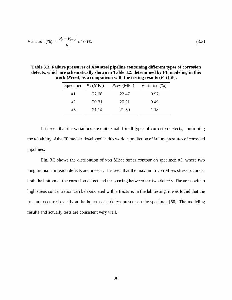
29

Variation (%) = 100%E FEM

E

P P

P

− (3.3)

Table 3.3. Failure pressures of X80 steel pipeline containing different types of corrosion

defects, which are schematically shown in Table 3.2, determined by FE modeling in this

work (PFEM), as a comparison with the testing results (PE) [68].

Specimen PE (MPa) PFEM (MPa) Variation (%)

#1 22.68 22.47 0.92

#2 20.31 20.21 0.49

#3 21.14 21.39 1.18

It is seen that the variations are quite small for all types of corrosion defects, confirming

the reliability of the FE models developed in this work in prediction of failure pressures of corroded

pipelines.

Fig. 3.3 shows the distribution of von Mises stress contour on specimen #2, where two

longitudinal corrosion defects are present. It is seen that the maximum von Mises stress occurs at

both the bottom of the corrosion defect and the spacing between the two defects. The areas with a

high stress concentration can be associated with a fracture. In the lab testing, it was found that the

fracture occurred exactly at the bottom of a defect present on the specimen [68]. The modeling

results and actually tests are consistent very well.

30

Fig 3.3. Distribution of von Mises stress (MPa) contour of specimen #2, where two

longitudinal corrosion defects are present.

3.1.4 FE modeling of longitudinally and circumferentially aligned, as well as overlapped

corrosion defects

As mentioned above, the FE modeling conducted on specimens #2 and #3 was performed

to determine the interaction between two longitudinally and circumferentially aligned corrosion

defects, respectively, but the steel was of X80 grade only [80]. Models were thus developed for

the grades of X46 and X60 steels in this work, and further, the failure pressure of corroded

pipelines was predicted under various longitudinal and circumferential spacing between adjacent

corrosion defects.

In addition to longitudinally and circumferentially aligned corrosion defects, multiple

corrosion defects overlapped with each other were also modeled to be representative of the reality

in this work. FE models were developed to study the interaction of overlapped, two layers of

corrosion defects present on three grades of steel. The outer pipe diameter was 458.8 mm, and the

31

wall thickness was 10.0 mm. Fig. 3.3 shows the FE model for the overlapped corrosion defects.

The top (or big) defect was defined as the first layer defect with the half length, depth and half

width of L1, d1 and w1, respectively. The bottom (or small) defect was defined as the second layer

one with the half length, depth and half width marked as L2, d2 and w2, respectively. Same as the

longitudinal and circumferential defects, the overlapped ones were rectangularly shaped. The

lengths (L1 and L2) were always in the axial direction of the pipe, and the widths (w1and w2) were

in the circumferential direction. The half angular width, w1 and w2, were 16° and 8°, respectively.

The values of L1 to be modeled included 19.8 mm, 39.6 mm and 79.2 mm, and L2 was a half of L1.

The values of d1 were 2 mm, 3 mm and 4 mm, and those of d2 were 0.3, 0.4, 0.5, 0.6, 0.7, 0.8, 0.9

and 1.0 time of d1, respectively. In reality, the size of corrosion defects may change during the

corrosion process. In this work, it was assumed that the corrosion defect maintained at a fixed

width, with growing depth and length in order to investigate the mutual influence of the overlapped

defects in the depth and length directions. Actually, it was proven that compared to the defect

length and depth, the width did not affect apparently the interaction of defects [126].

32

Fig 3.4. FE model of a pipe containing two corrosion defects overlapped with each other.

The top (or big) defect has a length of 2L1, depth d1 and width 2w1, and the bottom (or

small) defect has a length of 2L2, depth d2 and width 2w2.

It is noted that the dimensions of the corrosion defects simulated in this work are well

within the size ranges of actual defects present on pipelines. According to the AGA/PRCI Database

of Corroded Pipe Tests [126], the actual corrosion defects detected on pipelines usually have a

range of dimension of 19.35 to 3048.00 mm in length, 1.60 to 17.10 mm in maximum defect depth,

and 0.15 to 304.80 mm in width. The simulated corrosion defects in this work are ranged as the

length of 39.60 to 158.40 mm, the defect depth of 0.60 to 5.62 mm, and the width of 19.80 to 39.60

mm.

3.2 FE models for simulation and prediction of the M-E effect at multiple corrosion defects


The multi-physics FE modeling of the M-E interaction of corrosion defects on an X46 steel

pipeline was conducted using a commercial COMSOL Multiphysics® 4.2a software [127]. A

relative tolerance of 0.001 was adopted to assure the convergence. A half of the steel pipe

containing multiple corrosion defects was simulated by a 3-D model, as shown in Fig. 3.5, to

reduce the implementation complexity and computational cost considering the symmetry of the

object. For comparison, a 2-D model was used to simulate the stress, potential, and current density

distributions on the pipe under an axial stress. The pipe wall thickness (t) was 10 mm, and the

outer diameter (D) was 458.8 mm. The length of the pipe segment for FE simulation was 2,000

mm. All the parameters were not changed over time during each simulation run as they were static

parameters.

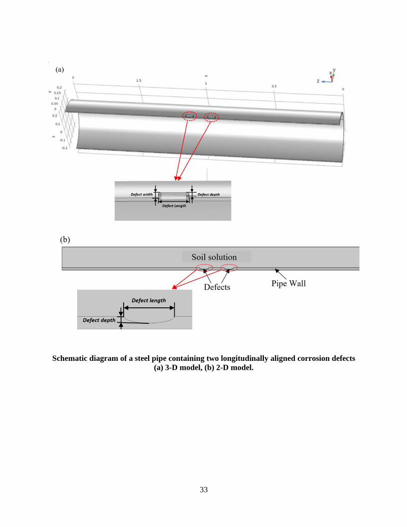
33

Schematic diagram of a steel pipe containing two longitudinally aligned corrosion defects

(a) 3-D model, (b) 2-D model.

34

(a)

(b)

Schematic diagram of a steel pipe containing two circumferentially aligned corrosion

defects, (a) 3-D model, (2) the pipe under internal pressure or tensile stress

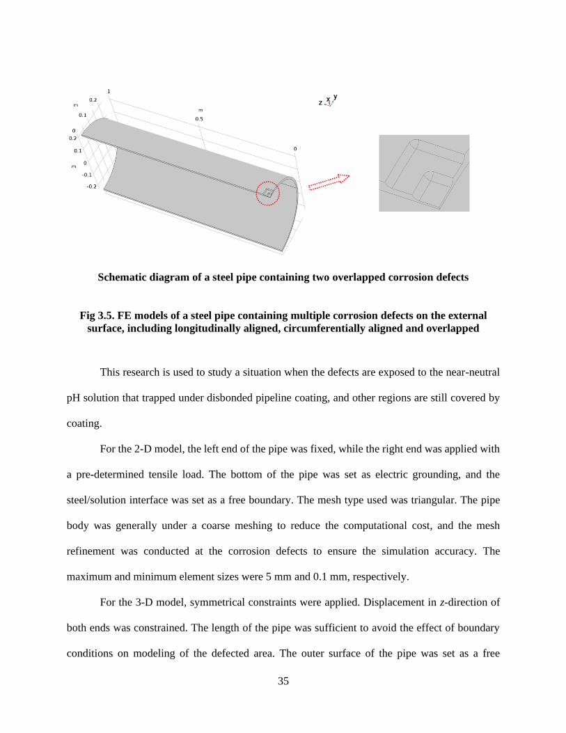
35

Schematic diagram of a steel pipe containing two overlapped corrosion defects

Fig 3.5. FE models of a steel pipe containing multiple corrosion defects on the external

surface, including longitudinally aligned, circumferentially aligned and overlapped

This research is used to study a situation when the defects are exposed to the near-neutral

pH solution that trapped under disbonded pipeline coating, and other regions are still covered by

coating.

For the 2-D model, the left end of the pipe was fixed, while the right end was applied with

a pre-determined tensile load. The bottom of the pipe was set as electric grounding, and the

steel/solution interface was set as a free boundary. The mesh type used was triangular. The pipe

body was generally under a coarse meshing to reduce the computational cost, and the mesh

refinement was conducted at the corrosion defects to ensure the simulation accuracy. The

maximum and minimum element sizes were 5 mm and 0.1 mm, respectively.

For the 3-D model, symmetrical constraints were applied. Displacement in z-direction of

both ends was constrained. The length of the pipe was sufficient to avoid the effect of boundary

conditions on modeling of the defected area. The outer surface of the pipe was set as a free

36

boundary, while other surfaces were set as electrically isolated. The mesh type was tetrahedral.

Similarly, the pipe body was under a coarse mesh, and the meshing refinement was applied on the

defected area. The maximum and minimum element sizes were 10 mm and 1 mm, respectively.

The length of the pipe was sufficient to avoid the boundary effect on corroded region. The mesh

sensitivity analysis is shown in Fig. 3.6. The FE simulation was conducted in three physical fields,

i.e., mechanical stress field, electrochemical corrosion field, and M-E coupling field.

Fig 3.6. Mesh sensitivity analysis for M-E effect of an X46 pipe containing multiple

corrosion defects

3.2.2 Properties of pipeline steels and electrochemical corrosion parameters

X46 pipeline steel was used for FE modeling in this work. The elastic properties of the

steel included a Young’s modulus (E) of 207,000 MPa and a Poisson’s ratio ( ) of 0.3. The plastic

stress follows a nonlinear isotropic hardening model [32]

0 10000 20000 30000 40000 50000 60000 700000

100

200

300

400

500

600

700

Maximum von Mises stress

Maximum anodic current density

Number of elements

Maxim

um

von M

ises s

tress (

MP

a)

5.0

5.2

5.4

5.6

5.8

6.0

Anodic

curre

nt d

ensity

(A

/cm

2)

37

σ = σys + σh ϵps (3.4)

where σys is yield strength, i.e., 410 MPa for X46 steel [39], σh is an experimental stress function,

and ϵps is effective plastic strain. The ultimate tensile strength of X46 steel is 630.1 MPa [39].

During corrosion, the anodic and cathodic reactions of X46 steel in the deoxygenated, near-

neutral pH solution (pH 6.8) included the iron oxidation and hydrogen evolution [32]

Anodic reaction: 2Fe Fe 2e+→ + (3.5)

Cathodic reaction: 2H+ + 2e → H2 (3.6)

It was demonstrated that the corrosion of X46 steel in the solution was activation-

controlled. The corrosion kinetic equation can be expressed as

0, exp( )aa a

a

i ib

= (3.7)

0, exp( )cc c

c

i ib

= (3.8)

eq = − (3.9)

where 0,ai and 0,ci are anodic and cathodic exchange current densities, respectively, ai and ci are

anodic and cathodic current densities, respectively, a and c are anodic and cathodic

38

overpotentials, respectively, ab and cb are anodic and cathodic Tafel slopes, respectively, is

electrode potential, and eq is equilibrium electrode potential. According to Nernst equation, the

anodic and cathodic equilibrium potentials are written as

0 2

, ,

0.0592log Fe

2a eq a eq + = + (3.10)

0

, , 0.0592log[H ] 0.0592pHc eq c eq += + = − (3.11)

The equilibrium potentials of reactions (3.10) and (3.11) are calculated as -0.859 V (saturated

calomel electrode, SCE) and -0.644 V (SCE), respectively [39]. The exchange current densities of

the two reactions are derived from the group’s previous work [39]. Table 3.4 lists the

electrochemical corrosion parameters used as the initial inputs for FE modeling in this work.

Table 3.4. The initial electrochemical parameters for FE simulation derived from [39]

Electrochemical

reactions

log i0

(A/cm2)

Equilibrium

potential

(V, SCE)

Tafel slope

(V/decade)

i0

(μA/cm2)

Hydrogen evolution -5.989 -0.644 -0.192 1.026

Iron oxidation -6.359 -0.859 0.111 4.373×10-1

39

3.2.3 Effect of stress on electrode potential

According to Gutman’s theory [128], the change of equilibrium electrode potential

caused by external elastic and plastic deformations can be expressed as:

Elastic deformation: ,

e ma eq

PV

zF

= − (3.12)

Plastic deformation: ,

0

ln( 1)p

a eq p

TR

zF N

= − + (3.13)

where ,

e

a eq and ,

p

a eq denote variations of equilibrium potential of anodic reaction under elastic

and plastic deformations, respectively, 0

,a eq is the standard equilibrium potential of anodic

reaction, mV is molar volume (for steel, 6 37.13 10 m / mol− ), z is charge number (i.e., 2 for steels),

R is ideal gas constant (8.314 J / mol K ), T is absolute temperature (298.15 K), F is Faraday’s

constant (F = 96485 C/mol), is an orientation-dependent factor ( 0.45 = ), is a coefficient

(i.e., 11 21.67 10 cm− ), 0N is the initial dislocation density prior to plastic deformation ( 8 21 10 cm− ),

p is plastic strain obtained from solid mechanics simulation [128], and P equals to 1/3 of

uniaxial tensile stress in 2-D model; while in 3-D model, it is expressed as:

( ) / 3zP = + (3.14)

2

PD

t = (3.15)

4z

PD

t = (3.16)

40

where is hoop stress, z is axial stress, P is internal pressure, D is outer diameter of pipeline,

and t is pipe wall thickness. The equilibrium potential of the anodic reaction under the M-E effect

can thus be written as:

0

, ,

0

ln( 1)m ma eq a eq p

P V TR

zF zF N

= − − + (3.17)

3.2.4 Comparison of 3D modeling results with the theoretical calculations

The modeling results obtained in this work were validated by theoretical calculations of

both the first principal stress in solid mechanics field and the anodic current density in

electrochemical corrosion field on an X46 steel pipeline. The anodic dissolution current density,

ai , of an elastically stressed steel is given by [54].

exp( )ma a

PVi i

RT

= (3.18)

whereai is the anodic current density of a non-stressed steel in an aqueous solution.

The anodic current density (A/m2) and corrosion rate (CR) are related by CR=3.06 zρ/M

(A/m2), where z is number of electrons exchanged in corrosion reaction, ρ is density (g/cm3), and

M is atomic mass (g) [47]. For steels, z=2, ρ=7.88 g/cm3, and M=55.85 g. Thus, the relation of 1

mm/y=0.863 A/m2 applies for corrosion rate conversion for steels.

Table 3.4 shows the first principal stress and anodic current density of X46 pipeline steel

in the near neutral pH NS4 solution under various internal pressures, as compared with the

modeling results obtained in this work. It is seen that the variations between the theoretical

41

calculations and modeling results are below 10 %, indicating the reliability of the developed model

for the M-E effect determination. The differences can be occurred by the boundary conditions and

element type.

Table 3.5. First principal stress (MPa) and anodic current density (μA/cm2) of X46 steel

pipe in a near neutral solution under various internal pressure determined by FE modeling

in this work, as a comparison with the theoretical calculations.

3.3 FE models for failure pressure prediction of pipelines containing a corrosion defect

associated with a dent


A general-purpose software package ABAQUS 6.13 was used in this work to perform FE

analysis. 3D FE models of a pipe segment and a rigid indenter shaped of a ring torus [100] were

created for modeling the formation of a dent on the pipe. The pipe outer diameter was 762 mm,

and the wall thickness was 6.35 mm. The dent was created by the indenter, introducing an inward

deformation on the pipe wall. In order to model the denting procedure, a contact algorithm was

chosen in ABAQUS. A surface-to-surface contact method was employed between the pipe and the

Internal Pressure (MPa) 2 3 4 5 6 7 8 9 10

First

principle

stress,

(MPa)

Theoretical 45.88 68.82 91.76 114.70 137.64 160.58 183.52 206.46 229.40

Simulation 45.86 68.80 91.75 114.70 137.60 160.55 183.50 206.44 229.38

Variation

(%) 0.04 0.03 0.01 0 0.02 0.02 0.01 0.01 0.01

Anodic

current

density,

ai 2(μA/cm )

Theoretical 3.92 4.08 4.14 4.32 4.51 4.60 4.81 4.96 5.14

Simulation 3.90 4.07 4.13 4.29 4.48 4.57 4.80 4.95 5.12

Variation

(%) 0.51 0.25 0.24 0.69 0.67 0.65 0.21 0.20 0.39

42

indenter. Since the indenter is much harder than the pipe steel, the indenter was selected as the

master surface and the pipe as the slave surface.

Fig 3.7. (a) 3D modeling of a pipe containing a dent and corrosion feature, (b) a dent

located adjacently to corrosion feature.

The dent was introduced into the pipe when it is idle (i.e., at zero pressure), modelling the

dent generation during construction of the pipeline. Three steps were taken for the entire simulation

process. The pipe was firstly dented by the rigid indenter with a specific amount of indentation.

Then the indenter was removed, and a phenomenon of “spring back” was observed at the dented

area during the indenter-removal. The dented pipe was finally pressurized until the maximum von

Mises stress reached the ultimate tensile strength of X46 steel (i.e., 630MPa). The dent was re-

rounded with the increased internal pressure. The corrosion feature was developed with the

technique of element deactivation after the indenter was removed. This approach could simulate

(a)

(b)

43

the corrosion feature on the pipe body after the dent formation. Symmetrical conditions permitted

modelling of one-half of the pipe segment for reducing computational time. The pipe length was

enough to avoid the effect of boundary conditions on the dented and corroded regions. The dent

and the adjacent corrosion feature were longitudinally located on the pipe surface, as shown in Fig.

3.7.

Fig 3.8. (a) Meshes of pipe and indenter, (b) refined mesh of damaged area, (c) symmetrical

constraints.

(a)

(b)

(c)

44

A 3D 8-node linear brick (C3D8R), reduced-integration solid element was assigned on the

pipe body, enabling a large deformation and contact analysis. The indenter was composed of a 4-

node linear doubly curved shell (S4R), with reduced-integration element. Three elements were

assigned over the wall thickness of the pipe. Fig. 3.8a shows the meshes of the pipe and the indenter.

The mesh was assigned equally along the circumferential direction with the size of 30 mm. In the

longitudinal direction of the pipe, the mesh size was assigned increasingly from the dented region

to the pipe end with a single bias mesh strategy, starting from 2 mm to 30 mm. The mesh was

refined at the dented and corroded regions, as shown in Fig. 3.8b. Kinematic coupling constraint

with freedom in the radial direction boundary condition was applied on both ends of the pipe with

the fixed center points, allowing the pipe to expand at the center points with increased internal

pressures, but no rigid body motion. Symmetrical constrains were applied on two symmetrical

longitudinal planes, as shown in Fig. 3.8c.

The dent depth, and the length and depth of the corrosion feature were considered in the

modelling. The dent depths were 4.1, 11.4 and 20.0 mm. The corrosion length varied between 50

mm and 150 mm, and the corrosion depth increased from 25% to 78% of the pipe wall thickness,

with a fixed corrosion width. Previous work demonstrated that the corrosion width was not as

important as the corrosion length and depth to affect the failure pressure of corroded pipelines

[129]. Round edges with a radius equaling to the corrosion depth were made on the corrosion

feature to relieve the stress concentration. All the parameters were not changed over time during

each simulation run as they were static parameters.

45

3.3.2 Properties of pipeline steels

The X46 pipeline steel used for the FE modelling in this work possesses a Young’s

modulus, E , of 207,000 MPa and Poisson’s ratio, , of 0.3. The stress-strain relationship was

obtained previously [39], where the yielding strength was 410 MPa and the ultimate tensile

strength was 630.1 MPa. The isotropic hardening of the steel was used in the modelling.

The failure criterion of pipelines follows the von Mises yield criterion, where the pipeline

failure occurs when the von Mises equivalent stress exceeds a reference stress level at the defective

area. In this work, the reference stress was the ultimate tensile strength of X46 steel.

3.3.3 Mesh density analysis

A mesh density analysis was conducted to optimize the meshing selection to obtain reliable

modelling results with the least time frame. The mesh sizes used were 100 mm, 50 mm, 30 mm,

20 mm and 10 mm, following the hoop direction. The total number of elements used in each pipe

segment was 20,550, 24,454, 27,152, 31,538 and 49,144 for the 100 mm, 50 mm, 30 mm, 20 mm

and 10 mm meshes, respectively. The modelled maximum von Mises stress for each element size

is shown in Fig. 3.9. By consideration of the modelling accuracy and computational time, the 30

mm element size (i.e., 27,152 elements) for the hoop direction was selected. The dented and

corroded regions were assigned with elements with the size of 2 mm. The indenter was meshed

with a bigger element size than the defective region.

46

20000 30000 40000 50000 60000600

610

620

630

640

650

Ma

xim

um

vo

n M

ises

str

ess

(MP

a)

Number of elements


dent associated with corrosion defects

47

Chapter Four: Modeling of the interaction of multiple corrosion defects and its effect on

failure pressure of pipelines1

4.1 Interaction of longitudinally and circumferentially aligned corrosion defects on

pipelines

As stated, the interaction between adjacent corrosion defects results in decreased failure

pressure of pipelines. To quantify the interaction, the failure pressure of a pipeline containing a

single defect, i.e., Psingle, determined by the FE analysis, is used as a reference. The criterion used

to evaluate the interaction between corrosion defects is defined as [67]

/ 0.99, no interaction

/ 0.99, interaction exists

multiple single

multiple single

P P

P P

(4.1)

where Pmultiple is the failure pressure of pipelines containing multiple corrosion defects. When the

ratio of Pmultiple/Psingle equals to or larger than 0.99, there is no interaction between the adjacent

defects. If the ratio is smaller than 0.99, an interaction exists between the defects. The ratio of 0.99

allows for a certain tolerance. The smaller the ratio, the more significant the effect of interaction

on failure pressure of pipelines is.

The effect of the longitudinal spacing of corrosion defects is conducted on specimen #2

listed in Table 3.2, where the depth, length and width of the defects are 5.32 mm, 39.60 mm and

31.90 mm, respectively. Two defects are aligned longitudinally in the axial direction of the pipe.

1 The research work in this chapter is published as:

Jialin Sun, Y. Frank Cheng, Assessment by finite element modeling of the interaction of multiple corrosion defects

and the effect on failure pressure of corroded pipelines, Engineering Structures 165 (2018) 278-286.

48

The spacing of the defects refers to the distance between the adjacent edges of the defects. Fig. 4.1

shows the effect of the longitudinal spacing of corrosion defects on the ratio of failure pressures

(Pmultiple/Psingle) of pipelines made of X46, X60 and X80 steels. It is seen that the ratio of

Pmultiple/Psingle increases with the increasing longitudinal spacing between the corrosion defects.

This indicates that the effect of interaction on the failure pressure of corroded pipelines reduces as

the longitudinal spacing of the defects increases. There is little effect of the steel grade on the

change of the Pmultiple/Psingle ratio vs. the longitudinal spacing between defects. A critical

longitudinal spacing value of 152.40 mm is identified for the three grades of pipeline steel as the

failure pressure ratio of three curves all reaches 0.99.

In summary, for pipelines containing longitudinally aligned corrosion defects, when the

spacing between them is larger than 152.40 mm, the interaction does not exist, and the multiple

defects can be treated as individual ones. The steel grade does not affect this conclusion.

0 20 40 60 80 100 120 140 160 180 2000.87

0.90

0.93

0.96

0.99

1.02

Pm

ult

iple/P

sin

gle

Longitudinal spacing (mm)

X46

X60

X80

0.99

Fig 4.1. Effect of the longitudinal spacing of corrosion defects on the ratio of failure

pressures (Pmultiple/Psingle) of pipelines made of X46, X60 and X80 steels.

49

The effect of the circumferential spacing of corrosion defects is conducted on specimen #3

in Table 3.2, where the depth, length and width of the defects are 5.62 mm, 39.60 mm and 32.00

mm, respectively. Two defects are aligned circumferentially on the circumferential direction of

the pipe. The spacing of the defects also refers to the distance between the adjacent edges of the

defects. Fig. 4.2 shows the effect of the circumferential spacing of corrosion defects on the ratio

of failure pressures (Pmultiple/Psingle) of pipelines made of X46, X60 and X80 steels. The failure

pressure ratio of three grades of pipeline steel also increases with the increasing circumferential

spacing between corrosion defects, indicating that the interaction of the defects reduces with the

increasing circumferential spacing. Similar to the longitudinal defects in Fig. 4.1, the steel grade

affects slightly the dependence of the failure pressure ratio on the circumferential spacing. Thus,

the interaction between circumferential defects is also approximately independent of the grade of

pipeline steel. The three curves reach the critical ratio at the circumferential spacing of about 43.2

mm, which is much smaller than the critical spacing for longitudinal defects.

50

0 20 40 60 80 100 120 140 160 180 2000.984

0.986

0.988

0.990

0.992

0.994

Pm

ult

iple/P

sin

gle

Circumferential spacing (mm)

X46

X60

X80

0.99

Fig 4.2. Effect of the circumferential spacing of corrosion defects on the ratio of failure

pressures (Pmultiple/Psingle) of pipelines made of X46, X60 and X80 steels.

In summary, for pipelines containing circumferentially aligned corrosion defects, when the

spacing between them is larger than 43.20 mm, the interaction does not exist, and the multiple

defects can be treated as individual ones. The interaction between circumferential defects is

approximately independent of the grade of pipeline steels. Compared to circumferential corrosion

defects, the longitudinal defects are associated with a larger spacing where the interaction between

defects exists and affects the failure pressure of pipelines. Thus, the circumferential spacing of

corrosion defects has smaller of an influence on the failure pressure of corroded pipelines

compared to the longitudinal spacing of two defects with identical dimensions. The difference

between the longitudinal and circumferential spacing effects on Pmultiple/Psingle ratio is attributed to

the fact that the defect length affects the failure pressure of corroded pipelines at a more significant

51

level than the defect width while its depth is kept constant. This phenomenon was also observed

previously [126].

4.2 Interaction of overlapped corrosion defects on pipelines

Overlapped corrosion defects are aligned along the radial direction of the pipe with their

lengths in the axial direction of the pipe. Fig. 4.3 shows the distribution of von Mises stress on an

X46 steel pipe, which is representative of those on X60 and X80 steels, containing the overlapped

corrosion defects with L1 of 19.8 mm, d1 of 3 mm and various d2 values (i.e., 0.9, 1.5, 2.4 and 3.0

mm) under an operating pressure of 20 MPa. It is seen that the stress distribution is not uniform.

At individual d2, the stress inside the defects is higher than the pipe surface. With the increase of

d2, the stress at the bottom of the defects increases apparently. Thus, a stress concentration occurs

mainly at the bottom of defects as its depth increases, with the maximum von Mises stress observed

at the edge of the defects.

52

Fig 4.3. Distributions of von Mises stress on X46 steel pipe containing the overlapped

corrosion defects with L1 of 19.8 mm, d1 of 3 mm and various d2 values under an operating

pressure of 20 MPa.

Table 4.1 summarizes the failure pressures of X46, X60 and X80 steel pipelines containing

the overlapped corrosion defects with L1 of 19.8 mm and various d1 and d2/d1 ratios. It is seen that,

with other variables fixed, the failure pressure of the pipeline decreases with the increasing d1 and

d2/d1 ratio (i.e., the increasing d2 at a fixed d1). Moreover, with the fixed defect geometry, the

failure pressure of the pipeline increases with the increasing steel strength.

53

Table 4.1. Failure pressures (MPa) of pipelines containing the overlapped corrosion defects

with L1 of 19.8 mm, various d1 and the d2/d1 ratios for X46, X60 and X80 steels.

To quantify the influence of defect overlapping on the failure pressure of pipelines, the

failure pressure in the presence of a single defect, i.e., Psingle, is used as a reference. The effect of

the overlapped defects on the failure pressure of a pipeline can be described as the ratio of

Poverlapped/Psingle, where Poverlapped is the failure pressure of pipelines containing overlapped

corrosion defects. Generally, the smaller the ratio of Poverlapped/Psingle, the more significant the effect

of overlapped corrosion defects on the failure pressure. Figs. 4.4 - 4.6 show the failure pressure

ratio, i.e., Poverlapped/Psingle, of pipelines containing the overlapped corrosion defects as a function

of the depth ratio of corrosion defects, i.e., d2/d1, with L1 of 19.8 mm and L2 of 9.8 mm for X46,

X60 and X80 steels, respectively. Linear relationships are observed between the Poverlapped/Psingle

d2/d1

d1 (mm)

0.3 0.4 0.5 0.6 0.7 0.8 0.9 1.0

X46 steel

2 21.86 21.84 21.80 21.76 21.71 21.68 21.65 21.62

3 21.40 21.31 21.20 21.11 21.02 20.96 20.89 20.85

4 20.54 20.41 20.29 20.19 20.04 19.93 19.75 19.67

X60 steel

2 26.00 25.98 25.92 25.90 25.84 25.82 25.76 25.68

3 25.27 25.17 25.06 25.01 24.88 24.77 24.67 24.59

4 24.11 23.98 23.82 23.69 23.54 23.38 23.23 23.07

X80 steel

2 31.80 31.77 31.70 31.67 31.57 31.54 31.48 31.44

3 31.03 30.90 30.74 30.61 30.49 30.39 30.30 30.23

4 29.73 29.54 29.38 29.23 29.01 28.85 28.60 28.47

54

ratio and d2 /d1. This is due to the fact that the lengths and widths of overlapped corrosion defects

modeled in this work are linearly related. With varied relationships between the length and width

of the overlapped defects, the derived dependences of Poverlapped/Psingle on d2/d1 can be different.

Generally, the width (w) of corrosion defects does not greatly affect the failure pressure of

pipelines as compared to the defect depth (d) and length (L). This applies for a single defect and

multiple defects oriented either longitudinally or circumferentially [126]. It is seen that the

existence of the bottom layer defect lowers the failure pressure of the pipeline, compared to that

in the presence of a single top layer defect only. The Poverlapped/Psingle ratio linearly decreases with

the increasing d2/d1 ratio, indicating that the failure pressure decreases with the increase of d2 (i.e.,

the depth of the bottom defect) at fixed d1 values. The slope (K) of the lines obtained by the linear

regression analysis is used to quantify the relationship between the Poverlapped/Psingle ratio and the

d2/d1 ratio. Moreover, at individual d2/d1 ratios, there is a smaller Poverlapped/Psingle ratio at a larger

d1, i.e., the depth of the top layer defect. Thus, an increase in the depth of either top or bottom layer

corrosion defect would reduce the failure pressure of the corroded pipelines. A further comparison

of the absolute value of the linear slope shows that the absolute value of K increases with the

increasing d1. Thus, with the top layer corrosion defect becoming deeper, the Poverlapped/Psingle ratio

decreases more rapidly as the bottom layer defect depth increases.

55

0.2 0.4 0.6 0.8 1.0 1.20.80

0.85

0.90

0.95

1.00

1.05

K= -0.058

K= -0.036 d

1=2 mm

d1=3 mm

d1=4 mm

Fitted curve (d1=2 mm)



Poverl

apped/P

sin

gle

d2/d

1

K= -0.016


overlapped corrosion defects as a function of the depth ratio of the defects, i.e., d2/d1, with

L1 19.8 mm and L2 9.8 mm.

0.2 0.4 0.6 0.8 1.0 1.20.80

0.85

0.90

0.95

1.00

1.05

K= -0.057

K= -0.038 d

1=2mm

d1=3mm

d1=4mm

Fitted curve (d1=2mm)



Pove

rlapped

/Psi

ngle

d2/d

1

K= -0.015



L1 19.8 mm and L2 9.8 mm.

56

0.2 0.4 0.6 0.8 1.0 1.20.80

0.85

0.90

0.95

1.00

1.05

K= -0.060

K= -0.036

K= -0.014

d1=2 mm

d1=3 mm

d1=4 mm

Fitted curve ( d1=2 mm)



Po

verl

ap

ped/P

sin

gle

d2/d1



L1 19.8 mm and L2 9.8 mm.

The dependences of the Poverlapped/Psingle ratio on d2/d1 for X60 and X80 steels, as shown in

Figs. 4.5 and 4.6 are quite similar to that of X46 steel. The Poverlapped/Psingle ratio also decreases

linearly with the increasing d2/d1. Moreover, as the depth of either the top or the bottom layer

corrosion defect increases, the failure pressure of the corroded pipeline made of X60 or X80 steels

also decreases. A close comparison of the results in Figs. 4.4 - 4.6 shows that the steel grade clearly

does not affect the relationship between the Poverlapped/Psingle ratio and d2/d1, which means that the

interaction of overlapped corrosion defects is approximately independent of the strength of

pipeline steels.

57

0.2 0.4 0.6 0.8 1.0 1.20.80

0.85

0.90

0.95

1.00

1.05

K= -0.144

K= -0.094

K= -0.057

d1=2 mm

d1=3 mm

d1=4 mm




Po

verl

ap

ped/P

sin

gle

d2/d

1


pipeline with the defects’ lengths of 2L1 and 2L2.

0.2 0.4 0.6 0.8 1.0 1.20.65

0.70

0.75

0.80

0.85

0.90

0.95

1.00

1.05

K= -0.210

K= -0.161

K= -0.105

d1=2 mm

d1=3 mm

d1=4 mm




Poverla

pp

ed/P

sin

gle

d2/d1


pipeline with the defects’ lengths of 4L1 and 4L2.

58

The defect length is the dominant factor for the failure pressure of pipelines with a single

defect when the defect depth is constant. Generally, the failure pressure of corroded pipelines is

reduced for a single defect with constant depth but increasing length. The analysis of the interaction

of overlapped defects on pipelines is also conducted with varied lengths of the defects. Figs. 4.7 -

4.8 show the Poverlapped/Psingle ratio as a function of the defect depth ratio, d2/d1, for X60 steel

pipeline with defect lengths of 2L1 39.6 mm, 2L2 19.8 mm and 4L1 79.2 mm, 4L2 39.6 mm,

respectively. The Poverlapped/Psingle ratio is linearly related to the d2/d1 ratio for defects with various

lengths (i.e., L1 and L2), which is identical to that observed in Fig. 4.5. It is noted that as the defect

length increases, the absolute value K increases. For example, at d1 4 mm, for defects with lengths

of L1 and L2, K is 0.057, as seen in Fig. 4.5, while K increases to 0.144 and 0.210 for the defects

with lengths of 2L1/2L2 and 4L1/4L2, respectively. Apparently, as the defects become longer, the

Poverlapped/Psingle ratio decreases more rapidly with the increasing d2/d1 ratio, i.e., the interaction

becomes greater to induce a more rapid decrease of the failure pressure of pipelines.

Table 4.2. Absolute values of slope (K) of the fitted lines in Figs.4.4 – 4.6 for X46, X60 and

X80 steels with L1 19.8 mm and L2 9.8 mm.

Depth of the top layer defect

d1 (mm) X46 X60 X80

2 0.016 0.015 0.016

3 0.036 0.038 0.036

4 0.058 0.057 0.060

Table 4.2 lists the absolute values of the slope K of the fitted lines in Figs. 4.4-4.6, and

Table 4.3 lists the absolute values of K of the fitted lines in Figs. 4.5, 4.7 and 4.8. It is seen from

Table 4.2 that K increases with the increasing defect depth d1. Moreover, K is approximately

59

independent of the steel grade. From Table 4.3, at individual d1, K increases with the increasing

defect length (L1 and L2), indicating that, in addition to the defect depth, the defect length also

influences the interaction between the overlapped defects. Therefore, as the defects become longer

during corrosion reaction, the failure pressure of the pipeline would decrease.

Table 4.3. Absolute values of slope (K) of the fitted lines in Figs. 4.5, 4.7 and 4.8 for X60

steel with varied lengths of the defects (L1 and L2).

The analyses provide an important insight into the remaining strength of corroded pipelines.

It is noted that a larger deviation can occur during simulation and evaluation of the overlapped

corrosion defects compared to the isolated defects. The geometries, i.e., depth and length, of both

top and bottom layer corrosion defects can affect the interaction between defects, and thus the

failure pressure of pipelines. Moreover, the steel grade, including X46, X60 and X80 steels in this

work, does not affect apparently the interaction between corrosion defects which are oriented

either longitudinally, circumferentially or overlapped. As X46, X60 and X80 steels represent the

low, mediate and high strength pipeline steels [130], the research findings from this work apply

for pipelines made of varied grades.

d1 (mm)

L1, L2 (mm) 2 3 4

L1=19.8, L2=9.8 0.016 0.035 0.058

2L1=39.6, 2L2=19.8 0.057 0.094 0.144

4L1=79.2, 4L2=39.6 0.105 0.161 0.210

60

4.3 Quantification of interaction of multiple corrosion defects on pipelines

In this work, the interaction of multiple corrosion defects on pipelines was quantified by

the ratio of Pmultiple/Psingle. The failure pressure of corroded pipelines with a single defect can be

determined by [45]

2= ( , , )

( )single u

t d LP f

D t t Dt

− (4.2)

where β is the defect width angle and the other symbols have the same meanings as defined

previously. Equation (4.2) can also be used to calculate the failure pressure of pipelines containing

longitudinal or circumferential corrosion defects if the parameters d, L and β are replaced with the

equivalent depth de, equivalent length Le, and equivalent width angle βe, respectively [52]. Thus,

the expression Pmultiple/Psingle can be written as

2

1

2( , , )

( )=

2( , , )

( )

e e eu

multiple

singleu

d Ltf

P D t t Dt

t d LPf

D t t Dt

−

−

(4.3)

Since the models for multiple defects and a single defect are established on the same

pipeline, the material strength σu, and the pipeline dimensions (i.e., t, D) are identical for the

numerator and denominator in equation (4.3). Therefore, equation (4.3) can be simplified as

61

2

1

( , , )

=

( , , )

multiple

single

d Lf

P t Dtd LP

ft Dt

(4.4)

Additionally, the failure pressure ratio /multiple singleP P depends on the defect geometry only.

Neither the material properties not the pipeline geometry influences the interaction between

multiple corrosion defects, as analyzed in this work.

The maximum longitudinal interaction spacing is 152.40 mm (i.e., 2.5 Dt ), which is close

to the value given in the DNV-RP-F101 model [6]. The maximum circumferential interaction

spacing is 43.2 mm (i.e., 5.3t), which is approximately the value defined in 6WT [7]. The

circumferential spacing has a smaller effect on the failure pressure compared to the longitudinal

spacing, which is due to the fact that, while the defect depth is kept constant, the defect width is

not as important as the length to affect the failure pressure of pipelines [80]. It is noted that the

longitudinal and circumferential spacing of corrosion defects is normalized, with considerations

of the diameter and wall thickness of pipelines. Thus, the drawn conclusions apply for pipelines

with other dimensions. As the geometry and orientation of corrosion defects affect the failure

pressure, the conclusions are subject to varied dimensions of corrosion defects.

4.4 Summary

FE modeling provides a promising methodology for defect assessment, especially the

interaction between multiple corrosion defects which are oriented longitudinally, circumferentially

or overlapped with each other, and determination of the failure pressure of corroded pipelines made

of various grades of steel.

62

Generally, the failure pressure of corroded pipelines decreases with the increasing

interaction between multiple corrosion defects. The interaction is mainly dependent on the mutual

orientation of the defects and their geometry and spacing.

For pipelines containing longitudinally aligned corrosion defects, when the spacing

between them is larger than 2.5 Dt , the interaction between the defects does not exist. The

multiple defects can be treated individually. For pipelines containing circumferentially aligned

corrosion defects, when the spacing between them is larger than 5.3t, the interaction does not exist.

Compared to circumferential corrosion defects, the longitudinal defects are associated with a larger

spacing where the interaction between corrosion defects exists to affect the failure pressure of the

pipeline. The circumferential spacing of corrosion defects has a smaller impact on the failure

pressure of corroded pipelines compared to the longitudinal spacing.

For overlapped corrosion defects on pipelines, a stress concentration occurs mainly at the

bottom defect. The stress level increases as the defect depth increases, and the maximum von Mises

stress is observed at the edge of the bottom defect. Generally, the existence of the bottom layer

corrosion defect reduces the failure pressure of the pipeline, compared to that in the presence of a

single top layer defect only. The increase in the depth of either top or bottom corrosion defect

would reduce the failure pressure of corroded pipelines. In addition to the defect depth, the length

of the defect also influences the interaction between overlapped defects. As the defect length

increases, the failure pressure of the pipeline decreases.

The steel grade does not affect apparently the interaction between corrosion defects which

are oriented either longitudinally, circumferentially or overlapped with each other.

63

Chapter Five: Modeling of mechano-electrochemical interaction of multiple longitudinally

aligned corrosion defects on oil/gas pipelines2

5.1 2-D modeling of the M-E effect between corrosion defects on pipelines under axial

stress in NS4 solution

Fig. 5.1 shows the distributions of corrosion potential and von Mises stress at the corrosion

defects with varied longitudinal spacing from 5 mm to 150 mm and a fixed defect length of 60 mm

under an axial stress of 196 MPa in NS4 solution. It is seen that there is a stress concentration at

the defect, especially its center bottom. As a result, the local potential is more negative than that

of other area. When the corrosion defects become closer from 150 mm to 50 mm, the stress level

and corrosion potential change slightly. After the two defects has a spacing smaller than 10 mm,

the potential field at each corrosion defect overlaps. The stress level between them drops with the

decreasing spacing, as indicated by the color changing from light blue to dark blue. Thus, a smaller

longitudinal spacing between adjacent corrosion defects results in a lower stress in the area

between the defects.

2The research work in this chapter is published as:

Jialin Sun, Y. Frank Cheng, Modelling of mechano-electrochemical interaction of multiple longitudinally aligned

corrosion defects on oil/gas pipelines, Engineering Structures 190 (2019) 9-19.

64

Fig 5.1. Distributions of potential and von Mises stress at the corrosion defects with varied

longitudinal spacings from 5 mm to 150 mm and a fixed defect length of 60 mm under an

axial stress of 196 MPa in NS4 solution.

Fig. 5.2 shows the values of von Mises stress along the steel/solution interface with varied

longitudinal spacing from 5 mm to 150 mm and a fixed defect length of 60 mm under a tensile

stress of 196 MPa in NS4 solution. It is seen that there is an identical stress profile for both

corrosion defects. Moreover, the stress level at the defects is independent of the longitudinal

65

spacing. Although the stress concentration at the defect center exceeds 600 MPa (i.e.,

approximately the ultimate tensile strength of X46 steel), the stress level in the area between the

defects is below 200 MPa (i.e., elastic state).

5 mm

10 mm

50 mm

100 mm

150 mm

0.80 0.85 0.90 0.95 1.00 1.05 1.10 1.15 1.20

0

100

200

300

400

500

600

700

Von M

ises s

tress (

MP

a)

Pipeline length (m)

Fig 5.2. Values of von Mises stress results along the steel/solution interface with varied

longitudinal spacings from 5 mm to 150 mm and a fixed defect length of 60 mm under a

tensile stress of 196 MPa in NS4 solution.

Fig. 5.3 shows the values of corrosion potential along the steel/solution interface with

varied longitudinal spacing and a fixed defect length of 60 mm under a tensile stress of 196 MPa

in NS4 solution. It is seen that, as the longitudinal spacing between the corrosion defects is more

than 10 mm, the corrosion potential at the defect center changes slightly. When the spacing

between them is smaller than 10 mm, the potential is more negative as the spacing decreases.

66

0.6 0.7 0.8 0.9 1.0 1.1 1.2 1.3 1.4

-0.762

-0.760

-0.758

-0.756

-0.754

-0.752

Corr

osio

n p

ote

ntial (V

, S

CE

)

5 mm

10 mm

50 mm

100 mm

150 mm

Pipeline length (m)

Fig 5.3. Values of corrosion potential along the steel/solution interface with varied

longitudinal spacings and a fixed defect length of 60 mm under a tensile stress of 196 MPa

in NS4 solution.

Fig. 5.4 shows the values of anodic current density on the pipe containing two

longitudinally aligned corrosion defects with varied spacing and a fixed length of 60 mm under a

tensile stress of 196 MPa in NS4 solution. The distribution of anodic current density is similar to

that of von Mises stress in Fig. 5.2. As the longitudinal spacing changes from 5 mm to 150 mm,

the anodic current density does not change apparently. At the defect center, the anodic current

density is about 5.8 2μA/cm . It is noted that, as the corrosion defects get closer, the anodic current

density drops slightly.

67

5 mm

10 mm

50 mm

100 mm

150 mm

0.7 0.8 0.9 1.0 1.1 1.2 1.3

3.5

4.0

4.5

5.0

5.5

6.0A

nodic

curr

ent density (

A/c

m2)

Pipeline length (m)

Fig 5.4. Values of anodic current density on the pipe containing two longitudinally aligned

corrosion defects with varied spacings and a fixed length of 60 mm under a tensile stress of

196 MPa in NS4 solution.

5.2 3-D modeling of the M-E effect between corrosion defects on pressurized pipelines in

NS4 solution

Fig. 5.5 shows the values of von Mises stress and corrosion potential of the steel pipe

containing two corrosion defects with varied longitudinal spacing under an internal pressure of

15.3 MPa in the solution. It is seen that, when the spacing between corrosion defects is 150 mm,

the stress distribution at the defect is of a bone shape, with a stress concentration at the defect

center. This was also observed in previous work [131]. As the corrosion defects are close (i.e., a

spacing of 50 mm), the high stress area expands to the adjacent zone between the defects, in

addition to the defect center. As the defect spacing further decreases to 10 mm, the stress fields of

68

the two defects start to merge. At the spacing of 5 mm, one stress field with a large bone shape is

formed on the two corrosion defects, with the highest stress located at the defect centers. Thus, a

reducing longitudinal spacing between corrosion defects results in an increased stress

concentration at the defects. The dependence of the corrosion potential on the defect spacing

follows a similar pattern as that of the stress field. When the defect spacing is large, i.e., 150 mm,

the potential fields of the two defects are separated, with the most negative potential at the center

of the defect. With the defect spacing reducing to 5 mm, two potential fields merge. The most

negative potential is found at the defect and the adjacent area.

(a)

69

(b)

70

Fig 5.5. Distributions of (a) von Mises stress and (b) corrosion potential of the steel pipe

containing two corrosion defects with varied longitudinal spacings under an internal

pressure of 15.3 MPa in NS4 solution.

Figs. 5.7-5.10 show the distributions of von Mises stress, effective plastic strain, corrosion

potential and anodic current density along the path A-A’ on the pipe, as shown in Fig. 5.6, with

varied longitudinal spacing under a 15.3 MPa internal pressure in NS4 solution. It is seen in Fig.

5.7 that the stress distribution varies greatly with the changed spacing between the defects. As the

defect spacing decreases, the stress at the defects increases, which is different from the observation

in 2-D modeling (Fig. 5.2) where an axial stress is applied. When the defect spacing is 150 mm,

the stress in the area between the defects is almost identical to that of the uncorroded area. As the

defects get closer to 5 mm, the stress increases remarkably at both the defect center and the area

between two defects. The maximum von Mises stress at the defect center increases from 501.1

MPa to 630.9 MPa with the defect spacing decreasing from 150 mm to 5 mm. Moreover, the von

Mises stress in the area between the two defects is 591.2 MPa at the spacing of 5 mm, which is

twice of that (279.7 MPa) with the defect spacing of 150 mm. Thus, there is an enhanced

71

interaction between the corrosion defects in terms of the local stress distribution as the defects get

closer.

Fig 5.6. Path A-A’ along the pipe surface for the 3-D modeling.

The distribution of effective plastic strain along the path A-A’ in Fig. 5.6 with varied defect

spacing under a 15.3 MPa internal pressure in NS4 solution is shown in Fig. 5.8. It is seen that the

maximum plastic strain increases rapidly as the defect spacing decreases. For the uncorroded area,

there is no obvious effect of the defect spacing on the effective plastic strain. As shown in Figs.

5.7 and 5.8, the stress/strain values of both the defect center and the area between the defects are

in high stress/strain status at a small spacing such as 5 mm, implying a high M-E effect locally.

72

0.6 0.7 0.8 0.9 1.0 1.1 1.2 1.3 1.4

100

200

300

400

500

600

700V

on M

ises s

tress (

MP

a)

Pipeline length (m)

5 mm

10 mm

50 mm

100 mm

150 mm

Fig 5.7. Values of von Mises stress along A-A’ path in Fig. 5.6 with varied defect spacings

under an internal pressure of 15.3 MPa in NS4 solution.

73

0.6 0.7 0.8 0.9 1.0 1.1 1.2 1.3 1.4-0.02

0.00

0.02

0.04

0.06

0.08

0.10

0.12

0.14

0.16

Effective p

lastic s

train

Pipeline length (m)

5 mm

10 mm

50 mm

100 mm

150 mm

Fig 5.8. Values of effective plastic strain along A-A’ path in Fig. 5.6 with varied defect

spacings under an internal pressure of 15.3 MPa in NS4 solution.

Figs. 5.9 and 5.10 show the values of anodic current density and corrosion potential,

respectively, along the path A-A’ in Fig. 5.6 with varied defect spacing under a 15.3 MPa internal

pressure in NS4 solution. There is the highest anodic current density at the defect center due to the

stress concentration. When the defect spacing is large, such as 150 mm, the current density in the

area between the defects is the smallest. As the spacing reduces, the current density increases. In

particular, when the spacing is as small as 5 mm, the anodic current density at the defect center is

the highest of all the modeled spacing. Moreover, the current density in the area between the

defects also increases remarkably. For example, the current densities of the area between the

defects are 9.3 and 4.4 2μA/cm when the spacing is 5 mm and 150 mm, respectively. In terms of the

74

corrosion potential distribution, there is the most negative potential at the defect center. Moreover,

the corrosion potential is shifted more negatively with the decrease of the defect spacing. The shift

of corrosion potential in the area between corrosion defects is quite apparent. For example, the

corrosion potentials of the adjacent area of the corrosion defects are approximately -0.785 V (SCE)

and -0.758 V (SCE) at the spacing of 5 mm and 150 mm, respectively. Therefore, the local

corrosion activity and corrosion rate are highly dependent on the spacing of corrosion defects on

pipelines.

0.6 0.7 0.8 0.9 1.0 1.1 1.2 1.3 1.44

5

6

7

8

9

10 5 mm

10 mm

50 mm

100 mm

150 mm

An

odic

cu

rren

t d

en

sity (

A/c

m2)

Pipeline length (m)

Fig 5.9. Values of anodic current density along the path A-A’ in Fig. 5.6 with varied defect

spacings under a 15.3 MPa internal pressure in NS4 solution.

75

0.6 0.7 0.8 0.9 1.0 1.1 1.2 1.3 1.4-0.790

-0.785

-0.780

-0.775

-0.770

-0.765

-0.760

-0.755

-0.750C

orr

osio

n p

ote

ntia

l (V

, S

CE

)

Pipeline length (m)

5 mm

10 mm

50 mm

100 mm

150 mm

Fig 5.10. Values of corrosion potential along the path A-A’ in Fig. 5.6 with varied defect

spacings under a 15.3 MPa internal pressure in NS4 solution.

5.3 Effect of defect length on M-E effect of corrosion defects

Fig. 5.11 shows the values of von Mises stress along the A-A’ path in Fig. 5.6 with varied

defect lengths (from 20 mm to 80 mm) under an internal pressure of 15.3 MPa in the solution. It

is seen that, when the defect length is 20 mm, the stress is uniform of about 410 MPa inside the

defects and the adjacent area between them. As the defect length increases to 40 mm, the maximum

von Mises stress occurs at the area between defects (i.e., 483 MPa). With the defect length

increasing to 60 mm, the highest stress of about 550 MPa is observed at the defect center. At the

defect length of 80 mm, the highest stress of 620 MPa is also obtained at the defect center. Thus,

the increase of the defect length results in an increase of the local stress level at the defects.

76

0.6 0.7 0.8 0.9 1.0 1.1 1.2 1.3 1.4

100

200

300

400

500

600

700

20 mm

40 mm

60 mm

80 mm

Von M

ises s

tress (

MP

a)

Pipeline length (m)

Fig 5.11. Values of von Mises stress along the A-A’ path in Fig. 5.6 with varied defect

lengths under an internal pressure of 15.3 MP in NS4 solution.

Fig. 5.12 shows the values of corrosion potential along the A-A’ path in Fig. 5.6 with varied

defect lengths under an internal pressure of 15.3 MPa in NS4 solution. It is seen that, with the

increase of the defect length, the corrosion potential at the defects is shifted negatively. For the

short defect such as 20 mm in length, the most negative potential is observed at the area between

the defects; while for long defects such as 80 mm in length, there is the most negative corrosion

potential at the defect center.

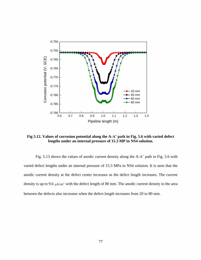
77

0.6 0.7 0.8 0.9 1.0 1.1 1.2 1.3 1.4-0.790

-0.785

-0.780

-0.775

-0.770

-0.765

-0.760

-0.755

-0.750C

orr

osio

n p

ote

ntia

l (V

, S

CE

)

20 mm

40 mm

60 mm

80 mm

Pipeline length (m)

Fig 5.12. Values of corrosion potential along the A-A’ path in Fig. 5.6 with varied defect


Fig. 5.13 shows the values of anodic current density along the A-A’ path in Fig. 5.6 with

varied defect lengths under an internal pressure of 15.3 MPa in NS4 solution. It is seen that the

anodic current density at the defect center increases as the defect length increases. The current

density is up to 9.6 2μA/cm with the defect length of 80 mm. The anodic current density in the area

between the defects also increases when the defect length increases from 20 to 80 mm.

78

0.6 0.7 0.8 0.9 1.0 1.1 1.2 1.3 1.44

5

6

7

8

9

10 20 mm

40 mm

60 mm

80 mm

An

odic

cu

rren

t d

en

sity (

A/c

m2)

Pipeline length (m)

Fig 5.13. Values of anodic current density along the A-A’ path in Fig. 5.6 with varied defect


5.4 Maximum spacing between corrosion defects for their mutual interaction

The modeling results in this work show that, depending on the spacing between the

longitudinally aligned corrosion defects, the mutual interaction exists to affect not only the local

stress/strain distribution, but also the electrochemical corrosion properties. When the defect

spacing is 150 mm, the anodic current density in the area between the defects is identical to that

of the uncorroded area, as seen in Fig. 5.9. Once the spacing decreases to 100 mm, the anodic

current density increases apparently. At the spacing of 5 mm, the anodic current densities at the

defect center and the adjacent area are close each other. Therefore, a critical longitudinal spacing

79

exists, below which there is an interaction between the corrosion defects to enhance the corrosion

rate. From this work, this value is between 100 mm and 150 mm. To determine the critical spacing

between corrosion defects, the anodic current density of one end at the A-A’ path in Fig. 5.6 (i.e.,

ZA-A’= 0 m) is used as a reference. The criterion used to evaluate the interaction between adjacent

corrosion defects is defined as

( )

( )

( )

( )

A-A

A-A

A-A

A-A

Anodic current density Z =0 m1

Anodic current density Z =1 m

Anodic current density Z =0 m1

Anodic current density Z =1 m

interaction.

no interaction.

，

，

(5.1)

As the 3-D model is established symmetrically relative to z = 1 m surface, the anodic current

density at this surface refers to that at the area between the corrosion defects. When the ratio

defined in Eq. (5.1) is greater or equal to 1, there is no interaction between the corrosion defects.

If the ratio is smaller than 1, an interaction exists between the defects. The smaller the ratio, the

more significant the effect of interaction between corrosion defects on anodic current density of

the steel in the aqueous solution.

Fig. 5.14 shows the maximum spacing between adjacent corrosion defects to enable an

interaction between the defects as a function of the defect length. It is seen that the maximum

interacting spacing between corrosion defects increases as the defect length increases. For short

defects such as those with a length of 20 mm, 40 mm and 60 mm, the maximum interacting spacing

increases rapidly with the defect length. When the defect length is longer than 80 mm, the increase

of the maximum interacting spacing with the defect length becomes slow. For the defect length of

80

60 mm, the maximum interacting spacing is 137.2 mm. Table 5.1 shows the maximum interacting

spacing determined by the existing codes and standards. By comparison, the maximum interacting

spacing in terms of the M-E effect in this work is close to the value derived by DNV-RF-F101

code at the defect length of 60 mm [6].

20 40 60 80 100 1200

40

80

120

160

200

240

Maxim

um

inte

racting s

pacin

g (

mm

)

Defect length (mm)

Fig 5.14. Maximum spacing between adjacent corrosion defects to enable an interaction

between the defects as a function of the defect length.

81

Table 5.1. Various rules governing interaction of multiple defects present on pipelines,

where Lim

LSis the maximum longitudinal spacing, D is the pipe diameter, t is pipe wall

thickness, L1 and L2 are lengths of corrosion defects.

Interaction rules Longitudinal limit Lim

LS Lim

LS

CW rule [5] 1 2min( , )Lim

LS L L= 60.0 mm

DNV-RP-F101 [6] 2.0Lim

LS Dt= 135.5 mm

6WT rule [7] 6Lim

LS t= 60.0 mm

3WT rule [8] 3Lim

LS t= 30.0 mm

5.5 M-E effect of adjacent corrosion defects on pipelines

This work demonstrates that an increase of the length of corrosion defect, while keeping

its depth fixed, enhances the local stress, shifts the corrosion potential negatively and increases the

anodic current density at both defect center and the area between the adjacent defects (Figs. 5.11-

13). It has been demonstrated above that the applied mechanical stress can increase the

electrochemical activity of steels in aqueous environments, causing a negative shift of equilibrium

potential. Due to the increasing stress concentration, the corrosion potential at the defect would

increase negatively with the increasing defect length. As shown in Figs. 5.11 and 5.13, when the

corrosion defects are relatively short, e.g., 20 mm, the difference of corrosion potentials at the

corrosion defect and the uncorroded area is slight, approximately 6 mV. As the corrosion defects

are as long as 80 mm, the potential difference increases to 28 mV, with the most negative potential

at the central bottom of the defects due to the highest local stress. Furthermore, the group’s

previous work [32] demonstrated that the region on a steel with a high stress, e.g., the defect center,

serves as anode, and the region with a low stress, e.g., the mouth of corrosion defects, serves as

82

cathode. The presence of corrosion defects on the steel is actually composed of a number of local

galvanic cells. The anodic dissolution rate at the defect center is enhanced by the high stress/strain

concentration. In this work, as the defect length increases, the defect center is associated with a

high von Mises stress, while the stress on the defect mouth lowers. The difference in local stress

distribution at the corrosion defects results in an increased anodic current density at the defect

center.

The spacing between adjacent corrosion defects is an important parameter affecting M-E

effect. In this work, the influence of the defect spacing on M-E effect was investigated under two

stressing conditions, i.e., an axial loading and an internal pressure on the pipe to generate a hoop

stress, by 2-D and 3-D models, respectively. There are different results observed, as shown in Figs.

5.1 and 5.5. As the defect spacing reduces, there is a strong interaction between the corrosion

defects, resulting in a high plastic stress between the defects under the hoop stress condition (Fig.

5.5). However, the area is still in an elastic stress state at the identical spacing under the axial

loading (Fig. 5.1). When a pipeline is under an axial loading, i.e., a uniaxial stress state, the

additional bending moment caused by the geometrical deformation is negligible. Thus, the stress

between two adjacent corrosion defects is small. For pipelines with a hoop stress along the

circumferential direction, the radial displacement of corrosion defects is larger than that of the

uncorroded region, resulting in an additional bending moment. Therefore, the local stress at the

defects and the area between the defects is increased remarkably.

The different stress status under the axial stress and the hoop stress result in different

distributions of corrosion potential and anodic current density, as seen in Figs. 5.3, 5.4, 5.9 and

5.10. Under the axial loading, the corrosion potential at the defects drops negatively by about 2

mV only (Fig. 5.3), which is almost negligible, when the defect spacing reduces from 150 mm to

83

5 mm. The anodic current density at the defects remains unchanged (Fig. 5.4). However, under a

hoop stress condition, the corrosion potential shifts negatively by about 27 mV with the same

reduction of the defect spacing (Fig. 5.10). Correspondingly, the anodic current density increases

by 4.9 µA/cm2 in the area between the adjacent corrosion defects (Fig. 5.9). The hoop stress

condition generated on the pressurized pipeline drives an enhanced M-E effect between adjacent

corrosion defects as the defect spacing reduces, while the effect of the uniaxial stress is ignorable.

5.6 Summary

A mechano-electrochemical effect exists between adjacent longitudinally aligned

corrosion defects on pipelines. The defect spacing, the stressing condition that the pipeline

experiences and the defect geometry (i.e., the defect length while its depth is fixed) are important

factors affecting the M-E effect. As the defect spacing reduces, there is a strong M-E effect

between the defects, resulting in a high plastic stress between the defects under the hoop stress

condition. However, the area is still in an elastic stress state at the identical spacing when the

pipeline is under axial loading. The hoop stress condition drives an enhanced M-E effect between

adjacent corrosion defects as the defect spacing reduces, while the effect of uniaxial stress is

ignorable.

An increase of the length of corrosion defects, while keeping the defect depth fixed,

enhances the local stress at the defects, shifts the corrosion potential negatively and increases the

anodic current density at both defect center and the area between the adjacent defects.

For multiple corrosion defects, a critical spacing exists, below which there is an interaction

between the defects to enhance the corrosion rate. The maximum interacting spacing between the

defects increases as the defect length increases.

84

Chapter Six: Investigation by numerical modeling of the mechano-electrochemical

interaction of circumferentially aligned corrosion defects on pipelines3

6.1 Modeling of stress distribution at circumferentially aligned corrosion defects on pipelines

Fig. 6.1 shows the distributions of von Mises stress at the circumferentially aligned

corrosion defects with a fixed circumferential spacing of 3.6° under varied internal pressures.

Generally, the stress level increases with the increasing internal pressure. When the internal

pressure is 16 MPa (Fig. 6.1a), the stress is evenly distributed on the pipe, except the inside edges

of the defects where the stress is slightly higher than the yielding stress. As the internal pressure

increases to 16.5 MPa, the stress concentration spreads in the defects, and the stress level increases

(Fig. 6.1b). With the further increase of the internal pressure to 17 MPa, the stress concentration

exceeds the yielding stress (Fig. 6.1c), and the defects are under plastic deformations. At the

internal pressure of 17.5 MPa and 18 MPa, the stress concentrations inside the defects close to the

ultimate tensile strength of the steel (Figs. 6.1d and 6.1e). It is interesting to see that, while the

plasticity occurs at the corrosion defects under high internal pressures, the stress at the defect

adjacent area slightly exceeds the yielding stress level. Therefore, from the viewpoint of

mechanical stress field, the increasing internal pressure results in local stress concentration and

plasticity occurring primarily at the corrosion defects. There is only slight effect on the adjacent

area between the defects.


Jialin Sun, Y. Frank Cheng, Investigation by numerical modeling of the mechano-electrochemical interaction of

circumferentially aligned corrosion defects on pipelines, Thin-Walled Structures 144 (2019) 106314/1-11.

85

c) 17 MPa

a) 16 MPa

b) 16.5 MPa

86


with a fixed circumferential spacing of 3.6° under varied internal pressures.

Fig. 6.2 shows the distributions of von Mises stress at the circumferentially aligned

corrosion defects with varied circumferential spacings under a fixed internal pressure of 18 MPa.

It is seen that, when the circumferential spacing of the two defect is 1.8°, the maximum stress

concentration occurs at the edges of the defects, as indicated by the dark red color. The adjacent

d) 17.5 MPa

e) 18 MPa

87

area between the defects also has a high stress concentration, as colored in light blue (Fig. 6.2a),

and the stress level exceeds the yielding stress. At the circumferential spacing of 10.8°, the stress

distribution inside the defects is identical to that in Fig. 6.2a, but the stress concentration at the

adjacent area reduces to elastic range (Fig. 6.2b). This phenomenon is also found in Figs. 6.2c and

6.2d, where the circumferential spacing of the defects increases to 21.6° and 36°, respectively.

Therefore, when the defect spacing is sufficiently small, such as 1.8° in this work, the adjacent

area between the defects is under stress concentration to generate a plastic zone. With the increase

of the defect spacing circumferentially, the interaction between the defects disappear, and the

defects can be treated separately.

a) 1.8o

b) 10.8o

88


with varied circumferential spacings under a fixed internal pressure of 18 MPa.

6.2 Modeling of corrosion potential at circumferentially aligned corrosion defects on

pipelines

Fig. 6.3 shows the distributions of corrosion potential of the pipeline containing two

corrosion defects with a fixed circumferential spacing of 3.6° in the solution as a function of the

internal pressure. It is seen that, at the internal pressure of 16 MPa, an uneven potential field

initiates around the individual defects, as shown in Fig. 6.3a, where the potential at the defects is

about 10 mV more negative than other area. As the internal pressure increases to 16.5 MPa, the

potential fields of the two corrosion defects merge, with the most negative potential of about -

0.775 V (SCE) locating at the defect center (Fig. 6.3b). With the further increase of the internal

c) 21.6o

d) 36o

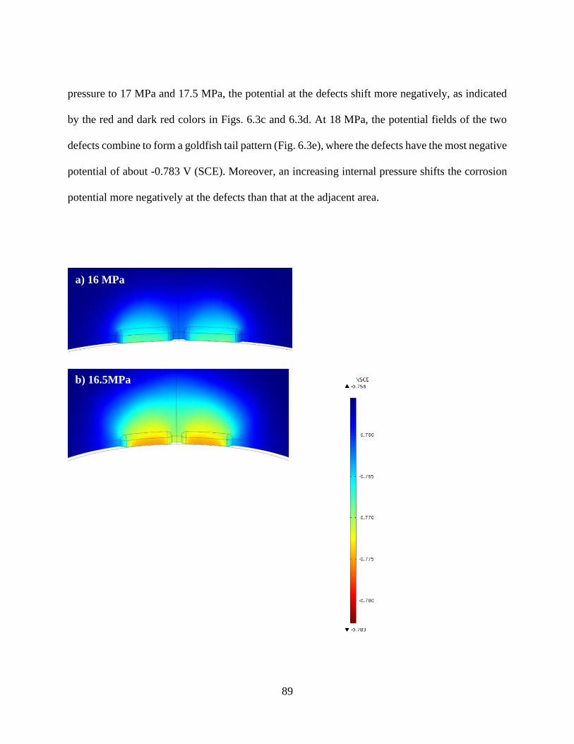
89

pressure to 17 MPa and 17.5 MPa, the potential at the defects shift more negatively, as indicated

by the red and dark red colors in Figs. 6.3c and 6.3d. At 18 MPa, the potential fields of the two

defects combine to form a goldfish tail pattern (Fig. 6.3e), where the defects have the most negative

potential of about -0.783 V (SCE). Moreover, an increasing internal pressure shifts the corrosion

potential more negatively at the defects than that at the adjacent area.

a) 16 MPa

b) 16.5MPa

90


with a fixed circumferential spacing of 3.6° in NS4 solution as a function of the internal

pressure.

Fig. 6.4 shows the distributions of corrosion potential of the pipeline containing two

corrosion defects with a fixed internal pressure of 18 MPa in NS4 solution as a function of the

circumferential spacing. It is seen that, as the spacing between corrosion defects increases, the

potential field developed on the two defects changes into two separated potential fields, each of

which is shaped of the goldfish tail pattern. Moreover, while the potential at the defects change

slightly with the increasing circumferential spacing from 1.8° to 36°, the potential in the adjacent

area between the defects shift much less negatively.

c) 17 MPa

d) 17.5 MPa

e) 18 MPa

91


with a fixed internal pressure of 18 MPa in NS4 solution as a function of the

circumferential spacing.

a) 1.8 °

b) 10.8 °

c) 21.6°

d) 36°

92

6.3 Modeling of anodic current density at circumferentially aligned corrosion defects on

pipelines

Fig. 6.5 shows the distributions of anodic current density of the pipeline containing two

corrosion defects with a fixed circumferential spacing of 3.6° in NS4 solution as a function of the

internal pressure. It is seen that, as the internal pressure increases, the anodic current density

increases, especially at the corrosion defects. At 16 MPa, while the anodic current density at the

uncorroded region is about 4.0 2μA/cm (0.05 mm/year) the defects have the anodic current density

of about 7.0 2μA/cm (0.08 mm/year) with the defect edges reaching to 9.0 2μA/cm (0.11 mm/year)

as shown in Fig. 6.5a. When the internal pressure increases to 16.5 MPa and 17 MPa, the anodic

current densities at the corrosion defects increase to 9.0 and 11.0 2μA/cm (0.13 mm/year)

respectively. With the internal pressure further increasing to 17.5 MPa and 18 MPa, the anodic

current density further increases. Particularly, the current density at the corrosion defects is up to

14.0 2μA/cm (0.16 mm/year) under the internal pressure of 18 MPa, which is over three times of

that of uncorroded region on pipelines.

a) 16 MPa

b) 16.5 MPa

93


defects with a fixed circumferential spacing of 3.6° in NS4 solution as a function of the

internal pressure.

c) 17 MPa

d) 17.5 MPa

e) 18 MPa

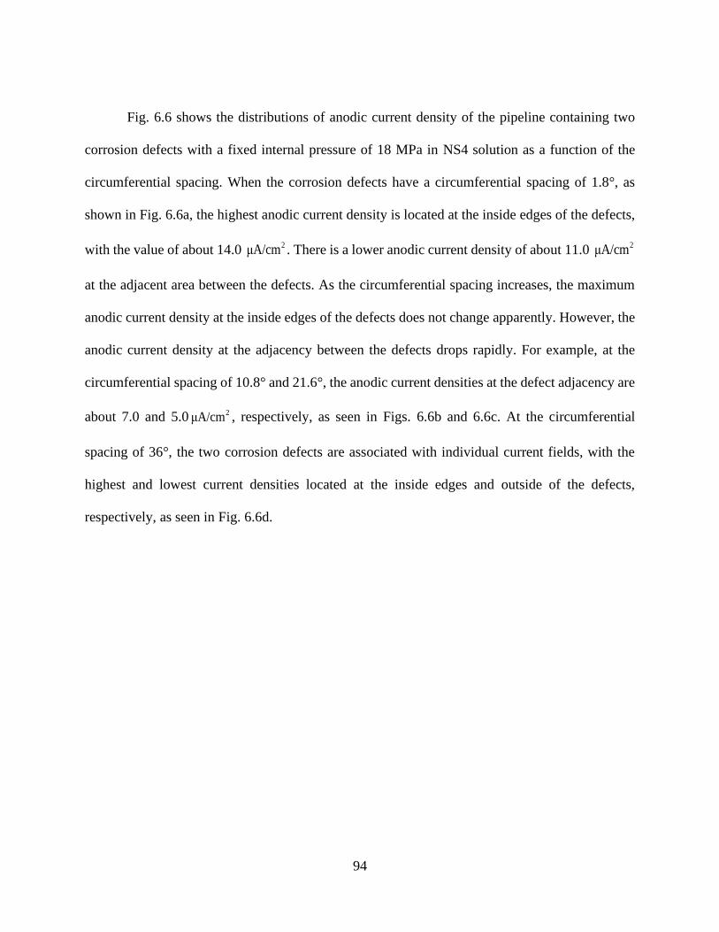
94

Fig. 6.6 shows the distributions of anodic current density of the pipeline containing two

corrosion defects with a fixed internal pressure of 18 MPa in NS4 solution as a function of the

circumferential spacing. When the corrosion defects have a circumferential spacing of 1.8°, as

shown in Fig. 6.6a, the highest anodic current density is located at the inside edges of the defects,

with the value of about 14.0 2μA/cm . There is a lower anodic current density of about 11.0

2μA/cm

at the adjacent area between the defects. As the circumferential spacing increases, the maximum

anodic current density at the inside edges of the defects does not change apparently. However, the

anodic current density at the adjacency between the defects drops rapidly. For example, at the

circumferential spacing of 10.8° and 21.6°, the anodic current densities at the defect adjacency are

about 7.0 and 5.0 2μA/cm , respectively, as seen in Figs. 6.6b and 6.6c. At the circumferential

spacing of 36°, the two corrosion defects are associated with individual current fields, with the

highest and lowest current densities located at the inside edges and outside of the defects,

respectively, as seen in Fig. 6.6d.

95

c) 21.6°

b) 10.8°

a) 1.8°

96


defects with a fixed internal pressure of 18 MPa in NS4 solution as a function of the


6.4 Analysis of stress, corrosion potential and anodic current density at circumferentially

aligned corrosion defects on pipelines

The numerical modeling results show that, for pressurized pipelines containing

circumferentially aligned corrosion defects, the maximum von Mises stress, the most negative

corrosion potential and the highest anodic current density occur at the corrosion defects,

particularly, the inside edges and the defect center. Further analysis is conducted on von Mises

stress, corrosion potential and anodic current density along the corrosion defects. Figs. 6.7-6.9

show the values of von Mises stress, corrosion potential and anodic current density, respectively,

on two circumferential aligned corrosion defects on pipeline under internal pressure of 18 MPa

and varied circumferential spacings. For the stress distributions in Fig. 6.7, the local stress at the

adjacent area between the defects (i.e., 449.07 MPa) is higher than the stress of the uncorroded

region. When the circumferential spacing is sufficiently large, there is no stress concentration at

the defect adjacency.

d) 36°

97

0.0 0.1 0.2 0.3 0.4 0.5 0.6 0.7300

350

400

450

500

550

600

650

Von

Mis

es s

tres

s (M

Pa

)

1.8o

10.8o

21.6o

36o

Arc length

Fig 6.7. Values of von Mises stress on two circumferential aligned corrosion defects on

pipeline under internal pressure of 18 MPa and varied circumferential spacings.

For the corrosion potential distribution in Fig. 6.8, generally, there is the most negative

corrosion potential at the defect center. As the circumferential spacing between the defects reduces,

the corrosion potential at the defect adjacency shifts more negatively, but there is no apparent

effect on the potential at the defect center. When the defect spacing exceeds 21.6°, the corrosion

potential at the defect adjacency becomes independent of the circumferential spacing. Moreover,

the difference of corrosion potentials of outside and inside the defects is over 10 mV (SCE).

98

0.0 0.1 0.2 0.3 0.4 0.5 0.6 0.7-0.775

-0.770

-0.765

-0.760

-0.755

-0.750

Co

rro

sio

n p

ote

nti

al

(V, S

CE

)

1.8o

10.8o

21.6o

36o

Arc length

Fig 6.8. Values of corrosion potential on two circumferential aligned corrosion defects on

pipeline under internal pressure of 18 MPa and varied circumferential spacings.

For the anodic current density distribution in Fig. 6.9, there are the highest and lowest

anodic current densities at the inside defects and outside edges, respectively. At small

circumferential spacing such as 1.8°, the anodic current density at the defect adjacency is higher

than that of uncorroded region.

99

0.0 0.1 0.2 0.3 0.4 0.5 0.6 0.7 0.8

3

4

5

6

7

8

9

10

Anodic

curr

ent density (

A/c

m2)

1.8o

10.8o

21.6o

36o

Arc length

Fig 6.9. Values of anodic current density on two circumferential aligned corrosion defects

on pipeline under internal pressure of 18 MPa and varied circumferential spacing.

6.5 Maximum circumferential spacing of corrosion defects enabling mutual interaction

As demonstrated above, for pipelines containing multiple, circumferentially aligned

corrosion defects, a M-E effect exists between the defects when their spacing is within a certain

range. The M-E effect would result in a high local stress concentration, negative corrosion

potential and a large anodic current density at the defect adjacency, all of which contribute to an

increased local corrosion of the pipeline steel in service environments. Furthermore, the degrees

of the interaction from electrochemical field and mechanical stress field are different. For example,

when the circumferential spacing is up to 21.6°, the von Mises stress at the defect adjacency

decreases to the same level as that of the uncorroded region, as shown in Figs. 6.2 and 6.7. This is

100

defined as non-interacting defects from the mechanical stress perspective. However, the anodic

current density at the adjacent area is still 25 % lower than that of the uncorroded region at the

same circumferential spacing (Fig. 6.9), indicating that the interaction still exists between the

corrosion defects in the electrochemical corrosion field. Therefore, selection of a proper criterion

to evaluate the interaction between adjacent corrosion defects is critical for defect assessment on

pipelines.

In this work, a new approach is proposed to define the separation of adjacent corrosion

defects which can be considered as non-interacting. The approach is similar to that used in

maximum circumferential interacting spacing (MCIS) assessment [67], and defined as the ratio

(A) of the anodic current density at the middle of the defect adjacency to that of the uncorroded

region

anodic current density at the middle of the spacing between adjacent defects

anodic current density at uncorroded region

if 1, interaction

if =1, no interaction

A

A

A

=

(6.1)

The adjacent corrosion defects can interact to result in a local anodic current density larger than

that of the uncorroded region. The larger the ratio A, the stronger the interaction exists between

the adjacent defects. When A is equal to 1, the anodic current density at the defect adjacency is

same as that of the uncorroded region, where there is no mutual interaction between the two

corrosion defects. The defects can thus be dealt with as the individual single defects.

101

The approach is used to determine the MCIS between adjacent corrosion defects in this

work. An examination of the numerical results in Fig. 6.9 shows that, under a given internal

pressure, two circumferentially aligned defects have interactions in both the mechanical stress and

electrochemical corrosion fields, especially at small circumferential spacing of 1.8°. As MCIS can

be influenced by defect geometry, the geometrical parameters, i.e., defect width (w), defect length

(l), defect depth (d) and the circumferential spacing, are normalized as non-dimensional by

converting them to be related to the pipeline geometry including the pipe diameter (D) and pipe

wall thickness (t). For simulation, defects with a circumferential width of 8° (0.025πD), 16°

(0.05πD) and 32° (0.1πD) are used to represent the narrow, normal and wide defects, respectively,

with the three groups of defects with the same length of Dt and depth of 0.7t. Fig. 6.10 shows

the ratio of the anodic current densities at the defect adjacency to that of the uncorroded region as

a function of the dimensionless circumferential spacing SC/πD for defect of 0.05πD in width. It is

seen that the ratio decreases with the increasing SC/πD, indicating that the interaction between the

corrosion defects reduces with the increase of the circumferential spacing. When the

circumferential spacing reaches 0.08πD, the ratio A approaches 1, where the adjacent corrosion

defects can be treated as two single isolated defects at this spacing when the internal pressure is

18 MPa.

102

-0.02 0.00 0.02 0.04 0.06 0.08 0.10 0.120.8

1.0

1.2

1.4

1.6

1.8

2.0

2.2

A(A

nod

ic c

urr

ent

de

nsity r

atio

)

SC /D



defect of 0.05πD in width.

For defects of 0.025πD and 0.1πD in width, the ratio of the anodic current densities at the

defect adjacency to that at the uncorroded region as a function of the dimensionless circumferential

spacing SC/πD are shown in Figs. 6.11 and 6.12, respectively. As expected, the ratio A decreases

as the SC/πD increases. For the narrow defects, the critical spacing is 0.07πD, beyond which there

is no interaction between the defects (Fig. 6.11). However, for the wide defects, the critical spacing

is also about 0.08πD, (Fig. 6.12). The results indicate that, after exceeding a certain value, the

defect width does not influence the degree of interaction between two circumferentially aligned

corrosion defects.

103

-0.02 0.00 0.02 0.04 0.06 0.08 0.10 0.120.8

1.0

1.2

1.4

1.6

1.8

2.0

2.2

A(A

nodic

curr

ent density r

atio)

SC /D




-0.02 0.00 0.02 0.04 0.06 0.08 0.10 0.120.8

1.0

1.2

1.4

1.6

1.8

2.0

2.2

A(A

nod

ic c

urr

ent

de

nsity r

atio

)

SC /D




104

6.6 Summary

A finite element based multi-physics field coupling model is developed to investigate the

mechano-electrochemical (M-E) effect between adjacent, circumferentially aligned corrosion

defects on X46 steel pipeline. A M-E effect exists between the defects when their spacing is within

a certain range. The M-E effect results in a high local stress concentration, negative corrosion

potential and a large anodic current density at the defect adjacency, all of which contribute to an

increased local corrosion of the pipeline steel in service environments. The degrees of the

interaction from electrochemical corrosion field and the mechanical stress field are different.

Mechanically, the increasing internal pressure results in local stress concentration and

plasticity occurring primarily at the corrosion defects, while the effect on the adjacent area between

the defects is slight at individual circumferential spacing. When the defect spacing is sufficiently

small, such as 1.8° in this work, the defect adjacency is under stress concentration to generate a

plastic zone. With the increase of the defect spacing circumferentially, the interaction between the

defects disappears, and the defects can be treated separately.

Electrochemically, an increasing internal pressure results in shift of corrosion potential

more negatively and more rapid increase of anodic current density at the corrosion defects than

those at the adjacent area between the defects at individual circumferential spacing. While the

potential and anodic current density at the defects change slightly with the increasing

circumferential spacing from 1.8° and 36°, those at the defect adjacency shift much less negatively

and reduce more rapidly, respectively.

The ratio of the anodic current density at the middle of the defect adjacency to that of the

uncorroded region is proposed to define the separation of adjacent corrosion defects which can be

considered as non-interacting. The critical ratio depends on defect geometry (such as the defect

105

width as studied in this work) under a given internal pressure. For example, for corrosion defects

with 0.025πD, 0.05πD and 0.1πD in width on pipeline under an internal pressure of 18 MPa, the

critical spacing are 0.07πD, 0.08πD and 0.08πD, respectively, beyond which there is no interaction

between the defects.

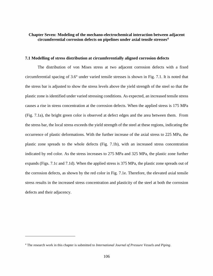
106

Chapter Seven: Modeling of the mechano-electrochemical interaction between adjacent

circumferential corrosion defects on pipelines under axial tensile stresses4

7.1 Modelling of stress distribution at circumferentially aligned corrosion defects

The distribution of von Mises stress at two adjacent corrosion defects with a fixed

circumferential spacing of 3.6° under varied tensile stresses is shown in Fig. 7.1. It is noted that

the stress bar is adjusted to show the stress levels above the yield strength of the steel so that the

plastic zone is identified under varied stressing conditions. As expected, an increased tensile stress

causes a rise in stress concentration at the corrosion defects. When the applied stress is 175 MPa

(Fig. 7.1a), the bright green color is observed at defect edges and the area between them. From

the stress bar, the local stress exceeds the yield strength of the steel at these regions, indicating the

occurrence of plastic deformations. With the further increase of the axial stress to 225 MPa, the

plastic zone spreads to the whole defects (Fig. 7.1b), with an increased stress concentration

indicated by red color. As the stress increases to 275 MPa and 325 MPa, the plastic zone further

expands (Figs. 7.1c and 7.1d). When the applied stress is 375 MPa, the plastic zone spreads out of

the corrosion defects, as shown by the red color in Fig. 7.1e. Therefore, the elevated axial tensile

stress results in the increased stress concentration and plasticity of the steel at both the corrosion

defects and their adjacency.

4 The research work in this chapter is submitted to International Journal of Pressure Vessels and Piping.

107

a) 175 MPa

b) 225 MPa

c) 275 MPa

d) 325 MPa

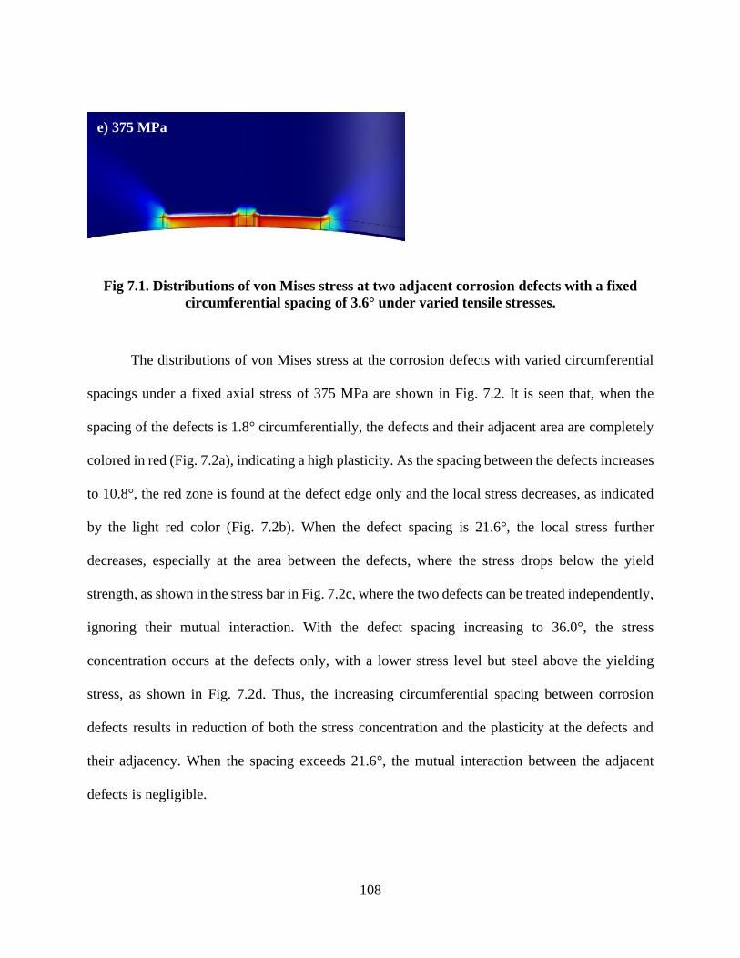
108

Fig 7.1. Distributions of von Mises stress at two adjacent corrosion defects with a fixed

circumferential spacing of 3.6° under varied tensile stresses.

The distributions of von Mises stress at the corrosion defects with varied circumferential

spacings under a fixed axial stress of 375 MPa are shown in Fig. 7.2. It is seen that, when the

spacing of the defects is 1.8° circumferentially, the defects and their adjacent area are completely

colored in red (Fig. 7.2a), indicating a high plasticity. As the spacing between the defects increases

to 10.8°, the red zone is found at the defect edge only and the local stress decreases, as indicated

by the light red color (Fig. 7.2b). When the defect spacing is 21.6°, the local stress further

decreases, especially at the area between the defects, where the stress drops below the yield

strength, as shown in the stress bar in Fig. 7.2c, where the two defects can be treated independently,

ignoring their mutual interaction. With the defect spacing increasing to 36.0°, the stress

concentration occurs at the defects only, with a lower stress level but steel above the yielding

stress, as shown in Fig. 7.2d. Thus, the increasing circumferential spacing between corrosion

defects results in reduction of both the stress concentration and the plasticity at the defects and

their adjacency. When the spacing exceeds 21.6°, the mutual interaction between the adjacent

defects is negligible.

e) 375 MPa

109

Fig 7.2. Distributions of von Mises stress at the corrosion defects with varied

circumferential spacings under a fixed axial stress of 375 MPa.

a) 1.8°

b) 10.8°

c) 21.6°

d) 36°

110

7.2 Modelling of corrosion potential at circumferentially aligned corrosion defects

Potential is a thermodynamic parameter indicating the electrochemical activity of steels in

an aqueous solution. To investigate the electrochemical activity of the corrosion defects in the

simulated NS4 solution, the distribution of corrosion potential at the defects with a fixed

circumferential spacing of 3.6° is modelled in the near-neutral pH solution as a function of the

axial tensile stress, as shown in Fig. 7.3. It is seen that, under small stresses such as 175 MPa, the

potential field on the steel surface is uniform and the potential is about -0.760 V (SCE) (Fig. 7.3a).

As the tensile stress increases to 225 MPa, a non-uniform potential field is generated around the

corrosion defects, indicated by the light blue color in Fig. 7.3b, where the local potential shifts

negatively to about -0.765 V (SCE). With the further increase of the tensile stress to 275 MPa, the

uneven potential distribution is more apparent (Fig. 7.3c), and the local potential at the defects

shifts more negatively. At 325 MPa, the potential field shaped of a butterfly is observed at the

defects (Fig. 7.3d), where the light red color indicates the local potential of about -0.775 V (SCE)

at the corrosion defects. When the tensile stress is further increased to 375 MPa, the most negative

potential of about -0.779 V (SCE) is recorded at the bottom of the corrosion defects, as shown by

the dark red color in Fig. 7.3e. The potential field outside the corrosion defects also shifts

negatively with the increasing tensile stress. Thus, as the axial tensile stress increases, the potential

of the steel shifts more negatively, with the most negative potential recorded at the defect bottom

and the adjacent area between the defects. Moreover, the negative potential zone expands with the

increasing axial stress.

111

Fig 7.3. Distributions of corrosion potential at the defects with a fixed circumferential

spacing of 3.6° in the near-neutral pH NS4 solution as a function of the axial tensile stress.

b) 225 MPa

c) 275 MPa

d) 325 MPa

a) 175 MPa

e) 375 MPa

112

Fig. 7.4 shows the distribution of corrosion potential at the corrosion defects under a fixed

tensile stress of 375 MPa in the simulated NS4 solution as a function of the circumferential

spacing. At the circumferential spacing of 3.6°, the butterfly shaped potential field is observed

(Fig, 7.4a), where the potentials at the two corrosion defects and their adjacency are about -0.779

V (SCE), which is more negative than that of other area. As the spacing angle increases, the

potential shifts less negatively. While the corrosion defects are still associated with the most

negative potential at specific circumferential spacing, the potential at the adjacent area of the

defects becomes less negatively. For example, as the circumferential spacing increases to 10.8°

and 21.6°, the potentials at the corrosion defects are about -0.776 V (SCE) and -0.772 V (SCE),

respectively, while the potentials at the adjacency of the defects are slightly less negative, i.e., -

0.775 V (SCE) and -0.770 V (SCE), respectively. When the circumferential spacing increases to

36°, the potentials at the corrosion defects and their adjacency further increase to -0.773 V (SCE)

and -0.766 V (SCE), respectively. Each corrosion defect tends to develop its own butterfly-shaped

potential zone, with the adjacent area merging together, as seen in Fig. 7.4d. Thus, under a certain

axial tensile stress, the increase in circumferential spacing between corrosion defects shifts the

corrosion potential less negatively. The effect is more apparent at the adjacent area between the

defects than that at the corrosion defects.

113

Fig 7.4. Distributions of corrosion potential at the corrosion defects under a fixed tensile

stress of 375 MPa in the simulated NS4 solution as a function of the circumferential

spacing.

a) 1.8°

b) 10.8°

c) 21.6°

d) 36°

114

7.3 Modelling of anodic current density at circumferentially aligned corrosion defects

Anodic current density is the indicator of corrosion rate of steels when measured

electrochemically. The distribution of the anodic current density at the corrosion defects with a

fixed circumferential spacing of 3.6° is modelled in the near-neutral pH NS4 solution as a function

of the axial tensile stress, as shown in Fig. 7.5. The application of a small tensile stress such as 175

MPa would not change the anodic current density at the corrosion defects, as compared to the non-

corroded area on the steel pipe (Fig. 7.5a). When the tensile stress is increased to 225 MPa and

275 MPa, the anodic current density increases primarily on the circumferential edge of the defects

and the adjacency between them, as indicated by the light green color in Figs. 7.5b and 7.5c. As

the stress further increases to 325 MPa and 375 MPa, the anodic current density over the entire

defects and the adjacent area increases greatly, as shown in red color in Figs. 7.5d and 7.5e.

Apparently, the increased tensile stress enhances the anodic current density, i.e., corrosion rate, at

the corrosion defects and the adjacent area.

Fig. 7.6 shows the distributions of anodic current density at the corrosion defects under a

fixed tensile stress of 375 MPa in the simulated NS4 solution as a function of the circumferential

spacing. As the defect spacing increases, the anodic current density decreases, as indicated by the

red color becoming lighter with the increased spacing. Moreover, at the small circumferential

spacing such as3.6°, there is a high anodic current density at the defect adjacency. The anodic

current density decreases with the circumferential spacing. It is thus seen that the anodic current

density at the corrosion defects and the adjacent area continuously decreases as the circumferential

spacing increases.

115

Fig 7.5. Distributions of anodic current density at the corrosion defects with a fixed

circumferential spacing of 3.6° in the near-neutral pH NS4 solution as a function of the

axial tensile stress.

a) 175 MPa

b) 225 MPa

c) 275 MPa

e) 375 MPa

d) 325 MPa

116

Fig 7.6. Distributions of anodic current density at the corrosion defects under a fixed tensile

stress of 375 MPa in NS4 solution as a function of the circumferential spacing.

a) 1.8°

b) 10.8°

c) 21.6°

d) 36°

117

7.4 Distributions of von Mises stress, corrosion potential and anodic current density across

the corrosion defects under varied axial tensile stresses

To further show the detail of the stress, corrosion potential and anodic current density

distributions across the corrosion defects, a mapping of the three parameters along the

circumferential curvature at the middle of the defect is conducted under an axial tensile stress of

375 MPa, and the results are shown in Figs. 7.7-7.9, respectively. Generally, the stress is

distributed symmetrical relative to the adjacent center between the defects, as marked in Fig. 7.7.

As the defects become closer, the stresses at both the defects and their adjacency increase. For

example, at the circumferential spacing of 1.8°, the von Mises stress at the adjacent center is up to

574.24 MPa, indicating that the adjacent area is under plastic deformations. Only when the

circumferential spacing is larger than 14.4°, the defect adjacency becomes elastically deformed.

The average stress level around corrosion defects reduces continuously with the increasing

circumferential spacing between the defects.

Furthermore, under specific tensile stresses, there is always the most negative corrosion

potential at the defect center, i.e., the highest thermodynamic activity. However, the potential at

the defect adjacency depends on the circumferential spacing between them. At 1.8°, there is the

most negative potential of -0.779 V (SCE) at the middle of the adjacency. As the circumferential

spacing increases, the corrosion potential shifts less negatively. At big spacing angles, the most

negative potential is recorded at the defects, rather than their adjacent area. Opposite to the

corrosion potential distribution, there is always the maximum anodic current density, i.e., the

highest corrosion rate, at the defects under specific tensile stresses. As the circumferential spacing

between the defects increases, the anodic current densities at both the defects and the adjacent area

decrease.

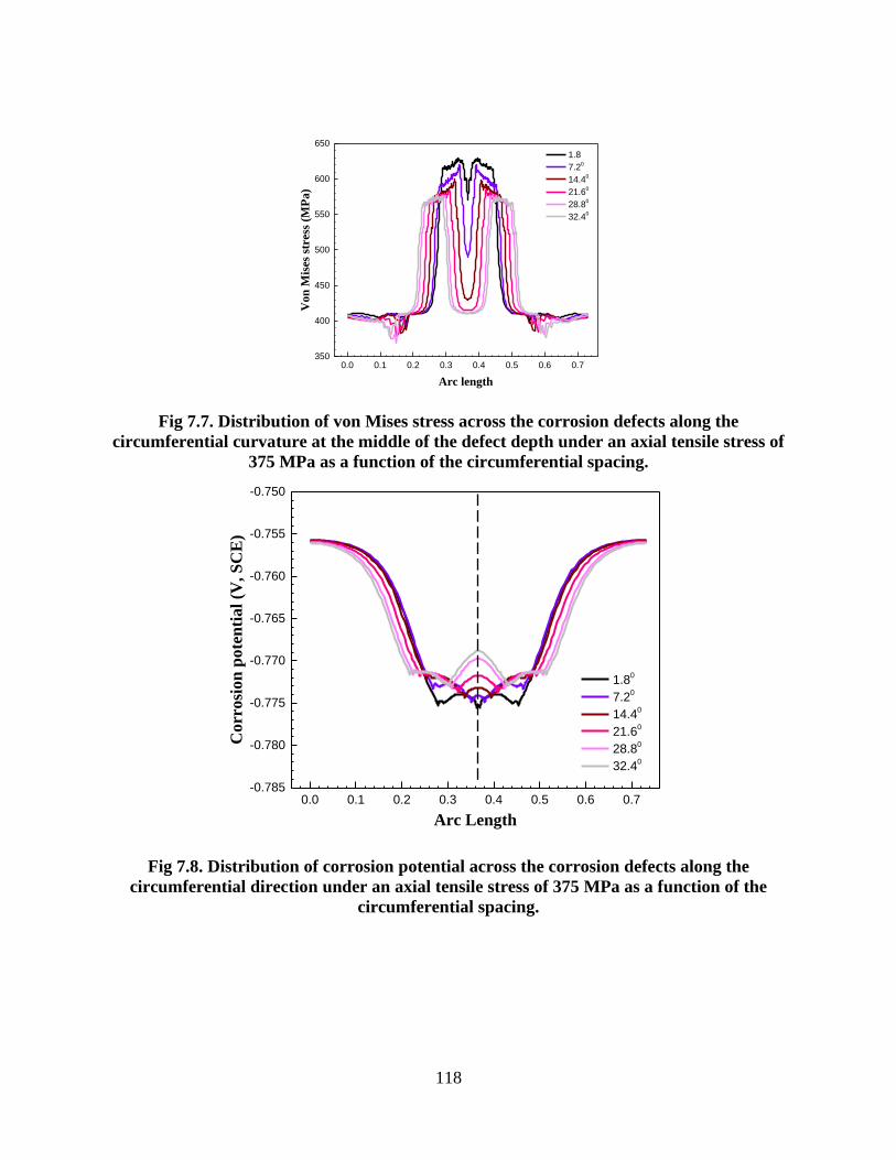
118

0.0 0.1 0.2 0.3 0.4 0.5 0.6 0.7350

400

450

500

550

600

650

1.8

7.20

14.40

21.60

28.80

32.40

Von

Mis

es s

tres

s (M

Pa)

Arc length

Fig 7.7. Distribution of von Mises stress across the corrosion defects along the

circumferential curvature at the middle of the defect depth under an axial tensile stress of

375 MPa as a function of the circumferential spacing.

0.0 0.1 0.2 0.3 0.4 0.5 0.6 0.7-0.785

-0.780

-0.775

-0.770

-0.765

-0.760

-0.755

-0.750

1.80

7.20

14.40

21.60

28.80

32.40

Corr

osi

on

po

ten

tia

l (V

, S

CE

)

Arc Length

Fig 7.8. Distribution of corrosion potential across the corrosion defects along the

circumferential direction under an axial tensile stress of 375 MPa as a function of the


119

0.0 0.1 0.2 0.3 0.4 0.5 0.6 0.7

3

4

5

6

7

8

9

10

An

od

ic c

urr

en

t d

en

sity (

A/c

m2)

1.80

7.20

14.40

21.60

28.80

32.40

Arc Length

Fig 7.9. Distribution of anodic current density across the corrosion defects along the

circumferential direction at the middle of the defect depth under an axial tensile stress of

375 MPa as a function of the circumferential spacing.

7.5 Maximum circumferential spacing enabling interaction between corrosion defects on

pipelines

Numerical analyses in this work show that an interaction exists between adjacent corrosion

defects, depending on their circumferential spacing, in terms of the distributions of stress,

corrosion potential and anodic current density. A reliable approach is required to define the

separation of adjacent corrosion defects, above which they can be considered as non-interacting.

According to modelling of the M-E interaction and the fact that the corrosion defect growth is

directly related to the anodic current density, a new criterion is proposed, which is similar to that

used in determination of the maximum circumferential interacting spacing (MCIS) [67], based on

anodic current density as the indicator

120

𝐴 =Anodic current density at the middle of the adjacency between corrosion defects

Anodic current density at the non-corrosion area

{if 𝐴 > 1, Interactingif 𝐴 =1, No interaction

(7.1)

The ratio, A, is used to determine whether the interaction exists between adjacent corrosion defects,

considering that the mutual interaction would increase the electrochemical corrosion at the defects

and the adjacent area. The larger the ratio A, the higher the andic current density at the adjacency,

and thus the stronger the mutual interaction is. When A=1, the anodic current density at the

adjacency is equal to that of the non-corroded area, indicating that the interaction does not exist

between the corrosion defects. As a result, the two defects can be analyzed separately. Generally,

the MCIS can be influenced by the defect geometry and the stressing condition. For normalization,

the defect geometries, i.e., width (w), length (l), depth (d) and the circumferential spacing, are

converted into non-dimensional variables and expressed using the pipeline geometries, i.e., the

outer diameter of pipeline (D) and the pipe wall thickness (t).

To determine the effect of circumferential spacing of corrosion defects on M-E effect, three

widths scenarios are simulated, i.e., 8° (0.025πD), 16° (0.05πD) and 32° (0.1πD), while the defect

length and depth are fixed as Dt and 70%t, respectively. Fig. 7.10 shows the ratio, A, as defined

in Equation (7.1), as a function of the dimensionless circumferential spacing, SC/πD, where Sc

refers to the length of the arc between the edges of the adjacent corrosion defects and the defect

width is 0.05πD. It is seen that the ratio A decreases with the increasing SC/πD, indicating that the

M-E effect between the adjacent corrosion defects reduces with the increasing spacing between

121

them. When the circumferential spacing reaches 0.09πD, the ratio A tends to be 1. Therefore, the

adjacent corrosion defects would not generate mutual interaction and can be regarded as two

isolated defects when their spacing exceeds 0.09πD.

-0.02 0.00 0.02 0.04 0.06 0.08 0.10 0.120.8

1.0

1.2

1.4

1.6

1.8

2.0

A(A

nodic

curr

ent density r

atio)

SC /D

Fig 7.10. The ratio, A as a function of the dimensionless circumferential spacing, SC/πD,

while the defect length, depth and width are Dt , 70%t and 0.05πD, respectively. Sc refers

to the length of the arc between the edges of the adjacent corrosion defects.

The influence of the circumferential spacing between corrosion defects with the width of

0.025πD on the anodic current density at the defect adjacency is shown in Fig. 7.11. It is seen that

the ratio A approaches to 1 as the spacing exceeds 0.08πD. Therefore, the critical circumferential

spacing is determined to be 0.08πD for the defects with a width of 0.025πD. Fig. 7.12 shows the

relationship between the ratio A and the circumferential spacing, where the defect width is 0.1πD.

There is the same trend as those in Figs. 7.10 and 7.11. After the circumferential spacing exceeds

122

0.09πD, the ratio A becomes unity, where the mutual interaction of the adjacent corrosion defects

is negligible.

-0.02 0.00 0.02 0.04 0.06 0.08 0.10 0.120.8

1.0

1.2

1.4

1.6

1.8

2.0

A(A

nodic

curr

ent density r

atio)

SC /D

Fig 7.11. Influence of the circumferential spacing between corrosion defects on the anodic

current density at the adjacency, where the defect width is 0.025πD.

123

-0.02 0.00 0.02 0.04 0.06 0.08 0.10 0.120.8

1.0

1.2

1.4

1.6

1.8

2.0

2.2

A(A

nodic

curr

ent density r

atio)

SC /D

Fig 7.12. Relationship between the ratio A and the circumferential spacing, where the

defect width is 0.1πD.

While the numerical modelling detects the mutual interaction between adjacent corrosion

defects, this work proposes a new criterion, i.e., the ratio of the anodic current density at the defect

adjacency to that at the non-corrosion area, to evaluate the critical circumferential spacing between

the defects, above which the mutual interaction does not exist. The physical meaning of the

criterion is based on the fact that, in addition to corrosion defects, the adjacency between them

also suffers from increased anodic current density (i.e., corrosion rate) and stress concentration, as

compared to the non-corrosion area, due to the mutual interaction between the defects. This would

further reduce the failure pressure of pipelines containing multiple corrosion defects which are in

mutual interaction, compared to the pipelines containing the same number of corrosion defects that

can be treated independently. The introduction of anodic current density, rather than conventional

stress-based criteria, in defect assessment is associated with the stress-enhanced corrosion (anodic

124

current density) at both the corrosion defects and their adjacency. The main advantage of the

anodic current density criterion over a stress-based criterion is the capability of the quantitative

determination and prediction of the defect growth rate due to the stress-corrosion synergism. The

industry is thus able to estimate the remaining service life of pipelines under the given condition.

This work establishes that the mutual interaction between adjacent corrosion defects results

in the corrosion acceleration at the defects and their adjacency, as compared to the corrosion

occurring individually. Verification of the findings would be the direct comparison of the

modelling results with the actual defect growth over a time period as detected by periodic in-line

inspection. The developed model serves as a methodology to accurately predict the M-E effect of

adjacent corrosion defects and the effect on defect growth. Presently, the existing interaction rules

for evaluation of the multiple corrosion defects on pipelines ignore the stress-corrosion interaction.

Thus, the predicted failure pressure and the defect growth rate are not accurately representative of

the reality of the pipelines in the field.

7.6 Summary

The FE-based model developed in this work is able to predict the synergism of stress and

corrosion reaction at the defect area, determining the distributions of von Mises stress, corrosion

potential and anodic current density. The mutual interaction between corrosion defects under an

axial stress exists within a certain circumferential spacing between them, accelerating corrosion at

the defects and their adjacency due to the M-E coupling effect. The existence of the M-E effect is

dependent on the spacing of the adjacent corrosion defects. Generally, as the circumferential

spacing between the corrosion defects decreases, both the stress concentration and the plasticity

increase, the corrosion potential shifts more negatively and the anodic current densities at the

125

defects and their adjacency increase.

A new criterion is proposed to determine whether the mutual interaction exists between

adjacent corrosion defects based on the anodic current density at the defect adjacency relative to

that of the non-corrosion region. Under the given condition, for the corrosion defects with the

widths of 0.025πD, 0.05πD and 0.1πD (where D is the outer diameter of pipelines), the critical

spacings between adjacent, circumferentially aligned corrosion defects are 0.08πD, 0.09πD and

0.09πD, respectively, above which the mutual interaction of the adjacent corrosion defects is

negligible.

126

Chapter Eight: Modeling of mechano-electrochemical interaction at overlapped

corrosion defects and the implication on pipeline failure prediction5

8.1 Modelling of stress and anodic current density at the overlapped corrosion defects under

varied internal pressures

A 3D view of the von Mises stress distributions at the overlapped corrosion defects and on

the steel pipe under varied internal pressures is shown in Fig. 8.1. Generally, an elevated internal

pressure results in increase of the overall stress level at the defects. When the internal pressure is

11.65 MPa (Fig. 8.1a), the corrosion defects are almost in the same color as the pipe body, except

the corner and base of the bottom defect, which is colored in light blue, suggesting that the local

stress slightly exceeds the yield stress according to the stress-color bar. As the internal pressure

increases to 13.65 MPa (Fig. 8.1b), the light blue color spreads in the bottom defect with a high

stress concentration which is more apparent at the corner, but the top defect remains at the stress

level below the yield stress. With the increase of internal pressure to 15.65 MPa (Fig. 8.1c), the

local stress at the corner of the bottom defect is close to the ultimate tensile strength of the steel,

as shown by the red color, and the high stress area expands to the top defect. It is interesting to

observe that the stress level at the top defect is still below the yield stress, except its corner. When

the internal pressure further increases to 17.65 MPa, the local stress at the bottom defect is

significantly higher than the yielding stress, with the maximum stress of about 620 MPa at the

corner and edge. The stress level at the top defect also exceeds the yield stress, as seen in Fig. 8.1d.


Jialin Sun, Y. Frank Cheng, Modelling of mechano-electrochemical interaction at overlapped corrosion defects and

the implication on pipeline failure prediction, Engineering Structures, 213 (2020) 110466/1-15.

127

Thus, in the mechanical stress field, the local stress concentration increases with the internal

pressure. The bottom corrosion defect suffers from a higher stress than the top defect.

a) 11.65 MPa

b) 13.65 MPa

c) 15.65 MPa

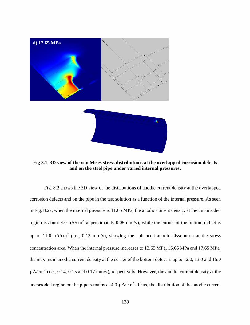
128

Fig 8.1. 3D view of the von Mises stress distributions at the overlapped corrosion defects

and on the steel pipe under varied internal pressures.

Fig. 8.2 shows the 3D view of the distributions of anodic current density at the overlapped

corrosion defects and on the pipe in the test solution as a function of the internal pressure. As seen

in Fig. 8.2a, when the internal pressure is 11.65 MPa, the anodic current density at the uncorroded

region is about 4.0 2μA/cm (approximately 0.05 mm/y), while the corner of the bottom defect is

up to 11.0 2μA/cm (i.e., 0.13 mm/y), showing the enhanced anodic dissolution at the stress

concentration area. When the internal pressure increases to 13.65 MPa, 15.65 MPa and 17.65 MPa,

the maximum anodic current density at the corner of the bottom defect is up to 12.0, 13.0 and 15.0

2μA/cm (i.e., 0.14, 0.15 and 0.17 mm/y), respectively. However, the anodic current density at the

uncorroded region on the pipe remains at 4.0 2μA/cm . Thus, the distribution of the anodic current

d) 17.65 MPa

129

density follows the similar pattern to that of the stress field, i.e., a high anodic current density is

always associated with the high stress concentration. Since the anodic current density is

proportional to the corrosion rate of the steel, a high stress concentration accelerates the local

corrosion. Particularly, at the corner of the bottom defect, the corrosion rate is approximately three

times of that of the uncorroded region on the pipe.

a) 11.65 MPa

b) 13.65 MPa

130

Fig 8.2. 3D view of the distributions of anodic current density at the overlapped corrosion

defects and on the pipe in the test solution as a function of the internal pressure.

8.2 Modelling of stress and anodic current density distributions at the overlapped

corrosion defects with varied lengths of the top layer defect

The distributions of von Mises stress at the overlapped corrosion defects with varied

lengths of the top layer defect under the fixed length of the bottom layer defect of 0.5l (i.e., 33.87

mm) and the internal pressure of 17.65 MPa are shown in Fig. 8.3. It is seen that, when the length

of the top layer defect (L1) is 0.75l (l = 67.74 mm), a slight stress concentration occurs at the

longitudinal edge of the bottom layer defect, as indicated by the light blue color, while the other

area is stressed evenly (Fig. 8.3a). As the L1 increases to l, the stress at the corner of the bottom

defect increases, while the stress at the top layer defect is still below the yield stress, as shown in

Fig. 8.3b. When L1 is increased to 1.5l, the stress at the longitudinal edge of the bottom defect

c) 15.65 MPa

d) 17.65 MPa

131

reaches the ultimate tensile stress, and the higher stress zone spreads to the top layer defect. At the

same time, a stress larger than the yield stress occurs at the corner of the top defect (Fig. 8.3c).

When L1 is equal to 2l, the stress concentration at the top layer defect expands along the

longitudinal edge, with the maximum stress observed at the bottom defect (Fig. 8.3d). Obviously,

an increase of the length of the top layer corrosion defect results in an increased stress level at the

overlapped corrosion defects, and the effect is more apparent at the bottom layer defect.

a) L1=0.75l, L2=0.5l

b) L1=l, L2=0.5l

132


lengths of the top layer defect under the fixed length of the bottom layer defect of 0.5l (i.e.,

33.87 mm) and the internal pressure of 17.65 MPa.

The distributions of the anodic current density at the overlapped corrosion defects with

varied lengths of the top layer defect under the fixed length of the bottom layer defect of 0.5l (i.e.,

33.87 mm) and the internal pressure of 17.65 MPa are shown in Fig. 8.4. Generally, as the length

of the top layer defect increases from 0.75l to 2l, the anodic current density level at the defects

increases. The maximum anodic current density is recorded at the corner of the bottom layer defect.

While the anodic current density at the uncorroded region is 4.0 2μA/cm , the highest anodic

current density of about 15.0 2μA/cm is observed at the corner of the bottom defect when the

length of the top layer defect is 2l, indicating the M-E effect on the local corrosion.

c) L1=1.5l, L2=0.5l

d) L1=2l, L2=0.5l

133

a) L1=0.75l, L2=0.5l

b) L1=l, L2=0.5l

c) L1=1.5l, L2=0.5l

134


varied lengths of the top layer defect under the fixed length of the bottom layer defect of

0.5l (i.e., 33.87 mm) and the internal pressure of 17.65 MPa.


corrosion defects with varied lengths of the bottom layer defect

The distributions of von Mises stress at the overlapped corrosion defects with varied

lengths of the bottom layer defect under the fixed length of the top layer defect of 2l (i.e., 135.48

mm) and the internal pressure of 17.65 MPa are shown in Fig. 8.5. It is seen that the stress

distribution at the bottom defect varies greatly with the increased length of the defect, but there is

little effect on the stress distribution at the top defect. It is interesting to note that, when the bottom

defect is narrow, e.g., L2 = 0.25l, a plastic zone is formed at the bottom defect, as indicated by the

yellow color in Fig. 8.5a. As the bottom defect becomes longer, a higher stress concentration is

generated primarily at the corner of the bottom defect (Figs. 8.5b-8.5d). When the length of the

bottom defect is up to 1.5l, a high stress concentration, which is close to the ultimate tensile

strength of the steel, is found at the corner of the bottom defect, while the stress at the top defect

increases slightly (Fig. 8.5d). Thus, an increase in the length of the bottom layer defect would

result in a stress concentration generated at the bottom defect primarily. The effect on the top

defect is slight.

d) L1=2l, L2=0.5l

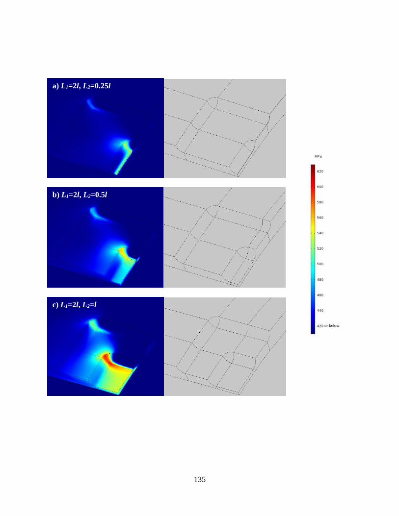
135

a) L1=2l, L2=0.25l

b) L1=2l, L2=0.5l

c) L1=2l, L2=l

136


lengths of the bottom layer defect under the fixed length of the top layer defect of 2l (i.e.,

135.48 mm) and the internal pressure of 17.65 MPa.

Fig. 8.6 shows the distributions of anodic current density at the overlapped corrosion

defects with varied lengths of the bottom layer defect under the fixed length of the top layer defect

of 2l (i.e., 135.48 mm) and the internal pressure of 17.65 MPa. Same as the stress distribution in

Fig. 8.5, the anodic current density level increases as the length of the bottom defect increases,

especially at the corner of the bottom defect.

d) L1=2l, L2=1.5l

a) L1=2l, L2=0.25l

137


varied lengths of the bottom layer defect under the fixed length of the top layer defect of 2l

(i.e., 135.48 mm) and the internal pressure of 17.65 MPa.

b) L1=2l, L2=0.5l

c) L1=2l, L2=l

d) L1=2l, L2=1.5l

138


corrosion defects with varied defect depths

The distributions of von Mises stress at the overlapped corrosion defects with varied depths

of d1 and d2 under a fixed internal pressure of 17.65 MPa are shown in Fig. 8.7. It is seen that,

while the depth of the bottom defect (d2) is fixed at 4 mm, the stress concentration develops mainly

at the corner of the bottom corrosion defect when the depth of the top defect, d1, increases. When

d1=1 mm, the stress distribution is approximately uniform, except the longitudinal edge of the

bottom defect (Fig. 8.7a). The overall stress level is below the yield stress. As d1 increases to 2

mm, there is an increased stress concentration at the corner of the bottom defect, while the other

region is still in a low stress status (Fig. 8.7b). When d1 is 3 mm, the stress concentration at the

corner of both defects further increases. With the d1 further increasing to 4 mm, the maximum

stress of about 630 MPa is obtained at the corner of the bottom defect, indicated by the dark red

color in Fig. 8.7d. The stress concentration at the top corrosion defect also increases.

Similarly, while the depth of the top corrosion defect (d1) is fixed at 4 mm, the increased

depth of the bottom defect would increase the stress concentration of the bottom defect, while the

average stress level at the top defect is low. As d2 decreases from 4 mm to 3 mm (Figs. 8.7d and

8.7e), the stress level at the corrosion defects reduces, as indicated by the color change. However,

the maximum stress is still close to the ultimate tensile stress of 630 MPa at the longitudinal edge

of the bottom defect. When d2 is 2 mm, the high stress zone further reduces and concentrates at

the edge of the bottom defect only, while the other area is under a decreased stress level (Fig. 8.7f).

When d2 is decreased to 1 mm, a high stress concentration still exists, but located at the very narrow

zone at the corner of the bottom defect. The whole stress level decreases apparently, as indicated

by the blue color.

139

It is thus seen that, with the increase of the depth of either top or bottom corrosion defect,

the stress concentration develops mainly at the corner of the bottom defect, while the stress level

of the top defect is low. Even when the top defect is in elastic stress range, a high stress

concentration exists at the bottom defect if the top defect is deep. Therefore, the stress

concentration and the maximum von Mises stress at overlapped corrosion defects highly depends

on the depth of the top defect. If the top defect is deep, no matter how small of the bottom defect

depth, a high stress concentration can develop at the bottom defect. This is attributed to the fact

that the top layer defect is bigger than the bottom defect. The deeper the top defect, the more

irregular the shape of the overlapped defects, and thus, the higher the stress concentration can be

induced.

a)

b)

140

c)

d)

e)

f)

g)

141


depths of d1 and d2 under a fixed internal pressure of 17.65 MPa.

Fig. 8.8 shows the distributions of anodic current density at the overlapped corrosion

defects with varied depths of d1 and d2 under a fixed internal pressure of 17.65 MPa in the test

solution. The dependence of the anodic current density on d1 is same as that of the von Mises stress

in Fig. 8.7. When the bottom defect depth (d2) is fixed at 4 mm and the top defect depth (d1)

increases, the average anodic current density increases. The effect is especially apparent at the

bottom defect, where the highest anodic current density is observed. When the top defect depth is

fixed at 4 mm and the bottom defect depth changes, the anodic current density level decreasing as

d2 deceases. However, there is always the highest anodic current density at the corner of the bottom

defect. Therefore, the anodic current density at the overlapped corrosion defects depends heavily

on the defect depth, especially the top defect depth. There is always the largest anodic current

density at the corner of the bottom defect where the highest stress concentration is developed,

showing the M-E effect on increased corrosion of the steel.

142

a)

b)

c)

d)

143


varied depths of d1 and d2 under a fixed internal pressure of 17.65 MPa in the test solution.

8.5 Effect of defect length on M-E effect at the overlapped corrosion defects

To quantify the influence of defect overlapping on the local maximum stress, the maximum

von Mises stress at a single corrosion defect (top defect), i.e., MaxSsingle, is used as a reference. In

e)

f)

g)

144

the presence of the overlapped defects, the stress concentration developed at the defects can be

described by MaxSoverlapped /MaxSsingle, where MaxSoverlapped is the maximum von Mises stress at the

overlapped corrosion defects. Similarly, the maximum anodic current density at a single corrosion

defect is given by MaxAsingle, and the M-E effect of at the overlapped corrosion defects is quantified

as the ratio of MaxAoverlapped /MaxAsingle, where MaxAoverlapped is the maximum anodic current

density at the overlapped corrosion defects.

Fig. 8.9 shows the ratio of the maximum von Mises stress at overlapped corrosion defects

to that at a single defect, i.e., MaxSoverlapped /MaxSsingle, as a function of the ratio of the defect depth,

i.e., d2/d1, where d1 is 4 mm and d2 is varied. It is seen that the presence of the overlapped corrosion

defects enhances the stress concentration, compared to the local stress at a single defect only. As

the ratio of d2/d1 increases, i.e., the increasing depth of the bottom defect, the ratio of

MaxSoverlapped/MaxSsingle increases, indicating that the local stress concentration is increased with

the increasing depth of the bottom defect. At the same time, the effect of the defect length on stress

concentration is also determined. As seen in the figure, at specific defect depth ratios, when the

defect length increases, the local stress concentration increases. For example, at the ratio of d2/d1

of 0.1, the maximum von Mises stress ratio is approximately 1.0 for the three pairs of L1 and L2.

When the d2/d1 ratio is 1.0, the maximum von Mises stress ratios increase to 1.16, 1.29, 1.36 for

the defect lengths of L1 and L2 of l and 0.5l, 2l and l, 3l and 1.5l, respectively. Thus, as the corrosion

defects grow longer, the maximum von Mises stress ratio is larger at the specific d2/d1 ratios. This

means that, while the defect depth is fixed, the length of the corrosion defect also plays a critical

role in the increased stress concentration.

145

0.0 0.1 0.2 0.3 0.4 0.5 0.6 0.7 0.8 0.9 1.0 1.10.8

0.9

1.0

1.1

1.2

1.3

1.4

1.5

L1=l, L

2=l/2

L1=2l, L

2=l

L1=3l, L

2=1.5l

Ma

xS

overl

ap

ped / M

ax

Ssin

gle

d2/d

1

Fig 8.9. Ratio of the maximum von Mises stress at overlapped corrosion defects to that at

the single defect, i.e., MaxSoverlapped /MaxSsingle, as a function of the ratio of the defect depth,

i.e., d2/d1, where d1 is 4 mm and d2 is varied.

The ratios of the maximum anodic current density at the overlapped corrosion defects to

that at the single defect, i.e., MaxAoverlapped / MaxAsingle, as a function of the defect depth, i.e., d2/d1,

where d1 is 4 mm and d2 is varied are shown in Fig. 8.10. Generally, the maximum anodic current

density ratio increases with the increasing depth ratio, indicating that the presence of the bottom

corrosion defect enhances the M-E effect on local corrosion growth, as compared to the single

defect. With the increase of the lengths of the corrosion defects, the maximum anodic current

density ratio increases rapidly at specific defect depth ratios. Therefore, the M-E effect at the

overlapped corrosion defects also increases with the defect length.

146

0.0 0.1 0.2 0.3 0.4 0.5 0.6 0.7 0.8 0.9 1.0 1.10.8

0.9

1.0

1.1

1.2

1.3

1.4

1.5

1.6

L1=l, L

2=l/2

L1=2l, L

2=l

L1=3l, L

2=1.5l

Ma

xA

ov

erl

ap

pe

d/M

ax

As

ing

le

d2/d

1

Fig 8.10. Ratios of the maximum anodic current density at the overlapped corrosion defects

to that at the single defect, i.e., MaxAoverlapped / MaxAsingle, as a function of the defect depth,

i.e., d2/d1, where d1 is 4 mm and d2 is varied.

8.6 Implications on pipeline integrity in the presence of overlapped corrosion defects

This work shows that the presence of overlapped corrosion defects on pipelines, a

commonly encountered corrosion scenario, results in a local stress concentration and enhanced M-

E effect. This is unique from the situations that multiple corrosion defects are oriented either

circumferentially or longitudinally on pipelines [8,9]. Particularly, the stress distribution at the

corrosion defects is not uniform, with the maximum stress always generating at the corner of the

bottom defect. It can exceed the ultimate tensile stress of the steel even under normal operating

pressures. Thus, the bottom corrosion defect is the weakest location where the pipeline failure

occurs first. Even when the local stress at the bottom defect does not exceed the yield strength of

147

the steel under conditions such as a low operating pressure, the M-E effect would induce an

accelerated corrosion, resulting in the rapid corrosion defect growth to cause pipeline failure.

The geometry of corrosion defects, especially the defect depth and length, affects local

stress concentration and the M-E interaction. With the increasing length of either top or bottom

corrosion defects, the overall stress level increases, but the effect is more apparent at the bottom

defect. Similarly, the increased M-E interaction due to the increasing length of the corrosion

defects results in a more accelerated corrosion at the bottom defect than the top one. With the

increase of the defect depth of either the top or bottom defects, the stress concentration develops

mainly at the corner of the bottom defect, while the stress level of the top defect is low. The

dependence of the M-E effect on the defect depth is also consistent with that of the stress

distribution. Thus, the effect of the defect geometry on both stress and corrosion is more apparent

at the bottom defect than the top defect.

Since the overlapped corrosion defects are commonly encountered on pipelines, the

findings from this work demonstrate that the bottom layer defect always suffers from a high stress

concentration and enhanced M-E effect, making it the weakest site on pipelines. Moreover, the

accelerated corrosion due to the M-E effect makes the bottom corrosion defect the site to leak due

to corrosion perforation.

8.7 Summary

A FE-based multi-physics coupling model is developed to simulate the mechano-

electrochemical effect at overlapped corrosion defects on steel pipelines. The presence of

overlapped corrosion defects results in a local stress concentration and enhanced M-E effect on

corrosion defect growth. The stress distribution at the corrosion defects is not uniform, with the

148

maximum stress always generating at the corner of the bottom defect. It can exceed the ultimate

tensile stress of the steel even under normal operating pressures, making the bottom corrosion

defect the weakest location where the pipeline failure occurs first. Moreover, the enhanced M-E

effect causes an accelerated corrosion at the bottom defect, resulting in the rapid defect growth to

cause pipeline failure.

The local stress concentration and M-E effect at the overlapped corrosion defects increase

with the internal pressure. The bottom corrosion defect suffers from a higher stress and M-E effect

than the top defect. The geometry of corrosion defects, especially the defect depth and length,

affects local stress concentration and the M-E effect. With the increasing length and depth of either

top or bottom corrosion defects, the overall stress level increases, but the effect is more apparent

at the bottom defect. Similarly, the increased M-E effect due to the increasing length and depth of

the corrosion defects results in a more accelerated corrosion at the bottom defect than the top one.

149

Chapter Nine: Assessment of a dent interacting with corrosion feature on pipelines by

finite element modeling6

9.1 Quantification of interaction of multiple corrosion defects on pipelines

The failure pressure of X46 steel pipe containing a dent adjacent to a corrosion feature

determined by FE modeling in this work is defined as Pdent&corrosion, while the failure pressure of

an undented pipe containing an identical corrosion defect is defined as Pcorrosion. The spacing

between the dent and corrosion feature refers to the distance from the center of the corrosion

feature to the dent apex. Fig. 9.1 shows the von Mises stress contour of the pipe containing a dent

adjacent to a corrosion feature at the spacing of 100 mm under the internal pressure of 6.80 MPa,

where the dent depth, corrosion length and corrosion depth are 20.0 mm, 100 mm, 50% t (t is the

pipe wall thickness), respectively. It is seen that the maximum von Mises stress occurs at the

longitudinal edge of the corrosion feature, where the local stress level is up to 630 MPa, which is

the ultimate tensile strength of the steel. The Pdent&corrosion in the present condition is estimated as

6.80 MPa. There is also a stress concentration at the dent at a level slightly lower than that of the

corrosion feature, as indicated by the color bar. The stress at the region between the dent and the

corrosion feature is much lower, but slightly higher than the stress at the pipe body.

6 The research work in this chapter is submitted to Thin-Walled Structures.

150

Fig 9.1. Von Mises stress contour of the pipe containing a dent adjacent to a corrosion

feature at the spacing of 100 mm under the internal pressure of 6.80 MPa, where the dent

depth, corrosion length and corrosion depth are 20.0 mm, 100 mm, 50% t (t is the pipe wall

thickness), respectively.

As a comparison, the von Mises stress contour of the pipe containing a corrosion feature

only under the internal pressure of 7.75 MPa is shown in Fig. 9.2, where the corrosion length and

corrosion depth are 100 mm, 50% t (t is the pipe wall thickness), respectively. The maximum von

Mises stress occurring at the longitudinal edge of the corrosion feature is 630 MPa. Therefore, the

failure pressure of the pipe under this condition, Pcorrosion, is 7.75 MPa. The presence of the dent as

defined in Fig. 9.2 reduces the failure pressure of the pipe from 7.75 MPa to 6.80 MPa. Therefore,

the adjacency of a corrosion feature to a dent with mutual interaction would cause reduction of the

failure pressure of the pipeline.

151

Fig 9.2. Von Mises stress contour of the pipe containing a corrosion feature only under the

internal pressure of 7.75 MPa, where the corrosion length and corrosion depth are 100

mm, 50% t (t is the pipe wall thickness), respectively.

9.2 Effect of dent-corrosion feature spacing on pipeline failure

Table 9.1 shows the failure pressure of the pipeline, Pdent&corrosion, with varied dent-

corrosion feature spacing, where the dent depth, corrosion length and corrosion depth are 20.0 mm,

100 mm and 50% t, respectively, and Pdent&corrosion is presented as the percentage of Pcorrosion (i.e.,

percentage of 7.75 MPa). Clearly, Pdent&corrosion increases with the increased spacing between the

dent and the corrosion feature, indicating the reduced interaction between them and the effect on

the failure pressure. When the dent-corrosion feature spacing is up to 150 mm, Pdent&corrosion is equal

to Pcorrosion. As the spacing further increases, Pdent&corrosion does not change. Therefore, the critical

152

spacing between the dent and corrosion feature is 150 mm, above which there is no mutual

interaction between the dent and the corrosion feature. As a result, they can be assessed as two

independent defects. When the spacing is smaller than 150 mm, the interaction of the dent with

the corrosion feature must be considered, which usually further decreases the failure pressure of

the pipeline.

9.3 Dent-corrosion feature interaction identification rule

The interaction between a dent and an adjacent corrosion feature would decrease the failure

pressure of the pipelines. With the increase of the spacing between them, the interaction reduces.

When the spacing exceeds a critical value, the interaction does not exist, and the failure pressure

of the pipelines does not change with the further increase of the spacing, where the dent and the

corrosion feature can be assessed independently. To quantify the interaction between the dent and

the corrosion feature, the failure pressure of the pipeline containing a single corrosion feature,

Pcorrosion, is used as reference. An interaction identification criterion is proposed herein and defined

as

153

&

&

/ = 1, no interaction

/ 1, interaction exists

dent corrosion corrosion

dent corrosion corrosion

P P

P P

(9.1)

When the ratio of Pdent&corrosion / Pcorrosion is equal to 1, there is no mutual interaction between the

dent and the corrosion feature. If the ratio is smaller than 1, interaction exists between the dent and

corrosion feature and the ratio indicates the severity of the interaction. Generally, the smaller the

ratio, the more significant the interaction between the dent and the corrosion feature. The

interaction identification rule is attempted to obtain the critical spacing between the dent and the

corrosion feature.

Table 9.1. Effect of dent-corrosion feature spacing on the failure pressure of the pipeline,

Pdent&corrosion, where the dent depth, corrosion length and corrosion depth are 20.0 mm, 100

mm and 50% t, respectively.

Dent-corrosion feature spacing

(mm)

Failure pressure of defected pipes

(MPa)

100 7.75 × 87.7%

110 7.75 × 92%

150 7.75 × 100%

200 7.75 × 100%

250 7.75 × 100%

154

9.4 Effect of corrosion depth

Fig. 9.3 shows the ratio of failure pressures, Pdent&corrosion / Pcorrosion, as a function of the

dent-corrosion feature spacing with varied corrosion depths (i.e., 25% t, 50% t and 78% t), where

the dent depth and corrosion length are 20.0 mm and 100 mm, respectively. It is seen that the

Pdent&corrosion/ Pcorrosion ratio increases with the increased dent-corrosion feature spacing from 100

mm to 150 mm for all corrosion depths. When the spacing is more than 150 mm, the failure

pressure ratio depends on the corrosion depth. For the corrosion depth of 50% t, the ratio reaches

1 while the ratios for other two corrosion depths are below. It indicates that the dent-corrosion

feature spacing of 150 mm makes the interaction not exist when the corrosion depth is 50% t, but

it does not apply for the other two corrosion depths. When the corrosion depth is 78% t, the ratio

of Pdent&corrosion / Pcorrosion further increases with the spacing until 300 mm when the ratio is up to

1. Therefore, the critical interaction spacing for the corrosion depth of 78% t is approximately 300

mm, which is more than the critical spacing of 150 mm for the corrosion depth of 50% t. However,

for the corrosion depth of 25% t, the ratio of Pdent&corrosion / Pcorrosion is always smaller than 1,

showing that the interaction between the dent and corrosion feature exists for all tested amounts

of spacing. This is attributed to the dominant effect of the dent on failure pressure when the

corrosion feature is shallow, such as 25% t in depth. The failure pressure of the pipeline containing

a single dent of 20 mm in depth is 8.29 MPa, while the failure pressure of the pipeline containing

the single corrosion defect is 9.03 MPa, determined by FE modeling. Therefore, the ratio of

Pdent&corrosion / Pcorrosion is always smaller than 1 no matter what the spacing is. A critical interaction

spacing of 200 mm is still identified because that is the point at which the failure pressure ratio

does not change as the spacing increases. In summary, when the corrosion depth is as small as

25% t, the dent plays a predominant role in determination of the failure pressure of pipelines.

155

50 100 150 200 250 300 3500.70

0.75

0.80

0.85

0.90

0.95

1.00

1.05

1.10

Distance, mm

Pco

rrosio

n&

de

nt/P

co

rrosio

n

25%t

50%t

78%t

Fig 9.3. The ratio of failure pressures, Pdent&corrosion / Pcorrosion, as a function of the dent-

corrosion feature spacing with varied corrosion depths (i.e., 25% t, 50% t and 78% t),

where the dent depth and corrosion length are 20.0 mm and 100 mm, respectively.

9.5 Effect of corrosion length

Fig. 9.4 shows the failure pressure ratio of Pdent&corrosion / Pcorrosion as a function of the dent-

corrosion feature spacing with varied corrosion lengths (i.e., 15 mm, 50 mm, 100 mm and 200

mm) with the dent depth and corrosion depth of 20.0 mm and 78% t, respectively. When the

corrosion feature is sufficiently long such as 200 mm, the failure pressure ratio is always equal to

1, and is not affected by the dent-corrosion feature spacing. It shows that the presence of dent does

not affect the failure pressure of corroded pipelines when the corrosion feature is sufficiently long.

The failure pressure of the pipeline containing a single corrosion feature of 200 mm in length is

156

4.70 MPa, which is about a half of that in the presence of a single dent (8.29 MPa). The failure

pressure of the pipeline is primarily dominated by the corrosion feature, and the interaction

between the dent and the corrosion feature is not important.

100 200 300 400 500 600 7000.65

0.70

0.75

0.80

0.85

0.90

0.95

1.00

1.05

1.10

Distance, mm

Pco

rrosio

n&

dent/P

co

rrosio

n

corrosion length 15mm

corrosion length 50 mm




corrosion feature spacing with varied corrosion lengths (i.e., 15 mm, 50 mm, 100 mm and

200 mm) with the dent depth and corrosion depth of 20.0 mm and 78% t, respectively

When the corrosion feature is 50 mm in length, the dent-corrosion feature spacing greatly

influences the failure pressure ratio when their distance is within 110 mm. For the corrosion length

of 15 mm only, the failure pressure ratio is influenced within the spacing of 150 mm. The ratio

then remains at 0.97 with further increase in spacing, indicating that the dent always affects the

failure pressure of the corroded pipeline even when the spacing between them is up to 600 mm in

157

this work. Thus, when the corrosion feature is short, the dent would dominate the determination

of failure pressure of the pipeline.

100 200 300 400 500 600 7000.80

0.84

0.88

0.92

0.96

1.00

1.04

1.08

dent depth 20.0 mm

dent depth 11.4 mm

dent depth 4.1 mmPco

rro

sio

n&

de

nt/P

co

rro

sio

n

Distance, mm


corrosion feature spacing with varied dent depths (i.e., 20.0 mm, 11.4 mm and 4.1 mm)

when the corrosion length and depth are 100.0 mm and 78% t, respectively.

9.6 Effect of dent depth

Fig. 9.5 shows the failure pressure ratio of Pdent&corrosion / Pcorrosion as a function of the dent-

corrosion feature spacing with varied dent depths (i.e., 20.0 mm, 11.4 mm and 4.1 mm) when the

corrosion length and depth are 100.0 mm and 78% t, respectively. It is seen that the three curves

reach the ratio of 1 at the spacing of about 400 mm, and then almost copy each other. Generally,

there is a slight effect of the dent depth on the failure pressure. Thus, compared to corrosion length

158

and depth, the effect of the dent depth on the interaction between the dent and the corrosion feature

is not remarkable. A similar result was also obtained in other’s work [111].

9.7 Summary

The interaction identification rule based on determination of the failure pressure of

pipelines containing a dent with adjacency to a corrosion feature is proposed to assess the critical

spacing between them to enable a mutual interaction to decrease the failure pressure. Moreover,

the interaction between the dent and the corrosion feature is determined quantitatively by

numerical modeling as a function of the corrosion length, corrosion depth and the dent depth.

The adjacency of a corrosion feature to a dent with a mutual interaction would cause

reduction of the failure pressure of the pipeline. With the increase of the spacing between them,

the interaction reduces. When the spacing exceeds a critical value, the interaction does not exist,

where the dent and the corrosion feature can be assessed independently. For example, the critical

spacing between the dent (20 mm in depth) and corrosion feature (100 mm in length and 50% of

pipe wall thickness) on an X46 steel pipeline is 150 mm.

When the corrosion feature is sufficiently long such as 200 mm, the presence of dent does

not affect the failure pressure of corroded pipelines. When the corrosion feature is short (e.g., 15

mm), the dent would dominate the determination of failure pressure of the pipeline. Similarly, for

the corrosion feature with a sufficient depth, the failure pressure is dominated by the presence of

the corrosion feature, rather than the dent. When the corrosion feature is shallow, such as 25% of

pipe wall thickness, the role of the dent in the pipeline failure pressure is important. Compared to

corrosion length and depth, the effect of the dent depth on the interaction between the dent and the

corrosion feature is not remarkable.

159

Chapter Ten: Conclusions and recommendations

10.1 Conclusions

In this work, finite element models were developed to determine the failure pressures of

X46, X60 and X80 steel pipelines containing multiple corrosion defects with varied geometries

and orientations by assessing the mutual interaction of the defects and the effect on pipeline

integrity. Generally, the failure pressure of corroded pipelines decreases with the increasing

interaction between corrosion defects. There is little effect of the steel grade on the interaction

between defects. The interaction mainly depends on the mutual orientation of the defects and their

geometry and spacing.

Compared to circumferential corrosion defects, the longitudinal defects are associated with

a larger spacing where the interaction between corrosion defects exists. The circumferential

spacing of corrosion defects has a smaller impact on the failure pressure of corroded pipelines

compared to the longitudinal spacing.

For two overlapped defects, the depth and length of both defects influenced the failure

pressure of pipelines remarkably. An increase in the defect length elevated the interaction between

the defects, decreasing the failure pressure of the pipelines. The interaction of the overlapped

corrosion defects was quantified by the ratio of the pipeline failure pressure in the presence of

overlapped corrosion defects over the failure pressure when a single defect was included.

Moreover, the interaction of adjacent corrosion defects exists not only in the mechanical

stress field, but also in the electrochemical corrosion field, generating the mechano-

electrochemical (M-E) effect. The phenomenon was mainly displayed by the accelerated corrosion

rate of pipe steels due to mechanical deformation. In this work, first of its kind modeling and

160

analysis were conducted on the M-E effect of multiple corrosion defects on pipelines, particularly

for the overlapped defects.

The M-E effect resulting in a more negative corrosion potential and a larger anodic current

density were found at the defect adjacency compared to the uncorroded area, resulting in

accelerated localized corrosion around the defects. Due to the existence of the M-E effect, the

interaction rule used to determine the critical spacing of adjacent corrosion defects should be

redefined due to the synergism of multiple physics fields (e.g., stress field and electrochemical

corrosion field) at the corrosion defects.

It was also found that, for the circumferentially aligned corrosion defects, although the

interaction between them is marginal when the pipelines primarily experience the hoop stress

generated by an internal pressure, it can be significant when the pipeline is under an axial stress

due to ground movement. This is because the maximum von Mises stress around the corrosion

defects on stressed pipelines is located at the area perpendicular to the direction of the stress, while

the minimum von Mises stress is at the area parallel to the stress direction. Under an internal

pressure, the von Mises stress of the area between the circumferentially aligned defects the lowest.

However, under a tensile stress, the von Mises stress at the area between defects can be the highest.

Therefore, the interactions are much more apparent, which also accelerates corrosion at the defects

and their adjacency due to the M-E coupling effect.

The presence of overlapped corrosion defects results in a local stress concentration and

enhanced M-E effect on corrosion defect growth. The maximum stress always generates at the

corner of the bottom defect, which can exceed the ultimate tensile stress of the steel even under

normal operating pressures while the stress in the pipe wall below yielding stress. The enhanced

M-E effect causes an accelerated corrosion at the bottom defect, resulting in the rapid defect

161

growth to cause pipeline leaking. The geometry of corrosion defects, especially the defect depth

and length, affects local stress concentration and the M-E effect. With the increasing length and

depth of either top or bottom corrosion defects, the overall stress level increases, but the effect is

more apparent at the bottom defect. Similarly, the increased M-E effect due to the increasing length

and depth of the corrosion defects results in a more accelerated corrosion at the bottom defect than

the top one.

In this work, FE models enabling the predictions of the failure pressure of pipelines

containing a dent associated with corrosion feature were also developed. The interaction

identification rule based on determination of the failure pressure of pipelines containing a dent

with adjacency to a corrosion feature is proposed to assess the critical spacing between them to

enable a mutual interaction to decrease the failure pressure. Moreover, the interaction between the

dent and the corrosion feature is determined quantitatively by numerical modelling as a function

of the corrosion length, corrosion depth and the dent depth.

The adjacency of a corrosion feature to a dent with a mutual interaction would cause

reduction of the failure pressure of the pipeline. With the increase of the spacing between them,

the interaction reduces. When the spacing exceeds a critical value, the interaction does not exist,

where the dent and the corrosion feature can be assessed independently. For example, the critical

spacing between the dent (20 mm in depth) and corrosion feature (100 mm in length and 50% of

pipe wall thickness) on an X46 steel pipeline is 150 mm.

When the corrosion feature is sufficiently long such as 200 mm, the presence of dent does

not affect the failure pressure of corroded pipelines. When the corrosion feature is short (e.g., 15

mm), the dent would dominate the determination of failure pressure of the pipeline. Similarly, for

the corrosion feature with a sufficient depth, the failure pressure is dominated by the presence of

162

the corrosion feature, rather than the dent. When the corrosion feature is shallow, such as 25% of

pipe wall thickness, the role of the dent in the pipeline failure pressure is important. Compared to

corrosion length and depth, the effect of the dent depth on the interaction between the dent and the

corrosion feature is not remarkable.

10.2 Recommendations

For the practical engineering problems, implementation of FEA for defects can be challenging as

analysis is time consuming, technically complex, and requires detailed feature information which

is not always available for all reported defects in a pipeline system. Therefore, finite element

analysis should be combined with reliability analysis to develop a quantitative approach for

assessing defected oil/gas pipelines.

(1) Establish the interaction identification rule for dent and corrosion defect on pipelines based on

the M-E effect.

(2) Integrate FEA and reliability analysis to evaluate the probability of failure of the pipes

containing interacting features, i.e., multiple corrosion defects or corrosion defects interacting with

dent features.

(3) Integrate FEA and reliability analysis to quantify the M-E effect of interacting features.

(4) Build integrity evaluation program for interacting features including three-level assessments.

Level-1 assessment is to apply the interaction identification rules. Level-2 assessment is to predict

the failure pressure of pipelines containing interacting features. Level-3 defect assessment is

quantification of the interaction of interacting features through the mechanical-chemical synergism.

163

Research publications in peer-reviewed journals

1. Jialin Sun, Y. Frank Cheng, Assessment by finite element modeling of the interaction of

multiple corrosion defects and the effect on failure pressure of corroded pipelines, Engineering

Structures 165 (2018) 278-286.

2. Jialin Sun, Y. Frank Cheng, Modelling of mechano-electrochemical interaction of

multiple longitudinally aligned corrosion defects on oil/gas pipelines, Engineering Structures 190

(2019) 9-19.

3. Jialin Sun, Y. Frank Cheng, Investigation by numerical modeling of the mechano-

electrochemical interaction of circumferentially aligned corrosion defects on pipelines, Thin-

Walled Structures 144 (2019) 106314/1-11.

4. Jialin Sun, Y. Frank Cheng, Modelling of mechano-electrochemical interaction at

overlapped corrosion defects and the implication on pipeline failure prediction, Engineering

Structures, 213 (2020) 110466/1-15.

5. Modelling of the mechano-electrochemical interaction between adjacent circumferential

corrosion defects on pipelines under axial tensile stresses, submitted to International Journal of

Pressure Vessels and Piping.

6. Assessment of a dent interacting with corrosion feature on pipelines by finite element

modelling, submitted to Thin-Walled Structures.

164

References

[1] A. Cosham, P. Hopkins, The effect of dents in pipelines - Guidance in the pipeline defect

assessment manual, Int. J. Press. Vessel. Pip. 81 (2004) 127–139.

doi:10.1016/j.ijpvp.2003.11.004.

[2] A.P. Teixeira, C. Guedes Soares, T.A. Netto, S.F. Estefen, Reliability of pipelines with

corrosion defects, Int. J. Press. Vessel. Pip. 85 (2008) 228–237.

doi:10.1016/j.ijpvp.2007.09.002.

[3] F. Caleyo, J.L. González, J.M. Hallen, A study on the reliability assessment methodology

for pipelines with active corrosion defects, Int. J. Press. Vessel. Pip. 79 (2002) 77–86.

doi:10.1016/S0308-0161(01)00124-7.

[4] A. Cosham, P. Hopkins, K.A. Macdonald, Best practice for the assessment of defects in

pipelines - Corrosion, Eng. Fail. Anal. 14 (2007) 1245–1265.

doi:10.1016/j.engfailanal.2006.11.035.

[5] C. KEW, W. RG, Pipe corrosion conclusion: new guidelines promise more accurate

damage assessment, Oil Gas J. 88 (1990) 41–44.

[6] DNV, Recommended Practice DNV-RP-F101, (2015) 93.

[7] L. M, Interaction rules - an integral factor, in: Corrosion, Houston, USA, 2002.

[8] P. Hopkins, D. Jones, A study of the behavior of long and complex-shaped corrosion in

transmission pipelines. Part A - Pipeline Technology, in: 11th Int Conf Offshore Mech.

Arct. Eng(OMAE 92), 1992: pp. 211–217.

[9] ASME B31G-2009, Manual for determining the remaining strength of corroded pipelines.,

New York, USA, 2009.

[10] J.F. Kiefner, V. PH, Evaluating pipe: new method corrects criterion for evaluating

165

corroded pipe, Oil Gas J. 88 (1990) 56–59.

[11] K. JF, V. PH, Evaluating pipe conclusion: PC program speeds new criterion for evaluating

corroded pipe, Oil Gas J. 88 (1990) 91–93.

[12] H.F. Chen, D. Shu, Simplified limit analysis of pipelines with multi-defects, Eng. Struct.

23 (2001) 207–213. doi:10.1016/S0141-0296(00)00009-2.

[13] C.J. Han, H. Zhang, J. Zhang, Failure pressure analysis of the pipe with inner corrosion

defects by FEM, Int. J. Electrochem. Sci. 11 (2016) 5046–5062. doi:10.20964/2016.06.6.

[14] X. Tang, Y.F. Cheng, Micro-electrochemical characterization of the effect of applied

stress on local anodic dissolution behavior of pipeline steel under near-neutral pH

condition, Electrochim. Acta. 54 (2009) 1499–1505.

[15] J. Sun, Y.F. Cheng, Modelling of mechano-electrochemical interaction of multiple

longitudinally aligned corrosion defects on oil/gas pipelines, Eng. Struct. 190 (2019).

doi:10.1016/j.engstruct.2019.04.010.

[16] J. Sun, Y.F. Cheng, Investigation by numerical modeling of the mechano-electrochemical

interaction of circumferentially aligned corrosion defects on pipelines, Thin-Walled

Struct. 144 (2019). doi:10.1016/j.tws.2019.106314.

[17] G.A. Zhang, Y.F. Cheng, Micro-electrochemical characterization of corrosion of welded

X70 pipeline steel in near-neutral pH solution, Corros. Sci. 51 (2009) 1714–1724.

doi:10.1016/j.corsci.2009.04.030.

[18] H.B. Xue, Y.F. Cheng, Electrochemical corrosion behavior of X80 pipeline steel in a

near-neutral pH solution, Mater. Corros. 61 (2010) 756–761.

doi:10.1002/maco.200905430.


166


condition, Electrochim. Acta. 54 (2009).

[20] G.A. Zhang, Y.F. Cheng, Micro-electrochemical characterization of the effect of applied


condition, Corros. Sci. 51 (2009) 1714–1724.

[21] G.A. Zhang, Y.F. Cheng, Micro-electrochemical characterization of corrosion of welded

X70 pipeline steel in near-neutral pH solution, Corros. Sci. 52 (2010) 960–968.

[22] L.Y. Xu, Y.F. Cheng, An experimental investigation of corrosion of X100 pipeline steel

under uniaxial elastic stress in a near-neutral pH solution, Corros. Sci. 59 (2012) 103–109.

[23] Z.Y. Liu, X.G. Li, C.W. Du, Y.F. Cheng, Local additional potential model for effect of

strain rate on SCC of pipeline steel in an acidic soil solution, Corros. Sci. 51 (2009) 2863–

2871.

[24] X. Tang, Y.F. Cheng, Quantitative characterization by micro-electrochemical

measurements of the synergism of hydrogen, stress and dissolution on near-neutral pH

stress corrosion cracking of pipelines, Corros. Sci. 53 (2011) 2927–2933.

doi:10.1016/j.corsci.2011.05.032.

[25] Z.Y. Liu, X.G. Li, Y.F. Cheng, Effect of strain rate on cathodic reaction during stress

corrosion cracking of X70 steel in a near-neutral pH solution, J. Mater. Eng. Perform. 20

(2011) 1242–1246.

[26] Z.Y. Liu, X.G. Li, Y.F. Cheng, Effect of strain rate on cathodic reaction during stress

corrosion cracking of X70 pipeline steel in a near-neutral pH solution, J. Mater. Eng.

Perform. 20 (2011) 1242–1246. doi:10.1007/s11665-010-9770-6.

[27] Y.F.C. X. Tang, Quantitative characterization by micro-electrochemical measurements of

167

the synergism of hydrogen, stress and dissolution on near-neutral pH stress corrosion

cracking of pipelines, Corros. Sci. 53 (2011) 2927–2933.

[28] L. Xu, Y.F. Cheng, A finite element based model for prediction of corrosion defect

growth on pipelines, Int. J. Press. Vessel. Pip. 153 (2017) 70–79.

[29] Y. Yang, Y.F. Cheng, Stress Enhanced Corrosion at the Tip of Near-Neutral pH Stress

Corrosion Cracks on Pipelines, Corrosion. 72 (2016) 1035–1043.

doi:http://dx.doi.org/10.5006/2045.

[30] G.A. Zhang, L.Y. Xu, Y.F. Cheng, Mechanistic aspects of electrochemical corrosion of

aluminum alloy in ethylene glycol-water solution, Electrochim. Acta. 53 (2008) 8245–

8252.

[31] L. Niu, Y.F. Cheng, Corrosion behavior of X-70 pipe steel in near-neutral pH solution,

Appl. Surf. Sci. 253 (2007) 8626–8631. doi:10.1016/j.apsusc.2007.04.066.

[32] L.Y. Xu, Y.F. Cheng, Development of a finite element model for simulation and

prediction of mechanoelectrochemical effect of pipeline corrosion, Corros. Sci. 73 (2013)

150–160. doi:10.1016/j.corsci.2013.04.004.

[33] Y.F. Cheng, Thermodynamically modeling the interactions of hydrogen, stress and anodic

dissolution at crack-tip during near-neutral pH SCC in pipelines, J. Mater. Sci. 42 (2007)

2701–2705.

[34] Z.Y. Liu, X.G. Li, Y.F. Cheng, Electrochemical state conversion model for occurrence of

pitting corrosion on a cathodically polarized carbon steel in a near-neutral pH solution,

Electrochim. Acta. 56 (2011) 4167–4175. doi:10.1016/j.electacta.2011.01.100.

[35] C. Zhang, Y.F. Cheng, Synergistic effects of hydrogen and stress on corrosion of X100

pipeline steel in a near-neutral pH solution, J. Mater. Eng. Perform. 19 (2010) 1284–1289.

168

[36] Y.F. Cheng, Stress Corrosion Cracking of Pipelines, John Wiley Publishing, Hoboken, NJ,

2013.

[37] L. Xu, Y.F. Cheng, A finite element based model for prediction of corrosion defect

growth on pipelines, Int. J. Press. Vessel. Pip. 153 (2017) 70–79.

doi:10.1016/j.ijpvp.2017.05.002.

[38] H.B. Xue, Y.F. Cheng, Photo-electrochemical studies of the local dissolution of a

hydrogen-charged X80 steel at crack-tip in a near-neutral pH solution, Electrochim. Acta.

55 (2010) 5670–5676.

[39] Y. Yang, Y.F. Cheng, Effect of Stress on Corrosion at Crack Tip on Pipeline Steel in a

Near-Neutral pH Solution, J. Mater. Eng. Perform. 25 (2016) 4988–4995.

doi:10.1007/s11665-016-2369-9.

[40] L.Y. Xu, Y.F. Cheng, Corrosion of X100 pipeline steel under plastic strain in a neutral pH

bicarbonate solution, Corros. Sci. 64 (2012) 145–152.

[41] L. Zhang, X.G. Li, C.W. Du, Y.F. Cheng, Corrosion and stress corrosion cracking

behavior of X70 pipeline steel in a CO2-containing solution, J. Mater. Eng. Perform. 18

(2009) 319–323.



condition, Electrochim. Acta. 54 (2009) 1499–1505. doi:10.1016/j.electacta.2008.09.037.

[43] Y.K. Lee, Y.P. Kim, M.W. Moon, W.H. Bang, K.H. Oh, W.S. Kim, The Prediction of

Failure Pressure of Gas Pipeline with Multi Corroded Region, Mater. Sci. Forum. 475–

479 (2005) 3323–3326. doi:10.4028/www.scientific.net/MSF.475-479.3323.

[44] A.C. Benjamin, J.L.F. Freire, R.D. Vieira, D.J.S. Cunha, Interaction of corrosion defects

169

in pipelines - Part 1: Fundamentals, Int. J. Press. Vessel. Pip. 144 (2016) 56–62.

doi:10.1016/j.ijpvp.2016.05.007.

[45] Y. Chen, H. Zhang, J. Zhang, X. Liu, X. Li, J. Zhou, Failure assessment of X80 pipeline

with interacting corrosion defects, Eng. Fail. Anal. 47 (2015) 67–76.


[46] Canadian National Energy Board, Focus on Safety and Environment - A Comparative

Analysis of Pipeline Performance 2012-2016, 2017.

[47] R.W. Revie, H.H. Uhlig, Corrosion and Corrosion Control, John Wiley & Sons, Inc.,

2008.

[48] L.Y. Xu, Y.F. Cheng, Assessment of corrosion defects on high-strength steel pipelines.,

University of Calgary, 2013.

[49] L.Y. Xu, Y.F. Cheng, Reliability and failure pressure prediction of various grades of

pipeline steel in the presence of corrosion defects and pre-strain, Int. J. Press. Vessel. Pip.

89 (2012) 75–84. doi:10.1016/j.ijpvp.2011.09.008.

[50] J. Bhandari, F. Khan, R. Abbassi, V. Garaniya, R. Ojeda, Modelling of pitting corrosion in

marine and offshore steel structures - A technical review, J. Loss Prev. Process Ind. 37

(2015) 39–62. doi:10.1016/j.jlp.2015.06.008.

[51] A. Kolios, S. Srikanth, K. Salonitis, Numerical simulation of material strength

deterioration due to pitting corrosion, Procedia CIRP. 13 (2014) 230–236.

doi:10.1016/j.procir.2014.04.040.

[52] C. Su, X. Li, J. Zhou, Failure pressure analysis of corroded moderate-to-high strength

pipelines, China Ocean Eng. 30 (2016) 69–82. doi:10.1007/s13344-016-0004-z.

[53] B. Chandra, B.C. Mondal, Burst pressure assessment for pipelines with multiple corrosion

170

defects, in: RESILIENT Infrastruct., London, 2016: pp. 1–11.

[54] E.M. Gutman, Mechanochemistry of Materials, Cambridge Interscience Publishing, 1998.

[55] Y. Pronina, Analytical solution for the general mechanochemical corrosion of an ideal

elastic-plastic thick-walled tube under pressure, Int. J. Solids Struct. 50 (2013) 3626–

3633. doi:10.1016/j.ijsolstr.2013.07.006.

[56] H.Q. Yang, Q. Zhang, S.S. Tu, Y. Wang, Y.M. Li, Y. Huang, A study on time-variant

corrosion model for immersed steel plate elements considering the effect of mechanical

stress, Ocean Eng. 125 (2016) 134–146. doi:10.1016/j.oceaneng.2016.08.005.

[57] H. Wang, E.H. Han, Computational simulation of corrosion pit interactions under

mechanochemical effects using a cellular automaton/finite element model, Corros. Sci.

103 (2015) 305–311. doi:10.1016/j.corsci.2015.11.034.

[58] S. Sarkar, W. Aquino, Changes in electrodic reaction rates due to elastic stress and stress-

induced surface patterns, Electrochim. Acta. 111 (2013) 814–822.

doi:10.1016/j.electacta.2013.08.085.

[59] S. Saad-Eldeen, Y. Garbatov, C. Guedes Soares, Effect of corrosion severity on the

ultimate strength of a steel box girder, Eng. Struct. 49 (2013) 560–571.

doi:10.1016/j.engstruct.2012.11.017.

[60] S. Zhang, X. Pang, Y. Wang, K. Gao, Corrosion behavior of steel with different

microstructures under various elastic loading conditions, Corros. Sci. 75 (2013) 293–299.

doi:10.1016/j.corsci.2013.06.012.

[61] T. Wu, M. Yan, J. Xu, Y. Liu, C. Sun, W. Ke, Mechano-chemical effect of pipeline steel

in microbiological corrosion, Corros. Sci. 108 (2016) 160–168.

doi:10.1016/j.corsci.2016.03.011.

171

[62] A. Rajabipour, R.E. Melchers, A numerical study of damage caused by combined pitting

corrosion and axial stress in steel pipes, Corros. Sci. 76 (2013) 292–301.

doi:10.1016/j.corsci.2013.07.002.

[63] T. Nakai, H. Matsushita, N. Yamamoto, Effect of pitting corrosion on local strength of

hold frames of bulk carriers (2nd Report) - Lateral-distortional buckling and local face

buckling, Mar. Struct. 17 (2004) 612–641. doi:10.1016/j.marstruc.2005.03.001.

[64] T. Nakai, H. Matsushita, N. Yamamoto, Effect of pitting corrosion on strength of web

plates subjected to patch loading, Thin-Walled Struct. 44 (2006) 10–19.

doi:10.1016/j.tws.2005.09.004.

[65] Y. Zhang, Y. Huang, Q. Zhang, G. Liu, Ultimate strength of hull structural plate with

pitting corrosion damnification under combined loading, Ocean Eng. 116 (2016) 273–285.

doi:10.1016/j.oceaneng.2016.02.039.

[66] R. Wang, R. Ajit Shenoi, A. Sobey, Ultimate strength assessment of plated steel structures

with random pitting corrosion damage, J. Constr. Steel Res. 143 (2018) 331–342.

doi:10.1016/J.JCSR.2018.01.014.

[67] X. Li, Y. Bai, C. Su, M. Li, International Journal of Pressure Vessels and Piping Effect of

interaction between corrosion defects on failure pressure of thin wall steel pipeline, Int. J.

Press. Vessel. Pip. 138 (2016) 8–18. doi:10.1016/j.ijpvp.2016.01.002.

[68] A.C. Benjamin, D.J.S. Cunha, New Method for the Prediction of the Failure Pressure of

Interacting Corrosion Defects, Isope. (2007) 3456–3465.

[69] B.A. Chouchaoui, R.J. Pick, Behaviour of circumferentially aligned corrosion pits, Int. J.

Press. Vessel. Pip. 57 (1994) 187–200.

[70] B.A. Chouchaoui, R.J. Pick, Behaviour of longitudinally aligned corrosion pits, Int. J.

172

Press. Vessel. Pip. 67 (1996) 17–35.

[71] Analysis of Pipeline Containing Interacting Corrosion Defects, Exp. Tech. (n.d.).

[72] R.C.C. Silva, J.N.C. Guerreiro, A.F.D. Loula, A study of pipe interacting corrosion

defects using the FEM and neural networks, Adv. Eng. Softw. 38 (2007) 868–875.

doi:10.1016/j.advengsoft.2006.08.047.

[73] A.C. Benjamin, J.L.F. Freire, R.D. Vieira, Analysis of Pipeline Containing Interacting

Corrosion Defects, Exp. Tech. 31 (n.d.) 74–82.

[74] B. Chouchaoui, Evaluating the remaining strength of corroded pipelines., University of

Waterloo, 1993.

[75] V. Chauhan, R. Grant, Improved methods for the assessment of the remaining strength of

corroded pipelines, 2002. doi:L51968, Contract PR-273-9803.

[76] V. Chauhan, Advances in interaction rules for corrosion defects in pipelines, in: Proc. Int.

Gas Res. Conf., Vancouver, Canada, 2004.

[77] V. Chauhan, Experimental validation of methods for assessing closely spaced corrosion

metal loss defects in pipelines, 2005. doi:GRI Report 8549.

[78] V. Chauhan, Developments in methods for assessing the remaining strength of corroded

pipelines, in: Proc. NACE Int. Conf. Corros., NACE International, Atlanta, Georgia, 2009:

p. 29.

[79] S.S. Al-Owaisi, A.A. Becker, W. Sun, Analysis of shape and location effects of closely

spaced metal loss defects in pressurised pipes, Eng. Fail. Anal. 68 (2016) 172–186.


[80] E.Q. de Andrade, A.C. Benjamin, Finite element modeling of the failure behavior of

pipelines containing interacting corrosion defects, in: 25th Int Conf Offshore Mech. Arct.

173

Eng, Hamburg, Germany, 2006.

[81] A.C. Benjamin, J.L.F. Freire, R.D. Vieira, D.J.S. Cunha, Interaction of corrosion defects

in pipelines - Part 2: MTI JIP database of corroded pipe tests, Int. J. Press. Vessel. Pip.

145 (2016) 41–59. doi:10.1016/j.ijpvp.2016.06.006.

[82] C.S. Kuppusamy, S. Karuppanan, S.S. Patil, Buckling Strength of Corroded Pipelines with

Interacting Corrosion Defects: Numerical Analysis, Int. J. Struct. Stab. Dyn. 16 (2016)

1550063. doi:10.1142/S0219455415500637.

[83] Y. Chen, H. Zhang, J. Zhang, X. Li, J. Zhou, Failure analysis of high strength pipeline

with single and multiple corrosions, Mater. Des. 67 (2015) 552–557.

doi:10.1016/j.matdes.2014.10.088.

[84] J. Kiefner, V. P, Evaluating pipe: new method corrects criterion for evaluating corroded

pipe, Oil Gas J. (1990).

[85] J.F. Kiefner, V. P, A modified criterion for evaluating the strength of corroded pipe,

Battelle, Ohio, 1989.

[86] J. Sun, Development of a nonlinear finite element model for determination of fitness-for-

service of pipelines containing multiple corrosion defects, Seminar Report, Calgary,

Canada, 2017.

[87] J.F. Kiefner, V. PH, Evaluating pipe conclusion: PC program speeds new criterion for

evaluating corroded pipe, Oil Gas J. 88 (1990) 91–93.

[88] S. Karuppanan, A. Aminudin, B. Wahab AA, Burst pressure estimation of corroded

pipeline with interacting defects using Finite Element Analysis, J. Appl. Sci. 12 (2012)

2626–30.

[89] Anon., ASME B31G-2012-Manual for determining the remaining strength of corroded

174

pipelines e a supplement to ANSI/ASME B31 code for pressure piping. Revision of

ASME B31G-2009., New York, USA, 2012.

[90] X. Zhu, G. Zi, A 2D mechano-chemical model for the simulation of reinforcement

corrosion and concrete damage, Constr. Build. Mater. 137 (2017) 330–344.

doi:10.1016/j.conbuildmat.2017.01.103.

[91] P. Zhu, W. Yan, L. Deng, J. Deng, The Application of Mechanical-Chemical Corrosion

Theory in Downhole Tubing CO 2 Corrosion Research, Adv. Mater. Sci. Eng. (2015) 6.

[92] Y. Wang, J.A. Wharton, R.A. Shenoi, Mechano-electrochemical modelling of corroded

steel structures, Eng. Struct. 128 (2016) 1–14. doi:10.1016/j.engstruct.2016.09.015.

[93] L. Ong, C. YW, G. Seet, The elastic analysis of a dent on pressurised pipe, Int J Press.

Vessel. Pip. 38 (1989) 83.

[94] L. Ong, Derivation of stresses associated with a long axial dent in a pressurised cylinder,

Int J Mech Sci. 33 (1991) 115–23.

[95] L. Ong, A. Soh, J. Ong, Experimental and finite element investigation of a local dent on a

pressurised pipe, J Strain Anal. 27 (1992) 177–85.

[96] Z.J. Beller M, Mattheck C, Stress concentrations in pipelines due to the presence of dents,

in: Proc. First Int. Offshore Polar Eng. Conf., Edinburgh, United Kingdom, 1991: pp.

421–24.

[97] P.S. Lancaster ER, Strain concentrations in pressurised dented pipes, Part E, J Process

Mech Engng, Proc Inst Mech Engng. 210 (1996) 29–38.

[98] M.G. Eiber RJ, Maxey WA, Bert CW, The effects of dents on the failure characteristics of

linepipe: final report to NG-18 committee AGA, 1981.

[99] B.P. Bjørnøy OH, Renga˚rd O, Fredheim S, Residual strength of dented pipelines, DNV

175

test results, in: Tenth Int. Conf. Offshore Polar Eng., Seattle, USA, 2000.

[100] J. Woo, M. Kainat, S. Adeeb, Development of a profile matching criteria to model dents

in Pipelines using finite element analysis, in: Am. Soc. Mech. Eng. Press. Vessel. Pip.

Div. PVP, Waikoloa, Hawaii, USA, 2017: pp. 1–10. doi:10.1115/PVP2017-65278.

[101] S. Hassanien, M. Kainat, S. Adeeb, D. Langer, On the use of surrogate models in

reliability-based analysis of dented pipes, Proc. Bienn. Int. Pipeline Conf. IPC. 2 (2016)

1–9. doi:10.1115/IPC2016-64470.

[102] Alexander CR, K. JF, Effects of smooth and rock dents on liquid petroleum pipelines,

1997.

[103] C.P. Hopkins P, Corder I, The resistance of gas transmission pipelines to mechanical

damage, paper VIII-3, in: Int. Conf. Pipeline Reliab., Calgary, Canada, 1992.

[104] R.R. Belanos SP, Dents in pipe, Oil Gas J. 56 (1958) 155–61.

[105] Jones DG, The significance of mechanical damage in pipelines, in: 3R Int., Jahrgang,

Heft, 1982.

[106] C.A. Hopkins P, Jones DG, Recent studies of the significance of mechanical damage in

pipelines, San Francisco, USA, 1983.

[107] K. Wang, S. ED, The effect of mechanical damage on fracture initiation in linepipe: part

I—dents, Energy, Mines and Resources Canada, CANMET, Energy Research Program,

Canada, 1982.

[108] C.A. Hopkins P, Jones DG, The significance of dents and defects in transmission

pipelines, in: Proc. Int. Conf. Pipework, Eng. Oper., London, UK, 1989.

[109] Canadian Standards Association (CSA) Group, 2015, “Oil and gas pipeline systems”,

Z662-15, 6.3.3, Toronto, Canada, 2015.

176

[110] ASME B31.4-2006, Liquid Transportation System for Hydrocarbons, Liquid Petroleum

Gas, Anhydrous Ammonia and Alchohols., New York, USA, 2006.

[111] M. Allouti, C. Schmitt, G. Pluvinage, J. Gilgert, S. Hariri, Study of the influence of dent

depth on the critical pressure of pipeline, Eng. Fail. Anal. 21 (2012) 40–51.


[112] Y. Wu, N. Tang, P. Zhang, The comparison of dented pipeline displacement calculation

methods, Eng. Fail. Anal. 57 (2015) 562–573. doi:10.1016/j.engfailanal.2015.06.006.

[113] ASME B31.8—2010, Gas transmission and distribution piping systems, New York, USA,

2010.

[114] J.F. Kiefner, C. Kolovich, Pipeline Incidents caused by mechanical damage. Presentation

given at the mechanical damage technical workshopitle, Houston-USA, 2006.

[115] Lancaster ER, P. SC, Burst pressures of pipes containing dents and gouges, Part E., J

Process Mech Engng, Proc Inst Mech Engng. 210 (1996) 19–27.

[116] T. WR, W. KC, Effects of external damage (gouges and dents) on performance of

linepipe. A review of work at MTL, CANMET. Report MTL 88-34 (OP), 1988.

[117] J. Cai, X. Jiang, G. Lodewijks, Z. Pei, W. Wu, Residual ultimate strength of damaged

seamless metallic pipelines with combined dent and metal loss, Mar. Struct. 61 (2018)

188–201. doi:10.1016/j.marstruc.2018.05.006.

[118] X. Tian, H. Zhang, Failure pressure of medium and high strength pipelines with scratched

dent defects, Eng. Fail. Anal. 78 (2017) 29–40. doi:10.1016/j.engfailanal.2017.03.010.

[119] H. Ghaednia, S. Das, R. Wang, R. Kania, Safe burst strength of a pipeline with dent-crack

defect: Effect of crack depth and operating pressure, Eng. Fail. Anal. 55 (2015) 288–299.


177

[120] Maxey WA, Outside force defect behaviour, Report to Linepipe Research Supervisory

Committee of the Pipeline Research Committee of the American Gas Association,

Battelle, Ohio, 1986.

[121] R. P, B. R, G. M, M. U, S. M, Zare aM., EPRG methods for assessing the tolerance and

resistance of pipelines to external damage, in: Denys R, Ed. Proc. Third Int. Pipeline

Technol. Conf., Brugge, Belgium, Amsterdam, 2000: pp. 405–25.

[122] W. Ramberg, O. WR, Description of stress-strain curves by three parameters, Technical

Note No.902, National Advisory Committee for Aeronautics, Washington DC, 1943.

[123] S.A. Hosseini, Assessment of Crack in Corrosion Defects in Natural Gas Transmission

Pipelines, (2010) 75. doi:10.1115/IPC2008-64339.

[124] Z. OC, T. RL, The finite element method, McGraw-Hill, London, UK, 1977.

[125] A. Benjamin, D. Cunha, New method for the prediction of the failure pressure of

interacting corrosion defects, in: 17th Int Offshore Polar Eng Con, 2007: pp. 3456–3465.

[126] B. Chandra, B.C. Mondal, Burst Pressure assessment for pipelines with multiple corrosion

defects, in: RESILIENT Infrastruct., London, 2016: pp. 1–11.

[127] COMSOL Multiphysics 4.2a, (2011).

[128] E.M. Gutman, Mechanochemistry of solid surfaces, World Scientific Publication,

Singapore, 1994.

[129] J. Sun, Y.F. Cheng, Assessment by finite element modeling of the interaction of multiple

corrosion defects and the effect on failure pressure of corroded pipelines, Eng. Struct. 165

(2018) 278–286. doi:10.1016/j.engstruct.2018.03.040.

[130] M. Cerit, Numerical investigation on torsional stress concentration factor at the semi

elliptical corrosion pit, Corros. Sci. 67 (2013) 225–232. doi:10.1016/j.corsci.2012.10.028.

178

[131] Y. Huang, C. Wei, L. Chen, P. Li, Quantitative correlation between geometric parameters

and stress concentration of corrosion pits, Eng. Fail. Anal. 44 (2014) 168–178.


Documents

Development of Finite Element-based Models for Defect