Finite Element Method Boundary Element Method

FEM/BEM NOTES

Professor Peter [email protected]

Associate Professor Andrew [email protected]

Department of Engineering ScienceThe University of Auckland

New Zealand

February 21, 2001

c Copyright 1997 : Department of Engineering Science

Contents

1 Finite Element Basis Functions 11.1 Representing a One-Dimensional Field . . . . . . . . . . . . . . . . . . . . . . . . 11.2 Linear Basis Functions . . . . . . . . . . . . . . . . . . . . . . . . . . . . . . . . 21.3 Basis Functions as Weighting Functions . . . . . . . . . . . . . . . . . . . . . . . 41.4 Quadratic Basis Functions . . . . . . . . . . . . . . . . . . . . . . . . . . . . . . 71.5 Two- and Three-Dimensional Elements . . . . . . . . . . . . . . . . . . . . . . . 71.6 Higher Order Continuity . . . . . . . . . . . . . . . . . . . . . . . . . . . . . . . 101.7 Triangular Elements . . . . . . . . . . . . . . . . . . . . . . . . . . . . . . . . . . 141.8 Curvilinear Coordinate Systems . . . . . . . . . . . . . . . . . . . . . . . . . . . 161.9 CMISS Examples . . . . . . . . . . . . . . . . . . . . . . . . . . . . . . . . . . . 19

2 Steady-State Heat Conduction 212.1 One-Dimensional Steady-State Heat Conduction . . . . . . . . . . . . . . . . . . 21

2.1.1 Integral equation . . . . . . . . . . . . . . . . . . . . . . . . . . . . . . . 222.1.2 Integration by parts . . . . . . . . . . . . . . . . . . . . . . . . . . . . . . 222.1.3 Finite element approximation . . . . . . . . . . . . . . . . . . . . . . . . 232.1.4 Element integrals . . . . . . . . . . . . . . . . . . . . . . . . . . . . . . . 242.1.5 Assembly . . . . . . . . . . . . . . . . . . . . . . . . . . . . . . . . . . . 252.1.6 Boundary conditions . . . . . . . . . . . . . . . . . . . . . . . . . . . . . 272.1.7 Solution . . . . . . . . . . . . . . . . . . . . . . . . . . . . . . . . . . . . 272.1.8 Fluxes . . . . . . . . . . . . . . . . . . . . . . . . . . . . . . . . . . . . . 27

2.2 An -Dependent Source Term . . . . . . . . . . . . . . . . . . . . . . . . . . . . 282.3 The Galerkin Weight Function Revisited . . . . . . . . . . . . . . . . . . . . . . . 292.4 Two and Three-Dimensional Steady-State Heat Conduction . . . . . . . . . . . . . 302.5 Basis Functions - Element Discretisation . . . . . . . . . . . . . . . . . . . . . . . 322.6 Integration . . . . . . . . . . . . . . . . . . . . . . . . . . . . . . . . . . . . . . . 342.7 Assemble Global Equations . . . . . . . . . . . . . . . . . . . . . . . . . . . . . . 352.8 Gaussian Quadrature . . . . . . . . . . . . . . . . . . . . . . . . . . . . . . . . . 372.9 CMISS Examples . . . . . . . . . . . . . . . . . . . . . . . . . . . . . . . . . . . 40

3 The Boundary Element Method 413.1 Introduction . . . . . . . . . . . . . . . . . . . . . . . . . . . . . . . . . . . . . . 413.2 The Dirac-Delta Function and Fundamental Solutions . . . . . . . . . . . . . . . . 41

3.2.1 Dirac-Delta function . . . . . . . . . . . . . . . . . . . . . . . . . . . . . 413.2.2 Fundamental solutions . . . . . . . . . . . . . . . . . . . . . . . . . . . . 43

ii CONTENTS

3.3 The Two-Dimensional Boundary Element Method . . . . . . . . . . . . . . . . . . 463.4 Numerical Solution Procedures for the Boundary Integral Equation . . . . . . . . . 513.5 Numerical Evaluation of Coefficient Integrals . . . . . . . . . . . . . . . . . . . . 533.6 The Three-Dimensional Boundary Element Method . . . . . . . . . . . . . . . . . 553.7 A Comparison of the FE and BE Methods . . . . . . . . . . . . . . . . . . . . . . 563.8 More on Numerical Integration . . . . . . . . . . . . . . . . . . . . . . . . . . . . 58

3.8.1 Logarithmic quadrature and other special schemes . . . . . . . . . . . . . 583.8.2 Special solutions . . . . . . . . . . . . . . . . . . . . . . . . . . . . . . . 59

3.9 The Boundary Element Method Applied to other Elliptic PDEs . . . . . . . . . . . 593.10 Solution of Matrix Equations . . . . . . . . . . . . . . . . . . . . . . . . . . . . . 593.11 Coupling the FE and BE techniques . . . . . . . . . . . . . . . . . . . . . . . . . 603.12 Other BEM techniques . . . . . . . . . . . . . . . . . . . . . . . . . . . . . . . . 62

3.12.1 Trefftz method . . . . . . . . . . . . . . . . . . . . . . . . . . . . . . . . 623.12.2 Regular BEM . . . . . . . . . . . . . . . . . . . . . . . . . . . . . . . . . 62

3.13 Symmetry . . . . . . . . . . . . . . . . . . . . . . . . . . . . . . . . . . . . . . . 633.14 Axisymmetric Problems . . . . . . . . . . . . . . . . . . . . . . . . . . . . . . . 653.15 Infinite Regions . . . . . . . . . . . . . . . . . . . . . . . . . . . . . . . . . . . . 673.16 Appendix: Common Fundamental Solutions . . . . . . . . . . . . . . . . . . . . . 70

3.16.1 Two-Dimensional equations . . . . . . . . . . . . . . . . . . . . . . . . . 703.16.2 Three-Dimensional equations . . . . . . . . . . . . . . . . . . . . . . . . 703.16.3 Axisymmetric problems . . . . . . . . . . . . . . . . . . . . . . . . . . . 71

3.17 CMISS Examples . . . . . . . . . . . . . . . . . . . . . . . . . . . . . . . . . . . 71

4 Linear Elasticity 734.1 Introduction . . . . . . . . . . . . . . . . . . . . . . . . . . . . . . . . . . . . . . 734.2 Truss Elements . . . . . . . . . . . . . . . . . . . . . . . . . . . . . . . . . . . . 744.3 Beam Elements . . . . . . . . . . . . . . . . . . . . . . . . . . . . . . . . . . . . 774.4 Plane Stress Elements . . . . . . . . . . . . . . . . . . . . . . . . . . . . . . . . . 794.5 Navier’s Equation . . . . . . . . . . . . . . . . . . . . . . . . . . . . . . . . . . . 814.6 Note on Calculating Nodal Loads . . . . . . . . . . . . . . . . . . . . . . . . . . . 834.7 Three-Dimensional Elasticity . . . . . . . . . . . . . . . . . . . . . . . . . . . . . 844.8 Integral Equation . . . . . . . . . . . . . . . . . . . . . . . . . . . . . . . . . . . 864.9 Linear Elasticity with Boundary Elements . . . . . . . . . . . . . . . . . . . . . . 864.10 Fundamental Solutions . . . . . . . . . . . . . . . . . . . . . . . . . . . . . . . . 894.11 Boundary Integral Equation . . . . . . . . . . . . . . . . . . . . . . . . . . . . . . 904.12 Body Forces (and Domain Integrals in General) . . . . . . . . . . . . . . . . . . . 934.13 CMISS Examples . . . . . . . . . . . . . . . . . . . . . . . . . . . . . . . . . . . 95

5 Transient Heat Conduction 975.1 Introduction . . . . . . . . . . . . . . . . . . . . . . . . . . . . . . . . . . . . . . 975.2 Finite Differences . . . . . . . . . . . . . . . . . . . . . . . . . . . . . . . . . . . 97

5.2.1 Explicit Transient Finite Differences . . . . . . . . . . . . . . . . . . . . . 975.2.2 Von Neumann Stability Analysis . . . . . . . . . . . . . . . . . . . . . . . 995.2.3 Higher Order Approximations . . . . . . . . . . . . . . . . . . . . . . . . 100

5.3 The Transient Advection-Diffusion Equation . . . . . . . . . . . . . . . . . . . . 101

CONTENTS iii

5.4 Mass lumping . . . . . . . . . . . . . . . . . . . . . . . . . . . . . . . . . . . . . 1045.5 CMISS Examples . . . . . . . . . . . . . . . . . . . . . . . . . . . . . . . . . . . 106

6 Modal Analysis 1096.1 Introduction . . . . . . . . . . . . . . . . . . . . . . . . . . . . . . . . . . . . . . 1096.2 Free Vibration Modes . . . . . . . . . . . . . . . . . . . . . . . . . . . . . . . . . 1096.3 An Analytic Example . . . . . . . . . . . . . . . . . . . . . . . . . . . . . . . . . 1116.4 Proportional Damping . . . . . . . . . . . . . . . . . . . . . . . . . . . . . . . . 1126.5 CMISS Examples . . . . . . . . . . . . . . . . . . . . . . . . . . . . . . . . . . . 113

7 Domain Integrals in the BEM 1157.1 Achieving a Boundary Integral Formulation . . . . . . . . . . . . . . . . . . . . . 1157.2 Removing Domain Integrals due to Inhomogeneous Terms . . . . . . . . . . . . . 116

7.2.1 The Galerkin Vector technique . . . . . . . . . . . . . . . . . . . . . . . . 1167.2.2 The Monte Carlo method . . . . . . . . . . . . . . . . . . . . . . . . . . . 1177.2.3 Complementary Function-Particular Integral method . . . . . . . . . . . . 118

7.3 Domain Integrals Involving the Dependent Variable . . . . . . . . . . . . . . . . . 1187.3.1 The Perturbation Boundary Element Method . . . . . . . . . . . . . . . . 1197.3.2 The Multiple Reciprocity Method . . . . . . . . . . . . . . . . . . . . . . 1207.3.3 The Dual Reciprocity Boundary Element Method . . . . . . . . . . . . . . 122

8 The BEM for Parabolic PDES 1338.1 Time-Stepping Methods . . . . . . . . . . . . . . . . . . . . . . . . . . . . . . . 133

8.1.1 Coupled Finite Difference - Boundary Element Method . . . . . . . . . . . 1338.1.2 Direct Time-Integration Method . . . . . . . . . . . . . . . . . . . . . . . 135

8.2 Laplace Transform Method . . . . . . . . . . . . . . . . . . . . . . . . . . . . . . 1368.3 The DR-BEM For Transient Problems . . . . . . . . . . . . . . . . . . . . . . . . 1378.4 The MRM for Transient Problems . . . . . . . . . . . . . . . . . . . . . . . . . . 138

Bibliography 141

Chapter 1

Finite Element Basis Functions

1.1 Representing a One-Dimensional FieldConsider the problem of finding a mathematical expression to represent a one-dimensionalfield e.g.,measurements of temperature against distance along a bar, as shown in Figure 1.1a.

+ + ++++

++ ++

(a)

+++

(b)

++++ +

++

++++

+

++ + +

+

FIGURE 1.1: (a) Temperature distribution along a bar. The points are the measuredtemperatures. (b) A least-squares polynomial fit to the data, showing the unacceptable oscillation

between data points.

One approach would be to use a polynomial expressionand to estimate the values of the parameters , , and from a least-squares fit to the data. Asthe degree of the polynomial is increased the data points are fitted with increasing accuracy andpolynomials provide a very convenient form of expression because they can be differentiated andintegrated readily. For low degree polynomials this is a satisfactory approach, but if the polynomialorder is increased further to improve the accuracy of fit a problem arises: the polynomial can bemade to fit the data accurately, but it oscillates unacceptably between the data points, as shown inFigure 1.1b.

To circumvent this, while retaining the advantages of low degree polynomials, we divide thebar into three subregions and use low order polynomials over each subregion - called elements. Forlater generality we also introduce a parameter which is a measure of distance along the bar. isplotted as a function of this arclength in Figure 1.2a. Figure 1.2b shows three linear polynomialsin fitted by least-squares separately to the data in each element.

2 FINITE ELEMENT BASIS FUNCTIONS

+

++++

++

+ +

+

+

(b)(a)

++ + + ++

++

+ +

+++ + +

+

++

+

++

FIGURE 1.2: (a) Temperature measurements replotted against arclength parameter . (b) Thedomain is divided into three subdomains, elements, and linear polynomials are independently fitted

to the data in each subdomain.

1.2 Linear Basis FunctionsA new problem has now arisen in Figure 1.2b: the piecewise linear polynomials are not continuousin across the boundaries between elements. One solution would be to constrain the parameters ,, etc. to ensure continuity of across the element boundaries, but a better solution is to replacethe parameters and in the first element with parameters and , which are the values of atthe two ends of that element. We then define a linear variation between these two values by

where is a normalized measure of distance along the curve.We define

such that

and refer to these expressions as the basis functions associated with the nodal parameters and. The basis functions and are straight lines varying between and as shown in

Figure 1.3.It is convenient always to associate the nodal quantity with element node and to map the

temperature defined at global node onto local node of element by using a connectivitymatrix i.e.,

where = global node number of local node of element . This has the advantage that the

1.2 LINEAR BASIS FUNCTIONS 3

1

FIGURE 1.3: Linear basis functions and .

interpolation

holds for any element provided that and are correctly identified with their global counterparts,as shown in Figure 1.4. Thus, in the first element

nodenode

element element element

node node

10 1 0 1 0

nodes:

global nodes:

element

FIGURE 1.4: The relationship between global nodes and element nodes.

(1.1)

with and .In the second element is interpolated by

(1.2)

with and , since the parameter is shared between the first and second elements


the temperature field is implicitly continuous. Similarly, in the third element is interpolated by

(1.3)

with and , with the parameter being shared between the second and thirdelements. Figure 1.6 shows the temperature field defined by the three interpolations (1.1)–(1.3).

++

+++ + + ++

node

node

node+

+

+

node

+

element elementelement

++

+

FIGURE 1.5: Temperature measurements fitted with nodal parameters and linear basis functions.The fitted temperature field is now continuous across element boundaries.

1.3 Basis Functions as Weighting FunctionsIt is useful to think of the basis functions as weighting functions on the nodal parameters. Thus, inelement 1

at

which is the value of at the left hand end of the element and has no dependence on

at

which depends on and , but is weighted more towards than

at

which depends equally on and

at

1.3 BASIS FUNCTIONS AS WEIGHTING FUNCTIONS 5

which depends on and but is weighted more towards than

at

which is the value of at the right hand end of the region and has no dependence on .Moreover, these weighting functions can be considered as global functions, as shown in Fig-

ure 1.6, where the weighting function associated with global node is constructed from thebasis functions in the elements adjacent to that node.

(a)

(b)

(c)

(d)

FIGURE 1.6: (a) (d) The weighting functions associated with the global nodes ,respectively. Notice the linear fall off in the elements adjacent to a node. Outside the immediately

adjacent elements, the weighting functions are defined to be zero.

For example, weights the global parameter and the influence of falls off linearly inthe elements on either side of node 2.

We now have a continuous piecewise parametric description of the temperature field butin order to define we need to define the relationship between and for each element. Aconvenient way to do this is to define as an interpolation of the nodal values of .

For example, in element 1

(1.4)

and similarly for the other two elements. The dependence of temperature on , , is therefore


defined by the parametric expressions

where summation is taken over all element nodes (in this case only ) and the parameter (the“element coordinate”) links temperature to physical position . provides the mappingbetween the mathematical space and the physical space , as illustrated inFigure 1.7.

at

FIGURE 1.7: Illustrating how and are related through the normalized element coordinate .The values of and are obtained from a linear interpolation of the nodal variables and

then plotted as . The points at are emphasized.

1.4 QUADRATIC BASIS FUNCTIONS 7

1.4 Quadratic Basis FunctionsThe essential property of the basis functions defined above is that the basis function associatedwith a particular node takes the value of when evaluated at that node and is zero at every othernode in the element (only one other in the case of linear basis functions). This ensures the linearindependence of the basis functions. It is also the key to establishing the form of the basis functionsfor higher order interpolation. For example, a quadratic variation of over an element requiresthree nodal parameters , and

(1.5)

The quadratic basis functions are shown, with their mathematical expressions, in Figure 1.8. Noticethat since must be zero at (node ), must have a factor and since itis also zero at (node ), another factor is . Finally, since is at (node )we have . Similarly for the other two basis functions.

(c)

(b)(a)

FIGURE 1.8: One-dimensional quadratic basis functions.

1.5 Two- and Three-Dimensional ElementsTwo-dimensional bilinear basis functions are constructed from the products of the above one-dimensional linear functions as follows


Let

where

(1.6)

Note that = where and are the one-dimensional quadraticbasis functions. Similarly, = etc.

These four bilinear basis functions are illustrated in Figure 1.9.

node

node

node

node

FIGURE 1.9: Two-dimensional bilinear basis functions.

Notice that is at node and zero at the other three nodes. This ensures that thetemperature receives a contribution from each nodal parameter weighted byand that when is evaluated at node it takes on the value .

As before the geometry of the element is defined in terms of the node positions ,

1.5 TWO- AND THREE-DIMENSIONAL ELEMENTS 9

by

which provide the mapping between the mathematical space (where ) andthe physical space .

Higher order 2D basis functions can be similarly constructed from products of the appropriate1D basis functions. For example, a six-noded (see Figure 1.10) quadratic-linear element (quadraticin and linear in ) would have

where

(1.7)

(1.8)

(1.9)

FIGURE 1.10: A -node quadratic-linear element.

Three-dimensional basis functions are formed similarly, e.g., a trilinear element basis has eight


nodes (see Figure 1.11) with basis functions

(1.10)(1.11)(1.12)(1.13)

FIGURE 1.11: An -node trilinear element.

1.6 Higher Order ContinuityAll the basis functions mentioned so far are Lagrange1 basis functions and provide continuity ofacross element boundaries but not higher order continuity. Sometimes it is desirable to use basisfunctions which also preserve continuity of the derivative of with respect to across elementboundaries. A convenient way to achieve this is by defining two additional nodal parameters

. The basis functions are chosen to ensure that

and

and since is shared between adjacent elements derivative continuity is ensured. Since the num-ber of element parameters is 4 the basis functions must be cubic in . To derive these cubic

1Joseph-Louis Lagrange (1736-1813).

1.6 HIGHER ORDER CONTINUITY 11

Hermite2 basis functions let

and impose the constraints

These four equations in the four unknowns , , and are solved to give

Substituting , , and back into the original cubic then gives

or, rearranging,

(1.14)

where the four cubic Hermite basis functions are drawn in Figure 1.12.One further step is required to make cubic Hermite basis functions useful in practice. The

derivative defined at node is dependent upon the element -coordinate in the two ad-

jacent elements. It is much more useful to define a global node derivative where is

arclength and then use

(1.15)

where is an element scale factor which scales the arclength derivative of global node

2Charles Hermite (1822-1901).


slope

slope

FIGURE 1.12: Cubic Hermite basis functions.

to the -coordinate derivative of element node . Thus is constrained to be continuous

across element boundaries rather than . A two- dimensional bicubic Hermite basis requires fourderivatives per node

and

The need for the second-order cross-derivative term can be explained as follows; If is cubic inand cubic in , then is quadratic in and cubic in , and is cubic in and quadraticin . Now consider the side 1–3 in Figure 1.13. The cubic variation of with is specified by

the four nodal parameters , , and . But since (the normal derivative) is

also cubic in along that side and is entirely independent of these four parameters, four additional

parameters are required to specify this cubic. Two of these are specified by and ,

and the remaining two by and .

1.6 HIGHER ORDER CONTINUITY 13

nodenode

nodenode

FIGURE 1.13: Interpolation of nodal derivative along side 1–3.

The bicubic interpolation of these nodal parameters is given by

(1.16)


where

(1.17)

are the one-dimensional cubic Hermite basis functions (see Figure 1.12).As in the one-dimensional case above, to preserve derivative continuity in physical x-coordinate

space as well as in -coordinate space the global node derivatives need to be specified with respectto physical arclength. There are now two arclengths to consider: , measuring arclength along the-coordinate, and , measuring arclength along the -coordinate. Thus

(1.18)

where and are element scale factors which scale the arclength derivatives of

global node to the -coordinate derivatives of element node .The bicubic Hermite basis is a powerful shape descriptor for curvilinear surfaces. Figure 1.14

shows a four element bicubic Hermite surface in 3D space where each node has the followingtwelve parameters

and

1.7 Triangular ElementsTriangular elements cannot use the and coordinates defined above for tensor product elements(i.e., two- and three- dimensional elements whose basis functions are formed as the product of one-dimensional basis functions). The natural coordinates for triangles are based on area ratios and arecalled Area Coordinates . Consider the ratio of the area formed from the points , andin Figure 1.15 to the total area of the triangle

AreaArea

1.7 TRIANGULAR ELEMENTS 15

12 parameters per node

FIGURE 1.14: A surface formed by four bicubic Hermite elements.

P( , )

Area

FIGURE 1.15: Area coordinates for a triangular element.


where is the area of the triangle with vertices , and

.Notice that is linear in and . Similarly, area coordinates for the other two triangles

containing and two of the element vertices are

AreaArea

AreaArea

where and .Notice that .Area coordinate varies linearly from when lies at node or to when

lies at node and can therefore be used directly as the basis function for node for a three nodetriangle. Thus, interpolation over the triangle is given by

where , and .Six node quadratic triangular elements are constructed as shown in Figure 1.16.

FIGURE 1.16: Basis functions for a six node quadratic triangular element.

1.8 CURVILINEAR COORDINATE SYSTEMS 17

1.8 Curvilinear Coordinate SystemsIt is sometimes convenient to model the geometry of the region (over which a finite element solu-tion is sought) using an orthogonal curvilinear coordinate system. A 2D circular annulus, for ex-ample, can be modelled geometrically using one element with cylindrical polar -coordinates,e.g., the annular plate in Figure 1.17a has two global nodes, the first with and the secondwith .

(b) (c)(a)

FIGURE 1.17: Defining a circular annulus with one cylindrical polar element. Notice that elementvertices and in -space or -space, as shown in (b) and (c), respectively, map onto thesingle global node in -space in (a). Similarly, element vertices and map onto

global node .

Global nodes and , shown in -space in Figure 1.17a, each map to two element verticesin -space, as shown in Figure 1.17b, and in -space, as shown in Figure 1.17c. The

coordinates at any point are given by a bilinear interpolation of the nodal coordinatesand as

where the basis functions are given by (1.6).Three orthogonal curvilinear coordinate systems are defined here for use in later sections.

Cylindrical polar :

(1.19)


Spherical polar :

(1.20)

Prolate spheroidal :

(1.21)

x

z

y

r

FIGURE 1.18: Prolate spheroidal coordinates.

The prolate spheroidal coordinates rae illustrated in Figure 1.18 and a single prolate spheroidalelement is shown in Figure 1.19. The coordinates are all trilinear in . Only fourglobal nodes are required provided the four global nodes map to eight element nodes as shown inFigure 1.19.

1.8 CURVILINEAR COORDINATE SYSTEMS 19

31

(d)(c)

(a) (b)

o

FIGURE 1.19: A single prolate spheroidal element, shown (a) in -coordinates, (c) in-coordinates and (d) in -coordinates, (b) shows the orientation of the

-coordinates on the prolate spheroid.


1.9 CMISS Examples1. To define a 2D bilinear finite element mesh run the CMISS example number . The nodesshould be positioned as shown in Figure 1.20. After defining elements the mesh shouldappear like the one shown in Figure 1.21.

2

3

65

1

4

FIGURE 1.20: Node positions for example .

21

FIGURE 1.21: 2D bilinear finite element mesh for example .

2. To refine a mesh run the CMISS example . After the first refine the mesh should appearlike the one shown in Figure 1.22.

3. To define a quadratic-linear element run the cmiss example .

4. To define a 3D trilinear element run CMISS example .

5. To define a 2D cubic Hermite-linear finite element mesh run example .

6. To define a triangular element mesh run CMISS example (see Figure 1.23).

7. To define a bilinear mesh in cylindrical polar coordinates run CMISS example .

1.9 CMISS EXAMPLES 21

85

106

7 93

4

12

FIGURE 1.22: Refined mesh for example

4

2

3

1

FIGURE 1.23: Defining a triangular mesh for example

Chapter 2

Steady-State Heat Conduction

2.1 One-Dimensional Steady-State Heat ConductionOur first example of solving a partial differential equation by finite elements is the one-dimensionalsteady-state heat equation. The equation arises from a simple heat balance over a region of con-ducting material:

Rate of change of heat flux = heat source per unit volume

or

(heat flux) + heat sink per unit volume = 0

or

where is temperature, the heat sink and the thermal conductivity (Watts/m/ C).Consider the case where

(2.1)

subject to boundary conditions: and .This equation (with ) has an exact solution

(2.2)

with which we can compare the approximate finite element solutions.To solve Equation (2.1) by the finite element method requires the following steps:

1. Write down the integral equation form of the heat equation.

2. Integrate by parts (in 1D) or use Green’s Theorem (in 2D or 3D) to reduce the order ofderivatives.

24 STEADY-STATE HEAT CONDUCTION

3. Introduce the finite element approximation for the temperature field with nodal parametersand element basis functions.

4. Integrate over the elements to calculate the element stiffness matrices and RHS vectors.

5. Assemble the global equations.

6. Apply the boundary conditions.

7. Solve the global equations.

8. Evaluate the fluxes.

2.1.1 Integral equationRather than solving Equation (2.1) directly, we form the weighted residual

(2.3)

where is the residual

(2.4)

for an approximate solution and is a weighting function to be chosen below. If were an exactsolution over the whole domain, the residual would be zero everywhere. But, given that in realengineering problems this will not be the case, we try to obtain an approximate solution for whichthe residual or error (i.e., the amount by which the differential equation is not satisfied exactly at apoint) is distributed evenly over the domain. Substituting Equation (2.4) into Equation (2.3) gives

(2.5)

This formulation of the governing equation can be thought of as forcing the residual or error tobe zero in a spatially averaged sense. More precisely, is chosen such that the residual is keptorthogonal to the space of functions used in the approximation of (see step 3 below).

2.1.2 Integration by partsAmajor advantage of the integral equation is that the order of the derivatives inside the integral canbe reduced from two to one by integrating by parts (or, equivalently for 2D problems, by applyingGreen’s theorem - see later). Thus, substituting and into the integration by parts

2.1 ONE-DIMENSIONAL STEADY-STATE HEAT CONDUCTION 25

formula

gives

and Equation (2.5) becomes

(2.6)

2.1.3 Finite element approximationWe divide the domain into 3 equal length elements and replace the continuous fieldvariable within each element by the parametric finite element approximation

(summation implied by repeated index) where and are the linear basisfunctions for both and .

We also choose (called the Galerkin1 assumption). This forces the residual to beorthogonal to the space of functions used to represent the dependent variable , thereby ensuringthat the residual, or error, is monotonically reduced as the finite element mesh is refined (see laterfor a more complete justification of this very important step) .

The domain integral in Equation (2.6) can now be replaced by the sum of integrals taken sepa-rately over the three elements

1Boris G. Galerkin (1871-1945). Galerkin was a Russian engineer who published his first technical paper on thebuckling of bars while imprisoned in 1906 by the Tzar in pre-revolutionary Russia. In many Russian texts the Galerkinfinite element method is known as the Bubnov-Galerkin method. He published a paper using this idea in 1915. Themethod was also attributed to I.G. Bubnov in 1913.


and each element integral is then taken over -space

where is the Jacobian of the transformation from coordinates to coordinates.

2.1.4 Element integralsThe element integrals arising from the LHS of Equation (2.6) have the form

(2.7)

where and . Since and are both functions of the derivatives with respectto need to be converted to derivatives with respect to . Thus Equation (2.7) becomes

(2.8)

Notice that has been taken outside the integral because it is not a function of . The term is

evaluated by substituting the finite element approximation . In this case or

and the Jacobian is . The term multiplying the nodal parameters is calledthe element stiffness matrix,

where the indices and are or . To evaluate we substitute the basis functions 123

or

or


XX

X0 X

0

X

X X

X X 0

00

Node 4

X

X

U

U

U

U

=X

X

Node 3

Node 2

Node 1

x

4Node 1 32

0

X

FIGURE 2.1: The rows of the global stiffness matrix are generated from the global weightfunctions. The bar is shown at the top divided into three elements.

Thus,

and, similarly,

Notice that the element stiffness matrix is symmetric. Notice also that the stiffness matrix, in thisparticular case, is the same for all elements. For simplicity we put in the following steps.

2.1.5 AssemblyThe three element stiffness matrices (with ) are assembled into one global stiffness matrix.This process is illustrated in Figure 2.1 where rows of the global stiffness matrix (shown heremultiplied by the vector of global unknowns) are generalised from the weight function associatedwith nodes .

Note how each element stiffness matrix (the smaller square brackets in Figure 2.1) overlaps


with its neighbour because they share a common global node. The assembly process gives

Notice that the first row (generating heat flux at node ) has zeros multiplying and sincenodes and have no direct connection through the basis functions to node . Finite elementmatrices are always sparse matrices - containing many zeros - since the basis functions are localto elements.

The RHS of Equation (2.6) is

(2.9)

To evaluate these expressions consider the weighting function corresponding to each global node(see Fig.1.6). For node is obtained from the basis function associated with the first nodeof element and therefore . Also, since is identically zero outside element ,

. Thus Equation (2.9) for node reduces to

= flux entering node .

Similarly,

(nodes and )

and

= flux entering node .

Note: has been left in these expressions to emphasise that they are heat fluxes.Putting these global equations together we get

(2.10)

or


where is the global “stiffness” matrix, the vector of unknowns and the global “load” vector.Note that if the governing differential equation had included a distributed source term that was

independent of , this term would appear - via its weighted integral - on the RHS of Equation (2.10)rather than on the LHS as here. Moreover, if the source term was a function of , the contributionfrom each element would be different - as shown in the next section.

2.1.6 Boundary conditionsThe boundary conditions and are applied directly to the first and last nodalvalues: i.e., and . These so-called essential boundary conditions then replace thefirst and last rows in the global Equation (2.10), where the flux terms on the RHS are at presentunknown

st equationnd equationrd equationth equation

Note that, if a flux boundary condition had been applied, rather than an essential boundarycondition, the known value of flux would enter the appropriate RHS term and the value of atthat node would remain an unknown in the system of equations. An applied boundary flux of zero,corresponding to an insulated boundary, is termed a natural boundary condition, since effectivelyno additional constraint is applied to the global equation. At least one essential boundary conditionmust be applied.

2.1.7 SolutionSolving these equations gives: and . From Equation (2.2) the exactsolutions at these points are and , respectively. The finite element solution is shownin Figure 2.2.

2.1.8 FluxesThe fluxes at nodes and are evaluated by substituting the nodal solutions , ,

and into Equation (2.10)

flux entering node ( ; exact solution )

flux entering node ( ; exact solution )

These fluxes are shown in Figure 2.2 as heat entering node and leaving node , consistent withheat flow down the temperature gradient.


FIGURE 2.2: Finite element solution of one-dimensional heat equation.

2.2 An -Dependent Source TermConsider the addition of a source term dependent on in Equation (2.1):

Equation (2.6) now becomes

(2.11)

where the -dependent source term appears on the RHS because it is not dependent on . Replacingthe domain integral for this source term by the sum of three element integrals

and putting in terms of gives (with for all three elements)

(2.12)

2.3 THE GALERKIN WEIGHT FUNCTION REVISITED 31

where is chosen to be the appropriate basis function within each element. For example, the first

term on the RHS of (2.12) corresponding to element is , where and

. Evaluating these expressions,

and

Thus, the contribution to the element RHS vector from the source term is .

Similarly, for element ,

and gives

and for element ,

and gives

Assembling these into the global RHS vector, Equation (2.10) becomes

2.3 The Galerkin Weight Function RevisitedA key idea in the Galerkin finite element method is the choice of weighting functions which areorthogonal to the equation residual (thought of here as the error or amount by which the equationfails to be exactly zero). This idea is illustrated in Figure 2.3.

In Figure 2.3a an exact vector (lying in 3D space) is approximated by a vectorwhere is a basis vector along the first coordinate axis (representing one degree of freedomin the system). The difference between the exact vector and the approximate vector is the


(a) (b) (c)

FIGURE 2.3: Showing how the Galerkin method maintains orthogonality between the residualvector and the set of basis vectors as is increased from (a) to (b) to (c) .

error or residual (shown by the broken line in Figure 2.3a). The Galerkin techniqueminimises this residual by making it orthogonal to and hence to the approximating vector . Ifa second degree of freedom (in the form of another coordinate axis in Figure 2.3b) is added, theapproximating vector is and the residual is now also made orthogonal toand hence to . Finally, in Figure 2.3c, a third degree of freedom (a third axis in Figure 2.3c) ispermitted in the approximation with the result that the residual (nowalso orthogonal to ) is reduced to zero and . For a 3D vector space we only need threeaxes or basis vectors to represent the true vector , but in the infinite dimensional vector spaceassociated with a spatially continuous field we need to impose the equivalent orthogonality

condition for every basis function used in the approximate representation of

. The key point is that in this analogy the residual is made orthogonal to the current set of basisvectors - or, equivalently, in finite element analysis, to the set of basis functions used to representthe dependent variable. This ensures that the error or residual is minimal (in a least-squares sense)for the current number of degrees of freedom and that as the number of degrees of freedom isincreased (or the mesh refined) the error decreases monotonically.

2.4 Two and Three-Dimensional Steady-StateHeat ConductionExtending Equation (2.1) to two or three spatial dimensions introduces some additional complexitywhich we examine here. Consider the three-dimensional steady-state heat equation with no sourceterms:

2.4 TWO AND THREE-DIMENSIONAL STEADY-STATE HEAT CONDUCTION 33

where and are the thermal diffusivities along the , and axes respectively. If, this can be written as

(2.13)

and, if is spatially constant, this reduces to Laplace’s equation . Here we consider thesolution of Equation (2.13) over the region , subject to boundary conditions on (see Figure 2.4).

Solution region boundary:

Solution region:

FIGURE 2.4: The region and the boundary .

The weighted integral equation, corresponding to Equation (2.13), is

(2.14)

The multi-dimensional equivalent of integration by parts is the Green-Gauss theorem:

(2.15)

(see p553 in Advanced Engineering Mathematics” by E. Kreysig, 7th edition, Wiley, 1993).This is used (with and ) to reduce the derivative order from two to one as follows:

(2.16)

cf. Integration by parts is .

Using Equation (2.16) in Equation (2.14) gives the two-dimensional equivalent of Equation (2.6)


(but with no source term):

(2.17)

subject to being given on one part of the boundary and being given on another part of theboundary.

The integrand on the LHS of (2.17) is evaluated using

(2.18)

where and , as before, and the geometric terms are found from theinverse matrix

or, for a two-dimensional element,

2.5 Basis Functions - Element Discretisation

Let , i.e., the solution region is the union of the individual elements. In each let

and map each to the plane. Figure 2.5 shows anexample of this mapping.

2.5 BASIS FUNCTIONS - ELEMENT DISCRETISATION 35

FIGURE 2.5: Mapping each to the plane in a element plane.

For each element, the basis functions and their derivatives are:

(2.19)

(2.20)

(2.21)

(2.22)

(2.23)

(2.24)

(2.25)

(2.26)

(2.27)

(2.28)

(2.29)


2.6 IntegrationThe equation is

(2.30)

i.e.,

(2.31)

u has already been approximated by and is a weight function but what should this bechosen to be? For a Galerkin formulation choose i.e., weight function is one of the basisfunctions used to approximate the dependent variable.

This gives

(2.32)

where the stiffness matrix is where and and is the (element)load vector.

The names originated from earlier finite element applications and extension of spring systems,i.e., where is the stiffness of spring and is the force/load.

This yields the system of equations . e.g., heat flow in a unit square (see Fig-ure 2.6).

FIGURE 2.6: Considering heat flow in a unit square.

2.7 ASSEMBLE GLOBAL EQUATIONS 37

The first component is calculated as

and similarly for the other components of the matrix.Note that if the element was not the unit square we would need to transform from to

coordinates. In this case we would have to include the Jacobian of the transformation and

also use the chain rule to calculate . e.g., (Refer to

Assignment 1)The system of becomes

(Right Hand Side) (2.33)

Note that the Galerkin formulation generates a symmetric stiffness matrix (this is true for selfadjoint operators which are the most common).

Given that boundary conditions can be applied and it is possible to solve for unknown nodaltemperatures or fluxes. However, typically there is more than one element and so the next step isrequired.

2.7 Assemble Global EquationsEach element stiffness matrix must be assembled into a global stiffness matrix. For example,consider elements (each of unit size) and nine nodes. Each element has the same element stiffnessmatrix as that given above. This is because each element is the same size, shape and interpolation.

(2.34)


element numbering

global node numbering

FIGURE 2.7: Assembling unit sized elements into a global stiffness matrix.

This yields the system of equations

Note that the matrix is symmetric. It should also be clear that the matrix will be sparse if there is alarger number of elements.

From this system of equations, boundary conditions can be applied and the equations solved.To solve, firstly boundary conditions are applied to reduce the size of the system.

If at global node , is known, we can remove the th equation and replace it with the knownvalue of . This is because the RHS at node is known but the RHS equation is uncoupled fromother equations so the equation can be removed. Therefore the size of the system is reduced. Thefinal system to solve is only as big as the number of unknown values of u.

As an example to illustrate this consider fixing the temperature ( ) at the left and right sides ofthe plate in Figure 2.7 and insulating the top (node ) and the bottom (node ). This means that

2.8 GAUSSIAN QUADRATURE 39

there are only unknown values of u at nodes (2,5 and 8), therefore there is a matrix to solve.The RHS is known at these three nodes (see below). We can then solve the matrix and thenmultiply out the original matrix to find the unknown RHS values.

The RHS is at nodes and because it is insulated. To find out what the RHS is at node

we need to examine the RHS expression at node . This is zero as flux is always

at internal nodes. This can be explained in two ways.

nn

FIGURE 2.8: “Cancelling” of flux in internal nodes.

Correct way: does not pass through node and each basis function that is not zero at is zeroon

Other way: is opposite in neighbouring elements so it cancels (see Figure 2.8).

2.8 Gaussian QuadratureThe element integrals arising from two- or three-dimensional problems can seldom be evaluated an-alytically. Numerical integration or quadrature is therefore required and the most efficient schemefor integrating the expressions that arise in the finite element method is Gauss-Legendre quadra-ture.

Consider first the problem of integrating between the limits and by the sum ofweighted samples of taken at points (see Figure 2.3):

Here are the weights associated with sample points - called Gauss points - and is theerror in the approximation of the integral. We now choose the Gauss points and weights to exactlyintegrate a polynomial of degree (since a general polynomial of degree hasarbitrary coefficients and there are unknown Gauss points and weights).

For example, with we can exactly integrate a polynomial of degree 3:


. . . .

. . . .FIGURE 2.9: Gaussian quadrature. is sampled at Gauss points

Let

and choose . Then

(2.35)

Since , , and are arbitrary coefficients, each integral on the RHS of 2.35 must be integratedexactly. Thus,

(2.36)

(2.37)

(2.38)

(2.39)

These four equations yield the solution for the two Gauss points and weights as follows:

2.8 GAUSSIAN QUADRATURE 41

From symmetry and Equation (2.36),

Then, from (2.37),

and, substituting in (2.38),

giving

Equation (2.39) is satisfied identically. Thus, the two Gauss points are given by

(2.40)

A similar calculation for a th degree polynomial using three Gauss points gives

(2.41)

2 For two- or three-dimensional Gaussian quadrature the Gauss point positions are simply thevalues given above along each -coordinate with the weights scaled to sum to e.g., for x Gaussquadrature the weights are all . The number of Gauss points chosen for each -direction isgoverned by the complexity of the integrand in the element integral (2.8). In general two- and three-dimensional problems the integral is not polynomial (owing to the terms which come from the


inverse of the matrix ) and no attempt is made to achieve exact integration. The quadrature

error must be balanced against the discretization error. For example, if the two-dimensional basisis cubic in the -direction and linear in the -direction, three Gauss points would be used in the-direction and two in the -direction.

2.9 CMISS Examples1. To solve for the steady state temperature distribution inside a plate run CMISS example

2. To solve for the steady state temperature distribution inside an annulus run CMISS example

3. To investigate the convergence of the steady state temperature distribution with mesh refine-ment run CMISS examples , , and .

Chapter 3

The Boundary Element Method

3.1 IntroductionHaving developed the basic ideas behind the finite element method, we now develop the basic ideasof the boundary element method. There are several key differences between these two methods,one of which involves the choice of weighting function (recall the Galerkin finite element methodused as a weighting function one of the basis functions used to approximate the solution variable).Before launching into the boundary element method we must briefly develop some ideas that arecentral to the weighting function used in the boundary element method.

3.2 The Dirac-Delta Function and Fundamental SolutionsBefore one applies the boundary element method to a particular problem one must obtain a funda-mental solution (which is similar to the idea of a particular solution in ordinary differential equa-tions and is the weighting function). Fundamental solutions are tied to the Dirac1 Delta functionand we deal with both here.

3.2.1 Dirac-Delta functionWhat we do here is very non-rigorous. To gain an intuitive feel for this unusual function, considerthe following sequence of force distributions applied to a large plate as shown in Figure 3.1

1Paul A.M. Dirac (1902-1994) was awarded the Nobel Prize (with Erwin Schrodinger) in 1933 for his work inquantum mechanics. Dirac introduced the idea of the “Dirac Delta” intuitively, as we will do here, around 1926-27.It was rigorously defined as a so-called generalised function by Schwartz in 1950-51, and strictly speaking we shouldtalk about the “Dirac Delta Distribution”.

44 THE BOUNDARY ELEMENT METHOD

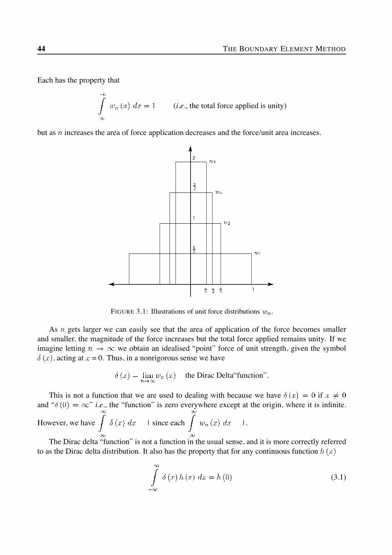
Each has the property that

(i.e., the total force applied is unity)

but as increases the area of force application decreases and the force/unit area increases.

FIGURE 3.1: Illustrations of unit force distributions .

As gets larger we can easily see that the area of application of the force becomes smallerand smaller, the magnitude of the force increases but the total force applied remains unity. If weimagine letting we obtain an idealised “point” force of unit strength, given the symbol

, acting at = 0. Thus, in a nonrigorous sense we have

the Dirac Delta“function”.

This is not a function that we are used to dealing with because we have ifand “ ” i.e., the “function” is zero everywhere except at the origin, where it is infinite.

However, we have since each .

The Dirac delta “function” is not a function in the usual sense, and it is more correctly referredto as the Dirac delta distribution. It also has the property that for any continuous function

(3.1)

3.2 THE DIRAC-DELTA FUNCTION AND FUNDAMENTAL SOLUTIONS 45

A rough proof of this is as follows

by definition of

by definition of

by the Mean Value Theorem, where

since and as

The above result (Equation (3.1)) is often used as the defining property of the Dirac delta inmore rigorous derivations. One does not usually talk about the values of the Dirac delta at aparticular point, but rather its integral behaviour. Some properties of the Dirac delta are listedbelow

(3.2)

(Note: is the Dirac delta distribution centred at instead of )

(3.3)

where =ifif

(i.e., the Dirac Delta function is the slope of the Heaviside2

step function.)

(3.4)

(i.e., the two dimensional Dirac delta is just a product of two one-dimensional Dirac deltas.)

3.2.2 Fundamental solutionsWe develop here the fundamental solution (also called the freespace Green’s3 function) for Laplace’sEquation in two variables. The fundamental solution of a particular equation is the weighting func-tion that is used in the boundary element formulation of that equation. It is therefore important tobe able to find the fundamental solution for a particular equation. Most of the common equations

2Oliver Heaviside (1850-1925) was a British physicist, who pioneered the mathematical study of electrical circuitsand helped develop vector analysis.

3George Green (1793-1841) was a self-educated miller’s son. Most widely known for his integral theorem (theGreen-Gauss theorem).


have well-known fundamental solutions (see Appendix 3.16). We briefly illustrate here how to finda simple fundamental solution.

Consider solving the Laplace Equation in some domain .The fundamental solution for this equation (analogous to a particular solution in ODE work) is

a solution of

(3.5)

in (i.e., we solve the above without reference to the original domain or original boundaryconditions). The method is to try and find solution to in which contains a singularityat the point . This is not as difficult as it sounds. We expect the solution to be symmetricabout the point since is symmetric about this point. So we adopt a localpolar coordinate system about the singular point .

Let

Then, from Section 1.8 we have

(3.6)

For and owing to symmetry, is zero. Thus Equation (3.6) becomes

This can be solved by straight (one-dimensional) integration. The solution is

(3.7)

Note that this function is singular at as required.To find and we make use of the integral property of the Delta function. From Equa-

tion (3.5) we must have

(3.8)

where is any domain containing .We choose a simple domain to allow us to evaluate the above integrals. If is a small disk of

3.2 THE DIRAC-DELTA FUNCTION AND FUNDAMENTAL SOLUTIONS 47

FIGURE 3.2: Domain used to evaluate fundamental solution coefficients.

radius centred at (Figure 3.2) then from the Green-Gauss theorem

is the surface of the disk

since is a disk centred at so and are in the same direction

from Equation (3.7), and the fact that is a disc of radius

Therefore, from Equation (3.8)

So we have

remains arbitrary but usually put equal to zero, so that the fundamental solution for the two-dimensional Laplace Equation is

(3.9)


where (singular at the point ).The fundamental solution for the three-dimensional Laplace Equation can be found by a similar

technique. The result is

where is now a distance measured in three-dimensions.

3.3 The Two-Dimensional Boundary Element MethodWe are now at a point where we can develop the boundary element method for the solution of

in a two-dimensional domain . The basic steps are in fact quite similar to those used forthe finite element method (refer Section 2.1). We firstly must form an integral equation from theLaplace Equation by using a weighted integral equation and then use the Green-Gauss theorem.From Section 2.4 we have seen that

(3.10)

This was the starting point for the finite element method. To derive the starting equation forthe boundary element method we use the Green-Gauss theorem again on the second integral. Thisgives

(3.11)

For the Galerkin FEM we chose , the weighting function, to be , one of the basis functionsused to approximate . For the boundary element method we choose to be the fundamentalsolution of Laplace’s Equation derived in the previous section i.e.,

where (singular at the point ).Then from Equation (3.11), using the property of the Dirac delta

(3.12)

i.e., the domain integral has been replaced by a point value.

3.3 THE TWO-DIMENSIONAL BOUNDARY ELEMENT METHOD 49

Thus Equation (3.11) becomes

(3.13)

This equation contains only boundary integrals (and no domain integrals as in Finite Elements)and is referred to as a boundary integral equation. It relates the value of at some point insidethe solution domain to integral expressions involving and over the boundary of the solutiondomain. Rather than having an expression relating the value of at some point inside the domainto boundary integrals, a more useful expression would be one relating the value of at some pointon the boundary to boundary integrals. We derive such an expression below.

The previous equation (Equation (3.13)) holds if (i.e., the singularity of Dirac Deltafunction is inside the domain). If is outside then

since the integrand of the second integral is zero at every point except and this point isoutside the region of integration. The case which needs special consideration is when the singularpoint is on the boundary of the domain . This case also happens to be the most importantfor numerical work as we shall see. The integral expression we will ultimately obtain is simplyEquation (3.13) with replaced by . We can see this in a non-rigorous way asfollows. When was inside the domain, we integrated around the entire singularity of theDirac Delta to get in Equation (3.13). When is on the boundary we only have half ofthe singularity contained inside the domain, so we integrate around one-half of the singularity toget . Rigorous details of where this coefficient comes from are given below.

Let denote the point . In order to be able to evaluate in this case we

enlarge to include a disk of radius about (Figure 3.3). We call this enlarged region andlet .

Now, since is inside the enlarged region , Equation (3.13) holds for this enlarged domaini.e.,

(3.14)

We must now investigate this equation as . There are integrals to consider, and we look ateach of these in turn.


FIGURE 3.3: Illustration of enlarged domain when singular point is on the boundary.

Firstly consider

by definition of

since on

since on

by the mean value theorem for a surface with a unique tangent at .Thus

(3.15)

By a similar process we obtain

(3.16)

since as .

3.3 THE TWO-DIMENSIONAL BOUNDARY ELEMENT METHOD 51

It only remains to consider the integrand over . For “nice” integrals (which includes theintegrals we are dealing with here) we have

(nice integrand) (nice integrand)

since as .Note: If the integrand is too badly behaved we cannot always replace by in the limit and

one must deal with Cauchy Principal Values. (refer Section 4.11)Thus we have

(3.17)

(3.18)

Combining Equations (3.14)–(3.18) we get

or

where (i.e., singular point is on the boundary of the region).Note: The above is true if the point is at a smooth point (i.e., a point with a unique tangent) on

the boundary of . If happens to lie at some nonsmooth point e.g. a corner, then the coefficientis replaced by where is the internal angle at (Figure 3.4).

FIGURE 3.4: Illustration of internal angle .


Thus we get the boundary integral equation.

(3.19)

where

ifif and smooth at

internal angle if and not smooth at

For three-dimensional problems, the boundary integral equation expression above is the same,with

ifif and smooth at

inner solid angleif and not smooth at

Equation (3.19) involves only the surface distributions of and and the value of at a

point . Once the surface distributions of and are known, the value of at any pointinside can be found since all surface integrals in Equation (3.19) are then known. The procedureis thus to use Equation (3.19) to find the surface distributions of and and then (if required)use Equation (3.19) to find the solution at any point . Thus we solve for the boundary datafirst, and find the volume data as a separate step.

Since Equation (3.19) only involves surface integrals, as opposed to volume integrals in a finiteelement formulation, the overall size of the problem has been reduced by one dimension (fromvolumes to surfaces). This can result in huge savings for problems with large volume to surfaceratios (i.e., problems with large domains). Also the effort required to produce a volume mesh of acomplex three-dimensional object is far greater than that required to produce a mesh of the surface.Thus the boundary element method offers some distinct advantages over the finite element methodin certain situations. It also has some disadvantages when compared to the finite element methodand these will be discussed in Section 3.6. We now turn our attention to solving the boundaryintegral equation given in Equation (3.19).

3.4 NUMERICAL SOLUTION PROCEDURES FOR THE BOUNDARY INTEGRAL EQUATION 53

3.4 Numerical Solution Procedures for the Boundary IntegralEquation

The first step is to discretise the surface into some set of elements (hence the name boundaryelements).

(3.20)

(b)(a)

FIGURE 3.5: Schematic illustration of a boundary element mesh (a) and a finite element mesh (b).

Then Equation (3.19) becomes

(3.21)

Over each element we introduce standard (finite element) basis functions

and (3.22)

where are values of and on element and are values of and at node onelement .

These basis functions for and can be any of the standard one-dimensional finite elementbasis functions (although we are dealing with a two-dimensional problem, we only have to inter-polate the functions over a one-dimensional element). In general the basis functions used for anddo not have to be the same (typically they are) and these basis functions can even be different to

the basis functions used for the geometry, but are generally taken to be the same (this is termed anisoparametric formulation).


This gives

(3.23)

This equation holds for any point on the surface . We now generate one equation per node byputting the point to be at each node in turn. If is at node , say, then we have

(3.24)

where is the fundamental solution with the singularity at node (recall is , whereis the distance from the singularity point). We can write Equation (3.24) in a more abbreviated

form as

(3.25)

where

and (3.26)

Equation (3.25) is for node and if we have nodes, then we can generate equations.We can assemble these equations into the matrix system

(3.27)

(compare to the global finite element equations ) where the vectors and are the vectorsof nodal values of and . Note that the th component of the matrix in general is not andsimilarly for .

At each node, we must specify either a value of or (or some combination of these) to have awell-defined problem. We therefore have equations (the number of nodes) and have unknownsto find. We need to rearrange the above system of equations to get

(3.28)

where is the vector of unknowns. This can be solved using standard linear equation solvers,although specialist solvers are required if the problem is large (refer [todo : Section ???]).

The matrices and (and hence ) are fully populated and not symmetric (compare to thefinite element formulation where the global stiffness matrix is sparse and symmetric). Thesize of the and matrices are dependent on the number of surface nodes, while the matrixis dependent on the number of finite element nodes (which include nodes in the domain). As

3.5 NUMERICAL EVALUATION OF COEFFICIENT INTEGRALS 55

mentioned earlier, it depends on the surface to volume ratio as to which method will generate thesmallest and quickest solution.

The use of the fundamental solution as a weight function ensures that the and matricesare generally well conditioned (see Section 3.5 for more on this). In fact the matrix is diagonallydominant (at least for Laplace’s equation). The matrix is therefore also well conditioned andEquation (3.28) can be solved reasonably easily.

The vector contains the unknown values of and on the boundary. Once this has beenfound, all boundary values of and are known. If a solution is then required at a point inside thedomain, then we can use Equation (3.25) with the singular point located at the required solutionpoint i.e.,

(3.29)

The right hand side of Equation (3.29) contains no unknowns and only involves evaluating thesurface integrals using the fundamental solution with the singular point located at .

3.5 Numerical Evaluation of Coefficient IntegralsWe consider in detail here how one evaluates the and integrals for two-dimensional problems.These integrals typically must be evaluated numerically, and require far more work and effort thanthe analogous finite element integrals.

Recall that

and

where

distance measured from node

In terms of a local coordinate we have

(3.30)

(3.31)


The Jacobian can be found by

(3.32)

where represents the arclength and and can be found by straight differentiation of the

interpolation expression for and .The fundamental solution is

where are the coordinates of node .

To find we note that

(3.33)

where is a unit outward normal vector. To find a unit normal vector, we simply rotate the tangentvector (given by ) by in the appropriate direction and then normalise.

Thus every expression in the integrands of the and integrals can be found at any value of, and the integrals can therefore be evaluated numerically using some suitable quadrature schemes.If node is well removed from element then standard Gaussian quadrature can be used to

evaluate these integrals. However, if node is in (or close to it) we see that approaches 0and the fundamental solution tends to . The integral still exists, but the integrand becomessingular. In such cases special care must be taken - either by using special quadrature schemes,large numbers of Gauss points or other special treatment.

The integrals for which node lies in element are in general the largest in magnitude andlead to the diagonally dominant matrix equation. It is therefore important to ensure that theseintegrals are calculated as accurately as possible since these terms will have most influence on thesolution. This is one of the disadvantages of the BEM - the fact that singular integrands must beaccurately integrated.

A relatively straightforward way to evaluate all the integrals is simply to use Gaussian quadra-ture with varying number of quadrature points, depending on how close or far the singular point isfrom the current element. This is not very elegant or efficient, but has the benefit that it is relativelyeasy to implement. For the case when node is contained in the current element one can use specialquadrature schemes which are designed to integrate log-type functions. These are to be preferredwhen one is dealing with Laplace’s equation. However, these special log-type schemes cannot beso readily used on other types of fundamental solution so for a general purpose implementation,Gaussian quadrature is still the norm. It is possible to incorporate adaptive integration schemesthat keep adding more quadrature points until some error estimate is small enough, or also to sub-divide the current element into two or more smaller elements and evaluate the integral over each

3.6 THE THREE-DIMENSIONAL BOUNDARY ELEMENT METHOD 57

(a)

node

node

(b)

FIGURE 3.6: Illustration of the decrease in as node approaches element .

subelement. It is also possible to evaluate the “worst” integrals by using simple solutions to thegoverning equation, and this technique is the norm for elasticity problems (Section 4.11). Detailson each of these methods is given in Section 3.8. It should be noted that research still continues inan attempt to find more efficient ways of evaluating the boundary element integrals.

3.6 The Three-Dimensional Boundary Element MethodThe three-dimensional boundary element method is very similar to the two-dimensional bound-ary element method discussed above. As noted above, the three-dimensional boundary integralequation is the same as the two-dimensional equation (3.19), with and being defined asin Section 3.3. The numerical solution procedure also parallels that given in Section 3.4, and theexpressions given for and apply equally well to the three-dimensional case. The only realdifference between the two procedures is how to numerically evaluate the terms in each integrandof these coefficient integrals.

As in Section 3.5 we illustrate how to evaluate each of the terms in the integrand of and .


The relevant expressions are

(3.34)

(3.35)

The fundamental solution is

where

where are the coordinates of node . As before we use to find .The unit outward normal is found by normalising the cross product of the two tangent vectors

and (it relies on the user of any BEM code to

ensure that the elements have been defined with a consistent set of element coordinates and ).The Jacobian is given by (where and are the two tangent vectors).

Note that this is different for the determinant in a two-dimensional finite element code - in thatcase we are dealing with a two-dimensional surface in two-dimensional space, whereas here wehave a (possibly curved) two-dimensional surface in three-dimensional space.

The integrals are evaluated numerically using some suitable quadrature schemes (see Sec-tion 3.8) (typically a Gauss-type scheme in both the and directions).

3.7 A Comparison of the FE and BE MethodsWe comment here on some of the major differences between the two methods. Depending on theapplication some of these differences can either be considered as advantageous or disadvantageousto a particular scheme.

1. FEM: An entire domain mesh is required.BEM: A mesh of the boundary only is required.Comment: Because of the reduction in size of the mesh, one often hears of people sayingthat the problem size has been reduced by one dimension. This is one of the major pluses of

3.7 A COMPARISON OF THE FE AND BE METHODS 59

the BEM - construction of meshes for complicated objects, particularly in 3D, is a very timeconsuming exercise.

2. FEM: Entire domain solution is calculated as part of the solution.BEM: Solution on the boundary is calculated first, and then the solution at domain points (ifrequired) are found as a separate step.Comment: There are many problems where the details of interest occur on the boundary, orare localised to a particular part of the domain, and hence an entire domain solution is notrequired.

3. FEM: Reactions on the boundary typically less accurate than the dependent variables.BEM: Both and of the same accuracy.

4. FEM: Differential Equation is being approximated.BEM: Only boundary conditions are being approximated.Comment: The use of the Green-Gauss theorem and a fundamental solution in the formu-lation means that the BEM involves no approximations of the differential Equation in thedomain - only in its approximations of the boundary conditions.

5. FEM: Sparse symmetric matrix generated.BEM: Fully populated nonsymmetric matrices generated.Comment: The matrices are generally of different sizes due to the differences in size ofthe domain mesh compared to the surface mesh. There are problems where either methodcan give rise to the smaller system and quickest solution - it depends partly on the volumeto surface ratio. For problems involving infinite or semi-infinite domains, BEM is to befavoured.

6. FEM: Element integrals easy to evaluate.BEM: Integrals are more difficult to evaluate, and some contain integrands that becomesingular.Comment: BEM integrals are far harder to evaluate. Also the integrals that are the mostdifficult (those containing singular integrands) have a significant effect on the accuracy ofthe solution, so these integrals need to be evaluated accurately.

7. FEM: Widely applicable. Handles nonlinear problems well.BEM: Cannot even handle all linear problems.Comment: A fundamental solutionmust be found (or at least an approximate one) before theBEM can be applied. There are many linear problems (e.g., virtually any nonhomogeneousequation) for which fundamental solutions are not known. There are certain areas in whichthe BEM is clearly superior, but it can be rather restrictive in its applicability.

8. FEM: Relatively easy to implement.BEM: Much more difficult to implement.Comment: The need to evaluate integrals involving singular integrands makes the BEM atleast an order of magnitude more difficult to implement than a corresponding finite elementprocedure.


3.8 More on Numerical IntegrationThe BEM involves integrals whose integrands in generally become singular when the source pointis contained in the element of integration. If one uses constant or linear interpolation for thegeometry and dependent variable, then it is possible to obtain analytic expressions to most (if notall) of the integrals that will appear in the BEM (at least for two-dimensional problems). Theexpressions can become quite lengthy to write down and evaluate, but benefit from the fact thatthey will be exact. However, when one begins to use general curved elements and/or solve three-dimensional problems then the integrals will not be available as analytic expressions. The basictool for evaluation of these integrals is quadrature. As discussed in Section 2.8 a one-dimensionalintegral is approximated by a sum in which the integrand is evaluated at certain discrete points orabscissa

where are the weights and are the abscissa.The weights and abscissa for the Gaussian quadrature scheme of order are chosen so that the

above expression will exactly integrate any polynomial of degree or less. For the numericalevaluation of two or three-dimensional integrals, a Gaussian scheme can be used of each variableof integration if the region of integration is rectangular. This is generally not the optimal choicefor the weights and abscissae but it allows easy extension to higher order integration.

3.8.1 Logarithmic quadrature and other special schemesLow order Gaussian schemes are generally sufficient for all FEM integrals, but that is not thecase for BEM. For a two-dimensional BEM solution of Laplace’s equation, integrals of the form

will be required. It is relatively common to use logarithmic schemes for this.

These are obtained by approximating the integral as

i.e., the log function has been factored out.In the same way as Gaussian quadrature schemes were developed in Section 2.8, log quadrature

schemes can be developed which will exactly integrate polynomial functions . Tables of theseare given below

It is possible to develop similar quadrature schemes for use in the BEM solution of other PDEs,which use different fundamental solutions to the log function. The problem with this approach isthe lack of generality - each new equation to be used requires its own special quadrature scheme.

3.9 THE BOUNDARY ELEMENT METHOD APPLIED TO OTHER ELLIPTIC PDES 61

Abscissas = Weight Factors =

2 0.112009 0.718539 3 0.063891 0.513405 4 0.041448 0.3834640.602277 0.281461 0.368997 0.391980 0.245275 0.386875

0.766880 0.094615 0.556165 0.1904350.848982 0.039225

TABLE 3.1: Abscissas and weight factors for Gaussian integration for integrands with alogarithmic singularity.

3.8.2 Special solutionsAnother approach, particularly useful if Cauchy principal values are to be found (see Section 4.11)is to use special solutions of the governing equation to find one or more of the more difficultintegrals.

For example is a solution to Laplaces’ equation (assuming the boundary conditionsare set correctly). Thus if one sets both and in Equation (3.27) at every node according tothe solution , one can then use this to solve for some entry in either the or matrix(typically the diagonal entry since this is the most important and difficult to find). Further solutionsto Laplaces equation (e.g., ) can be used to find the other matrix entries (or just usedto check the accuracy of the matrices).

3.9 The Boundary Element Method Applied to other EllipticPDEs

Helmholtz, modified Helmholtz (CMISS example) Poisson Equation (domain integral and MRM,DRM, Monte-carlo integration.

3.10 Solution of Matrix EquationsThe standard BEM approach results in a system of equations of the form (refer (3.28)).As mentioned above the matrix is generally well conditioned, fully populated and nonsymmet-ric. For small problems, direct solution methods, based on LU factorisations, can be used. As theproblem size increases, the time taken for the matrix solution begins to dominate the matrix assem-bly stage. This usually occurs when there is between and degrees of freedom, although itis very dependent on the implementation of the BE method. The current technique of favour in theBE community for solution of large BEMmatrix equations is a preconditioned Conjugate Gradientsolver. Preconditioners are generally problem dependent - what works well for one problem maynot be so good for another problem. The conjugate gradient technique is generally regarded as asolution technique for (sparse) symmetric matrix equations.


FIGURE 3.7: Coupled finite element/boundary element solution domain.

3.11 Coupling the FE and BE techniquesThere are undoubtably situations which favour FEM over BEM and vice versa. Often one problemcan give rise to a model favouring one method in one region and the other method in another regioneg. in a detailed analysis of stresses around a foundation one needs FEM close to the foundation tohandle nonlinearities, but to handle the semi-infinite domain (well removed from the foundation),BEM is better. There has been a lot of research on coupling FE and BE procedures - we willonly talk about the basic ideas and use Laplace’s Equation to illustrate this. There are at least twopossible methods.

1. Treat the BEM region as a finite element and combine with FEM

2. Treat the FEM region as an equivalent boundary element and combine with BEM

Note that these are essentially equivalent - the use of one or the other depends on the problem,in the sense of which part is more dominant FEM or BEM)

Consider the region shown in Figure 3.7, where

FEM regionBEM regionFEM boundaryBEM boundaryinterface boundary

The BEM matrices for can be written as

(3.36)

where is a vector of the nodal values of and is a vector of the nodal values ofThe FEM matrices for can be written as

(3.37)

3.11 COUPLING THE FE AND BE TECHNIQUES 63

where is the stiffness matrix and is the load vector.To apply method (i.e., treating BEM as an equivalent FEM region) we get (from Equa-

tion (3.36))

(3.38)

If we recall what the elements of in Equation (3.37) contained, then we can convert inEquation (3.38) to an equivalent load vector by weighting the nodal values of by the appropriatebasis functions, producing a matrix i.e.,

Therefore Equation (3.38) becomes

i.e.,

where

an equivalent stiffness matrix obtain from BEM.Therefore we can assemble this together with original FEM matrix to produce an FEM-type

system for the entire region .Notes:

1. is in general not symmetric and not sparse. This means that different matrix equationsolvers must be used for solving the new combined FEM-type system (most solvers in FEMcodes assume sparse and symmetric). Attempts have been made to “symmetricise” thematrix - of doubtful quality. (e.g., replace by - often yields inaccurateresults).

2. On nodal values of and are unknown. One must make use of the following

( is continuous)

( is continuous, but )

To apply method (i.e., to treat the FEM region as an equivalent BEM region) we firstly notethat, as before, . Applying this to (3.37) yields an equivalent BEM system.This can be assembled into the existing BEM system (using compatability conditions) and useexisting BEM matrix solvers.Notes:

1. This approach does not require any matrix inversion and is hence easier (cheaper) to imple-ment

2. Existing BEM solvers will not assume symmetric or sparse matrices therefore no new matrixsolvers to be implemented


3.12 Other BEM techniquesWhat we have mentioned to date is the so-called singular (direct) BEM. Given a BIE there areother ways of solving the Equation although these are not so widely used.

3.12.1 Trefftz methodTrefftz was the first person to perform a BEM calculation (in 1917 - calculated the value (numer-ical) of the contraction coefficient of a round jet issuing from an infinite tank - a nonlinear freesurface problem). This method basically uses a “complete” set of solutions instead of a Funda-mental Solution. e.g., Consider Laplaces Equation in a (bounded) domain

weighted residuals if

The procedure is to express as a series of (complete) functions satisfying Laplace’s equationwith coefficients which need to be numerically determined through utilisation of the boundaryconditions.Notes:

1. Doesn’t introduce singular functions so integrals are easy to evaluate

2. Must find a (complete) set of functions (If you just use usual approximations for matrixsystem is not diagonally dominant so not so good)

3. Method is not so popular - Green’s functions more widely available that complete systems

3.12.2 Regular BEMConsider the BIE for Laplace’s equation

with

The usual procedure is to put point at each solution variable node - creating an equation for eachnode. This leads to singular integrands.

Another possibility is to put point outside of the domain - this yields

3.13 SYMMETRY 65

Following discretisation as before gives

- an equation involving and at each surface node.By placing the point (the singular point) at other distinct points outside one can generate

as many equations as there are unknowns (or more if required).Notes:

1. This method does not involve singular integrands, so that integrals are inexpensive to calcu-late.

2. There is considerable choice for the location of the point . Often the set of Equationsgenerated are ill-conditioned unless chosen carefully. In practise is chosen along the unitoutward normal of the surface at each solution variable node. The distance along each nodeis often found by experimentation - various research papers suggesting “ideal” distances(Patterson & Shiekh).

3. This method is not very popular.

4. The idea of placing the singularity point away from the solution variable node is often ofuse in other situations e.g., Exterior Acoustic Problems. For an acoustic problem (governedby Helmholtz Equation ) in an unbounded region the system of Equations pro-duced by the usual (singular) BEM approach is singular for certain “fictitious” frequencies(i.e., certain values of ). To overcome this further equations are generated (by placing thesingular point at various locations outside ). The system of equations are then overde-termined and are solved in a least squares sense.

3.13 SymmetryConsider the problem given in Figure 3.8 (the domain is outside the circle). Both the boundaryconditions and the governing Equation exhibit symmetry about the vertical axis. i.e., putting to

makes no difference to the problem formulation. Thus the solution has the propertythat . This behaviour can be found in many problems and we can makeuse of this as follows. The Boundary Element Equation is (with (i.e., is even) constantelements)

(3.39)


FIGURE 3.8: A problem exhibiting symmetry.

We have Equations and unknowns (allowing for the boundary conditions). From symmetrywe know that (refer to Figure 3.9).

(3.40)

So we can write

(3.41)

for nodes . (The Equations for nodes are the same as the Equationsfor nodes ). The above Equations have only unknowns.

If we define

(3.42)

(3.43)

then we can write Equation (3.41) as

(3.44)

and solve as before. (This procedure has halved the number of unknowns.)

3.14 AXISYMMETRIC PROBLEMS 67

FIGURE 3.9: Illustration of a symmetric mesh.

Note: Since this means that the integrals over the elements to will nevercontain a singularity arising from the fundamental solution, except possibly on the axis of symme-try if linear or higher order elements are used.

An alternative approach to the method above arises from the implied no flux across the axis.This approach ignores the negative axis and considers the half plane problem shown.

However now the surface to be discretised extends to infinity in the positive and negativedirections and the resulting systems of equations produced is much larger.

Further examples of how symmetry can be used (e.g., radial symmetry) are given in the nextsection.

3.14 Axisymmetric ProblemsIf a three-dimensional problem exhibits radial or axial symmetry (i.e., ) itis possible to reduce the two-dimensional integrals appearing in the standard boundary Equationto one-dimensional line integrals and thus substantially reduce the amount of computer time thatwould otherwise be required to solve the fully three-dimensional problem. The first step in such aprocedure is to write the standard boundary integral equation in terms of cylindrical polarsi.e.,

(3.45)

where and are the polar coordinates of and respectively, and is theintersection of and semi-plane (Refer Figure 3.10). (n.b. is a point on the surface beingintegrated over.)


FIGURE 3.10: Illustration of surface for an axisymmetric problem.

FIGURE 3.11: The distance from the source point ( ) to the point of interest ( ) in terms ofcylindrical polar coordinates.

For three-dimensional problems governed by Laplace’s equation

where is the distance from to . From Figure 3.11

(3.46)

3.15 INFINITE REGIONS 69

We define

where (3.47)

and is the complete elliptic integral of the first kind.is called the axisymmetric fundamental solution and is the Green’s function for a ring source

as opposed to a point source. i.e., is a solution of

(3.48)

instead of

(3.49)

where is the dirac delta centered at the point and is the dirac delta centered on thering .

Unlike the two- and three-dimensional cases, the axisymmetric fundamental solution cannot bewritten as simply a function of the distance between two points and , but it also depends uponthe distance of these points to the axis of revolution.

We also define

(3.50)

For Laplace’s equation Equation (3.50) becomes

(3.51)

where is the complete elliptic integral of the second kind.Using Equation (3.47) and Equation (3.50) we can write Equation (3.45) as

(3.52)

and the solution procedure for this Equation follows the same lines as the solution procedure givenpreviously for the two-dimensional version of boundary element method.

3.15 Infinite RegionsThe boundary integral equations we have been using have been derived assuming the domainis bounded (although this was never stated). However all concepts presented thus far are also


FIGURE 3.12: Derivation of infinite domain boundary integral equations.

valid for infinite regular (i.e., nice) regions provided the solution and its normal derivative behaveappropriately as .

Consider the problem of solving outside some surface .is the centre of a circle (or sphere in three dimensions) of radius centred at some point on

and surrounding (see Figure 3.12). The boundary integral equations for the bounded domaincan be written as

(3.53)

If we let the radius Equation (3.53) will only be valid for the points on if

(3.54)

If this is satisfied, the boundary integral Equation for will be as expected i.e.,

(3.55)

3.15 INFINITE REGIONS 71

For three-dimensional problems with

where

where is the Jacobian and represents the asymptotic behaviour of the function as. In this case Equation (3.53) will be satisfied if behaves at most as so that

. These are the regularity conditions at infinity and these ensure that each term in theintegral Equation (3.53) behaves at most as (i.e., each term will as )

For two-dimensional problems with we require to behave as so that. For almost all well posed infinite domain problems the solution behaves appropri-

ately at infinity.


3.16 Appendix: Common Fundamental Solutions

3.16.1 Two-Dimensional equationsHere .

Laplace Equation

Solution

Helmholtz Equation

Solutionwhere is the Hankel funtion.

Wave Equation

where is the wave speed.

Solution

Diffusion Equation

where is the diffusivity.

Solution

Navier’s Equation for a point load in direction .

Solution

for a traction in direction where is Poisson’s ratio.

3.16.2 Three-Dimensional equationsHere .


Laplace Equation

Solution

Helmholtz Equation

Solution

Wave Equation

where is the wave speed.

Solution

Navier’s Equation for a isotropic homogenenous Kelvin

solution for a point load in direction .Solution

for a displacement in direction where is Poisson’sratio and is the shear modulus.

3.16.3 Axisymmetric problemsLaplace For see Equation (3.47) and for see Equation (3.51)

3.17 CMISS Examples1. 2D steady-state heat conduction inside an annulus To determine the steady-state heat con-duction inside an annulus run the CMISS example .

2. 3D steady-state heat conduction inside a sphere. To determine the steady-state heat conduc-tion inside a sphere run the CMISS example .

3. CMISS comparison of 2-D FEM and BEM calculations To determine the CMISS comparisonof 2-D FEM and BEM calculations run examples and .

4. CMISS biopotential problems C4 and C5.

Chapter 4

Linear Elasticity

4.1 IntroductionTo analyse the stress in various elastic bodies we calculate the strain energy of the body in terms ofnodal displacements and then minimize the strain energy with respect to these parameters - a tech-nique known as the Rayleigh-Ritz. In fact, as we will show later, this leads to the same algebraicequations as would be obtained by the Galerkin method (now equivalent to virtual work) but thephysical assumptions made (in neglecting certain strain energy terms) are exposed more clearly inthe Rayleigh-Ritz method. We will first consider one-dimensional truss and beam elements, thentwo-dimensional plane stress and plane strain elements, and finally three-dimensional elasticity.

In all cases the steps are:

1. Evaluate the components of strain in terms of nodal displacements,

2. Evaluate the components of stress from strain using the elastic material constants,

3. Evaluate the strain energy for each element by integrating the products of stress and straincomponents over the element volume,

4. Evaluate the potential energy from the sum of total strain energy for all elements togetherwith the work done by applied boundary forces,

5. Apply the boundary conditions, e.g., by fixing nodal displacements,

6. Minimize the potential energy with respect to the unconstrained nodal displacements,

7. Solve the resulting system of equations for the unconstrained nodal displacements,

8. Evaluate the stresses and strains using the nodal displacements and element basis functions,

9. Evaluate the boundary reaction forces (or moments) at the nodes where displacement isconstrained.

76 LINEAR ELASTICITY

4.2 Truss ElementsConsider the one-dimensional truss of undeformed length in Figure 3.1 with end pointsand and making an angle with the x-axis. Under the action of forces in the - and -directions the right hand end of the truss displaces by in the -direction and in the -direction,relative to the left hand end.

FIGURE 4.1: A truss of initial length is stretched to a new length . Displacements of the righthand end relative to the left hand end are and in the - and - directions, respectively.

The new length is with axial strain

using and . Neglecting second order terms in the binomial expansion

, the strain for small displacements and is

(4.1)

The strain energy associated with this uniaxial stretch is

SE (4.2)

4.2 TRUSS ELEMENTS 77

where is the stress in the truss (of cross-sectional area ), linearly related to the strainvia Young’s modulus . We now substitute for from Equation (4.1) into Equation (4.2) and put

and , where and are the nodal displacements of the twoends of the truss

SE (4.3)

The potential energy is the combined strain energy from all trusses in the structure minus thework done on the structure by external forces. The Rayleigh-Ritz approach is to minimize thispotential energy with respect to the nodal displacements once all displacement boundary conditionshave been applied.

For example, consider the system of three trusses shown in Figure 4.2. A force ofis applied in the -direction at node . Node is a sliding joint and has zero displacement in they-direction only. Node is a pivot and therefore has zero displacement in both - and - directions.The problem is to find all nodal displacements and the stress in the three trusses.

node

node node

FIGURE 4.2: A system of three trusses.

The strain in truss (joining nodes and ) is




Since a force of acts at node in the -direction, the potential energy is

PEtrusses

Minimizing the potential energy with respect to the three unknowns , and gives

PE(4.4)

PE (4.5)

PE(4.6)

If we choose , and (e.g., timbertruss) then .

Equation (4.6) gives

Equation (4.4) gives

Equation (4.5) gives for two dimensions

Solving these last two equations gives and . Thus the strain in truss

is , in truss is and in truss is zero.The tension in truss is (tensile),

in truss is (compressive) and in truss is zero. The nodal reaction forces are shown inFigure 4.3.

4.3 BEAM ELEMENTS 79

FIGURE 4.3: Reaction forces for the truss system of Figure 4.2.

4.3 Beam ElementsSimple beam theory ignores all but axial strain and stress ( Young’s modulus)along the beam (assumed here to be in the x-direction). The axial strain is given by ,where is the lateral distance from the neutral axis in the plane of the bending and is the radius

of curvature in that plane. The bending moment is given by , where is the beam

crossectional area. Thus

(4.7)

(4.8)

where is the second moment of area of the beam cross-section. Thus, and

Equation (4.7) becomes

(4.9)

The slope of the beam is and the rate of change of slope is the curvature

(4.10)


Thus the bending moment is

(4.11)

and a force balance gives the shear force

(4.12)

and the normal force (per unit length of beam)

(4.13)

This last equation is the equilibrium equation for the beam, balancing the loading forces with theaxial stresses associated with beam flexure

(4.14)

The elastic strain energy stored in a bent beam is the sum of flexural strain energy and shearstrain energy, but this latter is ignored in the simple beam theory considered here. Thus, the(flexural) strain energy is

SE

where is taken along the beam and is the cross-sectional area of the beam.The external work associated with forces acting normal to the beam and moving through a

transverse displacement is . The potential energy is therefore

PE (4.15)

The finite element approximation for the transverse displacement must be able to representthe second derivative . A linear basis function has a zero second derivative and therefore cannotrepresent the flexural strain. The natural choice of basis function for beam deflection is in fact cubicHermite because the inter-element slope continuity of this basis ensures transmission of bendingmoment as well as shear force across element boundaries.

The boundary conditions associated with the th order equilibrium Equation (4.14) or the equa-

4.4 PLANE STRESS ELEMENTS 81

tions arising from minimum potential energy Equation (4.15) (which contain the square of nd

derivative terms) are more complex than the simple temperature or flux boundary conditions forthe (second order) heat equation. Three possible combinations of boundary condition with theirassociated reactions are

Boundary conditions Reactions

(i) Simply supported zero displacement shear forcezero moment slope

(ii) Cantilever zero displacement shear forcezero slope moment

(iii) Free end zero shear force displacementzero moment slope

4.4 Plane Stress ElementsFor two-dimensional problems, we define the displacement vector , strain vector

and stress vector . The stress-strain relation for two-dimensional plane stress:

(4.16)

can be written in matrix form

where . The strain components are given in terms of displacement

gradients by

(4.17)


The strain energy is

SE

The potential energy is

PE SE external work (4.18)

where represents the external forces acting on the elastic body.Following the steps outlined in Section 4.1 we approximate the displacement field with a

finite element basis , and calculate the strains

(4.19)

or

(4.20)

From Equation (4.18) the potential energy is therefore

PE

4.5 NAVIER’S EQUATION 83

where is the element stiffness matrix.

We next minimize the potential energy with respect to the nodal parameters and giving

(4.21)

4.5 Navier’s EquationThe Galerkin finite element equations for linear elasto-statics can be derived from a physicallyappealing argument, the principle of virtual work. Let be the stress vector acting over the surfaceenclosing a volume of material of mass density and let be the equailibrium external force

vector per unit area of surface (i.e., ). The equilibrium equation in is ( arethe components of stress) and by Cauchy’s formula, , where is a component of theunit normal to .

Now, the principle of virtual work equates the work done by the surface forces , inmoving through a virtual displacement to the work done by the stress vectorin moving through a compatible set of virtual diaplcements . Thus,

The Green-Gauss theorem, Equation (2.15):

(4.22)

is now used to replace the right hand surface integral by a volume integral; giving

Substituting the equilibrium relation into the right hand integral yields the virtualwork equation

(4.23)

where the internal work done due to the stress field is equated to the work due to internal bodyforces and external surface forces. Let and interpolate the virtual displacements


from their nodal values. i.e.,

so (4.24)

where and is the global node number of local node on elementThis gives

Since virtual dispalcements are arbitrary we get

We now have

(4.25)

We wish to find , the coefficient of (i.e., the displacement at node in direction )For linear, isotropic, homogeneous materials we have the generalised Hookes Law.

(4.26)

where and are Lames constants. Also we put this gives

(4.27)

Note that a coefficient of also comes from (the first term)

4.6 NOTE ON CALCULATING NODAL LOADS 85

So

So the coefficient of can be calculated by

Note: there is no sum for .The expression for can be simplified to give

(4.28)

where , i.e., the metric tensor resulting from the inner product of basis vectors.

4.6 Note on Calculating Nodal LoadsIf a normal boundary stress is known it is necessary to compute the equivalent nodal load forces torepresent the distributed load. For example, consider a uniform load applied to the edgeof the plane stress element in Figure 4.4a.

The nodal load vector in Equation (4.21) has components

(4.29)

where is the normalized element coordinate along the side of length loaded by the constantstress . If the element side has a linear basis, Equation (4.29) gives


as shown in Figure 4.4b. If the element side has a quadratic basis, Equation (4.29) gives

as shown in Figure 4.4c. A node common to two elements will receive contributions from bothelements, as shown in Figure 4.4d.

(a) (b) (c) (d)

FIGURE 4.4: A uniform boundary stress applied to the element side in (a) is equivalent to nodalloads of and for the linear basis used in (b) and to , and for the quadraticbasis used in (c). Two adjacent quadratic elements both contribute to a common node in (d), where

the element length is now .

4.7 Three-Dimensional ElasticityRecall that if a body is in equilibrium then we have

(4.30)

where are the components of the stress tensor ( is the component of the traction or stressvector in the th direction which is acting on the face of a rectangle whose normal is in the th

direction), and is the body force/unit volume (e.g., )Recall also that the components of the (small) strain tensor are

(4.31)

4.7 THREE-DIMENSIONAL ELASTICITY 87

where is the displacement vector (i.e., is the difference between the final and initial positionsof a material point in question).

(Note: We are assuming here that the displacement gradients are small compared to unity whichis the usual situation in solid mechanics. If we start dealing with materials such as rubber or livingtissue then we need to use the exact finite strain tensor).

The object of solving an elasticity problem is to find the distributions of stress and displacementin an elastic body, subject to a known set of body forces and prescribed stresses or displacementsat the boundaries. In the general three-dimensional case, this means finding stress components

and 3 displacements each as a function of position in the body. Currently we haveunknowns ( stresses, strains and displacements) and only equations.

An equation of state (stress-strain relation or constitutive law) is required. For a linear elasticmaterial we usually propose that depend linearly on . i.e.,

where are the components of a th order tensor.Symmetry reduces the number of unknowns to . If the material is isotropic (i.e., the material

response is independent of orientation of the material element) then we have the generalized Hook’sLaw.

(4.32)

or inversely

where , are Lames constants.Note: , are related to Young’s modules and Poisson’s ratio by

As long as the displacements are continuous functions of position then Equation (4.30), Equa-tion (4.31) and Equation (4.32) are sufficient to determine the unknown quantities. This canoften work with some smaller grouping of Equation (4.30), Equation (4.31) and Equation (4.32)e.g., If all boundary conditions are expressed in terms of displacements Equation (4.31) into Equa-tion (4.32) then into Equation (4.30) yields Navier’s equation.

These are the equations for displacements, Equation (4.31) yields strains and Equation (4.32)yields stresses.


4.8 Integral EquationUsing weighted residuals as before we can write

(4.33)

where is a (vector) weighting field. The are usually interpreted as a consistent set ofvirtual displacements (hence we use the notation instead of ).

Now

Therefore, by the divergence theorem

(4.34)

Thus combining Equation (4.33) and Equation (4.34) we have

(4.35)

where are the (surface) tractions (i.e., ).This statement Equation (4.35) is more usually derived from considering virtual work (we use

weighted residuals to tie in to Chapter 3). The principle of virtual work equates the internal workdue to the stress field (left hand side integral) to the work due to internal body forces and externalsurface forces. This statement is independent of the constitutive law of the material.

4.9 Linear Elasticity with Boundary ElementsEquation (4.35) is the starting point for the general finite element formulation (Section 4.7). Inthe above derivation, we have essentially used the Green-Gauss theorem once to move from Equa-tion (4.33) to Equation (4.35) (as was done for the derivation of the FEM equation for Laplace’s

4.9 LINEAR ELASTICITY WITH BOUNDARY ELEMENTS 89

equation). To continue, we firstly note that

where are the virtual strains corresponding to the virtual displacements.Using the constitutive law for linearly elastic materials (Equation (4.32)) we have

due to symmetry.Thus from the virtual work statement, Equation (4.35) and the above symmetry we have

(4.36)

This is known as Betti’s second reciprical work theorem or the Maxwell-Betti reciprocity relation-ship between two different elastic problems (the starred and unstarred variables) established on thesame domain.

Note that (i.e., ). Therefore Equation (4.36) can be written as

(4.37)

( represents the equilibrium state corresponding to the virtual displacements ).Note: What we have essentially done is use integration of parts to get Equation (4.35), then use

it again to get Equation (4.36) above (after noting the reciprocity between and ).Since the body forces, , are known functions, the second domain integral on the left hand

side of Equation (4.37) does not introduce any unknowns into the problem (more about this later).


The first domain integral contains unknown displacements in and it is this integral we wish toremove.

We choose the virtual displacements such that

(4.38)

(or equivalently ), where is the th component of a unit vector in the th directionand . We can interpret this as the body force components which correspond to apositive unit point load applied at a point in each of the three orthogonal directions.

Therefore

i.e., the volume integral is replaced with a point value (as for Laplace’s equation).Therefore, Equation (4.37) becomes

(4.39)

If each point load is taken to be independent then and can be written as

(4.40)(4.41)

where and represent the displacements and tractions in the th direction atcorresponding to a unit point force acting in the th direction ( ) applied at . Substituting theseinto Equation (4.39) (and equating components in each direction) yields

(4.42)

where (see later for ).This is known as Somigliana’s 1 identity for displacement.1Somigliana was an Italian Mathematician who published this result around 1894-1902.

4.10 FUNDAMENTAL SOLUTIONS 91

4.10 Fundamental SolutionsRecall from Equation (4.38) that satisfied

(4.43)

or equivalently

Navier’s equation for the displacements is

where = shear Modulus.Thus satisfy

(4.44)

The solutions to the above equation in either two or three dimensions are known as Kelvin 2’sfundamental solutions and are given by

(4.45)

for three-dimensions and for two-dimensional plane strain problems,

(4.46)

and

(4.47)

where for two-dimensional plane strain and three-dimensional problems respec-tively.

Here , the distance between load point ( ) and field point ( ),

and .

In addition the strains at an point due to a unit point load applied at in the th direction aregiven by

2Lord Kelvin (1824-1907) Scottish physicist who made great contributions to the science of thermodynamics


and the stresses are given by

where and are defined above.The plane strain expressions are valid for plane stress if is replaced by (This is a

mathematical equivalence of plane stress and plane strain - there are obviously physical differences.What the mathematical equivalence allows us to do is to use one program to solve both types ofproblems - all we have to do is modify the values of the elastic constants).

Note that in three dimensions

and for two dimensions

Somigliana’s identity (Equation (4.42)) is a continuous representation of displacements at anypoint . Consequently, one can find the stress at any firstly by combining derivativesof (4.42) to produce the strains and then substituting into Hooke’s law. Details can be found inBrebbia, Telles & Wrobel (1984b) pp 190–191, 255–258.

This yields

Note: One can find internal stress via numerical differentiation as in FE/FD but these are notas accurate as the above expressions.

Expressions for the new tensors and are on page 191 in (Brebbia et al. 1984b).

4.11 Boundary Integral EquationJust as we did for Laplace’s equation we need to consider the limiting case of Equation (4.42) asis moved to . (i.e., we need to find the equivalent of (in section 3) - called here .)

We use the same procedure as for Laplace’s equation but here things are not so easy.If we enlarge to as shown.

4.11 BOUNDARY INTEGRAL EQUATION 93

FIGURE 4.5: Illustration of enlarged domain when singular point is on the boundary.

Then Equation (4.42) can be written as

(4.48)

We need to look at each integral in turn as (i.e., from above). The only integral thatpresents a problem is the second integral. This can be written as

(4.49)

The first integral on the right hand side can be written as

by continuity of

(4.50)


Let

(4.51)

As , and we write the second integral of Equation (4.49) as

where we interpret this in the Cauchy Principal Value3sense.Thus as we get the boundary integral equation

(4.52)

(or, in brief (no body force), ) where the integral on the left hand

side is interpreted in the Cauchy Principal sense. In practical applications and the principal valueintegral can be found indirectly from using Equation (4.52) to represent rigid-body movements.

The numerical implementation of Equation (4.52) is similar to the numerical implementationof an elliptic equation (e.g., Laplace’s Equation). However, whereas with Laplace’s equation theunknowns were and (scalar quantities) here the unknowns are vector quantities. Thus it is

3What is a Cauchy Principle Value?Consider onThen

This is the Cauchy Principle Value of

But if we replace by then

(by definition of improper integration)

which does NOT exist. i.e., the integral does not exist in the proper sense, but it does in the Cauchy Principal Valuesense. However, if an integral exists in the proper sense, then it exists in the Cauchy Principal Value sense and the twovalues are the same.

4.12 BODY FORCES (AND DOMAIN INTEGRALS IN GENERAL) 95

more convenient to work with matrices instead of indicial notation.i.e., use

Then (in absence of a body force) we can write Equation (4.52) as

(4.53)

We can discretise the boundary as before and put , the singular point, at each node (eachnode has unknowns - displacements and tractions - we get equations per node). The overallmatrix equation

(4.54)

where ...and ...

where is the number nodes.

The diagonal elements of the matrix in Equation (4.54) (for three-dimensions, a x matrix)contains principal value components. If we have a rigid-body displacement of a finite body in anyone direction then we get

( = vector defining a rigid body displacement in direction )

(no sum on )

i.e., the diagonal entries of (the ’s) do not need to be determined explicitly. There is a similarresult for an infinite body.

4.12 Body Forces (and Domain Integrals in General)The body force gives rise to a domain integral although it does not give rise to any further unknownsin the system of equations. (This is because the body force is known - the fundamental solution


was chosen so that it removed all unknowns appearing in domain integrals).Thus Equation (4.52) is still classed as a Boundary Integral Equation. Integrals over the domain

containing known functions (eg body force integral) appear in many situations e.g., the Poissonequation yields a domain integral involving .

The question is how do we evaluate domain integrals such as those appearing in the boundaryintegral forumalation of such equations? Since the functions are known a coarse domain meshmay work.(n.b. Since the integral also contains the fundamental solution and may not be a“nice” region it is unlikely that it can be evaluated analytically). However, a domain mesh nullifiesone of the advantages of BEM - that of having to prepare only a boundary mesh.

In some cases domain integrals must be used but there are techniques developing to avoid manyof them. In some standard situations a domain integral can be transformed to a boundary integral.e.g., a body force arising from a constant gravitational load, or a centrifugal load due to rotationabout a fixed axis or the effect of a steady state thermal load can all be transformed to a boundaryintegral.

Firstly, let (the Galerkin tension) be related to by

(3D)

(2D)

Then

Under a constant gravitational load

which is a boundary integral.Unless the domain integrand is “nice” the above simple application of Green’s theorem won’t

work in general. There has been a considerable amount of research on domain integrals in BEMwhich has produced techniques for overcoming some domain methods. The two integrals of noteare the DRM, dual reciprocity method, developed around 1982 and the MRM, multiple reciprocitymethod, developed around 1988.


4.13 CMISS Examples1. To solve a truss system run CMISS example This solves the simple three truss systemshown in Figure 4.2.

2. To solve stresses in a bicycle frame modelled with truss elements run CMISS example .

Chapter 5

Transient Heat Conduction

5.1 IntroductionIn the previous discussion of steady state boundary value problems the principal advantage of thefinite element method over the finite difference method has been the greater ease with which com-plex boundary shapes can be modelled. In time-dependent problems the solution proceeds froman initial solution at and it is almost always convenient to calculate each new solution at aconstant time ( ) throughout the entire spatial domain . There is, therefore, no need to usethe greater flexibility (and cost) of finite elements to subdivide the time domain: finite differenceapproximations of the time derivatives are usually preferred. Finite difference techniques are intro-duced in Section 5.2 to solve the transient one dimensional heat equation. A combination of finiteelements for the spatial domain and finite differences for the time domain is used in Section 5.3 tosolve the transient advection-diffusion equation - a slight generalization of the heat equation.

5.2 Finite Differences

5.2.1 Explicit Transient Finite DifferencesConsider the transient one-dimensional heat equation

(5.1)

where is the conductivity and is the temperature, subject to the boundary conditionsand and the initial conditions . A finite difference approxi-

mation of this equation is obtained by defining a grid with spacing in the x-domain and inthe time domain, as shown in Figure 5.1.

Grid points are labelled by the indices (for the -direction) and(for the -direction). The temperature at the grid point is therefore labelled as

(5.2)

Finite difference equations are derived by writing Taylor Series expansions for

100 TRANSIENT HEAT CONDUCTION

about the grid point

(5.3)

(5.4)

(5.5)

where and represent all the remaining terms in the Taylor Series expansions.Adding Equations (5.3) and (5.4) gives

or

(5.6)

which is a “central difference” approximation of the second order spatial derivative.Rearranging Equation (5.5) gives a “difference” approximation of the first order time derivative

(5.7)

Substituting Equation (5.6) and Equation (5.7) into the transient heat equation Equation (5.1)gives the finite difference approximation

which is rearranged to give an expression for in terms of the values of at the th time step

(5.8)

Given the initial values of at (i.e., ), the values of for the next time stepare found from Equation (5.8) with . Applying Equation (5.8) iteratively for timesteps etc. yields the time dependent temperatures at the grid points (see Figure 5.1).This is an explicit finite difference formula because the value of depends only on the values of

at the previous time step and not on the neighbouring terms and atthe latest time step. The accuracy of the solution depends on the chosen values of and andin fact the stability of the scheme depends on these satisfying the Courant condition:

(5.9)

5.2 FINITE DIFFERENCES 101

x

xx x

... ...

:

FIGURE 5.1: A finite difference grid for the solution of the transient 1D heat equation. Theequation is centred at grid point shown by the . The lightly shaded region shows where thesolution is known at time step . With central differences in and a forward difference in anexplicit finite difference formula gives the solution at time step explicitly in terms of the

solution at the three points below it at step , as indicated by the dark shading.

5.2.2 Von Neumann Stability AnalysisThe concept behind the Von Neumann analysis is that all Fourier components decay as time isadvances or as they are processed by an iterative solver. Considering Equation (5.8), we canrearrange this to be of the form,

(5.10)

where . By subsituting the general Fourier component , we obtain,

(5.11)

If divide Equation (5.11) by, we obtain,

(5.12)

Equation (5.12) predicts the growth of any component (specified by or ) admitted by the


system. If all components are to decay,

for stability (5.13)

As the term in Equation (5.12) is always between and , we effective have the stablitycriteria that,

(5.14)

This condition will always hold if,

(5.15)

This can be rearranged to be of the form,

(5.16)

i.e., the time step should be at least half the size of the term

5.2.3 Higher Order ApproximationsAn improvement in accuracy and stability can be obtained by using a higher order approximationfor the time derivative. For example, if a central difference approximation is used for bycentering the equation at rather than we get

(5.17)

in place of Equation (5.7) and Equation (5.1) is approximated with the “Crank-Nicolson”formula

(5.18)

in which the spatial second derivative term is weighted by at the old time step and by at thenew time step . Notice that the finite difference time derivative has not changed - only thetime position at which it is centred. The price paid for the better accuracy (for a given ) andunconditional stability (i.e., stable for any ) is that Equation (5.18) is an implicit scheme - theequations for the new time step are now coupled in that depends on the neighbouring terms

and . Thus each new time step requires the solution of a system of coupled equations.

5.3 THE TRANSIENT ADVECTION-DIFFUSION EQUATION 103

xx

xx x

x

...

:

...

FIGURE 5.2: An implicit finite difference scheme based on central differences in , as well as ,which tie together the 6 points shown by . The equation is centred at the point ( ) shownby the . The lightly shaded region shows where the solution is known at time step . The dark

shading shows the region of the coupled equations.

A generalization of (5.18) is

(5.19)

in which the spatial second derivative of Equation (5.1) has been weighted by at the new time stepand by at the old time step. The original explicit forward difference scheme Equation (5.8)is recovered when and the implicit central difference (Crank-Nicolson) scheme (5.19) when

. An implicit backward difference scheme is obtained when .In the following section the transient heat equation is approximated for numerical analysis

by using finite differences in time and finite elements in space. We also generalize the partialdifferential equation to include an advection term and a source term.

5.3 The Transient Advection-Diffusion EquationConsider a linear parabolic equation

(5.20)

where is a scalar variable (e.g., the advection-diffusion equation, where is concentration ortemperature; then represents advective transport by a velocity field is the diffusivityand is source term. The ratio of advective to diffusive transport is characterised by the Pecletnumber where and is a characteristic length).


Applying the Galerkin weighted residual method to Equation (5.20) with weight gives

or

(5.21)

where is the normal derivative to the boundary .Putting and and summing the element contributions to the global equations,

Equation (5.21) can be represented by a system of first order ordinary differential equations,

(5.22)

where is the global mass matrix, the global stiffness matrix and a vector of global nodalunknowns with steady state values ( ) . The element contributions to and aregiven by

(5.23)

and

(5.24)

If the time domain is now discretized Equation (5.24) can be re-placed by

(5.25)

where is a weighting factor discussed in Section 5.2. Note that for the method is knownas the Crank-Nicolson-Galerkinmethod and errors arising from the time domain discretization are

. Rearranging Equation (5.25) as

(5.26)

gives a set of linear algebraic equations to solve at the new time step from the knownsolution at the previous time step .

The stability of the above scheme can be examined by expanding (assumed to be smoothly

5.3 THE TRANSIENT ADVECTION-DIFFUSION EQUATION 105

continuous in time) in terms of the eigenvectors (with associated eigenvalues ) of the matrix. Writing the initial conditions and steady state solution

, the set of ordinary differential equations Equation (5.22) has solution

(5.27)

The time-difference scheme Equation (5.26) on the other hand, with now replaced by a setof discrete values at each time step , can be written as the recursion formula

(5.28)

with solution

(5.29)

(You can verify that Equation (5.27) and Equation (5.29) are indeed the solutions of Equation (5.22)and Equation (5.25), respectively, by substituting and using .)

Comparing Equation (5.27) and Equation (5.29) shows that replacing the ordinary differentialequations (5.22) by the finite difference approximation Equation (5.25) is equivalent to replacingthe exponential in Equation (5.27) by the approximation

(5.30)

or, with ,

(5.31)

The stability of the numerical time integration scheme can now be investigated by examiningthe behaviour of this approximation to the exponential. For stability we require

(5.32)

since this term appears in Equation (5.29) raised to the power . The right hand inequality inEquation (5.32) is trivially satisfied, since and are all positive, and the left hand inequalitygives

or (5.33)

A consequence of Equation (5.33) is that the scheme is unconditionally stable if .


For the stability criterion is

(5.34)

If the exponential approximation given by Equation (5.31) is negative for any the solutionwill contain components which change sign with each time step . This oscillatory noise can beavoided by choosing

max(5.35)

where max is the largest eigenvalue in the matrix , but in practice this imposes a limit whichis too severe for and a small amount of oscillatory noise, associated with the high frequencyvibration modes of the system, is tolerated. Alternatively the oscillatory noise can be filtered outby averaging.

These theoretical results are explored numerically with a Crank-Nicolson-Galerkin scheme( ) in Figure 5.3, where the one-dimensional diffusion equation

on

subject to initial conditionsand boundary conditions

(5.36)

is solved for various time increments ( ) and element lengths ( ) for both linear and cubicHermite elements.

Decreasing from to with linear elements produces more oscillation because thesystem has moredegrees of freedom and leads to greater oscillation. At a sufficiently small theoscillations are negligible (bottom right, Figure 5.3). With this value of ( ) the numericalresults agree well with the exact solution (top, Figure 5.3) given by

(5.37)

5.4 Mass lumpingA technique known as mass lumping is sometimes used in which the mass matrix is replacedby a diagonal matrix having diagonal terms equal to the row sums. For example, consider the mass

5.4 MASS LUMPING 107

linear elements

x

x

x

x

x

(d)

x

xx

xlinear elements

xx

x

xx

xx

xx

xx

x

x x x

cubic elements

(c)

x x

Linear CNG withx x

(e)

xx

x

Exact solution

x

xxxxx

x

x

x x

x

x

(b)

linear elements

xx

xxx x xx

x

x

x

x

x

x x

x

x

FIGURE 5.3: Analytical and numerical solutions of the transient 1D heat equation showing theeffects of element size and time step size . The top graph shows the exact and approximatesolutions as functions of at various times. The lower graphs show the solution through time at the

specified positions and with various choices of and as indicated.


matrix ((5.23)) for a bilinear element (see Figure 1.9 and (1.6)).

and similarly and .

and similarly and .

and similarly .

therefore mass lumping

The element mass is effectively lumped at the element vertices. Such a scheme has computa-tional advantages when in Equation (5.26) because each component of the vector isobtained directly without the need to solve a set of coupled equations. This explicit time integrationscheme, however, is only conditionally stable (see (5.34)) and suffers from phase lag errors - seebelow. For evenly spaced elements the finite element scheme with mass lumping is equivalent tofinite differences with central spatial differences.

In Figure 5.4, the finite element and finite differences (lumped f.e. mass matrix) solutions ofthe one-dimensional advection-diffusion equation (5.20) with , ,are compared for the propogation and dispersion of an initial unit mass pulse at . The lengthof the solution domain is sufficient to avoid reflected end effects.

The exact solution is a Gaussian distribution whose variance increases with time:

(5.38)

The finite element solution, using the Crank-Nicolson-Galerkin technique, shows excellentamplitude and phase characteristics when compared with the exact solution. The finite difference,or lumped mass, solution also using centered time differences, reproduces the amplitude of thepulse very well but shows a slight phase lag.

5.5 CMISS Examples1. To solve for the transient heat flow in a plate run CMISS example

2. To investigate the stability of time integration schemes run CMISS examples and .


ooooo

o

oxx x

ooo

o Finite difference solutionFinite element solutionxxExact solution

x

x

x x

x x

xx xxx

x

xx xxxxxx

FIGURE 5.4: Advection-diffusion of a unit mass pulse. The finite element solutions (at = ,, and ) and finite difference solutions (at = only) are compared with the exactsolution. = 0.1, = for 0 and = 0.01 for .

Chapter 6

Modal Analysis

6.1 IntroductionThe system of ordinary differential equations which results from the application of the Galerkinfinite element (or other) discretization of the spatial domain to linear parabolic or hyperbolic equa-tions can either be integrated directly - as in the last section for parabolic equations - or analysedby mode superposition. That is, the time-dependent solution is expressed as the superposition ofthe natural (or resonant) modes of the system. To find these modes requires the solution of aneigenvalue problem.

6.2 Free Vibration ModesConsider an extension of Equation (6.3) which includes second order time derivatives (e.g., nodalpoint accelerations)

(6.1)

and are the mass, damping and stiffness matrices, respectively, is the external loadvector and is the vector of nodal unknowns. In direct time integration methods and

are replaced by finite differences and the resulting system of algebraic equations is solved atsuccessive time steps. For a small number of steps this is the most economical method of solutionbut, if a solution is required over a long time period, or for a large number of different load vectors

, a suitable transformation

(6.2)

applied to Equation (6.1) can result in the matrices of the transformed system

(6.3)

having a much smaller bandwidth than in the original system and hence being more economicalto solve. In fact, if damping is neglected, can be chosen to diagonalize and and therebyuncouple the equations entirely. This transformation (which is still applicable when damping is

112 MODAL ANALYSIS

included but does not then result in an uncoupled system unless further simplications are made) isfound by solving the free vibration problem

(6.4)

Proof: Consider a solution to Equation (6.4) of the form

(6.5)

where and are constants and is a vector of order . Substituting Equation (6.5) into Equa-tion (6.4) gives the generalized eigenproblem

(6.6)

having eigensolutons . If is a symmetric matrix (as is the casewhen the original partial differential operator is self-adjoint) the eigenvectors are orthogonal andcan be “normalized” such that

(6.7)

(the eigenvectors are said to be -orthonormalised). Combining the eigenvectors into a matrix- the modal matrix - rewriting Equation (6.7) as

(6.8)

where is the identity matrix, (6.6) becomes

(6.9)

where

. . .(6.10)

or

(6.11)

Thus the modal matrix - whose columns are the -orthonormalised eigenvectors of (i.e.,satisfying Equation (6.6)) - can be used as the transformation matrix in Equation (6.2) requiredto reduce the original system of equations (6.1) to the canonical form

(6.12)

6.3 AN ANALYTIC EXAMPLE 113

With damping neglected equation Equation (6.12) becomes a system of uncoupled equations

(6.13)

where is the th component of and is the th component of the vector . The solution ofthis system is given by the Duhamel integral

(6.14)

where the constants and are determined from the initial conditions

(6.15)

6.3 An Analytic ExampleAs an example, consider the equilibrium equations where

and

To find the solution by modal analysis we first solve the generalised eigenproblemi.e.,

has a solution when or . This characteristic polynomialhas solutions with corresponding eigenvectors . To findthe magnitude of the eigenvectors we use Equation (6.7), i.e.,

(Notice that the orthogonality condition is satisfied: ).

The -orthognormalised eigenvectors are now and ,

giving the modal matrix which, when used as the transformation matrix,

114 MODAL ANALYSIS

reduces the stiffness matrix to

and the mass matrix to

Thus the natural modes of the system are given by

and

The solution of the non-homogeneous system, subject to given initial conditions, is found by solv-ing the uncoupled equations

by means of the Duhamel integral (6.14) (in this case with constant) and then, from Equation (6.2)with

(6.16)

Notice that the solution is expressed in Equation (6.16) as the superposition of the naturalmodes (eigenvectors) of the homogeneous equations. If the forcing function (load vector) is closeto one of these modes the corresponding coefficient will be large and will dominate the response- if it coincides then resonance will occur. Very often it is unnecessary to evaluate all eigenvectorsof the system; the higher frequency modes can be ignored and the solution adequately representedby superposition of the eigenvectors associated with the lowest eigenvalues, where .

6.4 Proportional DampingWhen element damping terms are included in the original dynamic equations (6.1) the transforma-tion to a lower bandwidth system is still based on the model matrix but Equation (6.12) is thennot a system of uncoupled equations. One simplification often made in order to retain the diago-


nal nature of Equation (6.12) is to approximate the overall energy dissipation of the finite elementsystem with proportional damping

(6.17)

where is a modal damping parameter and is the Kronecker delta. Equation (6.12) now reducesto equations of the form

(6.18)

with solution (the Duhamel integral)

(6.19)

where . and are calculated from the initial conditions Equation (6.15).Once the components have been found from Equation (6.19) (or alternative time integrationmethods applied to (6.18)), the solution is expressed as a superposition of the mode shapesby Equation (6.16).

6.5 CMISS Examples1. To analyse a plane stress modal analysis run CMISS example 451

2. To analyse a clamped beam modal analysis run CMISS example 452

3. To analyse a steel-framed building modal analysis run CMISS example 453

116 MODAL ANALYSIS

Chapter 7

Domain Integrals in the BEM

7.1 Achieving a Boundary Integral FormulationThe principal advantage of the BEM over other numerical methods is the ability to reduce theproblem dimension by one. This property is advantagous as it reduces the size of the solutionsystem leading to improved computational efficiency. This reduction of dimension also eases theburden on the engineer as it is only necessary to construct a boundary mesh to implement the BEM.

To achieve this reduction of dimension it is necessary to formulate the governing equation as aboundary integral equation. To achieve a boundary integral formulation it is necessary to find anappropriate reciprocity relationship for the problem and to determine an appropriate fundamentalsolution. If either of these requirements cannot be satisfied then a boundary integral formulationcannot be achieved. The most common difficulty in applying the BEM is in determining an appro-priate fundamental solution.

A linear differential equation can be expressed in operator form as where is a linearoperator, is an inhomogeneous source term and is the dependent variable. The fundamentalsolution for this equation is a solution of

(7.1)

where * indicates the adjoint of the operator and is the Dirac delta function. No specificboundary conditions are prescribed but in some cases regularity conditions at infinity need to besatisfied. The fundamental solution is a Green’s function which is not required to satisfy anyboundary conditions and is therefore also commonly termed the free-space Green’s function.

The mathematical theory required to determine the fundamental solution of a constant coef-ficient PDE is well-developed and has been used successfully to determine the fundamental so-lutions for a wide range of constant coefficient equations (Brebbia & Walker 1980) (Clements &Rizzo 1978) (Ortner 1987). Fundamental solutions are known and have been published for manyof the most important equations in engineering such as Laplace’s equation, the diffusion equationand the wave equation (Brebbia, Telles &Wrobel 1984a). However, by no means can it be guaran-teed that the fundamental solution to a specific differential equation is known. In particular, PDEswith variable coefficients do not, in general, have known fundamental solutions. If the fundamentalsolution to an operator cannot be found then domain integrals cannot be completely removed fromthe integral formulation. Domain integrals will also arise for inhomogeneous equations.

118 DOMAIN INTEGRALS IN THE BEM

Wu (1985) argued that the BEM has several advantages over other numerical methods whichjustify its use for many practical problems - even in cases where domain integration is required.He argued that for problems such as flow problems a wide range of phenomena are described bythe same governing equations. What distinguishes these phenomena is the boundary conditions ofthe problem. For this reason accurate description of the boundary conditions is vital for solutionaccuracy. The BEM generates a formulation involving both the dependent variable and the flux. This allows flux boundary conditions to be applied directly which cannot be achieved in eitherthe finite element or finite difference methods.

Another advantage of the BEM over other numerical methods is that it allows an explicit ex-pression for the solution at an internal point. This allows a problem to be subdivided into a numberof zones for which the BEM can be applied individually. This zoning approach is suited to prob-lems with significantly different length scales or different properties in different areas.

Domain integration can be simply and accurately performed in the BEM. However, the pres-ence of domain integrals in the BEM formulation negates one of the principal advantages of theBEM in that the problem dimension is no longer reduced by one. Several methods have been de-veloped which allow domain integrals to be expressed as equivalent boundary integrals. In thissection these methods will be discussed.

7.2 Removing Domain Integrals due to Inhomogeneous TermsInhomogeneous PDEs occur for a large number of physical problems. An inhomogeneous termmay arise due to a number of factors including a source term, a body force term, or due to ini-tial conditions in time-dependent problems. An inhomogeneous linear PDE can be expressed inoperator form as where is a known function of position or a non-zero constant. If thefundamental solution is known for the operator , the resulting BEM formulation will be

(7.2)

The domain integral in this formulation does not involve any unknowns so domain integration canbe used directly to solve this equation. This requires discretising the domain into internal cellsin much the same way as for the finite element method. As the domain integral does not involveany unknown values accurate results can generally be achieved using a fairly coarse mesh. Thismethod is simple and has been shown to produce accurate results (Brebbia et al. 1984a). Thisapproach, however, requires a domain discretisation and a numerical domain integration procedurewhich reduces the attraction of the BEM over domain-based numerical methods.

7.2.1 The Galerkin Vector techniqueFor some particular forms of the inhomogeneous function the domain integral can be transformeddirectly into boundary integrals.

Consider the Poisson equation . Applying the BEM gives an equation of the form of

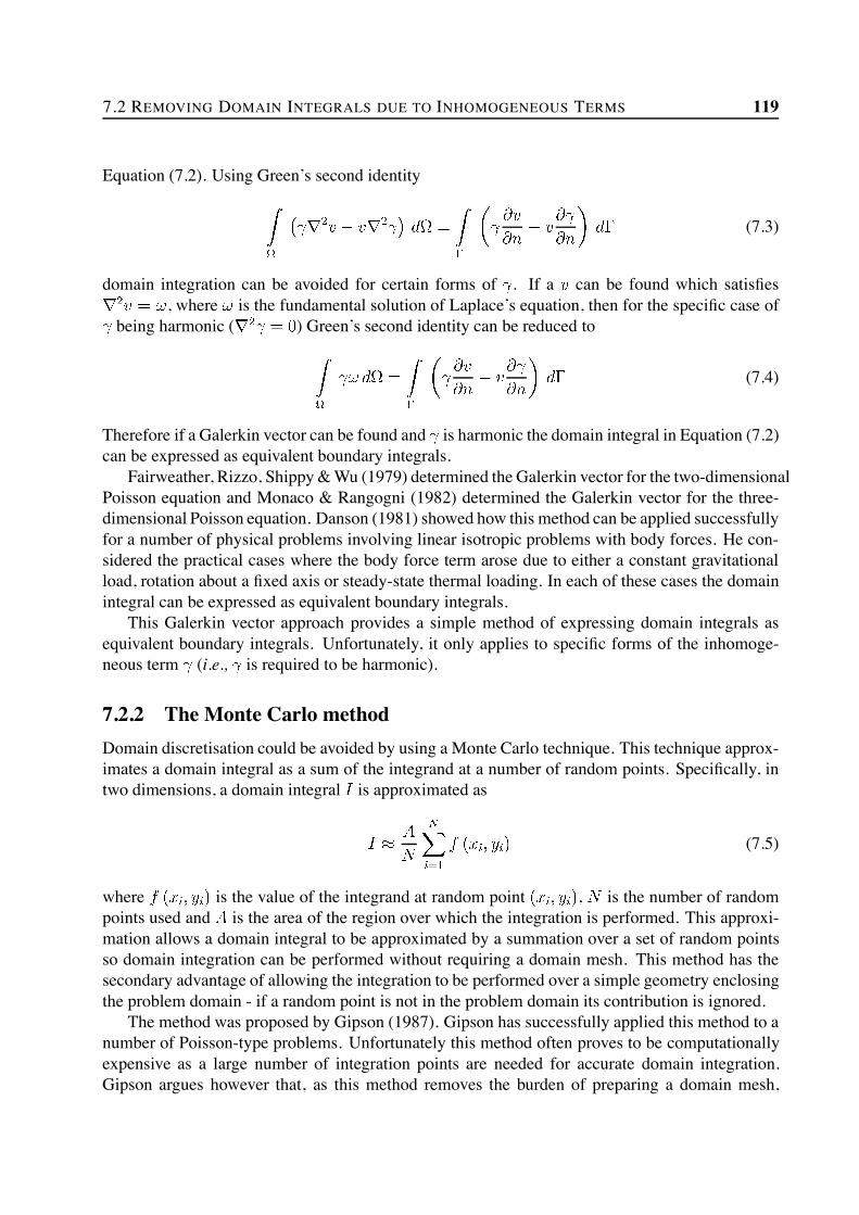
7.2 REMOVING DOMAIN INTEGRALS DUE TO INHOMOGENEOUS TERMS 119

Equation (7.2). Using Green’s second identity

(7.3)

domain integration can be avoided for certain forms of . If a can be found which satisfies, where is the fundamental solution of Laplace’s equation, then for the specific case of

being harmonic ( ) Green’s second identity can be reduced to

(7.4)

Therefore if a Galerkin vector can be found and is harmonic the domain integral in Equation (7.2)can be expressed as equivalent boundary integrals.

Fairweather, Rizzo, Shippy&Wu (1979) determined the Galerkin vector for the two-dimensionalPoisson equation and Monaco & Rangogni (1982) determined the Galerkin vector for the three-dimensional Poisson equation. Danson (1981) showed how this method can be applied successfullyfor a number of physical problems involving linear isotropic problems with body forces. He con-sidered the practical cases where the body force term arose due to either a constant gravitationalload, rotation about a fixed axis or steady-state thermal loading. In each of these cases the domainintegral can be expressed as equivalent boundary integrals.

This Galerkin vector approach provides a simple method of expressing domain integrals asequivalent boundary integrals. Unfortunately, it only applies to specific forms of the inhomoge-neous term (i.e., is required to be harmonic).

7.2.2 The Monte Carlo methodDomain discretisation could be avoided by using a Monte Carlo technique. This technique approx-imates a domain integral as a sum of the integrand at a number of random points. Specifically, intwo dimensions, a domain integral is approximated as

(7.5)

where is the value of the integrand at random point , is the number of randompoints used and is the area of the region over which the integration is performed. This approxi-mation allows a domain integral to be approximated by a summation over a set of random pointsso domain integration can be performed without requiring a domain mesh. This method has thesecondary advantage of allowing the integration to be performed over a simple geometry enclosingthe problem domain - if a random point is not in the problem domain its contribution is ignored.

The method was proposed by Gipson (1987). Gipson has successfully applied this method to anumber of Poisson-type problems. Unfortunately this method often proves to be computationallyexpensive as a large number of integration points are needed for accurate domain integration.Gipson argues however that, as this method removes the burden of preparing a domain mesh,


the extra computational expense is justified.

7.2.3 Complementary Function-Particular Integral methodA more general approach can be developed using particular solutions. Consider the linear problem

. can be considered as the sum of the complementary function , which is a solution ofthe homogeneous equation , and a particular solution which satisfies but isnot required to satisfy the boundary conditions of the problem. Applying BEM to the governingequation using the expansion gives

(7.6)

If a particular solution can be found, all values on the right-hand-side of Equation (7.6) areknown - reducing the problem to

(7.7)

where is a vector of known values. This linear system can be solved by applying boundaryconditions.

This approach can be applied in a situation where an analytic expression for a particular solu-tion can be found. Unfortunately particular solutions are generally only known for simple operatorsand for simple forms of . Alternatively an approximate particular solution could be calculated nu-merically. Zheng, Coleman & Phan-Thien (1991) proposed a method where a particular solutionis determined by approximating the inhomogeneous source term using a global interpolation func-tion. This approach is a special case of a more general method known as the dual reciprocityboundary element method.

7.3 Domain Integrals Involving the Dependent VariableConsider the linear homogeneous PDE . For many operators the fundamental solution tothe operator may be unobtainable or may be in an unusable form. This is especially likely ifinvolves variable coefficients for which case it has been shown that it is particularly difficult to finda fundamental solution. Instead, a BEM formulation can be derived based on a related operatorwith known fundamental solution. A BEM formulation for based on the operator willbe of the form

(7.8)

where is the fundamental solution corresponding to the operator . This integral equation issimilar to Equation (7.2). However in this case the domain integral term involves the dependentvariable . This problem could be solved using domain integration where the internal nodes aretreated as formal problem unknowns.

7.3 DOMAIN INTEGRALS INVOLVING THE DEPENDENT VARIABLE 121

7.3.1 The Perturbation Boundary Element MethodRangogni (1986) proposed solving variable coefficient PDEs by coupling the boundary elementmethod with a perturbation method. He considered the two-dimensional generalised Laplace equa-tion

(7.9)

Using the substitution Equation (7.9) can be recast as a heterogeneousHelmholtz equation

(7.10)

where is a known function of position.Rangogni treated this equation as a perturbation about Laplace’s equation. He considered the

class of equations

where (7.11)

for which he sought a solution of the form

(7.12)

Substituting Equation (7.12) into Equation (7.11) and grouping powers of gives

(7.13)

A solution will only exist for all values of if the terms at each power of equal zero. This allowsEquation (7.13) to be treated as an infinite series of distinct problems which can be solved usingthe boundary element method. can be found by solving which Rangogni assumeswill satisfy the boundary conditions of the original problem. Each successive can then be foundby solving a Poisson equation with homogeneous boundary conditions as has been previouslydetermined. Rangogni used a domain discretisation to solve these Poisson problems.

Equation (7.10) is a particular member of this family of equations for which . The

solution to Equation (7.10) is therefore given by . Rangogni reported that in practice this

series converged rapidly and in his numerical examples he achieved accurate results using onlyand .

Rangogni (1991) extended this coupled perturbation - boundary element method to the generalsecond-order variable coefficient PDE

(7.14)


He considered the family of equations

(7.15)

Applying the perturbation method to this family of equations allows Equation (7.15) to be ex-pressed as an infinite series of distinct Poisson equations which can be solved using the boundaryelement method. Again Rangogni used an domain mesh to solve these Poisson equations. Ran-gogni found that in practice convergence was rapid and accurate results were produced.

Gipson, Reible & Savant (1987) considered a class of hyperbolic and elliptic problems whichcan be transformed into an inhomogeneousHelmholtz equation. They used the perturbationmethodto recast this as an infinite sequence of Poisson equations. They avoided domain discretisation byusing a Monte Carlo integration technique (Gipson 1987) to evaluate the required domain integrals.

Lafe & Cheng (1987) used the perturbation method to solve steady-state groundwater flowproblems in heterogeneous aquifers. They showed the method produced accurate results for sim-ply varying hydraulic conductivities with convergence after two or three terms. Lafe & Chenginvestigated the convergence of the perturbation method. They found that for rapidly varying hy-draulic conductivity convergence is not guaranteed. From this investigation they concluded thataccurate results can be obtained so long as the hydraulic conductivity does not vary by more thanone order of magnitude within the solution domain. If the hydraulic conductivity variation is moresignificant they recommend using the perturbation method in conjunction with a subregion tech-nique so that the variation of conductivity within each subregion satisfies their requirements. Thisprocess could become computationally expensive, particularly if convergence is not rapid, as thesolution of multiple subproblems will be required within each subregion.

7.3.2 The Multiple Reciprocity MethodThe multiple reciprocity method (MRM) was initially proposed by Nowak (1987) for the solutionof transient heat conduction problems. Since then the method has been successfully applied to awide range of problems. The MRM can be viewed as a generalisation of the Galerkin vector ap-proach. Instead of using one higher-order fundamental solution, the Galerkin vector, to convert theremaining domain integrals to equivalent boundary integrals a series of higher-order fundamentalsolutions is used.

Consider the Poisson equation

(7.16)

where is a known function of position. Applying BEM to this equation, using thefundamental solution to the Laplace operator, gives

(7.17)

where is the known fundamental solution to Laplace’s equation applied at point . To avoiddomain discretisation the domain integral in Equation (7.17) needs to be expressed as equivalent


boundary integrals. Using MRM this is achieved by defining a higher-order fundamental solutionsuch that

(7.18)

Using this higher-order fundamental solution the domain integral in Equation (7.17) can be writtenas

(7.19)

or

(7.20)

This formulation has generated a new domain integral. is a known function so we can introducea new function which can be determined analytically from the relationship

(7.21)

giving

(7.22)

This process can be repeated by introducing a new higher-order fundamental solution such that

(7.23)

and continuing until convergence is reached.This procedure is based on the recurrence relationships

for (7.24)for (7.25)

Using these recurrence relationships gives the boundary integral formulation

(7.26)

which is an exact formulation if the infinite series converges. Errors are only introduced at thestage of boundary discretisation.


Introducing interpolattion functions and discretising the boundary gives the matrix system

(7.27)

where and are influence coefficient matrices corresponding to the higher-order fun-damental solutions and and contain the nodal values of and its normal derivative.

The MRM can be applied based on operators other than the Laplace operator. This approachrelies on knowledge of the higher-order fundamental solutions necessary for application of themethod. These solutions have been determined and successfully used for the Laplace operatorin both two and three dimensions but the extension of the method to other equation types needsfurther research. Itagaki & Brebbia (1993) have determined the higher order fundamental solutionsfor the two-dimensional modified Helmholtz equation.

TheMRM can be extended to other equations by allowing the forcing function to be a generalfunction such that . The MRM will be restricted to cases where the recurrencerelationships - Equations (7.24) and (7.25) - can be employed. Brebbia & Nowak (1989) haveapplied the MRM to the Helmholtz equation where and the recurrencerelationship defined by Equation (7.24) becomes simply

(7.28)

In this case the boundary integral formulation will be

(7.29)

7.3.3 The Dual Reciprocity Boundary Element MethodEquation Derivation

The dual reciprocity boundary element method (DR-BEM) was developed to avoid the need fordomain integration in cases where the fundamental solution of the governing differential equationis unknown or is impractical to apply. Instead the DR-BEM is applied using an appropriate relatedoperator with known fundamental solution. The most common choice is the Laplace operator(Partridge, Brebbia & Wrobel 1992) and in this chapter the DR-BEM will be illustrated for thischoice.

Consider a second-order PDE which can be expressed in the form

(7.30)

The forcing function can be completely general. If then is a known function of posi-tion and the differential equation described is simply the Poisson equation. For potential problems

and for transient problems . Applying the BEM to Equation (7.30) will


give

(7.31)

where is the known fundamental solution to Laplace’s equation. The aim of the DR-BEM is toexpress the domain integral due to the forcing function as equivalent boundary integrals.

The DR-BEM uses the idea of approximating using interpolation functions. A global approx-imation to of the form

(7.32)

is proposed. are unknown coefficients and are approximating functions used in the interpo-lation and are generally chosen to be functions of the source point and the field point of the fun-damental solution. The approximating functions are applied at different collocation points- called poles - generally most, but not all, of which are located on the boundary of the problemdomain.

As discussed in the previous chapter the solution to a linear PDE can be constructed asthe sum of a complimentary function (which satisfies the homogeneous equation ) and aparticular solution to the equation . Instead of using a single particular solution, whichmay be difficult to determine, the DR-BEM employs a series of particular solutions which arerelated to the approximating functions as shown in Equation (7.33).

(7.33)

By substituting Equations (7.32) and (7.33) into Equation (7.30) the forcing function is approxi-mated by a weighted summation of particular solutions to the Poisson equation.

(7.34)

The DR-BEM essentially constructs an approximate particular solution to the governing PDE as asummation of localised particular solutions.

With the governing equation rewritten in the form of Equation (7.34) the standard boundaryelement approach can be applied. Equation (7.34) is multiplied by a weighting function andintegrated over the domain. Green’s theorem is applied twice and the fundamental solution of theLaplacian is used to remove the remaining domain integrals. The name dual reciprocity BEM isderived from the application of reciprocity relationships to both sides of Equation (7.34). Afterapplying these steps Equation (7.35) is obtained, where the fundamental solution pole is applied at


point .

(7.35)

In implementing a numerical solution of this equation similar steps are taken as for the standardBEM. The boundary is discretised into elements and interpolation functions are introduced to ap-proximate the dependent variable within each element.

The form of each is known from Equation (7.33) once the approximating functions havebeen defined. It is not necessary to use interpolation functions to approximate each . Howeverby using the same interpolation functions to approximate and the numerical implementationwill generate the same matrices and on both sides of Equation (7.35). The error generatedby approximating each in this manner has been found to be small and can be justified by theimproved computational efficiency of the method (Partridge et al. 1992).

The application of this method results in the system

(7.36)

where the poles were chosen to be the boundary nodes plus internal points so that. Although it is not generally necessary to include poles at internal points it has been found

that in general improved accuracy is achieved by doing so (Nowak & Partridge 1992). It hasbeen shown that for many problems (Partridge et al. 1992) (Huang & Cruse 1993) using boundarypoints only in this procedure is insufficient to define the problem. In general using internal pointsis likely to improve the solution accuracy as it increases the number of degrees of freedom. Notheory has been developed of how many internal collocation points should be used for optimalaccuracy, or where these points should be positioned within the problem domain. Using internalpoles in this interpolation does not require domain discretisation - it is only necessary to specifythe coordinates of the internal collocation points. The internal points can be chosen to be locationswhere the solution is of interest.

The and vectors can be treated as columns of the matrices and respectively. Thisallows Equation (7.36) to be rewritten as

(7.37)

where is a vector containing the nodal values of . To solve this system it is necessary to evaluate. is defined by Equation (7.32) which, for the nodal values, can be expressed in matrix form as

. If the matrix is nonsingular this expression can be rearranged to give Equation (7.38)which provides an explicit expression for .

(7.38)


Including this explicit expression for in Equation (7.37) gives

(7.39)

The approach taken to solve this equation will depend on the form of .

The Approximating Function

The accuracy of the DR-BEM hinges on the accuracy of the global approximation to the forcingfunction (defined by Equation (7.32)). Therefore the choice of the approximating functions isa key consideration when implementing the DR-BEM. The only requirement so far prescribed onthe form of the approximating functions is that the matrix generated should be nonsingularand that the related particular solutions can be determined and can be expressed in a practicalclosed form. Some work has been conducted into investigating what form of should be used ina given situation to provide the highest accuracy and computational efficiency.

Usually a form of is defined and this can be used, applying Equation (7.33), to specifyand . The fundamental solution of Laplace’s equation is in two-dimensional

space and in three-dimensional space - where is the Euclidean distance betweenthe field point and the source point of the fundamental solution. Due to the dependence of thisfundamental solution only on the approximating function is generally chosen to be some radialfunction i.e., . Several other options for have been tried (Partridge et al. 1992) but ithas been found that in general the most accurate results were generated using some radial function.For both two and three-dimensional problems Wrobel, Brebbia & Nardini (1986) recommendedchoosing from the series

(7.40)

where is the distance between the field point (node ) and the DR-BEM collocation point (node). They showed that accurate results can be achieved using some combination of terms from thisseries. Generally the same approximating function is used at all the collocation points so in thisthesis, for simplicity, the form of approximating functions will be referred to by a single .

Choosing to be a function of only one variable simplifies the process of determining and .For two-dimensional problems, if then the relationship

(7.41)

can be reduced to the ordinary differential equation

(7.42)

Using defined by Equation (7.40) the corresponding forms of and , for two-dimensional


problems, can be shown to be

(7.43)

(7.44)

where and .Any combination of terms from Equation (7.40) can be used for specifying . It has been found

that in general including higher-order terms leads to little improvement in accuracy (Partridgeet al. 1992). The most commonly used form is as this approximation will generally giveaccurate results with greater computational efficiency than other choices.

Equation (7.40) was recommended as a basis for the approximating function due to theparticular form of the fundamental solution of Laplace’s equation and its dependence on only. Ifa different operator is used as the basis of the DR-BEM then it is likely a different form of willbe more appropriate. The choice of in this case will be discussed in Section 7.3.3.

The performance of the DR-BEM hinges on the choice of the approximating function . Thetheory of how to determine the best approximating function is therefore a vital component ofthe DR-BEM. Unfortunately the approximating function has generally been chosen and used in arather ad-hoc manner. Recently some more formal analysis of the use of approximating functionshas been undertaken.

Golberg & Chen (1994) argued that a formal analysis of the approximating function can beundertaken using the theory of radial basis functions. Radial basis functions are a generalisationof cubic splines in multi-dimensions. Cubic splines are known to be optimal for one-dimensionalinterpolation. Therefore, rather than being an arbitrary choice, it seems that choosing to bea radial function is a logical extension for two or three-dimensional problems. Golberg & Chenshowed that, for the Poisson equation, choosing to be a radial basis function ensures convergenceof the DR-BEM.

They also demonstrated that is a specific member of the group of radial basisfunctions. The theory of using radial basis functions for multi-dimensional approximation is fairlyadvanced. It has been shown that is optimal for three-dimensional problems which justifiesthe use of when applying the DR-BEM to three-dimensional problems - the constantis included to ensure a non-zero diagonal for . However for two-dimensional problems it hasbeen shown that optimal approximation is attained using the thin plate spline . Thisobservation lead Golberg & Chen to suggest that choosing to be a thin plate spline may improvethe accuracy of the DR-BEM in two dimensions. Recently Golberg (1995) has published a reviewof the DR-BEM concentrating on developments since 1990 concerning the numerical evaluationof particular solutions.

Inhomogeneous Equations

If the forcing function is a function of position only then the differential equation under consid-eration is simply Poisson’s equation. In this case it is not necessary to invert the matrix as cansimply be calculated from using Gaussian elimination. Equation (7.39) can be rewritten


as

where (7.45)

By applying boundary conditions Equation (7.45) can be reduced to a linear systemwhich can be solved to give the unknown nodal values of and .

Zheng et al. (1991) and Coleman, Tullock & Phan-Thien (1991) have proposed a method whichuses a global shape function to construct an approximate particular solution. As discussed byPolyzos, Dassios & Beskos (1994) this method is essentially equivalent to the DR-BEM. However,Zheng et al. and Coleman et al. suggested several alternative ways of determining the unknowncoefficients for inhomogeneous equations. Zheng et al. (1991) used a least-squares methodwhere they minimised the sum of squares

(7.46)

using singular value decomposition. For large systems they found the computational efficiencycould be improved by employing the conjugate gradient method. Coleman et al. (1991) success-fully solved inhomogeneous potential and elasticity problems which are governed by operatorsother than the Laplacian.

Elliptic Problems

If is a function of the dependent variable then will also be a function of the dependent variable.Consider, for example, the linear second-order differential equation

(7.47)

In this case so . Applying the DR-BEM to Equation (7.47), based on thefundamental solution to Laplace’s equation, gives

(7.48)

which can be rearranged to give

where (7.49)

Again, by applying boundary conditions Equation (7.49) can be reduced to a linear systemwhich can be solved to determine the unknown nodal values.Due to the presence of the fully-populated matrix in Equation (7.49) it is not possible to

solve the boundary problem and internal problem separately. Instead the solution can be treated asa coupled problem and the solutions at boundary and internal nodes are generated simultaneously.

Derivative Terms The DR-BEM can also be applied for elliptic problems where involvesderivatives of the dependent variable (Partridge et al. 1992). Consider, for example, the differ-


ential equation

(7.50)

In this case applying DR-BEM, using the Laplace fundamental solution, gives

(7.51)

To solve this problem it is necessary to relate the nodal values of to the nodal values of . Thisis achieved by using interpolation functions to approximate in a similar manner as was used toapproximate in Equation (7.32). A global approximation function of the form

(7.52)

can be used to approximate where are the chosen interpolation functions and are the un-known coefficients. In system form this can be expressed as

(7.53)

Although it is not necessary, equating to improves the computational efficiency of the methodas only one matrix inversion procedure is required. Differentiating Equation (7.53) gives

(7.54)

Choosing and inverting Equation (7.53) to give an explicit expression for allows Equa-tion (7.54) to be rewritten as

(7.55)

Equation (7.39) can now be rewritten as

where (7.56)

By applying boundary conditions Equation (7.56) can be reduced to a linear system which can besolved to give the unknown nodal values.

As mentioned earlier, the approximating function is generally chosen to be . Thiscan lead to numerical problems if derivative terms are included in the forcing function . As shownin Equation (7.55) derivative terms require derivatives of to be evaluated. For example, evaluating


the matrix requires calculation of . Using the approximating function gives

(7.57)

This derivative function can become singular, so - as shown by Zhang (1993) - significant numericalerror may result. This will especially be the case in problems where collocation points are locatedclose together.

Zhang (1993) suggested two possibilities for avoiding this problem. The first suggestion in-volved using a mapping procedure to map the governing equation to an equation without convec-tive terms. This method was shown to produce accurate results but is somewhat cumbersome andcan only be applied to linear problems. A simpler approach is to choose an approximating func-tion which does not lead to singularities for convective terms. Zhang recommended use of either

or . These approximating functions produce accurate results and can besimply applied for both linear and nonlinear problems. Zhang recommended the adoption of theseapproximating functions for all use of the DR-BEM.

The same idea of using Equation (7.53) to allow nodal values of to be associated to itsderivatives can be applied to extend the DR-BEM to cases involving higher-order derivatives orcross derivatives of the dependent variable. Appropriate approximating functions need to be chosento avoid the problem of singularities.

Variable Coefficients The DR-BEM can be readily extended to equations with variable coeffi-cients. Consider the variable coefficient Helmholtz equation

(7.58)

where is a function of position - in two dimensions. If the DR-BEM is applied usingthe known fundamental solution to the Laplace operator then the forcing function is .Applying the DR-BEM gives

(7.59)

where is a vector of the nodal values of the forcing function . The relationship can bewritten in matrix form as where is a diagonal matrix containing the nodal values of

i.e.,

... ... . . . ...(7.60)

where is the number of collocation points used in applying the DR-BEM.


Using this matrix expression for Equation (7.59) can be rearranged to give

where (7.61)

which is a boundary-only expression for the variable coefficient Helmholtz equation. This methodis general and can easily be extended to accommodate variable coefficient derivative terms and asum of variable coefficient terms.

Formulating the DR-BEM for a General Elliptic Problem In this section it has been shownhow the DR-BEM can be applied for elliptic problems with varying forms of . The DR-BEM canbe applied in cases where involves a sum of terms due to the basic property

(7.62)

Consider a two-dimensional equation of the form

(7.63)

Applying the DR-BEM to this equation gives a matrix system of the form

(7.64)

where

(7.65)

(7.66)

, and are diagonal matrices where the diagonals contain the nodal values of , andrespectively. is a vector containing the nodal values of .

The DR-BEM Using Other Operators

The DR-BEM has been presented in this chapter based on the Laplace operator. However the DR-BEM can be be applied using essentially any operator of appropriate order with known fundamentalsolution. If an appropriate operator can be found the complexity of the forcing function can bereduced. This should improve the accuracy of the method. The problem with applying the DR-BEM based on another operator is in choosing the approximating function . A choice of whichproduces accurate results is required but it is also necessary to choose an for which a particularsolution can be determined.


Zhu (1993) has determined the particular solutions necessary for applying the DR-BEM basedon the two-dimensional Helmholtz operator.

(7.67)

Radial functions have generally been used when applying the DR-BEM. Along the lines of Wrobelet al. (1986), Zhu chose an approximating function of the form where is a positiveinteger. Determining the particular solution requires solving the ordinary differential equation

(7.68)

which can be achieved using a variation of coefficients method.Partridge et al. (1992) applied the DR-BEM to the transient convection diffusion equation

(7.69)

where the material parameters , , and are all assumed to be homogeneous. They appliedthe DR-BEM based on the steady-state convection-diffusion operator

(7.70)

which has a known fundamental solution.This analysis requires the determination of a particular solution which satisfies

(7.71)

Instead of defining a form of the approximating function and solving for Partridge et al. choseto define and use Equation (7.71) to determine the corresponding approximating function. Al-though somewhat ad-hoc this approach was found to produce accurate results.

Chapter 8

The BEM for Parabolic PDES

8.1 Time-Stepping MethodsSeveral approaches have been proposed for applying the BEM to parabolic problems. These meth-ods can be broadly classified into two main approaches. Either some form of time-stepping proce-dure is used to advance the solution in time, or a semi-analytic technique is used which can directlycalculate a solution at a specified time. In this section time-stepping procedures will be considered.

Time-stepping approaches discretise the time domain in some manner and use some form oftime marching scheme to advance the solution from one discrete time to the next. The two mostcommonly used time-stepping methods are the coupled finite difference - BEM and the direct timeintegration method. These two methods will be outlined in this section for the diffusion equation

(8.1)

where the diffusivity is a material parameter which can be a constant or a function of position.

8.1.1 Coupled Finite Difference - Boundary Element MethodThis approach discretises the time-domain in a finite difference form. Consider the variation be-tween a time and a time . The most common approach (Brebbia et al. 1984b) isto assume that, for sufficiently small , the time derivative can be approximated using a first-orderfully implicit finite difference scheme

(8.2)

which allows the diffusion equation in this time-range to be approximated as

(8.3)

Using this finite difference approximation the original parabolic equation has been reduced to anelliptic equation. Using the weighted residuals method an integral equation can be generated from

136 THE BEM FOR PARABOLIC PDES

Equation (8.3).

(8.4)

where and . The fundamental solution is a solution of themodified Helmholtz equation

(8.5)

applied at some source point . The fundamental solution of the modified Helmholtz equationis known in both two and three dimensions. If an internal solution is required at a specific timethis can be determined explicitly from Equation (8.4) where the fundamental solution is applied atinternal point and .

Unfortunately Equation (8.4) contains a domain integral. This integral is generally evaluated byusing a domain mesh (Brebbia et al. 1984b). The domain integral does not include any problem un-knowns so a fairly coarse domain mesh will generally suffice. Applying the BEM to Equation (8.4)gives

(8.6)

where is a matrix containing the influence coefficients due to the domain integral. Using Equa-tion (8.6) the solution can be advanced in time. is known from the initial conditions so asolution can be calculated at . A solution at internal nodes can then be calculated. Thetime-stepping procedure can be repeated using the internal solution at as pseudo-initialconditions for the next time-step.

If a constant time-step is used the matrices , and can be calculated once and stored.The boundary conditions can be applied to form a solution system of the form where

is the vector of unknown nodal values at time and is a vector constructed fromknown nodal values from the previous time-step. For a problem with time-independent boundaryconditions at each time-step it is only necessary to update and solve the system for . If aproblem has time-dependent boundary conditions the solution system needs to be reformed at eachtime-step.

This coupled finite difference - boundary element method (FD-BEM) was first proposed byBrebbia & Walker (1980) for the diffusion equation. It was implemented and investigated byCurran, Cross & Lewis (1980). They found that this method will only produce accurate resultsif Equation (8.2) accurately approximates the time derivative. This will generally require smalltime-steps to be adopted. Curran et al. investigated the use of a higher-order approximation to thetime-derivative. They found that this improved the accuracy of the method. Unfortunately it leadto a deterioration in convergence behaviour.

Tanaka, Matsimoto&Yang (1994) proposed a generalised version of this time-stepping scheme.They approximated the time variation within an interval as

(8.7)

8.1 TIME-STEPPING METHODS 137

where , termed the time-scheme parameter, is a constant in the range . Substitutingthis approximation and a first-order finite difference approximation of the time derivative into thediffusion equation gives

(8.8)

If this approximation of the diffusion equation is equivalent to the standard FD-BEM dis-cussed earlier. An integral equation can be derived from Equation (8.8). Tanaka et al. implementedthis method and found it gave accurate results for a range of diffusion problems. They tested theaccuracy for a Crank-Nicolson scheme ( ), a Galerkin scheme ( ) and a fully implicitscheme ( ). They found that the best results were achieved using a Crank-Nicolson scheme.

8.1.2 Direct Time-Integration MethodInstead of converting the original parabolic equation to an elliptic equation the problem can betreated directly in the time domain by directly integrating over both time and space. The weightedresidual statement using this approach is

(8.9)

Integrating in time once and in space twice gives

(8.10)

where the fundamental solution satisfies

(8.11)

This time dependent fundamental solution is known in two and three dimensions. Physically thisfundamental solution represents the effect at a field point at time of a unit point source appliedat a point at time . If an internal solution is required at a specific time this can be determinedfrom Equation (8.10) with .

The variation of and with time is unknown so it is still necessary to step in time. However,as the time dependence is included in the fundamental solution, accurate results can be achievedusing larger time-steps than with the FD-BEM. Two different time-stepping schemes can be used.Similarly to the FD-BEM, each time-step can be treated as a new problem so that an internalsolution is constructed at the end of each time-step to be used as pseudo-initial conditions for thenext time-step. Alternatively the time integration process can be restarted at with increasingnumbers of intermediate steps used. These two time-stepping approaches are discussed in detail inBrebbia et al. (1984b).

The first method requires a new domain integral to be calculated after each time-step due to


the updated pseudo-initial conditions. The second time-stepping procedure involves only a domainintegral at so, ideally, a domain integral only needs to be calculated once. This, however, will stillrequire the user to create a domain mesh. As mentioned by Brebbia et al. (1984b), in many practicalcases the domain integral can be avoided. If the initial conditions are throughout the bodythe domain integral equals zero. If the initial conditions satisfy Laplace’s equation thena Galerkin vector can be found and the domain integral can be expressed as equivalent boundaryintegrals. This includes many practical cases such as constant initial temperature or an initial lineartemperature profile.

Unfortunately, in practice it is not always feasible to restart the integration process at . Ateach time-step new and matrices are required so if many time-steps are required the storagecapacity of the computer is likely to be exceeded. This requires the procedure to be restartedat some time where an internal solution is constructed and used as pseudo-initial conditions torepeat the process. Therefore, in practice, both time-stepping methods are likely to require domainintegration.

8.2 Laplace Transform MethodAn alternative approach which avoids time-stepping is to solve the problem in a transform domainwhich removes the time dependence of the problem. The parabolic PDE is thus converted to anelliptic problem for which the boundary element method has been shown to generally produceaccurate results. Once the solution to the elliptic problem is determined in the transform spacea solution in the original space can be attained using an inverse transform procedure. The mostappropriate transform approach for parabolic problems is the Laplace transform.

Consider the diffusion equation

(8.12)

with appropriate boundary and initial conditions. The Laplace transform of will be sym-bolised as and is defined as

(8.13)

Applying Laplace transforms to Equation (8.12) gives

(8.14)

with transformed boundary conditions. is the initial conditions of . Equation (8.14) is anelliptic PDE which can be readily solved using the boundary element method. Once the solutionis determined in Laplace transform space this solution can be inverted to give a solution in thetime-domain. This inversion procedure requires solutions to be generated for several values of thetransform parameter .

This method was first proposed by Rizzo & Shippy (1970) and has since been successfully

8.3 THE DR-BEM FOR TRANSIENT PROBLEMS 139

used by other practitioners (Moridis & Reddell 1991) (Zhu, Satravaha & Lu 1994). Liggett & Liu(1979) compared the Laplace transform method with the time-dependent Green’s function method.They noted that the direct method is simpler to apply. However, due to its greater efficiency, theyrecommended the Laplace transform method for solving diffusion problems.

One limitation of the Laplace transform method is that Equation (8.14) is inhomogeneous sothat applying the standard BEM will generate a domain integral involving the initial conditions.Traditionally this domain integral has been calculated by using a domain discretisation (Brebbiaet al. 1984b). However, recently Zhu et al. (1994) proposed using the DR-BEM to convert thisdomain integral term to equivalent boundary integrals. They chose to apply the DR-BEM basedon the known fundamental solution to the Laplace operator. Considering Equation (8.14) thismeans that the DR-BEM will be used to convert the right-hand-side to equivalent domain integrals.Therefore the required DR-BEM approximation is

(8.15)

The DR-BEM can now be applied to Equation (8.14), giving a matrix system of the form

(8.16)

which can be reduced to a square system by applying boundary conditions. Once the solutionis determined for this elliptic equation in the transform space a solution at a given time can beconstructed using an inversion process.

This Laplace transform dual reciprocity method (LT-DRM) can easily be extended to equationsof the form

(8.17)

in which case a matrix expression of the form

(8.18)

is generated. Zhu and his colleagues have successfully extended the LT-DRM to solve diffusionproblems with nonlinear source terms.

8.3 The DR-BEM For Transient ProblemsThe DR-BEM can also be applied to parabolic problems. Consider, for example, the diffusionequation

(8.19)


where the thermal diffusivity, , is a constant. In this case the global approximation of implies aseparation of variables such that

(8.20)

Using Equation (8.20), Equation (7.39) becomes

(8.21)

or

where (8.22)

Equation (8.22) can be solved using a standard direct time-integration method.Partridge & Brebbia (1990) recommended using a first-order finite difference approximation to

the time derivative

(8.23)

and linear approximations to and within a time-step.

(8.24)(8.25)

where and are weighting parameters with values in the range and the time-step isbetween times and . Substituting these approximations into Equation (8.22) anexpression at can be derived in terms of values at .

(8.26)

The values of and are known from the initial conditions so a time-stepping procedure can beused. If a constant time-step is used the matrices , and only need to be constructed once.Using this two-level time-integration scheme the most common choice of time-scheme parametersis .

8.4 The MRM for Transient Problems

The MRM can be applied to the diffusion equation using the fundamental solution

of Laplace’s equation. In this case the forcing function becomes and the recurrence

8.4 THE MRM FOR TRANSIENT PROBLEMS 141

relationship defined by Equation (7.24) becomes

(8.27)

The higher-order fundamental solutions are known for Laplace’s equation. In this case the MRMformulation becomes

(8.28)

The standard BEM numerical procedure can be applied to this boundary integral equation. Thisgives the matrix system

(8.29)

where the matrices etc are the influence coefficient matrices relating to the higher-orderfundamental solutions. This equation can be solved using a time-integration procedure.

The most common approach is to solve this system numerically by discretising the time domainand using a time-stepping procedure. This requires some interpolation between the two time-levelsmarked by and . This most common approach is to use a linear approximation to andin this time-range

(8.30)(8.31)

where has a value in the range 0 to 1. Differentiating these linear approximations gives

(8.32)

(8.33)

and all the other derivatives vanish.This allows Equation (8.29) to be simplified to

(8.34)

where , , ,

. This approach is termed a first-order approach as it removes all but thefirst derivatives. A second order approach can be formulated by using quadratic interpolation ofand within the time-range.

Using Equation (8.34) the solution can be advanced in time. If a constant time-step is used thematrices and only need to be constructed once outside the time-stepping loop.If the boundary conditions are not time-dependent the boundary conditions only need to be applied


once.

Bibliography

Brebbia, C. A. & Nowak, A. (1989), A new approach for transforming domain integrals to theboundary, in R. Gruber, J. Periaux & R. P. Shaw, eds, ’Proceedings of the Fifth InternationalSymposium on Numerical Methods in Engineering’, Computational Mechanics Publications,Springer-Verlag, pp. 73–84.

Brebbia, C. A., Telles, J. C. F. & Wrobel, L. C. (1984a), Boundary Element Techniques, Springer-Verlag.

Brebbia, C. A., Telles, J. C. F. & Wrobel, L. C. (1984b), Boundary element techniques: Theoryand applications in engineering, Springer-Verlag, New York.

Brebbia, C. A. & Walker, S. (1980), Boundary Element Techniques In Engineering, Newnes–Butterworths.

Clements, D. L. & Rizzo, F. (1978), ’A method for the numerical solution of boundary valueproblems governed by second-order elliptic systems’, Journal of the Institute of MathematicsApplications 22, 197–202.

Coleman, C. J., Tullock, D. L. & Phan-Thien, N. (1991), ’An effective boundary element methodfor inhomogeneous partial differential equations’, Journal of Applied Mathematics andPhysics (ZAMP) 42, 730–745.

Curran, D. A. S., Cross, M. & Lewis, B. A. (1980), ’Solution of parabolic differential equations bythe boundary element method using discretisation in time’, Applied Mathematical Modelling4, 398–400.

Danson, D. J. (1981), A boundary element formulation of problems in linear isotropic elasticitywith body forces, in C. A. Brebbia, ed., ’Boundary Element Methods’, Computational Me-chanics Publications and Springer-Verlag, pp. 105–122.

Fairweather, G., Rizzo, F. J., Shippy, D. J. & Wu, Y. S. (1979), ’On the numerical solution oftwo-dimensional problems by an improved boundary integral equation method’, J. Comput.Phys. 31, 96–112.

Gipson, G. S. (1987), Boundary Element Fundamentals - Basic Concepts And Recent Develop-ments In The Poisson Equation, Computational Mechanics Publications.

Gipson, G. S., Reible, D. D. & Savant, S. A. (1987), Boundary elements and perturbation theoryfor certain classes of hyperbolic and parabolic problems, in C. A. Brebbia, W. L. Wendland &

144 BIBLIOGRAPHY

G. Kuhn, eds, ’Boundary Elements IX’, ComputationalMechanics Publications and Springer-Verlag, pp. 115–127.

Golberg, M. A. (1995), ’The numerical evaluation of particular solutions in the BEM - a review’,Boundary Element Communications .

Golberg, M. A. & Chen, C. S. (1994), ’The theory of radial basis functions applied to the BEM forinhomogeneous partial differential equations’, BE Communications 5(2), 57–61.

Huang, Q. & Cruse, T. A. (1993), ’Some remarks on particular solution used in BEM formulation’,Computational Mechanics 13, 68–73.

Itagaki, M. & Brebbia, C. A. (1993), ’Generation of higher order fundamental solutions to the two-dimensional modified Helmholtz equation’, Engineering Analysis With Boundary Elements11(1), 87–90.

Lafe, O. E. & Cheng, A. H.-D. (1987), ’A perturbation boundary element code for steady stategroundwater flow in heterogeneous aquifers’, Water Resources Research 23(6), 1079–1084.

Liggett, J. A. & Liu, P. L.-F. (1979), ’Unsteady flow in confined aquifers: A comparison of twoboundary integral methods’,Water Resources Research 15(4), 861–866.

Monaco, A. D. & Rangogni, R. (1982), Boundary element method: Processing of the source termof the Poisson equation by means of boundary integrals only, in K. P. Holz, U. Meissner,W. Zielke, C. A. Brebbia, G. Pinder & W. Gray, eds, ’Finite Elements In Water ResourcesIV’, Springer-Verlag, pp. 19.29–19.36.

Moridis, G. L. & Reddell, D. L. (1991), The Laplace transform boundary element (LTBE) methodfor the solution of diffusion-type problems, in ’Boundary Elements XIII’, ComputationalMechanics Publications and Springer-Verlag, pp. 83–97.

Nowak, A. J. (1987), Solution of transient heat conduction problems using boundary-only formu-lation, in C. A. Brebbia, W. L. Wendland & G. Kuhn, eds, ’Boundary Elements IX Vol 3’,Computational Mechanics Publications and Springer-Verlag, pp. 265–276.

Nowak, A. J. & Partridge, P. W. (1992), ’Comparison of the dual reciprocity and the multiplereciprocity methods’, Engineering Analysis With Boundary Elements 10, 155–160.

Ortner, N. (1987), Construction of fundamental solutions, in C. A. Brebbia, ed., ’Topics In Bound-ary Elements Research’, Springer-Verlag, Berlin and New York.

Partridge, P. W. & Brebbia, C. A. (1990), The BEM dual reciprocity method for diffusion prob-lems, in ’Computational Methods In Water Resources VIII’, Computational Mechanics Pub-lications and Springer-Verlag, pp. 397–403.

Partridge, P. W., Brebbia, C. A. & Wrobel, L. C. (1992), The Dual Reciprocity Boundary ElementMethod, Computational Mechanics Publications and Elsevier Applied Science.

Polyzos, D., Dassios, G. & Beskos, D. E. (1994), ’On the equivalence of dual reciprocity andparticular integral approaches in the BEM’, BE Communications 5(6), 285–288.

BIBLIOGRAPHY 145

Rangogni, R. (1986), ’Numerical solution of the generalized Laplace equation by coupling theboundary element method and the perturbation method’, Applied Mathematical Modelling10, 266–270.

Rangogni, R. (1991), Solution of variable coefficients PDEs by means of BEM and perturba-tion technique, in ’Boundary Elements XIII’, Computational Mechanics Publications andSpringer-Verlag.

Rizzo, F. J. & Shippy, D. J. (1970), ’A method of solution for certain problems of heat conduction’,AIAA Journal 8(11), 2004–2009.

Tanaka, M., Matsimoto, T. & Yang, Q. F. (1994), ’Time-stepping boundary element method appliedto 2-D transient heat conduction problems’, Applied Mathematical Modelling 18, 569–576.

Wrobel, L. C., Brebbia, C. A. & Nardini, D. (1986), The dual reciprocity boundary element for-mulation for transient heat conduction, in ’Finite Elements In Water Resources VI’, Compu-tational Mechanics Publications and Springer-Verlag.

Wu, J. C. (1985), Boundary element methods and inhomogeneous parabolic equations, in C. A.Brebbia & B. J. Noye, eds, ’BETECH 85’, Springer-Verlag, pp. 19–30.

Zhang, Y. (1993), On the dual reciprocity boundary element method, Master’s thesis, The Univer-sity of Wollongong.

Zheng, R., Coleman, C. J. & Phan-Thien, N. (1991), ’A boundary element approach for non-homogeneous potential problems’, Computational Mechanics 7, 279–288.

Zhu, S. (1993), ’Particular solutions associated with the Helmholtz operator used in DRBEM’, BEAbstracts 4(6), 231–233.

Zhu, S., Satravaha, P. & Lu, X. (1994), ’Solving linear diffusion equations with the dual reciprocitymethod in Laplace space’, Engineering Analysis With Boundary Elements 13, 1–10.

Index

Advection-diffusion equation, 103Area Coordinates, 14

Basis functionsHermitecubic, 12

Basis functions, 2–16, 53Hermite, 10–14bicubic, 12, 14cubic, 10

Lagrange, 10bilinear, 7–9linear, 2–4quadratic, 7

Beam elements, 79Boundary conditions

application of, 29, 54

Coupled finite difference - boundary elementmethod, 135

Curvilinear coordinate systems, 17–19Cylindrical polar, 17Prolate spheroidal, 18Spherical polar, 18

Dirac-Delta function, 43–45Direct time-integration method, 137Dual reciprocity BEM

approximating function, 127derivative terms, 129elliptic problems, 129transient problems, 139variable coefficients, 131

Dual reciprocity BEM, 124, 133

element stiffness matrix, 26

Fundamental solution, 43, 45–48, 72, 117diffusion equation, 72

Helmholtz, 72Kelvin, 91Laplace, 46Navier, 72wave equation, 72

Galerkin formulation, 25, 31Galerkin vector, 119Gaussian quadrature, 39–42, 56Global stiffness matrix, 27

integration by parts, 24Isoparametric formulation, 53

Laplace transform method, 138

Mass lumping, 106Multiple reciprocity method, 122–124

diffusion equation, 140Helmholtz equation, 124Poisson equation, 122

Perturbation BEM, 121Plane stress elements, 81–83Potential energy, 82

Rayleigh-Ritz method, 75, 77Regular BEM, 64

Strain energy, 82

Trefftz method, 64Triangular elements, 14–16Truss elements, 76

Weighted residual, 24Weighting function, 24

Documents

Finite Element Method Boundary Element Method