Embed Size (px)
Citation preview
Delayed Mode QA/QC
Best Practice Manual
Version 3.0
April 2021
Version Date Comments Author
1.0 15/10/2018 Creation of document Mun Woo
2.0 21/08/2019 - Updated all ‘ANFOG’ to ‘IMOS Ocean Gliders’ or similar
- Corrected Figure 2 to reflect proper Slocum behaviour
- Incorporated Data Management info from ANFOG Data Management document
- Inserted Manual QC figures - Added section on Visualisation Tools - Updated Fig 1.
Mun Woo
2.1 7/11/2019 - Added multipoint calibration for Molar Oxygen
- Added WMO number as PLATFORM attribute
Mun Woo
2.2 10/3/2021 - Changed ‘salinity alignment’ to ‘temperature alignment’ in section 3.2.1.3 Conductivity alignment
- Updated Table 2. - Inserted missing word ‘cell’ in section
3.2.1.2.2.
Mun Woo
3.0 1/4/2021 - Added Stern/Volmer/Uchida formula for computation of dissolved oxygen concentration
- Added Claire Gourcuff to author list
Mun Woo
Citation
Woo, L.M. and Gourcuff, C. (2021). Delayed Mode QA/QC Best Practice Manual Version 3.0
Integrated Marine Observing System. DOI: 10.26198/5c997b5fdc9bd
(http://dx.doi.org/10.26198/5c997b5fdc9bd)
Contents 1 Introduction ........................................................................................................................................... 6
2 Background ............................................................................................................................................ 7
2.1 Gliders and sensor types................................................................................................................. 7
2.2 Known issues with sensors ............................................................................................................. 8
2.2.1 Sea-Bird CTD recorder............................................................................................................. 8
2.2.2 Examples of Slocum CTD data problems seen in IMOS data .................................................... 9
2.2.3 Aanderaa Optode ................................................................................................................. 11
2.2.4 Examples of Optode data problems seen in IMOS Slocum data ............................................. 14
2.2.5 Bio-optical Sensors ............................................................................................................... 17
2.2.6 Examples of bio-optical data problems seen in IMOS Slocum data ........................................ 18
3 Delayed-mode QA/QC .......................................................................................................................... 20
3.1 Glider data and metadata format ................................................................................................. 20
3.1.1 File name convention............................................................................................................ 21
3.1.2 Global attributes ................................................................................................................... 24
3.1.3 Metadata containers ............................................................................................................ 28
3.1.4 Dimensions ........................................................................................................................... 29
3.1.5 Variables............................................................................................................................... 30
3.1.6 Quality control flags .............................................................................................................. 36
3.2 Automated data corrections ......................................................................................................... 37
3.2.1 CTD corrections .................................................................................................................... 37
3.2.1.1 Temperature alignment .................................................................................................... 38
3.2.1.2 Thermal lag correction ...................................................................................................... 39
3.2.1.3 Conductivity alignment ..................................................................................................... 40
3.2.2 Oxygen Optode corrections .................................................................................................. 43
3.2.2.1 Geometrical alignment ..................................................................................................... 43
3.2.2.2 Time lag correction ........................................................................................................... 45
3.2.3 Bio-optical data corrections .................................................................................................. 48
4 Automatic Quality Tests ....................................................................................................................... 49
4.1 Impossible date test ..................................................................................................................... 49
4.2 Impossible location test ................................................................................................................ 49
4.3 Range test .................................................................................................................................... 49
4.4 Spike test ..................................................................................................................................... 50
4.5 Gradient test ................................................................................................................................ 50
4.6 Surface data ................................................................................................................................. 51
4.7 Descending IRRAD profiles............................................................................................................ 51
5 Manual Corrections.............................................................................................................................. 52
6 QC Reporting and File Submission ........................................................................................................ 55
7 Data Visualisation Tools ....................................................................................................................... 56
7.1 GLIDERSCOPE ............................................................................................................................... 56
7.2 NetCDF Ninja ................................................................................................................................ 58
Bibliography ................................................................................................................................................ 59
1 Introduction
This document is the IMOS Ocean Gliders (formerly known as Australian National Facility for Ocean
Gliders (ANFOG)) Best Practice manual for delayed mode processed data. IMOS Ocean Gliders is a
facility under Australia’s Integrated Marine Observing System (IMOS). IMOS Ocean Gliders, based in
the University of Western Australia (UWA), with IMOS National Collaborative Research Infrastructure
Strategy (NCRIS) funding, currently deploys a fleet of 11 gliders all around Australia, successfully
completing an average of 30 glider missions annually. The data retrieved from the glider fleet
contributes to the study of the major boundary current systems surrounding Australia and their links
to coastal ecosystem processes.
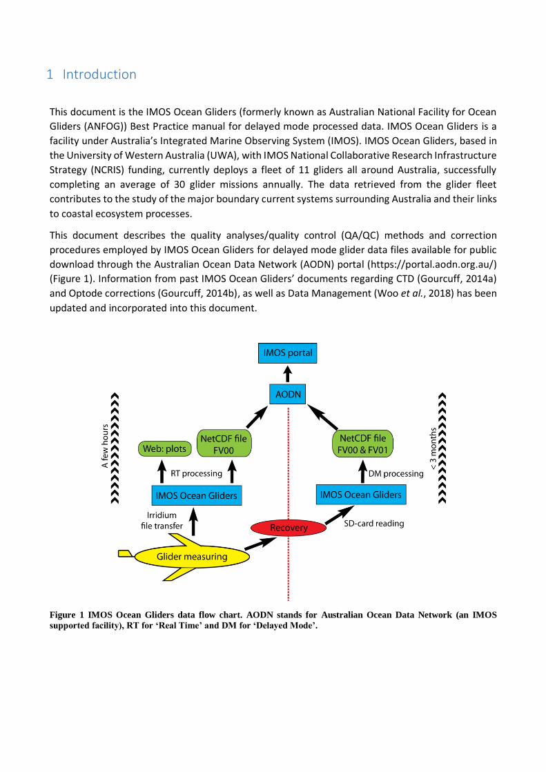
This document describes the quality analyses/quality control (QA/QC) methods and correction
procedures employed by IMOS Ocean Gliders for delayed mode glider data files available for public
download through the Australian Ocean Data Network (AODN) portal (https://portal.aodn.org.au/)
(Figure 1). Information from past IMOS Ocean Gliders’ documents regarding CTD (Gourcuff, 2014a)
and Optode corrections (Gourcuff, 2014b), as well as Data Management (Woo et al., 2018) has been
updated and incorporated into this document.
Figure 1 IMOS Ocean Gliders data flow chart. AODN stands for Australian Ocean Data Network (an IMOS
supported facility), RT for ‘Real Time’ and DM for ‘Delayed Mode’.
2 Background
2.1 Gliders and sensor types
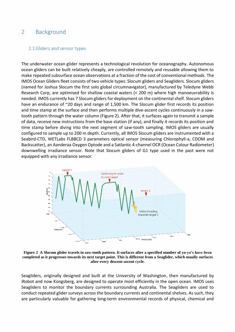
The underwater ocean glider represents a technological revolution for oceanography. Autonomous ocean gliders can be built relatively cheaply, are controlled remotely and reusable allowing them to make repeated subsurface ocean observations at a fraction of the cost of conventional methods. The IMOS Ocean Gliders fleet consists of two vehicle types: Slocum gliders and Seagliders. Slocum gliders (named for Joshua Slocum the first solo global circumnavigator), manufactured by Teledyne Webb Research Corp, are optimised for shallow coastal waters (< 200 m) where high manoeuvrability is needed. IMOS currently has 7 Slocum gliders for deployment on the continental shelf. Slocum gliders have an endurance of ~20 days and range of 1,500 km. The Slocum glider first records its position and time stamp at the surface and then performs multiple dive-ascent cycles continuously in a saw-tooth pattern through the water column (Figure 2). After that, it surfaces again to transmit a sample of data, receive new instructions from the base station (if any), and finally it records its position and time stamp before diving into the next segment of saw-tooth sampling. IMOS gliders are usually configured to sample up to 200 m depth. Currently, all IMOS Slocum gliders are instrumented with a Seabird-CTD, WETLabs FLBBCD 3 parameters optical sensor (measuring Chlorophyll-a, CDOM and Backscatter), an Aanderaa Oxygen Optode and a Satlantic 4-channel OCR (Ocean Colour Radiometer) downwelling irradiance sensor. Note that Slocum gliders of G1 type used in the past were not equipped with any irradiance sensor.
Figure 2 A Slocum glider travels in saw-tooth pattern. It surfaces after a specified number of yo-yo’s have been
completed as it progresses towards its next target point. This is different from a Seaglider, which usually surfaces
after every descent-ascent cycle.
Seagliders, originally designed and built at the University of Washington, then manufactured by iRobot and now Kongsberg, are designed to operate most efficiently in the open ocean. IMOS uses Seagliders to monitor the boundary currents surrounding Australia. The Seagliders are used to conduct repeated glider surveys across the boundary currents and continental shelves. As such, they are particularly valuable for gathering long-term environmental records of physical, chemical and
biological data. Seagliders have an endurance of 1-6 months, range of 6,000 km and can sample up to 1000 m depth. Typically, the Seaglider surfaces after every dive-ascent cycle, takes GPS fixes and sends data. On some occasions, pilots may set the Seaglider to surface after a pre-determined number of dives have been completed in order to navigate through strong surface currents. Unlike Slocum gliders for which only a subset of the dataset is transmitted while the glider is in the water (the full dataset will only be available for processing upon vehicle retrieval), Seagliders always send all their data at each surfacing. IMOS Seagliders are equipped with a Seabird-CTD, WETLabs BBFL2VMT 3 parameters optical sensor (measuring Chlorophyll-a, CDOM and Backscatter) and a Seabird Oxygen sensor.
2.2 Known issues with sensors
2.2.1 Sea-Bird CTD recorder
All gliders used at IMOS have been equipped with a Sea-Bird Conductivity Temperature Depth (CTD) recorder, optimized for low power consumption. Sea water salinity is computed using temperature, conductivity and pressure measurements acquired by this CTD. During the numerous IMOS Slocum missions performed to date, two types of CTD sensors have been used: the CTD41CP before June 2011 and the GPCTD thereafter. Both these instruments sample at a rate of ~0.5Hz. Their principal difference is that the CTD41CP was an un-pumped CTD, whereas the GPCTD, which has been specifically designed for Slocum gliders and are now installed on all current IMOS Slocum gliders, is equipped with a pump that allows for a constant flow inside the conductivity cell.
Sensor dynamics issues related to the typical profiling CTD, which were mainly high-frequency sampling CTD mounted on rosettes deployed from ships, have been described in the past (Horne and Toole (1980); Gregg and Hess (1985); Morison et al. (1994)). The issues usually manifest as spikes in salinity profiles as well as differences between a downward salinity profile and the following upward profile.
There are two main sources of data imperfections observed in salinity profiles: (i) different sensor time-responses of the thermistor, conductivity sensor and pressure sensor, and (ii) thermal lag effect. In the presence of differences in sensor time-responses, salinity is computed from pressure, conductivity and temperature measurement that don’t match up with one another. The thermal lag effect is due to conductivity cell inertia: the conductivity used to compute salinity is measured inside a conductivity cell, which has the capacity of storing heat. Thus, the temperature used to compute salinity does not accurately reflect the temperature of the ocean, especially when the glider is flying through strong temperature gradients. The thermal lag issue was shown to be much reduced when the glider CTD was pumped, so that the flushed water sample is supposedly the same as the water sampled by the thermistor (Janzen and Creed 2011). However, in practice, the issue is still present in data from pumped CTDs (see examples below), although more easily correctable as the flow in the conductivity cell is known and constant.
2.2.2 Examples of Slocum CTD data problems seen in IMOS data
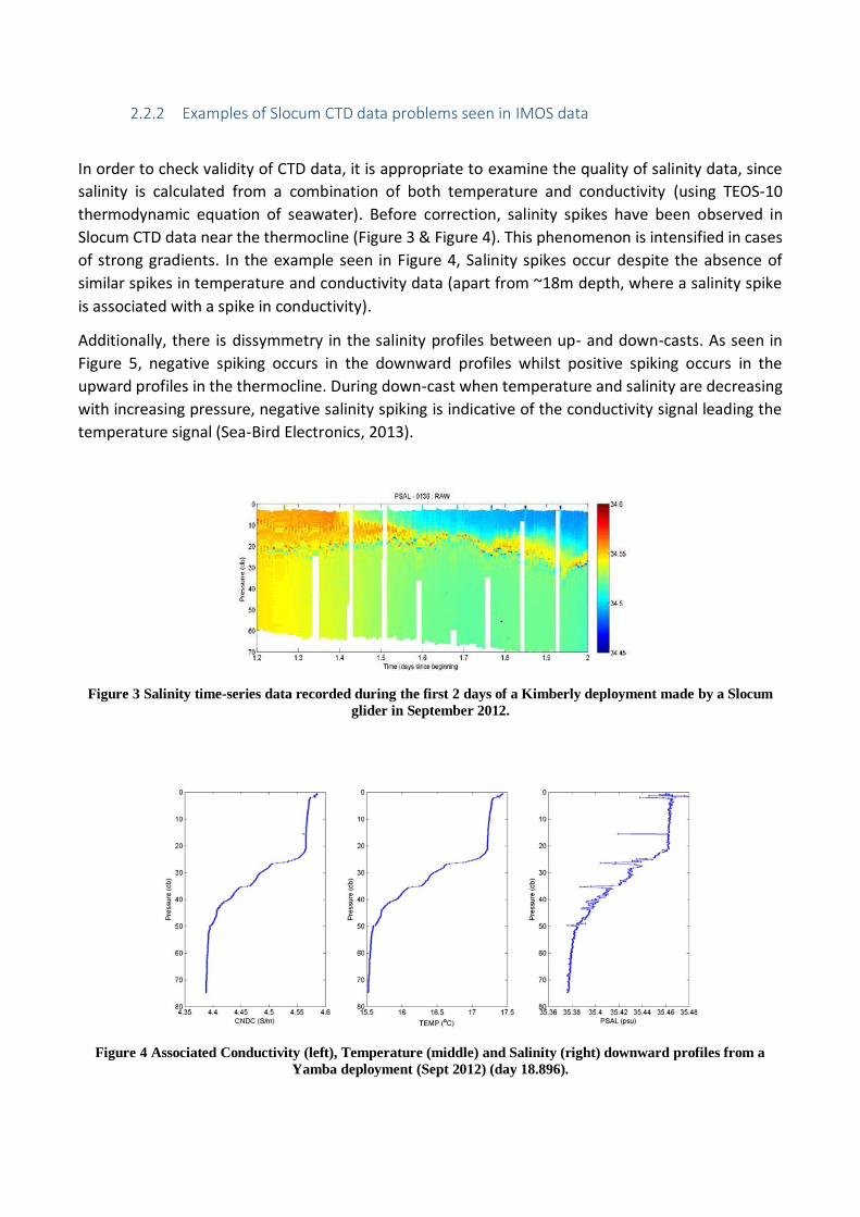
In order to check validity of CTD data, it is appropriate to examine the quality of salinity data, since
salinity is calculated from a combination of both temperature and conductivity (using TEOS-10
thermodynamic equation of seawater). Before correction, salinity spikes have been observed in
Slocum CTD data near the thermocline (Figure 3 & Figure 4). This phenomenon is intensified in cases
of strong gradients. In the example seen in Figure 4, Salinity spikes occur despite the absence of
similar spikes in temperature and conductivity data (apart from ~18m depth, where a salinity spike
is associated with a spike in conductivity).
Additionally, there is dissymmetry in the salinity profiles between up- and down-casts. As seen in
Figure 5, negative spiking occurs in the downward profiles whilst positive spiking occurs in the
upward profiles in the thermocline. During down-cast when temperature and salinity are decreasing
with increasing pressure, negative salinity spiking is indicative of the conductivity signal leading the
temperature signal (Sea-Bird Electronics, 2013).
Figure 3 Salinity time-series data recorded during the first 2 days of a Kimberly deployment made by a Slocum
glider in September 2012.
Figure 4 Associated Conductivity (left), Temperature (middle) and Salinity (right) downward profiles from a
Yamba deployment (Sept 2012) (day 18.896).
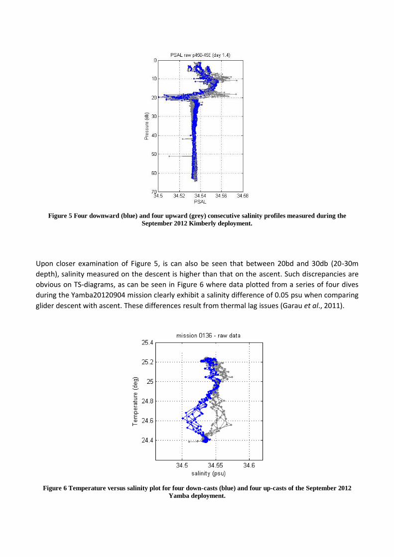
Figure 5 Four downward (blue) and four upward (grey) consecutive salinity profiles measured during the
September 2012 Kimberly deployment.
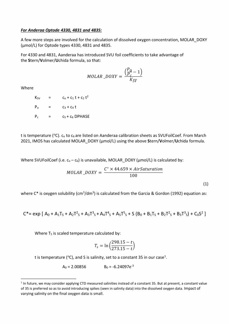
Upon closer examination of Figure 5, is can also be seen that between 20bd and 30db (20-30m
depth), salinity measured on the descent is higher than that on the ascent. Such discrepancies are
obvious on TS-diagrams, as can be seen in Figure 6 where data plotted from a series of four dives
during the Yamba20120904 mission clearly exhibit a salinity difference of 0.05 psu when comparing
glider descent with ascent. These differences result from thermal lag issues (Garau et al., 2011).
Figure 6 Temperature versus salinity plot for four down-casts (blue) and four up-casts of the September 2012
Yamba deployment.

2.2.3 Aanderaa Optode
IMOS Slocum gliders are equipped with Aanderaa Optodes (3835 – 5013W). The following is the
way in which the Optode internally computes dissolved oxygen concentration (in μmol/L).
Figure 7 Optode optical design (Aanderaa, 2007).
The uncalibrated phase measurement (UNCAL_PHASE) is calculated as the difference between
phase obtained with blue light excitation (BPHASE) and phase obtained with red light excitation
(RPHASE) (Aanderaa, 2007; Thierry et al., 2013):
UNCAL_PHASE = BPHASE – RPHASE
Since RPHASE is not used, it is set to zero.
Thus, UNCAL_PHASE= BPHASE
A calibrated phase (DPHASE) is calculated as a 3rd
degree polynomial of UNCAL_PHASE (or BPHASE, in our case):
𝐷𝑃𝐻𝐴𝑆𝐸 = 𝐴 + 𝐵 × 𝐵𝑃𝐻𝐴𝑆𝐸 + 𝐶 × 𝐵𝑃𝐻𝐴𝑆𝐸2 + 𝐷 × 𝐵𝑃𝐻𝐴𝑆𝐸3
where A, B, C and D are the PhaseCoef calibration coefficients (C and D are usually equal to zero).
For Anderaa Optode 3930, 3835, 3975, 4130 and 4175:
DPHASE is then converted to dissolved oxygen concentration, MOLAR_DOXY (μmol/L), using
additional foil-dependant coefficients in a 4th
degree polynomial:
𝑀𝑂𝐿𝐴𝑅 _𝐷𝑂𝑋𝑌 = 𝐶0 + 𝐶1 × 𝐷𝑃𝐻𝐴𝑆𝐸 + 𝐶2 × 𝐷𝑃𝐻𝐴𝑆𝐸2 + 𝐶3 × 𝐷𝑃𝐻𝐴𝑆𝐸3 + 𝐶4 × 𝐷𝑃𝐻𝐴𝑆𝐸4
where C0, C1, C2, C3, C4 are temperature dependant coefficients calculated as:
𝐶𝑖 = 𝐶𝑖0 + 𝐶𝑖1 × 𝑇 + 𝐶𝑖2 × 𝑇2 + 𝐶𝑖3 × 𝑇3
T is temperature (°C), and Cij are 20 foil-dependant calibration coefficients. One set of these 20 calibration coefficients is associated with each batch of foils.
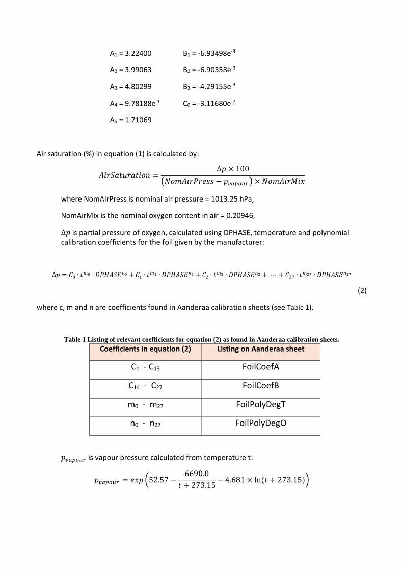
For Anderaa Optode 4330, 4831 and 4835:
A few more steps are involved for the calculation of dissolved oxygen concentration, MOLAR_DOXY (μmol/L) for Optode types 4330, 4831 and 4835.
For 4330 and 4831, Aanderaa has introduced SVU foil coefficients to take advantage of the Stern/Volmer/Uchida formula, so that:
𝑀𝑂𝐿𝐴𝑅 _𝐷𝑂𝑋𝑌 = (
𝑃o𝑃𝑐
− 1)
𝐾𝑆𝑉
Where
KSV = co + c1 t + c2 t2
Po = c3 + c4 t
Pc = c5 + c6 DPHASE
t is temperature (oC). co to c6 are listed on Aanderaa calibration sheets as SVUFoilCoef. From March 2021, IMOS has calculated MOLAR_DOXY (μmol/L) using the above Stern/Volmer/Uchida formula.
Where SVUFoilCoef (i.e. co – c6) is unavailable, MOLAR_DOXY (μmol/L) is calculated by:
𝑀𝑂𝐿𝐴𝑅 _𝐷𝑂𝑋𝑌 = 𝐶∗ × 44.659 × 𝐴𝑖𝑟𝑆𝑎𝑡𝑢𝑟𝑎𝑡𝑖𝑜𝑛
100
(1)
where C* is oxygen solubility (cm3/dm3) is calculated from the Garcia & Gordon (1992) equation as:
C*= exp [ A0 + A1TS + A2T2S + A3T3
S + A4T4S + A5T5
S + S (B0 + B1TS + B2T2S + B3T3
S) + C0S2 ]
Where TS is scaled temperature calculated by:
𝑇𝑠 = ln (298.15 − 𝑡
273.15 − 𝑡)
t is temperature (oC), and S is salinity, set to a constant 35 in our case1.
A0 = 2.00856 B0 = -6.24097e-3
1 In future, we may consider applying CTD measured salinities instead of a constant 35. But at present, a constant value
of 35 is preferred so as to avoid introducing spikes (seen in salinity data) into the dissolved oxygen data. Impact of varying salinity on the final oxygen data is small.
A1 = 3.22400 B1 = -6.93498e-3
A2 = 3.99063 B2 = -6.90358e-3
A3 = 4.80299 B3 = -4.29155e-3
A4 = 9.78188e-1 C0 = -3.11680e-7
A5 = 1.71069
Air saturation (%) in equation (1) is calculated by:
𝐴𝑖𝑟𝑆𝑎𝑡𝑢𝑟𝑎𝑡𝑖𝑜𝑛 =∆𝑝 × 100
(𝑁𝑜𝑚𝐴𝑖𝑟𝑃𝑟𝑒𝑠𝑠 − 𝑝𝑣𝑎𝑝𝑜𝑢𝑟 ) × 𝑁𝑜𝑚𝐴𝑖𝑟𝑀𝑖𝑥
where NomAirPress is nominal air pressure = 1013.25 hPa,
NomAirMix is the nominal oxygen content in air = 0.20946,
∆𝑝 is partial pressure of oxygen, calculated using DPHASE, temperature and polynomial calibration coefficients for the foil given by the manufacturer:
∆𝑝 = 𝐶0 ∙ 𝑡𝑚0 ∙ 𝐷𝑃𝐻𝐴𝑆𝐸𝑛0 + 𝐶1 ∙ 𝑡𝑚1 ∙ 𝐷𝑃𝐻𝐴𝑆𝐸𝑛1 + 𝐶2 ∙ 𝑡𝑚2 ∙ 𝐷𝑃𝐻𝐴𝑆𝐸𝑛2 + ⋯ + 𝐶27 ∙ 𝑡𝑚27 ∙ 𝐷𝑃𝐻𝐴𝑆𝐸𝑛27
(2)
where c, m and n are coefficients found in Aanderaa calibration sheets (see Table 1).
Table 1 Listing of relevant coefficients for equation (2) as found in Aanderaa calibration sheets.
Coefficients in equation (2) Listing on Aanderaa sheet
Co - C13 FoilCoefA
C14 - C27 FoilCoefB
m0 - m27 FoilPolyDegT
n0 - n27 FoilPolyDegO
𝑝𝑣𝑎𝑝𝑜𝑢𝑟 is vapour pressure calculated from temperature t:
𝑝𝑣𝑎𝑝𝑜𝑢𝑟 = 𝑒𝑥𝑝 (52.57 −6690.0
𝑡 + 273.15− 4.681 × ln (𝑡 + 273.15))
Thereafter, multipoint calibration is applied using additional ConcCoef_0 and ConcCoef_1 values found in Aanderaa calibration sheets, such that
MOLAR_DOXYcorrected = MOLAR_DOXY × (ConcCoef1) + ConcCoef0
Salinity compensation:
The dissolved oxygen concentration is also corrected for salinity effects. Salinity compensated MOLAR_DOXY is finally calculated as:
MOLAR_DOXYSAL-compensated
= MOLAR_DOXY * exp [ (Sset
) (B0
+ B1T
S + B
2T
S
2 + B
3T
S
3) + C
0*(S
set
2)]
where Sset=35, in our case.
Early IMOS Slocum deployments were performed with the glider configured such that only the
internally computed dissolved oxygen data in μmol/L were recorded. However, from May/June 2011,
glider configuration settings were changed to “wphase” (sci_oxy3835_wphase_is_installed
=1), allowing outputs of many more parameters. Thus, for deployments performed since mid-2011,
the BPHASE, DPHASE and Optode temperature measurements have also become available. This is of
critical importance for the improvement of oxygen data quality, as described in section 3.2.2.
2.2.4 Examples of Optode data problems seen in IMOS Slocum data
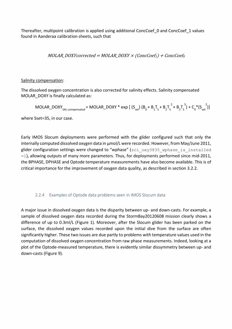
A major issue in dissolved oxygen data is the disparity between up- and down-casts. For example, a
sample of dissolved oxygen data recorded during the StormBay20120608 mission clearly shows a
difference of up to 0.3ml/L (Figure 1). Moreover, after the Slocum glider has been parked on the
surface, the dissolved oxygen values recorded upon the initial dive from the surface are often
significantly higher. These two issues are due partly to problems with temperature values used in the
computation of dissolved oxygen concentration from raw phase measurements. Indeed, looking at a
plot of the Optode-measured temperature, there is evidently similar dissymmetry between up- and
down-casts (Figure 9).
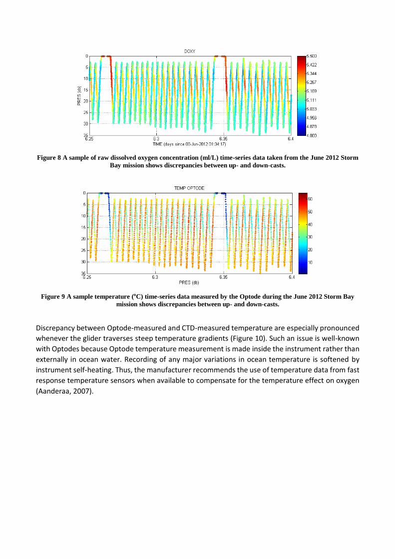
Figure 8 A sample of raw dissolved oxygen concentration (ml/L) time-series data taken from the June 2012 Storm
Bay mission shows discrepancies between up- and down-casts.
Figure 9 A sample temperature (oC) time-series data measured by the Optode during the June 2012 Storm Bay
mission shows discrepancies between up- and down-casts.
Discrepancy between Optode-measured and CTD-measured temperature are especially pronounced
whenever the glider traverses steep temperature gradients (Figure 10). Such an issue is well-known
with Optodes because Optode temperature measurement is made inside the instrument rather than
externally in ocean water. Recording of any major variations in ocean temperature is softened by
instrument self-heating. Thus, the manufacturer recommends the use of temperature data from fast
response temperature sensors when available to compensate for the temperature effect on oxygen
(Aanderaa, 2007).
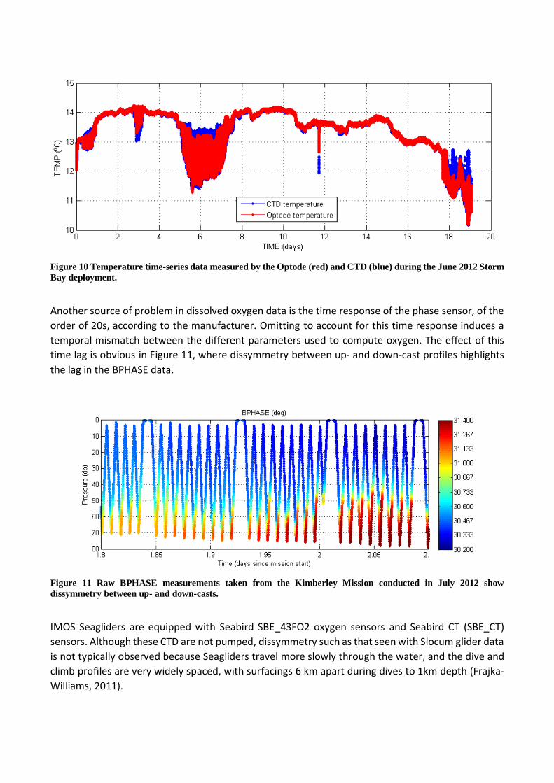
Figure 10 Temperature time-series data measured by the Optode (red) and CTD (blue) during the June 2012 Storm
Bay deployment.
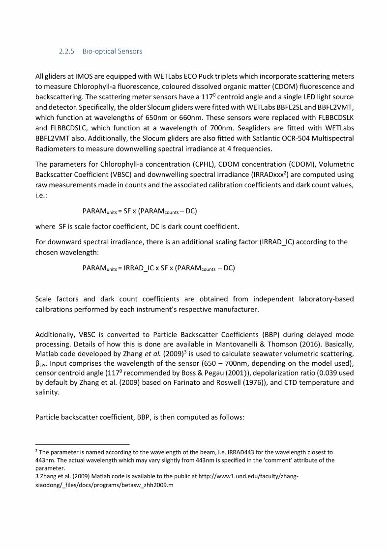
Another source of problem in dissolved oxygen data is the time response of the phase sensor, of the
order of 20s, according to the manufacturer. Omitting to account for this time response induces a
temporal mismatch between the different parameters used to compute oxygen. The effect of this
time lag is obvious in Figure 11, where dissymmetry between up- and down-cast profiles highlights
the lag in the BPHASE data.
Figure 11 Raw BPHASE measurements taken from the Kimberley Mission conducted in July 2012 show
dissymmetry between up- and down-casts.
IMOS Seagliders are equipped with Seabird SBE_43FO2 oxygen sensors and Seabird CT (SBE_CT)
sensors. Although these CTD are not pumped, dissymmetry such as that seen with Slocum glider data
is not typically observed because Seagliders travel more slowly through the water, and the dive and
climb profiles are very widely spaced, with surfacings 6 km apart during dives to 1km depth (Frajka-
Williams, 2011).
2.2.5 Bio-optical Sensors
All gliders at IMOS are equipped with WETLabs ECO Puck triplets which incorporate scattering meters
to measure Chlorophyll-a fluorescence, coloured dissolved organic matter (CDOM) fluorescence and
backscattering. The scattering meter sensors have a 1170 centroid angle and a single LED light source
and detector. Specifically, the older Slocum gliders were fitted with WETLabs BBFL2SL and BBFL2VMT,
which function at wavelengths of 650nm or 660nm. These sensors were replaced with FLBBCDSLK
and FLBBCDSLC, which function at a wavelength of 700nm. Seagliders are fitted with WETLabs
BBFL2VMT also. Additionally, the Slocum gliders are also fitted with Satlantic OCR-504 Multispectral
Radiometers to measure downwelling spectral irradiance at 4 frequencies.
The parameters for Chlorophyll-a concentration (CPHL), CDOM concentration (CDOM), Volumetric
Backscatter Coefficient (VBSC) and downwelling spectral irradiance (IRRADxxx2) are computed using
raw measurements made in counts and the associated calibration coefficients and dark count values,
i.e.:
PARAMunits = SF x (PARAMcounts – DC)
where SF is scale factor coefficient, DC is dark count coefficient.
For downward spectral irradiance, there is an additional scaling factor (IRRAD_IC) according to the
chosen wavelength:
PARAMunits = IRRAD_IC x SF x (PARAMcounts – DC)
Scale factors and dark count coefficients are obtained from independent laboratory-based
calibrations performed by each instrument’s respective manufacturer.
Additionally, VBSC is converted to Particle Backscatter Coefficients (BBP) during delayed mode processing. Details of how this is done are available in Mantovanelli & Thomson (2016). Basically, Matlab code developed by Zhang et al. (2009)3 is used to calculate seawater volumetric scattering, βsw. Input comprises the wavelength of the sensor (650 – 700nm, depending on the model used), censor centroid angle (1170 recommended by Boss & Pegau (2001)), depolarization ratio (0.039 used by default by Zhang et al. (2009) based on Farinato and Roswell (1976)), and CTD temperature and salinity.
Particle backscatter coefficient, BBP, is then computed as follows:
2 The parameter is named according to the wavelength of the beam, i.e. IRRAD443 for the wavelength closest to 443nm. The actual wavelength which may vary slightly from 443nm is specified in the ‘comment’ attribute of the parameter. 3 Zhang et al. (2009) Matlab code is available to the public at http://www1.und.edu/faculty/zhang-
xiaodong/_files/docs/programs/betasw_zhh2009.m
𝐵𝐵𝑃 = 2𝜋 × (𝑉𝐵𝑆𝐶 − 𝛽𝑠𝑤) × 𝑋𝑝
where Xp = 1.1 (recommended by WETLabs 2013)
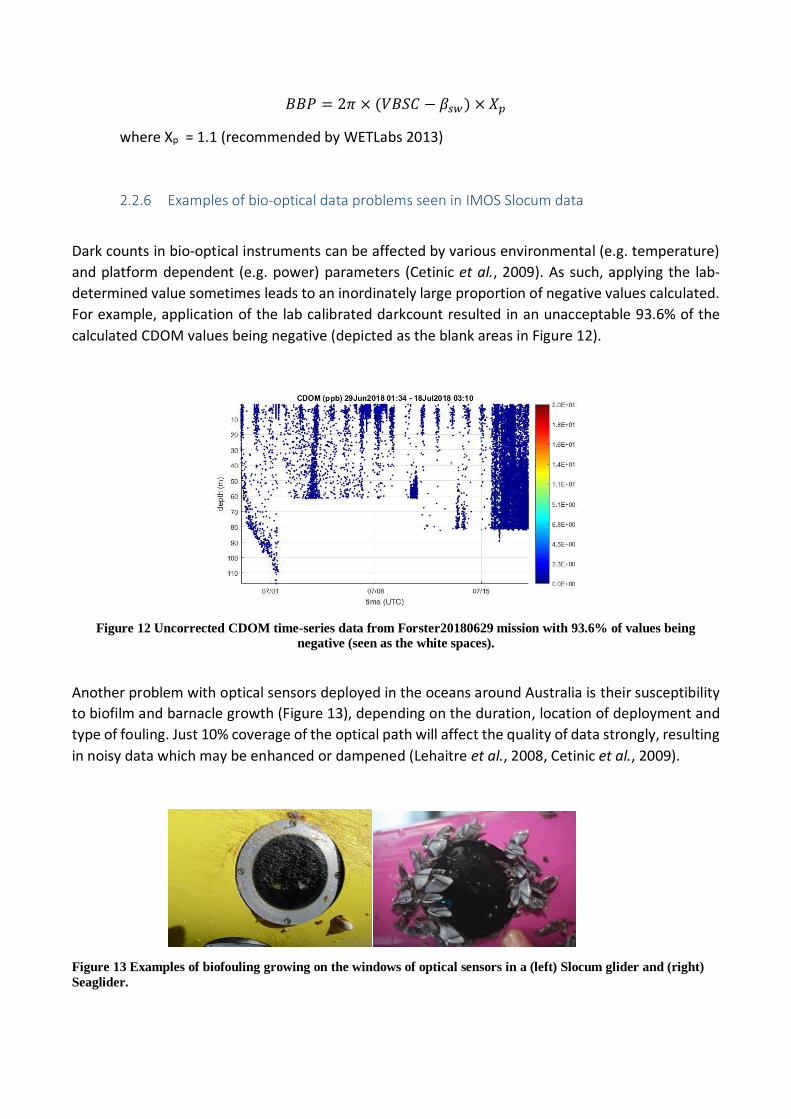
2.2.6 Examples of bio-optical data problems seen in IMOS Slocum data
Dark counts in bio-optical instruments can be affected by various environmental (e.g. temperature)
and platform dependent (e.g. power) parameters (Cetinic et al., 2009). As such, applying the lab-
determined value sometimes leads to an inordinately large proportion of negative values calculated.
For example, application of the lab calibrated darkcount resulted in an unacceptable 93.6% of the
calculated CDOM values being negative (depicted as the blank areas in Figure 12).
Figure 12 Uncorrected CDOM time-series data from Forster20180629 mission with 93.6% of values being
negative (seen as the white spaces).
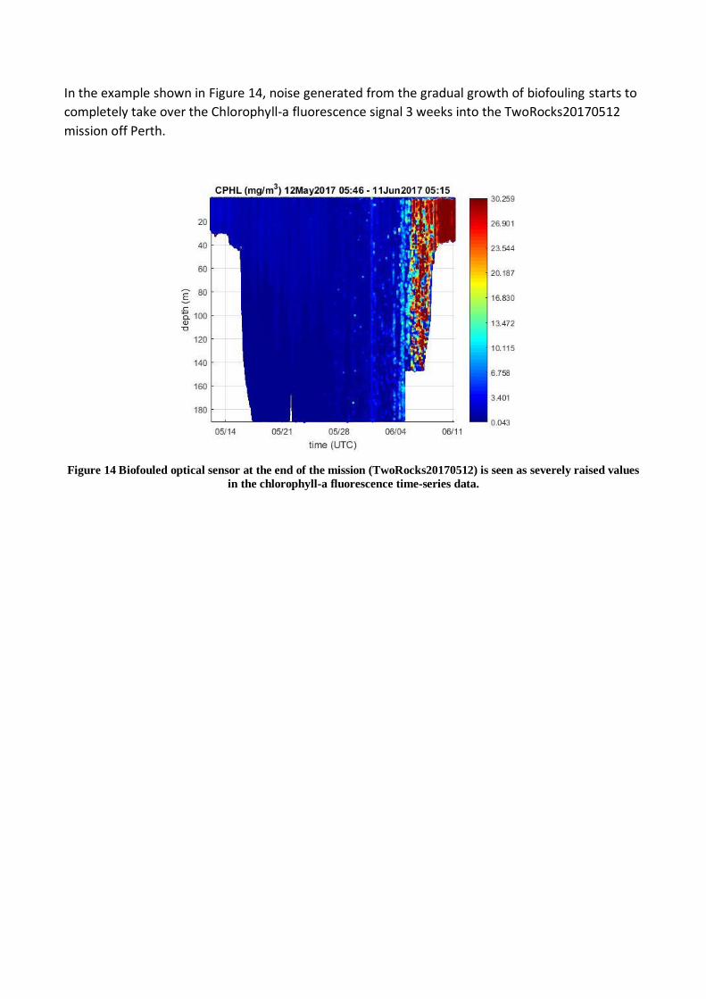
Another problem with optical sensors deployed in the oceans around Australia is their susceptibility
to biofilm and barnacle growth (Figure 13), depending on the duration, location of deployment and
type of fouling. Just 10% coverage of the optical path will affect the quality of data strongly, resulting
in noisy data which may be enhanced or dampened (Lehaitre et al., 2008, Cetinic et al., 2009).
Figure 13 Examples of biofouling growing on the windows of optical sensors in a (left) Slocum glider and (right)
Seaglider.
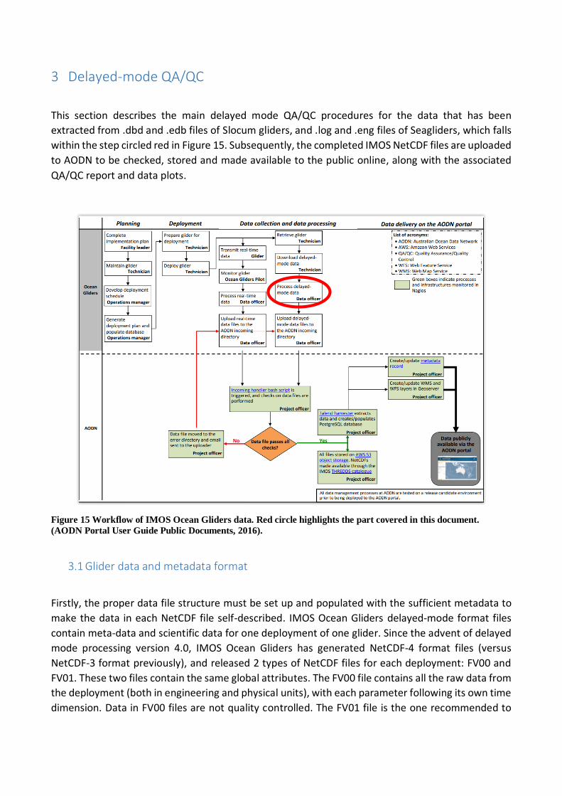
In the example shown in Figure 14, noise generated from the gradual growth of biofouling starts to
completely take over the Chlorophyll-a fluorescence signal 3 weeks into the TwoRocks20170512
mission off Perth.
Figure 14 Biofouled optical sensor at the end of the mission (TwoRocks20170512) is seen as severely raised values
in the chlorophyll-a fluorescence time-series data.
3 Delayed-mode QA/QC
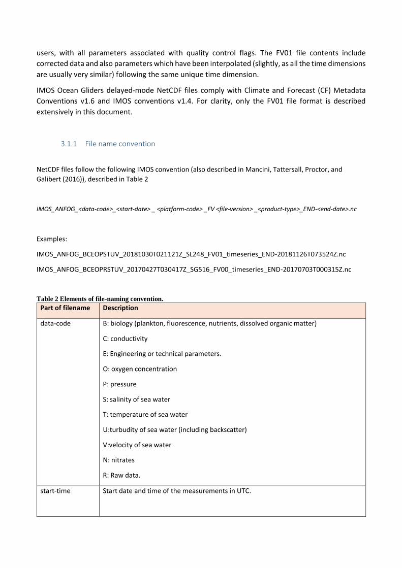
This section describes the main delayed mode QA/QC procedures for the data that has been
extracted from .dbd and .edb files of Slocum gliders, and .log and .eng files of Seagliders, which falls
within the step circled red in Figure 15. Subsequently, the completed IMOS NetCDF files are uploaded
to AODN to be checked, stored and made available to the public online, along with the associated
QA/QC report and data plots.
Figure 15 Workflow of IMOS Ocean Gliders data. Red circle highlights the part covered in this document.
(AODN Portal User Guide Public Documents, 2016).
3.1 Glider data and metadata format
Firstly, the proper data file structure must be set up and populated with the sufficient metadata to
make the data in each NetCDF file self-described. IMOS Ocean Gliders delayed-mode format files
contain meta-data and scientific data for one deployment of one glider. Since the advent of delayed
mode processing version 4.0, IMOS Ocean Gliders has generated NetCDF-4 format files (versus
NetCDF-3 format previously), and released 2 types of NetCDF files for each deployment: FV00 and
FV01. These two files contain the same global attributes. The FV00 file contains all the raw data from
the deployment (both in engineering and physical units), with each parameter following its own time
dimension. Data in FV00 files are not quality controlled. The FV01 file is the one recommended to
users, with all parameters associated with quality control flags. The FV01 file contents include
corrected data and also parameters which have been interpolated (slightly, as all the time dimensions
are usually very similar) following the same unique time dimension.
IMOS Ocean Gliders delayed-mode NetCDF files comply with Climate and Forecast (CF) Metadata
Conventions v1.6 and IMOS conventions v1.4. For clarity, only the FV01 file format is described
extensively in this document.
3.1.1 File name convention
NetCDF files follow the following IMOS convention (also described in Mancini, Tattersall, Proctor, and
Galibert (2016)), described in Table 2
IMOS_ANFOG_<data-code>_<start-date> _ <platform-code> _FV <file-version> _<product-type>_END-<end-date>.nc
Examples:
IMOS_ANFOG_BCEOPSTUV_20181030T021121Z_SL248_FV01_timeseries_END-20181126T073524Z.nc
IMOS_ANFOG_BCEOPRSTUV_20170427T030417Z_SG516_FV00_timeseries_END-20170703T000315Z.nc
Table 2 Elements of file-naming convention.
Part of filename Description
data-code B: biology (plankton, fluorescence, nutrients, dissolved organic matter)
C: conductivity
E: Engineering or technical parameters.
O: oxygen concentration
P: pressure
S: salinity of sea water
T: temperature of sea water
U:turbudity of sea water (including backscatter)
V:velocity of sea water
N: nitrates
R: Raw data.
start-time Start date and time of the measurements in UTC.
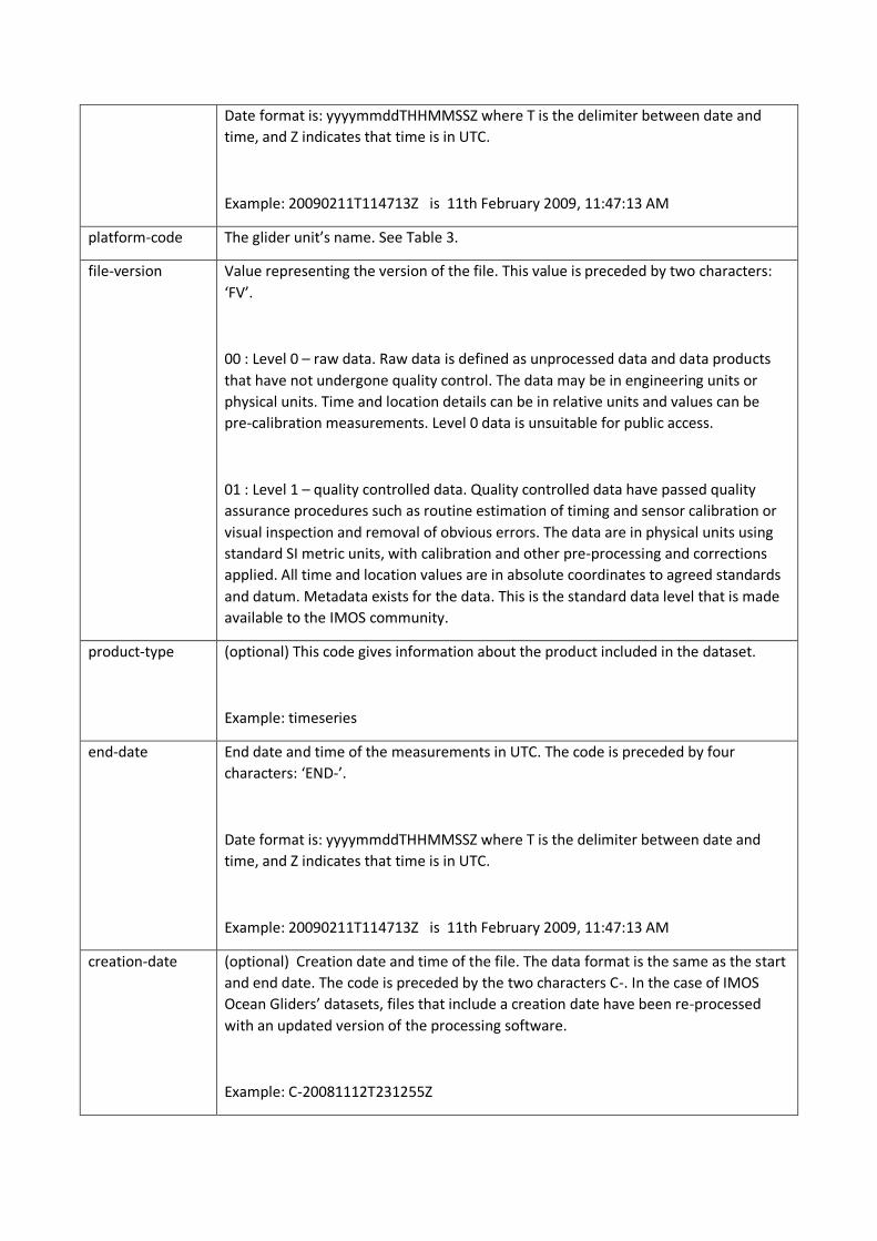
Date format is: yyyymmddTHHMMSSZ where T is the delimiter between date and
time, and Z indicates that time is in UTC.
Example: 20090211T114713Z is 11th February 2009, 11:47:13 AM
platform-code The glider unit’s name. See Table 3.
file-version Value representing the version of the file. This value is preceded by two characters:
‘FV’.
00 : Level 0 – raw data. Raw data is defined as unprocessed data and data products
that have not undergone quality control. The data may be in engineering units or
physical units. Time and location details can be in relative units and values can be
pre-calibration measurements. Level 0 data is unsuitable for public access.
01 : Level 1 – quality controlled data. Quality controlled data have passed quality
assurance procedures such as routine estimation of timing and sensor calibration or
visual inspection and removal of obvious errors. The data are in physical units using
standard SI metric units, with calibration and other pre-processing and corrections
applied. All time and location values are in absolute coordinates to agreed standards
and datum. Metadata exists for the data. This is the standard data level that is made
available to the IMOS community.
product-type (optional) This code gives information about the product included in the dataset.
Example: timeseries
end-date End date and time of the measurements in UTC. The code is preceded by four
characters: ‘END-’.
Date format is: yyyymmddTHHMMSSZ where T is the delimiter between date and
time, and Z indicates that time is in UTC.
Example: 20090211T114713Z is 11th February 2009, 11:47:13 AM
creation-date (optional) Creation date and time of the file. The data format is the same as the start
and end date. The code is preceded by the two characters C-. In the case of IMOS
Ocean Gliders’ datasets, files that include a creation date have been re-processed
with an updated version of the processing software.
Example: C-20081112T231255Z
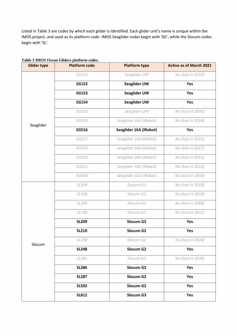
Listed in Table 3 are codes by which each glider is identified. Each glider unit’s name is unique within the
IMOS project, and used as its platform code. IMOS Seaglider codes begin with ‘SG’, while the Slocum codes
begin with ‘SL’.
Table 3 IMOS Ocean Gliders platform codes.
Glider type Platform code Platform type Active as of March 2021
Seaglider
SG151 Seaglider UW No (lost in 2010)
SG152 Seaglider UW Yes
SG153 Seaglider UW Yes
SG154 Seaglider UW Yes
SG155 Seaglider UW No (lost in 2016)
SG514 Seaglider 1kA (iRobot) No (lost in 2014)
SG516 Seaglider 1kA (iRobot) Yes
SG517 Seaglider 1kA (iRobot) No (lost in 2011)
SG519 Seaglider 1kA (iRobot) No (lost in 2011)
SG520 Seaglider 1kA (iRobot) No (lost in 2011)
SG521 Seaglider 1kA (iRobot) No (lost in 2012)
SG540 Seaglider 1kA (iRobot) No (lost in 2018)
Slocum
SL104 Slocum G1 No (lost in 2010)
SL106 Slocum G1 No (lost in 2010)
SL109 Slocum G1 No (lost in 2009)
SL130 Slocum G1 No (lost in 2011)
SL209 Slocum G2 Yes
SL210 Slocum G2 Yes
SL239 Slocum G2 No (lost in 2018)
SL248 Slocum G2 Yes
SL281 Slocum G2 No (lost in 2020)
SL286 Slocum G2 Yes
SL287 Slocum G2 Yes
SL502 Slocum G2 Yes
SL812 Slocum G3 Yes
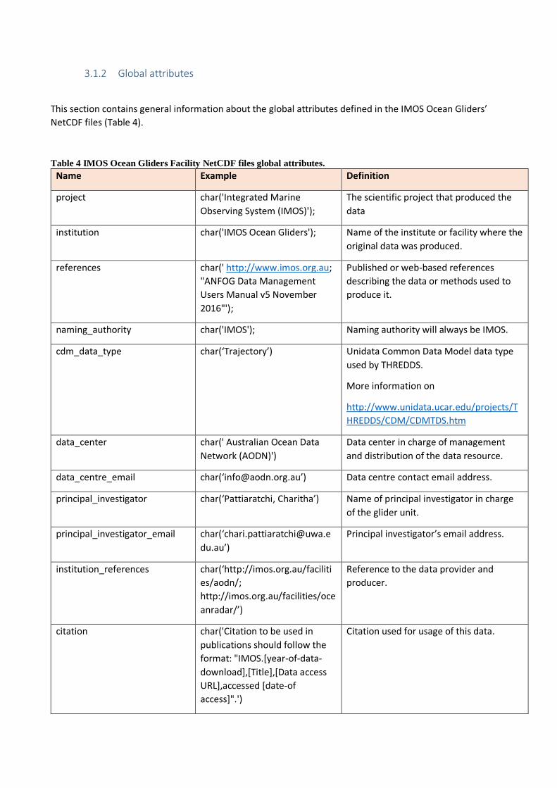
3.1.2 Global attributes
This section contains general information about the global attributes defined in the IMOS Ocean Gliders’
NetCDF files (Table 4).
Table 4 IMOS Ocean Gliders Facility NetCDF files global attributes.
Name Example Definition
project char('Integrated Marine
Observing System (IMOS)');
The scientific project that produced the
data
institution char('IMOS Ocean Gliders'); Name of the institute or facility where the
original data was produced.
references
char(' http://www.imos.org.au;
"ANFOG Data Management
Users Manual v5 November
2016"');
Published or web-based references
describing the data or methods used to
produce it.
naming_authority char('IMOS'); Naming authority will always be IMOS.
cdm_data_type char(‘Trajectory’) Unidata Common Data Model data type
used by THREDDS.
More information on
http://www.unidata.ucar.edu/projects/T
HREDDS/CDM/CDMTDS.htm
data_center char(' Australian Ocean Data
Network (AODN)')
Data center in charge of management
and distribution of the data resource.
data_centre_email char(‘[email protected]’) Data centre contact email address.
principal_investigator char(‘Pattiaratchi, Charitha’) Name of principal investigator in charge
of the glider unit.
principal_investigator_email char(‘[email protected]
du.au’)
Principal investigator’s email address.
institution_references
char(‘http://imos.org.au/faciliti
es/aodn/;
http://imos.org.au/facilities/oce
anradar/’)
Reference to the data provider and
producer.
citation char('Citation to be used in
publications should follow the
format: "IMOS.[year-of-data-
download],[Title],[Data access
URL],accessed [date-of
access]".')
Citation used for usage of this data.
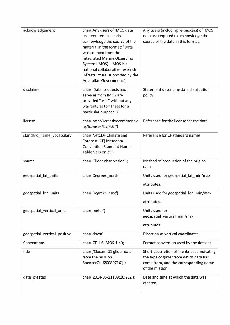
acknowledgement
char(‘Any users of IMOS data
are required to clearly
acknowledge the source of the
material in the format: "Data
was sourced from the
Integrated Marine Observing
System (IMOS) - IMOS is a
national collaborative research
infrastructure, supported by the
Australian Government.’)
Any users (including re-packers) of IMOS
data are required to acknowledge the
source of the data in this format.
disclaimer
char(' Data, products and
services from IMOS are
provided "as is" without any
warranty as to fitness for a
particular purpose.')
Statement describing data distribution
policy.
license char('http://creativecommons.o
rg/licenses/by/4.0/')
Reference for the license for the data
standard_name_vocabulary char('NetCDF Climate and
Forecast (CF) Metadata
Convention Standard Name
Table Version 29')
Reference for CF standard names
source char('Glider observation'); Method of production of the original
data.
geospatial_lat_units char('Degrees_north') Units used for geospatial_lat_min/max
attributes.
geospatial_lon_units char('Degrees_east') Units used for geospatial_lon_min/max
attributes.
geospatial_vertical_units char('meter') Units used for
geospatial_vertical_min/max
attributes.
geospatial_vertical_positive char('down') Direction of vertical coordinates
Conventions char(‘CF-1.6,IMOS-1.4’); Format convention used by the dataset
title char([‘Slocum G1 glider data
from the mission
SpencerGulf20080716’]);
Short description of the dataset indicating
the type of glider from which data has
come from, and the corresponding name
of the mission.
date_created char(‘2014-06-11T09:16:22Z’);
Date and time at which the data was
created.
Format: yyyy-mm-ddTHH:MM:SSZ'
Example: 2008-12-10T09:35:36Z :
December 10th 2008 9:35:36AM
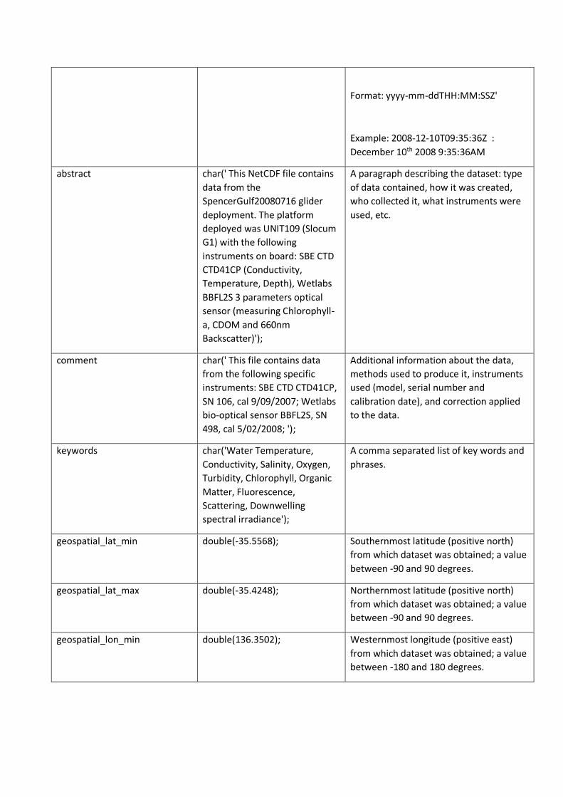
abstract
char(' This NetCDF file contains
data from the
SpencerGulf20080716 glider
deployment. The platform
deployed was UNIT109 (Slocum
G1) with the following
instruments on board: SBE CTD
CTD41CP (Conductivity,
Temperature, Depth), Wetlabs
BBFL2S 3 parameters optical
sensor (measuring Chlorophyll-
a, CDOM and 660nm
Backscatter)');
A paragraph describing the dataset: type
of data contained, how it was created,
who collected it, what instruments were
used, etc.
comment
char(' This file contains data
from the following specific
instruments: SBE CTD CTD41CP,
SN 106, cal 9/09/2007; Wetlabs
bio-optical sensor BBFL2S, SN
498, cal 5/02/2008; ');
Additional information about the data,
methods used to produce it, instruments
used (model, serial number and
calibration date), and correction applied
to the data.
keywords
char('Water Temperature,
Conductivity, Salinity, Oxygen,
Turbidity, Chlorophyll, Organic
Matter, Fluorescence,
Scattering, Downwelling
spectral irradiance');
A comma separated list of key words and
phrases.
geospatial_lat_min
double(-35.5568); Southernmost latitude (positive north)
from which dataset was obtained; a value
between -90 and 90 degrees.
geospatial_lat_max
double(-35.4248); Northernmost latitude (positive north)
from which dataset was obtained; a value
between -90 and 90 degrees.
geospatial_lon_min
double(136.3502);
Westernmost longitude (positive east)
from which dataset was obtained; a value
between -180 and 180 degrees.
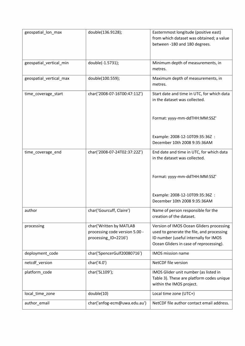
geospatial_lon_max
double(136.9128); Easternmost longitude (positive east)
from which dataset was obtained; a value
between -180 and 180 degrees.
geospatial_vertical_min double(-1.5731); Minimum depth of measurements, in
metres.
geospatial_vertical_max double(100.559); Maximum depth of measurements, in
metres.
time_coverage_start
char(‘2008-07-16T00:47:11Z’) Start date and time in UTC, for which data
in the dataset was collected.
Format: yyyy-mm-ddTHH:MM:SSZ'
Example: 2008-12-10T09:35:36Z :
December 10th 2008 9:35:36AM
time_coverage_end
char(‘2008-07-24T02:37:22Z’) End date and time in UTC, for which data
in the dataset was collected.
Format: yyyy-mm-ddTHH:MM:SSZ'
Example: 2008-12-10T09:35:36Z :
December 10th 2008 9:35:36AM
author char(‘Gourcuff, Claire’) Name of person responsible for the
creation of the dataset.
processing char('Written by MATLAB
processing code version 5.00 -
processing_ID=2216')
Version of IMOS Ocean Gliders processing
used to generate the file, and processing
ID number (useful internally for IMOS
Ocean Gliders in case of reprocessing).
deployment_code char(‘SpencerGulf20080716’) IMOS mission name
netcdf_version char('4.0') NetCDF file version
platform_code char(‘SL109’); IMOS Glider unit number (as listed in
Table 3). These are platform codes unique
within the IMOS project.
local_time_zone double(10) Local time zone (UTC+)
author_email char('[email protected]') NetCDF file author contact email address.

data_mode Char('Delayed Mode') Mode of data processing
history Char(‘2018-11-29T06:11:55Z
Created. 2019-02-18T10:02:17Z
Corrected CTD serial number
and calibration date’)
Audit trail for modifications to the
original data. If no changes have been
made, this contains creation date.
3.1.3 Metadata containers
In each NetCDF datafile, information describing the platform and sensors used, and the deployment itself is
stored in the attributes of empty and dimensionless variables known as ‘containers’. PLATFORM,
DEPLOYMENT and SENSOR are such empty, dimensionless variables. Their associated attributes are as listed
in Table 5.
Table 5 Metadata containers and their attributes. Note: If an attribute value is empty (information unknown), the
attribute does not exist in the NetCDF file.
Variable Attributes Example
PLATFORM
trans_system_id 'Irridium'
positioning_system 'GPS'
platform_type 'Slocum G2'
long_name 'Platform information'
platform_maker 'Teledyne Webb Research'
firmware_version_navigation 7.16
firmware_version_science 7.16
glider_serial_no '209'
battery_type 'Alkaline'
glider_owner 'IMOS Ocean Gliders'
operating_institution 'IMOS Ocean Gliders'
wmo 6801513
DEPLOYMENT
deployment_start_date '2016-03-30-T24:23:29Z'
deployment_start_latitude -29.467 (decimal degrees)
deployment_start_longitude 121.8523 (decimal degrees)
long_name 'Deployment information'
deployment_start_technician 'Thomson, Paul'
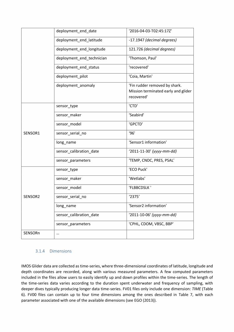
deployment_end_date '2016-04-03-T02:45:17Z'
deployment_end_latitude -17.1947 (decimal degrees)
deployment_end_longitude 121.726 (decimal degrees)
deployment_end_technician 'Thomson, Paul'
deployment_end_status 'recovered'
deployment_pilot 'Coia, Martin'
deployment_anomaly 'Fin rudder removed by shark.
Mission terminated early and glider
recovered'
SENSOR1
sensor_type 'CTD'
sensor_maker 'Seabird'
sensor_model 'GPCTD'
sensor_serial_no '96'
long_name 'Sensor1 information'
sensor_calibration_date ‘2011-11-30’ (yyyy-mm-dd)
sensor_parameters 'TEMP, CNDC, PRES, PSAL'
SENSOR2
sensor_type 'ECO Puck'
sensor_maker 'Wetlabs'
sensor_model 'FLBBCDSLK '
sensor_serial_no ‘2375’
long_name 'Sensor2 information'
sensor_calibration_date '2011-10-06' (yyyy-mm-dd)
sensor_parameters 'CPHL, CDOM, VBSC, BBP'
SENSORn …
3.1.4 Dimensions
IMOS Glider data are collected as time-series, where three-dimensional coordinates of latitude, longitude and
depth coordinates are recorded, along with various measured parameters. A few computed parameters
included in the files allow users to easily identify up and down profiles within the time-series. The length of
the time-series data varies according to the duration spent underwater and frequency of sampling, with
deeper dives typically producing longer data time-series. FV01 files only include one dimension: TIME (Table
6). FV00 files can contain up to four time dimensions among the ones described in Table 7, with each
parameter associated with one of the available dimensions (see EGO (2013)).
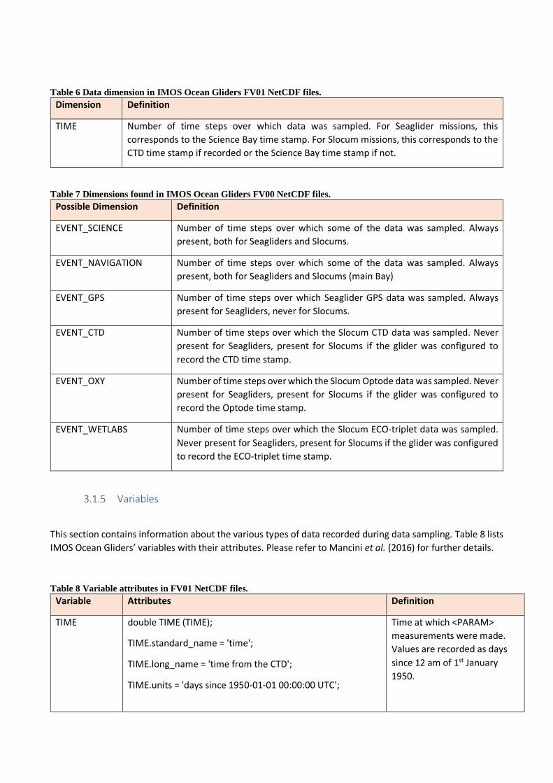
Table 6 Data dimension in IMOS Ocean Gliders FV01 NetCDF files.
Dimension Definition
TIME Number of time steps over which data was sampled. For Seaglider missions, this
corresponds to the Science Bay time stamp. For Slocum missions, this corresponds to the
CTD time stamp if recorded or the Science Bay time stamp if not.
Table 7 Dimensions found in IMOS Ocean Gliders FV00 NetCDF files.
Possible Dimension Definition
EVENT_SCIENCE Number of time steps over which some of the data was sampled. Always
present, both for Seagliders and Slocums.
EVENT_NAVIGATION Number of time steps over which some of the data was sampled. Always
present, both for Seagliders and Slocums (main Bay)
EVENT_GPS Number of time steps over which Seaglider GPS data was sampled. Always
present for Seagliders, never for Slocums.
EVENT_CTD Number of time steps over which the Slocum CTD data was sampled. Never
present for Seagliders, present for Slocums if the glider was configured to
record the CTD time stamp.
EVENT_OXY Number of time steps over which the Slocum Optode data was sampled. Never
present for Seagliders, present for Slocums if the glider was configured to
record the Optode time stamp.
EVENT_WETLABS Number of time steps over which the Slocum ECO-triplet data was sampled.
Never present for Seagliders, present for Slocums if the glider was configured
to record the ECO-triplet time stamp.
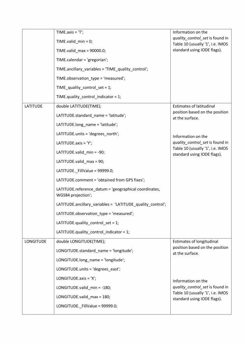
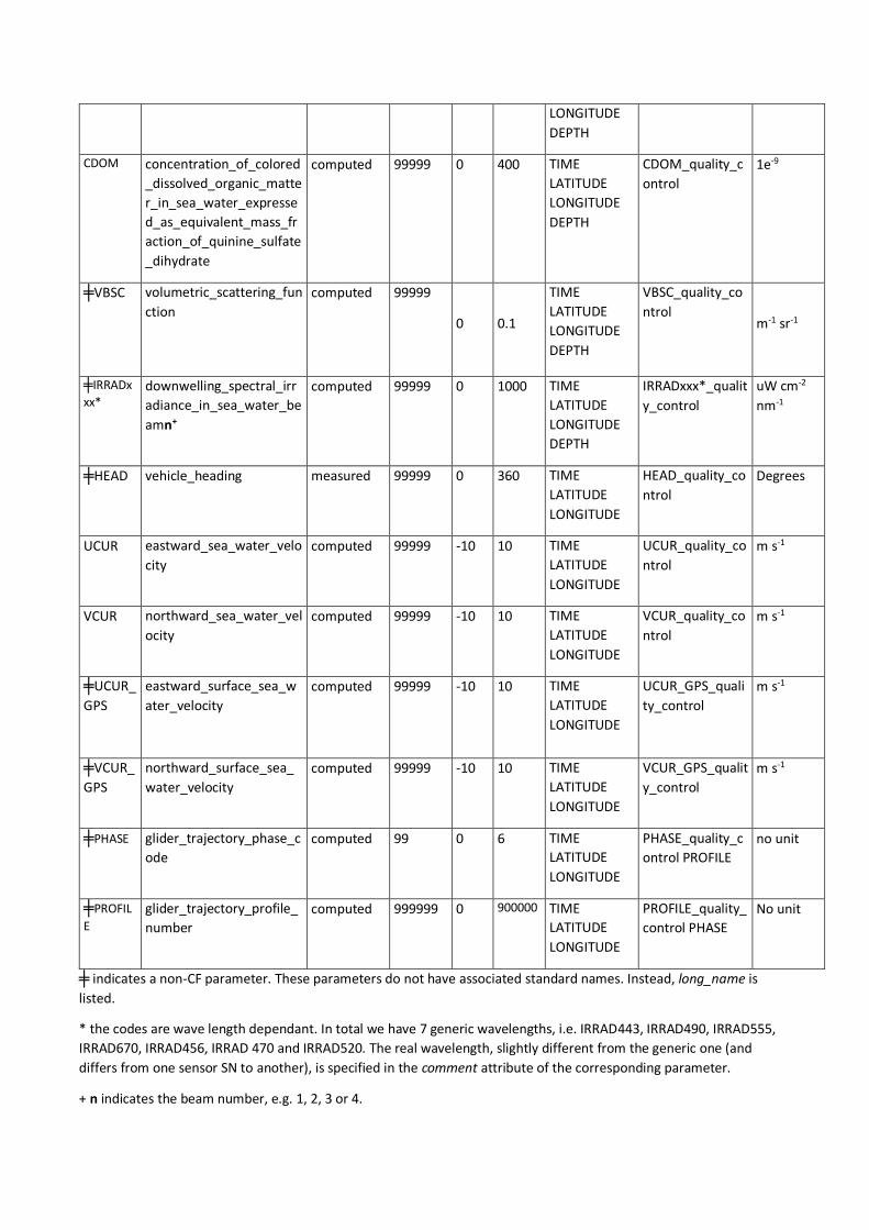
3.1.5 Variables
This section contains information about the various types of data recorded during data sampling. Table 8 lists
IMOS Ocean Gliders’ variables with their attributes. Please refer to Mancini et al. (2016) for further details.
Table 8 Variable attributes in FV01 NetCDF files.
Variable Attributes Definition
TIME double TIME (TIME);
TIME.standard_name = 'time';
TIME.long_name = 'time from the CTD';
TIME.units = 'days since 1950-01-01 00:00:00 UTC';
Time at which <PARAM>
measurements were made.
Values are recorded as days
since 12 am of 1st January
1950.
TIME.axis = 'T';
TIME.valid_min = 0;
TIME.valid_max = 90000.0;
TIME.calendar = 'gregorian';
TIME.ancillary_variables = 'TIME_quality_control';
TIME.observation_type = ‘measured’;
TIME_quality_control_set = 1;
TIME.quality_control_indicator = 1;
Information on the
quality_control_set is found in
Table 10 (usually ‘1’, i.e. IMOS
standard using IODE flags).
LATITUDE double LATITUDE(TIME);
LATITUDE.standard_name = 'latitude';
LATITUDE.long_name = 'latitude';
LATITUDE.units = 'degrees_north';
LATITUDE.axis = 'Y';
LATITUDE.valid_min = -90;
LATITUDE.valid_max = 90;
LATITUDE._FillValue = 99999.0;
LATITUDE.comment = ‘obtained from GPS fixes’;
LATITUDE.reference_datum = 'geographical coordinates,
WGS84 projection';
LATITUDE.ancillary_variables = 'LATITUDE_quality_control';
LATITUDE.observation_type = ‘measured’;
LATITUDE.quality_control_set = 1;
LATITUDE.quality_control_indicator = 1;
Estimates of latitudinal
position based on the position
at the surface.
Information on the
quality_control_set is found in
Table 10 (usually ‘1’, i.e. IMOS
standard using IODE flags).
LONGITUDE double LONGITUDE(TIME);
LONGITUDE.standard_name = ‘longitude';
LONGITUDE.long_name = 'longitude';
LONGITUDE.units = 'degrees_east';
LONGITUDE.axis = 'X';
LONGITUDE.valid_min = -180;
LONGITUDE.valid_max = 180;
LONGITUDE._FillValue = 99999.0;
Estimates of longitudinal
position based on the position
at the surface.
Information on the
quality_control_set is found in
Table 10 (usually ‘1’, i.e. IMOS
standard using IODE flags).
LONGITUDE.comment = 'obtained from GPS fixes';
LONGITUDE.reference_datum = 'geographical coordinates,
WGS84 projection';
LONGITUDE.ancillary_variables =
'LATITUDE_quality_control';
LONGITUDE.observation_type = ‘measured’;
LONGITUDE.quality_control_set = 1;
LONGITUDE.quality_control_indicator = 1;
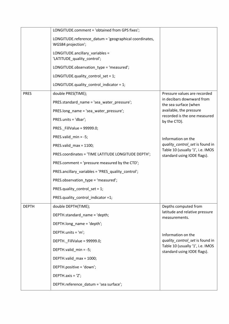
PRES double PRES(TIME);
PRES.standard_name = 'sea_water_pressure';
PRES.long_name = 'sea_water_pressure';
PRES.units = 'dbar';
PRES._FillValue = 99999.0;
PRES.valid_min = -5;
PRES.valid_max = 1100;
PRES.coordinates = 'TIME LATITUDE LONGITUDE DEPTH';
PRES.comment = 'pressure measured by the CTD';
PRES.ancillary_variables = 'PRES_quality_control';
PRES.observation_type = ‘measured’;
PRES.quality_control_set = 1;
PRES.quality_control_indicator =1;
Pressure values are recorded
in decibars downward from
the sea surface (when
available, the pressure
recorded is the one measured
by the CTD).
Information on the
quality_control_set is found in
Table 10 (usually ‘1’, i.e. IMOS
standard using IODE flags).
DEPTH double DEPTH(TIME);
DEPTH.standard_name = 'depth;
DEPTH.long_name = 'depth';
DEPTH.units = 'm';
DEPTH._FillValue = 99999.0;
DEPTH.valid_min = -5;
DEPTH.valid_max = 1000;
DEPTH.positive = ‘down’;
DEPTH.axis = ‘Z’;
DEPTH.reference_datum = 'sea surface’;
Depths computed from
latitude and relative pressure
measurements.
Information on the
quality_control_set is found in
Table 10 (usually ‘1’, i.e. IMOS
standard using IODE flags).
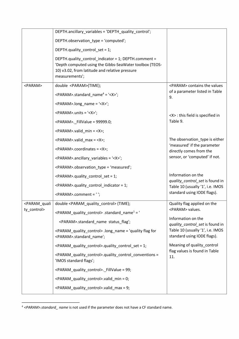
DEPTH.ancillary_variables = 'DEPTH_quality_control';
DEPTH.observation_type = ‘computed’;
DEPTH.quality_control_set = 1;
DEPTH.quality_control_indicator = 1; DEPTH.comment =
'Depth computed using the Gibbs-SeaWater toolbox (TEOS-
10) v3.02, from latitude and relative pressure
measurements';
<PARAM> double <PARAM>(TIME);
<PARAM>.standard_name4 = '<X>’;
<PARAM>.long_name = ‘<X>’;
<PARAM>.units = '<X>';
<PARAM>._FillValue = 99999.0;
<PARAM>.valid_min = <X>;
<PARAM>.valid_max = <X>;
<PARAM>.coordinates = <X>;
<PARAM>.ancillary_variables = ‘<X>’;
<PARAM>.observation_type = ‘measured’;
<PARAM>.quality_control_set = 1;
<PARAM>.quality_control_indicator = 1;
<PARAM>.comment = ‘ ‘;
<PARAM> contains the values
of a parameter listed in Table
9.
<X> : this field is specified in
Table 9.
The observation_type is either
‘measured’ if the parameter
directly comes from the
sensor, or ‘computed’ if not.
Information on the
quality_control_set is found in
Table 10 (usually ‘1’, i.e. IMOS
standard using IODE flags).
<PARAM_quali
ty_control>
double <PARAM_quality_control> (TIME);
<PARAM_quality_control> .standard_name1 = '
<PARAM>.standard_name status_flag';
<PARAM_quality_control> .long_name = 'quality flag for
<PARAM>.standard_name';
<PARAM_quality_control>.quality_control_set = 1;
<PARAM_quality_control>.quality_control_conventions =
'IMOS standard flags';
<PARAM_quality_control>._FillValue = 99;
<PARAM_quality_control>.valid_min = 0;
<PARAM_quality_control>.valid_max = 9;
Quality flag applied on the
<PARAM> values.
Information on the
quality_control_set is found in
Table 10 (usually ‘1’, i.e. IMOS
standard using IODE flags).
Meaning of quality_control
flag values is found in Table
11.
4 <PARAM>.standard_ name is not used if the parameter does not have a CF standard name.
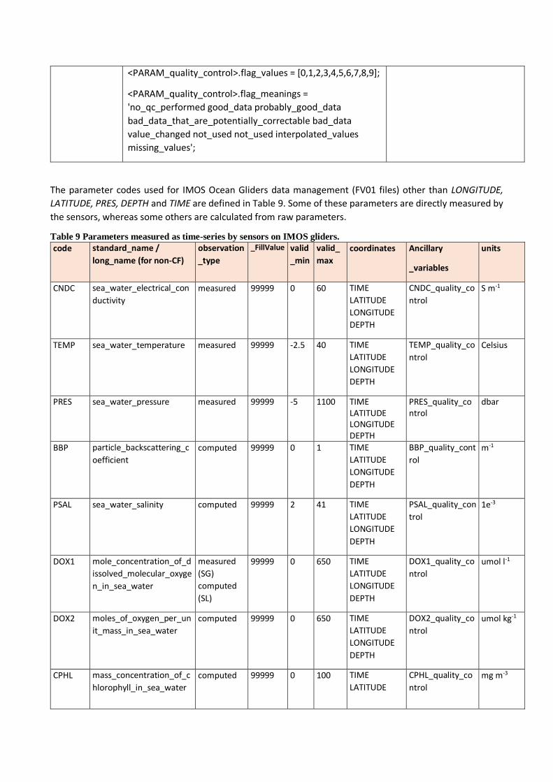
<PARAM_quality_control>.flag_values = [0,1,2,3,4,5,6,7,8,9];
<PARAM_quality_control>.flag_meanings =
'no_qc_performed good_data probably_good_data
bad_data_that_are_potentially_correctable bad_data
value_changed not_used not_used interpolated_values
missing_values';
The parameter codes used for IMOS Ocean Gliders data management (FV01 files) other than LONGITUDE,
LATITUDE, PRES, DEPTH and TIME are defined in Table 9. Some of these parameters are directly measured by
the sensors, whereas some others are calculated from raw parameters.
Table 9 Parameters measured as time-series by sensors on IMOS gliders.
code standard_name /
long_name (for non-CF)
observation
_type
_FillValue valid
_min
valid_
max
coordinates Ancillary
_variables
units
CNDC
sea_water_electrical_con
ductivity
measured 99999 0 60 TIME
LATITUDE
LONGITUDE
DEPTH
CNDC_quality_co
ntrol
S m-1
TEMP
sea_water_temperature measured 99999 -2.5 40 TIME
LATITUDE
LONGITUDE
DEPTH
TEMP_quality_co
ntrol
Celsius
PRES sea_water_pressure measured 99999 -5 1100 TIME LATITUDE LONGITUDE DEPTH
PRES_quality_control
dbar
BBP particle_backscattering_c
oefficient
computed 99999 0 1 TIME
LATITUDE
LONGITUDE
DEPTH
BBP_quality_cont
rol
m-1
PSAL
sea_water_salinity computed 99999 2 41 TIME
LATITUDE
LONGITUDE
DEPTH
PSAL_quality_con
trol
1e-3
DOX1 mole_concentration_of_d
issolved_molecular_oxyge
n_in_sea_water
measured
(SG)
computed
(SL)
99999 0 650 TIME
LATITUDE
LONGITUDE
DEPTH
DOX1_quality_co
ntrol
umol l-1
DOX2 moles_of_oxygen_per_un
it_mass_in_sea_water
computed 99999 0 650 TIME
LATITUDE
LONGITUDE
DEPTH
DOX2_quality_co
ntrol
umol kg-1
CPHL
mass_concentration_of_c
hlorophyll_in_sea_water
computed 99999 0 100 TIME
LATITUDE
CPHL_quality_co
ntrol
mg m-3
LONGITUDE
DEPTH
CDOM
concentration_of_colored
_dissolved_organic_matte
r_in_sea_water_expresse
d_as_equivalent_mass_fr
action_of_quinine_sulfate
_dihydrate
computed 99999 0 400 TIME
LATITUDE
LONGITUDE
DEPTH
CDOM_quality_c
ontrol
1e-9
╪VBSC volumetric_scattering_fun
ction
computed 99999
0
0.1
TIME
LATITUDE
LONGITUDE
DEPTH
VBSC_quality_co
ntrol
m-1 sr-1
╪IRRADx
xx*
downwelling_spectral_irr
adiance_in_sea_water_be
amn+
computed 99999 0 1000 TIME
LATITUDE
LONGITUDE
DEPTH
IRRADxxx*_qualit
y_control
uW cm-2
nm-1
╪HEAD vehicle_heading measured 99999 0 360 TIME
LATITUDE
LONGITUDE
HEAD_quality_co
ntrol
Degrees
UCUR
eastward_sea_water_velo
city
computed 99999 -10 10 TIME
LATITUDE
LONGITUDE
UCUR_quality_co
ntrol
m s-1
VCUR
northward_sea_water_vel
ocity
computed 99999 -10 10 TIME
LATITUDE
LONGITUDE
VCUR_quality_co
ntrol
m s-1
╪UCUR_
GPS
eastward_surface_sea_w
ater_velocity
computed 99999 -10 10 TIME
LATITUDE
LONGITUDE
UCUR_GPS_quali
ty_control
m s-1
╪VCUR_
GPS
northward_surface_sea_
water_velocity
computed 99999 -10 10 TIME
LATITUDE
LONGITUDE
VCUR_GPS_qualit
y_control
m s-1
╪PHASE
glider_trajectory_phase_c
ode
computed 99 0 6 TIME
LATITUDE
LONGITUDE
PHASE_quality_c
ontrol PROFILE
no unit
╪PROFIL
E
glider_trajectory_profile_
number
computed 999999 0 900000 TIME
LATITUDE
LONGITUDE
PROFILE_quality_
control PHASE
No unit
╪ indicates a non-CF parameter. These parameters do not have associated standard names. Instead, long_name is
listed.
* the codes are wave length dependant. In total we have 7 generic wavelengths, i.e. IRRAD443, IRRAD490, IRRAD555,
IRRAD670, IRRAD456, IRRAD 470 and IRRAD520. The real wavelength, slightly different from the generic one (and
differs from one sensor SN to another), is specified in the comment attribute of the corresponding parameter.
+ n indicates the beam number, e.g. 1, 2, 3 or 4.
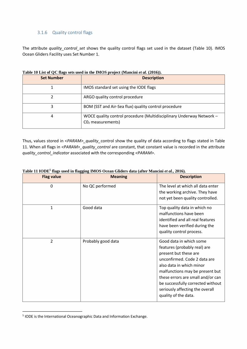
3.1.6 Quality control flags
The attribute quality_control_set shows the quality control flags set used in the dataset (Table 10). IMOS
Ocean Gliders Facility uses Set Number 1.
Table 10 List of QC flags sets used in the IMOS project (Mancini et al. (2016)).
Set Number Description
1 IMOS standard set using the IODE flags
2 ARGO quality control procedure
3 BOM (SST and Air-Sea flux) quality control procedure
4 WOCE quality control procedure (Multidisciplinary Underway Network –
C02 measurements)
Thus, values stored in <PARAM>_quality_control show the quality of data according to flags stated in Table
11. When all flags in <PARAM>_quality_control are constant, that constant value is recorded in the attribute
quality_control_indicator associated with the corresponding <PARAM>.
Table 11 IODE5 flags used in flagging IMOS Ocean Gliders data (after Mancini et al., 2016).
Flag value Meaning Description
0 No QC performed The level at which all data enter
the working archive. They have
not yet been quality controlled.
1 Good data Top quality data in which no
malfunctions have been
identified and all real features
have been verified during the
quality control process.
2 Probably good data Good data in which some
features (probably real) are
present but these are
unconfirmed. Code 2 data are
also data in which minor
malfunctions may be present but
these errors are small and/or can
be successfully corrected without
seriously affecting the overall
quality of the data.
5 IODE is the International Oceanographic Data and Information Exchange.
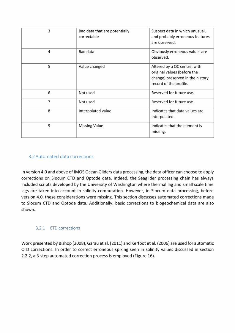
3 Bad data that are potentially
correctable
Suspect data in which unusual,
and probably erroneous features
are observed.
4 Bad data Obviously erroneous values are
observed.
5 Value changed Altered by a QC centre, with
original values (before the
change) preserved in the history
record of the profile.
6 Not used Reserved for future use.
7 Not used Reserved for future use.
8 Interpolated value Indicates that data values are
interpolated.
9 Missing Value Indicates that the element is
missing.
3.2 Automated data corrections
In version 4.0 and above of IMOS Ocean Gliders data processing, the data officer can choose to apply
corrections on Slocum CTD and Optode data. Indeed, the Seaglider processing chain has always
included scripts developed by the University of Washington where thermal lag and small scale time
lags are taken into account in salinity computation. However, in Slocum data processing, before
version 4.0, these considerations were missing. This section discusses automated corrections made
to Slocum CTD and Optode data. Additionally, basic corrections to biogeochemical data are also
shown.
3.2.1 CTD corrections
Work presented by Bishop (2008), Garau et al. (2011) and Kerfoot et al. (2006) are used for automatic
CTD corrections. In order to correct erroneous spiking seen in salinity values discussed in section
2.2.2, a 3-step automated correction process is employed (Figure 16).
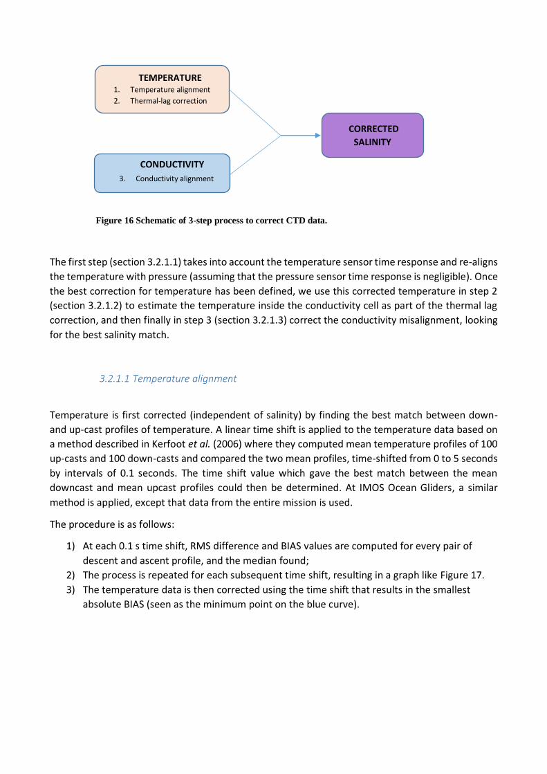
The first step (section 3.2.1.1) takes into account the temperature sensor time response and re-aligns
the temperature with pressure (assuming that the pressure sensor time response is negligible). Once
the best correction for temperature has been defined, we use this corrected temperature in step 2
(section 3.2.1.2) to estimate the temperature inside the conductivity cell as part of the thermal lag
correction, and then finally in step 3 (section 3.2.1.3) correct the conductivity misalignment, looking
for the best salinity match.
3.2.1.1 Temperature alignment
Temperature is first corrected (independent of salinity) by finding the best match between down-
and up-cast profiles of temperature. A linear time shift is applied to the temperature data based on
a method described in Kerfoot et al. (2006) where they computed mean temperature profiles of 100
up-casts and 100 down-casts and compared the two mean profiles, time-shifted from 0 to 5 seconds
by intervals of 0.1 seconds. The time shift value which gave the best match between the mean
downcast and mean upcast profiles could then be determined. At IMOS Ocean Gliders, a similar
method is applied, except that data from the entire mission is used.
The procedure is as follows:
1) At each 0.1 s time shift, RMS difference and BIAS values are computed for every pair of
descent and ascent profile, and the median found;
2) The process is repeated for each subsequent time shift, resulting in a graph like Figure 17.
3) The temperature data is then corrected using the time shift that results in the smallest
absolute BIAS (seen as the minimum point on the blue curve).
TEMPERATURE 1. Temperature alignment
2. Thermal-lag correction
CORRECTED
SALINITY
CONDUCTIVITY
3. Conductivity alignment
Figure 16 Schematic of 3-step process to correct CTD data.
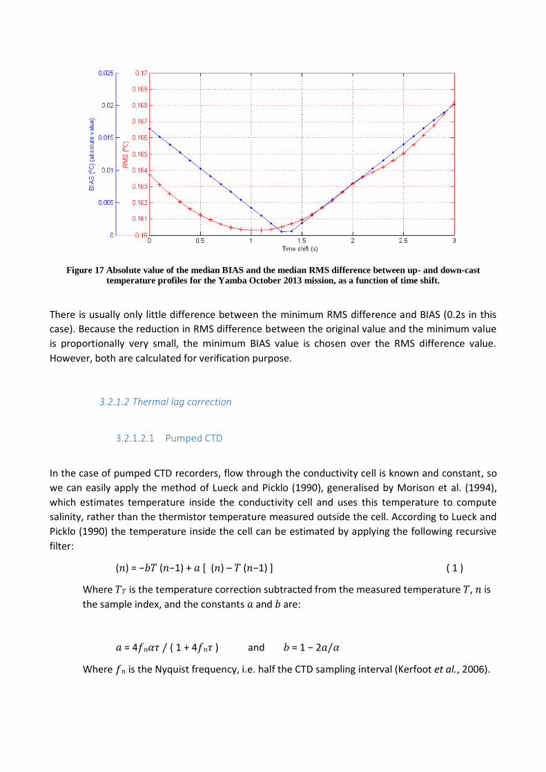
Figure 17 Absolute value of the median BIAS and the median RMS difference between up- and down-cast
temperature profiles for the Yamba October 2013 mission, as a function of time shift.
There is usually only little difference between the minimum RMS difference and BIAS (0.2s in this
case). Because the reduction in RMS difference between the original value and the minimum value
is proportionally very small, the minimum BIAS value is chosen over the RMS difference value.
However, both are calculated for verification purpose.
3.2.1.2 Thermal lag correction
3.2.1.2.1 Pumped CTD
In the case of pumped CTD recorders, flow through the conductivity cell is known and constant, so
we can easily apply the method of Lueck and Picklo (1990), generalised by Morison et al. (1994),
which estimates temperature inside the conductivity cell and uses this temperature to compute
salinity, rather than the thermistor temperature measured outside the cell. According to Lueck and
Picklo (1990) the temperature inside the cell can be estimated by applying the following recursive
filter:
(𝑛) = −𝑏𝑇 (𝑛−1) + 𝑎 [ (𝑛) – 𝑇 (𝑛−1) ] ( 1 )
Where 𝑇𝑇 is the temperature correction subtracted from the measured temperature 𝑇, 𝑛 is
the sample index, and the constants 𝑎 and 𝑏 are:
𝑎 = 4𝑓𝑛𝛼𝜏 / ( 1 + 4𝑓𝑛𝜏 ) and 𝑏 = 1 − 2𝑎/𝛼
Where 𝑓𝑛 is the Nyquist frequency, i.e. half the CTD sampling interval (Kerfoot et al., 2006).
Morison et al. (1994) show that if the flow in the conductivity cell is constant, α and τ can be
estimated using the following empirical relation:
𝛼 = 0.0264 𝑉−1 + 0.0135 and 𝜏 = 2.7858 𝑉−1/2 + 7.1499 ( 2 )
In the case of GPCTD recorders used in IMOS Slocum gliders, the flow rate in the conductivity cell is
10 ml/s, the volume of the cell is 3 ml and its length 146mm, which gives a velocity:
𝑉 = 0.4867 𝑚 𝑠−1
As this velocity falls within the valid range stated by Morison et al. (1994), 𝑎 and 𝑏 can then be
computed and the temperature inside the conductivity cell derived using equations (2) and (1).
3.2.1.2.2 Unpumped CTD
When correcting data from unpumped CTD, 𝛼 and 𝜏 from equation (2) are computed by estimating
that velocity for each profile is the same as the glider velocity of travel through the water column.
Temperature within the conductivity cell is then calculated by applying equations (1) and (2).
This method was chosen over the method proposed by Garau et al. (2011) which had been
formulated as an improvement of the commonly used Morison et al. (1994) method so as to take
into account for variable flow speed inside the conductivity cell, irregular sampling intervals etc., as
an un-pumped glider-mounted CTD would have. However, our testing found that using their method
did not lead to better results than when recomputing α and τ using an estimate of the glider’s velocity
across the water column, V, per profile. Moreover, their method was time consuming, especially
when taking into account the conductivity sensor time response, which forced us to perform many
iterations to get the best parameters and time lag.
3.2.1.3 Conductivity alignment
Conductivity time lag is estimated after the completion of temperature alignment and thermal lag
correction. It was found that conductivity time lag is not constant throughout the whole deployment.
It is speculated that this may be due to geometrically induced time lag, i.e. the conductivity cell is a
distance away from the pressure sensor, and pitch and dive rate of the glider are too variable on a
single profile. Our efforts to correct for geometric time lag failed. The method employed for
conductivity alignment which brought good results is a follows:

1) Determine the time shift in conductivity data that produces the best match (smallest RMS difference) for each individual pair of computed salinity up- and down-cast profile (values tested at increasing 0.1s time shift intervals). The RMS difference is used for this estimate rather than the BIAS value, due to the presence of spikes in salinity profiles which can change the sign of the BIAS difference between the 2 profiles of a dive-climb pair.
Figure 18 Salinity RMS difference between consecutive up- and down-cast pair is greatly reduced by the
introduction of a best time shift in conductivity data for each individual pair.
In the Yamba20120904 mission for instance, applying the best time shift for each individual dive-climb pair in conductivity data, successfully decreases the salinity RMS difference significantly from values of the order of 0.1 psu (blue dots) to the order of 0.01 psu (red dots) (Figure 18).
2) When a best time shift for conductivity has been determined for each and every individual
dive-climb pair, their median is found (Figure 19) and applied to the entire conductivity time-series dataset to correct its alignment.
Figure 19 Conductivity time delay (in seconds) by pair of profiles, from beginning of the Yamba20120904 mission
(left) to the end mission (right). The red line is the median time shift (0.9s here).
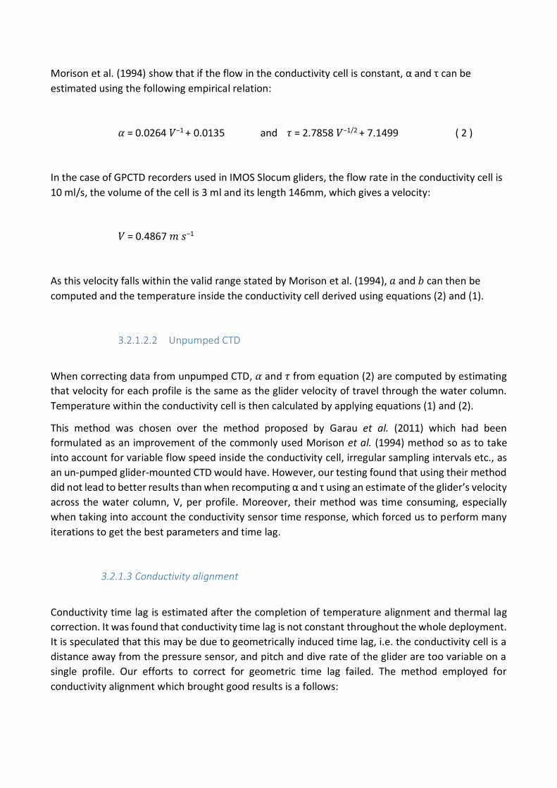
The effect of the abovementioned CTD corrections can be seen in Figure 20 where time lag corrections and thermal lag correction are applied separately to data from the Kimberley20120914 mission CTD data.
Figure 20 (Left) Uncorrected raw salinity data from 4 profile pairs, (middle) only temperature and conductivity
alignments corrected, (right) thermal lag corrected as well as temperature and conductivity alignment.
Comparing the three plots in Figure 20, it can be seen that the erroneous spikes seen in raw data (left plot) are significantly reduced by corrections in temperature and conductivity alignment (middle plot). And this is improved further with the addition of thermal lag correction (right plot).
As a result of these corrections, much of the salinity spiking problems described in section 2.2.2 can
be largely minimised (see Figure 21).
Figure 21 Salinity profile no. 4114 from the Yamba20120904 mission: (blue) raw salinity, (red) corrected salinity.

3.2.2 Oxygen Optode corrections
To improve dissolved oxygen data (MOLAR_DOXY, as internally computed by the glider), re-
computed must be performed using corrected Optode BPHASE measurements, corrected CTD
temperature data and Optode calibration coefficients provided by Aanderaa for each sensor6.
The CTD temperature has now been corrected for short term mismatch with the CTD pressure (see section 3.2.1.1), so BPHASE data must also be aligned with pressure. Moreover, because the Optode is separated from the pressure sensor by a distance of 90cm on the Slocum glider (Figure 22), at typically slow speed of glider travel, this distance induces a non-negligible time difference between when the pressure and the BPHASE measurements are recorded, which needs to be accounted for (3.2.2.1). Subsequently, the lag resulting from BPHASE sensor response time must also be minimised (3.2.2.2). Finally, we combine this corrected BPHASE data with the CTD temperature and the calibration coefficients, to get the final corrected dissolved oxygen data, in μmol/L.
3.2.2.1 Geometrical alignment
On Slocum gliders, the Optode is installed aft, close to the fin, and the CTD is installed toward the
middle of the glider, close to the wings (Figure 22).
Figure 22 Schematic diagram of Slocum glider (After AUVAC, 2018).
6 For this re-computation to be possible, both the temperature and BPHASE data must share the same time axis, thus linearly time-interpolated CTD temperature is used.

The time, 𝜏, taken to travel the 90cm distance between the Optode and CTD recorder is:
𝜏 = 𝑑
𝑣
where d is the distance between the sensors and v is the glider velocity of travel, i.e.
𝑣 = 𝑟
sin 𝜃
where r is dive rate (m/s) and 𝜃 is glider pitch.
Figure 23 Glider orientation during descent. (p: pressure, t: temperature, o: oxygen)
Thus, the time delay between oxygen (or BPHASE) and pressure is:
𝜏 = 𝑑. 𝑠𝑖𝑛𝜃
𝑟
Applying the measured distance between the sensors d = 0.9m, and ideal values for glider travel, r =
0.1 m/s, 𝜃=26°,
𝜏 = 3.9450 s
However, in practice, the glider travels with varying pitch and dive rate. Depending on the ballast,
the average pitch (in absolute value) on dives can significantly depart from the average pitch on
climbs, so the time delay, 𝜏, also varies between dive and climb. Therefore, in order to account for
this, 𝜏 is found for each cast using the average pitch and dive rate on that particular cast. Then, the
results for the whole mission are filtered to avoid extreme values (e.g. see Figure 24). Finally, using
the filtered values of 𝜏, a linear time shift is applied to the BPHASE data to correct for geometrical
alignment.
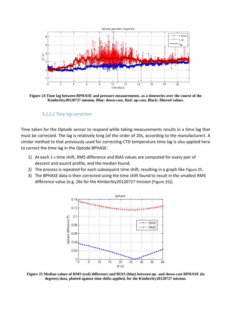
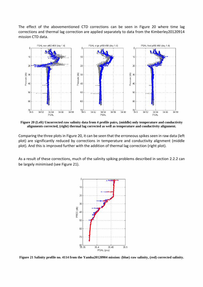
Figure 24 Time lag between BPHASE and pressure measurements, as a timeseries over the course of the
Kimberley20120727 mission. Blue: down-cast, Red: up-cast, Black: filtered values.
3.2.2.2 Time lag correction
Time taken for the Optode sensor to respond while taking measurements results in a time lag that
must be corrected. The lag is relatively long (of the order of 20s, according to the manufacturer). A
similar method to that previously used for correcting CTD temperature time lag is also applied here
to correct the time lag in the Optode BPHASE:
1) At each 1 s time shift, RMS difference and BIAS values are computed for every pair of
descent and ascent profile, and the median found;
2) The process is repeated for each subsequent time shift, resulting in a graph like Figure 25.
3) The BPHASE data is then corrected using the time shift found to result in the smallest RMS
difference value (e.g. 26s for the Kimberley20120727 mission (Figure 25)).
Figure 25 Median values of RMS (red) difference and BIAS (blue) between up- and down-cast BPHASE (in
degrees) data, plotted against time shifts applied, for the Kimberley20120727 mission.

For data from the Kimberley20120727 mission, a linear time shift of 26s minimised the dissymmetry
previously seen in the raw BPHASE data (Figure 26).
Figure 26 (Top) Uncorrected BPHASE data exhibiting dissymmetry between up- and down-casts; (bottom)
symmetry between up- and down-casts is improved by 26s time lag correction.
With BPHASE corrected for geometrical lag and sensor time lag, the concentration of dissolved oxygen is finally re-computed as described in section 2.2.3, using manufacturer calibration coefficients, temperature data from the CTD instead of from the Optode (time interpolated to match with the Optode BPHASE), and with compensation for salinity effects also applied.
From Figure 27, it can be seen that the uncorrected dissolved oxygen data directly reported by the Optode (top plot) is significantly improved by corrections to BPHASE to account for geometrical and sensor lags (middle plot). Data on dive and climb profiles become much more symmetrical. Substituting Optode temperature data with CTD temperature in calculations further improves the quality of the oxygen data (bottom plot).
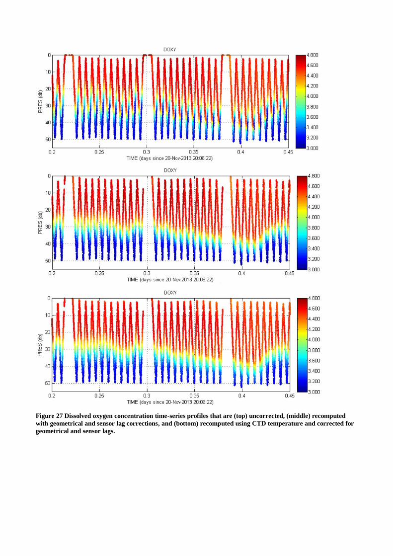
Figure 27 Dissolved oxygen concentration time-series profiles that are (top) uncorrected, (middle) recomputed
with geometrical and sensor lag corrections, and (bottom) recomputed using CTD temperature and corrected for
geometrical and sensor lags.
In future, our Optode data corrections will include the application of pressure compensation also (as recommended by the manufacturer).
This will involve multiplying the oxygen concentration by a factor F:
𝐹 = 1 +0.032 × 𝑝𝑟𝑒𝑠𝑠𝑢𝑟𝑒
1000
where pressure is measured in dbar.
The pressure effect is small in shallow water (F=1.0064 for 200db), but becomes more significant for
deep Slocum missions where the glider reaches pressures of up to 1000db.
3.2.3 Bio-optical data corrections
No automatic corrections to bio-optical data are applied if less than 1% are negative values.
Otherwise, the factory calibrated dark count value is corrected. This is performed to Chlorophyll-a,
CDOM fluorescence and downwelling spectral irradiance data by iteratively decreasing the dark
counts until less than 1% of computed values are negative. Subsequently, the corrected data are
recomputed using the new dark count according to the method described in section 2.2.5.
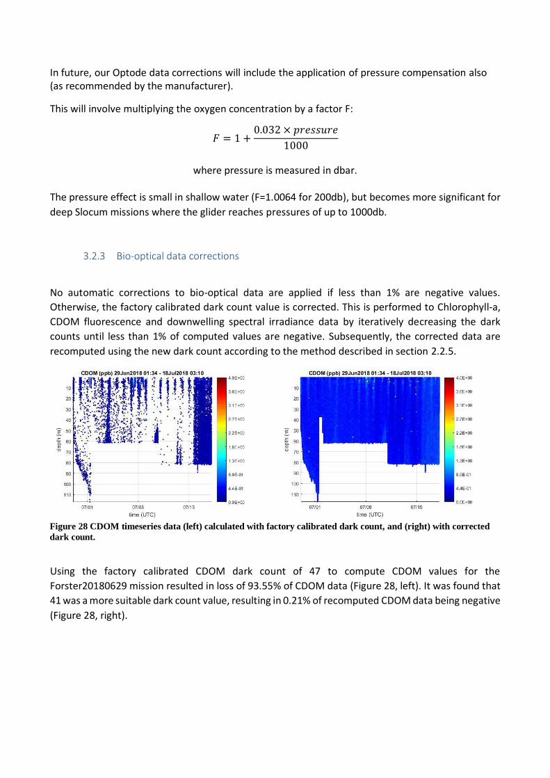
Using the factory calibrated CDOM dark count of 47 to compute CDOM values for the
Forster20180629 mission resulted in loss of 93.55% of CDOM data (Figure 28, left). It was found that
41 was a more suitable dark count value, resulting in 0.21% of recomputed CDOM data being negative
(Figure 28, right).
Figure 28 CDOM timeseries data (left) calculated with factory calibrated dark count, and (right) with corrected
dark count.
4 Automatic Quality Tests
This section describes a series of QC tests that are automatically run to flag scientific data.
It should be noted because GPS location fixes of the glider can be obtained only when the glider has
surfaced, where the glider is travelling underwater, LONGITUDE and LATITUDE values are linearly
interpolated between the 2 GPS fixes obtained at the ocean surface at either end of the submerged
segment. Thus, LONGITUDE_quality_control and LATITUDE_quality_control are flagged with 8 accordingly
(see Table 11). On the other hand, if some of the science data have been slightly interpolated to match
with the single time dimension found in FV01 files, they are not flagged to 8.
4.1 Impossible date test
The impossible date test checks that time values are within the timeframe associated with the
deployment (defined in the deployment_start_date and deployment_end_date attributes of the
variable DEPLOYMENT). All data outside of this timeframe are removed from the dataset.
4.2 Impossible location test
The impossible location test requires that the latitude and longitude that position the observations
are sensible. LATITUDE or LONGITUDE data that fail this test are flagged with 4 (Table 11).
Latitude in range -90 to 90 degrees
Longitude in range -180 to 180 degrees
Correspondingly, good scientific data recorded at unknown locations (i.e. flagged as bad or missing)
then receive a flag of QC=3.
4.3 Range test
The range test applies a gross filter on observed values for the measured scientific parameters which
must accommodate all expected extremes encountered in the oceans around Australia. Valid maxima
and minima as listed inTable 9 are tested, except for the engineering parameters HEAD, UCUR and
VCUR for which no QC is performed (QC flag = 0). A QC flag of 4 is applied to data that fail this test.
4.4 Spike test
The spike test is based on Argo Data Management (Argo, 2013) for temperature and salinity. A
difference between sequential measurements, where one measurement is quite different than
adjacent ones, is a spike in both size and gradient. The test does not consider the differences in depth,
but assumes a sampling that adequately reproduces the temperature and salinity changes with
depth. The algorithm is used on both the temperature and salinity profiles.
Test value = | V2 - (V3 + V1)/2 | - | (V3 - V1) / 2 |
where V2 is the measurement being tested as a spike, and V1 and V3 are the values above and
below.
Temperature:
The V2 value is flagged (QC flag = 4) when
the test value exceeds 6.0 degree C. for pressures less than 500 db or
the test value exceeds 2.0 degree C. for pressures greater than or equal to 500 db
Salinity:
The V2 value is flagged (QC flag = 4) when
the test value exceeds 0.9 PSU for pressures less than 500 db or
the test value exceeds 0.3 PSU for pressures greater than or equal to 500 db Presently, spikes in the other data types are manually flagged, although in the initial version of the IMOS Ocean Gliders’ processing code, some automatic spike flagging had been implemented. In future, this may again be used.
4.5 Gradient test
This test is based on Argo Data Management (Argo, 2013). It fails when the difference between
vertically adjacent measurements is too steep. The test does not consider the differences in depth,
but assumes a sampling that adequately reproduces the temperature and salinity changes with
depth. The algorithm is used on both the temperature and salinity profiles.
Test value = | V2 - (V3 + V1)/2 |
where V2 is the measurement being tested as a spike, and V1 and V3 are the values
above and below.
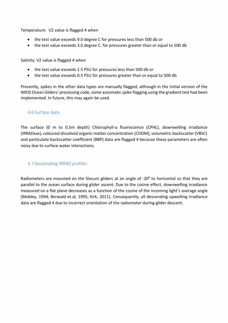
Temperature: V2 value is flagged 4 when
the test value exceeds 9.0 degree C for pressures less than 500 db or
the test value exceeds 3.0 degree C. for pressures greater than or equal to 500 db
Salinity: V2 value is flagged 4 when
the test value exceeds 1.5 PSU for pressures less than 500 db or
the test value exceeds 0.5 PSU for pressures greater than or equal to 500 db Presently, spikes in the other data types are manually flagged, although in the initial version of the IMOS Ocean Gliders’ processing code, some automatic spike flagging using the gradient test had been implemented. In future, this may again be used.
4.6 Surface data
The surface (0 m to 0.5m depth) Chlorophyll-a fluorescence (CPHL), downwelling irradiance
(IRRADxxx), coloured dissolved organic matter concentration (CDOM), volumetric backscatter (VBSC)
and particulate backscatter coefficient (BBP) data are flagged 4 because these parameters are often
noisy due to surface water interactions.
4.7 Descending IRRAD profiles
Radiometers are mounted on the Slocum gliders at an angle of -200 to horizontal so that they are
parallel to the ocean surface during glider ascent. Due to the cosine effect, downwelling irradiance
measured on a flat plane decreases as a function of the cosine of the incoming light’s average angle
(Mobley, 1994; Berwald et.al, 1995; Kirk, 2011). Consequently, all descending upwelling irradiance
data are flagged 4 due to incorrect orientation of the radiometer during glider descent.
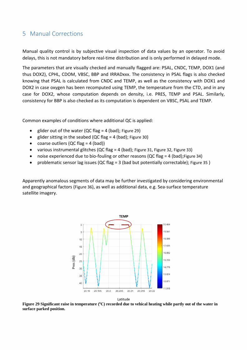
5 Manual Corrections
Manual quality control is by subjective visual inspection of data values by an operator. To avoid
delays, this is not mandatory before real-time distribution and is only performed in delayed mode.
The parameters that are visually checked and manually flagged are: PSAL, CNDC, TEMP, DOX1 (and
thus DOX2), CPHL, CDOM, VBSC, BBP and IRRADxxx. The consistency in PSAL flags is also checked
knowing that PSAL is calculated from CNDC and TEMP, as well as the consistency with DOX1 and
DOX2 in case oxygen has been recomputed using TEMP, the temperature from the CTD, and in any
case for DOX2, whose computation depends on density, i.e. PRES, TEMP and PSAL. Similarly,
consistency for BBP is also checked as its computation is dependent on VBSC, PSAL and TEMP.
Common examples of conditions where additional QC is applied:
glider out of the water (QC flag = 4 (bad); Figure 29)
glider sitting in the seabed (QC flag = 4 (bad); Figure 30)
coarse outliers (QC flag = 4 (bad))
various instrumental glitches (QC flag = 4 (bad); Figure 31, Figure 32, Figure 33)
noise experienced due to bio-fouling or other reasons (QC flag = 4 (bad);Figure 34)
problematic sensor lag issues (QC flag = 3 (bad but potentially correctable); Figure 35 )
Apparently anomalous segments of data may be further investigated by considering environmental and geographical factors (Figure 36), as well as additional data, e.g. Sea-surface temperature satellite imagery.
TEMP
Latitude
Figure 29 Significant raise in temperature (oC) recorded due to vehical heating while partly out of the water in
surface parked position.
Pre
s (d
b)
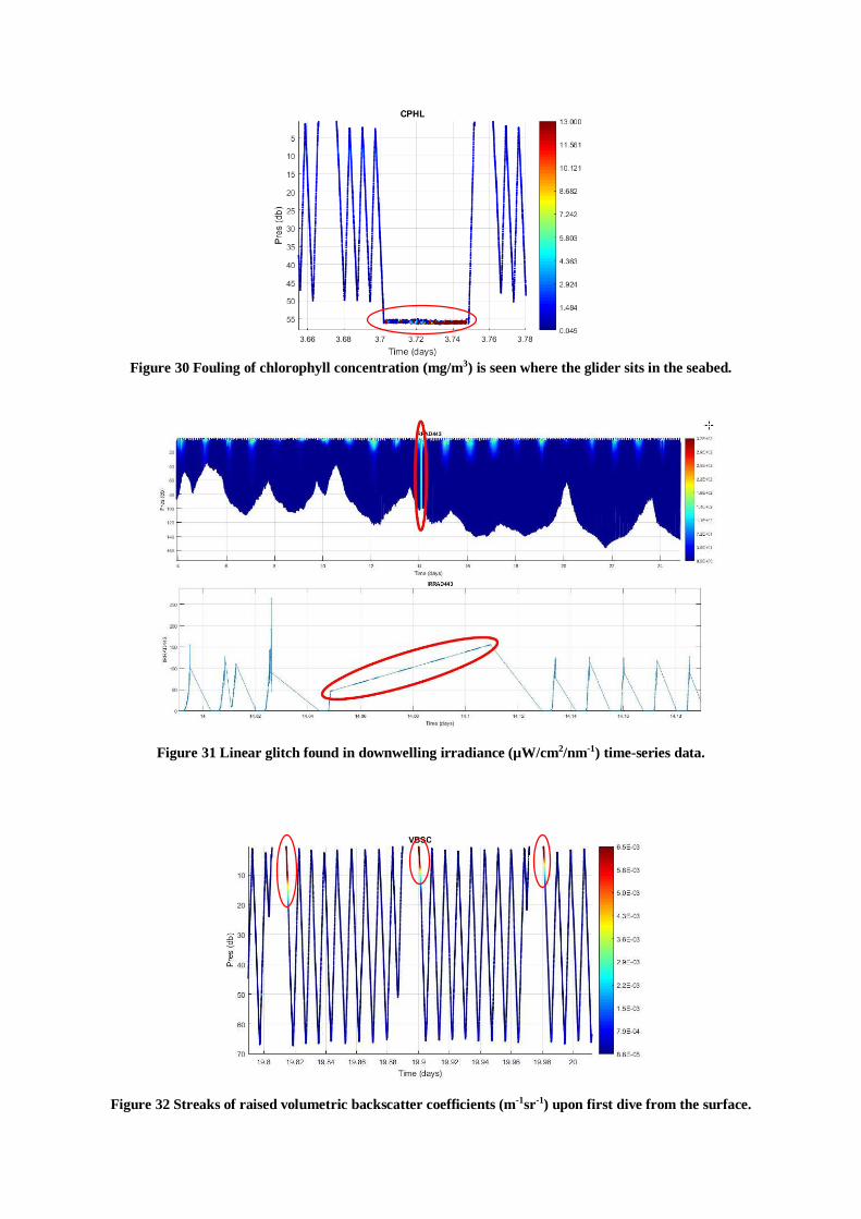
Figure 30 Fouling of chlorophyll concentration (mg/m3) is seen where the glider sits in the seabed.
Figure 31 Linear glitch found in downwelling irradiance (µW/cm2/nm-1) time-series data.
Figure 32 Streaks of raised volumetric backscatter coefficients (m-1sr-1) upon first dive from the surface.
Figure 33 Glitches seen in the vicinity of vehicle inflexion and deflection, in dissolved oxygen concentration
(µmol/kg) data.
Figure 34 Extremely heavy bio-fouling seen in chlorophyll concentration (mg/m3) after 25 days.
Figure 35 Positive and negative spiking (circled) in salinity data that could not be sufficiently resolved by the
present automatic lag correction procedures; these occur especially the interphase between different water types.
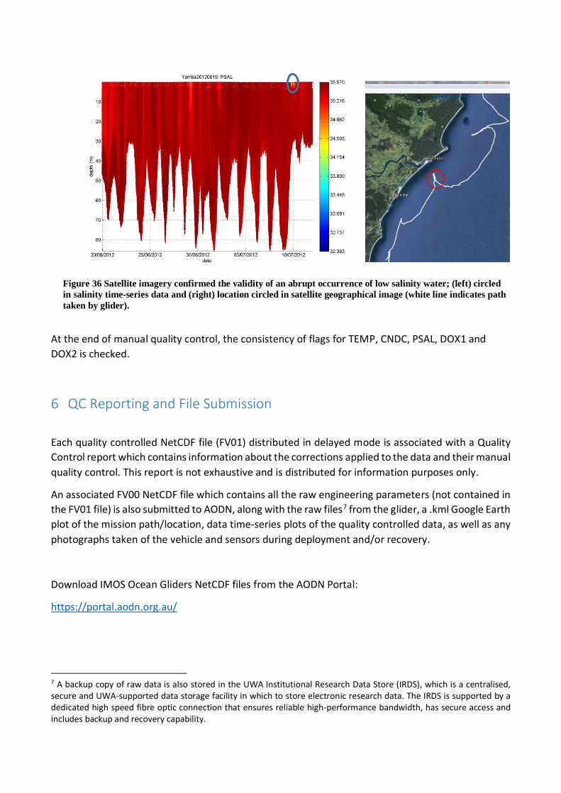
At the end of manual quality control, the consistency of flags for TEMP, CNDC, PSAL, DOX1 and
DOX2 is checked.
6 QC Reporting and File Submission
Each quality controlled NetCDF file (FV01) distributed in delayed mode is associated with a Quality
Control report which contains information about the corrections applied to the data and their manual
quality control. This report is not exhaustive and is distributed for information purposes only.
An associated FV00 NetCDF file which contains all the raw engineering parameters (not contained in
the FV01 file) is also submitted to AODN, along with the raw files7 from the glider, a .kml Google Earth
plot of the mission path/location, data time-series plots of the quality controlled data, as well as any
photographs taken of the vehicle and sensors during deployment and/or recovery.
Download IMOS Ocean Gliders NetCDF files from the AODN Portal:
https://portal.aodn.org.au/
7 A backup copy of raw data is also stored in the UWA Institutional Research Data Store (IRDS), which is a centralised, secure and UWA-supported data storage facility in which to store electronic research data. The IRDS is supported by a dedicated high speed fibre optic connection that ensures reliable high-performance bandwidth, has secure access and includes backup and recovery capability.
Figure 36 Satellite imagery confirmed the validity of an abrupt occurrence of low salinity water; (left) circled
in salinity time-series data and (right) location circled in satellite geographical image (white line indicates path
taken by glider).
7 Data Visualisation Tools
Two data visualisation tools: GLIDERSCOPE and NetCDF Ninja, have been developed for users of
ocean glider data. Both have been designed to install on both Window and Macintosh platforms as
standalone applications. No access to MATLAB software and no coding knowledge is required for
these software to run.
Meanwhile, for the users who do use MATLAB (version R2012b onwards), app versions of both
software are also available for convenient addition to their MATLAB Apps Toolstrip.
Free software downloads available from:
http://imos.org.au/facilities/oceangliders/glider-data/
7.1 GLIDERSCOPE
GLIDERSCOPE is an IMOS Ocean Gliders software package designed to allow users quick and easy
visualisation of ocean glider oceanographic data in NetCDF files from IMOS as well as internationally,
from the U.S. Integrated Ocean Observing System (IOOS) and Everyone's Gliding Observatories (EGO).
Using a convenient graphical user interface, users may load NetCDF files, filter out the bad data and
isolate interesting segments of data either spatially or temporally.
A variety of useful data graphical visualisation techniques can be applied to examine the data, e.g.
plots of water properties viewed in 2D/ 3D space, interpolated contour charts, vertical profile plots
and water properties comparison charts (Figure 38). Moreover, GLIDERSCOPE performs calculations
for additional parameters such as light attenuation coefficient, 1% photic depth, sound velocity and
local time zone, and offers further tools for the manipulation of the appearance of the plots, as well
as a virtual Niskin bottle which may be dropped anywhere in cross-sectional plots so that properties
of that particular parcel of water may instantly be known. Additionally, data may be exported to text
or NetCDF files for later access in other applications.
GLIDERSCOPE download:
http://imos.org.au/facilities/oceangliders/glider-data/gliderscope/
Furthermore, GLIDERSCOPE is supported by
(i) A workshop paper, entitled “Observing the Ocean with Gliders: Techniques for Data
Visualization and Analysis”, published in Oceanography (Hanson et al., 2017).
(ii) GLIDERSCOPE instructional videos, available on The Ocean Society (TOS) channel on
YouTube.
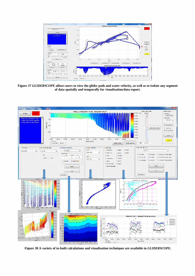
Figure 37 GLIDERSCOPE allows users to view the glider path and water velocity, as well as to isolate any segment
of data spatially and temporally for visualisation/data export.
Figure 38 A variety of in-built calculations and visualisation techniques are available in GLIDERSCOPE.

7.2 NetCDF Ninja
NetCDF Ninja is a NetCDF file browser used for exploring and editing information in not just ocean
glider data NetCDF files, but any NetCDF file. This software was created as an IMOS Ocean Gliders
initiative to complement GLIDERSCOPE. Using NetCDF Ninja, all Global Attributes and Variable
Attributes may be read and edited (Figure 39). Variables may be viewed graphically and individual
data points read/edited. A zoom tool and sample box are also available to allow the user to scrutinise
data more closely and immediately determine the range in any chosen segment of the dataset.
With the advent of the international version of GLIDERSCOPE, users will find that NetCDF files
downloaded from certain overseas repositories sometimes contain errors (e.g. all TIME data are
invalid since all the TIME values exceed the valid_max stated), which make data visualisation
problematic. In such cases, NetCDF Ninja can be used to quickly identify and correct the mistake (e.g.
change the value of valid_max) without any need for coding, so that the user may quickly proceed to
plot and analyse the data.
Figure 39 Dashboard of NetCDF Ninja.
NetCDF Ninja download:
http://imos.org.au/facilities/oceangliders/glider-data/netcdfninja/

Bibliography
Aanderaa (2007). TD 218 Operating Manual Oxygen Optodes.
AODN Portal User Guide; Public Documents (2016). Ocean Gliders - workflow [online] Available at:
https://help.aodn.org.au/public-documents/imos/facilities/workflows/ [Accessed 15 Oct. 2018]
Argo (2013). Argo User’s Manual (Version 3.03).
AUVAC (2018). AUV System Spec Sheet [online] Available at:
http://auvac.org/uploads/configuration/Glider_structure.jpg [Accessed 15 Nov. 2018]
Berwald, J., Stramski, D., Mobley, C.D. and Kiefer, D.A. (1995). Influences of Absorption and Scattering on
Vertical Changes in the Average Cosine of the Underwater Light Field, Limnology and Oceanography, 40,
1347-1357.
Bishop, C.M. (2008). Sensor Dynamics of Autonomous Underwater Gliders, Memorial University of
Newfoundland, Newfoundland, USA.
Boss, E., Pegau, W.S. (2001). Relationship of light scattering at an angle in the backwards direction to the
backscattering coefficient, Applied Optics, 40 (30), 5503-5507.
Cetinic, I., Toro-Farmer, G., Ragan, M., Oberg, C. and Jones, B.H. (2009). Calibration procedure for Slocum
glider deployed optical instruments, Optics Express, 17 (18), 15420 – 15430.
EGO. (2013). EGO User's Manual, Version 1.01.
Farinato, R.S. and Rowell, R. L. (1976). New values of the light scattering depolarization and anisotropy of
water, J. Chem. Phys., 65, 593-595.
Frajka-Williams, E., (2011). Determining Vertical Water Velocities from Seaglider, Journal of Atmospheric and
Oceanic Technology, 28 (12), 1641-1656.
Garau, B., Ruiz, S., Zhang, W., Pascual, A., Heslop, E., Kerfoot, J. and Tintoré, J. (2011). Thermal Lag
Corrections on Slocum CTD Glider Data, Journal of Atmospheric and Oceanic Technology, 28, 1065-1071.
Garcia, H.E. and Gordon, L.I. (1992). Oxygen Solubility in Seawater: Better Fitting Equations, Limnology and
Oceanography, 37 (6), 1307-1312.
Gregg, M.C. and Hess, W.C. (1985). Dynamic Response Calibration of Sea-Bird Temperature and Conductivity
Probes, Journal of Atmospheric and Oceanic Technology, 2, 304-313.
Gourcuff, C, (2014a). ANFOG Slocum CTD data correction, IMOS Australian National Facility for Ocean
Gliders.
Gourcuff, C, (2014b). ANFOG Slocum Oxygen data: new computation, IMOS Australian National Facility for
Ocean Gliders.
Hanson, C., Woo, L.M., Thomson, P. & Pattiaratchi, C. (2017). Observing the Ocean with Gliders: Techniques
for Data Visualization and Analysis, Oceanography, 30 (2), 222-227.
Horne, E.P.W. and Toole, J.M. (1980). Sensor Response Mismatches and Lag Correction Techniques for
Temperature-Salinity Profilers. Journal of Physical Oceanography, 10, 1122-1130.
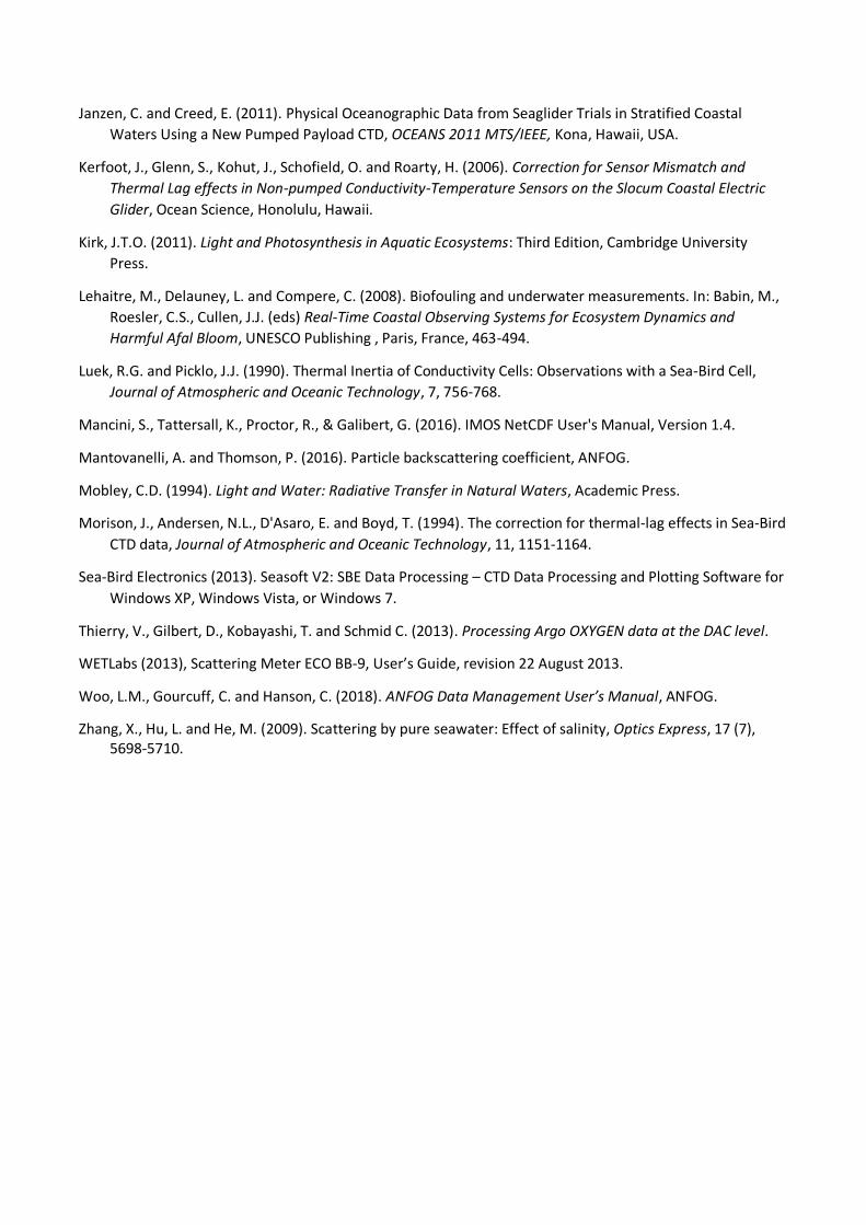
Janzen, C. and Creed, E. (2011). Physical Oceanographic Data from Seaglider Trials in Stratified Coastal
Waters Using a New Pumped Payload CTD, OCEANS 2011 MTS/IEEE, Kona, Hawaii, USA.
Kerfoot, J., Glenn, S., Kohut, J., Schofield, O. and Roarty, H. (2006). Correction for Sensor Mismatch and
Thermal Lag effects in Non-pumped Conductivity-Temperature Sensors on the Slocum Coastal Electric
Glider, Ocean Science, Honolulu, Hawaii.
Kirk, J.T.O. (2011). Light and Photosynthesis in Aquatic Ecosystems: Third Edition, Cambridge University
Press.
Lehaitre, M., Delauney, L. and Compere, C. (2008). Biofouling and underwater measurements. In: Babin, M.,
Roesler, C.S., Cullen, J.J. (eds) Real-Time Coastal Observing Systems for Ecosystem Dynamics and
Harmful Afal Bloom, UNESCO Publishing , Paris, France, 463-494.
Luek, R.G. and Picklo, J.J. (1990). Thermal Inertia of Conductivity Cells: Observations with a Sea-Bird Cell,
Journal of Atmospheric and Oceanic Technology, 7, 756-768.
Mancini, S., Tattersall, K., Proctor, R., & Galibert, G. (2016). IMOS NetCDF User's Manual, Version 1.4.
Mantovanelli, A. and Thomson, P. (2016). Particle backscattering coefficient, ANFOG.
Mobley, C.D. (1994). Light and Water: Radiative Transfer in Natural Waters, Academic Press.
Morison, J., Andersen, N.L., D'Asaro, E. and Boyd, T. (1994). The correction for thermal-lag effects in Sea-Bird
CTD data, Journal of Atmospheric and Oceanic Technology, 11, 1151-1164.
Sea-Bird Electronics (2013). Seasoft V2: SBE Data Processing – CTD Data Processing and Plotting Software for
Windows XP, Windows Vista, or Windows 7.
Thierry, V., Gilbert, D., Kobayashi, T. and Schmid C. (2013). Processing Argo OXYGEN data at the DAC level.
WETLabs (2013), Scattering Meter ECO BB-9, User’s Guide, revision 22 August 2013.
Woo, L.M., Gourcuff, C. and Hanson, C. (2018). ANFOG Data Management User’s Manual, ANFOG.
Zhang, X., Hu, L. and He, M. (2009). Scattering by pure seawater: Effect of salinity, Optics Express, 17 (7), 5698-5710.