Chapter 5: Multivariate Analysis and Repeated Measuresutstat.toronto.edu/~brunner/oldclass/429Fall04/text/Ch5.pdf · Chapter 5: Multivariate Analysis and Repeated Measures M u lll

Chapter 5: Multivariate Analysis and RepeatedMeasures

MMMMuuuullllttttiiiivvvvaaaarrrriiiiaaaatttteeee -- More than one dependent variable at once. Why do it? Primarilybecause if you do parallel analyses on lots of outcome measures, the probability ofgetting significant results just by chance will definitely exceed the apparent å = 0.05level. It is also possible in principle to detect results from a multivariate analysis thatare not significant at the univariate level.

The simplest way to do multivariate analysis is to do a univariate analysis on eachdependent variable separately, and apply a Bonferroni correction. The disadvantage isthat testing this way is less powerful than doing it with real multivariate tests.

Another advantage of a true multivariate analysis is that it can "notice" things missed byseveral Bonferroni-corrected univariate analyses, because ...

Under the surface, a classical multivariate analysis involves the construction of theunique linear combination of the dependent variables that shows the strongestrelationship (in the sense explaining the remaining variation) with the independentvariables.

The linear combination in question is called the first ccccaaaannnnoooonnnniiiiccccaaaallll vvvvaaaarrrriiiiaaaatttteeee or ccccaaaannnnoooonnnniiiiccccaaaallllvvvvaaaarrrriiiiaaaabbbblllleeee.

The number of canonical variables equals the number of dependent variables (or IVs, whichever is fewer).

The canonical variables are all uncorrelated with each other. The second one is constructed so that it has as strong a relationship as possible to the independent variables -- subject to the constraint that it have zero correlation with the first one, and so on.

Chapter 5, Page 1

This why it is not optimal to do a principal components analysis (or factor analysis) on a set of dependent variables, and then treat the components (or factor scores) as dependent variables. Ordinary multivariate analysis is already doing this, and doing it much better.

AAAAssssssssuuuummmmppppttttiiiioooonnnnssss

As in the case of univariate analysis, the statistical assumptions of multivariate analysisconcern conditional distributions -- conditional upon various configurations ofindependent variable XXXX values. Here we are talking about the conditional jointdistribution of several dependent variables observed for each case, say Y1, ..., Yk.These are often described as a "vector" of observations. It may help to think of thecollection of DV values for a case as a point in k-dimensional space, and to imagine anarrow pointing from the origin (0, ...,0) to the point (Y1, ..., Yk); the arrow is literallya vector. As I say, this may help. Or it may not.

The classical assumptions of multivariate analysis depend on the idea of a populationcovariance. The population covariance between Y2 and Y4 is denoted ß2,4, and isdefined by ß2,4 = ß2 ß4, where

ß2 is the population standard deviation of Y2, ß4 is the population standard deviation of Y4, and is the population correlation between Y2 and Y4

(that's the Greek letter rho).

The population covariance can be estimated by the sample covariance, defined in aparallel way by s2,4 = r s2 s4, where s2 and s4 are the sample standard deviationsand r is the Pearson correlation coefficient.

Whether we are talking about population parameters or sample statistics, it is clear thatzero covariance means zero correlation and vice versa.

Chapter 5, Page 2

We will use Í (the capital Greek letter sigma) to stand for the population variance-covariance matrix. This is a k by k rectangular array of numbers with variances onthe main diagonal, and covariances on the off-diagonals. For 4 dependent variables itwould look like this:

S =

s1

2 s1,2 s1,3 s1,4

s1,2 s22 s2,3 s2,4

s1,3 s2,3 s32 s3,4

s1,4 s2,4 s3,4 s42

With this background, the assumptions of classical multivariate analysis are that(conditional on the X values)

Sample vectors Y = (Y1, ..., Yk) represent independent observations

for different cases.

Each conditional distribution is multivariate normal.

Each conditional distribution has the same population variance-covariance matrix Í.

These assumptions are directly parallel to those of classical univariate regression.Also parallel to univariate analysis is a linear model for each population mean(now we have k of them).

Chapter 5, Page 3

E[Y|x] =

m1

m2

mk

=

E[Y1|x]E[Y2|x]

E[Yk|x]

=

b0,1 + b1,1x1 + + bp ± 1,1xp ± 1

b0,2 + b1,2x1 + + bp ± 1,2xp ± 1

b0,k + b1,kx1 + + bp ± 1,kxp ± 1

There are k different sets of regression coefficients -- one for each dependentvariable.

There is only one set of independent variables -- the same for each DV.Dummy variables, interactions etc. are exactly as in univariate regression.

Estimation: The least squares estimates of those doubly-subscripted betas areexactly what one would get from k separate univariate analyses. Since theestimated regression coefficients are the same, so are the Yô values and so are theresiduals. All methods for univariate residual analysis apply.

Only the tests and confidence intervals (probability statements) are different forunivariate and multivariate analysis.

Testing: In univariate analysis, different standard methods for deriving tests(these are hidden from you) all point to Fisher's F test. In multivariate analysisthere are four major test statistics, Wilks' Lambda, Pillai's Trace, theHotelling-Lawley Trace, and Roy's Greatest Root.

Chapter 5, Page 4

When there is only one dependent variable, these are all equivalent to F. Whenthere is more than one DV they are all about equally "good" (in any reasonablesense), and conclusions from them generally agree -- but not always. Sometimesone will designate a finding as significant and another will not. In this case youhave borderline results and there is no conventional way out of the dilemma.

The four multivariate test statistics all have F approximations that are used bySAS and other stat packages to compute p-values. Tables are available intextbooks on multivariate analysis. For the first three tests (Wilks' Lambda,

Pillai's Trace and the Hotelling-Lawley Trace), the F approximations are verygood. For Roy's greatest root the F approximation is lousy. This is a problemwith the cheap method for getting p-values, not with the test itself. One canalways use tables.

When a multivariate test is significant, many people then follow up with ordinaryunivariate tests to see "which dependent variable the results came from." Moreconservative (and better) is to follow up with Bonferroni-corrected univariatetests. When you do this, there is no guarantee that any of the Bonferroni-corrected tests will be significant.

It is also possible, and in some ways very appealing, to follow up a significantmultivariate test with Scheffe tests. For example, Scheffe follow-ups to asignificant one-way multivariate ANOVA would include adjusted versions of allthe corresponding univariate one-way ANOVAs, all multivariate pairwisecomparisons, all univariate pairwise comparisons, and lots of other possibilities–– all simultaneously protected at the 0.05 level.

You can also try interpret a significant multivariate effect by looking at thecanonical variates, but there is no guarantee they will make sense.

Chapter 5, Page 5

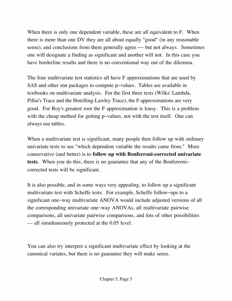
/******************** senicmv96a.sas *************************/options linesize=79;title 'Senic data: SAS glm & reg multivariate intro';

%include 'senicdef.sas'; /* senicdef.sas reads data, etc. Includes reg1-reg3, ms1 & mr1-mr3 */

/* First a nice two-factor MANOVA on infrisk & stay */

proc glm; class region medschl; model infrisk stay = region|medschl; manova h = _all_;

The glm output starts with full univariate output for each DV. Then (for eacheffect tested) some multivariate output you ignore,

General Linear Models Procedure Multivariate Analysis of Variance

Characteristic Roots and Vectors of: E Inverse * H, where H = Type III SS&CP Matrix for REGION E = Error SS&CP Matrix

Characteristic Percent Characteristic Vector V'EV=1 Root INFRISK STAY

0.14830859 95.46 -0.00263408 0.06067199 0.00705986 4.54 0.08806967 -0.03251114

Followed by the interesting part.

Manova Test Criteria and F Approximations for the Hypothesis of no Overall REGION Effect H = Type III SS&CP Matrix for REGION E = Error SS&CP Matrix

S=2 M=0 N=51

Statistic Value F Num DF Den DF Pr > F

Wilks' Lambda 0.86474110 2.6127 6 208 0.0183 Pillai's Trace 0.13616432 2.5570 6 210 0.0207 Hotelling-Lawley Trace 0.15536845 2.6672 6 206 0.0163 Roy's Greatest Root 0.14830859 5.1908 3 105 0.0022

NOTE: F Statistic for Roy's Greatest Root is an upper bound. NOTE: F Statistic for Wilks' Lambda is exact.

Chapter 5, Page 6

. . .

Manova Test Criteria and Exact F Statistics for the Hypothesis of no Overall MEDSCHL Effect H = Type III SS&CP Matrix for MEDSCHL E = Error SS&CP Matrix

S=1 M=0 N=51



NOTE: F Statistic for Roy's Greatest Root is an upper bound.

. . .

Manova Test Criteria and F Approximations for the Hypothesis of no Overall REGION*MEDSCHL Effect H = Type III SS&CP Matrix for REGION*MEDSCHL E = Error SS&CP Matrix

S=2 M=0 N=51




Remember the output started with the univariate analyses. We'll look at themhere (out of order) -- just Type III SS, because that's parallel to the multivariatetests. We are tracking down the significant multivariate effects for Region andMedical School Affiliation. Using Bonferroni correction means only believe it ifp < 0.025.

Dependent Variable: INFRISK prob of acquiring infection in hospital

Source DF Type III SS Mean Square F Value Pr > F

REGION 3 6.61078342 2.20359447 1.35 0.2623MEDSCHL 1 6.64999500 6.64999500 4.07 0.0461REGION*MEDSCHL 3 5.32149160 1.77383053 1.09 0.3581

Chapter 5, Page 7

Dependent Variable: STAY av length of hospital stay, in days


REGION 3 41.61422755 13.87140918 5.19 0.0022MEDSCHL 1 22.49593643 22.49593643 8.41 0.0045REGION*MEDSCHL 3 0.92295998 0.30765333 0.12 0.9511

We conclude that the multivariate effect comes from a univariate relationshipbetween the IVs and stay. Question: If this is what we were going to do in theend, why do a multivariate analysis at all? Why not just two univariate analyseswith a Bonferroni correction?

The command file senicmv96a.sas continues as follows;

/* Now do it with proc reg. Syntax is the same, except list more than one dependent variable, and say "mtest" instead of "test." */

proc reg; model infrisk stay = reg1-reg3 ms1 mr1-mr3; regtest: mtest reg1=reg2=reg3=0; mstest: mtest ms1=0; m_by_r: mtest mr1=mr2=mr3=0;

This gives us exactly the same results we got from proc glm. The point is thatmultivariate analysis of variance is just a special case of multivariate regression;you can do it either way. Proc reg can give you a little more control over thedetails, but at the cost of setting up your own dummy variables.

Chapter 5, Page 8

Repeated measures

In certain kinds of experimental research, it is common to obtain repeatedmeasurements of a variable from the same individual at several different

points in time. Usually it is unrealistic to assume that these repeatedobservations are uncorrelated, and it is very desirable to build their inter-correlations into the statistical model.

Sometimes, an individual (in some combination of experimental conditions) ismeasured under essentially the same conditions at several different points in time.In that case we will say that time is a within-subjects factor, because each subjectcontributes data at more than one value of the IV "time." If a subject experiencesonly one value of an IV, it is called a between subjects factor.

.Sometimes, an individual (in some combination of other experimentalconditions) experiences more than one experimental treatment -- for examplejudging the same stimuli under different background noise levels. In this case theorder of presentation of different noise levels would be counterbalanced so thattime and noise level are unrelated (not confounded). Here noise level would be awithin-subjects factor. The same study can definitely have more than onewithin-subjects factor and more than one between subjects factor.

The meaning of main effects and interactions, as well as their graphicalpresentation, is the same for within and between subjects factors.

We will discuss three methods for analyzing repeated measures data. In an orderthat is convenient but not chronological they are

1. The multivariate approach.2. The classical univariate approach.3. The covariance structure approach.

Chapter 5, Page 9

The multivariate approach to repeated measures

First, note that any of the 3 methods can be multivariate, in the sense that severaldependent variables can be measured at more than one time point. We will startwith the simpler case in which a single dependent variable is measured for eachsubject on several different occasions.

The basis of the multivariate approach to repeated measures is that the differentmeasurements conducted on each individual should be considered as

multiple dependent variables.

If there are k dependent variables, regular multivariate analysis allows for theanalysis of up to k linear combinations of those DVs, instead of the originaldependent variables.

All the multivariate approach does is to set up those linear combinations to bemeaningful in terms of representing the repeated measures structure of the data.

For example, suppose that men and women in 3 different age groups are tested ontheir ability to detect a signal under 5 different levels of background noise.There are 10 women and 10 men in each age group for a total n = 60. Order ofpresentation of noise levels is randomized for each subject, and the subjectsthemselves are tested in random order. This is a three-factor design. Age andsex are between subjects factors, and noise level is a within-subjects factor.

Let Y1, Y2, Y3, Y4 and Y5 be the "Detection Scores" under the 5 different noiselevels.

Chapter 5, Page 10

Let Y1, Y2, Y3, Y4 and Y5 be the "Detection Scores" under the 5 different noiselevels. Their population means are µ1, µ2, µ3, µ4 and µ5 respectively.

Now construct 5 linear combinations of the Y's, as follows.

W1 = (Y1+Y2+Y3+Y4+Y5 ) / 5 E(W1) = (µ1+µ2+µ3+µ4+µ5 ) / 5W2 = Y1 - Y2 E(W2) = µ1 - µ2W3 = Y2 - Y3 E(W3) = µ2 - µ3W4 = Y3 - Y4 E(W4) = µ3 - µ4W5 = Y4 - Y5 E(W5) = µ4 - µ5

All the population means are of course conditional on the values of someindependent variables. We will adopt a linear model for each one, as in the usualmultivariate setup. In this case the independent variables (the weights for thelinear combinations of ∫'s) are dummy variables for the categorical independentvariables sex & age, and the product terms for their interactions.

Between-subjects effects: The main effects for age and sex, and the age by sexinteraction, are just analyses conducted as usual on a single linear combination ofthe DVs, that is, on W1. This is what we want; we are just averaging acrosswithin-subject values.

Within-subject effects: Suppose that (for each configuration of X values)

E(W2) = E(W2) = E(W2) = E(W2) = 0This means µ1 = µ2, µ2 = µ3, µ3 = µ4, µ4 = µ5.

That is, no difference among noise level means, i.e., no main effect for thewithin-subjects factor.

Chapter 5, Page 11

Interactions of between and within-subjects factors are between-subjectseffects tested simultaneously on the dependent variables representing

differences among within-subject values -- W2 through W5 in this case. Forexample, a significant sex difference in W2 through W5 means that the pattern ofdifferences in mean discrimination among noise levels is different for males andfemales. Conceptually, this is exactly a noise level by sex interaction.

Similarly, a sex by age interaction on W2 through W5 simultaneously means thatthe pattern of differences in mean discrimination among noise levels depends onspecial combinations of age and sex -- a three-way (age by sex by noise)interaction.

Note: There is nothing in this discussion that limits us to dummy variables forcategorical independent variables. Thus, multiple regression with repeatedmeasures is completely reasonable and presents no special difficulties.

Here is noise.dat. Order of vars is

ident, interest, sex, age, noise level, time noise level presented, discrim score

esc> less noise.dat 1 2.5 1 2 1 4 50.7 1 2.5 1 2 2 1 27.4 1 2.5 1 2 3 3 39.1 1 2.5 1 2 4 2 37.5 1 2.5 1 2 5 5 35.4 2 1.9 1 2 1 3 40.3 2 1.9 1 2 2 1 30.1 2 1.9 1 2 3 5 38.9 2 1.9 1 2 4 2 31.9 2 1.9 1 2 5 4 31.6 3 1.8 1 3 1 2 39.0 3 1.8 1 3 2 5 39.1 3 1.8 1 3 3 4 35.3 3 1.8 1 3 4 3 34.8 3 1.8 1 3 5 1 15.4 4 2.2 0 1 1 2 41.5 4 2.2 0 1 2 4 42.5

Chapter 5, Page 12

/**************** noise96a.sas ***********************/options linesize=79 pagesize=250;title 'Repeated measures on Noise data: Multivariate approach';proc format; value sexfmt 0 = 'Male' 1 = 'Female' ;

data loud; infile 'noise.dat'; /* Multivariate data read */ input ident interest sex age noise1 time1 discrim1 ident2 inter2 sex2 age2 noise2 time2 discrim2 ident3 inter3 sex3 age3 noise3 time3 discrim3 ident4 inter4 sex4 age4 noise4 time4 discrim4 ident5 inter5 sex5 age5 noise5 time5 discrim5 ; format sex sex2-sex5 sexfmt.; /* noise1 = 1, ... noise5 = 5. time1 = time noise 1 presented etc. ident, interest, sex & age are identical on each line */ label interest = 'Interest in topic (politics)';

proc glm; class age sex; model discrim1-discrim5 = age|sex; repeated noise profile/ short summary;

First we get univariate analyses of discrim1-discrim5 -- not the transformedvars yet. Then,

General Linear Models Procedure Repeated Measures Analysis of Variance Repeated Measures Level Information

Dependent Variable DISCRIM1 DISCRIM2 DISCRIM3 DISCRIM4 DISCRIM5

Level of NOISE 1 2 3 4 5

Manova Test Criteria and Exact F Statistics for the Hypothesis of no NOISE Effect H = Type III SS&CP Matrix for NOISE E = Error SS&CP Matrix

S=1 M=1 N=24.5



Manova Test Criteria and F Approximations for

Chapter 5, Page 13

the Hypothesis of no NOISE*AGE Effect H = Type III SS&CP Matrix for NOISE*AGE E = Error SS&CP Matrix

S=2 M=0.5 N=24.5




Manova Test Criteria and Exact F Statistics for the Hypothesis of no NOISE*SEX Effect H = Type III SS&CP Matrix for NOISE*SEX E = Error SS&CP Matrix

S=1 M=1 N=24.5



Manova Test Criteria and F Approximations for the Hypothesis of no NOISE*AGE*SEX Effect H = Type III SS&CP Matrix for NOISE*AGE*SEX E = Error SS&CP Matrix

S=2 M=0.5 N=24.5




Chapter 5, Page 14

General Linear Models Procedure Repeated Measures Analysis of Variance Tests of Hypotheses for Between Subjects Effects


AGE 2 1751.814067 875.907033 5.35 0.0076SEX 1 77.419200 77.419200 0.47 0.4946AGE*SEX 2 121.790600 60.895300 0.37 0.6911

Error 54 8839.288800 163.690533

Then we are given "Univariate Tests of Hypotheses for Within Subject Effects"We will discuss these later. After that in the lst file, ...

Repeated measures on Noise data: Multivariate approach

General Linear Models Procedure Repeated Measures Analysis of Variance Analysis of Variance of Contrast Variables

NOISE.N represents the nth successive difference in NOISE

Contrast Variable: NOISE.1


MEAN 1 537.00416667 537.00416667 5.40 0.0239AGE 2 10.92133333 5.46066667 0.05 0.9466SEX 1 45.93750000 45.93750000 0.46 0.4996AGE*SEX 2 83.67600000 41.83800000 0.42 0.6587

Error 54 5370.09100000 99.44612963




Error 54 5569.94700000 103.14716667

Chapter 5, Page 15




Error 54 3802.61800000 70.41885185




Error 54 3602.36600000 66.71048148

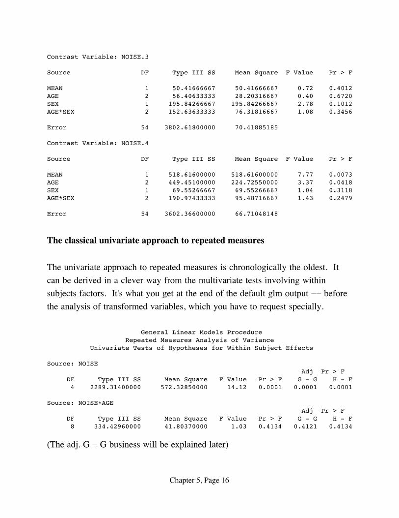
The classical univariate approach to repeated measures

The univariate approach to repeated measures is chronologically the oldest. Itcan be derived in a clever way from the multivariate tests involving withinsubjects factors. It's what you get at the end of the default glm output -- beforethe analysis of transformed variables, which you have to request specially.

General Linear Models Procedure Repeated Measures Analysis of Variance Univariate Tests of Hypotheses for Within Subject Effects

Source: NOISE Adj Pr > F DF Type III SS Mean Square F Value Pr > F G - G H - F 4 2289.31400000 572.32850000 14.12 0.0001 0.0001 0.0001

Source: NOISE*AGE Adj Pr > F DF Type III SS Mean Square F Value Pr > F G - G H - F 8 334.42960000 41.80370000 1.03 0.4134 0.4121 0.4134

(The adj. G - G business will be explained later)

Chapter 5, Page 16

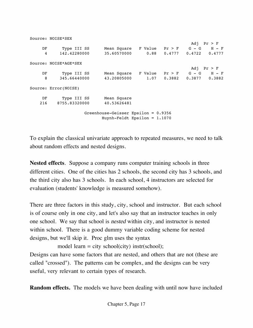
Source: NOISE*SEX Adj Pr > F DF Type III SS Mean Square F Value Pr > F G - G H - F 4 142.42280000 35.60570000 0.88 0.4777 0.4722 0.4777

Source: NOISE*AGE*SEX Adj Pr > F DF Type III SS Mean Square F Value Pr > F G - G H - F 8 345.66440000 43.20805000 1.07 0.3882 0.3877 0.3882

Source: Error(NOISE)

DF Type III SS Mean Square 216 8755.83320000 40.53626481

Greenhouse-Geisser Epsilon = 0.9356 Huynh-Feldt Epsilon = 1.1070

To explain the classical univariate approach to repeated measures, we need to talkabout random effects and nested designs.

Nested effects. Suppose a company runs computer training schools in threedifferent cities. One of the cities has 2 schools, the second city has 3 schools, andthe third city also has 3 schools. In each school, 4 instructors are selected forevaluation (students' knowledge is measured somehow).

There are three factors in this study, city, school and instructor. But each schoolis of course only in one city, and let's also say that an instructor teaches in onlyone school. We say that school is nested within city, and instructor is nestedwithin school. There is a good dummy variable coding scheme for nesteddesigns, but we'll skip it. Proc glm uses the syntax

model learn = city school(city) instr(school);Designs can have some factors that are nested, and others that are not (these arecalled "crossed"). The patterns can be complex, and the designs can be veryuseful, very relevant to certain types of research.

Random effects. The models we have been dealing with until now have included

Chapter 5, Page 17

only fixed effects. In a random effects model, the values of the independentvariable represent a random sample from some population of values. In thecomputer school example, if instructors were just designated for inclusion in thestudy, instructor would be a fixed effect (we are comparing Chris to Pat). If theywere randomly sampled from a population of instructors (this is a big company),instructor would be a random effect. A model that contains both fixed andrandom effects is called "mixed."

Significance tests in random and mixed models use F statistics, but thedenominator is not always MSE, as it is for purely fixed effects models.Sometimes it is an interaction term. Choosing the right error term for mixedmodels can be complicated job, guided by expected values of the mean square(SS/df) terms; these are called expected mean squares. Sometimes there is noright error term and certain hypotheses are untestable with this technology.Fortunately the whole process can be automated, and SAS does a good job. When the design is unbalanced, usually none of the error terms is useful, and

the expected mean squares approach breaks down.

Random effects, like fixed effects, can either be nested or not; it depends on thelogic of the design. An interesting case of nested and purely random effects isprovided by sub-sampling. For example, we take a random sample of towns,from each town we select a random sample of households, and from eachhousehold we select a random sample of individuals to test, or measure, orquestion.

In such cases the population variance of the DV can truly be partitioned intopieces -- the variance due to towns, the variance due to households within towns,and the variance due to individuals within households. These components ofvariance can be estimated, and they are, by a program called proc nested, aspecialized tool for just exactly this design. All effects are random, and each isnested within the preceding one.

Chapter 5, Page 18

Another example: Suppose we are studying waste water treatment, specificallythe porosity of "flocks," nasty little pieces of something floating in the tanks. Werandomly select a sample of flocks, and then cut each one up into very thin slices.We then randomly select a sample of slices (called "sections") from each flock,look at it under a microscope, and assign a number representing how porous it is(how much empty space there is in a designated region of the section). Theindependent variables are flock and section. The research question is whethersection is explaining a significant amount of the variance in porosity -- becauseif not, we can use just one section per flock, and save considerable time &expense.

The SAS syntax for this would be

proc sort; by flock section; /* Data must be sorted */

proc nested;

class flock section;

var por;

The F tests on the output are easy to locate. The last column of output ("Percentof total") is estimated percent of total variance due to the effect. It's fairly closeto R2, but not the same. To include a covariate (say "window"), just usevar window por; instead of var por;. You'll get an analysis of por withwindow as the covariate (which is what you want) and an analysis of window withpor as the covariate (which you should ignore).

Anyway, the classical univariate approach to repeated measures is to treat"subjects" as a random effect that is nested within the between-subjects

factors, and which does not interact with any other factors. Interactionsbetween subjects and various factors may be formally computed, but actuallythese are error terms; they are not tested.

In the noise level example, we could do

Chapter 5, Page 19

/**************** noise96b.sas ***********************/options linesize=79 pagesize=250;title 'Repeated measures on Noise data: Univariate approach';proc format; value sexfmt 0 = 'Male' 1 = 'Female' ;

data loud; infile 'noise.dat'; /* Univariate data read */ input ident interest sex age noise time discrim ; format sex sexfmt.; label interest = 'Interest in topic (politics)' time = 'Order of presenting noise level';

proc glm; class age sex noise ident; model discrim = ident(age*sex) age|sex|noise; random ident(age*sex) / test;

Notice the univariate data read! We are assuming n = number of observations,not number of cases.

The results are identical to the univariate output produced as a by-product of themultivariate approach to repeated measures -- if you know where to look.

The overall test, and tests associated with Type I & Type III SS are all invalid.

There are expected mean squares, which you should probably ignore.

There are also repeated warnings that "This test assumes one or moreother fixed effects are zero." SAS is buying testability of the hypothesesby assuming that you're only interested in an effect if all the higher-orderinteractions involving the effect are absent.

Why do it this way at all? Time-varying covariates.

The univariate approach to repeated measures has some real virtues, sometimes.

Chapter 5, Page 20

Because n = the number of observations rather than the number of cases, it ispossible to have more parameters in a model than cases, or even moremeasurements than cases. In this situation the multivariate approach just blowsup.

(Statistical methods should not be a Procrustean bed.)

The univariate approach may assume n is the number of observations, but it doesnot assume those observations are independent. In fact, the observations thatcome from the same subject are assumed to be correlated, as follows.

The "random effect" for subjects is a little piece of random error, characteristicof an individual. We think of it as random because the individual was randomlysampled from a population. If, theoretically, the only reason that themeasurements from a case are correlated is that each one is affected by this samelittle piece of under-performance or over-performance, the univariate approachrepresents a very good model.

The "random effect for a subject" idea implies a variance-covariance matrix ofthe DVs (say Y1, ..., Y4) with a compound symmetry structure.

S =

s2 + s1 s1 s1 s1

s1 s2 + s1 s1 s1

s1 s1 s2 + s1 s1

s1 s1 s1 s2 + s1

Actually, compound symmetry is sufficient but not necessary for the univariaterepeated F tests to be valid. All that's necessary is "sphericity," which means thecovariances of all differences among Y's within a case are the same.

Chapter 5, Page 21

Another virtue of the univariate approach is that it allows time-dependentcovariates. Standard multivariate analysis has the same X values for eachdependent variable.

Now some weak points of the classical univariate approach:

The model is good if the only reason for correlation among the repeatedmeasures is that one little piece of individuality added to each measurement by asubject. However, if there are other sources of covariation among the repeatedmeasures (like learning, or fatigue, or memory of past performance), there is toomuch chance rejection of the null hypothesis. In this case the multivariateapproach, with its unknown variance-covariance matrix, is more conservative.

Even more conservative (overly so, if the assumptions of the multivariateapproach are met) is the Greenhouse-Geisser correction, which compensates forthe problem by reducing the error degrees of freedom.

If the design is unbalanced (non-proportional n's), the "F-tests" of the classicalunivariate approach do not have an F distribution (even if all the statisticalassumptions are satisfied), and it is unclear what they mean, if anything.

Like the multivariate approach, the univariate approach to repeated measuresanalysis throws out a case if any of the observations are missing. Did somebodysay "mean substitution?" Oh no!)

It has real trouble with unequally spaced observations, and with very natural andhigh quality data sets where (probably) different numbers of observations arecollected for each individual.

Chapter 5, Page 22

The covariance structure approach to repeated measures.

In the covariance structure approach, the data are set up to be read in a univariatemanner, and one of the variables is a case identification, which will be used todetermine which observations of a variable come from the same case. Naturally,data lines from the same case should be adjacent in the file.

Instead of assuming independence or inducing compound symmetry withinsubjects by random effects assumptions, one directly specifies the structure ofthe covariance matrix of the observations that come from the same subject.

The following present no problem at all:

Time-varying covariates (categorical, too)Unbalanced designsUnequally spaced observations*Missing or unequal numbers of observations within subjects*More variables than subjects (but not more parameters than subjects)

It's implemented with SAS proc mixed. Only SAS seems to have it.

∑ Lots of different covariance structures are possible, including compound symmetry and unknown.

∑ A good number of powerful features will not be discussed here.∑ Everything's still assumed multivariate normal.

* Provided this is unrelated to the variable being repeatedly measured. Like ifthe DV is how sick a person is, and the data might be missing because the personis too sick to be tested, there is a problem.

Chapter 5, Page 23

/**************** noise96c.sas ***********************/options linesize=79 pagesize=250;title 'Repeated measures on Noise data: Cov Struct Approach';proc format; value sexfmt 0 = 'Male' 1 = 'Female' ;


proc mixed method = ml; class age sex noise; model discrim = age|sex|noise; repeated / type = un subject = ident r; lsmeans age noise;

proc mixed method = ml; class age sex noise; model discrim = age|sex|noise; repeated / type = cs subject = ident r;

Now part of noise95c.lst

The MIXED Procedure

Class Level Information

Class Levels Values

AGE 3 1 2 3 SEX 2 Female Male NOISE 5 1 2 3 4 5

ML Estimation Iteration History

Iteration Evaluations Objective Criterion

0 1 1521.4783527 1 1 1453.7299937 0.00000000

Convergence criteria met.

Chapter 5, Page 24

R Matrix for Subject 1

Row COL1 COL2 COL3 COL4 COL5

1 54.07988333 17.08300000 21.38658333 17.91785000 24.27668333 2 17.08300000 69.58763333 15.56748333 29.98861667 21.71448333 3 21.38658333 15.56748333 54.37978333 25.15906667 21.00126667 4 17.91785000 29.98861667 25.15906667 59.31531667 27.58265000 5 24.27668333 21.71448333 21.00126667 27.58265000 55.88941667

Covariance Parameter Estimates (MLE)

Cov Parm Estimate Std Error Z Pr > |Z|

DIAG UN(1,1) 54.07988333 9.87359067 5.48 0.0001 UN(2,1) 17.08300000 8.22102992 2.08 0.0377 UN(2,2) 69.58763333 12.70490550 5.48 0.0001 UN(3,1) 21.38658333 7.52577602 2.84 0.0045 UN(3,2) 15.56748333 8.19197469 1.90 0.0574 UN(3,3) 54.37978333 9.92834467 5.48 0.0001 UN(4,1) 17.91785000 7.66900119 2.34 0.0195 UN(4,2) 29.98861667 9.15325956 3.28 0.0011 UN(4,3) 25.15906667 8.01928166 3.14 0.0017 UN(4,4) 59.31531667 10.82944565 5.48 0.0001 UN(5,1) 24.27668333 7.75870531 3.13 0.0018 UN(5,2) 21.71448333 8.52518917 2.55 0.0109 UN(5,3) 21.00126667 7.61610965 2.76 0.0058 UN(5,4) 27.58265000 8.24206793 3.35 0.0008 UN(5,5) 55.88941667 10.20396474 5.48 0.0001 Residual 1.00000000 . . .

Model Fitting Information for DISCRIM

Description Value

Observations 300.0000 Variance Estimate 1.0000 Standard Deviation Estimate 1.0000 Log Likelihood -1002.55 Akaike's Information Criterion -1017.55 Schwarz's Bayesian Criterion -1045.32 -2 Log Likelihood 2005.093 Null Model LRT Chi-Square 67.7484 Null Model LRT DF 14.0000 Null Model LRT P-Value 0.0000

Chapter 5, Page 25

Tests of Fixed Effects

Source NDF DDF Type III F Pr > F

AGE 2 54 5.95 0.0046 SEX 1 54 0.53 0.4716 AGE*SEX 2 54 0.41 0.6635 NOISE 4 216 18.07 0.0001 AGE*NOISE 8 216 1.34 0.2260 SEX*NOISE 4 216 0.99 0.4146 AGE*SEX*NOISE 8 216 1.30 0.2455

From the multivariate approach we had F = 5.35, p < .001 for age & approx F =15.36 for noise.

Least Squares Means

Level LSMEAN Std Error DDF T Pr > |T|

AGE 1 38.66100000 1.21376060 54 31.85 0.0001 AGE 2 35.24200000 1.21376060 54 29.04 0.0001 AGE 3 32.76700000 1.21376060 54 27.00 0.0001 NOISE 1 39.82166667 0.94938474 216 41.94 0.0001 NOISE 2 36.83000000 1.07693727 216 34.20 0.0001 NOISE 3 35.30166667 0.95201351 216 37.08 0.0001 NOISE 4 34.38500000 0.99427793 216 34.58 0.0001 NOISE 5 31.44500000 0.96513744 216 32.58 0.0001

Now for the second mixed run we get the same kind of beginning, and then forcompound symmetry structure,



AGE 2 54 5.95 0.0046 SEX 1 54 0.53 0.4716 AGE*SEX 2 54 0.41 0.6635 NOISE 4 216 15.69 0.0001 AGE*NOISE 8 216 1.15 0.3338 SEX*NOISE 4 216 0.98 0.4215 AGE*SEX*NOISE 8 216 1.18 0.3096

From the univariate approach we had F = 14.12 for noise.

Chapter 5, Page 26

Now proc glm will allow easy examination of residuals no matter which approachyou take to repeated measures, provided the data are read in a univariate manner.

/**************** noise96d.sas ***********************/options linesize=79 pagesize=60;title 'Repeated measures on Noise data: Residuals etc.';proc format; value sexfmt 0 = 'Male' 1 = 'Female' ;


proc glm; class age sex noise; model discrim = age|sex|noise; output out=resdata predicted=predis residual=resdis;

/* Look at some residuals */proc sort; by time;proc univariate plot; var resdis; by time;proc plot; plot resdis * (ident interest);

/* Include time */proc mixed method = ml; class age sex noise time; model discrim = time age|sex|noise; repeated / type = un subject = ident r; lsmeans time age noise;

(Then I generated residuals from this new model using glm, and plotted again.Nothing. )

Chapter 5, Page 27

Variable=RESDIS

| 25 + | | | 20 + 0 | | | | | | 15 + | | | | | | | | | | | 10 + | | | | | | | +-----+ | | | | | | | | | +-----+ *-----* 5 + | | | | | | | | +-----+ | | | + | | | | | | | | | | | | | *-----* | | 0 + | | | | + | | | | +-----+ *--+--* | | +-----+ | | | | | | | | | | | | | +-----+ | -5 + | + | +-----+ | | | *-----* | | | | | | | | | | | | | | | -10 + +-----+ | | | | | | | | | | | | | | | | | | -15 + | | | | | | | | | | 0 | | | -20 + | 0 | | | | | | -25 + ------------+-----------+-----------+-----------+----------- TIME 1 2 3 4

Unfortunately time = 5 wound up on a separate page. .

Chapter 5, Page 28

When time is included the results get stronger but conclusions don't change.



TIME 4 266 17.67 0.0001 AGE 2 266 18.45 0.0001 SEX 1 266 1.63 0.2027 AGE*SEX 2 266 1.28 0.2789 NOISE 4 266 10.95 0.0001 AGE*NOISE 8 266 0.51 0.8488 SEX*NOISE 4 266 0.44 0.7784 AGE*SEX*NOISE 8 266 0.74 0.6573

Least Squares Means

Level LSMEAN Std Error DDF T Pr > |T|

TIME 1 29.54468242 0.91811749 266 32.18 0.0001 TIME 2 34.61557451 0.91794760 266 37.71 0.0001 TIME 3 36.18863723 0.92819179 266 38.99 0.0001 TIME 4 39.72344496 0.91838886 266 43.25 0.0001 TIME 5 37.71099421 0.93376736 266 40.39 0.0001 AGE 1 38.66100000 0.68895774 266 56.12 0.0001 AGE 2 35.24200000 0.68895774 266 51.15 0.0001 AGE 3 32.76700000 0.68895774 266 47.56 0.0001 NOISE 1 39.69226830 0.89132757 266 44.53 0.0001 NOISE 2 36.80608879 0.89274775 266 41.23 0.0001 NOISE 3 35.35302821 0.89130480 266 39.66 0.0001 NOISE 4 34.12899017 0.89502919 266 38.13 0.0001 NOISE 5 31.80295787 0.89180628 266 35.66 0.0001

Chapter 5, Page 29

Some good covariance structures are available in proc mixed.

Variance Components: type = vc S =

s 12 0 0 0

0 s 22 0 0

0 0 s 32 0

0 0 0 s 42

Compound Symmetry: type = cs S =

s2 + s1 s1 s1 s1

s1 s2 + s1 s1 s1

s1 s1 s2 + s1 s1

s1 s1 s1 s2 + s1

Unknown: type = un S =

s12 s1,2 s1,3 s1,4

s1,2 s22 s2,3 s2,4

s1,3 s2,3 s32 s3,4

s1,4 s2,4 s3,4 s42

Banded: type = S =

s12 s5 0 0

s5 s22 s6 0

0 s6 s32 s7

0 0 s7 s42

First order autoregressive: type = ar(1) S =ß2

1 r r2 r3

r 1 r r2

r2 r 1 rr3 r4 r 1

There are more, including Toeplitz, banded Toeplitz & spatial (covariance is afunction of Euclidian distance).

Chapter 5, Page 30

Documents

Chapter 5: Multivariate Analysis and Repeated Measuresutstat.toronto.edu/~brunner/oldclass/429Fall04/text/Ch5.pdf · Chapter 5: Multivariate Analysis and Repeated Measures M u lll