The Multivariate Normal Distribution Edps/Soc 584 and ...courses.education.illinois.edu/EdPsy584/lectures/Multivariate... · Multivariate Normal Distribution Slide 1 of 54 The Multivariate

Multivariate Normal Distribution Slide 1 of 54

The Multivariate Normal DistributionEdps/Soc 584 and Psych 594Applied Multivariate Statistics

Carolyn J. AndersonDepartment of Educational Psychology

I L L I N O I SUNIVERSITY OF ILLINOIS AT URBANA-CHAMPAIGN

c©Board of Trustees, University of Illinois

● Outline

Motivation

Intro. to Multivariate Normal

Bivariate Normal

More Properties

Estimation

Central Limit Theorem


Outline

■ Motivation

■ The multivariate normal distribution

■ The Bivariate Normal Distribution

■ More properties of multivariate normal

■ Estimation of µ and Σ

■ Central Limit Theorem

Reading: Johnson & Wichern pages 149–176

● Outline

Motivation

● Motivation


Bivariate Normal

More Properties

Estimation



Motivation

■ To be able to make inferences about populations, we need amodel for the distribution of random variables −→ We’ll usethe multivariate normal distribution, because. . .

■ It’s often a good population model. It’s a reasonably goodapproximation of many phenomenon. A lot of variables areapproximately normal (due to the central limit theorem forsums and averages).

■ The sampling distribution of (test) statistics are oftenapproximately multivariate or univariate normal due to thecentral limit theorem.

■ Due to it’s central importance, we need to thoroughlyunderstand and know it’s properties.

● Outline

Motivation

Intro. to Multivariate Normal● Introduction to the

Multivariate Normal● Generalization to Multivariate

Normal

● Proper Distribution

Bivariate Normal

More Properties

Estimation



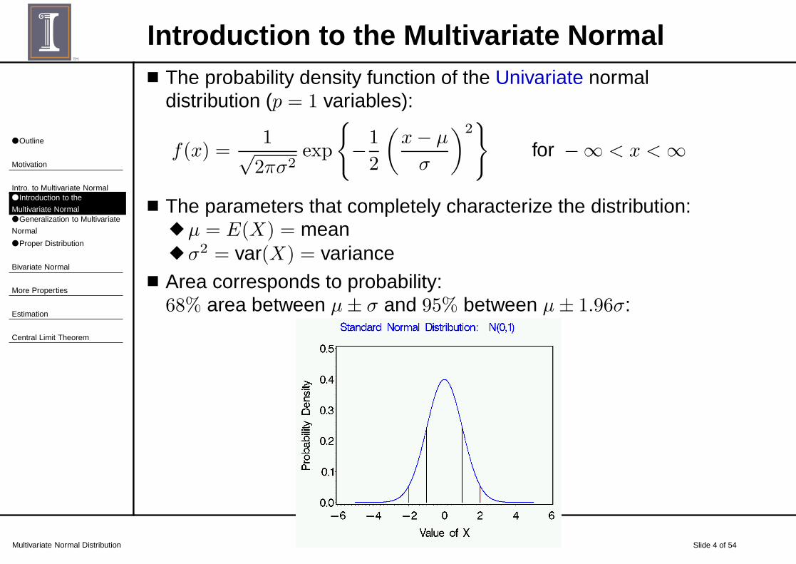
Introduction to the Multivariate Normal■ The probability density function of the Univariate normal

distribution (p = 1 variables):

f(x) =1√2πσ2

exp

{

−1

2

(x− µ

σ

)2}

for −∞ < x < ∞

■ The parameters that completely characterize the distribution:◆ µ = E(X) = mean◆ σ2 = var(X) = variance

■ Area corresponds to probability:68% area between µ± σ and 95% between µ± 1.96σ:

● Outline

Motivation



Normal


Bivariate Normal

More Properties

Estimation



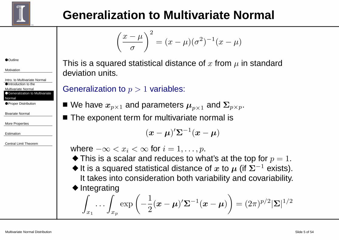
Generalization to Multivariate Normal(x− µ

σ

)2

= (x− µ)(σ2)−1(x− µ)

This is a squared statistical distance of x from µ in standarddeviation units.

Generalization to p > 1 variables:

■ We have xp×1 and parameters µp×1 and Σp×p.■ The exponent term for multivariate normal is

(x− µ)′Σ−1(x− µ)

where −∞ < xi < ∞ for i = 1, . . . , p.◆ This is a scalar and reduces to what’s at the top for p = 1.◆ It is a squared statistical distance of x to µ (if Σ−1 exists).

It takes into consideration both variability and covariability.◆ Integrating∫

x1

. . .

∫

xp

exp

(

−1

2(x− µ)′Σ−1(x− µ)

)

= (2π)p/2|Σ|1/2

● Outline

Motivation



Normal


Bivariate Normal

More Properties

Estimation



Proper DistributionSince the sum of probabilities over all possible values mustadd up to 1, we need to divide by (2π)p/2|Σ|1/2 to get a“proper” density function.

Multivariate Normal density function:

f(x) =1

(2π)p/2|Σ|1/2 exp

(

−1

2(x− µ)′Σ−1(x− µ)

)

where −∞ < xi < ∞ for i = 1, . . . , p.

To denote this, we use

Np(µ,Σ)

For p = 1, this reduces to the univariate normal p.d.f.

● Outline

Motivation


Bivariate Normal

● Bivariate Normal: p = 2● Bivariate Normal & Statistical

Distance● Bivariate Normal &

Independence

● Picture: µk = 0,

σkk = 1, r = 0.0

● Overhead µk = 0,

σkk = 1, r = 0.0


σkk = 1, r = 0.75

● Overhead: µk = 0,

σkk = 1, r = 0.75

● Summary: Comparing

r = 0.0 vs r = 0.75

● Real Time Software Demo● Slices of Multivariate Normal

Density

● Example Probability Contours

● Eigenvectors & Values

● Probability Contours: Axes of

ellipsoid


ellipsoid

● Example: Axses of Ellipses &

Prob. Contours

● Major Axis

● Minor Axis

● Graph of 95% Probability


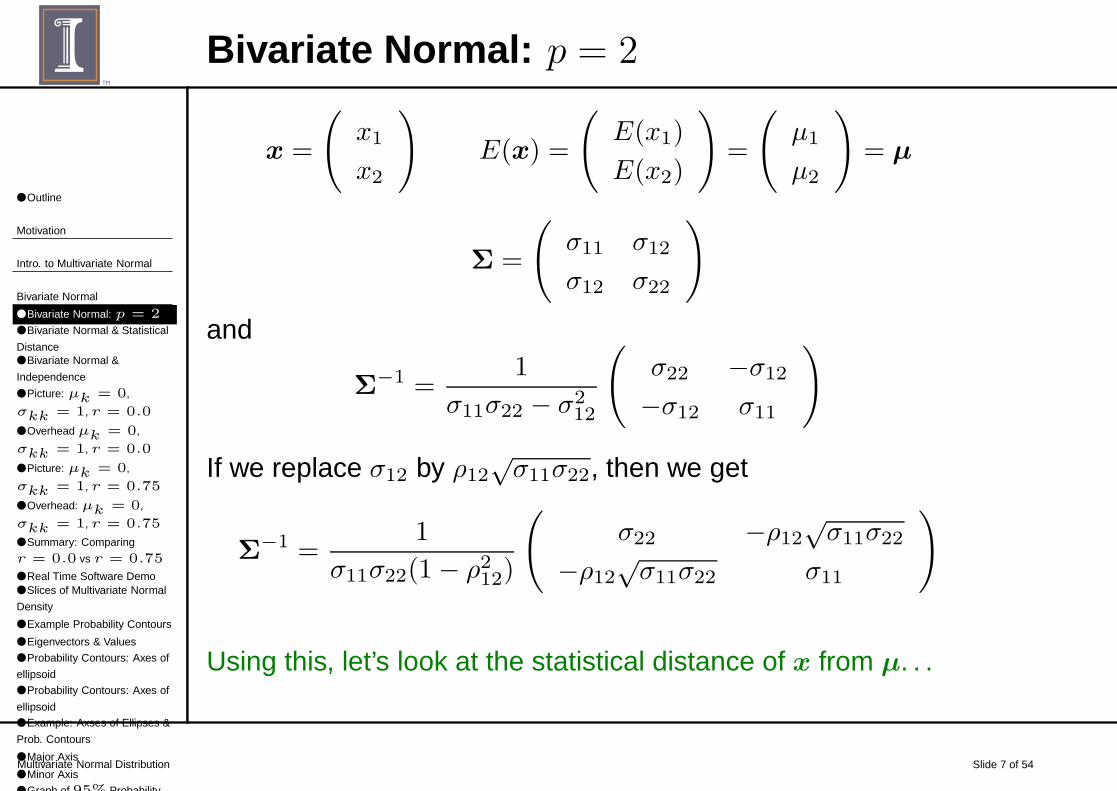
Bivariate Normal: p = 2

x =

(

x1

x2

)

E(x) =

(

E(x1)

E(x2)

)

=

(

µ1

µ2

)

= µ

Σ =

(

σ11 σ12

σ12 σ22

)

and

Σ−1 =

1

σ11σ22 − σ212

(

σ22 −σ12

−σ12 σ11

)

If we replace σ12 by ρ12√σ11σ22, then we get

Σ−1 =

1

σ11σ22(1− ρ212)

(

σ22 −ρ12√σ11σ22

−ρ12√σ11σ22 σ11

)

Using this, let’s look at the statistical distance of x from µ. . .

● Outline

Motivation


Bivariate Normal



Independence


σkk = 1, r = 0.0


σkk = 1, r = 0.0


σkk = 1, r = 0.75


σkk = 1, r = 0.75


r = 0.0 vs r = 0.75


Density




ellipsoid


ellipsoid


Prob. Contours

● Major Axis

● Minor Axis



Bivariate Normal & Statistical DistanceThe quantity in the exponent of the bivariate normal is

(x− µ)′Σ−1(x− µ)

= ((x1 − µ1), (x2 − µ2))

(1

σ11σ22(1− ρ212)

)

×(

σ22 −ρ12√σ11σ22

−ρ12√σ11σ22 σ11

)(

x1 − µ1

x2 − µ2

)

=1

1− ρ212

{(x1 − µ1√

σ11

)2

+

(x2 − µ2√

σ22

)2

− 2ρ12

(x1 − µ1√

σ11

)(x2 − µ2√

σ22

)}

=1

1− ρ212

{z21 + z22 − 2ρ12z1z2

}

● Outline

Motivation


Bivariate Normal



Independence


σkk = 1, r = 0.0


σkk = 1, r = 0.0


σkk = 1, r = 0.75


σkk = 1, r = 0.75


r = 0.0 vs r = 0.75


Density




ellipsoid


ellipsoid


Prob. Contours

● Major Axis

● Minor Axis



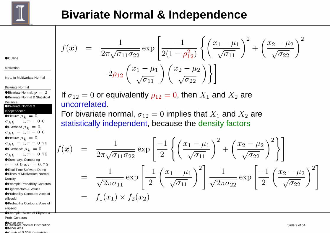
Bivariate Normal & Independence

f(x) =1

2π√σ11σ22

exp

[

−1

2(1− ρ212)

{(x1 − µ1√

σ11

)2

+

(x2 − µ2√

σ22

)2

−2ρ12

(x1 − µ1√

σ11

)(x2 − µ2√

σ22

)}]

If σ12 = 0 or equivalently ρ12 = 0, then X1 and X2 areuncorrelated.For bivariate normal, σ12 = 0 implies that X1 and X2 arestatistically independent, because the density factors

f(x) =1

2π√σ11σ22

exp

[

−1

2

{(x1 − µ1√

σ11

)2

+

(x2 − µ2√

σ22

)2}]

=1√

2πσ11exp

[

−1

2

(x1 − µ1√

σ11

)2]

1√2πσ22

exp

[

−1

2

(x2 − µ2√

σ22

)2]

= f1(x1)× f2(x2)

● Outline

Motivation


Bivariate Normal



Independence


σkk = 1, r = 0.0


σkk = 1, r = 0.0


σkk = 1, r = 0.75


σkk = 1, r = 0.75


r = 0.0 vs r = 0.75


Density




ellipsoid


ellipsoid


Prob. Contours

● Major Axis

● Minor Axis



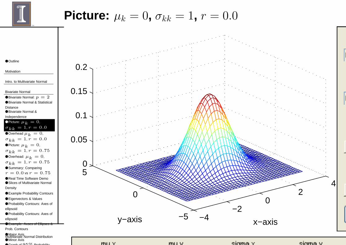
Picture: µk = 0, σkk = 1, r = 0.0

−4−2

02

4

−5

0

50

0.05

0.1

0.15

0.2

x−axisy−axis

● Outline

Motivation


Bivariate Normal



Independence


σkk = 1, r = 0.0


σkk = 1, r = 0.0


σkk = 1, r = 0.75


σkk = 1, r = 0.75


r = 0.0 vs r = 0.75


Density




ellipsoid


ellipsoid


Prob. Contours

● Major Axis

● Minor Axis



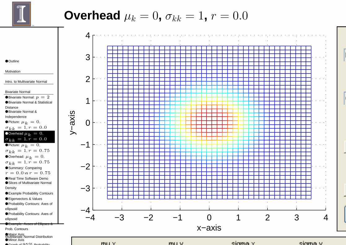
Overhead µk = 0, σkk = 1, r = 0.0

−4 −3 −2 −1 0 1 2 3 4−4

−3

−2

−1

0

1

2

3

4

x−axis

y−ax

is

● Outline

Motivation


Bivariate Normal



Independence


σkk = 1, r = 0.0


σkk = 1, r = 0.0


σkk = 1, r = 0.75


σkk = 1, r = 0.75


r = 0.0 vs r = 0.75


Density




ellipsoid


ellipsoid


Prob. Contours

● Major Axis

● Minor Axis



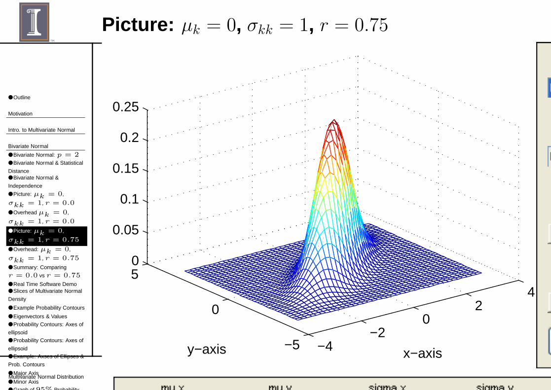
Picture: µk = 0, σkk = 1, r = 0.75

−4−2

02

4

−5

0

50

0.05

0.1

0.15

0.2

0.25

x−axisy−axis

● Outline

Motivation


Bivariate Normal



Independence


σkk = 1, r = 0.0


σkk = 1, r = 0.0


σkk = 1, r = 0.75


σkk = 1, r = 0.75


r = 0.0 vs r = 0.75


Density




ellipsoid


ellipsoid


Prob. Contours

● Major Axis

● Minor Axis



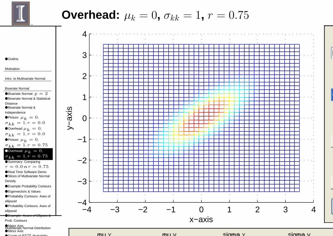
Overhead: µk = 0, σkk = 1, r = 0.75

−4 −3 −2 −1 0 1 2 3 4−4

−3

−2

−1

0

1

2

3

4

x−axis

y−ax

is

● Outline

Motivation


Bivariate Normal



Independence


σkk = 1, r = 0.0


σkk = 1, r = 0.0


σkk = 1, r = 0.75


σkk = 1, r = 0.75


r = 0.0 vs r = 0.75


Density




ellipsoid


ellipsoid


Prob. Contours

● Major Axis

● Minor Axis



Summary: Comparing r = 0.0 vs r = 0.75

For the figures shown, µ1 = µ2 = 0 and σ11 = σ22 = 1:

■ With r = 0.0,◆ Σ = diag(σ11, σ22), a diagonal matrix.◆ Density is “random” in the x-y plane.◆ When take a slice parallel to x-y, you get a circle.

■ When r = .75,◆ Σ is not a diagonal .◆ Density is not random in x-y plane.◆ There is a linear tilt (ie., density is concentrated on a line).◆ When you take a slice you get an ellipse that’s tilted.◆ Tilt depends on relative values of σ11 and σ22 (and scale

used in plotting).

■ When Σ = σ2I (i.e., diagonal with equal variances), it’s“spherical normal”.

● Outline

Motivation


Bivariate Normal



Independence


σkk = 1, r = 0.0


σkk = 1, r = 0.0


σkk = 1, r = 0.75


σkk = 1, r = 0.75


r = 0.0 vs r = 0.75


Density




ellipsoid


ellipsoid


Prob. Contours

● Major Axis

● Minor Axis



Real Time Software Demo

■ binormal.m (Peter Dunn)

■ Graph Bivariate .R(http://www.stat.ucl.ac.be/ISpersonnel/lecoutre/stats/fichiers/˜gallery.pdf)

● Outline

Motivation


Bivariate Normal



Independence


σkk = 1, r = 0.0


σkk = 1, r = 0.0


σkk = 1, r = 0.75


σkk = 1, r = 0.75


r = 0.0 vs r = 0.75


Density




ellipsoid


ellipsoid


Prob. Contours

● Major Axis

● Minor Axis



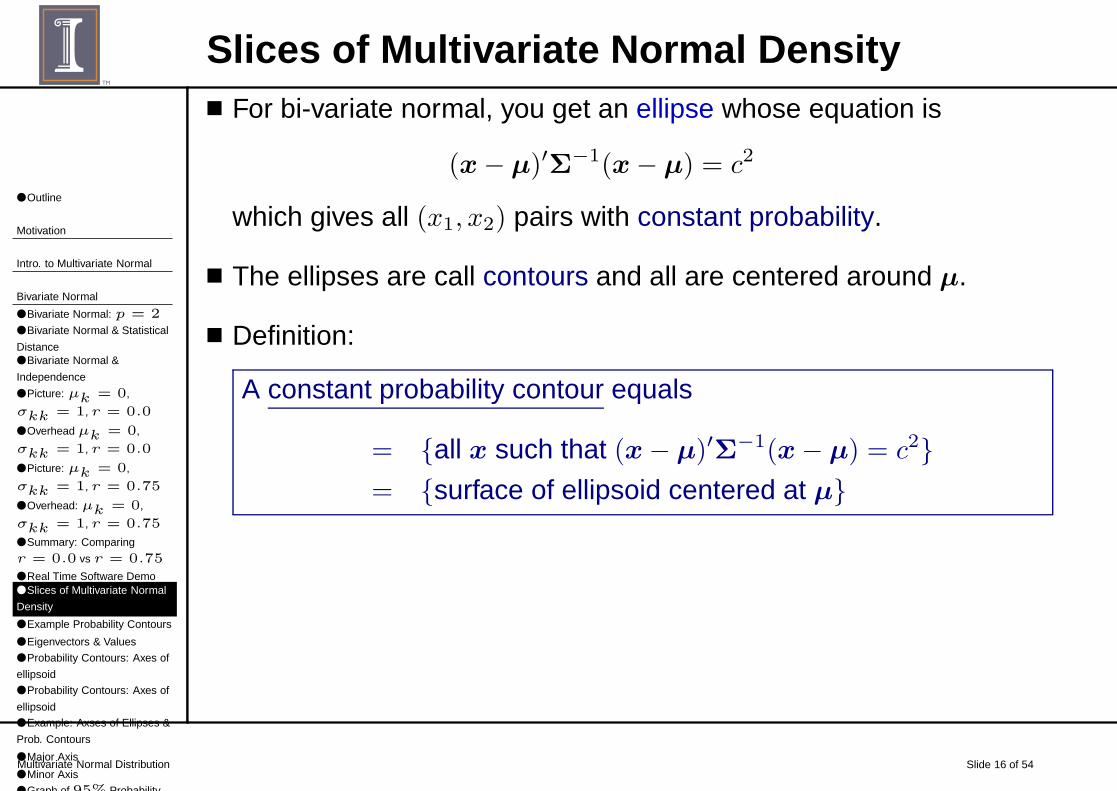
Slices of Multivariate Normal Density■ For bi-variate normal, you get an ellipse whose equation is

(x− µ)′Σ−1(x− µ) = c2

which gives all (x1, x2) pairs with constant probability.

■ The ellipses are call contours and all are centered around µ.

■ Definition:

A constant probability contour equals

= {all x such that (x− µ)′Σ−1(x− µ) = c2}= {surface of ellipsoid centered at µ}

● Outline

Motivation


Bivariate Normal



Independence


σkk = 1, r = 0.0


σkk = 1, r = 0.0


σkk = 1, r = 0.75


σkk = 1, r = 0.75


r = 0.0 vs r = 0.75


Density




ellipsoid


ellipsoid


Prob. Contours

● Major Axis

● Minor Axis



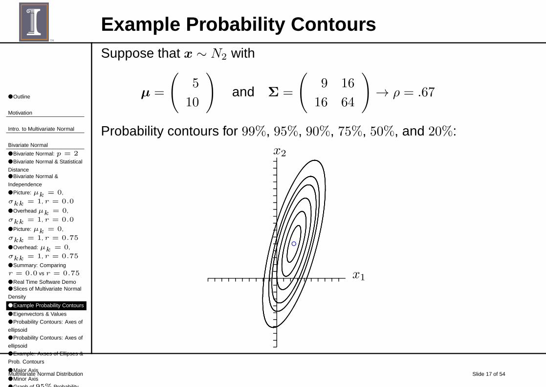
Example Probability ContoursSuppose that x ∼ N2 with

µ =

(

5

10

)

and Σ =

(

9 16

16 64

)

→ ρ = .67

Probability contours for 99%, 95%, 90%, 75%, 50%, and 20%:

x1

x2

b

● Outline

Motivation


Bivariate Normal



Independence


σkk = 1, r = 0.0


σkk = 1, r = 0.0


σkk = 1, r = 0.75


σkk = 1, r = 0.75


r = 0.0 vs r = 0.75


Density




ellipsoid


ellipsoid


Prob. Contours

● Major Axis

● Minor Axis



Eigenvectors & Values

To get the axes of the ellipsoids of probability contours. . . a littlemore on eigenvectors and eigenvalues . . .

■ Recall that eigenvectors ei and eigenvalues λi are solutionsto

Σei = λiei i = 1, 2, . . . p

where Σp×p symmetric and ei is a (p× 1) vector.

■ If Σ is positive definite (so that Σ−1 exists), then

Σe = λe implies Σ−1e =

(1

λ

)

e

● Outline

Motivation


Bivariate Normal



Independence


σkk = 1, r = 0.0


σkk = 1, r = 0.0


σkk = 1, r = 0.75


σkk = 1, r = 0.75


r = 0.0 vs r = 0.75


Density




ellipsoid


ellipsoid


Prob. Contours

● Major Axis

● Minor Axis



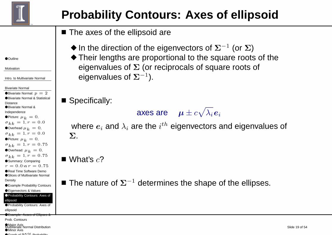
Probability Contours: Axes of ellipsoid■ The axes of the ellipsoid are

◆ In the direction of the eigenvectors of Σ−1 (or Σ)◆ Their lengths are proportional to the square roots of the

eigenvalues of Σ (or reciprocals of square roots ofeigenvalues of Σ−1).

■ Specifically:

axes are µ± c√

λiei

where ei and λi are the ith eigenvectors and eigenvalues ofΣ.

■ What’s c?

■ The nature of Σ−1 determines the shape of the ellipses.

● Outline

Motivation


Bivariate Normal



Independence


σkk = 1, r = 0.0


σkk = 1, r = 0.0


σkk = 1, r = 0.75


σkk = 1, r = 0.75


r = 0.0 vs r = 0.75


Density




ellipsoid


ellipsoid


Prob. Contours

● Major Axis

● Minor Axis



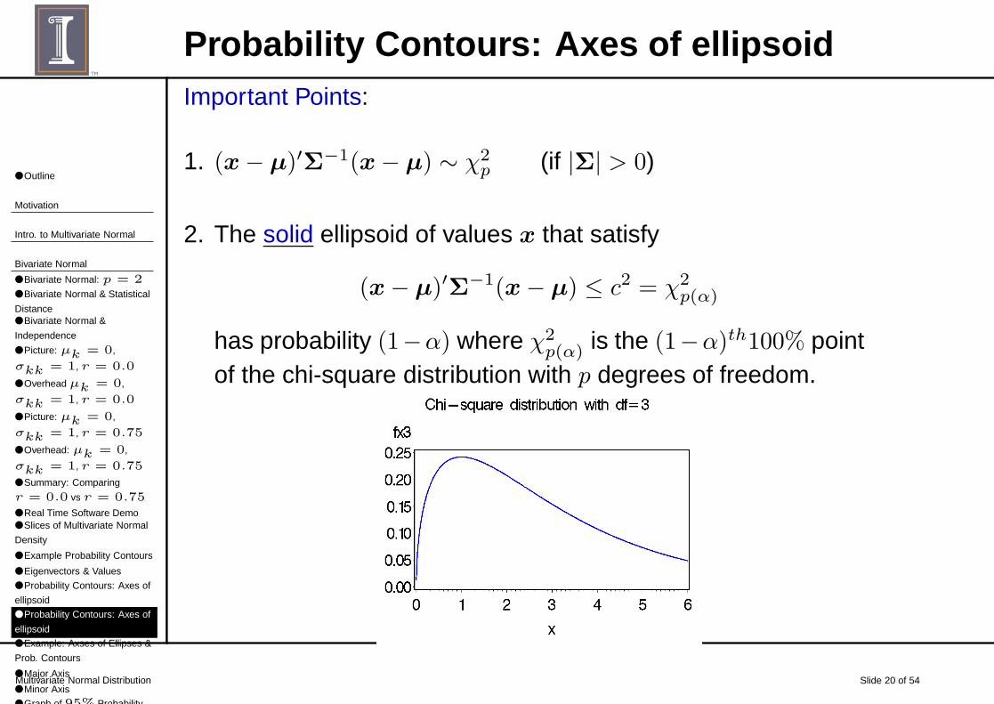
Probability Contours: Axes of ellipsoidImportant Points:

1. (x− µ)′Σ−1(x− µ) ∼ χ2p (if |Σ| > 0)

2. The solid ellipsoid of values x that satisfy

(x− µ)′Σ−1(x− µ) ≤ c2 = χ2p(α)

has probability (1−α) where χ2p(α) is the (1−α)th100% point

of the chi-square distribution with p degrees of freedom.

● Outline

Motivation


Bivariate Normal



Independence


σkk = 1, r = 0.0


σkk = 1, r = 0.0


σkk = 1, r = 0.75


σkk = 1, r = 0.75


r = 0.0 vs r = 0.75


Density




ellipsoid


ellipsoid


Prob. Contours

● Major Axis

● Minor Axis



Example: Axses of Ellipses & Prob. ContoursBack to the example where x ∼ N2 with

µ =

(

5

10

)

and Σ =

(

9 16

16 64

)

→ ρ = .667

and we want the “95% probability contour”.

The upper 5% point of the chi-square distribution with 2degrees of freedom is χ2

2(.05) = 5.9915, so

c =√5.9915 = 2.4478

Axes: µ± c√λiei where (λi, ei) is the ith (i = 1, 2)

eigenvalue/eigenvector pair of Σ.

λ1 = 68.316 e′1 = (.2604, .9655)

λ2 = 4.684 e′2 = (.9655,−.2604)

● Outline

Motivation


Bivariate Normal



Independence


σkk = 1, r = 0.0


σkk = 1, r = 0.0


σkk = 1, r = 0.75


σkk = 1, r = 0.75


r = 0.0 vs r = 0.75


Density




ellipsoid


ellipsoid


Prob. Contours

● Major Axis

● Minor Axis



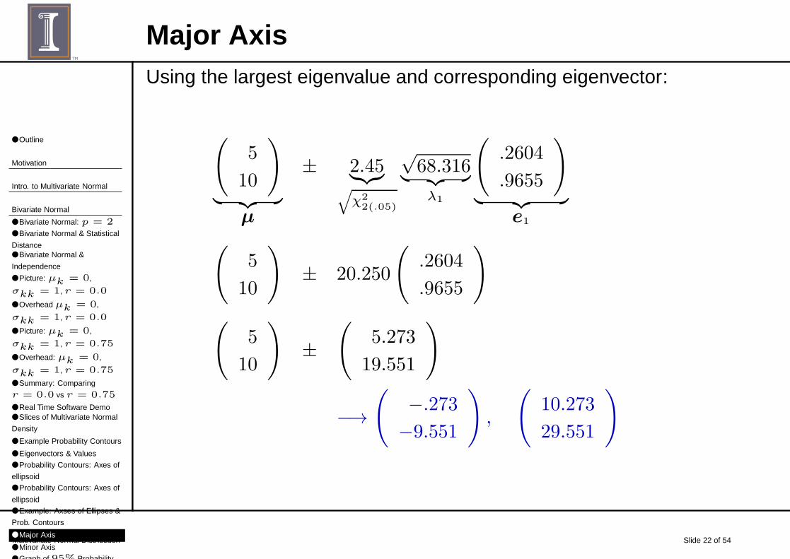
Major AxisUsing the largest eigenvalue and corresponding eigenvector:

(

5

10

)

︸︷︷︸

µ

± 2.45︸︷︷︸

√

χ22(.05)

√68.316

︸︷︷︸

λ1

(

.2604

.9655

)

︸︷︷︸

e1

(

5

10

)

± 20.250

(

.2604

.9655

)

(

5

10

)

±(

5.273

19.551

)

−→(

−.273

−9.551

)

,

(

10.273

29.551

)

● Outline

Motivation


Bivariate Normal



Independence


σkk = 1, r = 0.0


σkk = 1, r = 0.0


σkk = 1, r = 0.75


σkk = 1, r = 0.75


r = 0.0 vs r = 0.75


Density




ellipsoid


ellipsoid


Prob. Contours

● Major Axis

● Minor Axis



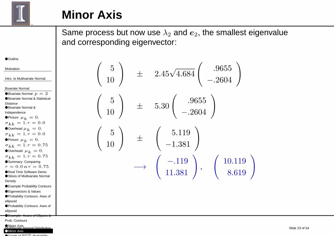
Minor AxisSame process but now use λ2 and e2, the smallest eigenvalueand corresponding eigenvector:

(

5

10

)

± 2.45√4.684

(

.9655

−.2604

)

(

5

10

)

± 5.30

(

.9655

−.2604

)

(

5

10

)

±(

5.119

−1.381

)

−→(

−.119

11.381

)

,

(

10.119

8.619

)

● Outline

Motivation


Bivariate Normal



Independence


σkk = 1, r = 0.0


σkk = 1, r = 0.0


σkk = 1, r = 0.75


σkk = 1, r = 0.75


r = 0.0 vs r = 0.75


Density




ellipsoid


ellipsoid


Prob. Contours

● Major Axis

● Minor Axis



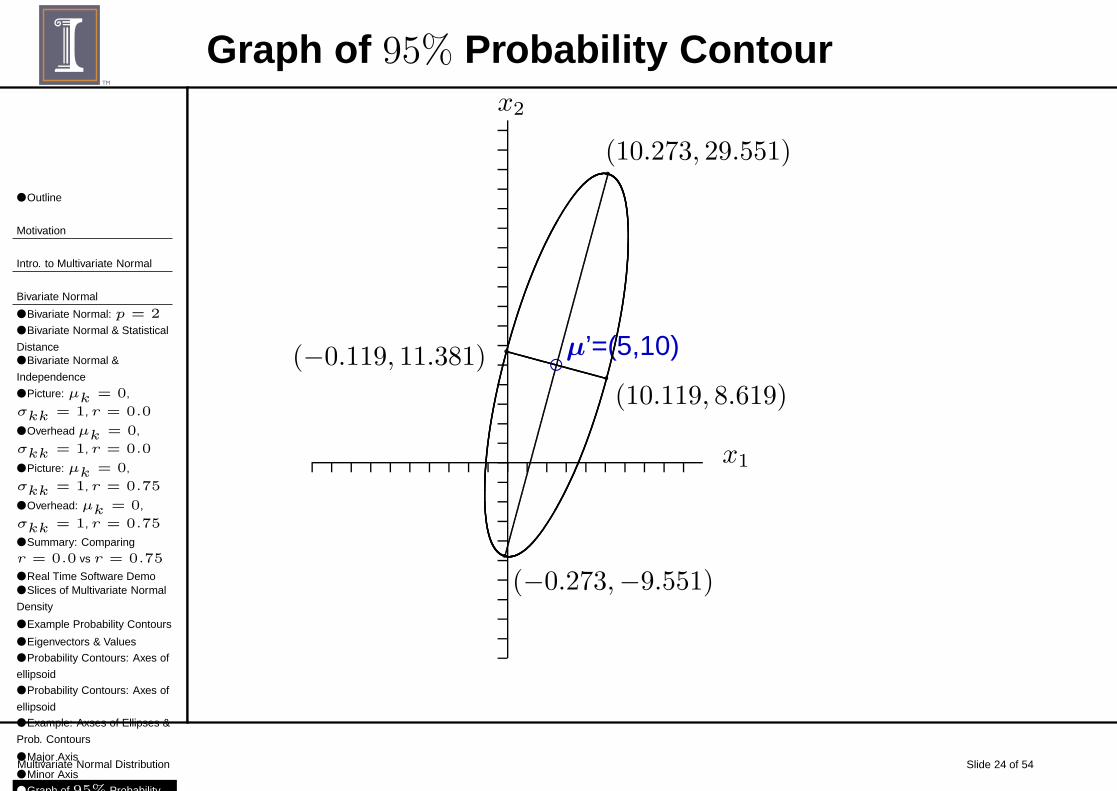
Graph of 95% Probability Contour

x1

x2

cµ’=(5,10)

`

(−0.273,−9.551)

`(10.273, 29.551)

`(−0.119, 11.381)`

(10.119, 8.619)

● Outline

Motivation


Bivariate Normal



Independence


σkk = 1, r = 0.0


σkk = 1, r = 0.0


σkk = 1, r = 0.75


σkk = 1, r = 0.75


r = 0.0 vs r = 0.75


Density




ellipsoid


ellipsoid


Prob. Contours

● Major Axis

● Minor Axis



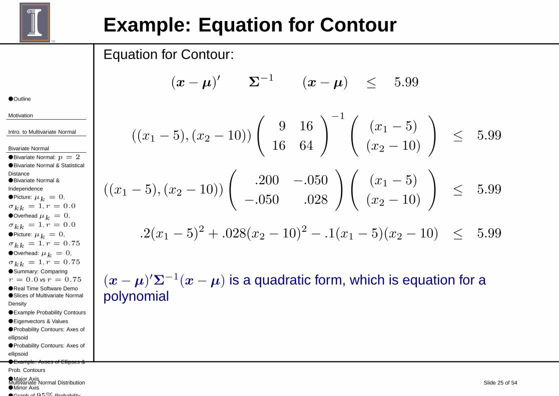
Example: Equation for ContourEquation for Contour:

(x− µ)′ Σ−1 (x− µ) ≤ 5.99

((x1 − 5), (x2 − 10))

(

9 16

16 64

)−1(

(x1 − 5)

(x2 − 10)

)

≤ 5.99

((x1 − 5), (x2 − 10))

(

.200 −.050

−.050 .028

)(

(x1 − 5)

(x2 − 10)

)

≤ 5.99

.2(x1 − 5)2 + .028(x2 − 10)2 − .1(x1 − 5)(x2 − 10) ≤ 5.99

(x− µ)′Σ−1(x− µ) is a quadratic form, which is equation for apolynomial

● Outline

Motivation


Bivariate Normal



Independence


σkk = 1, r = 0.0


σkk = 1, r = 0.0


σkk = 1, r = 0.75


σkk = 1, r = 0.75


r = 0.0 vs r = 0.75


Density




ellipsoid


ellipsoid


Prob. Contours

● Major Axis

● Minor Axis



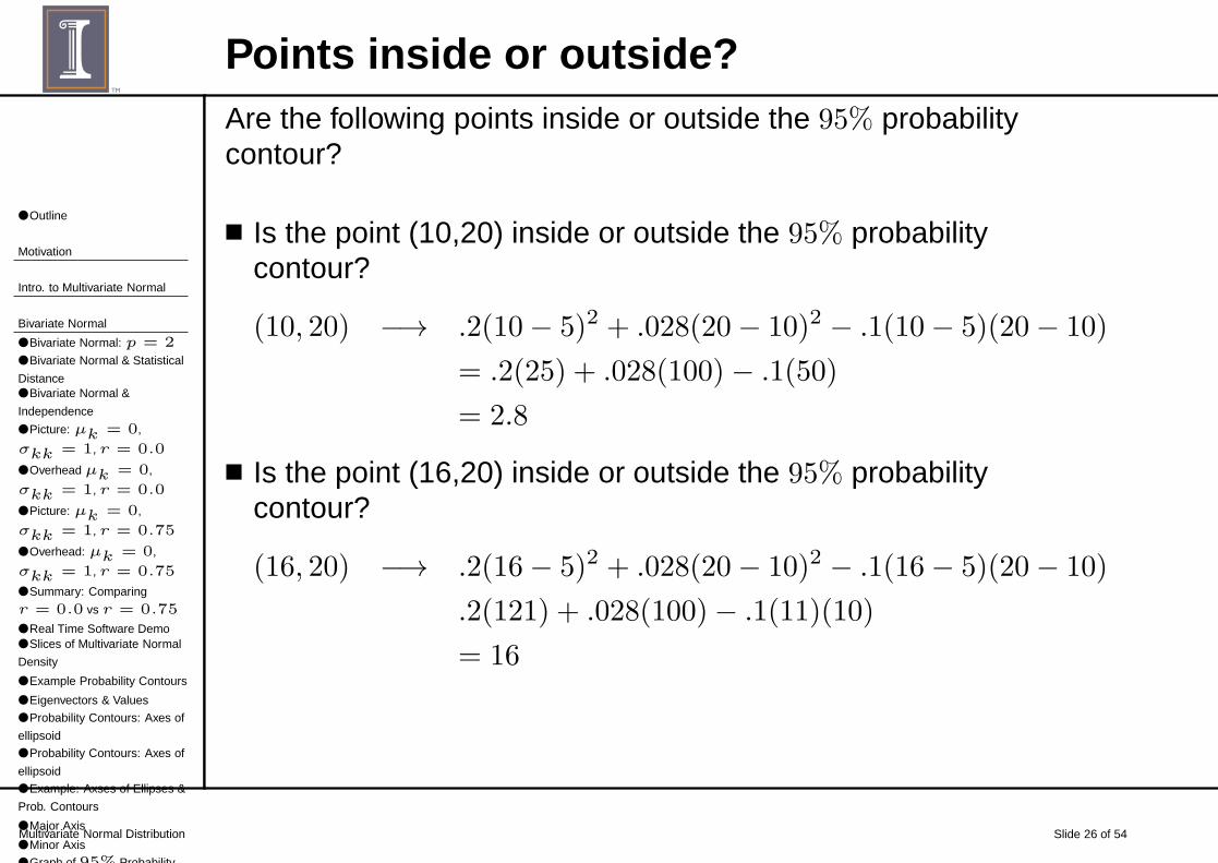
Points inside or outside?Are the following points inside or outside the 95% probabilitycontour?

■ Is the point (10,20) inside or outside the 95% probabilitycontour?

(10, 20) −→ .2(10− 5)2 + .028(20− 10)2 − .1(10− 5)(20− 10)

= .2(25) + .028(100)− .1(50)

= 2.8

■ Is the point (16,20) inside or outside the 95% probabilitycontour?

(16, 20) −→ .2(16− 5)2 + .028(20− 10)2 − .1(16− 5)(20− 10)

.2(121) + .028(100)− .1(11)(10)

= 16

● Outline

Motivation


Bivariate Normal



Independence


σkk = 1, r = 0.0


σkk = 1, r = 0.0


σkk = 1, r = 0.75


σkk = 1, r = 0.75


r = 0.0 vs r = 0.75


Density




ellipsoid


ellipsoid


Prob. Contours

● Major Axis

● Minor Axis



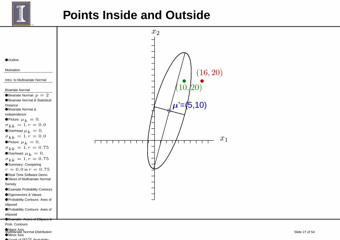
Points Inside and Outside

x1

x2

cµ’=(5,10)

s

(10, 20)s

(16, 20)

● Outline

Motivation


Bivariate Normal

More Properties● More Properties that we’ll

Expand on

● 1: Linear Combinations

● More Linear Combinations● Numerical Example with

Multiple Combinations● Multiple Regression as an

Example● Multiple Regression as an

Example

● Distribution of Y

● Least Square Estimation

● What’s the distribution of β?

● The distribution of Y

● The distribution of ǫ

● 2: Sub-sets of Variables● Sub-sets of Variables

continued

● Little Example on Sub-sets

● 3: Zero Covariance &

Statistical Independence

● Example

● 4: Conditional Distributions● Conditional Distribution for

q1 = q2 = 1

● Multiple Regression as a

Conditional Dist.


More Properties that we’ll Expand on

If X ∼ Np(µ,Σ), then

1. Linear combinations of components of X are (multivariate)normal.

2. All sub-sets of the components of X are (multivariate)normal.

3. Zero covariance implies that the corresponding componentsof X are statistical independent.

4. The conditional distributions of the components of X are(multivariate) normal.

● Outline

Motivation


Bivariate Normal


Expand on





Example







continued




● Example


q1 = q2 = 1


Conditional Dist.


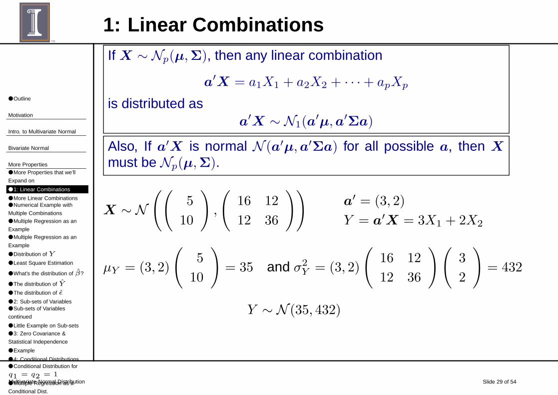
1: Linear CombinationsIf X ∼ Np(µ,Σ), then any linear combination

a′X = a1X1 + a2X2 + · · ·+ apXp

is distributed asa′X ∼ N1(a

′µ,a′Σa)

Also, If a′X is normal N (a′µ,a′Σa) for all possible a, then X

must be Np(µ,Σ).

X ∼ N((

5

10

)

,

(

16 12

12 36

))

a′ = (3, 2)

Y = a′X = 3X1 + 2X2

µY = (3, 2)

(

5

10

)

= 35 and σ2Y = (3, 2)

(

16 12

12 36

)(

3

2

)

= 432

Y ∼ N (35, 432)

● Outline

Motivation


Bivariate Normal


Expand on





Example







continued




● Example


q1 = q2 = 1


Conditional Dist.


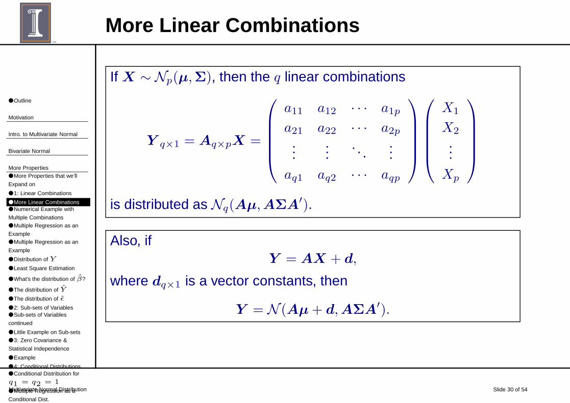
More Linear Combinations

If X ∼ Np(µ,Σ), then the q linear combinations

Y q×1 = Aq×pX =

a11 a12 · · · a1p

a21 a22 · · · a2p...

.... . .

...aq1 aq2 · · · aqp

X1

X2

...Xp

is distributed as Nq(Aµ,AΣA′).

Also, ifY = AX + d,

where dq×1 is a vector constants, then

Y = N (Aµ+ d,AΣA′).

● Outline

Motivation


Bivariate Normal


Expand on





Example







continued




● Example


q1 = q2 = 1


Conditional Dist.


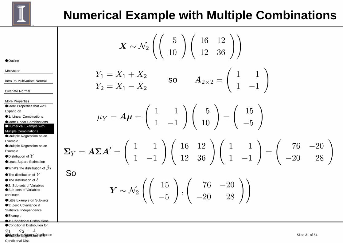
Numerical Example with Multiple Combinations

X ∼ N2

((

5

10

)(

16 12

12 36

))

Y1 = X1 +X2

Y2 = X1 −X2

so A2×2 =

(

1 1

1 −1

)

µY = Aµ =

(

1 1

1 −1

)(

5

10

)

=

(

15

−5

)

ΣY = AΣA′ =

(

1 1

1 −1

)(

16 12

12 36

)(

1 1

1 −1

)

=

(

76 −20

−20 28

)

So

Y ∼ N2

((

15

−5

)

,

(

76 −20

−20 28

))

● Outline

Motivation


Bivariate Normal


Expand on





Example







continued




● Example


q1 = q2 = 1


Conditional Dist.


Multiple Regression as an ExampleThis example will use what we know about linear combinationsand now what we know about the distribution of linearcombinations.

Linear Regression Model

■ Y = response variable.

■ Z1, Z2, . . . , Zr are predictor/explanatory variables, which areconsidered to be fixed.

■ The model is

Y = βo + β1Z1 + β2Z2 + . . .+ βrZr + ǫ

■ The error of prediction ǫ is viewed as a random variable.

● Outline

Motivation


Bivariate Normal


Expand on





Example







continued




● Example


q1 = q2 = 1


Conditional Dist.


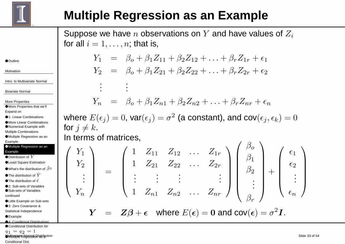
Multiple Regression as an ExampleSuppose we have n observations on Y and have values of Zi

for all i = 1, . . . , n; that is,

Y1 = βo + β1Z11 + β2Z12 + . . .+ βrZ1r + ǫ1

Y2 = βo + β1Z21 + β2Z22 + . . .+ βrZ2r + ǫ2...

...

Yn = βo + β1Zn1 + β2Zn2 + . . .+ βrZnr + ǫn

where E(ǫj) = 0, var(ǫj) = σ2 (a constant), and cov(ǫj , ǫk) = 0for j 6= k.In terms of matrices,

Y1

Y2

...Yn

=

1 Z11 Z12 . . . Z1r

1 Z21 Z22 . . . Z2r

......

......

1 Zn1 Zn2 . . . Znr

βo

β1

β2

...βr

+

ǫ1

ǫ2...

ǫn

Y = Zβ + ǫ where E(ǫ) = 0 and cov(ǫ) = σ2I.

● Outline

Motivation


Bivariate Normal


Expand on





Example







continued




● Example


q1 = q2 = 1


Conditional Dist.


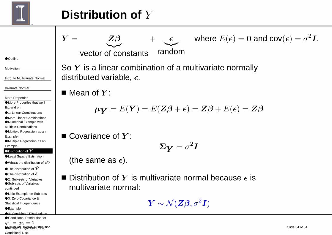
Distribution of Y

Y = Zβ︸︷︷︸

vector of constants

+ ǫ︸︷︷︸

random

where E(ǫ) = 0 and cov(ǫ) = σ2I.

So Y is a linear combination of a multivariate normallydistributed variable, ǫ.

■ Mean of Y :

µY = E(Y ) = E(Zβ + ǫ) = Zβ + E(ǫ) = Zβ

■ Covariance of Y :ΣY = σ2I

(the same as ǫ).

■ Distribution of Y is multivariate normal because ǫ ismultivariate normal:

Y ∼ N (Zβ, σ2I)

● Outline

Motivation


Bivariate Normal


Expand on





Example







continued




● Example


q1 = q2 = 1


Conditional Dist.


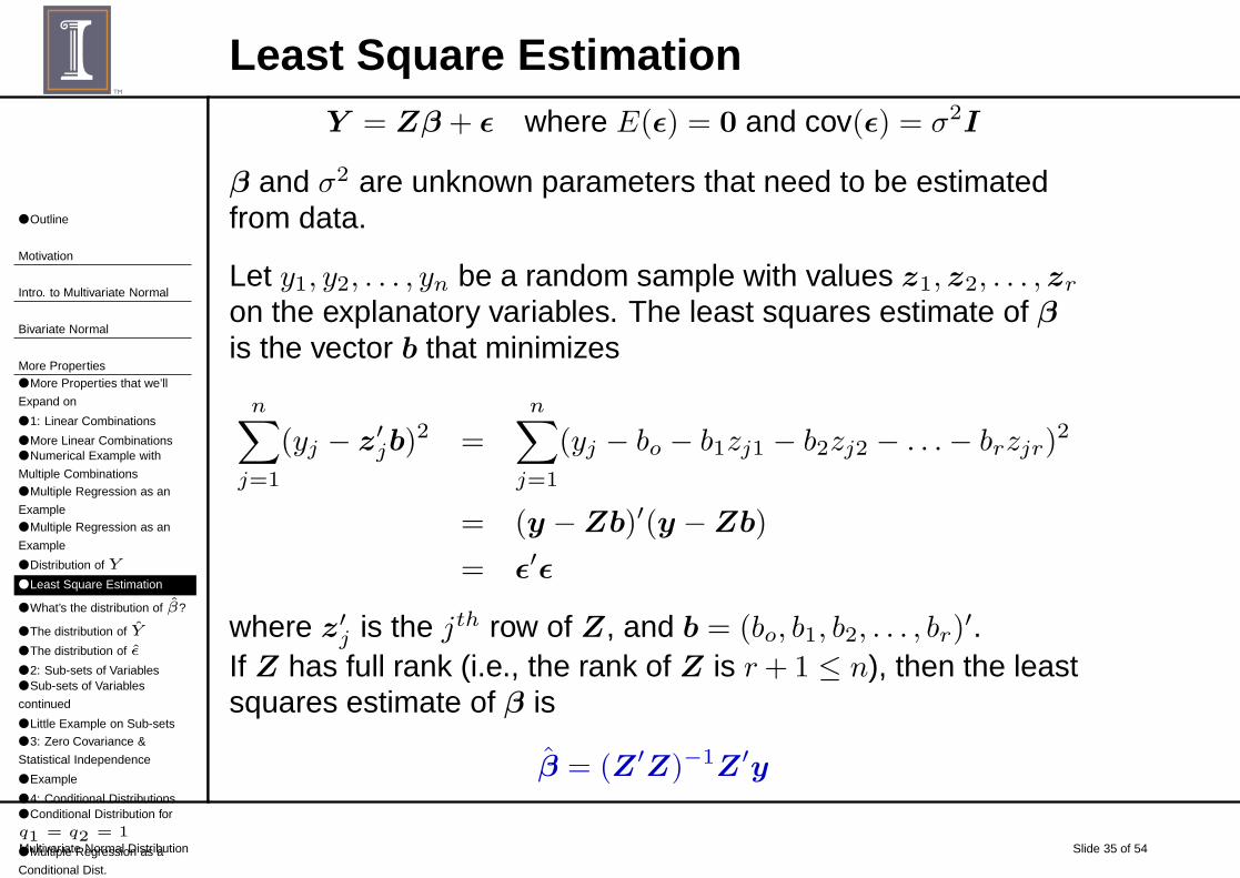
Least Square EstimationY = Zβ + ǫ where E(ǫ) = 0 and cov(ǫ) = σ2I

β and σ2 are unknown parameters that need to be estimatedfrom data.

Let y1, y2, . . . , yn be a random sample with values z1, z2, . . . , zr

on the explanatory variables. The least squares estimate of βis the vector b that minimizes

n∑

j=1

(yj − z′

jb)2 =

n∑

j=1

(yj − bo − b1zj1 − b2zj2 − . . .− brzjr)2

= (y −Zb)′(y −Zb)

= ǫ′ǫ

where z′

j is the jth row of Z, and b = (bo, b1, b2, . . . , br)′.

If Z has full rank (i.e., the rank of Z is r+ 1 ≤ n), then the leastsquares estimate of β is

β = (Z ′Z)−1Z ′y

● Outline

Motivation


Bivariate Normal


Expand on





Example







continued




● Example


q1 = q2 = 1


Conditional Dist.


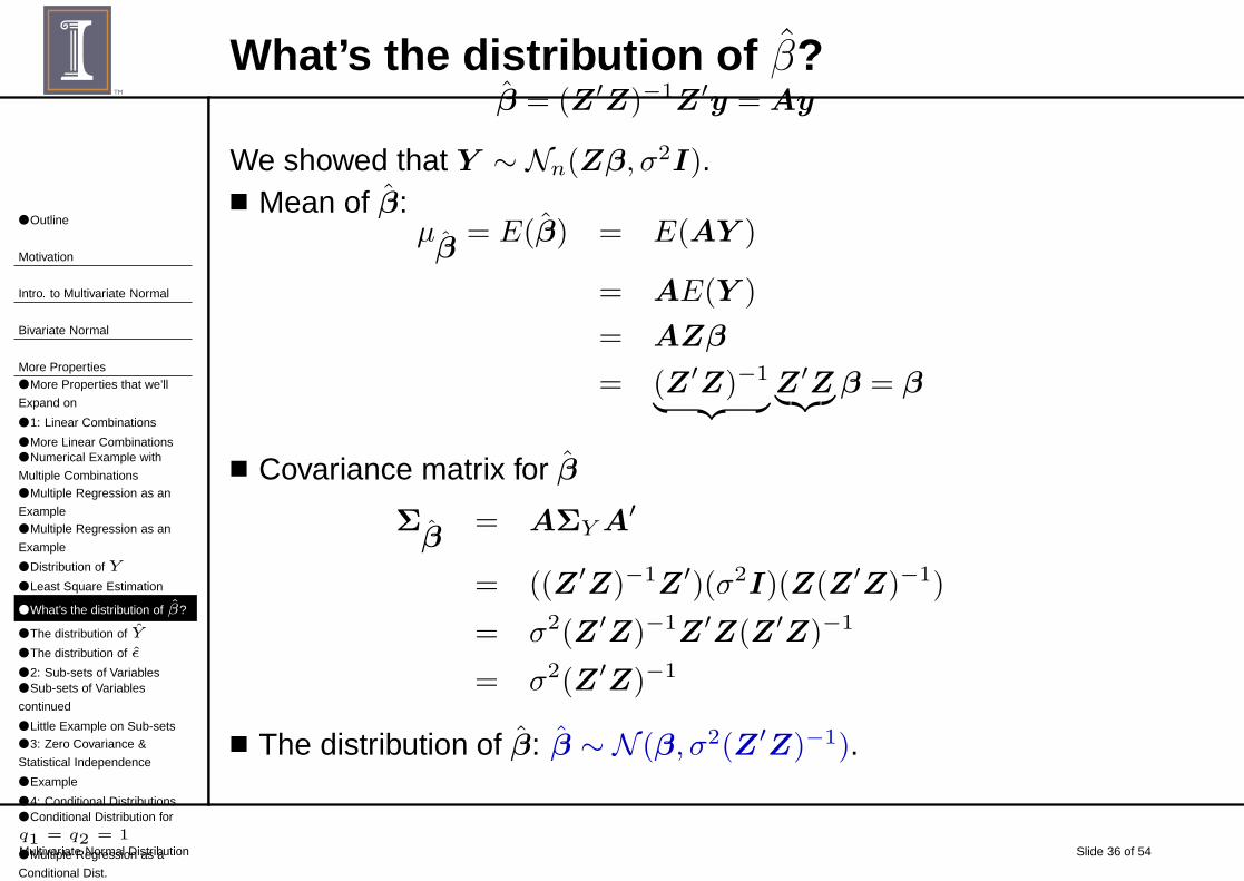
What’s the distribution of β?β = (Z ′Z)−1Z ′y = Ay

We showed that Y ∼ Nn(Zβ, σ2I).■ Mean of β:

µ ˆβ= E(β) = E(AY )

= AE(Y )

= AZβ

= (Z ′Z)−1

︸︷︷︸Z ′Z︸︷︷︸

β = β

■ Covariance matrix for β

Σ ˆβ= AΣY A

′

= ((Z ′Z)−1Z ′)(σ2I)(Z(Z ′Z)−1)

= σ2(Z ′Z)−1Z ′Z(Z ′Z)−1

= σ2(Z ′Z)−1

■ The distribution of β: β ∼ N (β, σ2(Z ′Z)−1).

● Outline

Motivation


Bivariate Normal


Expand on





Example







continued




● Example


q1 = q2 = 1


Conditional Dist.


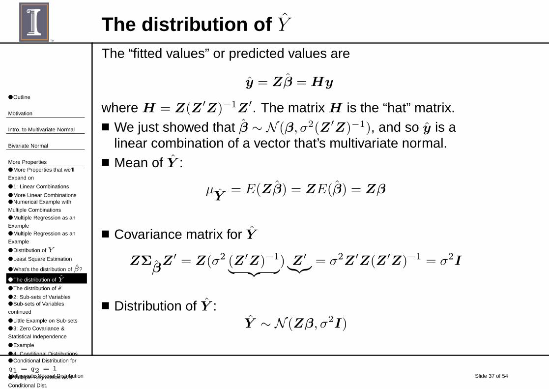
The distribution of YThe “fitted values” or predicted values are

y = Zβ = Hy

where H = Z(Z ′Z)−1Z ′. The matrix H is the “hat” matrix.■ We just showed that β ∼ N (β, σ2(Z ′Z)−1), and so y is a

linear combination of a vector that’s multivariate normal.■ Mean of Y :

µ ˆY= E(Zβ) = ZE(β) = Zβ

■ Covariance matrix for Y

ZΣ ˆβZ ′ = Z(σ2 (Z ′Z)−1

︸︷︷︸) Z ′

︸︷︷︸= σ2Z ′Z(Z ′Z)−1 = σ2I

■ Distribution of Y :Y ∼ N (Zβ, σ2I)

● Outline

Motivation


Bivariate Normal


Expand on





Example







continued




● Example


q1 = q2 = 1


Conditional Dist.


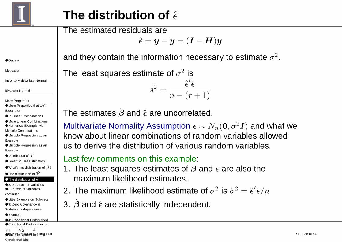
The distribution of ǫThe estimated residuals are

ǫ = y − y = (I −H)y

and they contain the information necessary to estimate σ2.

The least squares estimate of σ2 is

s2 =ǫ′ǫ

n− (r + 1)

The estimates β and ǫ are uncorrelated.

Multivariate Normality Assumption ǫ ∼ Nn(0, σ2I) and what we

know about linear combinations of random variables allowedus to derive the distribution of various random variables.

Last few comments on this example:1. The least squares estimates of β and ǫ are also the

maximum likelihood estimates.2. The maximum likelihood estimate of σ2 is σ2 = ǫ′ǫ/n

3. β and ǫ are statistically independent.

● Outline

Motivation


Bivariate Normal


Expand on





Example







continued




● Example


q1 = q2 = 1


Conditional Dist.


2: Sub-sets of Variables

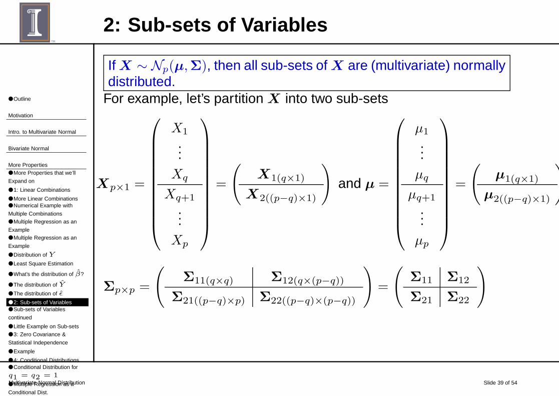
If X ∼ Np(µ,Σ), then all sub-sets of X are (multivariate) normallydistributed.

For example, let’s partition X into two sub-sets

Xp×1 =

X1

...Xq

Xq+1

...Xp

=

(

X1(q×1)

X2((p−q)×1)

)

and µ =

µ1

...µq

µq+1

...µp

=

(

µ1(q×1)

µ2((p−q)×1)

)

Σp×p =

(

Σ11(q×q) Σ12(q×(p−q))

Σ21((p−q)×p) Σ22((p−q)×(p−q))

)

=

(

Σ11 Σ12

Σ21 Σ22

)

● Outline

Motivation


Bivariate Normal


Expand on





Example







continued




● Example


q1 = q2 = 1


Conditional Dist.


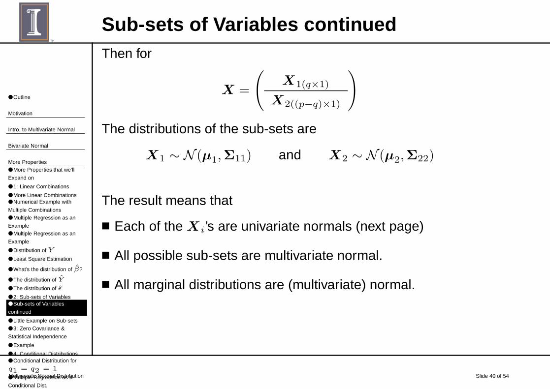
Sub-sets of Variables continuedThen for

X =

(

X1(q×1)

X2((p−q)×1)

)

The distributions of the sub-sets are

X1 ∼ N (µ1,Σ11) and X2 ∼ N (µ2,Σ22)

The result means that

■ Each of the Xi’s are univariate normals (next page)

■ All possible sub-sets are multivariate normal.

■ All marginal distributions are (multivariate) normal.

● Outline

Motivation


Bivariate Normal


Expand on





Example







continued




● Example


q1 = q2 = 1


Conditional Dist.


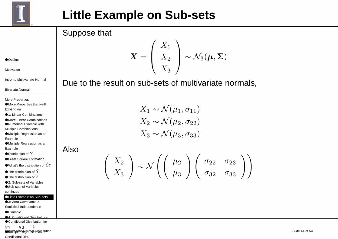
Little Example on Sub-setsSuppose that

X =

X1

X2

X3

∼ N3(µ,Σ)

Due to the result on sub-sets of multivariate normals,

X1 ∼ N (µ1, σ11)

X2 ∼ N (µ2, σ22)

X3 ∼ N (µ3, σ33)

Also (

X2

X3

)

∼ N((

µ2

µ3

)(

σ22 σ23

σ32 σ33

))

● Outline

Motivation


Bivariate Normal


Expand on





Example







continued




● Example


q1 = q2 = 1


Conditional Dist.


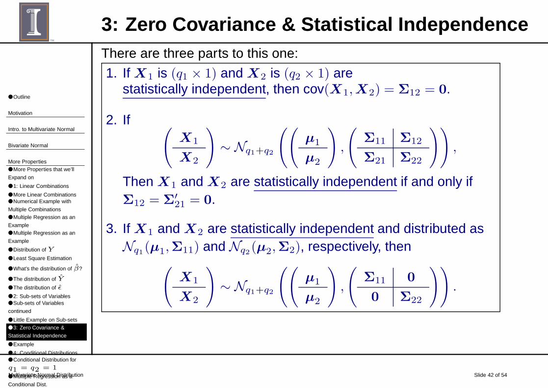
3: Zero Covariance & Statistical IndependenceThere are three parts to this one:

1. If X1 is (q1 × 1) and X2 is (q2 × 1) arestatistically independent, then cov(X1,X2) = Σ12 = 0.

2. If (

X1

X2

)

∼ Nq1+q2

((

µ1

µ2

)

,

(

Σ11 Σ12

Σ21 Σ22

))

,

Then X1 and X2 are statistically independent if and only ifΣ12 = Σ

′

21 = 0.

3. If X1 and X2 are statistically independent and distributed asNq1(µ1,Σ11) and Nq2(µ2,Σ2), respectively, then

(

X1

X2

)

∼ Nq1+q2

((

µ1

µ2

)

,

(

Σ11 0

0 Σ22

))

.

● Outline

Motivation


Bivariate Normal


Expand on





Example







continued




● Example


q1 = q2 = 1


Conditional Dist.


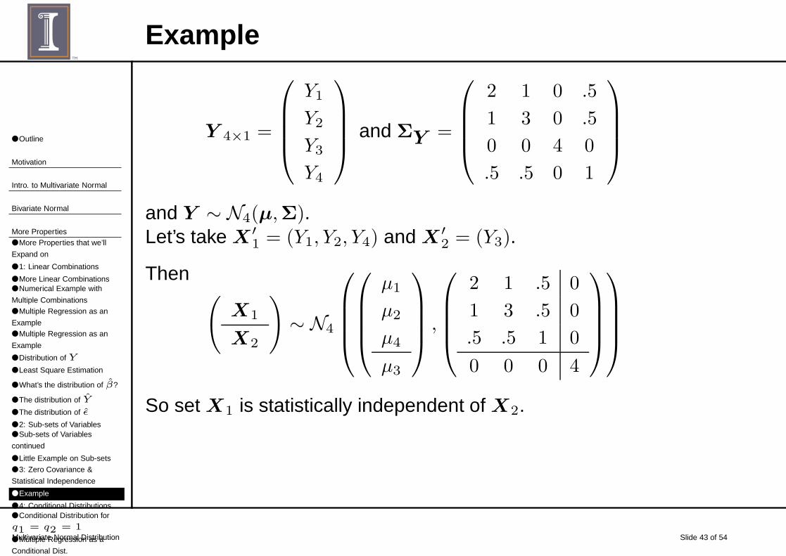
Example

Y 4×1 =

Y1

Y2

Y3

Y4

and ΣY =

2 1 0 .5

1 3 0 .5

0 0 4 0

.5 .5 0 1

and Y ∼ N4(µ,Σ).Let’s take X ′

1 = (Y1, Y2, Y4) and X ′

2 = (Y3).

Then(

X1

X2

)

∼ N4

µ1

µ2

µ4

µ3

,

2 1 .5 0

1 3 .5 0

.5 .5 1 0

0 0 0 4

So set X1 is statistically independent of X2.

● Outline

Motivation


Bivariate Normal


Expand on





Example







continued




● Example


q1 = q2 = 1


Conditional Dist.


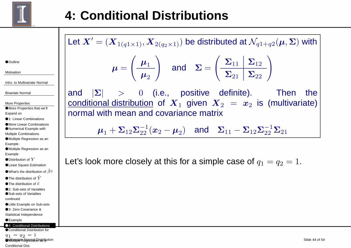
4: Conditional Distributions

Let X ′ = (X1(q1×1),X2(q2×1)) be distributed at Nq1+q2(µ,Σ) with

µ =

(

µ1

µ2

)

and Σ =

(

Σ11 Σ12

Σ21 Σ22

)

and |Σ| > 0 (i.e., positive definite). Then theconditional distribution of X1 given X2 = x2 is (multivariate)normal with mean and covariance matrix

µ1 +Σ12Σ−122 (x2 − µ2) and Σ11 −Σ12Σ

−122 Σ21

Let’s look more closely at this for a simple case of q1 = q2 = 1.

● Outline

Motivation


Bivariate Normal


Expand on





Example







continued




● Example


q1 = q2 = 1


Conditional Dist.


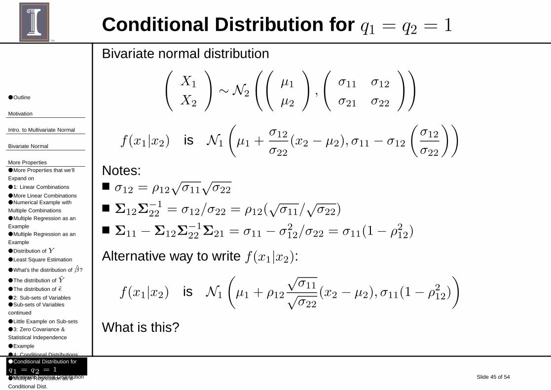
Conditional Distribution for q1 = q2 = 1

Bivariate normal distribution(

X1

X2

)

∼ N2

((

µ1

µ2

)

,

(

σ11 σ12

σ21 σ22

))

f(x1|x2) is N1

(

µ1 +σ12

σ22(x2 − µ2), σ11 − σ12

(σ12

σ22

))

Notes:■ σ12 = ρ12

√σ11

√σ22

■ Σ12Σ−122 = σ12/σ22 = ρ12(

√σ11/

√σ22)

■ Σ11 −Σ12Σ−122 Σ21 = σ11 − σ2

12/σ22 = σ11(1− ρ212)

Alternative way to write f(x1|x2):

f(x1|x2) is N1

(

µ1 + ρ12

√σ11√σ22

(x2 − µ2), σ11(1− ρ212)

)

What is this?

● Outline

Motivation


Bivariate Normal


Expand on





Example







continued




● Example


q1 = q2 = 1


Conditional Dist.


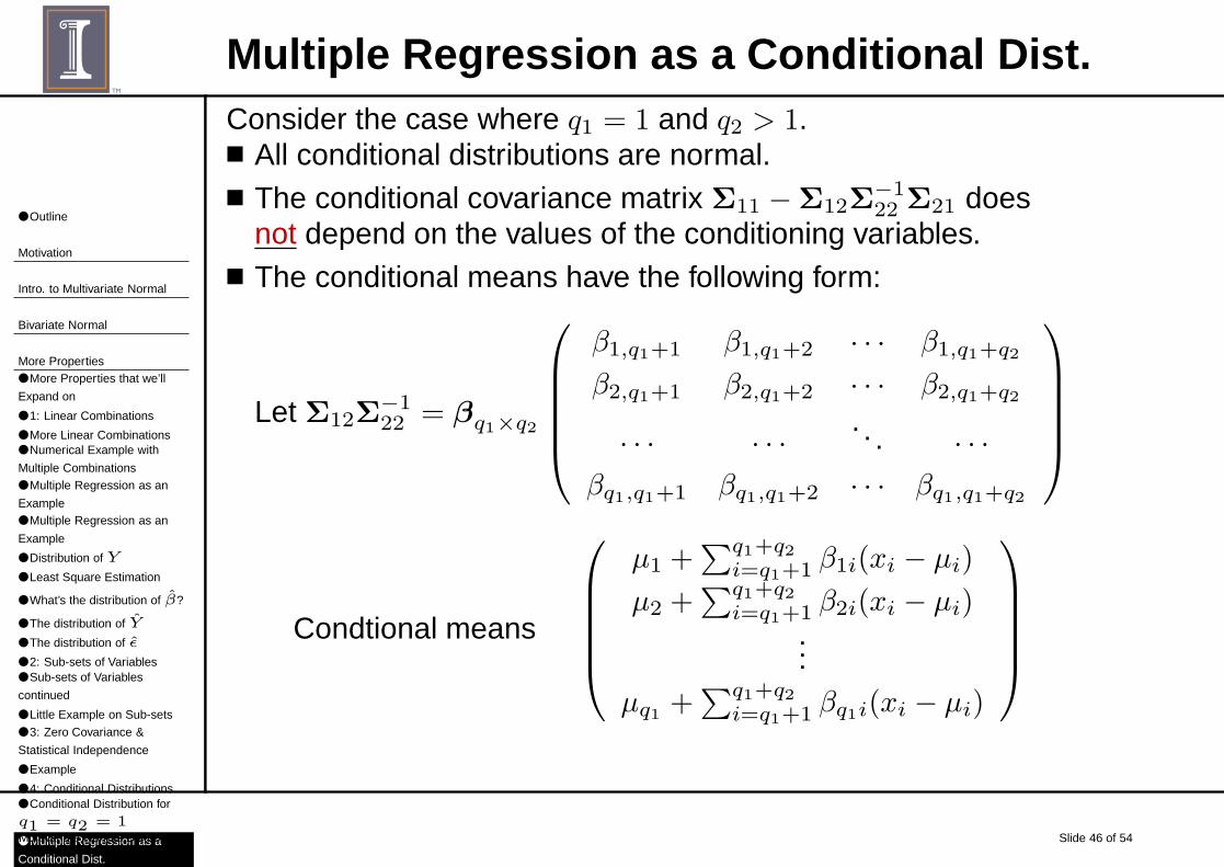
Multiple Regression as a Conditional Dist.Consider the case where q1 = 1 and q2 > 1.■ All conditional distributions are normal.■ The conditional covariance matrix Σ11 −Σ12Σ

−122 Σ21 does

not depend on the values of the conditioning variables.■ The conditional means have the following form:

Let Σ12Σ−122 = βq1×q2

β1,q1+1 β1,q1+2 · · · β1,q1+q2

β2,q1+1 β2,q1+2 · · · β2,q1+q2

· · · · · · . . . · · ·βq1,q1+1 βq1,q1+2 · · · βq1,q1+q2

Condtional means

µ1 +∑q1+q2

i=q1+1 β1i(xi − µi)

µ2 +∑q1+q2

i=q1+1 β2i(xi − µi)...

µq1 +∑q1+q2

i=q1+1 βq1i(xi − µi)

● Outline

Motivation


Bivariate Normal

More Properties

Estimation

● Estimation of µ and Σ

● Estimation of µ and Σ:

Multivariate Case

● Sampling Distribution of Σ



Estimation of µ and Σ

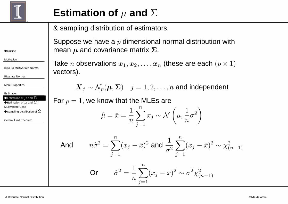
& sampling distribution of estimators.

Suppose we have a p dimensional normal distribution withmean µ and covariance matrix Σ.

Take n observations x1,x2, . . . ,xn (these are each (p× 1)vectors).

Xj ∼ Np(µ,Σ) j = 1, 2, . . . , n and independent

For p = 1, we know that the MLEs are

µ = x =1

n

n∑

j=1

xj ∼ N(

µ,1

nσ2

)

And nσ2 =n∑

j=1

(xj − x)2 and1

σ2

n∑

j=1

(xj − x)2 ∼ χ2(n−1)

Or σ2 =1

n

n∑

j=1

(xj − x)2 ∼ σ2χ2(n−1)

● Outline

Motivation


Bivariate Normal

More Properties

Estimation



Multivariate Case




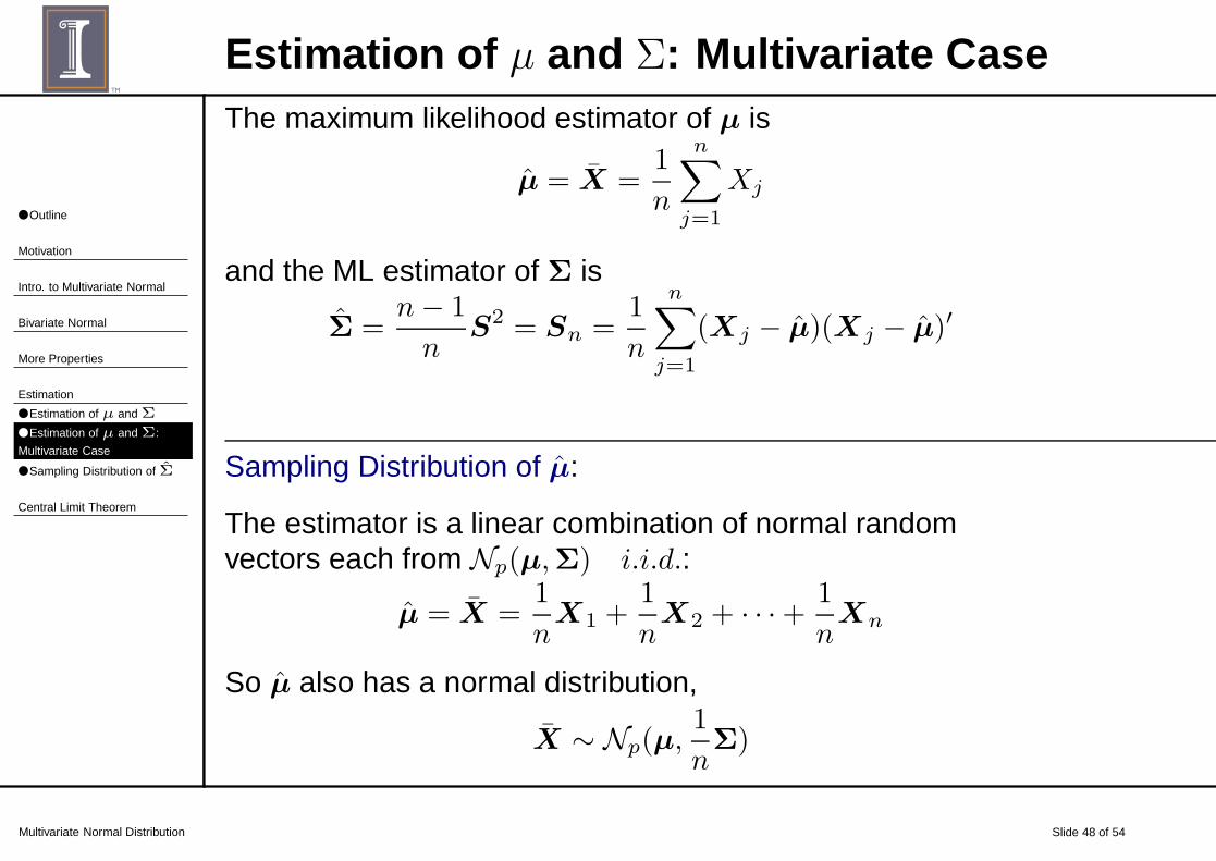
Estimation of µ and Σ: Multivariate CaseThe maximum likelihood estimator of µ is

µ = X =1

n

n∑

j=1

Xj

and the ML estimator of Σ is

Σ =n− 1

nS2 = Sn =

1

n

n∑

j=1

(Xj − µ)(Xj − µ)′

Sampling Distribution of µ:

The estimator is a linear combination of normal randomvectors each from Np(µ,Σ) i.i.d.:

µ = X =1

nX1 +

1

nX2 + · · ·+ 1

nXn

So µ also has a normal distribution,

X ∼ Np(µ,1

nΣ)

● Outline

Motivation


Bivariate Normal

More Properties

Estimation



Multivariate Case




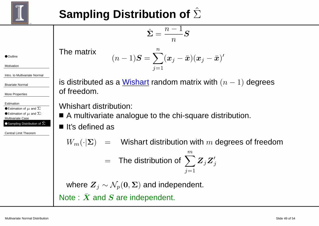
Sampling Distribution of Σ

Σ =n− 1

nS

The matrix(n− 1)S =

n∑

j=1

(xj − x)(xj − x)′

is distributed as a Wishart random matrix with (n− 1) degreesof freedom.

Whishart distribution:■ A multivariate analogue to the chi-square distribution.■ It’s defined as

Wm(·|Σ) = Wishart distribution with m degrees of freedom

= The distribution ofm∑

j=1

ZjZ′

j

where Zj ∼ Np(0,Σ) and independent.

Note : X and S are independent.

● Outline

Motivation


Bivariate Normal

More Properties

Estimation


● Law of Large Numbers

● Central Limit Theorem

● Few more comments● Comparison of Probability

Contours● Why So Much a Difference

with Only 20?


Law of Large NumbersData are not always (multivariate) normal

The Law of Large Numbers (for multivariate data):

Let X1,X2, . . . ,Xn be independent observations from apopulation with mean E(X) = µ.

Then X = (1/n)∑n

j=1 Xj converges in probability to µ as n

gets large; that is,

X → µ for large samples

AndS(or Sn) approach Σ for large samples

These are true regardless of the true distribution of the Xj ’s.

● Outline

Motivation


Bivariate Normal

More Properties

Estimation






with Only 20?


Central Limit TheoremLet Y 1,Y 2, . . . ,Y n be independent observations from apopulation with mean E(Y ) = µ and finite (non-singular, fullrank), covariance matrix Σ.

Then√n(X − µ) has an approximate N (0,Σ) distribution if

n >> p (i.e., “much larger than”).

So, for “large” n

X = Sample mean vector ≈ N (µ,1

nΣ),

regardless of the underlying distribution of the Y j ’s.

What if Σ is unknown? If n is large “enough”, S will be close toΣ, so

√n(X − µ) ≈ Np(0,S) or X ≈ Np(µ,

1

nS).

Since n(X − µ)′Σ−1(X − µ) ∼ χ2p,

n(X − µ)′S−1(X − µ) ≈ χ2p

● Outline

Motivation


Bivariate Normal

More Properties

Estimation






with Only 20?


Few more comments■ Using S instead of Σ does not seriously effect

approximation.

■ n must be large relative to p; that is, (n− p) is large.

■ The probability contours for X are tighter than those for Xsince we have (1/n)Σ for X rather than Σ for X.

See next slide for an example of the latter.

● Outline

Motivation


Bivariate Normal

More Properties

Estimation






with Only 20?


Comparison of Probability ContoursReturning to our example and pretending we have n = 20.Below are contours for 99%, 95%, 90%, 75%, 50% and 20%:

Contours for Xj

b

Contours for X

b

● Outline

Motivation


Bivariate Normal

More Properties

Estimation






with Only 20?


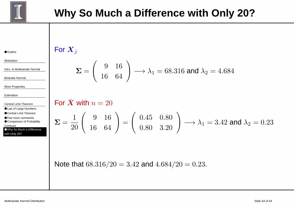
Why So Much a Difference with Only 20?

For Xj

Σ =

(

9 16

16 64

)

−→ λ1 = 68.316 and λ2 = 4.684

For X with n = 20

Σ =1

20

(

9 16

16 64

)

=

(

0.45 0.80

0.80 3.20

)

−→ λ1 = 3.42 and λ2 = 0.23

Note that 68.316/20 = 3.42 and 4.684/20 = 0.23.

Documents

The Multivariate Normal Distribution Edps/Soc 584 and ...courses.education.illinois.edu/EdPsy584/lectures/Multivariate... · Multivariate Normal Distribution Slide 1 of 54 The Multivariate