Efficient Gibbs Sampling of Truncated

Multivariate Normal with Application to

Constrained Linear Regression

Gabriel Rodriguez-Yam, Richard A. Davis, and Louis L. Scharf∗

March, 2004

Abstract

In this paper we propose an efficient Gibbs sampler for simulation of a

multivariate normal random vector subject to inequality linear constraints.

Inference in a Bayesian linear model, where the regression parameters are

subject to inequality linear constraints, is the primary motivation behind

this research. In the literature, implementations of the Gibbs sampler for the

multivariate normal distribution subject to inequality linear constraints and

for the multiple linear regression with inequality constraints often exhibit

poor mixing and slow convergence. This paper overcomes these limitations

∗ Gabriel Rodriguez-Yam is postdoctoral fellow and Richard Davis is Professor and chair,

Department of Statistics, Colorado State University, Fort Collins, CO. 80523-1877 (email:

rdavis@stat.colostate.edu). Louis Scharf is Professor, Departments of Electrical and Computer

Engineering and Statistics, Colorado State University, Fort Collins, CO, 80523-1877 (email:

scharf@engr.colostate.edu). This work forms part of the PhD dissertation of Gabriel Rodriguez-

Yam, supported in part part by Colorado Advanced Software Institute (CASI) and received a

scholarship from Consejo Nacional de Ciencia y Tecnologia (CONACYT). The work of Richard

Davis was supported in part by NSF grant DMS-0308109.

1

and, in addition, allows for the number of constraints to exceed the vector

size and is able to cope with equality linear constraints.

KEY WORDS: Bayesian, Markov chain Monte Carlo, inequality linear constraints.

1 Introduction

In the classical linear model

Y = Xβ + ε, (1)

where Y = [Y1, ..., Yn]T is the data vector, X is an n×k (n > k) design matrix having

full rank, ε is a vector of errors that are independent and N(0, σ2) distributed, and

β is the vector of regression parameters. The maximum likelihood estimate of β,

which coincides with the least squares estimator, is multivariate normal. Often

times, there are applications in which inequality constraints are placed on β. For

example, in hyperspectral imaging, the spectrum signature of a composite substance

in a pixel can be analyzed with the model in (1), where the columns of X are

the spectra of the k materials in the pixel (see Manolakis and Shaw 2002). Due

to physical considerations, the components of β, the abundance parameters, are

required to be non-negative, i.e., β ≥ 0. This example fits into the more general

framework where the vector β is subject to a set of inequality linear constraints

which can be written as

Bβ ≤ b. (2)

As long as the set defined in (2) has positive Lebesgue measure, there is a positive

probability that the least squares estimator of β may not satisfy the constraints.

When it does, it coincides with the maximum likelihood estimate as in the un-

constrained case. Except in simple cases, it is very difficult to obtain sampling

properties of the inequality restricted least squares estimator of β.

2

Judge and Takayama (1966) and Liew (1976) give the inequality constrained

least-squares (ICLS) estimate of β using the Dantzig-Cottle algorithm. The ICLS

estimator reduces to the ordinary least squares estimator for a sufficiently large

sample. Conditioned on knowing which constraints are binding and which are not

they compute an untruncated covariance matrix of the ICLS estimator. Geweke

(1986) points out that this variance matrix is incorrect, since in practice it is not

known ahead of time which constraints will be binding. Thus, inferences based on

this matrix can be seriously misleading (Lovell and Prescott 1970).

In this paper, we consider a Bayesian approach to this constrained inference

problem. Geweke (1986) uses a prior that is the product of a conventional unin-

formative distribution and an indicator function representing the inequality con-

straints. The posterior distribution and expected values of functions of interest are

then computed using importance sampling. In this case, an importance function

is easy to find due to the simplicity of the prior. However, this method can be

extremely slow, especially when the truncation region has a small probability with

respect to the unconstrained posterior distribution.

Gelfand, Smith and Lee (1992) suggest an approach to routinely analyze prob-

lems with constrained parameters using the Gibbs sampler, a Monte Carlo Markov

chain (MCMC) technique. Let D denote the data and θ a parameter vector with

some prior distribution. Suppose it is difficult or impossible to draw samples from

the posterior distribution p(θ|D). The Gibbs sampler, introduced by Geman and

Geman (1984) in the context of image restoration, provides a method for generat-

ing samples from p(θ|D). Suppose θ can be partitioned as θ = (θ1, . . . , θq), where

the θi’s are either uni- or multidimensional and that we can simulate from the

conditional posterior densities p(θi|D,θj, j 6= i). The Gibbs sampler generates a

Markov chain by cycling through p(θi|D,θj, j 6= i). In each cycle, the most recent

information updates the posterior conditionals. Starting from some θ(0), after t cy-

3

cles we have a realization θ(t) that under regularity conditions (Gelfand and Smith

1990), approximates a drawing from p(θ|D) for large t. O’Hagan (1994), Gilks and

Roberts (1996), Roberts (1996) comment that the rate of convergence depends on

the posterior correlation between the components of the vector θ.

Geweke (1996) implements the Gibbs sampler for the problem of multiple linear

regression with at most k independent inequality linear constraints given by

c ≤ Bβ ≤ d, (3)

where B is a square matrix of full rank, c < d and the elements of c and d are

allowed to be −∞ and +∞, respectively. Notice that these constraints can be

easily rewritten in the form given in (2). However, Geweke’s implementation may

suffer from poor mixing (i.e., the chain does not move rapidly through the “entire”

support of the posterior distribution). In our implementation we do not impose any

limitation on the number of constraints given in (2). A major difference however, is

that our implementation has faster mixing, requiring substantially fewer iterations

of the Markov chain than previously published Gibbs sampler implementations.

In Rodriguez-Yam, Davis and Scharf (2002), a Gibbs sampler implementation

with good mixing is provided for the hyperspectral imaging problem when only the

non-negativity constraints on the abundance parameters are considered. For this

case, the constraints are linearly independent and the number of inequality linear

constraints coincides with the number of regression coefficients.

The organization of this paper is as follows. In Section 2 we provide a Bayesian

framework for multiple linear regression where the regression parameters are sub-

ject to the constraints in (2). In Section 3 we list standard results for the truncated

multivariate normal distribution that are used in this paper and provide an efficient

Gibbs sampler from this distribution. Through an example where the constraints

can be written as in (3) we compare our implementation with that of Geweke’s.

In Section 4 we use the implementation from Section 3 to provide an implementa-

4

tion of the Gibbs sampler to the model in Section 2 and apply the procedure to

two datasets. One is the rental data analyzed by Geweke (1986, 1996) where the

regression coefficients are subject to a set of inequality linear constraints that can

be written as in (3). The other is aggregate data involving smokers preferences of

three leading brands of cigarettes. For this example, equality linear constraints are

needed in addition to inequality linear constraints and the number of inequality

linear constraints exceeds the number of regression coefficients. Section 5 contains

a summary of our findings.

2 Constrained Linear Regression

In this section we construct a Bayesian model for the multiple linear regression

given in (1) where the parameters satisfy the constraints in (2). Before doing this,

we introduce our notation. If R is a subset of <k having positive Lebesgue measure,

we call the random k-vector Y truncated normal and write Y ∼ NR(µ,Σ) if its

probability density function is proportional to φ(x; µ,Σ)IR(x), where φ(x; µ,Σ) is

the k-variate normal density with mean µ and covariance matrix Σ, and IR(.) is

the indicator function for R.

Now, the inequality linear constraints in (2) define a subset of <k given by

T := {β ∈ <k : Bβ ≤ b}. (4)

Notice that the model in (1) describes the conditional distribution of Y given the

vector of parameters θ := (β, σ2), consisting of the coefficients of regression and

the common variance of the noise errors. Now assume the prior for θ is given by

β ∼ NT (µ0, σ20(X

TX)−1), (5)

σ2 ∼ IG(ν, λ), (6)

where β and σ2 are independently distributed, σ20, ν and λ are known positive

scalars and µ0 is a known vector. If p(β, σ2|y) denotes the posterior distribution

5

of θ given the observed vector y, then,

p(β, σ2|y) ∝ L(β, σ2;y)p(β)p(σ2) (7)

where L(β, σ2;y) is the likelihood function based on the data y from the model

in (1). A sample from the posterior density p(β, σ2|y) will allow us to compute

posterior quantities, such as means, variances, probabilities, and so on. In Section

4 below we describe how to obtain such a sample.

3 Truncated Multivariate Normal Distribution

In order to have an efficient Gibbs sampler for the multiple linear regression problem

with inequality linear constraints as given in (4), it is imperative to have an efficient

sampler to the truncated multivariate normal distribution. Before pursuing this ob-

jective we begin by developing two properties of the truncated multivariate normal

distribution and then propose an implementation of the Gibbs sampler for the mul-

tivariate normal distribution subject to a set of inequality linear constraints. A key

feature of this implementation is the construction of variables that are independent

when the constraints are ignored. Using the first example from Geweke (1991), the

performance of our implementation is then compared with that of Geweke’s.

For a multivariate normal random vector X, all linear transformations and con-

ditional distributions of X are normal. It turns out that for a truncated normal

vector, these closure properties remain valid. That is, a linear transformation of a

truncated normal vector is also truncated normal and so are the one-dimensional

conditional distributions. These conditional distributions play a key role in the

implementation of the Gibbs sampler we propose. The specifics are as follows:

Result 1 (a) Suppose X ∼ NR(µ,Σ), where R ∈ <k has positive Lebesgue mea-

sure, and Σ is positive definite. Let Y := AX, where A is a matrix of full rank of

6

dimension r × k with r ≤ k. Then,

Y ∼ NT (Aµ,AΣAT ), T := {Ax : x ∈ R}. (8)

(b) Partition X, µ and Σ as

X =

X1

Xk

, µ =

µ1

µk

, Σ =

Σ11 Σ1

ΣT1 σkk

. (9)

Then,

Xk|X1 = x1 ∼ NRk(µ∗k, σ

∗kk), (10)

where

µ∗k = µk + ΣT1 Σ−1

11 (x1 − µ1), (11)

σ∗kk = σkk −ΣT1 Σ−1

11 Σ1, (12)

Rk := {xk ∈ < : (x1, xk) ∈ R}. (13)

The proof of (a) is immediate from the form of the density function for truncated

normal random vectors. To prove (b) the expressions for the inverse of a par-

titioned symmetric matrix (in Hocking 1996) are used, from which the result is

immediate. ¤

Gibbs Sampler

Suppose θ is a vector of parameters with posterior distribution p(θ|D), where Ddenotes the data. Partition θ as (θ1, . . . , θq), where the θi’s are either uni- or

multidimensional in such a way that we can simulate from the conditional pos-

terior densities p(θi|D,θj, j 6= i). The basic Gibbs sampler starts with an ini-

tial value θ(0) = (θ(0)1 , . . . , θ(0)

q ) from the support of p(θ|D) and then generates

θ(t) = (θ(t)1 , . . . , θ(t)

q ), t=1, 2, . . ., recursively as follows:

Generate θ(t)1 from p(θ1|D, θ

(t−1)2 , . . . , θ(t−1)

q )

7

Generate θ(t)2 from p(θ2|D, θ

(t)1 ,θ

(t−1)3 , . . . , θ(t−1)

q )

...

Generate θ(t)q from p(θq|D, θ

(t)1 , θ

(t)2 , . . . , θ

(t)q−1).

Under certain regularity conditions (e.g. Gelfand and Smith 1990) the Markov chain

{θ0,θ1,θ2, . . .} has a stationary distribution which is the posterior distribution

p(θ|D).

3.1 Gibbs sampler implementations

For comparison purposes, we first describe the implementation of the Gibbs sampler

given by Geweke (1991) to a truncated normal random vector of dimension k subject

to a set of at most k linearly independent inequality linear constraints. Suppose

that X is a truncated normal random vector of dimension k, such that

X ∼ NT (µ, σ2Σ), T := {x ∈ <k : c ≤ Bx ≤ d}, (14)

where c, d and B are as in (3).

The Gibbs sampler in Geweke’s implementation is applied to the transformed

random vector Y = BX. Note that

Y ∼ NS(Bµ, σ2BΣBT ), S = {y ∈ <k : c ≤ y ≤ d}. (15)

Thus, using (10)

Yj|(Y1 = y1, . . . , Yj−1 = yj−1, Yj+1 = yj+1, . . . , Yk = yk) ∼ NSj(µ∗j , σ

∗jj), (16)

where Sj = {yj ∈ < : cj ≤ yj ≤ dj}, and µ∗j and σ∗jj must be obtained as in (11)

and (12), respectively. Geweke’s implementations, which we call Sampler TN1, is

then

8

Sampler TN1 (Geweke 1991)

Update the last component y(t) = [y(t)1 , y

(t)2 , . . . , y

(t)k ]T of the current Gibbs path

y(0),y(1), . . . ,y(t), as follows: for j = 1, . . . , k

• draw y(t+1)j from p(yj|y(t+1)

1 , . . . , y(t+1)j−1 , y

(t)j+1, . . . , y

(t)k ), (17)

where each conditional distribution is given in (16). ¤

The sampler we now propose allows for the number of constraints to exceed k.

Begin with

X ∼ NT (µ, σ2Σ), T := {x ∈ <k : Bx ≤ b}, (18)

where the rows of the matrix B are not restricted to be linearly independent. Let

A be a square matrix of full rank, such that AΣAT = I, where I is the identity

matrix and set

Z := AX. (19)

From (a) of Result 1, it follows that

Z ∼ NS(Aµ, σ2I), S = {Ax : x ∈ <k,Bx ≤ b}. (20)

The set S can be rewritten in the more suggestive way,

S = {z ∈ <k,Dz ≤ b}, (21)

where

D := BA−1. (22)

Thus, the transformation in (19) simplifies the functional form of the truncated

multivariate distribution, but not the constraints.

If α := Aµ, and Z−j and z−j denote the vectors [Z1, . . . , Zj−1, Zj+1, . . . , Zk]T

and [z1, . . . , zj−1, zj+1, . . . , zk]T , respectively, then by (b) of Result 1,

Zj|Z−j = z−j ∼ NSj(αj, σ2), (23)

9

where from (13) and (21)

Sj = {zj ∈ < : z ∈ S} = {zj ∈ < : Dz ≤ b}.

Let D−j be the matrix obtained from D = [d1 . . .dk] by removing the j-th column.

Then the set Sj can be easily computed from the equation

Sj = {zj ∈ < : djzj ≤ b−D−jz−j}. (24)

Since the constraints on X form a convex subset of <k, the set Sj in (24) can be

written as one of the intervals lj ≤ zj ≤ uj, −∞ < zj ≤ uj or lj ≤ ηj < +∞. The

values lj and uj can be easily obtained from the set of one-dimensional inequalities

in (24).

The idea behind the transformation in (19) is to obtain an efficient implemen-

tation of the Gibbs sampler based on the set of k conditional distributions in (23).

These distributions have a simple form. That is, once the transformed mean α has

been obtained, we do not need to use equations like (11) and (12) to compute the

k means and variances. Also, the one-dimensional truncation intervals Sj in (24)

evolve simply.

To illustrate this process, consider the following example. Let X ∼ NT (µ, σ2Σ),

where

T = {x ∈ <2 : x ≥ 0}, and Σ =

1 4/5

4/5 1

.

Notice that in the notation in (4), B = −I and b = 0, where I is the identity

matrix. For the lower-triangular Cholesky factor A of Σ given by

A =

1 0

−4/3 5/3

,

we obtain AΣAT = I. The matrix D = BA−1 given in (22), and the submatrices

D−1 and D−2, are

D =

−1 0

−4/5 −3/5

, D−1 =

0

−3/5

, D−2 =

−1

−4/5

.

10

Then,

Z1|Z−1 = z−1 ∼ NS1(µ1, σ2), Z2|Z−2 = z−2 ∼ NS2(−4

3µ1 +

5

3µ2, σ2),

where

S1 = {z1 ∈ < :

−1

−4/5

z1 ≤ −

0

−3/5

z2}

= {z1 ∈ < : z1 ≥ 0; z1 ≥ −3

4z2}

= [max{0,−3

4z2},∞)

S2 = {z2 ∈ < :

0

−3/5

z2 ≤ −

−1

−4/5

z1}

= {z2 ∈ < : z2 ≥ −4

3z1}

= [−4

3z1,∞).

For this example, the matrix B needed in (14) is the identity I. Hence, in Sampler

TN1, the Gibbs sampler is implemented on the random vector X. In particular,

using (11)-(12) in (16), it follows that

Y1|Y2 = y2 ∼ NS1(µ1 +4

5(y2 − µ2)σ

2,9

25σ2),

Y2|Y1 = y1 ∼ NS2(µ2 +4

5(y1 − µ1)σ

2,9

25σ2)

where S1 = S2 = [0, +∞). ¤

Now, to obtain a sample from the distribution of X we obtain first a sample

from the transformed vector Z in (19). A sample from X is then obtained by “un-

doing” this transformation. For later reference this new implementation will be

called Sampler TN2.

11

Sampler TN2 (This paper)

Let z0 ∈ S be an initial value of the sampler. The last component z(t) = [z(t)1 , z

(t)2 ,

. . . , z(t)k ]T of the current Gibbs path z(0), z(1), . . . , z(t) is updated as follows:

• draw z(t+1)j from p(zj|z(t+1)

1 , . . . , z(t+1)j−1 , z

(t)j+1, . . . , z

(t)k ), j = 1, . . . , k,

• set X(t+1) = A−1Z(t+1),

where the conditional distribution p(zj|z(t+1)1 , . . . , z

(t+1)j−1 , z

(t)j+1, . . . , z

(t)k ) is given in

(23). ¤

3.2 Performance comparison of Samplers TN1 and TN2

To compare the performance between Samplers TN1 and TN2, we consider an

example in which X ∼ NT (µ,Σ), where

µ =

0

0

, Σ =

10 ρ

ρ 0.1

, (25)

and T is the region determined by the constraints,

c1 ≤ X1 + X2 ≤ d1, c2 ≤ X1 −X2 ≤ d2. (26)

These constraints can be written in the format in (14) with c = [c1 c2]T , d = [d1 d2]

T

and

B =

1 1

1 −1

.

To provide some indication of the efficiency of his procedure, Geweke (1991) con-

sidered five configurations of truncation points of c1, c2, d1 and d2 (and ρ = 0). In

this paper we consider three configurations of truncation points of c1, c2, d1 and

d2 and three values of ρ. For each configuration we apply the two Gibbs sampler

implementations described above and stop after 1600 iterations. As a means of

12

comparison of the two implementations, the results of the Raftery and Lewis con-

vergence diagnostic procedure for each chain are shown in Tables 1 and 2. In the

general set up of the Gibbs sampler, this diagnostic, introduced by Raftery and

thinning lower dependence

ρ variable (k) burn-in Total bound factor

−∞ < X1 + X2 < ∞, −∞ < X1 −X2 < ∞-0.7 X1 23 115 58282 1537 37.92

X2 3 12 6726 1537 4.37

0 X1 18 90 46206 1537 30.06

X2 1 2 1551 1537 1.01

0.7 X1 22 154 72050 1537 23.96

X2 3 12 6549 1537 5.89

−10 ≤ X1 + X2 ≤ 10, −10 ≤ X1 −X2 ≤ 10

-0.7 X1 25 150 78650 1537 51.17

X2 6 24 14160 1537 9.21

0 X1 10 60 30040 1537 19.54

X2 1 2 1558 1537 1.01

0.7 X1 20 120 60380 1537 39.28

X2 6 24 13272 1537 8.64

−1 ≤ X1 + X2 ≤ 1, −1 ≤ X1 −X2 ≤ 1

-0.7 X1 3 12 6087 1537 3.96

X2 1 3 1397 1537 0.91

0 X1 2 6 3436 1537 2.24

X2 1 3 1312 1537 0.85

0.7 X1 3 12 5976 1537 3.89

X2 1 3 1329 1537 0.86

Table 1: Raftery and Lewis convergence diagnostics for Sampler TN1 implemented on the

truncated normal random vector [X1, X2]T with unconstrained mean 0, var{X1} = 10,

var{X2} = 0.10 and cor{X1, X2} = ρ, subject to the constraints c1 ≤ X1+X2 ≤ d1, c2 ≤X1 −X2 ≤ d2.

13

thinning lower dependence

ρ variable (k) burn-in Total bound factor

−∞ < X1 + X2 < ∞, −∞ < X1 −X2 < ∞-0.7 X1 1 3 1702 1537 1.11

X2 1 2 1501 1537 0.98

0 X1 1 2 1432 1537 0.93

X2 1 2 1582 1537 1.03

0.7 X1 1 2 1505 1537 0.98

X2 1 2 1516 1537 0.99

−10 ≤ X1 + X2 ≤ 10, −10 ≤ X1 −X2 ≤ 10

-0.7 X1 1 2 1490 1537 0.97

X2 1 2 1566 1537 1.02

0 X1 1 2 1509 1537 0.98

X2 1 2 1490 1537 0.97

0.7 X1 1 2 1614 1537 1.05

X2 1 3 1689 1537 1.10

−1 ≤ X1 + X2 ≤ 1, −1 ≤ X1 −X2 ≤ 1

-0.7 X1 1 2 1566 1537 1.02

X2 1 2 1450 1537 0.94

0 X1 1 3 1390 1537 0.90

X2 1 2 1520 1537 0.99

0.7 X1 1 2 1655 1537 1.08

X2 1 2 1531 1537 1.00

Table 2: Raftery and Lewis convergence diagnostics for Sampler TN2 implemented on

the truncated bivariate normal random vector [X1, X2]T described in Table 1.

Lewis (1992), determines the total number of iterations required to compute quan-

tiles of functionals of θ. Also, the method gives the number of initial iterations

that must be discarded to allow for “burn-in”. Some specifics of the method are

as follows. Let ξ be a function of the parameter vector θ. For a fixed probability

s, a known q and accuracy r, suppose that we want to estimate the value of the

14

quantile u, given by P (ξ ≤ u|D) = q in such a way that P (|q̂ − q| ≤ r|D) = s,

where q̂ is an estimator of q based on the sample path of the chain.

In Tables 1 and 2, the columns labeled “bound” would be the total length

needed if the components of the chain were in fact an iid sample. The column

labeled as “thinning” means that after the burn-in, every k-th observation is used.

In both tables we set q = 0.5, r = 0.025 and s = 0.95. Based on the results from

these tables, we note that the convergence of Sampler TN1 is much slower than

that for Sampler TN2. Also, ρ (which is the correlation between X1 and X2 when

no truncation is considered) affects the performance of Sampler TN1. In general,

as the region of truncation gets small, the speed of convergence of Sampler TN1

improves. One possible explanation for this is that the chain must cover a “small”

region faster than a “large” region. On the other hand, Sampler TN2 has the

advantage of providing samples that are “close” to iid samples, regardless of the

size of the region of truncation or the correlation of X1 and X2. In fact, for the

configuration −∞ < X1 + X2 < ∞, −∞ < X1 −X2 < ∞, this sampler provides

an iid sample, since the conditional distribution in (23) does not depend on the

fixed values z−j (e.g., see O’Hagan 1994, p. 233).

The autocorrelations of the output of a Gibbs sampler can be used to measure

the performance of a simulation. Chen, Shao and Ibrahim (2000) observe that slow

decay in the autocorrelations suggests slow mixing within a chain and usually slow

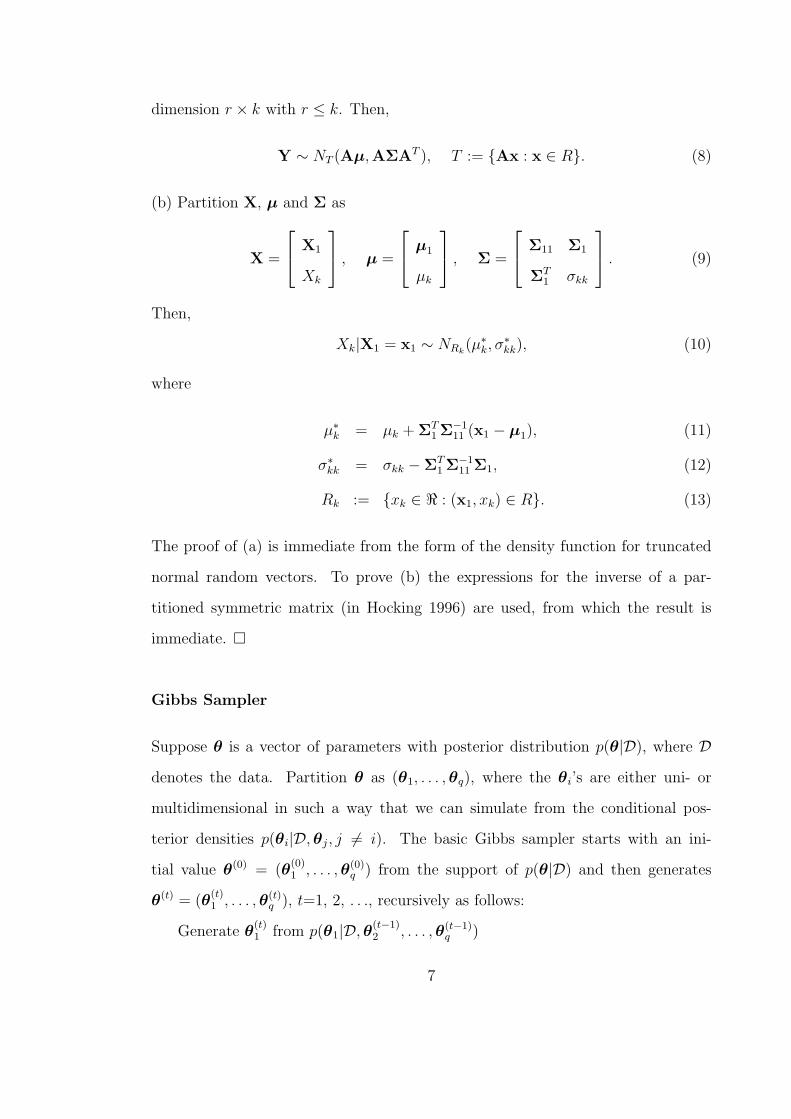
convergence to the posterior distribution. For this example, the autocorrelations of

X1, X2 and X1 +X2 for two configurations of values of ρ, c and d using the output

of the Sampler TN1 are shown in Figure 1. The first row of graphs contains the

autocorrelations for ρ = 0, −∞ < X1 +X2 < ∞, and −∞ < X1−X2 < ∞ and the

second row of graphs contains the autocorrelations for ρ = −0.7, −1 ≤ X1+X2 ≤ 1

and −1 ≤ X1 −X2 ≤ 1. Figure 2 contains the analogous autocorrelations for the

output of Sampler TN2. For the two configurations considered in Figures 1 and 2,

15

lag

auto

corre

latio

n

X1

0 10 20 30-1

.0-0

.50.

00.

51.

0lag

auto

corre

latio

n

X2

0 10 20 30

-1.0

-0.5

0.0

0.5

1.0

lag

auto

corre

latio

n

X1+X2

0 10 20 30

-1.0

-0.5

0.0

0.5

1.0

lag

auto

corre

latio

n

X1

0 10 20 30

-1.0

-0.5

0.0

0.5

1.0

lag

auto

corre

latio

n

X2

0 10 20 30-1

.0-0

.50.

00.

51.

0lag

auto

corre

latio

n

X1+X2

0 10 20 30

-1.0

-0.5

0.0

0.5

1.0

Figure 1: Autocorrelation plots of X1, X2 and X1 + X2 for two configurations of values

of ρ, c and d obtained with Sampler TN1.

lag

auto

corre

latio

n

X1

0 10 20 30

-1.0

-0.5

0.0

0.5

1.0

lag

auto

corre

latio

n

X2

0 10 20 30

-1.0

-0.5

0.0

0.5

1.0

lag

auto

corre

latio

n

X1+X2

0 10 20 30

-1.0

-0.5

0.0

0.5

1.0

lag

auto

corre

latio

n

X1

0 10 20 30

-1.0

-0.5

0.0

0.5

1.0

lag

auto

corre

latio

n

X2

0 10 20 30

-1.0

-0.5

0.0

0.5

1.0

lag

auto

corre

latio

n

X1+X2

0 10 20 30

-1.0

-0.5

0.0

0.5

1.0

Figure 2: Autocorrelation plots of X1, X2 and X1 + X2 for two configurations of values

of ρ, c and d obtained with Sampler TN2.

we conclude that the mixing of the Sampler TN2 is better than that of the Sampler

TN1. Notice that the column labeled “dependence factor” in Tables 1 and 2 is

16

related to the mixing provided by the autocorrelation plots in Figures 1 and 2.

That is, the slower the mixing, the higher the dependence factor and vice versa.

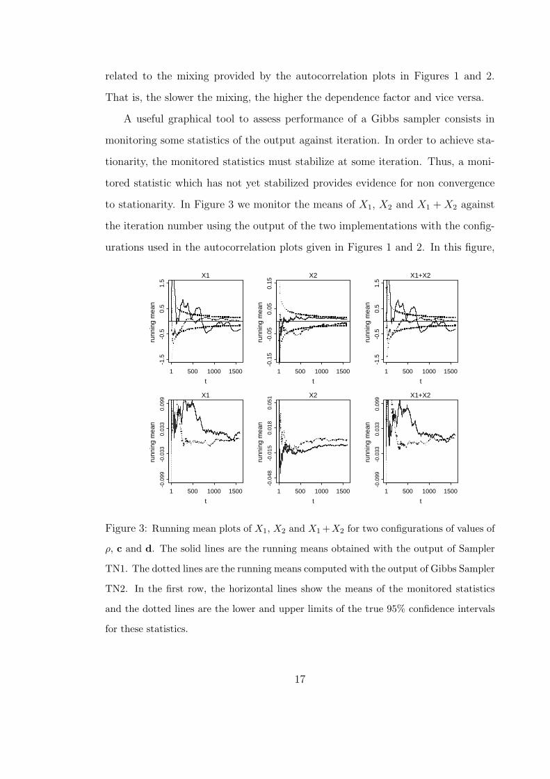
A useful graphical tool to assess performance of a Gibbs sampler consists in

monitoring some statistics of the output against iteration. In order to achieve sta-

tionarity, the monitored statistics must stabilize at some iteration. Thus, a moni-

tored statistic which has not yet stabilized provides evidence for non convergence

to stationarity. In Figure 3 we monitor the means of X1, X2 and X1 + X2 against

the iteration number using the output of the two implementations with the config-

urations used in the autocorrelation plots given in Figures 1 and 2. In this figure,

t

runn

ing

mea

n

X1

1 500 1000 1500

-1.5

-0.5

0.5

1.5

t

runn

ing

mea

n

X2

1 500 1000 1500

-0.1

5-0

.05

0.05

0.15

t

runn

ing

mea

n

X1+X2

1 500 1000 1500-1

.5-0

.50.

51.

5

t

runn

ing

mea

n

X1

1 500 1000 1500

-0.0

99-0

.033

0.03

30.

099

t

runn

ing

mea

n

X2

1 500 1000 1500

-0.0

48-0

.015

0.01

80.

051

t

runn

ing

mea

n

X1+X2

1 500 1000 1500

-0.0

99-0

.033

0.03

30.

099

Figure 3: Running mean plots of X1, X2 and X1 +X2 for two configurations of values of

ρ, c and d. The solid lines are the running means obtained with the output of Sampler

TN1. The dotted lines are the running means computed with the output of Gibbs Sampler

TN2. In the first row, the horizontal lines show the means of the monitored statistics

and the dotted lines are the lower and upper limits of the true 95% confidence intervals

for these statistics.

17

the solid lines are the means obtained using the output of Sampler TN1, while the

dotted lines are the means obtained with the output of Sampler TN2. Recall that

Sampler TN2 provides an iid sample X(1), X(2), . . ., X(t) from the distribution of

X when −∞ < X1 + X2 < ∞, −∞ < X1 − X2 < ∞. Thus, the means and

variances of X̄1, X̄2 and X̄1 + X̄2 (which are estimators of the means of X1, X2 and

X1 + X2, respectively) are known. For example, E(X̄1) = 0 and var(X̄1) = 10/t.

In the first row of Figure 3, the horizontal solid lines show the expected means

of the monitored statistics, while the dotted lines show the upper and lower 95%

confidence limits ∓1.96σ of the monitored statistics. We note in this figure that the

monitored means stabilize earlier for the Sampler TN2. In particular, in the upper

left panel, with Sampler TN2, the monitored means stabilize after 500 iterations,

while for Sampler TN1 they have not yet stabilized even after 1500 iterations.

4 Gibbs Sampler Implementations to the Con-

strained Linear Regression

In this section we implement the Gibbs sampler for a Bayesian linear regression

model in which the regression coefficients satisfy inequality linear constraints. When

the number of constraints does not exceed the number of regression coefficients we

compare our procedure with the implementation described in Geweke (1996). In

addition, we show through an example how the case of equality linear constraints

can be handled.

Combining the prior distribution of (β, σ2) given in (5)-(6) with the likelihood

of the model in (1) we have

β|(σ2,y) ∼ NT (µ1,Σ1) (27)

σ−2|(β,y) ∼ (SS(β) + 2λ)−1χ2n+2ν , (28)

where χ2n+2ν denotes a chi-squared distribution with n + 2ν degrees of freedom, T

18

is defined in (4), and

µ1 = γβ̂ + (1− γ)µ0

Σ1 = σ2γ(XTX)−1

SS(β) = (y −Xβ)T (y −Xβ)

γ = σ20/(σ

20 + σ2)

β̂ = (XTX)−1XTy.

To show (27) and (28), an analogous procedure for the unconstrained linear model

(e.g., Tanner 1996, pp. 17-18) can be followed.

For comparison purposes, we describe now the implementation of the Gibbs

sampler given by Geweke (1996) for a multiple linear regression model where the

regression coefficients are subject to a set of at most k linearly independent inequal-

ity linear constraints. That is,

T := {β ∈ <k : c ≤ Bβ ≤ d},

where c, d and B are as in (3).

As in Sampler TN1, the vector of regression coefficients β is transformed to

η = Bβ. Then,

η|(σ2,y) ∼ NS(Bµ1,BΣ1BT ), S = {β ∈ <k : c ≤ β ≤ d}. (29)

The full implementation of the Gibbs sampler to the vector θ := (η, σ2) proposed

by Geweke is summarized in the following sampler.

Sampler CLR1

Let θ(0),θ(1), . . . , θ(t) be the current path of the Gibbs sampler. The last component

θ(t) = (η(t)1 , . . . , η

(t)k , σ2(t)) is updated as follows:

• Generate η(t+1)1 from p(η1|η(t)

2 , . . . , η(t)k , σ2(t),y)

19

• Generate η(t+1)2 from p(η2|η(t+1)

1 , η(t)3 . . . , η

(t)k , σ2(t),y)

...

• Generate η(t+1)k from p(ηk|η(t+1)

1 , η(t+1)2 . . . , η

(t+1)k−1 , σ2(t),y)

• Generate σ2(t+1) from p(σ2|η(t+1)1 , η

(t+1)2 . . . , η

(t+1)k ,y),

where, due to (29), for j = 1, . . . , k, the distribution

p(ηj|η(t+1)1 , . . . , η

(t+1)j−1 , η

(t)j+1, . . . , η

(t)k , σ2(t),y),

is univariate normal truncated below by ci, truncated above by di, and its mean

and variance found using (29) along with the expressions in (11) and (12). Also,

p(σ2|η(t+1)1 , η

(t+1)2 . . . , η

(t+1)k ,y) can be obtained from (28). ¤

Now, we give a new implementation, similar to Sampler TN2, for the case where

the number of inequality linear constraints can exceed the number of regression

parameters. For this case, T is given in (4). Let A be a non-singular matrix for

which A(XTX)−1A = I, and set

η = Aβ. (30)

Then, from (8) and (27)

η|(σ2,y) ∼ NS(Aµ1, σ2γI), S = {η ∈ <k : Dη ≤ b}, (31)

where D = BA−1 and B and b are defined as in (2). We implement the Gibbs sam-

pler for the transformed vector θ = (η, σ2). The details are given in Sampler CLR2.

Sampler CLR2

Update the last component θ(t) = (η(t)1 , . . . , η

(t)k , σ2(t)) of the current path θ(0), θ(1),

. . ., θ(t) of the Gibbs sampler as follows

20

• Generate η(t+1)1 from p(η1|η(t)

2 , . . . , η(t)k , σ2(t),y)

• Generate η(t+1)2 from p(η2|η(t+1)

1 , η(t)3 . . . , η

(t)k , σ2(t),y)

...

• Generate η(t+1)k from p(ηk|η(t+1)

1 , η(t+1)2 . . . , η

(t+1)k−1 , σ2(t),y)

• Generate σ2(t+1) from p(σ2|η(t+1)1 , η

(t+1)2 . . . , η

(t+1)k ,y),

where due to (31), for j = 1, . . . , k, the distribution

p(ηj|η(t+1)1 , . . . , η

(t+1)j−1 , η

(t)j+1, . . . , η

(t)k , σ2(t),y),

can be obtained similarly as in Sampler TN2, and p(σ2|η(t+1)1 , η

(t+1)2 . . . , η

(t+1)k ,y)

can be obtained from (28). ¤

4.1 Example: Rental Data

We consider the 32 observations provided by Pindyck and Rubinfeld (1981, p. 44)

on rent paid, number of rooms rented, number of occupants, sex and distance from

campus in blocks for undergraduates at the University of Michigan. Geweke (1986,

1996) considers the model

yi = β1 + β2siri + β3(1− si)ri + β4sidi + β5(1− si)di + εi,

where yi denotes rent paid per person, ri number of rooms per person, di distance

from campus in blocks, si is a dummy variable representing gender (one for male

and zero for female), εi is normally distributed error with mean 0 and variance σ2,

and the β’s are subject to the constraints

β2 ≥ 0, β3 ≥ 0, β4 ≤ 0, β5 ≤ 0. (32)

Since the number of constraints does not exceed the number of regression coef-

ficients, Sampler CLR1 can be used to draw a sample from the posterior dis-

tribution of (β, σ2). For this case, the matrix B is the identity of size 5, c :=

21

[−∞, 0, 0,−∞,−∞]T and d := [∞,∞,∞, 0, 0]T . For Sampler CLR2, b = 0 and B

is given by

B =

0 −1 0 0 0

0 0 −1 0 0

0 0 0 1 0

0 0 0 0 1

.

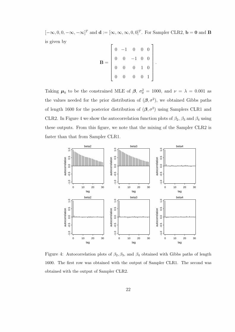
Taking µ0 to be the constrained MLE of β, σ20 = 1000, and ν = λ = 0.001 as

the values needed for the prior distribution of (β, σ2), we obtained Gibbs paths

of length 1600 for the posterior distribution of (β, σ2) using Samplers CLR1 and

CLR2. In Figure 4 we show the autocorrelation function plots of β2, β3 and β4 using

these outputs. From this figure, we note that the mixing of the Sampler CLR2 is

faster than that from Sampler CLR1.

lag

auto

corr

elat

ion

beta2

0 10 20 30

-1.0

-0.5

0.0

0.5

1.0

lag

auto

corr

elat

ion

beta3

0 10 20 30

-1.0

-0.5

0.0

0.5

1.0

lag

auto

corr

elat

ion

beta4

0 10 20 30

-1.0

-0.5

0.0

0.5

1.0

lag

auto

corr

elat

ion

beta2

0 10 20 30

-1.0

-0.5

0.0

0.5

1.0

lag

auto

corr

elat

ion

beta3

0 10 20 30

-1.0

-0.5

0.0

0.5

1.0

lag

auto

corr

elat

ion

beta4

0 10 20 30

-1.0

-0.5

0.0

0.5

1.0

Figure 4: Autocorrelation plots of β2, β3, and β4 obtained with Gibbs paths of length

1600. The first row was obtained with the output of Sampler CLR1. The second was

obtained with the output of Sampler CLR2.

22

To compare the speed of convergence of both samplers, we increased the length

of both paths to a total length of 20000 (each path). In Figure 5 we show two

sections of the running mean plots of σ2 and all the components of β. In each

panel, the thick lines correspond to the section 9401 ≤ t ≤ 10000 while the thin

lines correspond to the section 19401 ≤ t ≤ 20000. The solid lines were obtained

using the output of Sampler CLR1 and the dotted lines using the output of Sampler

CLR2. While it appears that for Sampler CLR2, 20000 iterations are enough to

stabilize the mean of σ2 and β, this is not the case for Sampler CLR1.

t

run

nin

g m

ea

n

beta1

9400 9600 9800 10000

36

.23

6.9

37

.6

t

run

nin

g m

ea

nbeta2

9400 9600 9800 10000

13

3.8

13

4.6

13

5.4

tru

nn

ing

me

an

beta3

9400 9600 9800 100001

23

.01

23

.81

24

.6

t

run

nin

g m

ea

n

beta4

9400 9600 9800 10000

-0.5

00

5-0

.49

78

-0.4

95

0

t

run

nin

g m

ea

n

beta5

9400 9600 9800 10000

-1.1

58

0-1

.15

55

-1.1

53

0

t

run

nin

g m

ea

n

sigma^2

9400 9600 9800 10000

15

33

15

37

15

41

Figure 5: Two sections of the running means of β1, . . . , β5 and σ2. The thick lines show

the first sections (9401 ≤ t ≤ 10000) and the thin lines the second sections (19401 ≤ t ≤20000) of these running means. The values obtained with the output of Sampler CLR1

are shown with solid lines and those obtained with the output of Sampler CLR2 with

dotted lines.

23

4.2 Example: Application to the Cigarette-brand Prefer-

ence Data

This example considers the estimation of the transition probability matrix of a finite

Markov process when only the time series of the proportion of visits to each state

is known. To estimate the transition probability matrix, Telser (1963), proposes

least-squares estimation based on a set of regression models subject to constraints

that the coefficients are non-negative and each row sums to 1. This problem is

analyzed again by Judge and Takayama (1966), who take these constraints into

account explicitly. The numerical example given by Telser (1963) and Jugde and

Takayama (1966), consists of the annual sales in billions of cigarettes for the three

leading brands from 1925 to 1943. Given the time ordered market shares of these

brands and assuming that the probability of a transition, pij, from brand i to brand

j is constant over time, Telser gives the regression models

yjt =3∑

i=1

yi,t−1pij + ujt, j = 1, 2, 3, (33)

where yjt is the proportion of individuals in state j at time t and ujt, t = 1, . . . , T

are independent errors. The probabilities pij are subject to the constraints

3∑j=1

pij = 1, for all i, (34)

pij ≥ 0, for all i, and j. (35)

For the cigarettes data, the three models in (33) can be combined as

y1

y2

y3

=

W 0 0

0 W 0

0 0 W

p1

p2

p3

+

u1

u2

u3

, (36)

where yj := [yj2, . . . , yjT ]T , W is the common design matrix of dimension 3×T −1

from the models in (33), pj is the j-th column of the probability transition matrix

24

P of the finite Markov process, and uj is the vector of errors from the model in

(33).

We propose to treat the equality constraints in (34) as in the frequentist ap-

proach. Hocking (1996, p. 70) incorporates equality linear constraints into the so

called full model to obtain a reduced model. For this Bayesian approach, a new

feature appears. The equality constraints need to be “incorporated” in the support

of the full model. Denote by y the response vector of the full model in (36), by

W1, W2 and W3 the matrices having the columns 1 through 3, 4 through 6 and 7

through 9, respectively of the design matrix in (36). Substituting pi3 = 1−pi1−pi2,

i = 1, 2, 3, in this model, we obtain

y −W3

1

1

1

= [W1 −W3 W2 −W3]

p1

p2

+ u, (37)

subject to the constraints

pi1 + pi2 ≤ 1, i = 1, 2, 3, (38)

pij ≥ 0, i = 1, 2, 3, j = 1, 2, (39)

where u is the vector of errors from the model in (36). In their method, Judge and

Takayama (1966) assume that var(u) = σ2I. For simplicity we also assume that

u ∼ N(0, σ2I). However, a more general matrix of variance-covariance for u can

be used, e.g., var{uj} = σ2j I and cov{uj1 ,uj2} = 0, j1 6= j2. For this case, a prior

distribution for the vector (σ21, σ

22, σ

23) needs to be specified.

Notice that the number of constraints in (38) and (39) to the regression model

in (37) exceeds the number of regression coefficients. This time, Sampler CLR1

can not be carried out. To implement the Sampler CLR2, set µ0 equal to the

constrained MLE of β := [pT1 pT

2 ], σ20 large (100), and ν = λ = 0.001 as the

values needed for the prior distribution of (β, σ2). A path of length 5000 for the

25

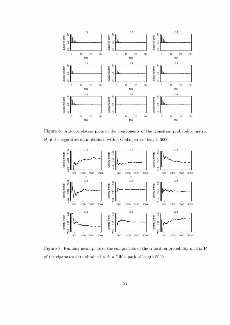
posterior distribution of (β, σ2) is then generated. Based on the last 2500 iterates

of this sample, the estimate P̂ of the probability transition matrix and the matrix

σ̂P̂ having in its entries the estimated standard error of each component of P̂ are

P̂ =

0.690 0.118 0.192

0.035 0.844 0.121

0.334 0.060 0.606

, (40)

σ̂P̂ =

0.0016 0.0009 0.0016

0.0006 0.0008 0.0009

0.0023 0.0010 0.0024

.

The restricted least-squares estimates obtained by Judge and Takayama (1966) are

given by

P̂ =

0.6686 0.1423 0.1891

0 0.8683 0.1317

0.4019 0 0.5981

. (41)

The estimates in (40) differ slightly from the restricted least-squares in (41). Per-

haps the most important difference is the fact that the estimates of p21 and p32

are non zero. The zero estimates of the elements of P can induce misleading in-

terpretations. For example, because p̂21 = 0, a smoker of the second brand never

tries cigarettes of the first brand, unless he tries cigarettes of the third brand. This

unlikely behavior does not show up with the estimates in (40).

To get an indication of how the sampler performs, the autocorrelation plots of

the components of the matrix P and the running means of these components are

shown in Figures 6 and 7, respectively. In Figure 6 we observe a fast decay on

the autocorrelations. Following Chen, et al. (2000), we expect a good mixing and

fast convergence. This is in fact corroborated by the results in Figure 7, where

the monitored statistics seem to be stabilized after a relatively small number of

iterations.

26

lag

auto

corr

elat

ion

p11

0 10 20 30

-1.0

0.0

1.0

lag

auto

corr

elat

ion

p21

0 10 20 30

-1.0

0.0

1.0

lag

auto

corr

elat

ion

p31

0 10 20 30

-1.0

0.0

1.0

lag

auto

corr

elat

ion

p12

0 10 20 30

-1.0

0.0

1.0

lag

auto

corr

elat

ion

p22

0 10 20 30

-1.0

0.0

1.0

lag

auto

corr

elat

ion

p32

0 10 20 30

-1.0

0.0

1.0

lag

auto

corr

elat

ion

p13

0 10 20 30

-1.0

0.0

1.0

lag

auto

corr

elat

ion

p23

0 10 20 30

-1.0

0.0

1.0

lag

auto

corr

elat

ion

p33

0 10 20 30

-1.0

0.0

1.0

Figure 6: Autocorrelation plots of the components of the transition probability matrix

P of the cigarattes data obtained with a Gibbs path of length 5000.

t

runn

ing

mea

n

p11

500 2000 3500 5000

0.67

00.

685

0.70

0

t

runn

ing

mea

n

p21

500 2000 3500 5000

0.03

20.

035

0.03

8

t

runn

ing

mea

n

p31

500 2000 3500 5000

0.32

0.35

0.38

t

runn

ing

mea

n

p12

500 2000 3500 5000

0.11

0.12

0.13

t

runn

ing

mea

n

p22

500 2000 3500 5000

0.82

0.84

0.86

t

runn

ing

mea

n

p32

500 2000 3500 5000

0.05

0.06

0.07

t

runn

ing

mea

np13

500 2000 3500 5000

0.18

0.20

0.22

t

runn

ing

mea

n

p23

500 2000 3500 5000

0.11

0.12

0.13

t

runn

ing

mea

n

p33

500 2000 3500 5000

0.56

0.59

0.62

Figure 7: Running mean plots of the components of the transition probability matrix P

of the cigarattes data obtained with a Gibbs path of length 5000.

27

5 Conclusions

In this paper, Bayesian analysis of a linear regression model where the parameters

are subject to inequality linear constraints has been considered. Our method is

based on an efficient Gibbs sampler for the truncated multivariate normal distri-

bution. This sampler mixes fast, a property that is not always enjoyed by other

implementations and can cope with non-standard situations such as when the con-

straints are linearly dependent and when the number of constraints exceed the

number of regression coefficients. We have shown with an example how to manage

equality linear constraints; a case in which other implementations do not apply.

References

[1] Chen, M-H., Shao, Q-M., and Ibrahim, J. G. (2000), Monte Carlo Methods in

Bayesian Computation, New York: Springer.

[2] Gelfand, A. E., and Smith, A. F. M. (1990), “Sampling-based Approaches to

Calculating Marginal Densities,” Journal of the American Statistical Associa-

tion, 85, 398-409.

[3] Gelfand, A. E., Smith, A. F. M., and Lee, T. M. (1992), “Bayesian Analy-

sis of Constrained Parameters and Truncated Data Problems,” Journal of the

American Statistical Association, 87, 523-532.

[4] Geman, S., and Geman, D. (1984), “Stochastic Relaxation, Gibbs Distribu-

tions and the Bayesian Restoration of Images,” IEEE Transactions on Pattern

Analysis and Machine Intelligence, 6, 721-741.

[5] Geweke, J. (1986), “Exact Inference in the Inequality Constrained Normal Lin-

ear Regression Model,” Journal of Applied Econometrics, 1, 127-141.

28

[6] Geweke, J. (1991), “Efficient Simulation From the Multivariate Normal and

Student t-Distributions Subject to Linear Constraints,” in Computer Sciences

and Statistics Proceedings of the 23d Symposium on the Interface, pp. 571-578.

[7] Geweke, J. (1996), “Bayesian Inference for Linear Models Subject to Linear In-

equality Constraints,” in Modeling and Prediction: Honouring Seymour Geisser,

eds. W. O. Johnson, J. C. Lee, and A. Zellner, New York, Springer, pp. 248-263.

[8] Gilks, W. R., and Roberts, G. O. (1996), “Strategies for Improving MCMC,” in

Markov Chain Monte Carlo in Practice, eds. W. R. Gilks, S. Richardson, and

D. J. Spiegelhalter, London: Chapman & Hall/CRC, pp. 89-114.

[9] Hocking, R. R. (1996), Methods and Applications of Linear Models: Regression

and the Analysis of Variance, New York: Wiley.

[10] Judge, G. C., and Takayama, T. (1966), “Inequality Restrictions In Regression

Analysis,” Journal of the American Statistical Association, 61, 166-181.

[11] Liew, C. K. (1976), “Inequality Constrained Least-Squares Estimation,” Jour-

nal of the American Statistical Association, 71, 746-751.

[12] Lovell, M. C., and Prescott, E. (1970), “Multiple Regression with inequality

constraints: Pretesting Bias, Hypothesis Testing, and Efficiency,” Journal of

the American Statistical Association, 65, 913-925.

[13] Manolakis, D., and Shaw, G. (2002), “ Detection Algorithms for Hyperspectral

Imaging Applications,” IEEE Signal Processing Magazine, 19, 29-43.

[14] O’Hagan, A. (1994), Kendall’s Advanced Theory of Statistics 2B: Bayesian

Inference, New York: Oxford University Press Inc.

[15] Pindyck, R. S., and Rubinfeld, D. L. (1981), Econometric Models and Eco-

nomic Forecasts (2nd ed.), New York: McGraw-Hill.

29

[16] Raftery, A. L., and Lewis, S. (1992), “How Many Iterations in the Gibbs

Sampler?” in Bayesian Statistics 4, eds. J. M. Bernardo, J. O. Berger, A. P.

Dawid, and A. F. M. Smith, Oxford: Oxford University Press.

[17] Roberts, G. O. (1996), “Markov Chain Concepts Related to Sampling Al-

gorithms,” in Markov Chain Monte Carlo in Practice, eds. W. R. Gilks, S.

Richardson, and D. J. Spiegelhalter, 45-57, London: Chapman & Hall/CRC,

pp. 45-57.

[18] Rodriguez-Yam, G. A., Davis, R. A., and Scharf, L. L. (2002), “A Bayesian

Model and Gibbs Sampler for Hyperspectral Imaging,” in Proceedings of the

2002 IEEE Sensor Array and Multichannel Signal Processing Workshop, Wash-

ington, D.C., pp. 105-109.

[19] Tanner, M. A. (1996), Tools for Statistical Inference: Methods for the Explo-

ration of Posterior Distributions and Likelihood Functions (3rd ed.), New York:

Springer-Verlag Inc.

[20] Telser, L. G. (1963), “Least Squares Estimates of Transition Probabilities,” in

Measurement in Economics: Studies in Mathematical Economics and Econo-

metrics: In memory of Yehuda Grunfeld, eds. C. F. Christ, M. Friedman, L.

A. Goodman, Z. Griliches, A. C. Harberger, N. Liviatan, J. Mincer, Y. Mund-

lak, M. Nerlove, D. Patinkin, L. G. Telser, and H. Theil, Stanford: Stanford

University Press, pp. 270-292.

30