Abstract—Model updating using measured system dynamic

response has a wide range of applications in structural health

monitoring, control and response prediction. In this paper, we

are interested in model updating of a linear structural dynamic

system with non-classical damping based on incomplete modal

data including modal frequencies, damping ratios, and partial

complex mode shapes of some of the dominant modes. To

quantify the uncertainties and plausibility of the model

parameters, a Bayesian approach is adopted. A new Gibbs-

sampling based algorithm is proposed that allows for an

efficient update of the probability distribution of the model

parameters. The effectiveness and efficiency of the proposed

method are illustrated by a numerical example involving a

linear structural dynamic system with complex modes.

Index Terms—Bayesian model updating, linear, structural

dynamic system, complex modes, Gibbs sampling

I. INTRODUCTION he need of structural model updating is usually motivated by the desire to improve the accuracy of

prediction of the system response and control, and structural health monitoring. In general, the system is assumed to be linear and classically damped, i.e., its equation of motion can be transformed into a set of decoupled modal equations using the real-valued eigenvectors and eigenvalues. Most vibration data of structures are obtained under low amplitude excitation, thus the assumption that the structures behave approximately linearly during such vibration is valid. However, in many real situations a linear system can be non-classically damped. Such is the case when a system is made up of materials with different damping characteristics in different parts of the system. For example, a soil-structure system, a system with supplemental viscous dampers, or a coupled structure-equipment (primary-secondary) system is non-classically damped. Assuming a non-classically damped system to be classically damped might bring in errors in the updating process because of non-orthogonality of damping.

The usual approach to update a linear structural dynamic system is to first identify its modal properties and then use

Manuscript received December 08, 2012 Cheung Sai Hung is an Assistant Professor at the School of Civil and

Environmental Engineering, Nanyang Technological University, 50 Nanyang Avenue, Singapore 639798 (shcheung@ntu.edu.sg).

Sahil Bansal is a PhD candidate at the School of Civil and Environmental Engineering, Nanyang Technological University, 50 Nanyang Avenue, Singapore 639798 (sahi0004@e.ntu.edu.sg)

those to update the modeling parameters. There are several ambient or forced vibration based modal identification techniques available [1-7] that provide optimal estimates of the modal parameters. These techniques can be grouped into two types: probabilistic and deterministic. Probabilistic techniques, particularly the Bayesian approach, provide estimates of the optimal parameters along with their probability density function (PDF) that can be used to describe the complete picture of the uncertainty while the outcome of deterministic techniques is usually a unique set of parameters. Several researchers [8-10] have presented work on updating of the Finite element models, based on the experimental modal data. However, there are relatively few papers in structural model updating literature in which probabilistic model updating is considered [11-14]. Ching et

al. [13] proposed a new Gibbs sampler based simulation approach for model updating of linear dynamic systems with classical damping. In this paper, a stochastic simulation algorithm based on Gibbs sampler is presented for Bayesian model updating of linear structural dynamic system based on incomplete complex modal data, corresponding to modal frequencies, damping ratios, and partial complex mode shapes of some of the dominant modes of a dynamical system with non-classical damping. The proposed method is robust to the dimension of the problem. Finally, to demonstrate the effectiveness and accuracy of the proposed method, a numerical example with complex modes is shown.

II. BAYESIAN MODEL UPDATING Bayesian model updating approach provides a robust and

rigorous framework to characterize modeling uncertainties. Given the data D and prior PDF ( )p θ of the uncertain system parameters, by applying Bayes’ theorem the posterior PDF can be written as

( | ) ( )( | )

( | ) ( ).p D p

p Dp D p d

θ θθ

θ θ θ

(1)

( | )p Dθ is often not known explicitly and only known up

to a normalizing constant. However, if samples distributed according to PDF ( | )p Dθ are available, statistical estimates such as mean, variance, or PDF of θ can be estimated. Assuming that θ is divided into G groups of uncertain parameter vectors, i.e., [ : 1,.., ].i i G θ θ The Gibbs Sampler [15] is one type of Markov chain Monte

A New Gibbs-Sampling Based Algorithm for Bayesian Model Updating of Linear Dynamic

Systems with Incomplete Complex Modal Data Cheung Sai Hung and Sahil Bansal

T

Proceedings of the International MultiConference of Engineers and Computer Scientists 2013 Vol II, IMECS 2013, March 13 - 15, 2013, Hong Kong

ISBN: 978-988-19252-6-8 ISSN: 2078-0958 (Print); ISSN: 2078-0966 (Online)

IMECS 2013

Carlo (MCMC) algorithms that allow sampling from an arbitrary multivariate PDF if sample simulation according to the PDF of each group of uncertain parameters conditioned on all the others groups is possible. In Gibbs sampling algorithm, the full conditional PDFs * *

1: 1 1:( | , , )i i i i Gp D θ θ θ are required for 1,..,i G . Usually some initial portion of Markov chain samples are discarded before the stationary stage is reached. After the burn-in period the Markov chain samples obtained are distributed as the target PDF ( | )p Dθ . Statistical estimates such as the mean, variance, or PDFs can be estimated using the remaining samples.

A set of Ns experimental modal data identified from the structure under consideration, is considered for the Bayesian model updating problem. The modal data are denoted by

, , ,ˆ ˆˆ ˆ , , : 1... , 1... .

m s m s m s m sD m N s N

(2)

Where , ,ˆˆ , ,

m s m s and ,ˆ No

m s are the

observed modal frequency, damping ratio, and complex mode shape vector of the m-th mode in the s-th modal data set. Here, Nm is the number of modes identified and No is the number of observed DOF (degree of freedom).

III. LINEAR SYSTEM UPDATING MODEL FOR COMPLEX MODAL DATA

In state-space, the equation of motion of a general Nd-DOF time invariant system can be expressed by a first order differential equation as follows

( ) ( ) ( )t t tX = AX + BU . (3)

0(0) .X = X (4)

.

-1 -1

0 IA =

-M K -M C (5)

where X(t) and U(t) denote the state and excitation vectors at time t, respectively, and X0 denotes the initial conditions. The system matrix A is a function of mass, damping, and stiffness matrices M, C, and K. Complex eigenvalues m and eigenvector ,m

for 1,2,..., ,mm N

can be obtained

from the solution of the eigenvalues problem corresponding to the system matrix A as

.m m m

A (6)

.m

m

m m

(7)

2i 1 .m m m m m (8)

The eigenvalues and eigenvectors occur in complex conjugate pairs. Using (5)-(6) and rearranging the terms gives the relationship between modal data and dynamic model parameters

2 0.m m m m m M C K (9)

Replacing system eigenvalues m with observed

eigenvalues ,ˆm s gives

2

, , ,ˆ ˆ .m s m m s m m m s M C K ε

(10)

where the system mode shape m is related to the observed mode shape ,ˆ

m s through a selection matrix Γ that picks the observed DOF from the system mode shape

, ,ˆ .m s m m s e

(11)

In the above equation ,m sε and ,m se are the complex random vectors representing the model prediction errors, i.e., the errors between the response of the structure under consideration and that of the assumed model. The mass, damping and stiffness matrices in (10) are represented as a linear sum of contribution of the corresponding mass, damping, and stiffness matrices from the individual prescribed substructures

01

( ) .N

i i

i

M M M

(12)

01

( ) .N

i i

i

C C C

(13)

01

( ) . N

i i

i

K K K

(14)

where [ , , ]α β η are the contribution parameters to be updated ( [ , , ] [1,..,1]α β η gives the nominal matrices). Damping matrix can also be represented in terms of mass and stiffness matrix (as in the case of classical damping), and contribution from other damping sources (as in the case of viscous damping). Other parameters which are unknown in (10)-(11) and need to be updated are the system mode shapes m and the parameters defining the probabilistic models of the model prediction errors. Separating the real and imaginary parts, (10)-(11) are transformed to

2, , ,

ˆ ˆRe( ( ) ( ) ( ) ) Re( ).m s m m s m m m s M C K ε

(15)

2

, , ,ˆ ˆIm( ( ) ( ) ( ) ) Im( ).m s m m s m m m s M C K ε (16)

, ,ˆRe( ) Re( ).m s m m s e

(17) , ,ˆIm( ) Im( ).m s m m s e

(18)

Based on the Principle of Maximum Entropy [16], the PDFs for vectors , , , ,Re( ), Im( ),Re( ), Im( )m s m s m s m sε ε e e are zero-mean Gaussian PDF and their covariance matrices are assumed to be equal to scaled versions of the identity matrix I of appropriate order

2, Re,Re( ) (0, ).m s mN ε I

(19)

2, Im,Im( ) (0, ).m s mN ε I

(20)

Proceedings of the International MultiConference of Engineers and Computer Scientists 2013 Vol II, IMECS 2013, March 13 - 15, 2013, Hong Kong

ISBN: 978-988-19252-6-8 ISSN: 2078-0958 (Print); ISSN: 2078-0966 (Online)

IMECS 2013

2, Re,Re( ) (0, ).m s mN e I

(21)

2, Im,Im( ) (0, ).m s mN e I

(22) The variance parameters 2 2

Re, Im, and m m are assumed to be

known or are directly estimated from the sample variance of the experimental modal data

22

Re, ,1

1ˆ ˆRe( ) .Ns

m m s ms o jN N

(23)

22Im, ,

1

1ˆ ˆIm( ) .Ns

m m s ms o jN N

(24)

where m is the averaged mode shape for m-th mode. The variance parameters 2 2

Re, Im,,m m are left for updating. In total, the parameters to be updated are the contribution parameters [ , , ]α β η , mode shapes

1 1[Re( ), Im( ),...,Re( ), Im( )],Nm Nm and prediction error variance 2 2 2 2

Re,1 Im,1 Re, Im,[ , ,.., , ]Nm Nm .

IV. PRIOR PDFS To define the Gibbs Sampler algorithm, three groups of

parameters are considered

1

2 1 12 2 2 2

3 Re,1 Im,1 Re, Im,

[ , , ],[Re( ), Im( ),...,Re( ), Im( )],

[ , ,.., , ]Nm Nm

Nm Nm

θ α β η

θ

θ

It will be more convenient to choose Bayesian conjugate priors which will allow exact sampling from the full conditional PDFs 1 2 3

ˆ( | , , ),p Dθ θ θ 2 1 3ˆ( | , , ),p Dθ θ θ and

3 1 2ˆ( | , , )p Dθ θ θ . Thus, the initial PDF for the system

parameters θ1 is taken to be the product of independent Gaussian PDFs, (0) (0)

1 1( , )N Pθ θ with mean θ1(0) and

diagonal covariance matrix P(0)

to express the initial uncertainties. Similarly, the initial PDF for the system mode shapes θ2 is taken to be the product of either independent Gaussian PDFs in case any prior information is available, or independent uniform PDFs in case of no prior information (as for the case with unknown components of the mode shapes). The initial PDF for prediction error variances θ3 is taken to be the product of independent inverse gamma PDFs, IG(ρ0,κ0).

V. CONDITIONAL PDFS Equation (15)-(16) are linear with respect to θ1, i.e., they

can be written in the following form

1 .Y - Aθ Ε (25)

Then, the full conditional PDF 1 2 3

ˆ( | , , )p Dθ θ θ is Gaussian whose first two moments are given by

1 2 3

11 1 (0)1 1(0) (0)1 11

ˆE( | , , )

( ).T T

D

P P

θ θ θ

A A θ A Y

(26)

1 2 3

11 1(0)1

ˆCov( | , , )

.T

D

P

θ θ θ

A A

(27)

Similarly, the PDF 2 1 3

ˆ( | , , )p Dθ θ θ is also a Gaussian and its first two moments can be obtained in a similar manner. 3 1 2

ˆ( | , , )p Dθ θ θ is an inverse gamma given by

3 1 2 0 01

1ˆ( | , , ) , .2 2

NsTd s

j

N Np D IG

θ θ θ Ε Ε

(28)

VI. GIBBS SAMPLING ALGORITHM 1) Initialize samples, drawn from prior or choose nominal

values and let k=1. 2) Sample contribution parameters ( )

1k

θ from ( ) ( 1) ( 1)1 2 3

ˆ( | , , ).k k kp D

θ θ θ

3) Sample mode shape ( )2k

θ from ( ) ( ) ( 1)2 1 3

ˆ( | , , ).k k kp D

θ θ θ

4) Sample prediction error variance ( )3k

θ from ( ) ( ) ( )3 1 2

ˆ( | , , ).k k kp Dθ θ θ

5) Let k=k+1 and go to step 2, until N samples are obtained.

It can be seen that the proposed approach is a

generalization of what was proposed by Ching et al. [13] with steps 1 to 5 being the same and A, E, Y, θ1, θ2 and θ3 being different. For a classically damped system, (9) reduces to 2( 0r r K M) and the dimension of the problem reduces by half as all the imaginary components are equal to zero.

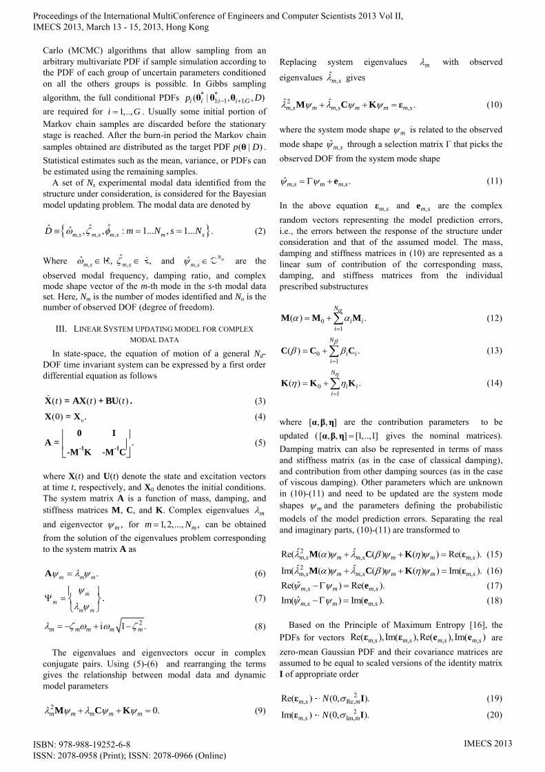
VII. ILLUSTRATIVE EXAMPLE The system selected for the illustrative example is a 4-

DOF mechanical system considered in [6] as shown in Fig. 1, and has the following properties: m1=m2=m3=m4=1 kg, k1=k3=k5=7000 N/m, k2=k4=8000 N/m, c1=c3=c5=0.7 N s/m, c2=c4=0.8 N s/m. The modal data for the model updating problem using Gibbs sampler for this system consists of 10 sets of modal data (Ns=10) with the first two modal frequencies, modal damping ratios, and partial complex mode shapes (corresponding to DOFs 1, 2, and 4, i.e., No=3) for each data set (Nm=2). Variability in modal data is introduced by perturbing the masses by 5%, and stiffnesses and dampings by 10%.

For Bayesian identification purpose, a dynamic model structure based on same 4-DOF mechanical system is considered and the uncertain parameters to be updated for this model class are contribution parameters 1 2 3 4[ , , , ] ,

1 2 3 4 5[ , , , , ] , 1 2 3 4 5[ , , , , ] , prediction error

variances 2 2 2 2Re,1 Im,1 Re,2 Im,2[ , , , ] , and complete complex

mode shapes 1 2[ , ] . Masses are assumed to be known with sufficient accuracy and thus the initial PDFs for

Proceedings of the International MultiConference of Engineers and Computer Scientists 2013 Vol II, IMECS 2013, March 13 - 15, 2013, Hong Kong

ISBN: 978-988-19252-6-8 ISSN: 2078-0958 (Print); ISSN: 2078-0966 (Online)

IMECS 2013

1 2 3 4[ , , , ] are chosen with mean values equal to 1 and coefficient of variation (c.o.v., i.e., the ratio of standard deviation to mean) for each equal to 1%; and prior mean values for 1 2 3 4 5[ , , , , ] and 1 2 3 4 5[ , , , , ] are assumed equal to 1, with prior c.o.v. for each equal to 20%. Flat independent priors are taken for 1 2[ , ] . Independent inverse gamma prior PDFs with 0 02, 0 are taken for

2 2 2 2Re,1 Im,1 Re,2 Im,2[ , , , ] (Jeffreys’ non-informative prior).

The total number of parameters to be updated is 34 (14 for the contribution parameters, 16 for the two mode shapes, and 4 prediction error variances).

Fig. 1. The 4-DOF mechanical system

Using the proposed Gibbs sampling based algorithm,

N=5,000 samples of contribution parameters, mode shapes and prediction errors variances are obtained. The burn-in period is less than 100 samples. Table I shows the statistical properties of the contribution parameters samples. It shows the estimated posterior mean values 1θ (column 2),

(a)

(b)

(c)

TABLE I BAYESIAN IDENTIFICATION RESULTS

Parameter Mean 1θ Standard Deviation

c.o.v. (%) 1 1| |

θ θ

m1 0.974 0.016 1.670 1.621

m2 0.982 0.031 3.150 0.600

m3 0.993 0.016 1.600 0.468

m4 1.009 0.039 3.880 0.226

c1 0.960 0.015 1.570 2.673

c2 0.959 0.020 2.050 2.101

c3 0.996 0.052 5.240 0.082

c4 0.992 0.020 2.050 0.385

c5 1.031 0.064 6.200 0.490

k1 1.013 0.021 2.060 0.641

k2 0.995 0.009 0.940 0.545

k3 0.995 0.010 0.990 0.561

k4 0.997 0.009 0.950 0.287

k5 0.997 0.010 0.990 0.290

m1

m2

m3

m4

c1 k1

c2 k2

c3 k3

c4 k4

c5 k5

Proceedings of the International MultiConference of Engineers and Computer Scientists 2013 Vol II, IMECS 2013, March 13 - 15, 2013, Hong Kong

ISBN: 978-988-19252-6-8 ISSN: 2078-0958 (Print); ISSN: 2078-0966 (Online)

IMECS 2013

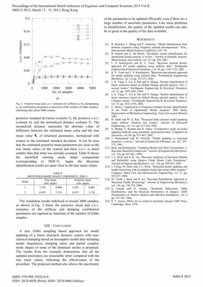
(d)

Fig. 2. Posterior mean and c.o.v. estimates for stiffness (a, b), and damping (c, d) contribution parameters as functions of the number of Gibbs samples, stabilizing after about 2000 samples. posterior standard deviation (column 3), the posterior c.o.v. (column 4), and the normalized distance (column 5). The normalized distance represents the absolute value of difference between the estimated mean value and the true mean value 1θ of structural parameters, normalized with respect to the estimated standard deviation. It can be seen that the estimated posterior mean parameters are close to the true mean values of the system and their c.o.v. is much smaller than that what was initially assumed. Table II shows the identified missing mode shape components (corresponding to DOF-3). Again the Bayesian identification results are quite close to the true mean values.

Table II IDENTIFIED MODE SHAPE COMPONENT, DOF-3

Mode True mean (abs, angle)

Posterior mean (abs, angle)

1 1.529 0.004 1.528 0.003

2 0.654 3.134 0.635 3.136

The simulation results stabilized at around 2000 samples,

as shown in Fig. 2 where the posterior mean and c.o.v. estimates of the stiffness and damping contribution parameters are reported as functions of the number of Gibbs samples.

VIII. CONCLUSION A new Gibbs sampling based approach for model

updating of a linear structural dynamic system with non-classical damping based on incomplete modal data including modal frequencies, damping ratios and partial complex mode shapes of some of the dominant modes is proposed. The results from the example demonstrate that all the updated parameters are reasonable when compared with the true mean values, indicating the effectiveness of the procedure. The proposed method also allows the uncertainty

of the parameters to be updated efficiently even if there are a large number of uncertain parameters. Like most problems in identification, the quality of the updated results can only be as good as the quality of the data available.

REFERENCES [1] R. Brincker, L. Zhang and P. Andersen, "Modal identification from

ambient responses using frequency domain decomposition," Proc.,

International Modal Analysis Conference, 625–30. [2] B. Peeters and G. De Roeck, "Stochastic system identification for

operational modal analysis: a review," Journal of Dynamic Systems,

Measurement, and Control, vol. 123, pp. 659, 2001. [3] L. S. Katafygiotis and K. V. Yuen, "Bayesian spectral density

approach for modal updating using ambient data," Earthquake

Engineering & Structural Dynamics, vol. 30, pp. 1103-1123, 2001. [4] K. V. Yuen and L. S. Katafygiotis, "Bayesian time-domain approach

for modal updating using ambient data," Probabilistic Engineering

Mechanics, vol. 16, pp. 219-231, 2001. [5] J. N. Yang, Y. Lei, S. Pan and N. Huang, "System identification of

linear structures based on Hilbert–Huang spectral analysis. Part 1: normal modes," Earthquake Engineering & Structural Dynamics, vol. 32, pp. 1443-1467, 2003.

[6] J. N. Yang, Y. Lei, S. Pan and N. Huang, "System identification of linear structures based on Hilbert–Huang spectral analysis. Part 2: Complex modes," Earthquake Engineering & Structural Dynamics, vol. 32, pp. 1533-1554, 2003.

[7] E. Parloo, "Application of Frequency-domain System Identification in the Field of Operational Modal Analysis," PhD thesis, Departement of Mechanical Engineering, Vrije Universiteit Brussel, 2003.

[8] B. Jaishi and W. X. Ren, "Structural finite element model updating using ambient vibration test results," Journal of Structural

Engineering, vol. 131, pp. 617-628, 2005. [9] S. Modak, T. Kundra and B. Nakra, "Comparative study of model

updating methods using simulated experimental data," Computers &

structures, vol. 80, pp. 437-447, 2002. [10] J. Mottershead and M. Friswell, "Model updating in structural

dynamics: a survey," Journal of Sound and Vibration, vol. 167, 347-375, 1993.

[11] Beck and Katafygiotis, "Updating Models and Their Uncertainties. I: Bayesian Statistical Framework," Journal of Engineering Mechanics, vol. 124, pp. 455-461, 1998.

[12] J. L. Beck and S. K. Au, "Bayesian Updating of Structural Models and Reliability using Markov Chain Monte Carlo Simulation," Journal of Engineering Mechanics, vol. 128, pp. 380-391, 2002.

[13] J. Ching, M. Muto and J. L. Beck, "Structural model updating and health monitoring with incomplete modal data using Gibbs sampler," Computer Aided Civil and Infrastructure Engineering, vol. 21, pp. 242-257, 2006.

[14] M. Vanik, J. Beck and S. Au, "Bayesian Probabilistic Approach to Structural Health Monitoring," Journal of Engineering Mechanics, vol. 126, pp. 738-745, 2000.

[15] S. Geman and D. Geman, "Stochastic Relaxation, Gibbs Distributions, and the Bayesian Restoration of Images," IEEE Transactions on Pattern Analysis and Machine Intelligence, vol. 6 pp. 721-741, 1984.

[16] E. T. Jaynes, Where do we stand on maximum entropy? MIT Press, Cambridge, Mass, 1978.

Proceedings of the International MultiConference of Engineers and Computer Scientists 2013 Vol II, IMECS 2013, March 13 - 15, 2013, Hong Kong

ISBN: 978-988-19252-6-8 ISSN: 2078-0958 (Print); ISSN: 2078-0966 (Online)

IMECS 2013