HE Plots for Repeated Measures Designs

Michael Friendly

York University, Toronto

Abstract

Hypothesis Error (HE) plots, introduced in Friendly (2007), provide graphical meth-ods to visualize hypothesis tests in multivariate linear models, by displaying hypothesisand error covariation as ellipsoids and providing visual representations of effect size andsignificance. These methods are implemented in the heplots package for R (Fox, Friendly,and Monette 2007) and SAS (Friendly 2006), and apply generally to designs with fixed-effect factors (MANOVA), quantitative regressors (multivariate multiple regression) andcombined cases (MANCOVA).

This paper describes the extension of these methods to repeated measures designs inwhich the multivariate responses represent the outcomes on one or more “within-subject”factors. This extension is illustrated using the heplots package for R. Examples describeone-sample profile analysis, designs with multiple between-S and within-S factors, anddoubly-multivariate designs, with multivariate responses observed on multiple occasions.

Keywords: data ellipse, HE plot, HE plot matrix, profile analysis, repeated measures, MANOVA,doubly-multivariate designs, mixed models.

1. Introduction

Hypothesis Error (HE) plots, introduced in Friendly (2007), provide graphical methods tovisualize hypothesis tests in multivariate linear models, by displaying hypothesis and error co-variation as ellipsoids and providing visual representations of effect size and significance. Theheplots package (Fox et al. 2007) for R (R Development Core Team 2010) implements thesemethods for the general class of the multivariate linear model (MVLM) including fixed-effectfactors (MANOVA), quantitative regressors (multivariate multiple regression (MMREG)) andcombined cases (MANCOVA). Here, we describe the extension of these methods to repeatedmeasures designs in which the multivariate responses represent the outcomes on one or more“within-subject” factors. This vignette also appears in the Journal of Statistical Software

(Friendly 2010).

1.1. Multivariate linear models: Notation

To set notation, we express the MVLM as

Y(n×p)

= X(n×q)

B(q×p)

+ U(n×p)

, (1)

where, Y ≡ (y1,y2, . . . ,yp) is the matrix of responses for n subjects on p variables, X isthe design matrix for q regressors, B is the q × p matrix of regression coefficients or model

2 HE Plots for Repeated Measures Designs

parameters and U is the n× p matrix of errors, with vec(U) ∼ Np(0, In⊗Σ), where ⊗ is theKronecker product.

A convenient feature of the MVLM for general multivariate responses is that all tests of linearhypotheses (for null effects) can be represented in the form of a general linear test,

H0 : L(h×q)

B(q×p)

= 0(h×p)

, (2)

where L is a matrix of constants whose rows specify h linear combinations or contrasts ofthe parameters to be tested simultaneously by a multivariate test. In R all such tests can becarried out using the functions Anova() and linearHypothesis() in the car package.1

For any such hypothesis of the form Eqn. (2), the analogs of the univariate sums of squaresfor hypothesis (SSH) and error (SSE) are the p× p sum of squares and crossproducts (SSP)matrices given by (Timm 1975, Ch. 3,5):

H ≡ SSPH = (LB)T [L(XTX)−LT]−1 (LB) , (3)

and

E ≡ SSPE = Y TY − BT(XTX)B = UTU , (4)

where U = Y −XB is the matrix of residuals. Multivariate test statistics (Wilks’ Λ, Pillaitrace, Hotelling-Lawley trace, Roy’s maximum root) for testing Eqn. (2) are based on thes = min(p, h) non-zero latent roots of HE−1 and attempt to capture how “large” H is,relative to E in s dimensions. All of these statistics have transformations to F statisticsgiving either exact or approximate null hypothesis F distributions. The corresponding latentvectors give a set of s orthogonal linear combinations of the responses that produce maximalunivariate F statistics for the hypothesis in Eqn. (2); we refer to these as the canonicaldiscriminant dimensions.

In a univariate, fixed-effects linear model, it is common to provide F tests for each term inthe model, summarized in an analysis-of-variance (ANOVA) table. The hypothesis sums ofsquares, SSH , for these tests can be expressed as differences in the error sums of squares, SSE ,for nested models. For example, dropping each term in the model in turn and contrastingthe resulting residual sum of squares with that for the full model produces so-called Type-IIItests; adding terms to the model sequentially produces so-called Type-I tests; and testing eachterm after all terms in the model with the exception of those to which it is marginal producesso-called Type-II tests. Closely analogous MANOVA tables can be formed similarly by takingdifferences in error sum of squares and products matrices (E) for such nested models. Type Itests are sensible only in special circumstances; in balanced designs, Type II and Type III testsare equivalent. Regardless, the methods illustrated in this paper apply to any multivariatelinear hypothesis.

1.2. Data ellipses and ellipsoids

In what follows, we make extensive use of ellipses (or ellipsoids in 3+D) to represent jointvariation among two or more variables, so we define this here. The data ellipse (or covariance

1 Both the car package and the heplots package are being actively developed. Except where noted, all resultsin this paper were produced using the old-stable versions on CRAN, car 1.2-16 (2009/10/10) and heplots

0.8-11 (2009-12-08) running under R version 3.4.1 (2017-06-30).

Michael Friendly 3

ellipse), described by Dempster (1969) and Monette (1990), is a device for visualizing therelationship between two variables, Y1 and Y2. Let D2

M (y) = (y − y)TS−1(y − y) representthe squared Mahalanobis distance of the point y = (y1, y2)

T from the centroid of the datay = (Y 1, Y 2)

T. The data ellipse Ec of size c is the set of all points y with D2M (y) less than or

equal to c2:

Ec(y;S,y) ≡{y: (y − y)TS−1(y − y) ≤ c2

}(5)

Here, S =∑n

i=1(y − y)T(y − y)/(n− 1) = Var(y) is the sample covariance matrix.

Many properties of the data ellipse hold regardless of the joint distribution of the variables, butif the variables are bivariate normal, then the data ellipse represents a contour of constantdensity in their joint distribution. In this case, D2

M (y) has a large-sample χ2 distributionwith 2 degrees of freedom, and so, for example, taking c2 = χ2

2(0.95) = 5.99 ≈ 6 enclosesapproximately 95 percent of the data. Taking c2 = χ2

2(0.68) = 2.28 gives a bivariate analogof the univariate ±1 standard deviation interval, enclosing approximately 68% of the data.

The generalization of the data ellipse to more than two variables is immediate: ApplyingEquation 5 to y = (y1, y2, y3)

T, for example, produces a data ellipsoid in three dimensions.For pmultivariate-normal variables, selecting c2 = χ2

p(1−α) encloses approximately 100(1−α)percent of the data.2

1.3. HE plots

The essential idea behind HE plots is that any multivariate hypothesis test Eqn. (2) can berepresented visually by ellipses (or ellipsoids in 3D) which express the size of co-variationagainst a multivariate null hypothesis (H) relative to error covariation (E). The multivariatetests, based on the latent roots of HE−1, are thus translated directly to the sizes of the H

ellipses for various hypotheses, relative to the size of the E ellipse. Moreover, the shape andorientation of these ellipses show something more– the directions (linear combinations of theresponses) that lead to various effect sizes and significance.

In these plots, the E matrix is first scaled to a covariance matrix (E/dfe = Var(Ui)). Theellipse drawn (translated to the centroid y of the variables) is thus the data ellipse of theresiduals, reflecting the size and orientation of residual variation. In what follows (by default),we always show these as “standard” ellipses of 68% coverage. This scaling and translationalso allows the means for levels of the factors to be displayed in the same space, facilitatinginterpretation.

The ellipses for H reflect the size and orientation of covariation against the null hypothesis.They always proportional to the data ellipse of the fitted effects (predicted values) for a givenhypothesized term. In relation to the E ellipse, the H ellipses can be scaled to show eitherthe effect size or strength of evidence against H0 (significance).

For effect size scaling, each H is divided by dfe to conform to E. The resulting ellipses arethen exactly the data ellipses of the fitted values, and correspond visually to multivariateanalogs of univariate effect size measures (e.g., (y1 − y2)/s where s=within group standarddeviation). That is, the sizes of the H ellipses relative to that of the E reflect the (squared)differences and correlation of the factor means relative to error covariation.

2 Robust versions of data ellipses (e.g., based on minimum volume ellipsoid (MVE) or minimum covariancedeterminant (MCD) estimators of S) are also available, as are small-sample approximations to the enclosingc2 radii, but these refinements are outside the scope of this paper.

4 HE Plots for Repeated Measures Designs

For significance scaling, it turns out to be most visually convenient to use Roy’s largest roottest as the test criterion. In this case the H ellipse is scaled to H/(λαdfe) where λα is thecritical value of Roy’s statistic. Using this gives a simple visual test of H0: Roy’s test rejectsH0 at a given α level if and only if the corresponding α-level H ellipse extends anywhereoutside the E ellipse.3 Consequently, when the rank of H = min(p, h) ≤ 2, all significanteffects can be observed directly in 2D HE plots; when rank(H) = 3, some rotation of a 3Dplot will reveal each significant effect as extending somewhere outside the E ellipsoid.

In our R implementation, the basic plotting functions in the heplots package are heplot()and heplot3d() for mlm objects. These rely heavily on the Anova() and other functions fromthe car package (Fox 2009) for computation. For more than three response variables, allpairwise HE plots can be shown using a pairs() function for mlm objects. Alternatively, therelated candisc package (Friendly and Fox 2009) produces HE plots in canonical discriminantspace. This shows a low-rank 2D (or 3D) view of the effects for a given term in the spaceof maximum discrimination, based on the linear combinations of responses which producemaximally significant test statistics. See Friendly (2007); Fox, Friendly, and Monette (2009)for details and examples for between-S MANOVA designs, MMREG and MANCOVA models.

2. Repeated measures designs

The framework for the MVLM described above pertains to the situation in which the re-sponse vectors (rows, yT

i of Yn×p) are iid and the p responses are separate, not necessarilycommensurate variables observed on individual i.

In principle, the MVLM extends quite elegantly to repeated-measure (or within-subject) de-signs, in which the p responses per individual can represent the factorial combination of one ormore factors that structure the response variables in the same way that the between-individualdesign structures the observations. In the multivariate approach to repeated measure data,the same model Eqn. (1) applies, but hypotheses about between- and within-individual vari-ation are tested by an extended form of the general linear test Eqn. (2), which becomes

H0 : L(h×q)

B(q×p)

M(p×k)

= 0(h×k)

, (6)

where M is a matrix of constants whose columns specify k linear combinations or contrastsamong the responses, corresponding to a particular within-individual effect. In this case, theH and E matrices for testing Eqn. (6) become

H = (LBM)T [L(XTX)−LT]−1 (LBM) , (7)

andE = (Y M)T[I − (XTX)−XT] (Y M) . (8)

This may be easily seen to be just the ordinary MVLM applied to the transformed responsesY M which form the basis for a given within-individual effect. The idea for this approachto repeated measures through a transformation of the responses was first suggested by Hsu

3Other multivariate tests (Wilks’ Λ, Hotelling-Lawley trace, Pillai trace) also have geometric interpretationsin HE plots (e.g., Wilks’ Λ is the ratio of areas (volumes) of the H and E ellipses (ellipsoids)), but thesestatistics do not provide such simple visual comparisons. All HE plots shown in this paper use significancescaling, based on Roy’s test.

Michael Friendly 5

(1938) and is discussed further by Rencher (1995) and Timm (1980). In what follows, werefer to hypotheses pertaining to between-individual effects (specified by L) as “between-S”and hypotheses pertaining to within-individual effects (M) as “within-S.”

Between-S effect tested

M for Within-S effects Intercept L = LA L = LB L = LAB

M = M1 =

(1 1 1

)T

µ.. A B A:B

M = MC =

1 −1 0

0 1 −1

T

C A:C B:C A:B:C

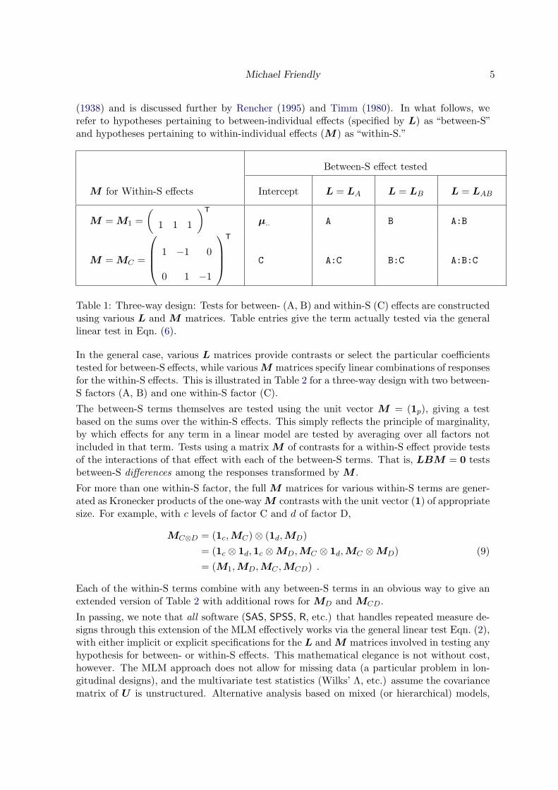
Table 1: Three-way design: Tests for between- (A, B) and within-S (C) effects are constructedusing various L and M matrices. Table entries give the term actually tested via the generallinear test in Eqn. (6).

In the general case, various L matrices provide contrasts or select the particular coefficientstested for between-S effects, while variousM matrices specify linear combinations of responsesfor the within-S effects. This is illustrated in Table 2 for a three-way design with two between-S factors (A, B) and one within-S factor (C).

The between-S terms themselves are tested using the unit vector M = (1p), giving a testbased on the sums over the within-S effects. This simply reflects the principle of marginality,by which effects for any term in a linear model are tested by averaging over all factors notincluded in that term. Tests using a matrix M of contrasts for a within-S effect provide testsof the interactions of that effect with each of the between-S terms. That is, LBM = 0 testsbetween-S differences among the responses transformed by M .

For more than one within-S factor, the full M matrices for various within-S terms are gener-ated as Kronecker products of the one-wayM contrasts with the unit vector (1) of appropriatesize. For example, with c levels of factor C and d of factor D,

MC⊗D = (1c,MC)⊗ (1d,MD)

= (1c ⊗ 1d,1c ⊗MD,MC ⊗ 1d,MC ⊗MD)

= (M1,MD,MC ,MCD) .

(9)

Each of the within-S terms combine with any between-S terms in an obvious way to give anextended version of Table 2 with additional rows for MD and MCD.

In passing, we note that all software (SAS, SPSS, R, etc.) that handles repeated measure de-signs through this extension of the MLM effectively works via the general linear test Eqn. (2),with either implicit or explicit specifications for the L and M matrices involved in testing anyhypothesis for between- or within-S effects. This mathematical elegance is not without cost,however. The MLM approach does not allow for missing data (a particular problem in lon-gitudinal designs), and the multivariate test statistics (Wilks’ Λ, etc.) assume the covariancematrix of U is unstructured. Alternative analysis based on mixed (or hierarchical) models,

6 HE Plots for Repeated Measures Designs

e.g. (Pinheiro and Bates 2000; Verbeke and Molenberghs 2000) are more general in someways, but to date visualization methods for this approach remain primitive and the mixedmodel analysis does not easily accommodate multivariate responses.

The remainder of the paper illustrates these MLM analyses, shows how they may be performedin R, and how HE plots can be used to provide visual displays of what is summarized in themultivariate test statistics. We freely admit that these displays are somewhat novel andtake some getting used to, and so this paper takes a more tutorial tone. We exemplify thesemethods in the context of simple, one-sample profile analysis (Section 3), designs with multiplebetween- and within-S effects (Section 4), and doubly-multivariate designs (Section 5), wheretwo or more separate responses (e.g., weight loss and self esteem) are each observed in afactorial structure over multiple within-S occasions. In Section 6 we describe a simplifiedinterface for these plots in the development versions of the heplots and car packages. Finally(Section 7) we compare these methods with visualizations based on the mixed model.

3. One sample profile analysis

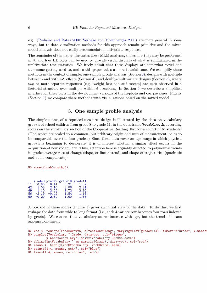
The simplest case of a repeated-measures design is illustrated by the data on vocabularygrowth of school children from grade 8 to grade 11, in the data frame VocabGrowth, recordingscores on the vocabulary section of the Cooperative Reading Test for a cohort of 64 students.(The scores are scaled to a common, but arbitrary origin and unit of measurement, so as tobe comparable over the four grades.) Since these data cover an age range in which physicalgrowth is beginning to decelerate, it is of interest whether a similar effect occurs in theacquisition of new vocabulary. Thus, attention here is arguably directed to polynomial trendsin grade: average rate of change (slope, or linear trend) and shape of trajectories (quadraticand cubic components).

R> some(VocabGrowth,5)

grade8 grade9 grade10 grade1111 -0.95 0.41 0.21 1.8242 1.03 2.10 3.88 2.8149 1.10 2.65 1.72 2.9656 -2.19 -0.42 1.54 1.1660 -0.29 2.62 1.60 1.86

A boxplot of these scores (Figure 1) gives an initial view of the data. To do this, we firstreshape the data from wide to long format (i.e., each 4-variate row becomes four rows indexedby grade). We can see that vocabulary scores increase with age, but the trend of meansappears non-linear.

R> voc <- reshape(VocabGrowth, direction="long", varying=list(grade=1:4), timevar="Grade", v.names=R> boxplot(Vocabulary ~ Grade, data=voc, col="bisque",

ylab="Vocabulary", main="Vocabulary Growth data")R> abline(lm(Vocabulary ~ as.numeric(Grade), data=voc), col="red")R> means <- tapply(voc$Vocabulary, voc$Grade, mean)R> points(1:4, means, pch=7, col="blue")R> lines(1:4, means, col="blue", lwd=2)

Michael Friendly 7

●

●

●

●

●

●

●

●

1 2 3 4

−2

02

46

810

Vocabulary Growth data

Voc

abul

ary

Figure 1: Boxplots of Vocabulary score by Grade, with linear regression line (red) and linesconnecting grade means (blue).

The standard univariate and multivariate tests for the differences in vocabulary with gradecan be carried out as follows. First, we fit the basic MVLM with an intercept only on theright-hand side of the model, since there are no between-S effects. The intercepts estimatethe means at each grade level, µ8, . . . , µ11.

R> (Vocab.mod <- lm(cbind(grade8,grade9,grade10,grade11) ~ 1, data=VocabGrowth))

Call:lm(formula = cbind(grade8, grade9, grade10, grade11) ~ 1, data = VocabGrowth)

Coefficients:grade8 grade9 grade10 grade11

(Intercept) 1.14 2.54 2.99 3.47

We could test the multivariate hypothesis that all means are simultaneously zero, µ8 = µ9 =µ10 = µ11 = 0. This point hypothesis is the simplest case of a multivariate test under Eqn. (2),with L = I.

R> (Vocab.aov0 <- Anova(Vocab.mod, type="III"))

Type III MANOVA Tests: Pillai test statisticDf test stat approx F num Df den Df Pr(>F)

(Intercept) 1 0.8577 90.38 4 60 <2e-16 ***---Signif. codes: 0 ✬***✬ 0.001 ✬**✬ 0.01 ✬*✬ 0.05 ✬.✬ 0.1 ✬ ✬ 1

8 HE Plots for Repeated Measures Designs

This hypothesis tests that the vocabulary means are all at the arbitrary origin for the scale.Often this test is not of direct interest, but it serves to illustrate the H and E matricesinvolved in any multivariate test, their representation by HE plots, and how we can extendthese plots to the repeated measures case.

The H and E matrices can be printed with summary(Vocab.aov0), or extracted from theAnova.mlm object. In this case, H is simply nyyT and E is the sum of squares and crossprod-ucts of deviations from the column means,

∑ni=1(yi − y)T(yi − y).

R> Vocab.aov0$SSP # H matrix

$❵(Intercept)❵grade8 grade9 grade10 grade11

grade8 82.810 185.037 217.547 252.525grade9 185.037 413.461 486.104 564.262grade10 217.547 486.104 571.509 663.398grade11 252.525 564.262 663.398 770.063

R> Vocab.aov0$SSPE # E matrix

grade8 grade9 grade10 grade11grade8 225.086 201.133 223.843 179.950grade9 201.133 273.850 223.515 191.729grade10 223.843 223.515 296.321 213.249grade11 179.950 191.729 213.249 233.848

The HE plot for the Vocab.mod model shows the test for the (Intercept) term (all means =0). To emphasize that the test is assessing the (squared) distance of y from 0, in relation tothe covariation of observations around the grand mean, we define a simple function to markthe point hypothesis H0 = (0, 0).

R> mark.H0 <- function(x=0, y=0, cex=2, pch=19, col="green3", lty=2, pos=2) {points(x,y, cex=cex, col=col, pch=pch)text(x,y, expression(H[0]), col=col, pos=pos)if (lty>0) abline(h=y, col=col, lty=lty)if (lty>0) abline(v=x, col=col, lty=lty)

}

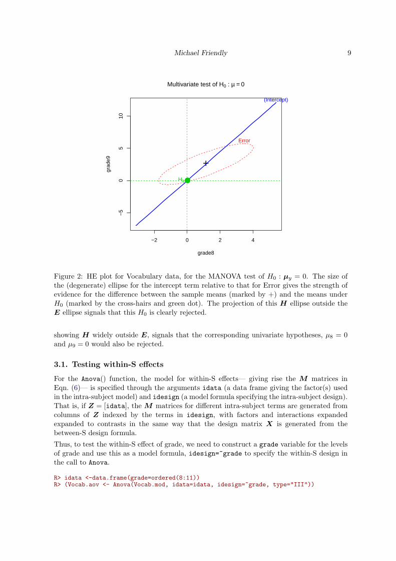
Here we show the HE plot for the grade8 and grade9 variables in Figure 2. The E ellipsereflects the positive correlation of vocabulary scores across these two grades, but also showsthat variability is greater in Grade 8 than in Grade 9. Its position relative to (0,0) indicatesthat both means are positive, with a larger mean at Grade 9 than Grade 8.

R> heplot(Vocab.mod, terms="(Intercept)", type="III")R> mark.H0(0,0)R> title(expression(paste("Multivariate test of ", H[0], " : ", bold(mu)==0)))

The H ellipse plots as a degenerate line because the H matrix has rank 1 (1 df for theMANOVA test of the Intercept). The fact that the H ellipse extends outside the E ellipse(anywhere) signals that this H0 is clearly rejected (for some linear combination of the responsevariables). Moreover, the projections of the H and E ellipses on the grade8 and grade9 axes,

Michael Friendly 9

−2 0 2 4

−5

05

10

grade8

grad

e9 +

Error

(Intercept)

●H0

Multivariate test of H0 : µ = 0

Figure 2: HE plot for Vocabulary data, for the MANOVA test of H0 : µy = 0. The size ofthe (degenerate) ellipse for the intercept term relative to that for Error gives the strength ofevidence for the difference between the sample means (marked by +) and the means underH0 (marked by the cross-hairs and green dot). The projection of this H ellipse outside theE ellipse signals that this H0 is clearly rejected.

showing H widely outside E, signals that the corresponding univariate hypotheses, µ8 = 0and µ9 = 0 would also be rejected.

3.1. Testing within-S effects

For the Anova() function, the model for within-S effects— giving rise the M matrices inEqn. (6)— is specified through the arguments idata (a data frame giving the factor(s) usedin the intra-subject model) and idesign (a model formula specifying the intra-subject design).That is, if Z = [idata], the M matrices for different intra-subject terms are generated fromcolumns of Z indexed by the terms in idesign, with factors and interactions expandedexpanded to contrasts in the same way that the design matrix X is generated from thebetween-S design formula.

Thus, to test the within-S effect of grade, we need to construct a grade variable for the levelsof grade and use this as a model formula, idesign=~grade to specify the within-S design inthe call to Anova.

R> idata <-data.frame(grade=ordered(8:11))R> (Vocab.aov <- Anova(Vocab.mod, idata=idata, idesign=~grade, type="III"))

10 HE Plots for Repeated Measures Designs

Type III Repeated Measures MANOVA Tests: Pillai test statisticDf test stat approx F num Df den Df Pr(>F)

(Intercept) 1 0.6529 118.50 1 63 4.12e-16 ***grade 1 0.8258 96.38 3 61 < 2e-16 ***---Signif. codes: 0 ✬***✬ 0.001 ✬**✬ 0.01 ✬*✬ 0.05 ✬.✬ 0.1 ✬ ✬ 1

As shown in Table 2, any such within-S test is effectively carried out using a transformationY to Y M , where the columns of M provide contrasts among the grades. For the overall

test of grade, any set of 3 linearly independent contrasts will give the same test statistics,though, of course the interpretation of the parameters will differ. Specifying grade as anordered factor (grade=ordered(8:11)) will cause Anova() to use the polynomial contrastsshown in Mpoly below.

Mpoly =

−3 1 −1−1 −1 31 −1 −33 1 1

Mfirst =

−1 −1 −11 0 00 1 00 0 1

Mlast =

1 0 00 1 00 0 1

−1 −1 −1

Alternatively,Mfirst would test the gains in vocabulary between grade 8 (baseline) and each ofgrades 9–11, while Mlast would test the difference between each of grades 8–10 from grade 11.(In R, these contrasts are constructed with M.first <- contr.sum(factor(11:8))[4:1,3:1],and M.last <- contr.sum(factor(8:11)) respectively.) In all cases, the hypothesis of nodifference among the means across grade is transformed to an equivalent multivariate pointhypothesis, Mµy = 0, such as we visualized in Figure 2.

Correspondingly, the HE plot for the effect of grade can be constructed as follows. Forexpository purposes we explicitly transform Y to Y M , where the columns of M providecontrasts among the grades reflecting linear, quadratic and cubic trends using Mpoly.

Using Mpoly, the MANOVA test for the grade effect is then testing H0 : Mµy = 0 ↔ µLin =µQuad = µCubic = 0. That is, the means across grades 8–11 are equal if and only if theirlinear, quadratic and cubic trends are simultaneously zero.

R> trends <- as.matrix(VocabGrowth) %*% poly(8:11, degree=3)R> colnames(trends)<- c("Linear", "Quad", "Cubic")R> # test all trend means = 0 == Grade effectR> within.mod <- lm(trends ~ 1)R> Anova(within.mod, type="III")

Type III MANOVA Tests: Pillai test statisticDf test stat approx F num Df den Df Pr(>F)

(Intercept) 1 0.8258 96.38 3 61 <2e-16 ***---Signif. codes: 0 ✬***✬ 0.001 ✬**✬ 0.01 ✬*✬ 0.05 ✬.✬ 0.1 ✬ ✬ 1

It is easily seen that the test of the (Intercept) term in within.mod is identical to the testof grade in Vocab.mod at the beginning of this subsection.

We can show this test visually as follows. Figure 3(a) shows a scatterplot of the transformedlinear and quadratic trend scores, overlayed with a 68% data ellipse. Figure 3(b) is thecorresponding HE plot for these two variables. Thus, we can see that theE ellipse is simply thedata ellipse of the transformed vocabulary scores; its orientation indicates a slight tendencyfor those with greater slopes (gain in vocabulary) to have greater curvatures (leveling offearlier). Figure 3 is produced as follows:

Michael Friendly 11

R> op <- par(mfrow=c(1,2))R> data.ellipse(trends[,1:2], xlim=c(-4,8), ylim=c(-3,3), levels=0.68,

main="(a) Data ellipse ")R> mark.H0(0,0)R> heplot(within.mod, terms="(Intercept)", col=c("red", "blue"), type="III",

term.labels="Grade", , xlim=c(-4,8), ylim=c(-3,3),main="(b) HE plot for Grade effect")

R> mark.H0(0,0)R> par(op)

−4 −2 0 2 4 6 8

−3

−2

−1

01

23

(a) Data ellipse

Linear

Qua

d

●●

●

●

●●

●

●

●

●

●

●

● ●

●

●

●

●

●●

●

●●

●

●

●

●

●

●

●

●

●

●

●

●

●

●

●

●

●

●

●

●

●

●

● ●

●

●

●

●

●

●●

●

●

●

●

●

●

●

●

●

●

●

●H0

−4 −2 0 2 4 6 8

−3

−2

−1

01

23

(b) HE plot for Grade effect

Linear

Qua

d

+

Error

Grade

●H0

Figure 3: Plots of linear and quadratic trend scores for the Vocabulary data. (a) Scatterplotwith 68% data ellipse; (b) HE plot for the effect of Grade. As in Figure 2, the size of the H

ellipse for Grade relative to the E ellipse shows the strength of evidence against H0.

We interpret Figure 3(b) as follows, bearing in mind that we are looking at the data in thetransformed space (Y M) of the linear (slopes) and quadratic (curvatures) of the originaldata (Y ). The mean slope is positive while the mean quadratic trend is negative. That is,overall, vocabulary increases with Grade, but at a decreasing rate. The H ellipse plots as adegenerate line because the H matrix has rank 1 (1 df for the MANOVA test of the Intercept).Its projection outside the E ellipse shows a highly significant rejection of the hypothesis ofequal means over Grade.

In such simple cases, traditional plots (boxplots, or plots of means with error bars) are easierto interpret. HE plots gain advantages in more complex designs (two or more between- orwithin-S factors, multiple responses), where they provide visual summaries of the informationused in the multivariate hypothesis tests.

4. Between- and within-S effects

When there are both within- and between-S effects, the multivariate and univariate hypothesestests can all be obtained together using Anova() with the idata and idesign specifying thewithin-S levels and the within-S design, as shown above. linearHypothesis() can be usedto test arbitrary contrasts in the within- or between- effects.

12 HE Plots for Repeated Measures Designs

However, to explain the visualization of these tests for within-S effects and their interactionsusing heplot() and related methods it is again convenient to explicitly transform Y 7→ Y M

for a given set of within-S contrasts, in the same way as done for the VocabGrowth data. SeeSection 6 for simplified code producing these HE plots directly, without the need for explicittransformation.

To illustrate, we use the data from O’Brien and Kaiser (1985) contained in the data frameOBrienKaiser in the car package. The data are from an imaginary study in which 16 femaleand male subjects, who are divided into three treatments, are measured at a pretest, posttest,and a follow-up session; during each session, they are measured at five occasions at intervalsof one hour. The design, therefore, has two between-subject and two within-subject factors.

For simplicity here, we initially collapse over the five occasions, and consider just the within-Seffect of session, called session in the analysis below.

R> library("car") # for OBrienKaiser dataR> # simplified analysis of OBrienKaiser data, collapsing over hourR> OBK <- OBrienKaiserR> OBK$pre <- rowMeans(OBK[,3:7])R> OBK$post <- rowMeans(OBK[,8:12])R> OBK$fup <- rowMeans(OBK[,13:17])R> # remove separate hour scoresR> OBK <- OBK[,-(3:17)]

Note that the between-S design is unbalanced (so tests based on Type II sum of squares andcrossproducts are preferred, because they conform to the principle of marginality).

R> table(OBK$gender, OBK$treatment)

control A BF 2 2 4M 3 2 3

The factors gender and treatment were specified with the following contrasts, Lgender, andLtreatment, shown below. The contrasts for treatment are nested (Helmert) contrasts testinga comparison of the control group with the average of treatments A and B (treatment1) andthe difference between treatments A and B (treatment2).

R> contrasts(OBK$gender)

[,1]F 1M -1

R> contrasts(OBK$treatment)

[,1] [,2]control -2 0A 1 -1B 1 1

We first fit the general MANOVA model for the three repeated measures in relation to thebetween-S factors. As before, this just establishes the model for the between-S effects.

Michael Friendly 13

R> # MANOVA modelR> mod.OBK <- lm(cbind(pre, post, fup) ~ treatment*gender, data=OBK)R> mod.OBK

Call:lm(formula = cbind(pre, post, fup) ~ treatment * gender, data = OBK)

Coefficients:pre post fup

(Intercept) 4.4722 5.7361 6.2917treatment1 0.1111 0.8264 0.9792treatment2 -0.4167 0.0625 0.0208gender1 -0.4722 -0.6528 -0.7083treatment1:gender1 -0.3611 -0.5347 -0.1875treatment2:gender1 0.6667 0.8125 0.8542

If we regarded the repeated measure effect of session as equally spaced, we could simplyuse polynomial contrasts to examine linear (slope) and quadratic (curvature) effects of time.Here, it makes more sense to use profile contrasts, testing (post - pre) and (fup - post).

R> session <- ordered(c("pretest", "posttest", "followup"),levels=c("pretest", "posttest", "followup"))

R> contrasts(session) <- matrix(c(-1, 1, 0,0, -1, 1), ncol=2)

R> session

[1] pretest posttest followupattr(,"contrasts")

[,1] [,2]pretest -1 0posttest 1 -1followup 0 1Levels: pretest < posttest < followup

R> idata <- data.frame(session)

The multivariate tests for all between- and within- effects are then calculated as follows:

R> # Multivariate tests for repeated measuresR> aov.OBK <- Anova(mod.OBK, idata=idata, idesign=~session, test="Roy")R> aov.OBK

Type II Repeated Measures MANOVA Tests: Roy test statisticDf test stat approx F num Df den Df Pr(>F)

(Intercept) 1 31.83 318.3 1 10 6.53e-09 ***treatment 2 0.93 4.6 2 10 0.037687 *gender 1 0.26 2.6 1 10 0.140974treatment:gender 2 0.57 2.9 2 10 0.104469session 1 5.69 25.6 2 9 0.000193 ***treatment:session 2 2.13 10.7 2 10 0.003309 **gender:session 1 0.05 0.2 2 9 0.819997treatment:gender:session 2 0.42 2.1 2 10 0.175303---Signif. codes: 0 ✬***✬ 0.001 ✬**✬ 0.01 ✬*✬ 0.05 ✬.✬ 0.1 ✬ ✬ 1

14 HE Plots for Repeated Measures Designs

It is useful to point out here that the default print methods for Anova.mlm objects, as shownabove, gives an optimally compact summary for all between- and within-S effects, using agiven test statistic, yet all details and other test statistics are available using the summary

method.4 For example, using summary(aov.OBK) as shown below, we can display all themultivariate tests together with the H and E matrices, and/or all the univariate tests forthe traditional univariate mixed model, under the assumption of sphericity and with Geiser-Greenhouse and Huhyn-Feldt corrected F tests. To conserve space in this article the resultsare not shown here.

R> # All multivariate testsR> summary(aov.OBK, univariate=FALSE)R> # Univariate tests for repeated measuresR> summary(aov.OBK, multivariate=FALSE)

OK, now its time to understand the nature of these effects. Ordinarily, from a data-analyticpoint of view, I would show traditional plots of means and other measures (as in Figure 1)or their generalizations in effect plots (Fox 1987; Fox and Hong 2009). But I’m not going todo that here. Instead, I’d like for you to understand how HE plots provide a compact visualsummary of an MLM, mirroring the tabular presentation from Anova(mod.OBK) above, butwhich also reveals the nature of effects. Here, you have to bear in mind that between-S effectsare displayed most naturally in the space of the response variables, while within-S effects aremost easily seen in the contrast space of transformed responses (Y M).

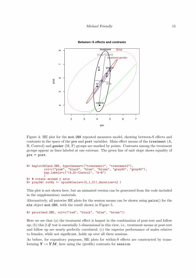
HE plots for between-S effects can be displayed for any pair of responses with heplot().Figure 4 shows this for pre and post. By default, H ellipses for all model terms (exclud-ing the intercept) are displayed. Additional MLM tests can also be displayed using thehypotheses argument; here we specify the two contrasts for the treatment effect shownabove as contrasts(OBK$treatment).

R> # HE plots for Between-S effectsR> heplot(mod.OBK, hypotheses=c("treatment1", "treatment2"),

col=c("red", "black", "blue", "brown", "gray40", "gray40"),hyp.labels=c("(A,B)-Control", "A-B"),main="Between-S effects and contrasts"

)R> lines(c(3,7), c(3,7), col="green")

In Figure 4, we see that the treatment effect is significant, and the large vertical extent ofthis H ellipse shows this is largely attributable to the differences among groups in the Postsession. Moreover, the main component of the treatment effect is the contrast between theControl group and groups A & B, which outperform the Control group at Post test. The effectof gender is not significant, but the HE plot shows that that males are higher than femalesat both Pre and Post tests. Likewise, the treatment:gender interaction fails significance,but the orientation of the H ellipse for this effect can be interpreted as showing that thedifferences among the treatment groups are larger for males than for females. Finally, theline of unit slope shows that for all effects, scores are greater on post than pre.

Using heplot3d(mod.OBK, ...) gives an interactive 3D version of Figure 4 for pre, post,and fup, that can be rotated and zoomed, or played as an animation.

4 In contrast, SAS proc glm and SPSS General Linear Model provide only more complete, but oftenbewildering outputs that still recall the days of Fortran coding in spite of more modern look and feel.

Michael Friendly 15

2 3 4 5 6 7

45

67

8

Between−S effects and contrasts

pre

post +

Errortreatment

gender

treatment:gender(A,B)−Control

A−B

●

●●

control

AB

●

●

F

M

Figure 4: HE plot for the mod.OBK repeated measures model, showing between-S effects andcontrasts in the space of the pre and post variables. Main effect means of the treatment (A,B, Control) and gender (M, F) groups are marked by points. Contrasts among the treatmentgroups appear as lines labeled at one extreme. The green line of unit slope shows equality ofpre = post.

R> heplot3d(mod.OBK, hypotheses=c("treatment1", "treatment2"),col=c("pink", "black", "blue", "brown", "gray40", "gray40"),hyp.labels=c("(A,B)-Control", "A-B"))

R> # rotate around y axisR> play3d( rot8y <- spin3d(axis=c(0,1,0)),duration=12 )

This plot is not shown here, but an animated version can be generated from the code includedin the supplementary materials.

Alternatively, all pairwise HE plots for the session means can be shown using pairs() for themlm object mod.OBK, with the result shown in Figure 5.

R> pairs(mod.OBK, col=c("red", "black", "blue", "brown"))

Here we see that (a) the treatment effect is largest in the combination of post-test and followup; (b) this 2 df test is essentially 1-dimensional in this view, i.e., treatment means at post-testand follow up are nearly perfectly correlated; (c) the superior performance of males relativeto females, while not significant, holds up over all three sessions.

As before, for expository purposes, HE plots for within-S effects are constructed by trans-forming Y 7→ Y M , here using the (profile) contrasts for session.

16 HE Plots for Repeated Measures Designs

pre

2

8

+

Error

treatmentgender

treatment:gender

●

●

●

control

A

B●

●

F

M

+

Error

treatmentgender

treatment:gender

●

●

●

control

A

B●

●

F

M

+

Errortreatment

gender

treatment:gender

●

●●

control

AB

●

●

F

M

post

3

9

+

Error treatment

gender

treatment:gender

●

●●

control

AB

●

●

F

M

+

Error

treatment

gendertreatment:gender

●

●●

control

AB

●

●

F

M

+

Error

treatment

gendertreatment:gender

●

●●

control

AB

●

●

F

M

fup

3

9

Figure 5: HE plot for the mod.OBK repeated measures model, showing between-S effects forall pairs of sessions. The panel in row 2, column 1 is identical to that shown separately inFigure 4.

R> # Transform to profile contrasts for within-S effectsR> OBK$session.1 <- OBK$post - OBK$preR> OBK$session.2 <- OBK$fup - OBK$postR> mod1.OBK <- lm(cbind(session.1, session.2) ~ treatment*gender, data=OBK)R> Anova(mod1.OBK, test="Roy", type="III")

Type III MANOVA Tests: Roy test statisticDf test stat approx F num Df den Df Pr(>F)

(Intercept) 1 4.366 19.645 2 9 0.000521 ***treatment 2 2.186 10.932 2 10 0.003044 **gender 1 0.071 0.319 2 9 0.734970treatment:gender 2 0.417 2.083 2 10 0.175303---Signif. codes: 0 ✬***✬ 0.001 ✬**✬ 0.01 ✬*✬ 0.05 ✬.✬ 0.1 ✬ ✬ 1

From the schematic summary in Table 2, with these (or any other) contrasts as Msession,the tests of the effects contained in treatment*gender in mod1.OBK are identical to theinteractions of these terms with session, as shown above for the full model in aov.OBK. The(Intercept) term in this model represents the session effect.

Michael Friendly 17

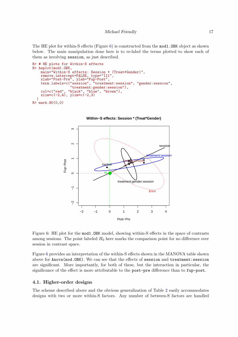
The HE plot for within-S effects (Figure 6) is constructed from the mod1.OBK object as shownbelow. The main manipulation done here is to re-label the terms plotted to show each ofthem as involving session, as just described.

R> # HE plots for Within-S effectsR> heplot(mod1.OBK,

main="Within-S effects: Session * (Treat*Gender)",remove.intercept=FALSE, type="III",xlab="Post-Pre", ylab="Fup-Post",term.labels=c("session", "treatment:session", "gender:session",

"treatment:gender:session"),col=c("red", "black", "blue", "brown"),xlim=c(-2,4), ylim=c(-2,3)

)R> mark.H0(0,0)

−2 −1 0 1 2 3 4

−2

−1

01

23

Within−S effects: Session * (Treat*Gender)

Post−Pre

Fup

−P

ost

+

Error

session

treatment:session

gender:session

treatment:gender:session

●

● ●control

A B●●

FM

●H0

Figure 6: HE plot for the mod1.OBK model, showing within-S effects in the space of contrastsamong sessions. The point labeled H0 here marks the comparison point for no difference oversession in contrast space.

Figure 6 provides an interpretation of the within-S effects shown in the MANOVA table shownabove for Anova(mod.OBK). We can see that the effects of session and treatment:session

are significant. More importantly, for both of these, but the interaction in particular, thesignificance of the effect is more attributable to the post-pre difference than to fup-post.

4.1. Higher-order designs

The scheme described above and the obvious generalization of Table 2 easily accommodatesdesigns with two or more within-S factors. Any number of between-S factors are handled

18 HE Plots for Repeated Measures Designs

automatically, by the model formula for between-S effects specified in the lm() call, e.g.,~ treatment * gender.

For example, for the O’Brien-Kaiser data with session and hour as two within-S factors, firstcreate a data frame, within specifying the values of these factors for the 3× 5 combinations.

R> session <- factor(rep(c("pretest", "posttest", "followup"), c(5, 5, 5)),levels=c("pretest", "posttest", "followup"))

R> contrasts(session) <- matrix(c(-1, 1, 0,0, -1, 1), ncol=2)

R> hour <- ordered(rep(1:5, 3))R> within <- data.frame(session, hour)

The within data frame looks like this:

R> str(within)

✬data.frame✬: 15 obs. of 2 variables:$ session: Factor w/ 3 levels "pretest","posttest",..: 1 1 1 1 1 2 2 2 2 2 .....- attr(*, "contrasts")= num [1:3, 1:2] -1 1 0 0 -1 1.. ..- attr(*, "dimnames")=List of 2.. .. ..$ : chr "pretest" "posttest" "followup".. .. ..$ : NULL$ hour : Ord.factor w/ 5 levels "1"<"2"<"3"<"4"<..: 1 2 3 4 5 1 2 3 4 5 ...

R> within

session hour1 pretest 12 pretest 23 pretest 34 pretest 45 pretest 56 posttest 17 posttest 28 posttest 39 posttest 410 posttest 511 followup 112 followup 213 followup 314 followup 415 followup 5

The repeated measures MANOVA analysis can then be carried out as follows:

R> mod.OBK2 <- lm(cbind(pre.1, pre.2, pre.3, pre.4, pre.5,post.1, post.2, post.3, post.4, post.5,fup.1, fup.2, fup.3, fup.4, fup.5) ~ treatment*gender,

data=OBrienKaiser)R> (aov.OBK2 <- Anova(mod.OBK2, idata=within, idesign=~session*hour, test="Roy"))

Type II Repeated Measures MANOVA Tests: Roy test statisticDf test stat approx F num Df den Df Pr(>F)

(Intercept) 1 31.83 318.3 1 10 6.53e-09 ***treatment 2 0.93 4.6 2 10 0.037687 *gender 1 0.26 2.6 1 10 0.140974treatment:gender 2 0.57 2.9 2 10 0.104469

Michael Friendly 19

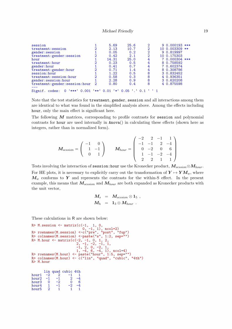
session 1 5.69 25.6 2 9 0.000193 ***treatment:session 2 2.13 10.7 2 10 0.003309 **gender:session 1 0.05 0.2 2 9 0.819997treatment:gender:session 2 0.42 2.1 2 10 0.175303hour 1 14.31 25.0 4 7 0.000304 ***treatment:hour 2 0.23 0.5 4 8 0.758592gender:hour 1 0.41 0.7 4 7 0.602374treatment:gender:hour 2 0.71 1.4 4 8 0.308786session:hour 1 1.22 0.5 8 3 0.832452treatment:session:hour 2 0.58 0.3 8 4 0.936351gender:session:hour 1 2.28 0.9 8 3 0.620208treatment:gender:session:hour 2 0.80 0.4 8 4 0.875598---Signif. codes: 0 ✬***✬ 0.001 ✬**✬ 0.01 ✬*✬ 0.05 ✬.✬ 0.1 ✬ ✬ 1

Note that the test statistics for treatment, gender, session and all interactions among themare identical to what was found in the simplified analysis above. Among the effects includinghour, only the main effect is significant here.

The following M matrices, corresponding to profile contrasts for session and polynomialcontrasts for hour are used internally in Anova() in calculating these effects (shown here asintegers, rather than in normalized form).

Msession =

−1 01 −10 1

Mhour =

−2 2 −1 1−1 −1 2 −40 −2 0 61 −1 −2 −42 2 1 1

Tests involving the interaction of session:hour use the Kronecker product, Msession⊗Mhour.

For HE plots, it is necessary to explicitly carry out the transformation of Y 7→ Y Mw, whereMw conforms to Y and represents the contrasts for the within-S effect. In the presentexample, this means that Msession and Mhour are both expanded as Kronecker products withthe unit vector,

Ms = Msession ⊗ 15 ,

Mh = 13 ⊗Mhour .

These calculations in R are shown below:

R> M.session <- matrix(c(-1, 1, 0,0, -1, 1), ncol=2)

R> rownames(M.session) <-c("pre", "post", "fup")R> colnames(M.session) <-paste("s", 1:2, sep="")R> M.hour <- matrix(c(-2, -1, 0, 1, 2,

2, -1, -2, -1, 1,-1, 2, 0, -2, 1,1, -4, 6, -4, 1), ncol=4)

R> rownames(M.hour) <- paste("hour", 1:5, sep="")R> colnames(M.hour) <- c("lin", "quad", "cubic", "4th")R> M.hour

lin quad cubic 4thhour1 -2 2 -1 1hour2 -1 -1 2 -4hour3 0 -2 0 6hour4 1 -1 -2 -4hour5 2 1 1 1

20 HE Plots for Repeated Measures Designs

R> unit <- function(n, prefix="") {J <-matrix(rep(1, n), ncol=1)rownames(J) <- paste(prefix, 1:n, sep="")J

}R> M.s <- kronecker( M.session, unit(5, "h"), make.dimnames=TRUE)R> (M.h <- kronecker( unit(3, "s"), M.hour, make.dimnames=TRUE))

:lin :quad :cubic :4ths1:hour1 -2 2 -1 1s1:hour2 -1 -1 2 -4s1:hour3 0 -2 0 6s1:hour4 1 -1 -2 -4s1:hour5 2 1 1 1s2:hour1 -2 2 -1 1s2:hour2 -1 -1 2 -4s2:hour3 0 -2 0 6s2:hour4 1 -1 -2 -4s2:hour5 2 1 1 1s3:hour1 -2 2 -1 1s3:hour2 -1 -1 2 -4s3:hour3 0 -2 0 6s3:hour4 1 -1 -2 -4s3:hour5 2 1 1 1

R> M.sh <- kronecker( M.session, M.hour, make.dimnames=TRUE)

Using M.h, we can construct the within-model for all terms involving the hour effect,

R> Y.hour <- as.matrix(OBrienKaiser[,3:17]) %*% M.hR> mod.OBK2.hour <- lm(Y.hour ~ treatment*gender, data=OBrienKaiser)

We can plot these effects for the linear and quadratic contrasts of hour, representing within-session slope and curvature. Figure 7 is produced as shown below. As shown by theAnova(mod.OBK2, ...) above, all interactions with hour are small, and so these appearwholly contained within the E ellipse. In particular, there are no differences among groups(treatment × gender) in the slopes or curvatures over hour. For the main effect of hour, thelinear effect is almost exactly zero, while the quadratic effect is huge.

R> labels <- c("hour", paste(c("treatment","gender","treatment:gender"),":hour", sep=""))R> colors <- c("red", "black", "blue", "brown", "purple")R> heplot(mod.OBK2.hour, type="III", remove.intercept=FALSE, term.labels=labels, col=colors)R> mark.H0()

The pairs() function shows these effects (Figure 8) for all contrasts in hour. To reduce clutter,we only label the hour effect, since all interactions with hour are small and non-significant.The main additional message here is that the effects of hour are more complex than just thelarge quadratic component we saw in Figure 7.

R> pairs(mod.OBK2.hour, type="III", remove.intercept=FALSE, term.labels="hour", col=colors)

5. Doubly-multivariate designs

Michael Friendly 21

−15 −10 −5 0 5 10 15

−60

−40

−20

0

:lin

:qua

d

+

Error

hour

treatment:hour

gender:hourtreatment:gender:hour●

●

●

control

AB

●●FM

●H0

Figure 7: HE plot for the mod.OBK2 repeated measures model, showing within-S effects forlinear and quadratic contrasts in hour. As in Figure 6, we are viewing hypothesis and errorvariation in the transformed space of the repeated measures contrasts, here given by Mh.

In the designs discussed above the same measure is observed on all occasions. Sometimes,there are two or more different measures, Y1, Y2, . . . , observed at each occasion, for exampleresponse speed and accuracy. In these cases, researchers often carry out separate repeatedmeasures analyses for each measure. However the tests of between-S effects and each within-Seffect can also be carried out as multivariate tests of Y1, Y2, . . . simultaneously, and these testsare often more powerful, particularly when the effects for the different measures are weak,but correlated.

In the present context, such doubly-multivariate designs can be easily handled in principle bytreating the multiple measures as an additional within-S factor, but using an identity matrixas the M matrix in forming the linear hypotheses to be tested via Eqn. (6). For example,with two measures, Y1, Y2 observed on three repeated sessions, the full M matrix for thedesign is generated as in Eqn. (9) as

MCM = (1,Msession)⊗ I2 =

1 −1 01 1 −11 0 1

⊗

(1 00 1

). (10)

In R, we can express this as follows, using M.measure to represent Y1, Y2.

R> M.measure <- diag(2)R> rownames(M.measure)<- c("Y1", "Y2")R> colnames(M.measure)<- c("Y1", "Y2")R> kronecker(cbind(1, M.session), M.measure, make.dimnames=TRUE)

22 HE Plots for Repeated Measures Designs

:lin

−15

16

+

Error

hour●

●●

controlAB●●

FM +

Error

hour●

●●

controlAB●

●

FM +

Error

hour●●

●

controlAB●

●

FM

+Error

hour

●

●●

controlAB●●FM :quad

−43

−19

+Error

hour

●

●●

controlAB

● ●F M +

Error

hour

●

●●

controlAB●●FM

+

Error

hour

●

●●controlAB

●

●

F

M

+

Error

hour

●

●●controlAB

●

●

F

M

:cubic

−12

4

+

Error

hour

●

●●controlAB

●

●

F

M

+

Errorhour

● ●●

controlAB

●●

FM +

Error hour

●●●

controlAB●●

FM +

Error

hour

● ●●

controlAB

● ●

F M:4th

−20

35

Figure 8: HE plot for the mod.OBK2 repeated measures model, showing within-S effects forall pairs of contrasts in hour.

:Y1 :Y2 s1:Y1 s1:Y2 s2:Y1 s2:Y2pre:Y1 1 0 -1 0 0 0pre:Y2 0 1 0 -1 0 0post:Y1 1 0 1 0 -1 0post:Y2 0 1 0 1 0 -1fup:Y1 1 0 0 0 1 0fup:Y2 0 1 0 0 0 1

In the result, the first two columns correspond to the within-S Intercept term, and are usedto test all between-S terms for Y1, Y2 simultaneously. The remaining columns correspond tothe session effect for both variables and all interactions with session. In practice, this analysismust be performed in stages because Anova() does not (yet)5 allow such a doubly-multivariatedesign to be specified directly.

5.1. Example: Weight loss and self esteem

To illustrate, we consider the data frame WeightLoss originally from Andrew Ainsworth(http://www.csun.edu/~ata20315/psy524/main.htm), giving (contrived) data on weightloss and measures of self esteem after each of three months for 34 individuals, who wereobserved in one of three groups: Control, Diet group, Diet + Exercise group. The within-Sfactors are thus measure (wl, se) and month (1:3).

R> table(WeightLoss$group)

5The new version of the car package (2.0-0) on CRAN now includes enhanced Anova() andlinearHypothesis() which perform these analyses.

Michael Friendly 23

Control Diet DietEx12 12 10

R> some(WeightLoss)

group wl1 wl2 wl3 se1 se2 se36 Control 6 5 4 17 18 1811 Control 4 2 2 16 16 1112 Control 5 2 1 15 13 1619 Diet 4 3 1 12 11 1420 Diet 4 2 1 12 11 1121 Diet 6 5 3 17 16 1924 Diet 7 4 3 16 14 1828 DietEx 3 4 1 16 13 1729 DietEx 3 5 1 13 13 1630 DietEx 6 5 2 15 12 18

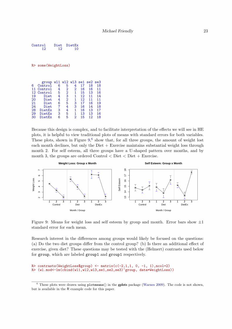
Because this design is complex, and to facilitate interpretation of the effects we will see in HEplots, it is helpful to view traditional plots of means with standard errors for both variables.These plots, shown in Figure 9,6 show that, for all three groups, the amount of weight losteach month declines, but only the Diet + Exercise maintains substantial weight loss throughmonth 2. For self esteem, all three groups have a U-shaped pattern over months, and bymonth 3, the groups are ordered Control < Diet < Diet + Exercise.

23

45

67

Weight Loss: Group x Month

Month / Group

Wei

ght L

oss

1 2Control

3 1 2Diet

3 1 2DietEx

3

1314

1516

1718

Self Esteem: Group x Month

Month / Group

Sel

f Est

eem

1 2Control

3 1 2Diet

3 1 2DietEx

3

Figure 9: Means for weight loss and self esteem by group and month. Error bars show ±1standard error for each mean.

Research interest in the differences among groups would likely be focused on the questions:(a) Do the two diet groups differ from the control group? (b) Is there an additional effect ofexercise, given diet? These questions may be tested with the (Helmert) contrasts used belowfor group, which are labeled group1 and group1 respectively.

R> contrasts(WeightLoss$group) <- matrix(c(-2,1,1, 0, -1, 1),ncol=2)R> (wl.mod<-lm(cbind(wl1,wl2,wl3,se1,se2,se3)~group, data=WeightLoss))

6 These plots were drawn using plotmeans() in the gplots package (Warnes 2009). The code is not shown,but is available in the R example code for this paper.

24 HE Plots for Repeated Measures Designs

Call:lm(formula = cbind(wl1, wl2, wl3, se1, se2, se3) ~ group, data = WeightLoss)

Coefficients:wl1 wl2 wl3 se1 se2 se3

(Intercept) 5.3444 4.4500 2.1778 14.9278 13.7944 16.2833group1 0.4222 0.5583 0.0472 0.0889 -0.2694 0.6000group2 0.4333 1.0917 -0.0250 0.1833 -0.2250 0.7167

A standard between-S MANOVA, ignoring the within-S structure shows a highly significantgroup effect.

R> Anova(wl.mod)

Type II MANOVA Tests: Pillai test statisticDf test stat approx F num Df den Df Pr(>F)

group 2 0.7255 2.562 12 54 0.00924 **---Signif. codes: 0 ✬***✬ 0.001 ✬**✬ 0.01 ✬*✬ 0.05 ✬.✬ 0.1 ✬ ✬ 1

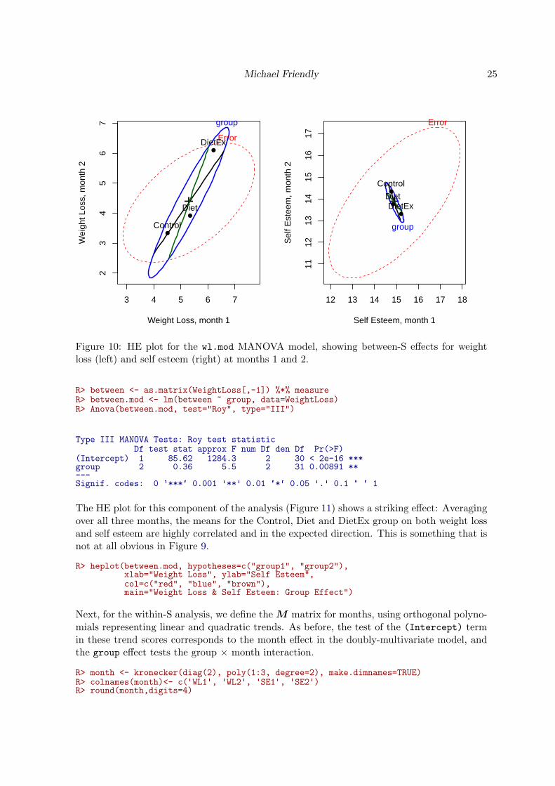
As before, it is often useful to examine HE plots for pairs of variables in this analysis beforeproceeding to the within-S analysis. For example, Figure 10 shows the test of group and thetwo contrasts for weight loss and for self esteem at months 1 and 2.

R> op <- par(mfrow=c(1,2))R> heplot(wl.mod, hypotheses=c("group1", "group2"),

xlab="Weight Loss, month 1", ylab="Weight Loss, month 2")R> heplot(wl.mod, hypotheses=c("group1", "group2"), variables=4:5,

xlab="Self Esteem, month 1", ylab="Self Esteem, month 2")R> par(op)

This is helpful, but doesn’t illuminate the overall group effect for weight loss and self esteemfor all three months, and, of course cannot shed light on any interactions of group with measureor month. In the following discussion, we will assume that the researcher is particularlyinterested in understanding the relation between weight loss and self esteem as it is expressedin changes over time and differences among groups.

To carry out the doubly-multivariate analysis, we proceed as follows. First, we define the M

matrix for the measures, used in the between-S analysis. We use M = I2 ⊗ 1/3 so that theresulting scores are the means (not sums) for weight loss and self esteem.

R> measure <- kronecker(diag(2), unit(3, ✬M✬)/3, make.dimnames=TRUE)R> colnames(measure)<- c(✬WL✬, ✬SE✬)R> measure

WL SE:M1 0.333333 0.000000:M2 0.333333 0.000000:M3 0.333333 0.000000:M1 0.000000 0.333333:M2 0.000000 0.333333:M3 0.000000 0.333333

Michael Friendly 25

3 4 5 6 7

23

45

67

Weight Loss, month 1

Wei

ght L

oss,

mon

th 2

+

Error

group

●

●

●

Control

Diet

DietEx

12 13 14 15 16 17 1811

1213

1415

1617

Self Esteem, month 1

Sel

f Est

eem

, mon

th 2

+

Error

group

●

●

●

Control

DietDietEx

Figure 10: HE plot for the wl.mod MANOVA model, showing between-S effects for weightloss (left) and self esteem (right) at months 1 and 2.

R> between <- as.matrix(WeightLoss[,-1]) %*% measureR> between.mod <- lm(between ~ group, data=WeightLoss)R> Anova(between.mod, test="Roy", type="III")

Type III MANOVA Tests: Roy test statisticDf test stat approx F num Df den Df Pr(>F)

(Intercept) 1 85.62 1284.3 2 30 < 2e-16 ***group 2 0.36 5.5 2 31 0.00891 **---Signif. codes: 0 ✬***✬ 0.001 ✬**✬ 0.01 ✬*✬ 0.05 ✬.✬ 0.1 ✬ ✬ 1

The HE plot for this component of the analysis (Figure 11) shows a striking effect: Averagingover all three months, the means for the Control, Diet and DietEx group on both weight lossand self esteem are highly correlated and in the expected direction. This is something that isnot at all obvious in Figure 9.

R> heplot(between.mod, hypotheses=c("group1", "group2"),xlab="Weight Loss", ylab="Self Esteem",col=c("red", "blue", "brown"),main="Weight Loss & Self Esteem: Group Effect")

Next, for the within-S analysis, we define the M matrix for months, using orthogonal polyno-mials representing linear and quadratic trends. As before, the test of the (Intercept) termin these trend scores corresponds to the month effect in the doubly-multivariate model, andthe group effect tests the group × month interaction.

R> month <- kronecker(diag(2), poly(1:3, degree=2), make.dimnames=TRUE)R> colnames(month)<- c(✬WL1✬, ✬WL2✬, ✬SE1✬, ✬SE2✬)R> round(month,digits=4)

26 HE Plots for Repeated Measures Designs

2 3 4 5 6

1314

1516

17

Weight Loss & Self Esteem: Group Effect

Weight Loss

Sel

f Est

eem

+

Error

group

●

●

●

ControlDiet

DietEx

Figure 11: HE plot for the between.mod doubly-multivariate design, showing overall between-S effects for weight loss and self esteem.

WL1 WL2 SE1 SE2: -0.7071 0.4082 0.0000 0.0000: 0.0000 -0.8165 0.0000 0.0000: 0.7071 0.4082 0.0000 0.0000: 0.0000 0.0000 -0.7071 0.4082: 0.0000 0.0000 0.0000 -0.8165: 0.0000 0.0000 0.7071 0.4082

R> trends <- as.matrix(WeightLoss[,-1]) %*% monthR> within.mod <- lm(trends ~ group, data=WeightLoss)R> Anova(within.mod, test="Roy", type="III")

Type III MANOVA Tests: Roy test statisticDf test stat approx F num Df den Df Pr(>F)

(Intercept) 1 9.928 69.50 4 28 3.96e-14 ***group 2 1.772 12.84 4 29 3.91e-06 ***---Signif. codes: 0 ✬***✬ 0.001 ✬**✬ 0.01 ✬*✬ 0.05 ✬.✬ 0.1 ✬ ✬ 1

HE plots corresponding to this model (Figure 12) can be produced as follows. The H and E

matrices are all 4× 4, but the H matrices for the month and group:month effects are rank 1and 2 respectively.

R> op <- par(mfrow=c(1,2))R> heplot(within.mod, hypotheses=c("group1", "group2"), variables=c(1,3),

xlab="Weight Loss - Linear", ylab="Self Esteem - Linear",type="III", remove.intercept=FALSE,

Michael Friendly 27

term.labels=c("month", "group:month"),main="(a) Within-S Linear Effects")

R> mark.H0()R> heplot(within.mod, hypotheses=c("group1", "group2"), variables=c(2,4),

xlab="Weight Loss - Quadratic", ylab="Self Esteem - Quadratic",type="III", remove.intercept=FALSE,term.labels=c("month", "group:month"),main="(b) Within-S Quadratic Effects")

R> mark.H0()R> par(op)

−8 −6 −4 −2 0 2 4

−1

01

23

(a) Within−S Linear Effects

Weight Loss − Linear

Sel

f Est

eem

− L

inea

r

+

Error

month

group:month

●

●

●

Control

Diet

DietEx

●H0

−2.0 −1.5 −1.0 −0.5 0.0 0.5 1.0

−2

02

4

(b) Within−S Quadratic Effects

Weight Loss − Quadratic

Sel

f Est

eem

− Q

uadr

atic

+

Error

month

group:month

●

●

●

Control

Diet

DietEx

●H0

Figure 12: HE plots for the within.mod doubly-multivariate design, showing the effects ofmonth and the interaction group:month for weight loss vs. self esteem. (a) Linear effects; (b)Quadratic effects.

Figure 12 shows the plots for the linear and quadratic effects separately for weight loss vs.self esteem. The plot of linear effects (Figure 12(a)) shows that the effect of month can bebe described as negative slopes for weight loss combined with positive slopes for self esteem–all groups lose progressively less weight over time, but generally feel better about themselves.Differences among groups in the group:month effect are in the same direction, but with greaterdifferences among groups in the slopes for self esteem. The interpretation of the quadraticeffects (Figure 12(b)) is similar, except here, differences in curvature over months are drivenlargely by the difference between the DietEx group from the others on weight loss.

The interested reader might wish to compare the standard univariate plots of means in Fig-ure 9 with the HE plots in Figure 11 and Figure 12. The univariate plots have the advantageof showing the data directly, but cannot show the sources of significant effects in multivariaterepeated measures models. HE plots have the advantage that they show directly what isexpressed in the multivariate tests for relevant hypotheses.

6. Simplified interface: heplots 0.9 and car 2.0

It sometimes happens that the act of describing and illustrating software spurs developmentto make both simpler, and such is the case here. At the beginning, the stable version of car on

28 HE Plots for Repeated Measures Designs

CRAN provided the computation for multivariate linear hypotheses including repeated mea-sures designs, but could not handle doubly-multivariate designs directly; the CRAN versionof heplots could only repeated measures by explicitly transforming Y 7→ Y M and re-fittingsubmodels in terms of the transformed responses.

The new versions of these packages on CRAN (http://cran.us.r-project.org/) now han-dle these cases directly from the basic mlm object. heplot() now provides the argumentsidata, idesign, icontrasts, or, for the doubly-multivariate case, imatrix, which are passedto Anova() to calculate the appropriate H and E matrices.

Omitting these arguments in the call to heplot() gives an HE plot for all between-S effects(or the subset specified by the terms argument), just as before. For the within-S effects, Ematrices differ for for different within-S terms, so it is necessary to specify the intra-subjectterm (iterm, corresponding to M) for which HE plots are desired. Several examples are givenbelow.

For the VocabularyGrowth data, Figure 3(b) can be produced by

R> (Vocab.mod <- lm(cbind(grade8,grade9,grade10,grade11) ~ 1, data=VocabGrowth))R> idata <-data.frame(grade=ordered(8:11))R> heplot(Vocab.mod, type="III", idata=idata, idesign=~grade, iterm="grade",

main="HE plot for Grade effect")

For the OBrienKaiser data, the code for plots of between-S effects is the same as shown abovefor Figure 4 and Figure 5. The HE plot for within-S effects involving session (Figure 6) canbe produced using iterm="session":

R> idata <- data.frame(session)R> heplot(mod.OBK, idata=idata, idesign=~session, iterm="session",

col=c("red", "black", "blue", "brown"),main="Within-S effects: Session * (Treat*Gender)")

Similarly, HE plots for terms involving hour can be obtained using the expanded model(mod.OBK2) for the 15 combinations of hour and session:

R> mod.OBK2 <- lm(cbind(pre.1, pre.2, pre.3, pre.4, pre.5,post.1, post.2, post.3, post.4, post.5,fup.1, fup.2, fup.3, fup.4, fup.5) ~ treatment*gender,

data=OBrienKaiser)R> heplot(mod.OBK2, idata=within, idesign=~hour, iterm="hour")R> heplot(mod.OBK2, idata=within, idesign=~session*hour, iterm="session:hour")

7. Comparison with other approaches

The principal goals of this paper have been (a) to describe the extension of the classicalMVLM to repeated measures designs; (b) to explain how HE plots provide compact andunderstandable visual summaries of the effects shown in typical numerical tables of MANOVAtests; and (c) illustrate these in a variety of contexts ranging from single-sample designs tocomplex doubly-multivariate designs.

In the context of repeated measures designs, I mentioned earlier that mixed models for lon-gitudinal data provide an attractive alternative to the MVLM (because the former easily

Michael Friendly 29

accommodate missing or unbalanced data over intra-subject measurements, time-varying co-variates, and often allows the residual covariation to be modeled with fewer parameters).

Here we consider a classic data set (Potthoff and Roy 1964) used in the first application of theMVLM to growth-curve analysis. These data are often used as illustrations of longitudinalmodels, e.g., Verbeke and Molenberghs (2000, §17.4).

Investigators at the University of North Carolina Dental School followed the growth of 27children (16 males, 11 females) from age 8 until age 14 in a study designed to establishtypical patterns of jaw size useful for orthodontic practice. Every two years they measuredthe distance between the pituitary and the pterygomaxillary fissure, two points that are easilyidentified on x-ray exposures of the side of the head. The questions of interest include (a)Over this age range, can growth be adequately represented as linear in time, or is some morecomplex function necessary? (b) Are separate growth curves needed for boys and girls, or canboth be described by the same growth curve?

7.1. Longitudinal, mixed model approach

The mixed model for longitudinal data is very general and flexible for the reasons noted above,but it is inappropriate here to relate any more than the barest of details necessary for thisexample. We begin with simple plots of the data: A profile plot grouped by Sex (Figure 13(left)),

R> data("Orthodont", package="nlme")R> library("lattice")R> xyplot(distance ~ age|Sex, data=Orthodont, type=✬b✬, groups=Subject, pch=15:25,

col=palette(), cex=1.3, main="Orthodont data")

and also a summary plot showing fitted lines for each individual, together with the pooledordinary least squares regression of distance on age (Figure 13 (right)).

R> xyplot(distance ~ age | Sex, data = Orthodont, groups = Subject,main = "Pooled OLS and Individual linear regressions ~ age", type = c(✬g✬, ✬r✬),panel = function(x, y, ...) {

panel.xyplot(x, y, ..., col = gray(0.5))panel.lmline(x, y, ..., lwd = 3, col = ✬red✬)

})

From these plots, we can see that boys generally have larger jaw distances than girls, and therate of growth (slopes) for boys is generally larger than for girls. It is difficult to discern anypatterns within the sexes, except that one boy seems to stand out, with a lower intercept andsteeper slope.

With the longitudinal mixed model, contemplate fitting two models describing an individual’spattern of growth: a model fitting only linear growth and a model fitting each person’s trajec-tory exactly by including quadratic and cubic trends in time. For the sake of interpretationof coefficients in these models, it is common to recenter the time variable so that time=0corresponds to initial status. Using Year = (age-8), we have:

m1 : yit = β0i + β1iYearit + eit (11)

m3 : yit = β0i + β1iYearit + β2iYear2it + β3iYear

3it + eit , (12)

30 HE Plots for Repeated Measures Designs

Orthodont data

age

dist

ance

20

25

30

8 9 10 11 12 13 14

●

●

●

●

● ●

●

●

●

●

●

●

●●

●

●

●

●

●

●

●●

●●

Male

8 9 10 11 12 13 14

●

● ●

●●

●

●●

● ●●

●●

●

● ●

Female

Pooled OLS and Individual linear regressions ~ age

agedi

stan

ce

20

25

30

8 9 10 11 12 13 14

Male

8 9 10 11 12 13 14

Female

Figure 13: Profile plot of Orthodont data, by sex (left); Pooled OLS and individual linearregressions on age, by sex (right)

where the vector of residuals for subject i is ei• ∼ N(0,Ri). (For this example, we take Ri tobe unstructured, even though other specifications require fewer parameters.) For the linearmodel (m1), we entertain the possibility that the person-level intercepts (β0i) and slopes (β1i)depend on Sex, and so specify them as random coefficients,

β0i = γ00 + γ01Sexi + u0i , (13)

β1i = γ10 + γ11Sexi + u1i . (14)

In these equations the γs are the fixed effects, while the u (along with the errors eit) arerandom effects. Note that Sex is coded 0=Male, 1=Female, so γ00 and γ10 are the interceptand slope for Males; γ01 pertains to the difference in intercepts for Females relative to Males,while γ11 is the difference in slopes.

The linear growth model can be fit using lme as follows:

R> Ortho <- OrthodontR> Ortho$year <- Ortho$age - 8 # make intercept = initial statusR> Ortho.mix1 <- lme(distance ~ year * Sex, data=Ortho,

random = ~ 1 + year | Subject, method="ML")R> #Ortho.mix1R> anova(Ortho.mix1)

numDF denDF F-value p-value(Intercept) 1 79 4197.05 <.0001year 1 79 103.42 <.0001Sex 1 25 8.34 0.0079year:Sex 1 79 5.32 0.0237

Similarly, the model (m3) allowing cubic growth at level 1 can be fit using:

R> Ortho.mix3 <- lme(distance ~ year*Sex + I(year^2) + I(year^3), data=Ortho,random = ~ 1 + year | Subject, method="ML")

R> anova(Ortho.mix3)

Michael Friendly 31

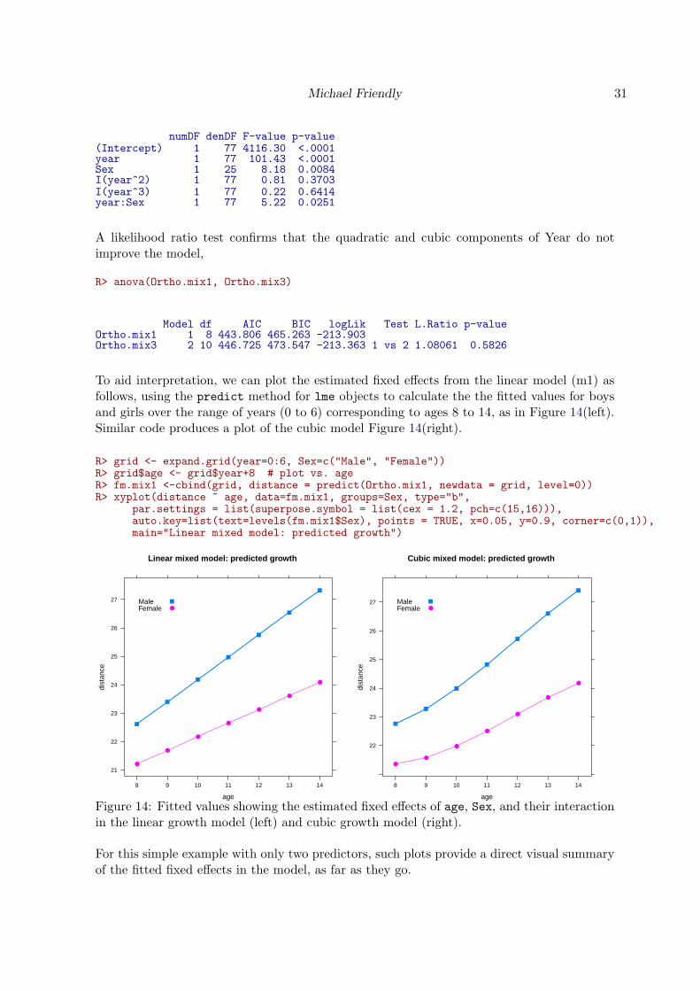
numDF denDF F-value p-value(Intercept) 1 77 4116.30 <.0001year 1 77 101.43 <.0001Sex 1 25 8.18 0.0084I(year^2) 1 77 0.81 0.3703I(year^3) 1 77 0.22 0.6414year:Sex 1 77 5.22 0.0251

A likelihood ratio test confirms that the quadratic and cubic components of Year do notimprove the model,

R> anova(Ortho.mix1, Ortho.mix3)

Model df AIC BIC logLik Test L.Ratio p-valueOrtho.mix1 1 8 443.806 465.263 -213.903Ortho.mix3 2 10 446.725 473.547 -213.363 1 vs 2 1.08061 0.5826

To aid interpretation, we can plot the estimated fixed effects from the linear model (m1) asfollows, using the predict method for lme objects to calculate the the fitted values for boysand girls over the range of years (0 to 6) corresponding to ages 8 to 14, as in Figure 14(left).Similar code produces a plot of the cubic model Figure 14(right).

R> grid <- expand.grid(year=0:6, Sex=c("Male", "Female"))R> grid$age <- grid$year+8 # plot vs. ageR> fm.mix1 <-cbind(grid, distance = predict(Ortho.mix1, newdata = grid, level=0))R> xyplot(distance ~ age, data=fm.mix1, groups=Sex, type="b",

par.settings = list(superpose.symbol = list(cex = 1.2, pch=c(15,16))),auto.key=list(text=levels(fm.mix1$Sex), points = TRUE, x=0.05, y=0.9, corner=c(0,1)),main="Linear mixed model: predicted growth")

Linear mixed model: predicted growth

age

dist

ance

21

22

23

24

25

26

27

8 9 10 11 12 13 14

●

●

●

●

●

●

●

MaleFemale ●

Cubic mixed model: predicted growth

age

dist

ance

22

23

24

25

26

27

8 9 10 11 12 13 14

●●

●

●

●

●

●

MaleFemale ●

Figure 14: Fitted values showing the estimated fixed effects of age, Sex, and their interactionin the linear growth model (left) and cubic growth model (right).

For this simple example with only two predictors, such plots provide a direct visual summaryof the fitted fixed effects in the model, as far as they go.

32 HE Plots for Repeated Measures Designs

7.2. MVLM approach

For the multivariate approach, the Orthodont data must first be reshaped to wide formatwith the distance values as separate columns.

R> library("nlme")R> Orthowide <- reshape(Orthodont, v.names="distance", idvar=c("Subject", "Sex"),

timevar="age", direction="wide")R> some(Orthowide, 4)

Subject Sex distance.8 distance.10 distance.12 distance.141 M01 Male 26 25.0 29.0 31.09 M03 Male 23 22.5 24.0 27.565 F01 Female 21 20.0 21.5 23.093 F08 Female 23 23.0 23.5 24.0

The MVLM is then fit as follows, with Sex as the between-S factor. Age is quantitative, sothe intra-subject data frame (idata) is created with age as an ordered factor.

R> Ortho.mod <- lm(cbind(distance.8, distance.10, distance.12, distance.14) ~ Sex, data=Orthowide)R> idata <- data.frame(age=ordered(seq(8,14,2)))R> Ortho.aov <- Anova(Ortho.mod, idata=idata, idesign=~age)R> Ortho.aov

Type II Repeated Measures MANOVA Tests: Pillai test statisticDf test stat approx F num Df den Df Pr(>F)

(Intercept) 1 0.9940 4123 1 25 < 2e-16 ***Sex 1 0.2710 9 1 25 0.00538 **age 1 0.8256 36 3 23 6.88e-09 ***Sex:age 1 0.2601 3 3 23 0.06960 .---Signif. codes: 0 ✬***✬ 0.001 ✬**✬ 0.01 ✬*✬ 0.05 ✬.✬ 0.1 ✬ ✬ 1

We see that both Sex and age are highly significant and their interaction is nearly significant.

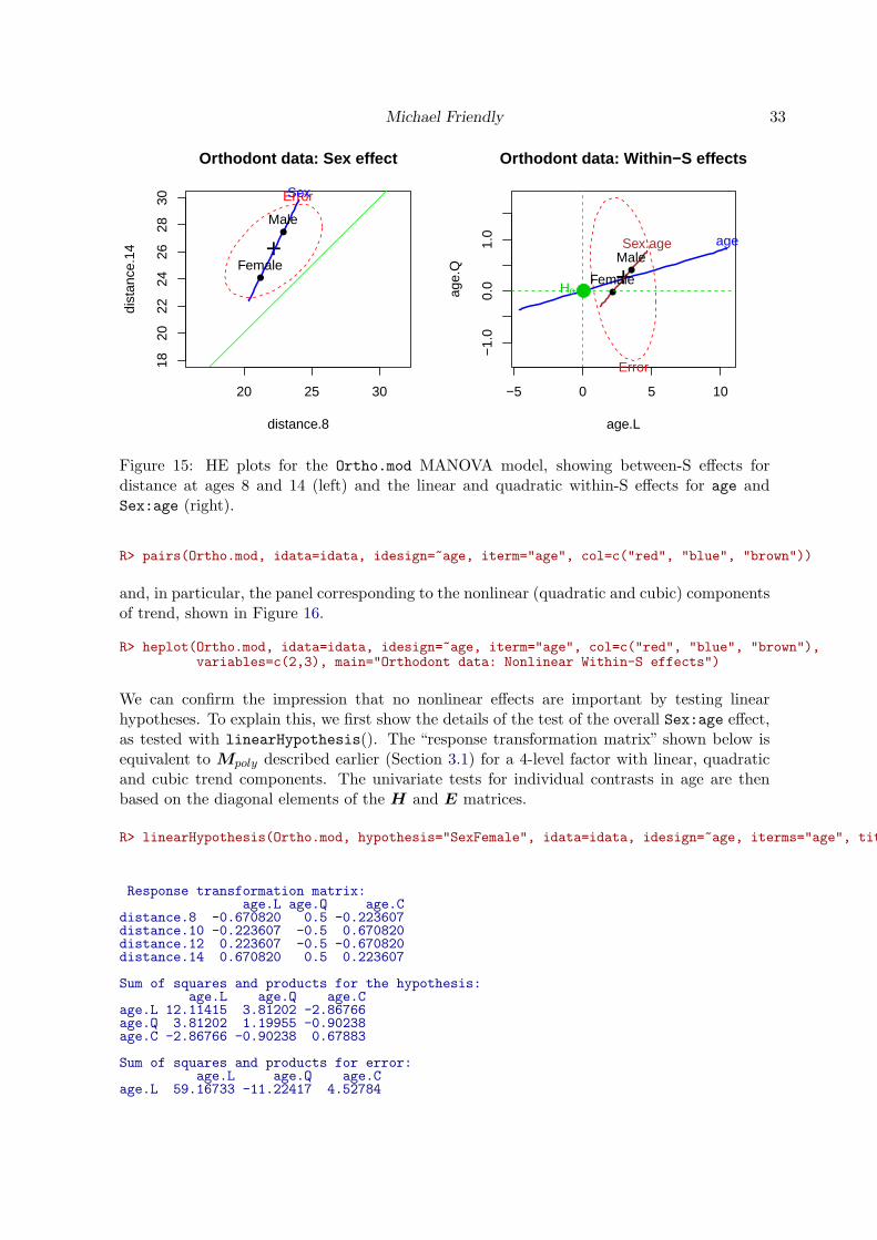
Figure 15 shows HE plots for the between- and within-S effects, produced as shown below.The left panel plots the effect of Sex for ages 8 and 14, with a green line of unit slope.Males clearly show greater growth by age 14, and the difference between males and femalesis greater at at 14 than at age 8. The right panel shows the linear and quadratic trends withage, reflecting the overall age main effect and the Sex:age interaction. Recalling that thecontributions of each displayed variable to each effect in an HE plot can be seen by theirhorizontal and vertical shadows relative to the E ellipse, we see that the main effect of ageis essentially linear, and the overall Sex:age effect is nearly significant due to a difference inslopes, but not curvature.

R> op <- par(mfrow=c(1,2))R> heplot(Ortho.mod, variables=c(1,4), asp=1, col=c("red", "blue"),

xlim=c(18,30), ylim=c(18,30),main="Orthodont data: Sex effect")

R> abline(0,1, col="green")R> heplot(Ortho.mod, idata=idata, idesign=~age, iterm="age", col=c("red", "blue", "brown"),

main="Orthodont data: Within-S effects")R> par(op)

To examine the questions of interest here in more detail, we focus on the intra-subject designand ask if linear growth is sufficient to explain both average development over time anddifferences between boys and girls. This is easily answered visually from the pairs() plot(not shown here),

Michael Friendly 33

20 25 30

1820

2224

2628

30Orthodont data: Sex effect

distance.8

dist

ance

.14 +

ErrorSex

●

●

Male

Female

−5 0 5 10

−1.

00.

01.

0

Orthodont data: Within−S effects

age.L

age.

Q +

Error

ageSex:age

●

●

Male

Female●H0

Figure 15: HE plots for the Ortho.mod MANOVA model, showing between-S effects fordistance at ages 8 and 14 (left) and the linear and quadratic within-S effects for age andSex:age (right).

R> pairs(Ortho.mod, idata=idata, idesign=~age, iterm="age", col=c("red", "blue", "brown"))

and, in particular, the panel corresponding to the nonlinear (quadratic and cubic) componentsof trend, shown in Figure 16.

R> heplot(Ortho.mod, idata=idata, idesign=~age, iterm="age", col=c("red", "blue", "brown"),variables=c(2,3), main="Orthodont data: Nonlinear Within-S effects")

We can confirm the impression that no nonlinear effects are important by testing linearhypotheses. To explain this, we first show the details of the test of the overall Sex:age effect,as tested with linearHypothesis(). The “response transformation matrix” shown below isequivalent to Mpoly described earlier (Section 3.1) for a 4-level factor with linear, quadraticand cubic trend components. The univariate tests for individual contrasts in age are thenbased on the diagonal elements of the H and E matrices.

R> linearHypothesis(Ortho.mod, hypothesis="SexFemale", idata=idata, idesign=~age, iterms="age", tit

Response transformation matrix:age.L age.Q age.C

distance.8 -0.670820 0.5 -0.223607distance.10 -0.223607 -0.5 0.670820distance.12 0.223607 -0.5 -0.670820distance.14 0.670820 0.5 0.223607

Sum of squares and products for the hypothesis:age.L age.Q age.C

age.L 12.11415 3.81202 -2.86766age.Q 3.81202 1.19955 -0.90238age.C -2.86766 -0.90238 0.67883

Sum of squares and products for error:age.L age.Q age.C

age.L 59.16733 -11.22417 4.52784

34 HE Plots for Repeated Measures Designs

−1.0 −0.5 0.0 0.5 1.0 1.5

−2

−1

01

2

Orthodont data: Nonlinear Within−S effects

age.Q

age.

C +

Error

ageSex:age

●

●

Male

Female

●H0

Figure 16: Nonlinear components of the within-S effects of age and Sex:age, showing thatthey are quite small in relation to within-S error.

age.Q -11.22417 26.04119 -1.28193age.C 4.52784 -1.28193 62.91932

Multivariate Tests: Sex:age effectDf test stat approx F num Df den Df Pr(>F)

Pillai 1 0.260113 2.69527 3 23 0.069604 .Wilks 1 0.739887 2.69527 3 23 0.069604 .Hotelling-Lawley 1 0.351557 2.69527 3 23 0.069604 .Roy 1 0.351557 2.69527 3 23 0.069604 .---Signif. codes: 0 ✬***✬ 0.001 ✬**✬ 0.01 ✬*✬ 0.05 ✬.✬ 0.1 ✬ ✬ 1

From this, the linear and nonlinear terms can be tested by selecting the appropriate columnsof Mpoly supplied as the contrasts associated with the age effect. For example, for tests ofthe linear effect of age and the Sex:age interaction (differences in slopes),

R> linear <- idataR> contrasts(linear$age, 1) <- contrasts(linear$age)[,1]R> print(linearHypothesis(Ortho.mod, hypothesis="(Intercept)",

idata=linear, idesign=~age, iterms="age", title="Linear age"), SSP=FALSE)

Multivariate Tests: Linear ageDf test stat approx F num Df den Df Pr(>F)

Pillai 1 0.76892 83.187 1 25 1.9862e-09 ***Wilks 1 0.23108 83.187 1 25 1.9862e-09 ***Hotelling-Lawley 1 3.32748 83.187 1 25 1.9862e-09 ***Roy 1 3.32748 83.187 1 25 1.9862e-09 ***---Signif. codes: 0 ✬***✬ 0.001 ✬**✬ 0.01 ✬*✬ 0.05 ✬.✬ 0.1 ✬ ✬ 1

R> print(linearHypothesis(Ortho.mod, hypothesis="SexFemale",idata=linear, idesign=~age, iterms="age", title="Linear Sex:age"), SSP=FALSE)

Michael Friendly 35

Multivariate Tests: Linear Sex:ageDf test stat approx F num Df den Df Pr(>F)

Pillai 1 0.169948 5.1186 1 25 0.032614 *Wilks 1 0.830052 5.1186 1 25 0.032614 *Hotelling-Lawley 1 0.204744 5.1186 1 25 0.032614 *Roy 1 0.204744 5.1186 1 25 0.032614 *---Signif. codes: 0 ✬***✬ 0.001 ✬**✬ 0.01 ✬*✬ 0.05 ✬.✬ 0.1 ✬ ✬ 1

Similarly, the nonlinear effects of age and the Sex:age interaction can be tested as follows,using the contrasts for quadratic and cubic trends in age.

R> nonlin <- idataR> contrasts(nonlin$age, 2) <- contrasts(nonlin$age)[,2:3]R> print(linearHypothesis(Ortho.mod, hypothesis="(Intercept)",

idata=nonlin, idesign=~age, iterms="age", title="Nonlinear age"), SSP=FALSE)

Multivariate Tests: Nonlinear ageDf test stat approx F num Df den Df Pr(>F)

Pillai 1 0.103180 1.38061 2 24 0.27069Wilks 1 0.896820 1.38061 2 24 0.27069Hotelling-Lawley 1 0.115051 1.38061 2 24 0.27069Roy 1 0.115051 1.38061 2 24 0.27069

R> print(linearHypothesis(Ortho.mod, hypothesis="SexFemale",idata=nonlin, idesign=~age, iterms="age", title="Nonlinear Sex:age"), SSP=FALSE)

Multivariate Tests: Nonlinear Sex:ageDf test stat approx F num Df den Df Pr(>F)

Pillai 1 0.052578 0.665952 2 24 0.52302Wilks 1 0.947422 0.665952 2 24 0.52302Hotelling-Lawley 1 0.055496 0.665952 2 24 0.52302Roy 1 0.055496 0.665952 2 24 0.52302

These examples show that, in simple cases, traditional plots of fitted values from mixed models(Figure 14) have the advantage of simple visual interpretation in terms of slopes and intercepts,at least for linear models. But such profile plots are generic: comparable plots could equallywell be drawn for the fitted values from the MVLM in this section. HE plots for repeatedmeasure designs have the additional advantage of showing the nature of significance tests andlinear hypotheses, though the structure of the MVLM requires separate plots of between-Sand within-S effects. In more complex designs with multiple between-S and within-S effects,and designs with multivariate responses (where mixed models do not apply), HE plots gaingreater advantage.

8. Discussion

Graphical methods for univariate response models are well-developed, but analogous methodsfor multivariate responses are still developing. Indeed, this is a fruitful area for new research(Friendly 2007). HE plots provide one new direction, providing direct visualizations of effectsin MVLMs, in the space of response variables (or in the the reduced-rank canonical space(candisc package) displaying maximal differences).

36 HE Plots for Repeated Measures Designs

This paper has shown how these methods can be extended to repeated measures designs, bydisplaying effects in the transformed space of contrasts or linear combinations for within-Seffects. As we hope to have shown, these plots can provide insights into the relations amongeffects and interpretations of those that are significant (or not) which go beyond what isavailable in traditional, univariate displays.

Acknowledgments

I am grateful to John Fox for collaboration, advice and continued development of the car

package which provides the computational infrastructure for the heplots package. The As-sociate Editor and one reviewer helped considerably in clarifying the presentation of thesemethods.

References

Dempster AP (1969). Elements of Continuous Multivariate Analysis. Addison-Wesley, Read-ing, MA.

Fox J (1987). “Effect Displays for Generalized Linear Models.” In CC Clogg (ed.), SociologicalMethodology, 1987, pp. 347–361. Jossey-Bass, San Francisco.

Fox J (2009). car: Companion to Applied Regression. R package version 1.2-16.

Fox J, Friendly M, Monette G (2007). heplots: Visualizing Tests in Multivariate Linear

Models. R package version 0.7-5.

Fox J, Friendly M, Monette G (2009). “Visualizing hypothesis tests in multivariate linearmodels: The heplots package for R.” Computational Statistics, 24(2), 233–246. (Publishedonline: 15 May 2008).

Fox J, Hong J (2009). “Effect Displays in R for Multinomial and Proportional-Odds LogitModels: Extensions to the effects Package.” Journal of Statistical Software, 32(1), 1–24.

Friendly M (2006). “Data Ellipses, HE Plots and Reduced-Rank Displays for MultivariateLinear Models: SAS Software and Examples.” Journal of Statistical Software, 17(6), 1–42.

Friendly M (2007). “HE plots for Multivariate General Linear Models.” Journal of Computa-

tional and Graphical Statistics, 16(2), 421–444.

Friendly M (2010). “HE Plots for Repeated Measures Designs.” Journal of Statistical Software,37(4), 1–37.

Friendly M, Fox J (2009). candisc: Generalized Canonical Discriminant Analysis. R packageversion 0.5-16.

Hsu PL (1938). “Notes on Hotelling’s generalized T.” The Annals of Mathematical Statistics,9, 231–243.

Michael Friendly 37

Monette G (1990). “Geometry of Multiple Regression and Interactive 3-D Graphics.” In J Fox,S Long (eds.), Modern Methods of Data Analysis, chapter 5, pp. 209–256. Sage Publications,Beverly Hills, CA.

O’Brien RG, Kaiser MK (1985). “MANOVA method for analyzing repeated measures designs:An extensive primer.” Psychological Bulletin, 97, 316–333.

Pinheiro JC, Bates DM (2000). Mixed-Effects Models in S and S-PLUS. Statistics andComputing Series. Springer-Verlag, New York, NY.

Potthoff RF, Roy SN (1964). “A Generalized Multivariate Analysis of Variance Model UsefulEspecially for Growth Curve Problems.” Biometrika, 51, 313–326.

R Development Core Team (2010). R: A Language and Environment for Statistical Comput-

ing. R Foundation for Statistical Computing, Vienna, Austria. ISBN 3-900051-07-0.

Rencher AC (1995). Methods of multivariate analysis. Wiley, New York, NY.

Timm NH (1975). Multivariate Analysis with Applications in Education and Psychology.Wadsworth (Brooks/Cole), Belmont, CA.

Timm NH (1980). “Multivariate Analysis of Variance of Repeated Measurements.” In PR Kr-ishnaiah (ed.), Handbook of Statistics, volume 1, chapter 2, pp. 41–87. North-Holland,Amsterdam.

Verbeke G, Molenberghs G (2000). Linear Mixed Models for Longitudinal Data. Springer,New York, NY.

Warnes GR (2009). gplots: Various R programming tools for plotting data. R package version2.7.4.

Affiliation:

Michael FriendlyPsychology DepartmentYork UniversityToronto, ON, M3J 1P3CanadaE-mail: friendly@yorku.caURL: http://datavis.ca