Repeated Measures ANOVA - University of Colorado …ibgcarey/p5741ndir/RM/RepeatedMeasures.pdf© 1998, Gregory Carey Repeated Measures ANOVA - 1 1 REPEATED MEASURES ANOVA Repeated

© 1998, Gregory Carey Repeated Measures ANOVA - 1

1

REPEATED MEASURES ANOVA

Repeated measures ANOVA (RM) is a specific type of MANOVA. When the withingroup covariance matrix has a special form, then the RM analysis usually gives more powerfulhypothesis tests than does MANOVA. Mathematically, the within group covariance matrix isassumed to be a type H matrix (SAS terminology) or to meet Huynh-Feldt conditions. Thesemathematical conditions are given in the appendix. Most software for RM prints out both theMANOVA results and the RM results along with a test of RM assumption about the withingroup covariance matrix. Consequently, if the assumption is violated, one can interpret theMANOVA results. In practice, the MANOVA and RM results are usually similar.

There are certain stock situations when RM is used. The first occurs when the dependentvariables all measure the same construct. Examples include a time series design of growth curvesof an organism or the analysis of number of errors in discrete time blocks in an experimentalcondition. A second use of RM occurs when all the dependent variables are all measured on thesame scale (e.g., the DVs are all Likert scale responses). For example, outcome from therapymight be measured on Likert scales reflecting different types of outcome (e.g., symptomamelioration, increase in social functioning, etc.). A third situation is for internal consistencyanalysis of a set of items or scales that purport to measure the same construct.. Internalconsistency analysis consists in fitting a linear model to a set of items that are hypothesized tomeasure the same construct. For example, suppose that you have written ten items that youthink measure the construct of empathy. Internal consistency analysis will provide measures ofthe extent to which these items "hang together" statistically and measure a single construct.(NOTE WELL: as in most stats, good internal consistency is just an index; you must be the judgeof whether the single construct is empathy or something else.) If you are engaged in this type ofscale construction, you should also use the SPSS subroutine RELIABILITY or SAS PROCCORR with the ALPHA option.

The MANOVA output from a repeated measures analysis is similar to output fromtraditional MANOVA procedures. The RM output is usually expressed as a "univariate"analysis, despite the fact that there is more than one dependent variable. The univariate RM hasa jargon all its own which we will now examine by looking at a specific example.

An example of an RM designConsider a simple example in which 60 students studying a novel foreign language are

randomly assigned to two conditions: a control condition in which the foreign language is taughtin the traditional manner and a experimental condition in which the language is taught in an


2

“immersed” manner where the instructor speaks only in the foreign language. Over the course ofa semester, five tests of language mastery are given. The structure of the data is given in Table 1.

Table 1. Structure of the data for a repeated measures analysis of language instruction.

Student Group Test 1 Test 2` Test 3 Test 4 Test 5Abernathy Control 17 22 26 28 31

. . . . . . .Zelda Control 18 24 25 30 29

Anasthasia Experimental 16 23 28 29 34. . . . . . .

Zepherinus Experimental 23 25 29 38 47

The purpose of such an experiment is to examine which of the two instructional techniques isbetter. One very simple way of doing this is to create a new variable that is the sum of the 5 testscores and perform a t-test. The SAS code would be

DATA rmex1; INFILE 'c:\sas\p7291dir\repeated.simple.dat'; LENGTH group $12.; INPUT subjnum group test1-test5; testtot = sum(of test1-test5);RUN;

PROC TTEST; CLASS group; VAR testtot;RUN;

The output from this procedure would be:

TTEST PROCEDUREVariable: TESTTOT

GROUP N Mean Std Dev Std Error--------------------------------------------------------------------------Control 30 154.43333333 27.96510551 5.10570637Experimental 30 170.50000000 32.91237059 6.00894926

Variances T DF Prob>|T|---------------------------------------Unequal -2.0376 56.5 0.0463Equal -2.0376 58.0 0.0462

For H0: Variances are equal, F' = 1.39 DF = (29,29) Prob>F' = 0.3855


3

The mean total test score for the experimental group (170.5) is greater than the mean total testscore for controls (154.4). The difference is significant (t = -2.04, df = 58, p < .05) so we shouldconclude that the experimental language instruction is overall superior to the traditional languageinstruction.

There is nothing the matter with this analysis. It gives an answer to the major questionposed by the research design and suggests that in the future, the experimental method should beadopted for foreign language instruction.

But the expense of time in generating the design of the experiment and collecting the datamerit much more than this simple analysis. One very interesting question to ask is whether themeans for the two groups change over time. Perhaps the experimental instruction is good initiallybut poor at later stages of foreign language acquisition. Or maybe the two techniques start outequally but diverge as the semester goes on. A simple way to answer these questions is toperform separate t-tests for each of the five tests. The code here would be:

PROC TTEST DATA=rmex1; CLASS GROUP; VAR test1-test5;RUN;

A summary of these results is given in Table 2.

Table 2. Group means and t-test results for the 5tests.

Means:Test Control Experimental t p <

1 20.17 18.80 .70 .492 27.8 29.1 -.59 .563 30.7 36.1 -2.66 .014 36.83 40.43 -1.90 .075 38.93 46.07 -3.35 .002

At this stage a plot of the means is helpful.

Both the plot of the means and the t-test results suggest that the two groups start out


4

fairly similar at times 1 and times 2, diverge significantly at time 3, are almost significantlydifferent at time 4, and diverge again at time 5. This analysis gives more insight, but leads to itsown set of problems. We have performed 5 different significance tests. If these tests wereindependent—and they are clearly nor independent because they were performed on the same setof individuals—then we should adjust the α level by the Bonferroni formula

α adjustednumber of tests= − = − =1 95 1 95 01

12. . .. .

Using this criterion, we would conclude that the differences in test 3 are barely significant, thosein test 4 are not significant, while the means for the last test are indeed different. Perhaps themajor reason why the two groups differ is only on the last exam in the course.

A repeated measures example can help to clarify the situation. The advantage to RM isthat it will control for the correlations among the tests and come up with an overall test for eachof the hypotheses given above. The RM design divides ANOVA factors into two types:between subjects factors (or effects) and within subject factors (or effects). If you think of the rawdata matrix, you should have little trouble distinguishing the two. A single between subjectsfactor has one and only one value per observation. Thus, group is a between subjects factorbecause each observation in the data matrix has only one value for this variable (Control orExperimental).

Within subjects factors have more than one value per observation. Thus, time of test is awithin subject factor because each subject has five difference values--Test1 through Test5.Another way to look at the distinction is that between subject factors are all the independentvariables. Within subject factors involve the dependent variables. All interaction terms thatinvolve a within subject factor are included in within subject effects. Thus, interactions of time oftest with group is a within subject effect. Only interactions that include only between subjectfactors are included in between subjects effects.

The effects in a RM ANOVA are the same as those in any other ANOVA. In the presentexample, there would be a main effect for group, a main effect for time and an interaction betweengroup and time. RM differs only in the mathematics used to compute these effects.

At the expense of putting the cart before the horse, the SAS commands to perform therepeated measures for this example are:

TITLE Repeated Measures Example 1;PROC GLM DATA=rmex1; CLASS group; MODEL test1-test5 = group; MEANS group; REPEATED time 5 polynomial / PRINTM PRINTE SUMMARY;RUN;


5

As in an ANOVA or MANOVA, the CLASS statement specifies the classificationvariable which is group in this case. The MODEL statement lists the dependent variables (onthe left hand side of the equals sign) and the independent variables (on the right hand side). TheMEANS statement asks that the sample size, means, and standard deviations be output for thetwo groups.

The novel statement in this example is the REPEATED statement. Later, this statementwill be discussed in detail. The current REPEATED statement gives a name for the repeatedmeasures or within subjects factor—time in this case—and the number of levels of that factor—5in this example because the test was given over 5 time periods. The word polynomial instructsSAS to perform a polynomial transform of the 5 dependent variables. Essentially this creates 4“new” variables from the original 5 dependent variables. (Any transformation of k dependentvariables will result in k - 1 new transformed variables.) The PRINTM option prints thetransformation matrix, the PRINTE option prints the error correlation matrix and some otherimportant output, and the SUMMARY option prints ANOVA results for each of the fourtransformed variables.

Usually it is the transformation of the dependent variables that gives the RM analysisadditional insight into the data. Transformations will be discussed at length later. Here we justnote that the polynomial transformation literally creates 4 new variables from the 5 originaldependent variables. The first of the new variables is the linear effect of time; it tests whetherthe means of the language mastery tests increase or decrease over time. The second new variableis the quadratic effect of time. This new variable tests whether the means have a single “bend” tothem over time. The third new variable is the cubic effect over time; this tests for two “bends” inthe plot of means over time. Finally the fourth new variable is the quartic effect over time, and ittests for three bends in the means over time.

The first few pages of output from this procedure give the results from the univariateANOVAs for test1 through test5. Because there are only two groups, the F statistics for theseanalysis are equal to the square of the t statistics in Table 2 and the p values for the ANOVAswill be the same as those in Table 2. Hence these results are not presented. The rest of theoutput begins with the MEANS statement.


6

---<PAGE>-------------------------------------------------------------------Repeated Measures Example 1 7General Linear Models Procedure

Level of -----------TEST1---------- -----------TEST2----------GROUP N Mean SD Mean SDControl 30 20.1666667 7.65679024 27.8000000 7.76996871Experimental 30 18.8000000 7.46208809 29.1000000 9.12499410

Level of -----------TEST3---------- -----------TEST4----------GROUP N Mean SD Mean SDControl 30 30.7000000 6.88902175 36.8333333 7.06659618Experimental 30 36.1000000 8.70334854 40.4333333 7.57347155

Level of ------------TEST5------------GROUP N Mean SDControl 30 38.9333333 8.65401375Experimental 30 46.0666667 7.80332968

---<PAGE>-------------------------------------------------------------------Repeated Measures Example 1 8General Linear Models ProcedureRepeated Measures Analysis of VarianceRepeated Measures Level Information

Dependent Variable TEST1 TEST2 TEST3 TEST4 TEST5 Level of TIME 1 2 3 4 5

The following section of output shows the design of the repeated measure factor. It is quitesimple in this case. You should always check this to make certain that design specified on theREPEATED statement is correct.


7

---<PAGE>-------------------------------------------------------------------Repeated Measures Example 1 9General Linear Models ProcedureRepeated Measures Analysis of Variance

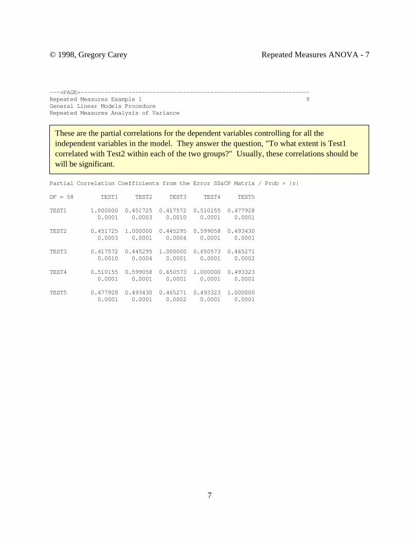
Partial Correlation Coefficients from the Error SS&CP Matrix / Prob > |r|

DF = 58 TEST1 TEST2 TEST3 TEST4 TEST5

TEST1 1.000000 0.451725 0.417572 0.510155 0.477928 0.0001 0.0003 0.0010 0.0001 0.0001

TEST2 0.451725 1.000000 0.445295 0.599058 0.493430 0.0003 0.0001 0.0004 0.0001 0.0001

TEST3 0.417572 0.445295 1.000000 0.650573 0.465271 0.0010 0.0004 0.0001 0.0001 0.0002

TEST4 0.510155 0.599058 0.650573 1.000000 0.493323 0.0001 0.0001 0.0001 0.0001 0.0001

TEST5 0.477928 0.493430 0.465271 0.493323 1.000000 0.0001 0.0001 0.0002 0.0001 0.0001

These are the partial correlations for the dependent variables controlling for all theindependent variables in the model. They answer the question, "To what extent is Test1correlated with Test2 within each of the two groups?" Usually, these correlations should bewill be significant.


8

TIME.N represents the nth degree polynomial contrast for TIME

M Matrix Describing Transformed Variables TEST1 TEST2 TEST3 TEST4 TEST5TIME.1 -.6324555320 -.3162277660 0.0000000000 0.3162277660 0.6324555320TIME.2 0.5345224838 -.2672612419 -.5345224838 -.2672612419 0.5345224838TIME.3 -.3162277660 0.6324555320 -.0000000000 -.6324555320 0.3162277660TIME.4 0.1195228609 -.4780914437 0.7171371656 -.4780914437 0.1195228609

E = Error SS&CP MatrixTIME.N represents the nth degree polynomial contrast for TIME TIME.1 TIME.2 TIME.3 TIME.4TIME.1 1723.483333 -2.521377 236.550000 313.306091TIME.2 -2.521377 2187.726190 98.502728 35.622692TIME.3 236.550000 98.502728 1657.950000 -468.112779TIME.4 313.306091 35.622692 -468.112779 1715.000476

Below is the transformation matrix. It is printed here because the PRINTM option wasspecified in the REPEATED statement. Because we specified a POLYNOMIALtransformation, this matrix gives coefficients for what are called orthogonal polynomials. They are analogous but not identical to contrast codes for independent variables. The firstnew variable, TIME.1, gives the linear effect over time, the second, TIME.2 is the quadraticeffect, etc.


9


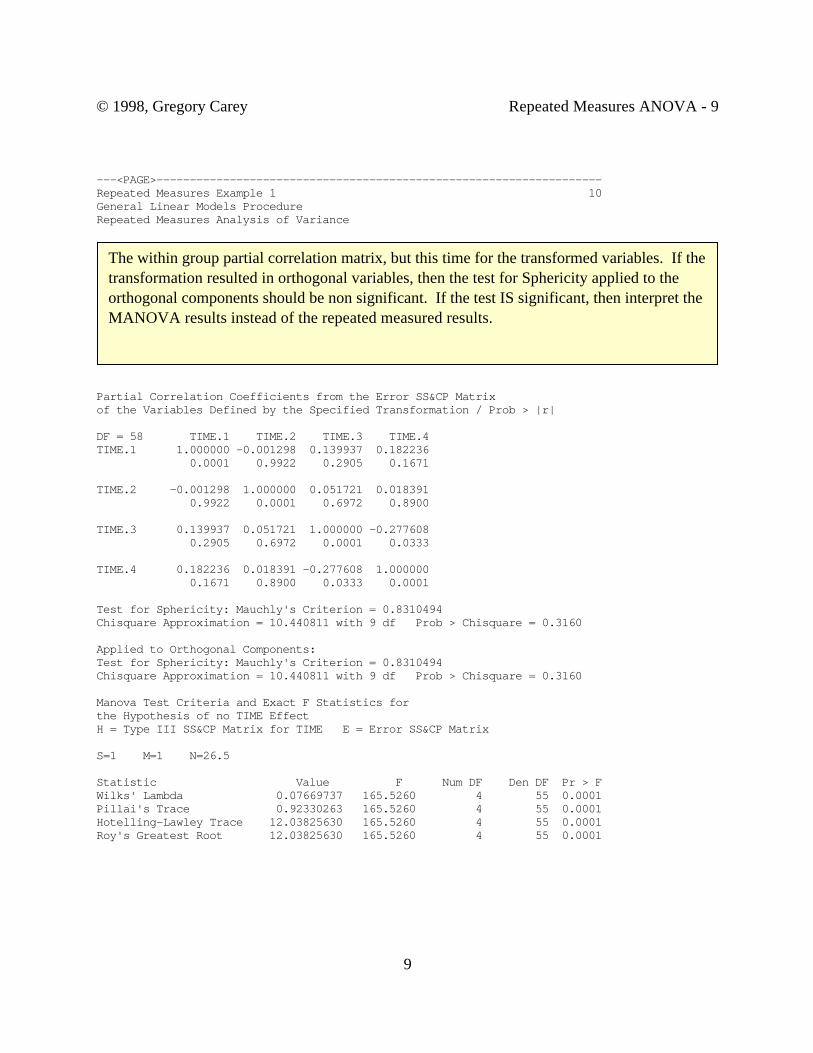
Partial Correlation Coefficients from the Error SS&CP Matrixof the Variables Defined by the Specified Transformation / Prob > |r|

DF = 58 TIME.1 TIME.2 TIME.3 TIME.4TIME.1 1.000000 -0.001298 0.139937 0.182236 0.0001 0.9922 0.2905 0.1671

TIME.2 -0.001298 1.000000 0.051721 0.018391 0.9922 0.0001 0.6972 0.8900

TIME.3 0.139937 0.051721 1.000000 -0.277608 0.2905 0.6972 0.0001 0.0333

TIME.4 0.182236 0.018391 -0.277608 1.000000 0.1671 0.8900 0.0333 0.0001

Test for Sphericity: Mauchly's Criterion = 0.8310494Chisquare Approximation = 10.440811 with 9 df Prob > Chisquare = 0.3160

Applied to Orthogonal Components:Test for Sphericity: Mauchly's Criterion = 0.8310494Chisquare Approximation = 10.440811 with 9 df Prob > Chisquare = 0.3160

Manova Test Criteria and Exact F Statistics forthe Hypothesis of no TIME EffectH = Type III SS&CP Matrix for TIME E = Error SS&CP Matrix

S=1 M=1 N=26.5

Statistic Value F Num DF Den DF Pr > FWilks' Lambda 0.07669737 165.5260 4 55 0.0001Pillai's Trace 0.92330263 165.5260 4 55 0.0001Hotelling-Lawley Trace 12.03825630 165.5260 4 55 0.0001Roy's Greatest Root 12.03825630 165.5260 4 55 0.0001

The within group partial correlation matrix, but this time for the transformed variables. If thetransformation resulted in orthogonal variables, then the test for Sphericity applied to theorthogonal components should be non significant. If the test IS significant, then interpret theMANOVA results instead of the repeated measured results.


10


Manova Test Criteria and Exact F Statistics forthe Hypothesis of no TIME*GROUP EffectH = Type III SS&CP Matrix for TIME*GROUP E = Error SS&CP Matrix

S=1 M=1 N=26.5

Statistic Value F Num DF Den DF Pr > FWilks' Lambda 0.74044314 4.8200 4 55 0.0021Pillai's Trace 0.25955686 4.8200 4 55 0.0021Hotelling-Lawley Trace 0.35054260 4.8200 4 55 0.0021Roy's Greatest Root 0.35054260 4.8200 4 55 0.0021Repeated Measures Example 1 12

General Linear Models ProcedureRepeated Measures Analysis of VarianceTests of Hypotheses for Between Subjects Effects

Source DF Type III SS Mean Square F Value Pr > FGROUP 1 774.4133 774.4133 4.15 0.0462Error 58 10818.5733 186.5271


11

---<PAGE>-------------------------------------------------------------------Repeated Measures Example 1 13General Linear Models ProcedureRepeated Measures Analysis of VarianceUnivariate Tests of Hypotheses for Within Subject Effects

Source: TIME Adj Pr > F DF Type III SS Mean Square F Value Pr > F G - G H - F 4 19455.82000000 4863.95500000 154.92 0.0001 0.0001 0.0001

Source: TIME*GROUP Adj Pr > F DF Type III SS Mean Square F Value Pr > F G - G H - F 4 674.02000000 168.50500000 5.37 0.0004 0.0005 0.0004

Source: Error(TIME) DF Type III SS Mean Square 232 7284.16000000 31.39724138

Greenhouse-Geisser Epsilon = 0.9332 Huynh-Feldt Epsilon = 1.0225

---<PAGE>-------------------------------------------------------------------Repeated Measures Example 1 14General Linear Models ProcedureRepeated Measures Analysis of VarianceAnalysis of Variance of Contrast Variables

TIME.N represents the nth degree polynomial contrast for TIME

Contrast Variable: TIME.1

Source DF Type III SS Mean Square F Value Pr > FMEAN 1 18961.88167 18961.88167 638.12 0.0001GROUP 1 558.73500 558.73500 18.80 0.0001Error 58 1723.48333 29.71523

Contrast Variable: TIME.2Source DF Type III SS Mean Square F Value Pr > FMEAN 1 421.4583333 421.4583333 11.17 0.0015GROUP 1 18.6011905 18.6011905 0.49 0.4853Error 58 2187.7261905 37.7194171




12

The RM design divides ANOVA factors into two types: between subjects factors (oreffects) and within subject factors (or effects). If you think of the above type of data matrix, youshould have little trouble distinguishing the two. Between subjects factors have one and only onevalue per observation. Thus, Mode, Type, and Age are between subjects factors. Within subjectsfactors have more than one value per observation. Thus, Test is a within subject factor becauseeach subject has five difference values--Test1 through Test5. Another way to look at thedistinction is that between subject factors are all the independent variables. Within subject factorsare the dependent variables. All interaction terms that involve a within subject factor are includedin within subject effects. Thus, interactions of test with mode, test with type, and test with agewould be considered a within subject effect. Only interactions that include only between subjectfactors are included in between subjects effects. Thus, the interaction of mode with type or modewith age are between subject effects.

The between subjects effects answers the following question: why does one subject'saverage score over the five tests differ from another subject's average score? In the above design,there are several possible reasons--the effect of Mode, the effect of Type, the effect of Age, andany interactions among these three. The within subjects effects ask why the five tests mightdiffer for any single subject. There are several reasons. First, the tests might differ in difficulty--aTest effect. One Mode of instruction might make it easier to master some parts of the languageearlier than others--a Test by Mode interaction. Some Types might affect early versus latemastery--a Test by Type interaction. And learning curves might depend upon age--an Age byTest interaction. One could even construct higher order interactions, say a Test by Mode byType by Age interaction. All of these interactions are included in the within subjects effectsbecause they all include an interaction with Test, a within subjects factor.

In order to test for univariate within subjects effects using RM, it is necessary totransform the dependent variables. We have already seen one type of transformation ofdependent variables in profile analysis in MANOVA. There are several other types oftransformations useful for RM. They are discussed below in the section on transformations.

Transformations: Why Do Them?

The primary reason for transforming the dependent variables in RM is to generatevariables that are more informative than the original variables. Consider the RM example. Thedependent variables are tests of language mastery. Scores on a mastery test should be low early in


13

the course and increase over the course. At some point, we might expect them to asymptote,depending upon the difficulty of the mastery test. We can then reformulate the researchquestions into the following set of questions: Do some types of instruction increase mastery at afaster rate than other types? Does computer based instruction increase mastery at a faster ratethan classroom instruction? To answer these questions, we want to compare the independentvariables on the linear increase over time in mastery test scores. If the mastery test is constructedso that scores asymptote at some time point during the course, we could ask the followingquestions: Do some types of instructions asymptote faster than other types? Or, does computerbased instruction asymptote faster than classroom instruction? To answer these questions, wewant to test the differences in the quadratic effect over time for the independent variables. Inshort, we want to transform the test scores so that the first transformed variable is the lineareffect over time and the second variable is the quadratic effect over time. We can then do aMANOVA or RM on the transformed variables.

There are also statistical reasons for transformations1. We can see the statisticalphilosophy behind transformations by recalling the major reason for using MANOVA instead ofinterpreting a series of univariate analyses. We use MANOVA because dependent variables arecorrelated. If we get obsessional about the whole business and want to interpret a series ofunivariate analyses, then the best way of doing that is to transform the dependent variables insuch a way that they are uncorrelated. This is one good statistical reason for transforming thevariables in RM.

We also want the variances of the transformed variables to be homogeneous. The reasonfor this is that we would like to have one single overall F for the dependent variables to determinewhether or not there are significant effects. We cannot get an exact F statistic unless the variancesof the dependent variables are homogeneous. The situation is analogous to a simple univariate F 1 The real justification for the transformation is to test whether the covariance matrix has aparticular form that will make the F statistic exact. An identity matrix has this form and a matrixwith homogeneous variances (all diagonal elements equal) and homogeneous covariances (all offdiagonal elements equal) also has this form. But there are other matrices that will also permitrepeated measures. One characteristic common to all these matrices is that an orthonormaltransformation of the dependent variables gives an expected correlation matrix that is an identitymatrix. The interested reader is referred to Huynh, H. and Feldt, L.S. (1970), Conditions underwhich mean square ratios in repeated measurements designs have exact F-distributions. Journal ofthe American Statistical Association, 65, 1582-1589.


14

test for, say, three groups. In order for the F test to be valid the variances of the four groupsmust be homogeneous. In RM, the variances of the dependent variables must be homogeneous.One way to achieve homogeneity of variances is to transform the dependent variables so thattheir variances are unity.

Thus, two ideal statistical requirements of transformation are that: (1) the variances areunity, and (2) the transformed variables are uncorrelated. If we can achieve this, we have anorthonormalized transformation. Some types of transformations will guarantee that thedependent variables will be orthonormalized--e.g., rescaled principal components. However, thetransformations most often used in RM designs do not always guarantee that the transformeddependent variables will in fact be orthonormalized. Hence, we must always test whether thetransformation has worked. In order to do this, we compare the transformed covariance matrix toan identity matrix using a test called a sphericity test. There are several types of sphericity tests,but all are estimates of a likelihood ratio c2. [The tests differ in how they adjust the c2 for the factthat in small samples, the likelihood ratio c2 is not asymptotically valid.] Both SAS and SPSSxwill spit out sphericity tests upon request. If the test is significant, then the transformation hasnot worked. If the test is not significant, then most researchers assume the transformation hasworked and will interpret the results of the univariate RM. Most sphericity tests are regarded asa "sensitive" test. That is, they will often give "statistical significance" even though there is littlesubstantive difference between the correlation matrix for the transformed variables and anidentity matrix.

If the transformation gives a significant c2, there are several options to choose from:

(1) ignore it because the matrix is pretty close to an identity matrix. (Notrecommended because picky journal editors and referees often get upset over this,even though there might not be anything wrong with it.)

(2) use the MANOVA results to interpret the within subjects effects.

(3) use the Greenhouse - Geisser correction or the Huynh - Feldt correction to theunivariate F statistics. Both of these are adjustments to the degrees of freedom foran F statistic to take into account the fact that the covariance matrix does not meetthe strict requirements of RM. SAS prints these two corrections and theirassociated F statistics under the respective labels 'G - G' and 'H - F'. SAS alsoprints out the Greenhouse - Geisser ε and the Huyhn - Feldt ε. Both of these


15

statistics index the extent to which the transformed matrix meets the requirementsof the RM design. In the ideal case where the requirements are exactly met to thenth decimal place, then ε should equal 1.0. The value of ε gets small andapproaches 0 as the requirements are more and more violated.


16

Transformations: How to Do Them

Both SAS and SPSSx recognize that constructing transformation matrices is a real pain inthe gluteus to the max. Thus, they do it for you. As a user of a RM design, your major obligationis to choose the transformation that makes the most sense for your data. SAS will automaticallyperform the following transformations for you:

CONTRAST. A CONTRAST transformation compares each level of the repeated measureswith the first level. It is useful when the first level represents a control or baseline level ofresponse and you want to compare the subsequent levels to the baseline. For our example, thefirst transformed variable will be the (Test1 - Test2), the second transformed variable will be(Test1 - Test3), the third (Test1 - Test4) and the last (Test1 - Test5). CONTRAST is thedefault transformation in SAS--the one you get if you do not specify a transformation.

MEAN. A MEAN transformation compares a level with the mean of all the other levels. It ismostly useful if you haven't the vaguest idea of how to transform the repeated measuresvariables. For the example, the first transformed variable will be (Test1 - mean of [Test2 + Test3+ Test4 + Test5]), the second variable will be (Test2 - mean of [Test1 + Test3 + Test4 +Test5]), etc. Note that there is always one less transformation than the number of variables.Hence, if you use a MEAN transform in SAS, you will not get the last level contrasted with themean of the other levels. If you have a burning passion to do this, see the PROC GLMdocumentation in the SAS manual.

PROFILE. A PROFILE transformation compares a level against the next level. It is sometimesuseful in testing responses that are not expected to increase or decrease regularly over time. Forthe example, the first transformed variable is (Test1 - Test2), the second is (Test2 - Test3), thethird is (Test3 - Test4), etc.

HELMERT. A HELMERT transform compares a level to the mean of all subsequent levels. Thisis a very useful transformation when one wants to pinpoint when a response changes over time.For our example, the first transformed variable would be (Test1 - mean of [Test2 + Test3 +Test4 + Test5]), the second would be (Test2 - mean of [Test3 + Test4 + Test5]), the thirdwould be (Test3 - mean of [Test4 + Test5]), and the last would simply be (Test4 - Test5). If theunivariate F statistics were significant for the first and second transformed variables but notsignificant for the third and fourth, then we would conclude that language mastery was achieved


17

by the time of the third test.

POLYNOMIAL. A POLYNOMIAL transform fits orthogonal polynomials. Like a Helmerttransform, this is useful to pinpoint changes in response over time. It is also useful when therepeated measures are ordered values of a quantity, say the dose of a drug. The first transformedvariable represents the linear effect over time (or dose). The second transformed variable denotesthe quadratic effect, the third the cubic effect, etc. If you are familiar enough with polynomials tointerpret the observed means in light of linear, quadratic, cubic, etc. effects, this is anexceptionally useful transformation. Often, one can predict beforehand the order of thepolynomial but not the exact time period where the response might be maximized (or minimized).

SPSSx will also transform repeated measures variables using the CONTRAST subcommand tothe MANOVA procedure. Note, however, that terminology and procedures differ greatlybetween SAS and SPSSx. Be particularly careful of the CONTRAST statement. In SAS, theCONTRAST statement refers to a transformation of only the independent variables. TheCONTRAST option on the REPEATED statement allows for a specific type of transformationfor repeated measures variables. SPSSx views a CONTRAST as a transformation of eitherindependent variables or dependent variables, depending upon the context. To make the issuemore confusing, SPSSx has another subcommand, TRANSFORM, that applies only to thedependent variables. Also, both packages will do a "profile" transformation, but actually dodifferent transformations. You should always consult the appropriate manual before evertransforming the repeated measures variables.


18

Interpreting Repeated Measures

To interpret repeated measures results, it is helpful to create a table of the effects.Suppose that the model we fit for our example was based on the following SAS statements:

PROC GLM DATA=INSTRUC;CLASS MODE TYPE;MODEL TEST1--TEST5 = MODE TYPE MODE*TYPE AGE;

Then we can construct a Table that looks like this:

p values from:

ANOVA Effects MANOVA F F GG F HF F

Between Subjects:MODETYPEMODE*TYPEAGE

Within Subjects:TIMEMODE*TIMETYPE*TIMEMODE*TYPE*TIMEAGE*TIMEERROR

Here the variable TIME is used to denote the set of the five tests.2 We now want to fill inthe p values from the various F statistics. The between subjects effects are equivalent to theeffects from an ANOVA using an individual's average score (or total score) on the five tests asthe dependent variable. Consequently, all the F statistics and their associated p values will be the 2 Belatedly, I note that I switched terms here. The TIME effect in this analysis is the same asthe TEST effect referred to in the previous sections.


19

same for the between subjects effects. For the within subjects effects, however, the F statisticsand associated p values will generally differ.

The within subjects effects are interpreted as if they were ANOVA factors. The TIMEeffect within subjects tells us whether the means for the five tests are equal. The MODE*TIMEwithin subject effect has the same interpretation as a MANOVA using MODE as theindependent variable and the five tests (TIME) as the dependent variables. That is, are the (5 by1) vector of means on the five tests for the Classroom condition and the (5 by 1) vector of meanson the five tests for the Computer condition sampled from the same distribution? TheTYPE*TIME within subject factor tests whether the three (5 by 1) vectors of means for theEmpirical, Programmed, and Didactic condition are pulled from the same hat. TheMODE*TYPE*TIME effect tests whether the six (5 by 1) vectors of means for the two Modesand three Types are different from those predicted on the basis of knowing a Mode effect and aTime effect. Finally, the AGE*TIME effect tests whether the five regression coefficients forAGE are the same for all five tests.

We can now fill in the table from the computer output. Here, I have chosen to put in the pvalue associated with Wilk's l for the multivariate F.


20

p values from:

ANOVA Effects MANOVA F F GG F HF F

Between Subjects:MODE .31TYPE .10MODE*TYPE .80AGE .0001

Within Subjects:TIME .03 .02 .02 .02MODE*TIME .56 .67 .66 .67TYPE*TIME .0001 .0001 .0001 .0001MODE*TYPE*TIME .66 .63 .62 .63AGE*TIME .99 .99 .99 .99ERROR

To interpret the table, we first need to examine the test of sphericity. For this problem, c2

= 12.0 (df = 9, p = .21). This suggests that the correlation matrix among the variables has theappropriate form that permits the more powerful F test to be used. Were the c2 significant, thenwe would ignore the column for the F and interpret the columns for the MANOVA, theGreenhouse-Geiser correction, and the Huyhn-Feldt correction.

As it stands, all four test statistics yield the same result. If the four columns differed, thenchoose the column for F when the sphericity test is passed. If the test is not passed, then youmust make a decision based on the other three columns, and there is no established criteria forchoosing among the three. The G-G correction is the most conservative, especially in smallsamples. That is, you are less likely to reject a null hypothesis with this test than with theMANOVA or the H-F correction.

Now let's interpret the substance of these results. For the total score over the five tests(the between subjects factors), there is no effect for Mode, Type, or their interaction. This meansthat average mastery levels over the course of the semester does not depend upon the way inwhich students were instructed. Age, however, is significant, so average mastery is predicted bystudent's age.


21

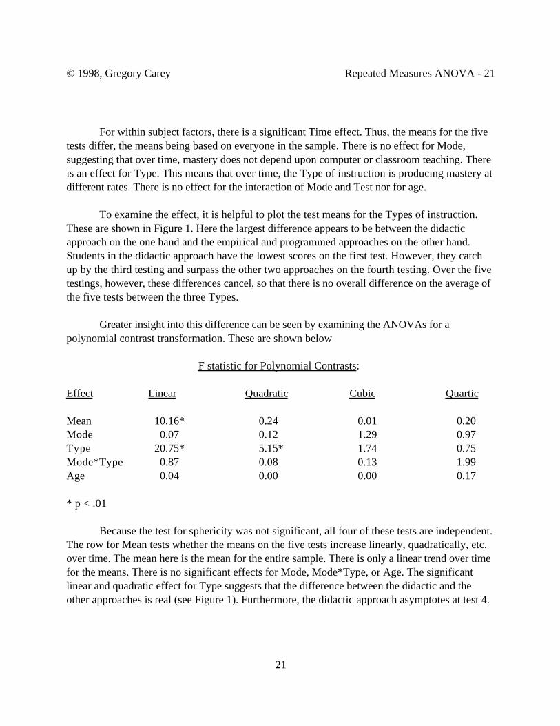
For within subject factors, there is a significant Time effect. Thus, the means for the fivetests differ, the means being based on everyone in the sample. There is no effect for Mode,suggesting that over time, mastery does not depend upon computer or classroom teaching. Thereis an effect for Type. This means that over time, the Type of instruction is producing mastery atdifferent rates. There is no effect for the interaction of Mode and Test nor for age.

To examine the effect, it is helpful to plot the test means for the Types of instruction.These are shown in Figure 1. Here the largest difference appears to be between the didacticapproach on the one hand and the empirical and programmed approaches on the other hand.Students in the didactic approach have the lowest scores on the first test. However, they catchup by the third testing and surpass the other two approaches on the fourth testing. Over the fivetestings, however, these differences cancel, so that there is no overall difference on the average ofthe five tests between the three Types.

Greater insight into this difference can be seen by examining the ANOVAs for apolynomial contrast transformation. These are shown below

F statistic for Polynomial Contrasts:

Effect Linear Quadratic Cubic Quartic

Mean 10.16* 0.24 0.01 0.20Mode 0.07 0.12 1.29 0.97Type 20.75* 5.15* 1.74 0.75Mode*Type 0.87 0.08 0.13 1.99Age 0.04 0.00 0.00 0.17

* p < .01

Because the test for sphericity was not significant, all four of these tests are independent.The row for Mean tests whether the means on the five tests increase linearly, quadratically, etc.over time. The mean here is the mean for the entire sample. There is only a linear trend over timefor the means. There is no significant effects for Mode, Mode*Type, or Age. The significantlinear and quadratic effect for Type suggests that the difference between the didactic and theother approaches is real (see Figure 1). Furthermore, the didactic approach asymptotes at test 4.


22

Therefore, the deflection in the straight line from Time 4 to Time 5 is real compared to the lack ofdeflection in either the empirical or programmed approaches.

Thus, at the end of a semester, students appear to achieve the same levels of foreignlanguage mastery regardless of the Mode or Type of teaching. However, the approach to thismastery depends upon the Type of instruction. Empirical and programmed learning strategiestend to linearly increase mastery over time. A didactic approach, on the other hand, achievesmastery sooner than the other two, but is more difficult at the early stages of learning.

Repeated Measures / Within Subjects Designs: A quick & dirty approach

Background: There are probably as many different ways to perform repeated measures analysisas there are roads that lead to Rome. Furthermore, there are just as many differences interminology. Here the term "repeated measures" is used synonymously with "within subjects."Thus, within subjects factors are the same as repeated measures factors. Also note that the SASuse of a "contrast" transformation for repeated measures is not the same as contrast coding astaught by Chick and Gary. Here, the term "transformation" is used to refer to the creation of newdependent variables from the old dependent variables. [Sorry about all this but I did not make upthe rules.] The following is one quick and dirty way to perform a repeated measures ANOVA (orregression). There are several other ways to accomplish the same task, so there is no "right" or"wrong" way as long as the correct model is entered and the correct statistics interpreted.


23

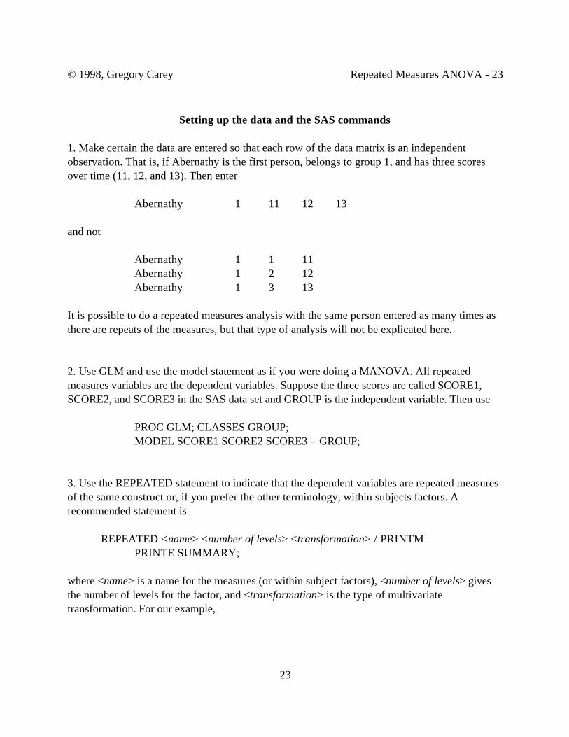
Setting up the data and the SAS commands

1. Make certain the data are entered so that each row of the data matrix is an independentobservation. That is, if Abernathy is the first person, belongs to group 1, and has three scoresover time (11, 12, and 13). Then enter

Abernathy 1 11 12 13

and not

Abernathy 1 1 11Abernathy 1 2 12Abernathy 1 3 13

It is possible to do a repeated measures analysis with the same person entered as many times asthere are repeats of the measures, but that type of analysis will not be explicated here.

2. Use GLM and use the model statement as if you were doing a MANOVA. All repeatedmeasures variables are the dependent variables. Suppose the three scores are called SCORE1,SCORE2, and SCORE3 in the SAS data set and GROUP is the independent variable. Then use

PROC GLM; CLASSES GROUP;MODEL SCORE1 SCORE2 SCORE3 = GROUP;

3. Use the REPEATED statement to indicate that the dependent variables are repeated measuresof the same construct or, if you prefer the other terminology, within subjects factors. Arecommended statement is

REPEATED <name> <number of levels> <transformation> / PRINTMPRINTE SUMMARY;

where <name> is a name for the measures (or within subject factors), <number of levels> givesthe number of levels for the factor, and <transformation> is the type of multivariatetransformation. For our example,


24

REPEATED TIME 3 POLYNOMIAL / PRINTM PRINTE SUMMARY;

will work just fine.

When there is more than a single repeated measures factor, then you must specify them inthe correct order. For example, suppose the design called for a comparison of recall versusrecognition memory for phrases that are syntactically easy, moderate, and hard to remember.Each subject has 2 x 3 = 6 scores. Suppose Abernathy's scores are arranged in the following way:

Recall RecognitionEasy Mod Hard Easy Mod Hard

Group Y1 Y2 Y3 Y4 Y5 Y6

Abernathy 1 12 8 3 21 16 14

The SAS statements should be:

PROC GLM; CLASSES GROUP; MODEL Y1-Y6 = GROUP; REPEATED MEMTYPE 2, DIFFCLTY 3 POLYNOMIAL / PRINTM PRINTE

SUMMARY;

There we specify two repeated measures factors (or within subjects factors). The first isMEMTYPE for recall versus recognition memory, and the second is DIFFCLTY and to denotethe difficulty level of the phrases, . Note that the factor that changes least rapidly alwayscomes first. Had we specified DIFFCLTY 3, MEMTYPE 2, then SAS would have interpretedY1 as Recall-Easy, Y2 as Recognition-Easy, Y3 as Recall-Moderate, etc.

4. Remember that using a REPEATED statement will always generate a transformation of thevariables. Always choose the type of transformation that will reveal the most meaningfulinformation about your data.


25

5. That is all there is to doing a repeated measures ANOVA or Regression. You can use theCONTRAST statement if you wish to contrast code categorical independent variables. Just makecertain that you place the CONTRAST statement before the REPEATED statement.

Interpreting the Output

This is a synopsis of the handout on Repeated Measures. You should follow these stepsto interpret the output.

1. The first thing SAS writes in the output is the design for the repeated measures. Always checkthis to make certain that correctly specified the levels of the repeated measures. This isparticularly important when there is more than a single within subjects factor.

2. The second thing to check is whether error covariance matrix can be orthogonally transformed.The tests of sphericity will tell you that. Some transformations in SAS are deliberately set up tobe orthogonal (e.g., POLYNOMIAL with no further qualifiers); other transformations are notorthogonal (e.g., CONTRAST). If a transformation is orthogonal, then SAS will print out onetest of sphericity. If a transformation is not orthogonal, then SAS spits out two tests ofsphericity. The first test is for the straight transformation. The second test is for the orthogonalcomponents of the transformation. In this case, it is the second test--the one for the orthogonalcomponents--that you want to interpret.

3. If the c2 test for sphericity is not significant, then ignore all the MANOVA output andinterpret the RM ANOVA results for the within subjects effects. These are labelled in the SASoutput as "Univariate Tests of Hypotheses for Within Subjects Effects."

4. If the c2 test for sphericity was significant, then you can interpret the MANOVA results orthe adjusted probability levels from Greenhouse-Geisser and the Huynh-Feldt corrections for thewithin subjects effects. If is often a good idea to compare the MANOVA significance with theGreenhouse-Geisser and the Huynh-Feldt adjusted significance levels to make certain there isagreement between them.

5. The between subjects effects are not affected by the results of the sphericity test. Hence, SASoutput with the heading "Tests of Hypotheses for Between Subjects Effects" will always becorrect.


26

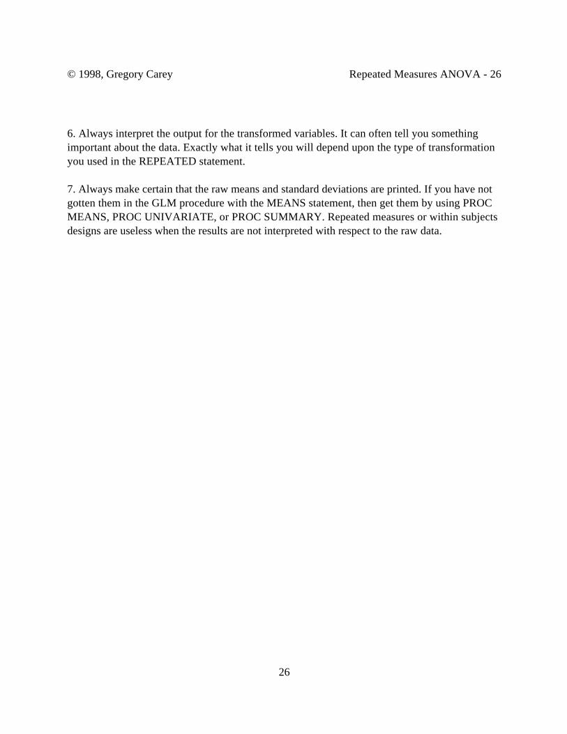
6. Always interpret the output for the transformed variables. It can often tell you somethingimportant about the data. Exactly what it tells you will depend upon the type of transformationyou used in the REPEATED statement.

7. Always make certain that the raw means and standard deviations are printed. If you have notgotten them in the GLM procedure with the MEANS statement, then get them by using PROCMEANS, PROC UNIVARIATE, or PROC SUMMARY. Repeated measures or within subjectsdesigns are useless when the results are not interpreted with respect to the raw data.

Documents

Repeated Measures ANOVA - University of Colorado …ibgcarey/p5741ndir/RM/RepeatedMeasures.pdf© 1998, Gregory Carey Repeated Measures ANOVA - 1 1 REPEATED MEASURES ANOVA Repeated