Multivariate Analysis,Clustering, and Classification

Jessi CisewskiYale University

Astrostatistics Summer School 2017

1

Multivariate Analysis

Statistical analysis of data containing observations each with > 1variable measured.

Examples:

1 Measurements on a star: luminosity, color, environment,metallicity, number of exoplanets

2 Functions such as light curves and spectra

3 Images

2

Common goals

1 Describe the p-dimensional distribution

Multivariate means, variances, and covariances

Multivariate probability distributions

2 Reduce the number of variables without losing significantinformation

Linear functions of variables (principal components)

3 Investigate dependence between variables

4 Statistical inference

Confidence regions, multivariate regression, hypothesis testing

5 Clustering and Classification

3

Organizing the data

p = number of variables

n = number of observations

xij = i th observation of the j th variable

Variables

Observations

1 2 · · · p1 x11 x12 · · · x1p2 x21 x22 · · · x2p...

......

. . ....

n xn1 xn2 · · · xnp

4

Data matrix:

X =

x11 x12 · · · x1px21 x22 · · · x2p

......

. . ....

xn1 xn2 · · · xnp

This can also be written as n rows or as p columns

X =

xT1xT2...

xTn

=[

x1, x2, · · · , xp]

5

Descriptive statistics

Sample mean of the j th variable

x·j =1

n

n∑i=1

xij

Sample mean vector

x =

x1x2...xp

6

Sample covariance of variables i and j

sij = sji =1

n − 1

n∑k=1

(xki − x·i )(xkj − x·j)

Sample variance of the j th variable is sjj

Sample covariance matrix

S =

s11 s12 · · · s1ps21 s22 · · · s2p...

.... . .

...sp1 sp2 · · · spp

7

Sample correlation coefficient of variables i and j

rij =sij√sii sjj

rii = 1 and rij = rji

Sample correlation matrix

R =

1 r12 · · · r1pr21 1 · · · r2p...

.... . .

...rp1 rp2 · · · 1

8

Caution

Correlations measure the strength of the linear relationshipsbetween variables if such relationships are valid.

9

Multivariate Probability Distributions

Goal: make probability statements about random vectors

p-dimensional random vector:

X =

X1

X2...Xp

where X1, . . . ,Xp are random variables.

X is a continuous random vector if X1, . . . ,Xp are all continuousrandom variables

We’ll focus on continuous random vectors

10

Three important properties of X’s probability density function, f

1 f (x) ≥ 0 for all x ∈ Rp (or wherever the x’s take values)

2 The total area below the function f is 1:∫Rp

f (x)dx = 1

3 For all t1, t2, . . . , tp,

P(X1 ≤ t1,X2 ≤ t2, . . . ,Xp ≤ tp) =

∫ t1

−∞

∫ t2

−∞· · ·∫ tp

−∞f (x)dx

11

Recall: an expected value is an average over the entire population

Mean vector:

µ =

µ1µ2...µp

where

µi = E (Xi ) =

∫Rp

xi f (x)d(x)

is the mean of the ith component of X

12

Covariance between Xi and Xj :

σij = E (Xi − µi )(Xj − µj) = E (XiXj)− µiµj

And the variance of each Xi is:

σii = E (Xi − µi )2 = E (X 2i )− µ2i

Covariance matrix of X:

Σ =

σ11 σ12 · · · σ1pσ21 σ22 · · · σ2p

......

. . ....

σp1 σp2 · · · σpp

Σ = E (X− µ)(X− µ)T = E (XX)T = µµT

Going forward, let’s assume Σ is nonsingular

13

Multivariate Normal Distribution

Consider the following random vector whose possible values rangeover all of ∈Rp:

X =

X1

X2...Xp

X has a multivariate normal distribution if it has a pdf of the form

f (X) =1

(2π)p2 |Σ|

12

exp

[−1

2(X− µ)TΣ−1(X− µ)

]X ∼ Np(µ,Σ)

14

Image: http://en.wikipedia.org

15

Special case: diagonal Σ

Σ =

σ21 0 · · · 00 σ22 · · · 0...

.... . .

...0 0 · · · σ2p

In this case, X1, . . . ,Xp are mutually independent and normallydistributed with density

f (x) =

p∏j=1

{1

(2πσ2j )1/2e− 1

2σ2j

(xj−µj )2}

16

χ2 Distribution

X ∼ Np(µ,Σ) with pdf

f (X) =1

(2π)p2 |Σ|

12

exp

[−1

2(X− µ)TΣ−1(X− µ)

]

Then (X− µ)TΣ−1(X− µ) ∼ χ2p

17

Tests for multivariate normality

If the data contain a substantial number of outliers then it goesagainst the hypothesis of multivariate normality

If one variable is not normally distributed, then the full set ofvariables does not have a multivariate normal distribution

A possible resolution is to transform the original variables toproduce new variables which are normally distributed

Example: Box-Cox transformations

When datasets arise from a multivariate normal distribution, wecan perform accurate inference on its mean vector and covariancematrix

18

Variables (random vector): X ∼ Np(µ,Σ)

The parameters µ and Σ are unknown

Data (measurements): x1, x2, . . . , xn

Goal: estimate µ and Σ

x is an unbiased estimator of µ (and the MLE of µ)

The MLE of Σ is n−1n S → this is not unbiased (i.e. it is biased)

The sample covariance matrix, S , is an unbiased estimator of Σ

19

Principal Components Analysis (PCA)

Data: X = p-dimensional random vector with covariance matrix Σ

PCA is an unsupervised approach to learning about X

Principal components find directions of variability in X

Can be used for visualization, dimension reduction, regression, etc.

Image: http://cogsci.ucd.ie

20

Statistical LearningLearning from data

1 Unsupervised learning

2 Supervised learning

3 ...

21

?One? schematic for addressing problems in machine learning...

Image: Andy’s Computer Vision and Machine Learning Blog http://peekaboo-vision.blogspot.com

22

Clustering

Find subtypes or groups that are not defined a priori based onmeasurements

−→ “Unsupervised learning” or “Learning without labels”

Classification

Use a priori group labels in analysis to assign new observations to aparticular group or class

−→ “Supervised learning” or “Learning with labels”

∗ Some content and notation used throughout derived from notes by Rebecca

Nugent (CMU), Ryan Tibshirani (CMU), and textbooks Hastie et al. (2009)

and James et al. (2013).

23

Clustering and Classification

24

Sample Data

“data1”ng <- 50

set.seed(321) #ensures same dataset

g1 <- cbind(rnorm(ng,-3,.1), rnorm(ng,1,1))

g2 <- cbind(rnorm(ng,3,.1), rnorm(ng,1,1))

gtemp <- cbind(rnorm(ng*2,0,.75), rnorm(ng*2,0,.75))

rad1 <- sqrt(gtemp[,1]^2+gtemp[,2]^2)

g3 <- gtemp[order(rad1)[1:ng],]

g4 <- gtemp[order(rad1)[(ng+1):(2*ng)],]

g5.1<-seq(-2.75,2.75, length.out = ng)

g5.2 <- (g5.1/2)^2 - 4

g5 <- cbind(g5.1,g5.2 + rnorm(ng,0,.5))

data1<-rbind(g1,g2,g3,g4,g5)

labels1<-c(rep(1,ng),rep(2,ng),rep(3,ng),rep(4,ng),rep(5,ng))

This dataset will be used to illustrate clustering and classificationmethodologies throughout the lecture.

25

Good references

An Introduction to Statistical Learning (James et al. 2013)

−→ good introduction to get started using methods/not technical

The Elements of Statistical Learning (Hastie et al. 2009)

−→ very thorough and technical coverage of statistical learning

All of Statistics (Wasserman 2004)

−→ great overview of statistics

26

CLUSTERINGGrouping of similar objects (unsupervised learning)−→ members of the same cluster are “close” in some sense

Pattern recognition

Data segmentation

27

Clustering in Astronomy

→ Use properties of GRBs (e.g. lo-cation in the sky, arrival time, du-ration, fluence, spectral hardness) tofind subtypes/classes of events

Image: Mukherjee et al. (1998)

Image: http://science.hq.nasa.gov

→ Regions with an excess ofgamma rays that correspond to lo-cations of dwarf galaxies could beevidence of particle dark matter

28

Clustering set-up

Notation: given vectors X = {X1,X2, . . . ,Xn} ∈ Rp

−→ n observations in p - dimensional space−→ Variables/features/attributes indexed by j = 1, . . . , p: jthvariable is Xj

−→ Observations indexed by i = 1, . . . , n: ith variable is Xi

Want to learn properties about thejoint distribution P(X) of these vectors:organize, summarize, categorize, explain

No direct measure of success (e.g. no no-tion of a misclassification rate) −→ Suc-cessful if true structure is captured...

Image:

http://20102250.blogspot.com

29

General goals of clustering

Partition observations such that

1 Observations within a cluster are similar

“Compactness Property”

2 Observations in different clusters are non similar

“Closeness Property”

? Typically want compact clusters that are well-separated ?

30

Dissimilarity Measure

Characterizes degree of “closeness”

Dissimilarity matrix D = {dii ′} such that dii = 0 and

d jii ′ = d(xij , xi ′j)

Some examples of d jii ′ are (xij − xi ′j)

2 or |xij − xi ′j |

Dii ′ = D(Xi ,Xi ′) =∑p

j=1 wj · d jii ′ where

∑pj=1 wj = 1

31

Dissimilarity Measure: within cluster variation

Total cluster variability =1

2

n∑i=1

n∑i ′=1

Dii ′

=1

2

K∑k=1

∑C(i)=k

∑C(i ′)=k

Dii ′ +∑

C(i ′) 6=k

Dii ′

where C (i) = k is the assignment of observation i to cluster k

Total within cluster variability: 12

∑Kk=1

∑C(i)=k

∑C(i ′)=k Dii ′

Total between cluster variability: 12

∑Kk=1

∑C(i)=k

∑C(i ′)6=k Dii ′

32

Clustering methods

1 Combinatorial algorithms1 K - means clustering2 Hierarchical clustering

2 Mixture modeling/Statistical clustering (parametric)

3 Mode seeking/Bump Hunting/Statistical clustering(nonparametric)

33

K-means Clustering

Image: http://www.holehouse.org/mlclass/13_Clustering.html

34

K-means clustering

Main idea: partition observations in K separate clusters thatdo not overlap

35

K-means clustering - procedure

Goal: minimize total within-cluster scatter usingDii ′ =

∑pj=1(xij − xi ′j)

2 = ||Xi − Xi ′ ||2.

Then the within-cluster scatter is written as

1

2

K∑k=1

∑C(i)=k

∑C(i ′)=k

||Xi − Xi ′ ||2 =K∑

k=1

|Ck |∑

C(i)=k

||Xi − Xk ||2

|Ck | = number of observations in cluster Ck

Xk = (X k1 , . . . , X

kp )

36

K-means clustering - recipe

Pick K (number of clusters)

Select K centers

Alternate between the following:1 Assign each observation to closest center2 Recalculate centers

R: kmeans(data, K, nstart = 20)

37

Simple code: K-means

set.seed(321)

g1 <- cbind(rnorm(50,0,1), rnorm(50,-1,.1))

g2 <- cbind(rnorm(50,0,1), rnorm(50,1,.1))

g3 <- cbind(rnorm(50,0,1), rnorm(50,3,.1))

data.points <- rbind(g1, g2, g3)

km.out <- kmeans(data.points,3, nstart = 20)

plot(data.points, pch = 16, xlab = "X1", ylab = "X2", col = km.out$cluster)

points(km.out$centers[,1], km.out$centers[,2],pch=4,lwd=4, col="blue", cex = 2)

−→ Try moving the clusters closer together (in terms of X2) and seewhat happens with the K-means clusters.

38

K-means clustering - determining K

Choose the k that has the last “significant” reduction in the withingroups sum of squares (i.e. find the “elbow”)

set.seed(123); wss <- c(); number.k <- c(1:15)

for(ii in number.k){km0 <- kmeans(data1,ii,nstart = 20)

wss[ii] <- km0$tot.withinss}

plot(number.k, wss, xlab="K",ylab="WSS", type = "b", pch = 19)

39

K-means clustering - tips

Can be unstable; solution depends on starting set of centers−→ finds local optima, but want global optima−→ start with different centers kmeans(x, K, nstart = 20)

Cluster assignments are strict −→ no notion of degree or strengthof cluster membership

Possible lack of interpretability of centers−→ centers are averages:

- OK for clustering things like apartment prices based on price,square footage, distance to nearest grocery store

- But what if observations are images of faces?

Images: http://cdn1.thefamouspeople.com,http://www.notablebiographies.com,http:

//mrnussbaum.com,http://3.bp.blogspot.com 40

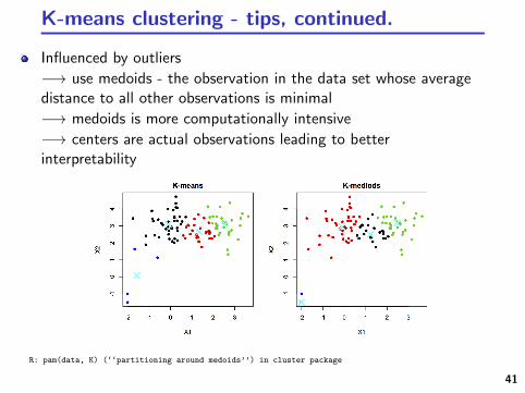
K-means clustering - tips, continued.

Influenced by outliers

−→ use medoids - the observation in the data set whose averagedistance to all other observations is minimal

−→ medoids is more computationally intensive

−→ centers are actual observations leading to betterinterpretability

R: pam(data, K) (‘‘partitioning around medoids’’) in cluster package

41

Hierarchical Clustering

Image: http://en.wikipedia.org/wiki/Hierarchical_clustering

42

Hierarchical vs. Flat Partitions

1 Flat partitioning (e.g. K-means clustering)

partitions data into K clusters; K determined by userno sense of the relationships among the clusters

2 Hierarchical partitioning

Generates a hierarchy of partitions; user selects the partitionP1 = 1 cluster, . . ., Pn = n clusters (agglomerative clustering)Partition Pi is the union of one or more clusters from PartitionPi+1

43

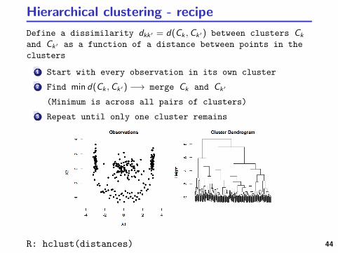
Hierarchical clustering - recipe

Define a dissimilarity dkk′ = d(Ck ,Ck′) between clusters Ck

and Ck′ as a function of a distance between points in the

clusters

1 Start with every observation in its own cluster

2 Find min d(Ck ,Ck′) −→ merge Ck and Ck′

(Minimum is across all pairs of clusters)

3 Repeat until only one cluster remains

R: hclust(distances) 44

Hierarchical clustering - distances

1 Friends-of-friends = Single-linkage clustering: intergroupdistance is smallest possible distance

d(Ck ,Ck ′) = minx∈Ck ,y∈Ck′

d(x , y)

2 Complete-linkage clustering: intergroup distance is largestpossible distance

d(Ck ,Ck ′) = maxx∈Ck ,y∈Ck′

d(x , y)

3 Average-linkage clustering: average intergroup distance

d(Ck ,Ck ′) = Avex∈Ck ,y∈Ck′d(x , y)

4 Ward’s clustering

d(Ck ,Ck ′) =2 (|Ck | · |Ck ′ |)|Ck |+ |Ck ′ |

||XCk− XCk′ ||

2

45

Single-linkage clustering

46

data1

47

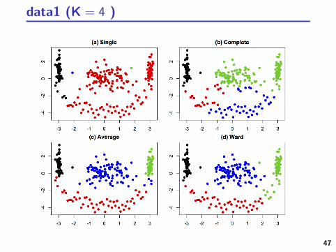
data1 (K = 4 )

47

Clustering Recap

1 Algorithmic clustering (no statistical assumptions)1 K-means2 Hierarchical linkage

2 Statistical clustering1 Parametric - associates a specific model with the density (e.g.

Gaussian, Poisson)−→ parameters associated with each cluster

2 Nonparametric - looks at contours of the density to find clusterinformation (e.g. kernel density estimate)

48

Mixture Modeling/Parametric Statistical Clustering

Image: Li and Henning (2011)

49

Model-based clustering (parametric)

Assumes that each subgroup/cluster/component in the populationhas its own density

p(X ) =K∑

k=1

πkpk(X ; θk)

where∑K

k=1 πk = 1 and 0 ≤ πk ≤ 1.

−→ Entire dataset is modeled by a mixture of these distributions.

p(x) = 0.5φ(x ; 4; 1) + 0.5φ(x ; 0; 1) (middle plot)p(x) = 0.75φ(x ; 4; 1) + 0.25φ(x ; 0; 1) (right plot)

50

Model-based clustering: Gaussian example

Suppose there are K clusters - each cluster is modeled by a particular

distribution (e.g. a Gaussian distribution with parameters µk , Σk)

The density of each cluster k is

pk(X ) = φ(X | µk ,Σk)

=1√

(2π)p|Σk |exp

(−

(X − µk)TΣ−1k (X − µk)

2

)

Letting πk be the weight of cluster k , the mixture density is

p(X ) =K∑

k=1

πkpk(X ) =K∑

k=1

πkφ(X | µk ,Σk)

51

Model-based clustering: advantages

1 Well-studied statistical inference techniques available

2 Flexibility in choosing the component distributions

3 Obtain a density estimate for each cluster

4 Soft classification is available

52

Model-based clustering: fitting the model

Suppose there are K clusters - each cluster is modeled by a particular

distribution (e.g. a Gaussian distribution with parameters µk , Σk)

Expectation - Maximization (EM) algorithm

Finds maximum likelihood estimates in incomplete data (e.g.missing cluster labels).

Alternates between expectation step and maximization steps:

E-step: compute conditional expectation of the cluster labels

M-step: maximize the likelihood and estimate parametersgiven the current labels; update parameter estimates

53

Model-based clustering: EM algorithm

Observations {X1,X2, . . . ,Xn} are incomplete (i.e. no labels)

Complete observations: {(X1,Y1), (X2,Y2), . . . , (Xn,Yn)}(where Yi are the labels)

The collections of parameters, θ are (πk , µk ,Σk) fork = 1, . . . ,K

The log-likelihood function is

l(X1, . . . ,Xn | θ) =n∑

i=1

log

(K∑

k=1

πkφ(xi | µk ,Σk)

)

l(X1, . . . ,Xn | θ) is the objective function of the EMalgorithm. Numerical difficulty comes from the sum inside thelog.

Goal: get MLEs for (πk , µk ,Σk), k = 1, . . . ,K

54

Nonparametric Clustering

Image: Feigelson et al. (2011) 55

Nonparametric clustering

Associate groups with high frequency areas −→ groups in thepopulation correspond to modes of the density p(x)

Goal: find the modes of the density p(x), or p(x). Assignobservations to the “domain of attraction” of a mode.

56

Nonparametric clustering

Associate groups with high frequency areas −→ groups in thepopulation correspond to modes of the density p(x)

Goal: find the modes of the density p(x), or p(x). Assignobservations to the “domain of attraction” of a mode.

56

Nonparametric clustering

Associate groups with high frequency areas −→ groups in thepopulation correspond to modes of the density p(x)Goal: find the modes of the density p(x), or p(x). Assignobservations to the “domain of attraction” of a mode.

?NP clustering is very dependent on the density estimate p(x)56

Final comment on selecting K

Slide from Ryan Tibshirani’s lecture, which was from George Cassella’s CMU seminar on 1/16/2011. 57

Final comment on selecting K

Slide from Ryan Tibshirani’s lecture, which was from George Cassella’s CMU seminar on 1/16/2011.57

Concluding Remarks: clustering

Clustering - unsupervised/no labels → find structure1 K - means2 Agglomerative hierarchical clustering3 Parametric/Nonparametric

58

CLASSIFICATIONBuild a model, classifier, etc. to separate data into knowngroups/classes (supervised learning)

Response variable is not continuous −→ want to predict labels

1 Bayes classifiers

2 K Nearest Neighbors (KNN) classifiers

3 Logistic regression

4 Linear Discriminant Analysis (LDA)

5 Support Vector Machines (SVM)

6 Tree classifiers

59

Classification in Astronomy

Stars can be classified into OBFGKMLTY

Image: https://writescience.files.wordpress.com

Classification of Active galactic nuclei (e.g. Starburst, Seyfert (I or II),Quasars, Blazars, BL Lac, OVV, Radio)

Galaxies can be classified into Hubble mor-phological types (E/S0/S/Irr), clustering en-vironments, and by star formation activity

Image: http://en.wikipedia.org

60

Classification set-up

Notation: given vectors X = {X1,X2, . . . ,Xn} ∈ Rp and classlabels Y = {y1, y2, . . . , yn}−→ the yi ’s are qualitative−→ let yi be the predicted class label for observation i−→ main interest is P(Y | X)

The classification training error rate is often estimated using atraining dataset as

1

n

n∑i=1

I(yi 6= yi )

where I(·) is the indicator function.

The classification test error rate is often estimated using a testdataset, (xtest , ytest) as

E (I(ytest 6= ytest))

−→ good classifiers have small test errors

61

Bayes Classifiers

Test error is minimized by assigning observations with predictors xto the class that has the largest probability:

P(Y = j | X = x)

for classes j = 1, . . . , J

If there are two classes (J = 2), the Bayes decision rule givenpredictors x is

yi =

{class 1 if P(Y = 1 | X = x) > 0.50class 2 if P(Y = 2 | X = x) > 0.50

?In general, intractable because the distribution of Y | X isunknown.

62

Image: http://vlm1.uta.edu/~athitsos/nearest_neighbors/

63

K Nearest Neighbors (KNN)

Main idea: An observation is classified based on the Kobservations in the training set that are nearest to it

A probability of each class can be estimated by

P(Y = j | X = x) = K−1∑

i∈N(x)

I(yi = j)

where j = 1, . . ., #classes in training set, and I = indicatorfunction.

K = 3 nearest neighbors to the Xare within the circle.

The predicted class of X would beblue because there are more blueobservations than green amongthe 3 NN.

64

KNN: data1

R: knn(training.set, test.set, training.set.labels, K) in class

package 65

KNN: data1 decision boundary

Using all observations of data1, K = 1

66

Linear Classifiers−→ Decision boundary is linear

Logistic regression

Linear Discriminant Analysis

Image: http://fouryears.eu/2009/02/

67

Logistic Regression

Predicting two groups: binary labels

Y =

{1 with probability π0 with probability 1− π

E [Y ] = P(Y = 1) = π

We assume the following model for logistic regression

logit(π) = log

(π

1− π

)= β0 + βTX

where β0 ∈ R, β ∈ Rp

68

Logistic Regression, continued.

logit(π) = log

(π

1− π

)= β0 + βTX

=⇒ π =eβ0+β

TX

1 + eβ0+βTX

Can fit β0, . . . , βp via MLE

l(β0, β) =∑n

i=1 log (P(Y = yi | X = xi )) =⇒

(β0, β) = argmaxβ0∈R,β∈Rp

n∑i=1

[yi · (β0 + βT xi )− log(1 + eβ0+β

T xi )]

69

Logistic Regression for data1

logit.labels = matrix(0, nrow = length(labels1))

logit.labels[c(which(labels1 == 2), which(labels1 == 5))] <- 1

logit.fit <- glm(logit.labels ~ data1[,1]+data1[,2],family = binomial)

summary(logit.fit) #<---provides details of the fit model

logit.fit.probs <- predict(logit.fit, type = "response")

logit.class = matrix(0,nrow = length(logit.fit.probs))

logit.class[logit.fit.probs >=.5] = 1

par(mfrow = c(1,2))

plot(data1, xlim = c(-4,4), ylim = c(-5,4), xlab = "X1", ylab = "X2", col = logit.labels+1,

pch = logit.labels+1, lwd = 3, main = "True classes")

plot(data1, xlim = c(-4,4), ylim = c(-5,4), xlab = "X1", ylab = "X2", col = logit.class+1,

pch = logit.class+1, lwd = 3, main = "Predicted classes")

70

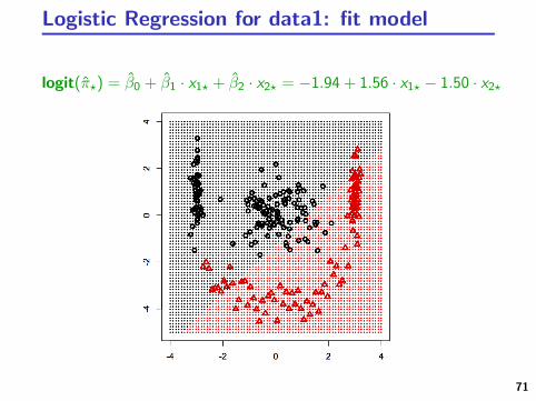
Logistic Regression for data1: fit model

logit(π?) = β0 + β1 · x1? + β2 · x2? = −1.94 + 1.56 · x1? − 1.50 · x2?

71

Multiple classes

What do we do if our response is not binary (i.e. J > 2)?

There are extensions of logistic regression for multiple classes:Multiple - class logistic regression

Linear Discriminant Analysis (LDA) is another option

72

Discriminant Analysis

Goal: estimate a decision boundary that gives a classification rule

Basic idea: estimate the posterior probabilities of class membership

−→ If an observation is in a particular location, what is theprobability it belongs to a particular class

Bayes’ Rule

P(Y = j ′ | x) =πj ′ · pj ′(x)∑Jj=1 πj · pj(x)

πj = prior probabilities of class j

pj(x) = P(X = x | Y = j)

−→ Need a way to estimate pj(x) in order to do classification

73

Example using Bayes’ Rule

Consider X = 1.9, P(Y = 1) =

12 · 0.065

12 · 0.065 + 1

2 · 0.219≈ 0.229

23 · 0.065

23 · 0.065 + 1

3 · 0.172≈ 0.274

74

Linear Discriminant Analysis (LDA)

Multivariate Gaussian

pj(X ) = φ(X | µj ,Σj)

=1√

(2π)p|Σj |exp

(−

(X − µj)TΣ−1j (X − µj)2

)

LDA assumes all covariance matrices are equal (Σ1 = · · · = ΣJ)

75

LDA continued

A predictor x is classified in the class j = 1, . . . , J according to thefollowing:

argmaxj{P(Y = j | X = x)} =

= argmaxj{φ(x | µj ,Σ)πj}

= argmaxj{log (φ(x | µj ,Σ)πj)}

...

= argmaxj

{−1

2(x − µj)TΣ−1(x − µj) + log(πj)

}= argmax

j

{xTΣ−1µj −

1

2µTj Σ−1µj + log(πj)

}

76

LDA for data1

R: lda(y ∼ x)

77

Quadratic Discriminant Analysis (QDA)

Assuming a common covariance matrix, Σ, is not alwaysreasonable.Allowing for different covariance matrices, Σj , a predictor x isclassified in the class j = 1, . . . , J according to the following:

argmaxj{P(Y = j | X = x)} =

= argmaxj{φ(x | µj ,Σj)πj}

= argmaxj{log (φ(x | µj ,Σj)πj)}

...

= argmaxj

{−1

2(x − µj)TΣ−1j (x − µj) + log(πj)

}= argmax

j

{−1

2xTΣ−1j x + xTΣ−1j µj −

1

2µTj Σ−1j µj + log(πj)

}78

QDA for data1

R: qda(y ∼ x)

79

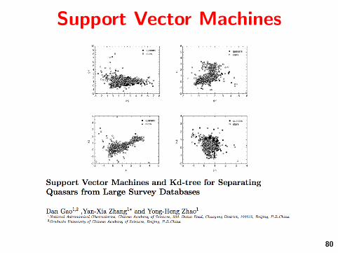
Support Vector Machines

80

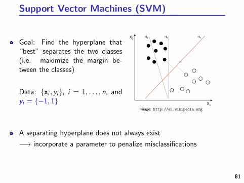
Support Vector Machines (SVM)

Goal: Find the hyperplane that“best” separates the two classes(i.e. maximize the margin be-tween the classes)

Data: {xi , yi}, i = 1, . . . , n, andyi = {−1, 1}

Image: http://en.wikipedia.org

A separating hyperplane does not always exist

−→ incorporate a parameter to penalize misclassifications

81

(Xi ·w + b)yi ≥ 1− ξi , ξi ≥ 0 for i = 1, · · · , n

minimize(1

2||w||2 + C

n∑i=1

ξi

)

ξi is capturing the degreeto which observation i ismisclassified

C is a misclassificationpenalty

Image: http://en.wikipedia.org/wiki/Support_vector_machine

82

SVM “kernel trick”

Image: http://ccforum.com/content/11/4/r83/figure/f1

83

SVM for data1 (linear) - A

R: svm(x,y,kernel = ‘‘linear’’, class.weights) in e1071 package

84

SVM for data1: fit model (linear) - A

85

SVM for data1 (linear) - B

R: svm(x,y,kernel = ‘‘linear’’, class.weights) in e1071 package

86

SVM for data1: fit model (linear) - B

87

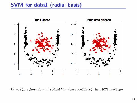
SVM for data1 (radial basis)

R: svm(x,y,kernel = ‘‘radial’’, class.weights) in e1071 package

88

SVM for data1: fit model (radial basis)

89

Classification Trees

Image: http://astronomy.swin.edu.au Image: http://dame.dsf.unina.it/dame_td.html

90

Classification trees

Goal: determine which variables are “best” at separatingobservations into the labeled groups

1 Predictor space is partitioned into hyper-rectangles

2 Any observations in the hyper-rectangle would be predicted tohave the same label

3 Next split is chosen to maximize “purity” of hyper-rectangles

Tree-based methods are not typically the best classificationmethods based on prediction accuracy, but they are often moreeasily interpreted (James et al. 2013)

CART = “Classification and Regression Trees”

91

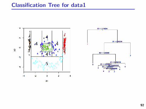
Classification Tree for data1

92

Classification Trees - recipe

Recipe

Start at the “top” of the tree and use recursive binary splitting togrow the tree

At each split, determine the classification error rate for the newregion (i.e. the number of observations that are not of the majorityclass in their region)−→ The Gini Index or cross-entropy are better for node purity.

R: tree(y ∼ x) in tree package.

93

Classification Trees - remarks

Tree pruning - the classification tree may be over fit, or toocomplex; pruning removes portions of the tree that are not usefulfor the classification goals of the tree.

Bootstrap aggregation (aka “bagging”) - there is a high variancein classification trees, and bagging (averaging over many trees)provides a means for variance reduction. (Boosting is anotherapproach, but grows trees sequentially rather using a bootstrappedsample.)

Random forest - similar idea to bagging except it incorporates astep that helps to decorrelate the trees.

94

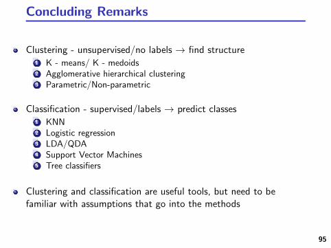
Concluding Remarks

Clustering - unsupervised/no labels → find structure1 K - means/ K - medoids2 Agglomerative hierarchical clustering3 Parametric/Non-parametric

Classification - supervised/labels → predict classes1 KNN2 Logistic regression3 LDA/QDA4 Support Vector Machines5 Tree classifiers

Clustering and classification are useful tools, but need to befamiliar with assumptions that go into the methods

95

Bibliography

Feigelson, E. D., Getman, K. V., Townsley, L. K., Broos, P. S., Povich, M. S.,Garmire, G. P., King, R. R., Montmerle, T., Preibisch, T., Smith, N., et al.(2011), “X-ray Star Clusters in the Carina Complex,” The AstrophysicalJournal Supplement Series, 194, 9.

Hastie, T., Tibshirani, R., Friedman, J., Hastie, T., Friedman, J., andTibshirani, R. (2009), The elements of statistical learning, vol. 2, Springer.

James, G., Witten, D., Hastie, T., and Tibshirani, R. (2013), An Introductionto Statistical Learning with Applications in R, vol. 1 of Springer Texts inStatistics, Springer.

Li, H.-b. and Henning, T. (2011), “The alignment of molecular cloud magneticfields with the spiral arms in M33,” Nature, 479, 499–501.

Mukherjee, S., Feigelson, E. D., Babu, G. J., Murtagh, F., Fraley, C., andRaftery, A. (1998), “Three types of gamma-ray bursts,” The AstrophysicalJournal, 508, 314.

Wasserman, L. (2004), All of statistics: a concise course in statistical inference,Springer.

96