Embed Size (px)
Citation preview
TIME-RESOLVED FLUORESCENCE
STUDIES OF PROTEIN AGGREGATION
LEADING TO AMYLOID FORMATION
BY JASON THOMAS GIURLEO
A dissertation submitted to the
Graduate School—New Brunswick
Rutgers, The State University of New Jersey
In partial fulfillment of the requirements
For the degree of
Doctor of Philosophy
Graduate Program in Chemistry and Chemical Biology
Written under the direction of
David S. Talaga
And approved by
New Brunswick, New Jersey
October, 2008
ABSTRACT OF THE DISSERTATION
Time-resolved fluorescence studies of protein
aggregation leading to amyloid formation
by Jason Thomas Giurleo
Dissertation Director: David S. Talaga
Aggregation of soluble polypeptides or proteins into insoluble amyloid fibrils con-
taining the cross-β structural motif has been observed in the progression of over
20 diseases. Self-assembly mechanisms have been proposed but are not well-
established. Recent evidence has shifted some of the focus from amyloid fibrils
to prefibrillar amyloidogenic aggregates as the cause of disease symptoms. We
used time-resolved non-covalent fluorescence labeling to follow the conformational
changes occurring in a model protein (β-lactoglobulin) during amyloid aggrega-
tion. The data was analyzed using a novel model-free globally regularized fitting
technique. This reduction of model space allowed for stable fitting and the ability
to identify intermediate species. An aggregation model was then proposed. In the
second half of this thesis, our attention is shifted to α-synuclein (αSyn). αSyn is
the majority protein component of the fibrillar inclusion bodies found in brains of
Parkinson’s disease patients. We have begun a set of fluorescence lifetime experi-
ments using covalent and non-covalent labeling schemes to elucidate the dynamic,
conformational and aggregation properties of αSyn.
ii

Acknowledgements
Acknowledgements begin with my mentor, Professor David Talaga. As a dance
instructor, he taught me my first steps of Lindy Hop, well before either of us
began here at Rutgers. As a mentor, I thank him for pushing me as hard has he
pulled for me. I would like to thank my committee: Professors Barbara Brod-
sky, Ronald Levy and Edward Castner. I would especially thank Ed for all of
the insightful conversations and for the use his laser system to take most of the
time-resolved fluorescence data presented in this dissertation. I am indebted to
Researchers Dave Remeta and Conceicao Minetti who been so generous with their
time; “helpful” is not a strong enough word. I would like to thank the Talaga
research group: Troy Messina, Jeremy Pronchik and Xianglan He. Whether di-
rectly or indirectly, each has contributed in some way to this work by selflessly
donating their time. More importantly, their sense of humor pulled me through
the frustrating moments (or HAM as we called it). The support my family was
paramount. First, Aunt Noelle and Uncle Greg for the engaging conversations, a
place to crash, and their uncanny knack for instilling confidence in my path. Sec-
ond, my girlfriend Dorothy whose emotional support has kept my mind focused
while not letting me burn out. Many of the hours spent in Starbucks writing, she
was right by my side helping in which ever way should could. Lastly, I acknowl-
edge my parents. My well-being has always been a top priority along with their
unconditional emotional support. Okay, and some financial support too ;) And to
my mom: You took on the colossal task of proofreading this dissertation without
question, just like you did 18 years ago when you helped prepare, proofread, and
type my first science project. See, it was all worth it!
iii

Chapters 2 and 3 where previously published in the The Journal of Chemical
Physics, 128:114114(118), 2008 and Journal of Molecular Biology 381:13321348,
2008, respectively. The author of this dissertation was the primary author of two
contributing publications.
iv
Dedication
Essay as part of my application to The College of New Jersey (circa February
1995):
The person who has had a significant influence in my life is Thomas Puglisi.
He is a kind, loving and patient man.
As a child my favorite place was his basement workshop where we would
conduct “Mr. Wizard”- type experiments. As I watched eagerly, he patiently
would answer my many questions, never making my inquiries seem frivolous. I
loved observing him fix things, and many times he would trust me with his tools.
He always would listen to my ideas and opinions about possible solutions. Tom
taught me problem solving by having me look at a situation from many different
angles. I learned that nothing should be overlooked, no matter how simple or
obvious. Problem solving not only became challenging, but also rewarding. I
still treasure the small, self-propelling, wooden toys we made together. Now,
after studying physics, I realized that he applied complex laws of physics to make
a simple toy! As I grew older, and several school projects later, I began to
appreciate his methodical, practical, and efficient approach to making or fixing
something. I would revel in drawing up plans with objectives and then seeing
them become a reality Tom’s gentle guidance through my trial and error process,
without criticizing me for mistakes, gave me the confidence to keep trying.
Early on, Tom Puglisi sparked a curiosity in me about the complex worlds
of chemistry and physics. He taught me that patience, determination, creativity,
and imagination are the keys to a successful outcome. I am proud to say that the
man who has significantly influenced my life and my desire to become a scientist
v

is my grandfather, Thomas Puglisi.
Tom (1917-2002) was a chemist for Hoffmann-LaRoche for 43 years includ-
ing a three year hiatus serving as an Army Sargent, stationed on the European
front under General Patton. Tom passed away from complications of Alzheimer’s
disease, and is to whom I humbly dedicate this work.
vi

Table of Contents
Abstract . . . . . . . . . . . . . . . . . . . . . . . . . . . . . . . . . . . . ii
Acknowledgements . . . . . . . . . . . . . . . . . . . . . . . . . . . . . iii
Dedication . . . . . . . . . . . . . . . . . . . . . . . . . . . . . . . . . . . v
List of Tables . . . . . . . . . . . . . . . . . . . . . . . . . . . . . . . . . xv
List of Figures . . . . . . . . . . . . . . . . . . . . . . . . . . . . . . . . xvi
1. Introduction . . . . . . . . . . . . . . . . . . . . . . . . . . . . . . . . 1
Personal motivation . . . . . . . . . . . . . . . . . . . . . . 1
Disease . . . . . . . . . . . . . . . . . . . . . . . . . . . . . 1
β-Lactoglobulin studies . . . . . . . . . . . . . . . . . . . . 5
Using global probabilistic constraints to develop global mod-
els . . . . . . . . . . . . . . . . . . . . . . . . . . 8
β-LGa revisited, model solidified . . . . . . . . . . . . . . 8
Spectroscopic studies of covalently labeled αSyn . . . . . . 9
Aggregation studies of αSyn . . . . . . . . . . . . . . . . . 10
References . . . . . . . . . . . . . . . . . . . . . . . . . . . . . . . . . . . 12
2. Global fitting without a global model: regularization based on
the continuity of the evolution of parameter distributions. . . . . 14
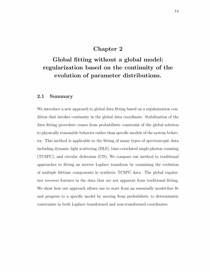
2.1. Summary . . . . . . . . . . . . . . . . . . . . . . . . . . . . . . . 14
2.2. Introduction . . . . . . . . . . . . . . . . . . . . . . . . . . . . . . 15
2.3. Methods . . . . . . . . . . . . . . . . . . . . . . . . . . . . . . . . 22
vii

2.3.1. IPG Regularizer . . . . . . . . . . . . . . . . . . . . . . . . 22
Locally Regularized IPG . . . . . . . . . . . . . . . . . . . 23
Globally Regularized IPG . . . . . . . . . . . . . . . . . . 24
2.3.2. Data Simulations . . . . . . . . . . . . . . . . . . . . . . . 25
2.3.3. Fitting Mechanics . . . . . . . . . . . . . . . . . . . . . . . 26
Levenberg-Marquardt . . . . . . . . . . . . . . . . . . . . . 27
Active-Set and Interior Point Gradient . . . . . . . . . . . 28
Maximum Entropy method fits . . . . . . . . . . . . . . . 29
2.3.4. Model Similarity Criteria . . . . . . . . . . . . . . . . . . . 30
Quality-of-fit . . . . . . . . . . . . . . . . . . . . . . . . . 30
Quality-of-Parameters . . . . . . . . . . . . . . . . . . . . 31
2.3.5. Error Estimates . . . . . . . . . . . . . . . . . . . . . . . . 32
2.4. Results . . . . . . . . . . . . . . . . . . . . . . . . . . . . . . . . . 33
2.4.1. Levenberg-Marquardt . . . . . . . . . . . . . . . . . . . . 33
Three-Exponential Model Fits . . . . . . . . . . . . . . . . 34
Four-Exponential Model Fits . . . . . . . . . . . . . . . . 36
2.4.2. Active-Set . . . . . . . . . . . . . . . . . . . . . . . . . . . 38
2.4.3. Maximum Entropy Method . . . . . . . . . . . . . . . . . 40
2.4.4. Interior Point Gradient Method . . . . . . . . . . . . . . . 40
Unregularized IPG . . . . . . . . . . . . . . . . . . . . . . 42
Locally Regularized IPG . . . . . . . . . . . . . . . . . . . 43
Globally Regularized IPG . . . . . . . . . . . . . . . . . . 45
2.4.5. Global Model LM . . . . . . . . . . . . . . . . . . . . . . . 48
Traditional Global Model LM . . . . . . . . . . . . . . . . 49
Regularized Global Model LM . . . . . . . . . . . . . . . . 52
2.5. Discussion . . . . . . . . . . . . . . . . . . . . . . . . . . . . . . . 53
2.5.1. Comparison of Methods . . . . . . . . . . . . . . . . . . . 53
viii

Reduced Chi-square . . . . . . . . . . . . . . . . . . . . . 53
Kullback-Liebler divergence . . . . . . . . . . . . . . . . . 54
Population Evolution . . . . . . . . . . . . . . . . . . . . . 59
2.5.2. Prior Knowledge and Probabilistic Constraints . . . . . . . 59
2.5.3. Global fitting strategy . . . . . . . . . . . . . . . . . . . . 61
2.6. Conclusions . . . . . . . . . . . . . . . . . . . . . . . . . . . . . . 64
References . . . . . . . . . . . . . . . . . . . . . . . . . . . . . . . . . . . 65
3. β-Lactoglobulin Assembles into Amyloid through Sequential Ag-
gregated Intermediates . . . . . . . . . . . . . . . . . . . . . . . . . . . 69
3.1. Summary . . . . . . . . . . . . . . . . . . . . . . . . . . . . . . . 69
3.2. Introduction . . . . . . . . . . . . . . . . . . . . . . . . . . . . . . 70
3.2.1. Amyloid Formation . . . . . . . . . . . . . . . . . . . . . . 70
3.2.2. Bovine β-lactoglobulin variant A . . . . . . . . . . . . . . 72
3.2.3. Biophysical Approaches to Aggregation . . . . . . . . . . . 74
3.3. Results . . . . . . . . . . . . . . . . . . . . . . . . . . . . . . . . . 76
3.3.1. AFM shows sequential growth of aggregates . . . . . . . . 76
3.3.2. DLS resolves early lag phase aggregation . . . . . . . . . . 77
Interpretation . . . . . . . . . . . . . . . . . . . . . . . . . 78
3.3.3. ThT tracks structural conversions . . . . . . . . . . . . . . 78
3.3.4. ANS reports changes in hydrophobic regions and calyx loss. 82
ANS aggregation reversibility assay . . . . . . . . . . . . . 90
3.4. Discussion . . . . . . . . . . . . . . . . . . . . . . . . . . . . . . . 92
3.4.1. Conformationally lability prior to incubation . . . . . . . . 92
3.4.2. Early lag phase aggregation was more reversible . . . . . . 94
3.4.3. Late lag phase aggregation loses calyx . . . . . . . . . . . 95
3.4.4. Protofibrils appeared after day 20 . . . . . . . . . . . . . . 96
ix
3.4.5. Overall mechanism . . . . . . . . . . . . . . . . . . . . . . 97
3.5. Materials and Methods . . . . . . . . . . . . . . . . . . . . . . . . 100
3.5.1. Materials . . . . . . . . . . . . . . . . . . . . . . . . . . . 100
3.5.2. β-LGa incubations . . . . . . . . . . . . . . . . . . . . . . 100
3.5.3. Time-resolved luminescence . . . . . . . . . . . . . . . . . 101
3.5.4. Dynamic light scattering . . . . . . . . . . . . . . . . . . . 103
3.5.5. Atomic force microscopy . . . . . . . . . . . . . . . . . . . 105
3.6. Acknowledgments . . . . . . . . . . . . . . . . . . . . . . . . . . . 105
References . . . . . . . . . . . . . . . . . . . . . . . . . . . . . . . . . . . 106
4. Exploring αSyn with covalently attached fluorophores using time-
resolved and single molecule imaging spectroscopy . . . . . . . . . 113
4.1. Summary . . . . . . . . . . . . . . . . . . . . . . . . . . . . . . . 113
4.2. Introduction . . . . . . . . . . . . . . . . . . . . . . . . . . . . . . 114
4.3. Methods . . . . . . . . . . . . . . . . . . . . . . . . . . . . . . . . 117
4.3.1. Selected materials . . . . . . . . . . . . . . . . . . . . . . . 117
Protein Preparation . . . . . . . . . . . . . . . . . . . . . . 117
4.3.2. Protein conjugation . . . . . . . . . . . . . . . . . . . . . . 118
4.3.3. Cysteine conjugation . . . . . . . . . . . . . . . . . . . . . 118
4.3.4. Fluorescence spectroscopy . . . . . . . . . . . . . . . . . . 118
Time-resolved fluorescence . . . . . . . . . . . . . . . . . . 119
Single molecule imaging . . . . . . . . . . . . . . . . . . . 119
4.3.5. Data analysis . . . . . . . . . . . . . . . . . . . . . . . . . 120
4.4. Results and Discussion . . . . . . . . . . . . . . . . . . . . . . . . 120
4.4.1. Properties of Alexa 488 . . . . . . . . . . . . . . . . . . . . 120
Interpretation . . . . . . . . . . . . . . . . . . . . . . . . . 122
4.4.2. Properties of Atto 590 . . . . . . . . . . . . . . . . . . . . 123
x

Interpretation . . . . . . . . . . . . . . . . . . . . . . . . . 123
4.4.3. Properties of NR-αSyn . . . . . . . . . . . . . . . . . . . 124
Interpretation . . . . . . . . . . . . . . . . . . . . . . . . . 125
4.4.4. SM . . . . . . . . . . . . . . . . . . . . . . . . . . . . . . . 128
Interpretation . . . . . . . . . . . . . . . . . . . . . . . . . 128
4.5. Conclusions . . . . . . . . . . . . . . . . . . . . . . . . . . . . . . 130
References . . . . . . . . . . . . . . . . . . . . . . . . . . . . . . . . . . . 131
5. Thermodynamic studies of α-synuclein . . . . . . . . . . . . . . . 133
5.1. Summary . . . . . . . . . . . . . . . . . . . . . . . . . . . . . . . 133
5.2. Introduction . . . . . . . . . . . . . . . . . . . . . . . . . . . . . . 133
Disease . . . . . . . . . . . . . . . . . . . . . . . . . . . . . 133
Intrinsically disordered protein . . . . . . . . . . . . . . . . 134
Two thermodynamic states . . . . . . . . . . . . . . . . . 135
5.3. Methods . . . . . . . . . . . . . . . . . . . . . . . . . . . . . . . . 136
5.3.1. Preparation and Purification . . . . . . . . . . . . . . . . . 136
5.3.2. UV . . . . . . . . . . . . . . . . . . . . . . . . . . . . . . . 136
5.3.3. DLS . . . . . . . . . . . . . . . . . . . . . . . . . . . . . . 137
5.3.4. CD . . . . . . . . . . . . . . . . . . . . . . . . . . . . . . . 138
5.3.5. Two-state model . . . . . . . . . . . . . . . . . . . . . . . 139
5.4. Results . . . . . . . . . . . . . . . . . . . . . . . . . . . . . . . . . 140
5.4.1. UV . . . . . . . . . . . . . . . . . . . . . . . . . . . . . . . 140
5.4.2. Circular Dichroism . . . . . . . . . . . . . . . . . . . . . . 141
5.4.3. Dynamic Light Scattering . . . . . . . . . . . . . . . . . . 143
5.5. Discussion . . . . . . . . . . . . . . . . . . . . . . . . . . . . . . . 144
5.5.1. Future studies . . . . . . . . . . . . . . . . . . . . . . . . . 146
5.6. Conclusions . . . . . . . . . . . . . . . . . . . . . . . . . . . . . . 147
xi
References . . . . . . . . . . . . . . . . . . . . . . . . . . . . . . . . . . . 148
6. Aggregation methods of α-synuclein. . . . . . . . . . . . . . . . . 151
6.1. Summary . . . . . . . . . . . . . . . . . . . . . . . . . . . . . . . 151
6.2. Introduction . . . . . . . . . . . . . . . . . . . . . . . . . . . . . . 151
Mechanism and amyloid formation. . . . . . . . . . . . . . 151
Incubation conditions affect aggregation rates. . . . . . . . 153
Experimental design . . . . . . . . . . . . . . . . . . . . . 153
6.3. Methods . . . . . . . . . . . . . . . . . . . . . . . . . . . . . . . . 155
Chemicals . . . . . . . . . . . . . . . . . . . . . . . . . . . 155
Protein Preparation . . . . . . . . . . . . . . . . . . . . . . 155
Sample preparation for time-zero Native Gel . . . . . . . . 155
Sample preparation for incubation . . . . . . . . . . . . . . 157
ThioflavinT assay . . . . . . . . . . . . . . . . . . . . . . . 158
DLS and SLS assay . . . . . . . . . . . . . . . . . . . . . . 159
AFM . . . . . . . . . . . . . . . . . . . . . . . . . . . . . . 160
Native gel electrophoresis . . . . . . . . . . . . . . . . . . 160
Photograph of final product . . . . . . . . . . . . . . . . . 160
6.4. Results . . . . . . . . . . . . . . . . . . . . . . . . . . . . . . . . . 160
6.4.1. Initial conditions . . . . . . . . . . . . . . . . . . . . . . . 160
6.4.2. Final product - Visual Inspection and AFM . . . . . . . . 162
6.4.3. SS ThT Assay . . . . . . . . . . . . . . . . . . . . . . . . . 163
6.4.4. SLS . . . . . . . . . . . . . . . . . . . . . . . . . . . . . . 165
6.4.5. Dynamic Light Scattering . . . . . . . . . . . . . . . . . . 167
6.4.6. Time-Resolved ThT luminescence . . . . . . . . . . . . . . 170
6.4.7. Data recapitulation . . . . . . . . . . . . . . . . . . . . . . 172
FS . . . . . . . . . . . . . . . . . . . . . . . . . . . . . . . 172
xii

US . . . . . . . . . . . . . . . . . . . . . . . . . . . . . . . 172
UR . . . . . . . . . . . . . . . . . . . . . . . . . . . . . . . 173
6.5. Discussion . . . . . . . . . . . . . . . . . . . . . . . . . . . . . . . 174
Differences in methods . . . . . . . . . . . . . . . . . . . . 174
6.5.1. Preparation Effects . . . . . . . . . . . . . . . . . . . . . . 174
6.5.2. Agitation Effects . . . . . . . . . . . . . . . . . . . . . . . 175
6.5.3. Mechanistic consequences . . . . . . . . . . . . . . . . . . 177
Shaking versus rotating . . . . . . . . . . . . . . . . . . . . 177
6.5.4. Biological relevance of in vitro agitation studies . . . . . . 178
6.5.5. Future experiments . . . . . . . . . . . . . . . . . . . . . . 179
Teflon beads - No head space - Rotated . . . . . . . . . . . 179
Quiescent- No head space - Filtered . . . . . . . . . . . . . 179
Elucidating intermediate species with TRF studies covalently-
labeled αSN. . . . . . . . . . . . . . . . . . . . . 180
FRET study of the co-incubation of two different αSN con-
jugates . . . . . . . . . . . . . . . . . . . . . . . . 180
6.6. Conclusions . . . . . . . . . . . . . . . . . . . . . . . . . . . . . . 181
References . . . . . . . . . . . . . . . . . . . . . . . . . . . . . . . . . . . 182
7. Supplementary Materials . . . . . . . . . . . . . . . . . . . . . . . . 185
7.1. Summary . . . . . . . . . . . . . . . . . . . . . . . . . . . . . . . 185
7.2. Simulating DLS data . . . . . . . . . . . . . . . . . . . . . . . . . 185
7.2.1. Generating DLS data, IGOR code . . . . . . . . . . . . . . 187
7.3. γ-cyclodextrin (γ-CD) . . . . . . . . . . . . . . . . . . . . . . . . 190
7.4. Urea titration of β-LGa . . . . . . . . . . . . . . . . . . . . . . . 192
References . . . . . . . . . . . . . . . . . . . . . . . . . . . . . . . . . . . 194
8. Explanation of Global Regularization Code . . . . . . . . . . . . 195
xiii

8.1. Summary . . . . . . . . . . . . . . . . . . . . . . . . . . . . . . . 195
8.2. Introduction . . . . . . . . . . . . . . . . . . . . . . . . . . . . . . 195
8.2.1. Fast GIPG . . . . . . . . . . . . . . . . . . . . . . . . . . . 198
8.3. Flow charts . . . . . . . . . . . . . . . . . . . . . . . . . . . . . . 202
References . . . . . . . . . . . . . . . . . . . . . . . . . . . . . . . . . . . 208
9. Globally regularized interior point gradient method, Igor code 209
Vita . . . . . . . . . . . . . . . . . . . . . . . . . . . . . . . . . . . . . . . 311
xiv

List of Tables
4.1. Physical properties and other information concerning Alexa 488
and Atto 590. τ is the lifetime, τn is the calculated natural life-
time, CF280 is the correction factor at 280 nm, or A280 divided
by the absorption at maximum, CF260 is the same as CF280 but
at A280, εmax extinction coefficient, λ is wavelength at absorption
maximum, A493 is relative to the Atto absorption at 493 nm. . . . 116
5.1. Table of fit parameters and Tm for spectroscopic fit. Fit parameters
are described in the text. Tm is calculate from Eq. 5.5. O0′ and
O1′ are used for the global fitting of 198 and 222 nm CD data. The
observables (O) are in units of the measurement, γ is dimensionless,
and ε is in Joules. . . . . . . . . . . . . . . . . . . . . . . . . . . . 144
6.1. A select list publications concerning aggregation of αSN. Time to
the beginning of the growth phase is dependent on preparation of
monomer protein and agitation conditions. All incubations in this
list carried out at 37 C. . . . . . . . . . . . . . . . . . . . . . . . 156
xv

List of Figures
1.1. Classic sigmoidal kinetics of amyloid fibrils in vitro. Left panel:
The canonical explanation of amyloid growth has been proposed
from histological staining assays in vitro. The explanation involves
three phases: lag, growth and elongation. Right panel: Adding
pre-formed seeds eliminates the lag phase. [17] See Fig. 1.2 for a
comprehensive description of the possible intermediates that have
been proposed. . . . . . . . . . . . . . . . . . . . . . . . . . . . . 3
xvi

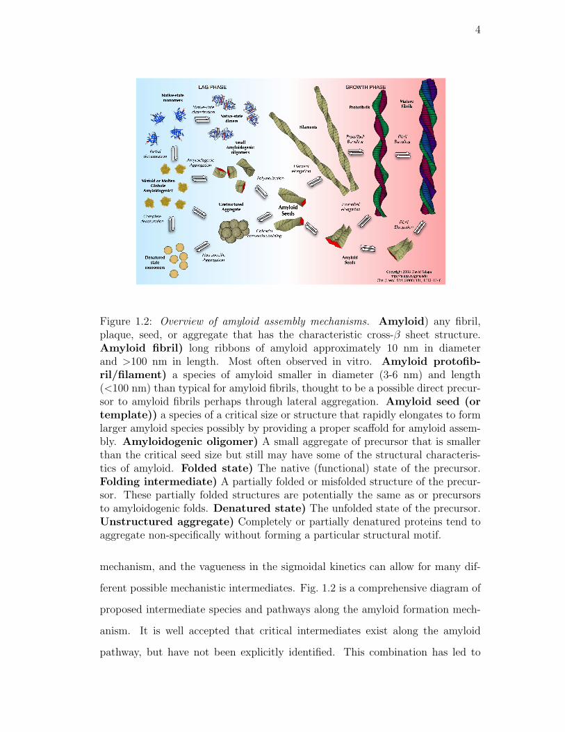
1.2. Overview of amyloid assembly mechanisms. Amyloid) any fib-
ril, plaque, seed, or aggregate that has the characteristic cross-β
sheet structure. Amyloid fibril) long ribbons of amyloid approx-
imately 10 nm in diameter and >100 nm in length. Most often
observed in vitro. Amyloid protofibril/filament) a species of
amyloid smaller in diameter (3-6 nm) and length (<100 nm) than
typical for amyloid fibrils, thought to be a possible direct precursor
to amyloid fibrils perhaps through lateral aggregation. Amyloid
seed (or template)) a species of a critical size or structure that
rapidly elongates to form larger amyloid species possibly by pro-
viding a proper scaffold for amyloid assembly. Amyloidogenic
oligomer) A small aggregate of precursor that is smaller than
the critical seed size but still may have some of the structural
characteristics of amyloid. Folded state) The native (functional)
state of the precursor. Folding intermediate) A partially folded
or misfolded structure of the precursor. These partially folded
structures are potentially the same as or precursors to amyloido-
genic folds. Denatured state) The unfolded state of the pre-
cursor. Unstructured aggregate) Completely or partially dena-
tured proteins tend to aggregate non-specifically without forming
a particular structural motif. . . . . . . . . . . . . . . . . . . . . . 4
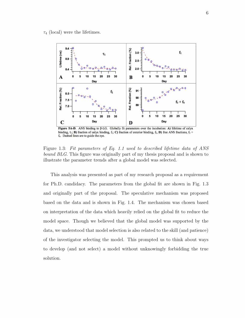
1.3. Fit parameters of Eq. 1.1 used to described lifetime data of ANS
bound BLG. This figure was originally part of my thesis proposal
and is shown to illustrate the parameter trends after a global model
was selected. . . . . . . . . . . . . . . . . . . . . . . . . . . . . . . 6
xvii

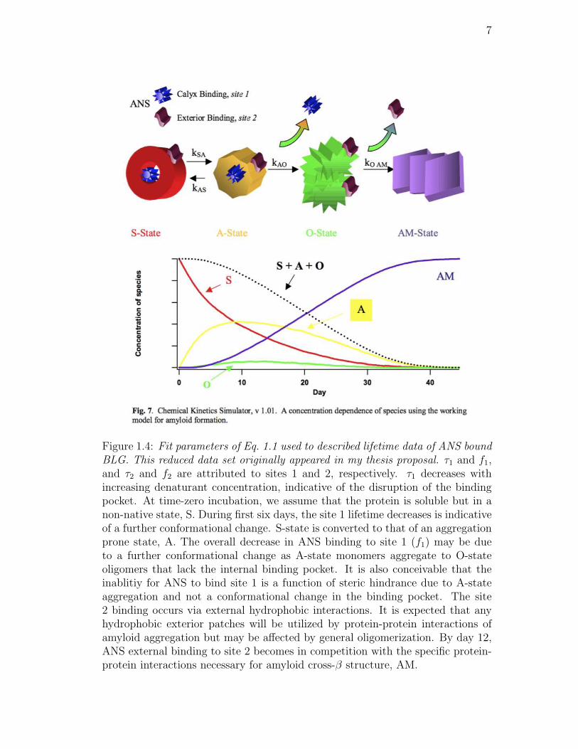
1.4. Fit parameters of Eq. 1.1 used to described lifetime data of ANS
bound BLG. This reduced data set originally appeared in my thesis
proposal. τ1 and f1, and τ2 and f2 are attributed to sites 1 and 2, re-
spectively. τ1 decreases with increasing denaturant concentration,
indicative of the disruption of the binding pocket. At time-zero
incubation, we assume that the protein is soluble but in a non-
native state, S. During first six days, the site 1 lifetime decreases is
indicative of a further conformational change. S-state is converted
to that of an aggregation prone state, A. The overall decrease in
ANS binding to site 1 (f1) may be due to a further conformational
change as A-state monomers aggregate to O-state oligomers that
lack the internal binding pocket. It is also conceivable that the
inablitiy for ANS to bind site 1 is a function of steric hindrance
due to A-state aggregation and not a conformational change in the
binding pocket. The site 2 binding occurs via external hydrophobic
interactions. It is expected that any hydrophobic exterior patches
will be utilized by protein-protein interactions of amyloid aggrega-
tion but may be affected by general oligomerization. By day 12,
ANS external binding to site 2 becomes in competition with the
specific protein-protein interactions necessary for amyloid cross-β
structure, AM. . . . . . . . . . . . . . . . . . . . . . . . . . . . . 7
xviii
2.1. Experimental prior knowledge With global fitting available, prior
knowledge in the form of a regularizer can either be be applied in
the Laplace transform dimension, k, or in the experimental evolu-
tion dimension, y. In the left panel the individual data transients
are indicated by the black mesh lines. In the right panels, the direc-
tion of continuity conditions is indicated by the black mesh lines.
The top right panel emphasizes the continuity in the k dimension
implying continuous distributions of properties. The bottom right
panel emphasizes continuity in the y dimension implying continu-
ous evolution of population. . . . . . . . . . . . . . . . . . . . . . 18
2.2. f(k, y) for three exponential fits. Starting from top panel down:
exemplar solution parameters, fit solution parameters synthesized
with I = 105, 104, 103, 200 peak mean photons. Superimposed
numbers correspond to species described in Methods. . . . . . . . 34
2.3. f(k, y) for four exponential fits. Panels are described in figure 2.2. 36
2.4. f(k, y) for Active-Set Method fits. Panels are described in figure 2.2. 39
2.5. f(k, y) for MEM fits. Panels are described in figure 2.2. . . . . . . 41
2.6. f(k, y) for IPG fits. Panels are described in figure 2.2. . . . . . . 42
2.7. f(k, y)for Locally Regularized IPG fits. Panels are described in
figure 2.2. . . . . . . . . . . . . . . . . . . . . . . . . . . . . . . . 44
2.8. f(k, y) for Globally Regularized IPG fits. Panels are described in
figure 2.2. . . . . . . . . . . . . . . . . . . . . . . . . . . . . . . . 46
2.9. f(k, y) for Global Model fits. Panels are described in figure 2.2. . . 49
2.10. f(k, y) for Regularized Global Model fits. Panels are described in
Fig. 2.2. . . . . . . . . . . . . . . . . . . . . . . . . . . . . . . . . 51
xix
2.11. χ2r for all I using different fitting methods. (4)–Three Exponential
fits, ()–Four Exponential fits, ()–Active-Set Method fits, (./)–
Maximum Entropy Method fits, (•)–IPG fits, (⊗)–Locally Reg-
ularized IPG fits, ()–Globally Regularized IPG fits, (+)–Global
Model fits, (∗)–Regularized Global Model fits. . . . . . . . . . . . 55
2.12. Kullback-Liebler divergence from the exemplar model versus I us-
ing the different fitting methods. Fitting methods are represented
in the same markers as in Fig. 2.11. . . . . . . . . . . . . . . . . . 56
2.13. POP for all I using different fitting methods. Fitting methods are
represented in the same markers as in Fig. 2.11. . . . . . . . . . . 57
2.14. Species Populations, Si, at I = 104). Species 1 through 4 are
represented by brown©, green ♦, blue 4, and red respectively.
The solid lines of the same respective color, represent the exemplar
species populations, Si. . . . . . . . . . . . . . . . . . . . . . . . . 58
2.15. Model selection vs model discovery Current paradigm of global
analysis follows the thin solid lines. In this case, a model is se-
lected first with deterministic constraints a priori,the quality-of-fit
is evaluated and a new model is chosen if necessary. Following the
double lines, we propose using globally regularized method to dis-
cover the model of the evolution of the system based on the data
and prior knowledge. Once a model is discovered, deterministic
constraints can be applied in order to reach conclusions about the
underlying physical system. . . . . . . . . . . . . . . . . . . . . . 62
xx
3.1. The possible binding sites of ANS to β-LGa. Hydrophobic amino
acid residues are colored in slate, hydrophilic residues in brick.
ANS was docked to β-LGa using PyMOL, and minimized using
molecular mechanics software IMPACT.[86] The left panel is a 16 A
slab of the van der Waals surface without secondary structure to
illustrate the binding of ANS in the hydrophobic calyx site (A).
The right panel is rotated 90 about vertical axis of left panel to
show the postulated intercalation site in the hydrophobic region
between the main α-helix and β-barrel surface patch (B). Roughly
two-thirds of the calyx volume is represented by its “mouth” and
may be considered to be a third ANS binding site (C). . . . . . . 72
3.2. AFM images of β-LGa aggregation under amyloidogenic condi-
tions. Days 10, 22, 29, and 65 are shown as labeled. Images are col-
ored by height and approximately correspond to species described
in the text. AFM heights are uncorrected for tip penetration of the
soft samples. Prior to day 10, there was little indication of stable
aggregates adhering to amino-silanized mica surface. The first sign
of small stable oligomers (shown in green) appear at day 10. The
total number and aspect ratio of the aggregates increases through
day 22. After four weeks, small protofibillar species are apparent
and range from 50 to several hundred nanometers in length. Fib-
rillar species ranging in height and length dominate at two months
of incubation. Large amorphous aggregates appear as early as day
10, but appear to be off the amyloid formation pathway. . . . . . 74
xxi
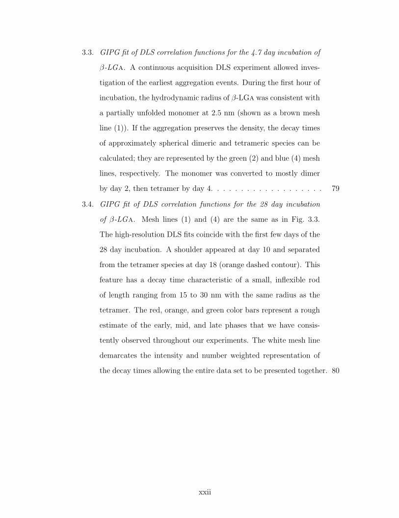
3.3. GIPG fit of DLS correlation functions for the 4.7 day incubation of
β-LGa. A continuous acquisition DLS experiment allowed inves-
tigation of the earliest aggregation events. During the first hour of
incubation, the hydrodynamic radius of β-LGa was consistent with
a partially unfolded monomer at 2.5 nm (shown as a brown mesh
line (1)). If the aggregation preserves the density, the decay times
of approximately spherical dimeric and tetrameric species can be
calculated; they are represented by the green (2) and blue (4) mesh
lines, respectively. The monomer was converted to mostly dimer
by day 2, then tetramer by day 4. . . . . . . . . . . . . . . . . . . 79
3.4. GIPG fit of DLS correlation functions for the 28 day incubation
of β-LGa. Mesh lines (1) and (4) are the same as in Fig. 3.3.
The high-resolution DLS fits coincide with the first few days of the
28 day incubation. A shoulder appeared at day 10 and separated
from the tetramer species at day 18 (orange dashed contour). This
feature has a decay time characteristic of a small, inflexible rod
of length ranging from 15 to 30 nm with the same radius as the
tetramer. The red, orange, and green color bars represent a rough
estimate of the early, mid, and late phases that we have consis-
tently observed throughout our experiments. The white mesh line
demarcates the intensity and number weighted representation of
the decay times allowing the entire data set to be presented together. 80
xxii

3.5. GIPG fit of ThT luminescence decays in the presence of β-LGa
over a 28 day incubation. Left panel: The evolution of lifetime
distributions show the onset of luminescent species occurs in stages.
The reduced chi-squared (χ2r) for this global fit was 1.022. Right
panel: Incubation time slices of ThT lifetime distributions with
different contributions at days 0, 5, 16, 32 and 65 are as labeled
and correspond to the dotted mesh lines in the right panel. To
depict the growth and loss of different luminescence components
along the incubation timecourse, the distributions are filled to the
baseline with colors corresponding to the trace where the particular
component dominates. For example the green filling matches the
peaks at day 32, but the same components are less prevalent at
day 16. . . . . . . . . . . . . . . . . . . . . . . . . . . . . . . . . . 81
3.6. GIPG fit of ANS fluorescence decays in the presence of β-LGa
over a 28 day incubation. The χ2r for this global fit was 1.019. The
distribution of fluorescence lifetimes showed the variety of binding
environments for ANS and their systematic population changes
changes with incubation time. The reduction of some peaks (i.e.
a, b and c) and the increase of others (i.e. g, h, i) reflected the
conformational changes experienced by β-LGa as it assembles into
fibrils. All peaks are assigned to different ANS environments in
the text. This model-free fit was used as the basis for further data
reduction as described in the text and shown in Fig. 3.7. . . . . . 83
xxiii
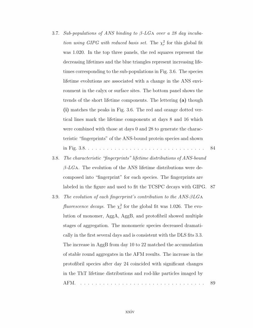
3.7. Sub-populations of ANS binding to β-LGa over a 28 day incuba-
tion using GIPG with reduced basis set. The χ2r for this global fit
was 1.020. In the top three panels, the red squares represent the
decreasing lifetimes and the blue triangles represent increasing life-
times corresponding to the sub-populations in Fig. 3.6. The species
lifetime evolutions are associated with a change in the ANS envi-
ronment in the calyx or surface sites. The bottom panel shows the
trends of the short lifetime components. The lettering (a) though
(i) matches the peaks in Fig. 3.6. The red and orange dotted ver-
tical lines mark the lifetime components at days 8 and 16 which
were combined with those at days 0 and 28 to generate the charac-
teristic “fingerprints” of the ANS-bound protein species and shown
in Fig. 3.8. . . . . . . . . . . . . . . . . . . . . . . . . . . . . . . . 84
3.8. The characteristic “fingerprints” lifetime distributions of ANS-bound
β-LGa. The evolution of the ANS lifetime distributions were de-
composed into “fingerprint” for each species. The fingerprints are
labeled in the figure and used to fit the TCSPC decays with GIPG. 87
3.9. The evolution of each fingerprint’s contribution to the ANS-βLGa
fluorescence decays. The χ2r for the global fit was 1.026. The evo-
lution of monomer, AggA, AggB, and protofibril showed multiple
stages of aggregation. The monomeric species decreased dramati-
cally in the first several days and is consistent with the DLS fits 3.3.
The increase in AggB from day 10 to 22 matched the accumulation
of stable round aggregates in the AFM results. The increase in the
protofibril species after day 24 coincided with significant changes
in the ThT lifetime distributions and rod-like particles imaged by
AFM. . . . . . . . . . . . . . . . . . . . . . . . . . . . . . . . . . 89
xxiv

3.10. GIPG fit for the ANS reversibility assay The stability of the monomer
and aggregate species are evaluated by reintroducing the incubated
sample to a low urea condition. Yellow mesh lines demarcate 3.6,
4.3, 13, and 16 ns to emphasized the loss gain of species more
clearly. The most dramatic feature is the nearly 50% loss of the
16 ns species, presumably the calyx-bound ANS, by day 8. The
loss contemporaneously matches the change over of the 4.3 to the
3.6 ns species. The χ2r for the global fit was 1.002. . . . . . . . . . 90
3.11. Proposed mechanism of β lactoglobulin A aggregation. Amyloido-
genic conditions put βLGa into a disordered, conformationally la-
bile state that reversibly aggregates into dimers and tetramers that
are stabilized in part by hydrophobic interactions. The calyx is in-
tact but structurally altered. As aggregation continues, the calyx
is lost and the loosely associated oligomers convert to higher or-
der, more stable aggregates. These aggregates then convert into
protofibrils that elongate in the classic growth phase of sigmoidal
kinetics. Monomeric: The top is the folded monomer, the mid-
dle was obtained by modeling the unfolding of the the C-terminal
α-helix and β-strand I. The bottom was obtained by flattening the
barrel into a sheet. Aggregate A: These oligomers were obtained
by aligning complementary surfaces of the middle monomer struc-
ture. Aggregate B: This octamer was modeled by stacking the
flattened monomer structure into four layers. Protofibrils: Four
sheets of the canonical cross-β structure. . . . . . . . . . . . . . . 93
4.1. The number of publications between the years 1962 to 2007, with the
concepts of fluorescence, lifetimes and protein. The importance of
time-resolved fluorescence has grown substantially in recent years.
Information was provided by the Chemical Abstract Service. . . . 114
xxv

4.2. Structures of the fluorophores featured in this chapter. A) Alexa
Fluor 488, B) Atto 590 and C) Nile Red. . . . . . . . . . . . . . . 117
4.3. Steady-state emission spectra versus temperature. Left panel: steady-
state emission at the start, middle and end of temperature cycle.
The spectrum exhibits typical thermal broadening at high temper-
atures, but is reversible after the completion of the cycle. Right
panel: a contour plot of the evolving emission spectra across the
temperature cycle. There is slight loss of signal as the sample re-
turns to back 5 C and suggests irreversible fluorescence quenching. 120
4.4. Lifetime dependence of temperature of Alexa-αSyn conjugate. The
main 4.1-ns component does not shift with temperature, but there
is a small contribution from a 800-ps species that appears as the
temperature increases. Both features are marked with circles and
will be referred to later in the text when describing the Alexa-αSyn
conjugate lifetime evolution. Reduced chi-square of the fit is 1.19. 121
4.5. Lifetime dependence of temperature of Alexa-αSyn conjugate. Two
new features, marked by squares at 1.1 and 3.4 ns appear as the
temperature increases. The Alexa-cys control is marked by circles.
Reduced chi-square of the fit is 1.11. . . . . . . . . . . . . . . . . 122
4.6. Lifetime dependence of wavelength of Atto-αSyn conjugate at 37 C.
As the temperature increases, we expect a slight shift to shorter
lifetimes as potential pathways out of the excited state increase.
Reduced chi-square is 1.17 . . . . . . . . . . . . . . . . . . . . . . 123
4.7. Absorption and emission spectra for Alexa 488 and Atto 590. . . . 124
xxvi
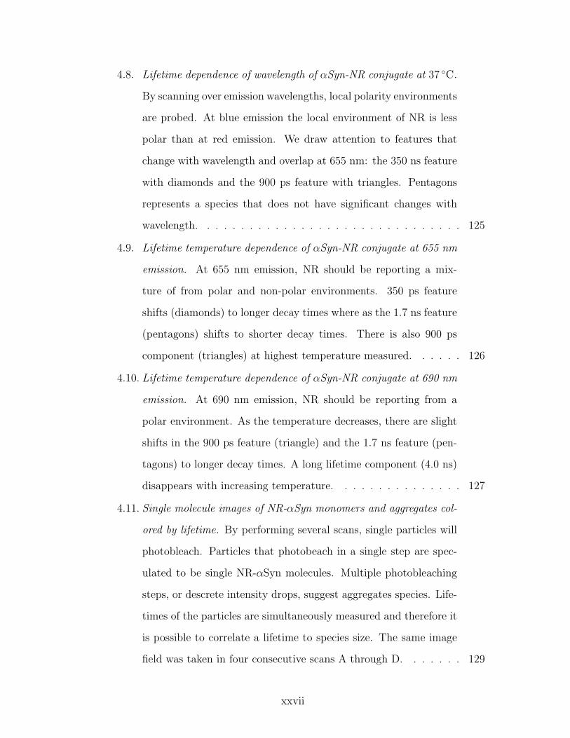
4.8. Lifetime dependence of wavelength of αSyn-NR conjugate at 37 C.
By scanning over emission wavelengths, local polarity environments
are probed. At blue emission the local environment of NR is less
polar than at red emission. We draw attention to features that
change with wavelength and overlap at 655 nm: the 350 ns feature
with diamonds and the 900 ps feature with triangles. Pentagons
represents a species that does not have significant changes with
wavelength. . . . . . . . . . . . . . . . . . . . . . . . . . . . . . . 125
4.9. Lifetime temperature dependence of αSyn-NR conjugate at 655 nm
emission. At 655 nm emission, NR should be reporting a mix-
ture of from polar and non-polar environments. 350 ps feature
shifts (diamonds) to longer decay times where as the 1.7 ns feature
(pentagons) shifts to shorter decay times. There is also 900 ps
component (triangles) at highest temperature measured. . . . . . 126
4.10. Lifetime temperature dependence of αSyn-NR conjugate at 690 nm
emission. At 690 nm emission, NR should be reporting from a
polar environment. As the temperature decreases, there are slight
shifts in the 900 ps feature (triangle) and the 1.7 ns feature (pen-
tagons) to longer decay times. A long lifetime component (4.0 ns)
disappears with increasing temperature. . . . . . . . . . . . . . . 127
4.11. Single molecule images of NR-αSyn monomers and aggregates col-
ored by lifetime. By performing several scans, single particles will
photobleach. Particles that photobeach in a single step are spec-
ulated to be single NR-αSyn molecules. Multiple photobleaching
steps, or descrete intensity drops, suggest aggregates species. Life-
times of the particles are simultaneously measured and therefore it
is possible to correlate a lifetime to species size. The same image
field was taken in four consecutive scans A through D. . . . . . . 129
xxvii

4.12. An αSyn fibril with covalently attached NR. The lifetime of a fibril
is very short compared to the monomeric conjugate. . . . . . . . . 130
5.1. Temperature dependent absorption spectra of αSyn The spectra of
αSyn at 0 C (blue), 100 C (red), and the difference spectra (ma-
genta) is also shown in the inset. Note that the peak maximum at
278 nm has not shifted with temperature. . . . . . . . . . . . . . 141
5.2. Fit to the absorption evolution at 287 nm of αSyn versus temper-
ature. In the bottom graph, data is represented by the red circles
and the fit line is in blue. The residuals are plotted in the top
graph in red circles. . . . . . . . . . . . . . . . . . . . . . . . . . . 142
5.3. CD spectra at high and low temperature. Blue squares and red
circles represent CD spectra at 10 and 110 C, respectively. The
inset shows the representative spectra for a characteristic random
coil, β-sheet and α-helix. The difference spectrum is plotted in
magenta triangles and mimics the β-sheet spectrum. . . . . . . . . 143
5.4. Global fit to the evolution of CD ellipticity at 198 and 222 nm at
287 nm of αSyn versus temperature. In the bottom graph, the
blue and red dots represent the data of the 198 and 222 ellipticity,
respectively. The fit is represented by a solid line of the same
respective color. The residuals are plotted on the top of graph. . . 144
5.5. The evolution of hydrodynamic radius as a function temperature
for αSyn. RH increases linearly over the temperature incubation
from 3.08 to 3.22 nm. . . . . . . . . . . . . . . . . . . . . . . . . 145
6.1. Classic sigmoidal kinetics of amyloid fibrils in vitro. Left panel:
The canonical explanation of amyloid growth has been proposed
from histological staining assays in vitro. The explanation involves
three phases: lag, growth and elongation. Right panel: Adding
pre-formed seeds eliminates the lag phase. [27] . . . . . . . . . . . 152
xxviii
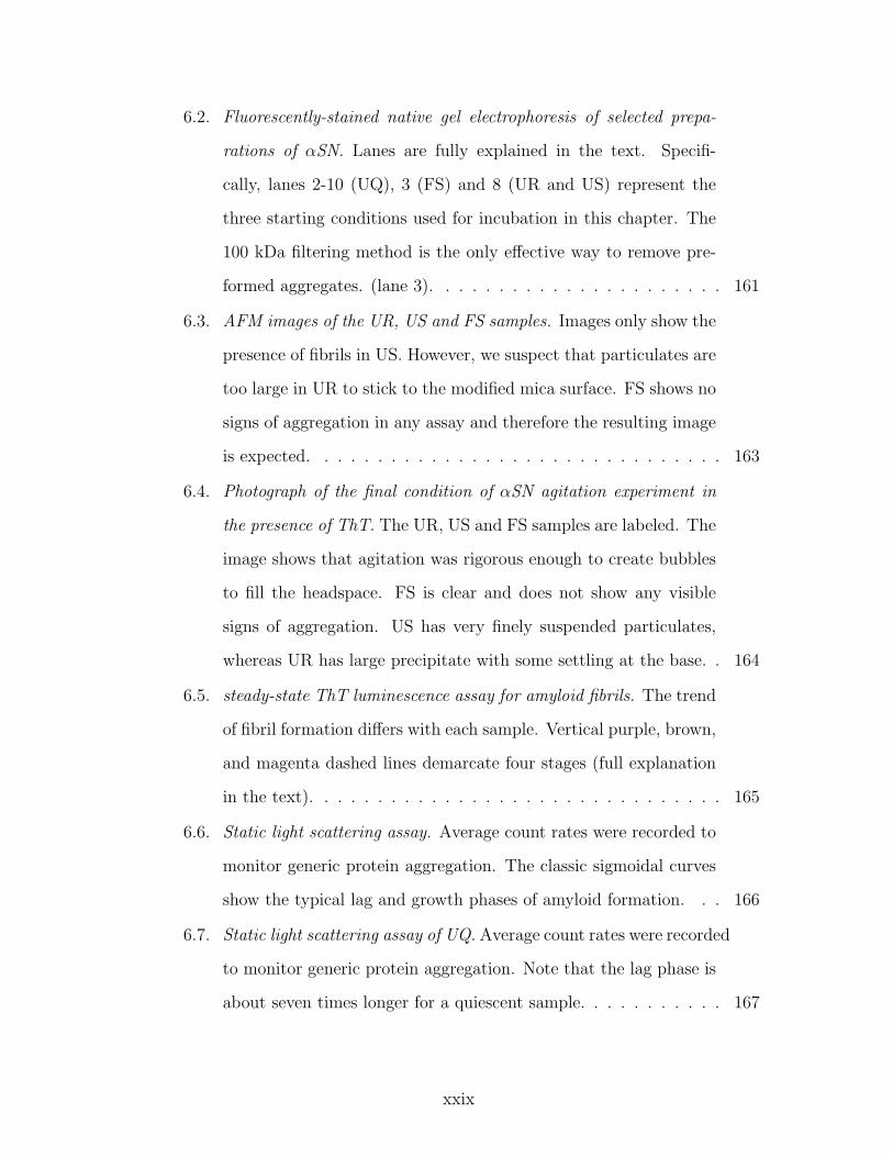
6.2. Fluorescently-stained native gel electrophoresis of selected prepa-
rations of αSN. Lanes are fully explained in the text. Specifi-
cally, lanes 2-10 (UQ), 3 (FS) and 8 (UR and US) represent the
three starting conditions used for incubation in this chapter. The
100 kDa filtering method is the only effective way to remove pre-
formed aggregates. (lane 3). . . . . . . . . . . . . . . . . . . . . . 161
6.3. AFM images of the UR, US and FS samples. Images only show the
presence of fibrils in US. However, we suspect that particulates are
too large in UR to stick to the modified mica surface. FS shows no
signs of aggregation in any assay and therefore the resulting image
is expected. . . . . . . . . . . . . . . . . . . . . . . . . . . . . . . 163
6.4. Photograph of the final condition of αSN agitation experiment in
the presence of ThT. The UR, US and FS samples are labeled. The
image shows that agitation was rigorous enough to create bubbles
to fill the headspace. FS is clear and does not show any visible
signs of aggregation. US has very finely suspended particulates,
whereas UR has large precipitate with some settling at the base. . 164
6.5. steady-state ThT luminescence assay for amyloid fibrils. The trend
of fibril formation differs with each sample. Vertical purple, brown,
and magenta dashed lines demarcate four stages (full explanation
in the text). . . . . . . . . . . . . . . . . . . . . . . . . . . . . . . 165
6.6. Static light scattering assay. Average count rates were recorded to
monitor generic protein aggregation. The classic sigmoidal curves
show the typical lag and growth phases of amyloid formation. . . 166
6.7. Static light scattering assay of UQ. Average count rates were recorded
to monitor generic protein aggregation. Note that the lag phase is
about seven times longer for a quiescent sample. . . . . . . . . . . 167
xxix
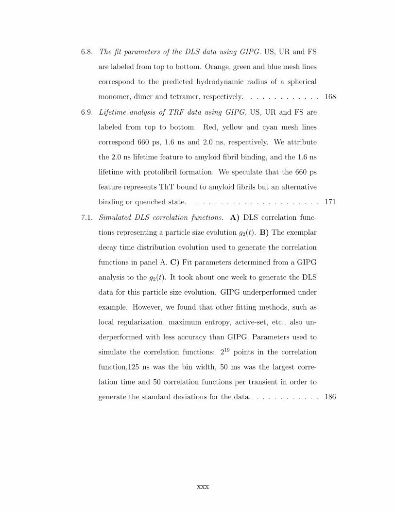
6.8. The fit parameters of the DLS data using GIPG. US, UR and FS
are labeled from top to bottom. Orange, green and blue mesh lines
correspond to the predicted hydrodynamic radius of a spherical
monomer, dimer and tetramer, respectively. . . . . . . . . . . . . 168
6.9. Lifetime analysis of TRF data using GIPG. US, UR and FS are
labeled from top to bottom. Red, yellow and cyan mesh lines
correspond 660 ps, 1.6 ns and 2.0 ns, respectively. We attribute
the 2.0 ns lifetime feature to amyloid fibril binding, and the 1.6 ns
lifetime with protofibril formation. We speculate that the 660 ps
feature represents ThT bound to amyloid fibrils but an alternative
binding or quenched state. . . . . . . . . . . . . . . . . . . . . . 171
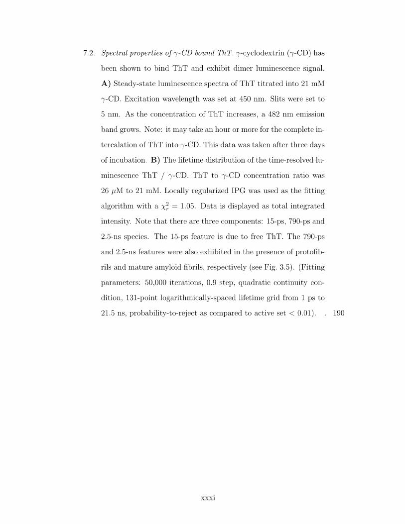
7.1. Simulated DLS correlation functions. A) DLS correlation func-
tions representing a particle size evolution g2(t). B) The exemplar
decay time distribution evolution used to generate the correlation
functions in panel A. C) Fit parameters determined from a GIPG
analysis to the g2(t). It took about one week to generate the DLS
data for this particle size evolution. GIPG underperformed under
example. However, we found that other fitting methods, such as
local regularization, maximum entropy, active-set, etc., also un-
derperformed with less accuracy than GIPG. Parameters used to
simulate the correlation functions: 219 points in the correlation
function,125 ns was the bin width, 50 ms was the largest corre-
lation time and 50 correlation functions per transient in order to
generate the standard deviations for the data. . . . . . . . . . . . 186
xxx
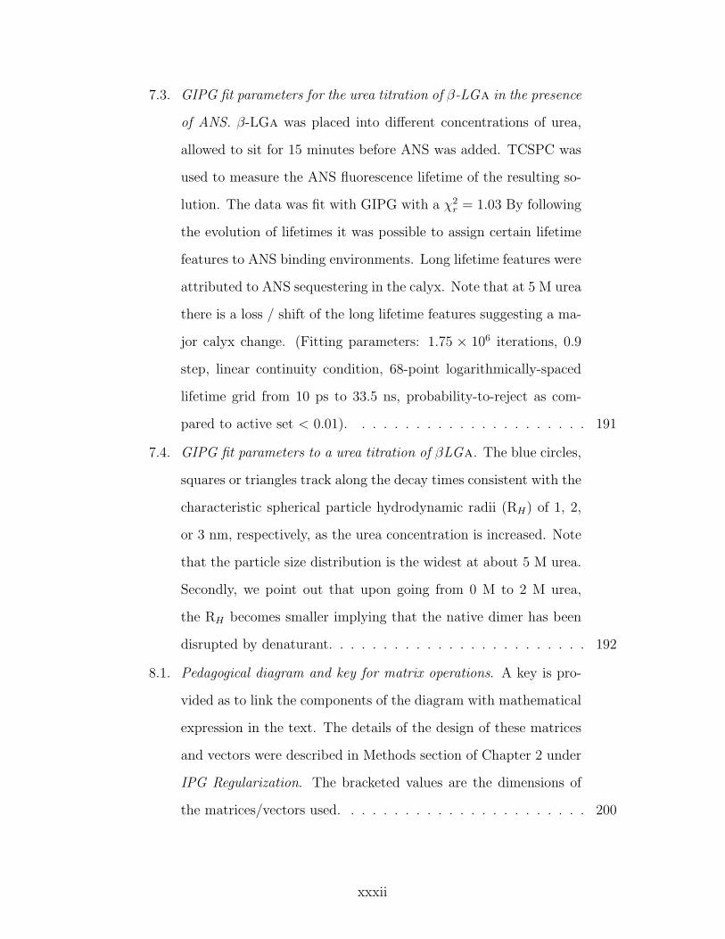
7.2. Spectral properties of γ-CD bound ThT. γ-cyclodextrin (γ-CD) has
been shown to bind ThT and exhibit dimer luminescence signal.
A) Steady-state luminescence spectra of ThT titrated into 21 mM
γ-CD. Excitation wavelength was set at 450 nm. Slits were set to
5 nm. As the concentration of ThT increases, a 482 nm emission
band grows. Note: it may take an hour or more for the complete in-
tercalation of ThT into γ-CD. This data was taken after three days
of incubation. B) The lifetime distribution of the time-resolved lu-
minescence ThT / γ-CD. ThT to γ-CD concentration ratio was
26 µM to 21 mM. Locally regularized IPG was used as the fitting
algorithm with a χ2r = 1.05. Data is displayed as total integrated
intensity. Note that there are three components: 15-ps, 790-ps and
2.5-ns species. The 15-ps feature is due to free ThT. The 790-ps
and 2.5-ns features were also exhibited in the presence of protofib-
rils and mature amyloid fibrils, respectively (see Fig. 3.5). (Fitting
parameters: 50,000 iterations, 0.9 step, quadratic continuity con-
dition, 131-point logarithmically-spaced lifetime grid from 1 ps to
21.5 ns, probability-to-reject as compared to active set < 0.01). . 190
xxxi
7.3. GIPG fit parameters for the urea titration of β-LGa in the presence
of ANS. β-LGa was placed into different concentrations of urea,
allowed to sit for 15 minutes before ANS was added. TCSPC was
used to measure the ANS fluorescence lifetime of the resulting so-
lution. The data was fit with GIPG with a χ2r = 1.03 By following
the evolution of lifetimes it was possible to assign certain lifetime
features to ANS binding environments. Long lifetime features were
attributed to ANS sequestering in the calyx. Note that at 5 M urea
there is a loss / shift of the long lifetime features suggesting a ma-
jor calyx change. (Fitting parameters: 1.75 × 10⁶ iterations, 0.9
step, linear continuity condition, 68-point logarithmically-spaced
lifetime grid from 10 ps to 33.5 ns, probability-to-reject as com-
pared to active set < 0.01). . . . . . . . . . . . . . . . . . . . . . 191
7.4. GIPG fit parameters to a urea titration of βLGa. The blue circles,
squares or triangles track along the decay times consistent with the
characteristic spherical particle hydrodynamic radii (RH) of 1, 2,
or 3 nm, respectively, as the urea concentration is increased. Note
that the particle size distribution is the widest at about 5 M urea.
Secondly, we point out that upon going from 0 M to 2 M urea,
the RH becomes smaller implying that the native dimer has been
disrupted by denaturant. . . . . . . . . . . . . . . . . . . . . . . . 192
8.1. Pedagogical diagram and key for matrix operations. A key is pro-
vided as to link the components of the diagram with mathematical
expression in the text. The details of the design of these matrices
and vectors were described in Methods section of Chapter 2 under
IPG Regularization. The bracketed values are the dimensions of
the matrices/vectors used. . . . . . . . . . . . . . . . . . . . . . . 200
xxxii
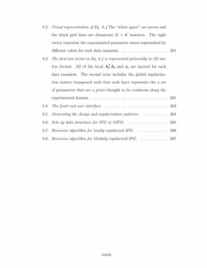
8.2. Visual representation of Eq. 8.4 The “white space” are zeroes and
the black grid lines are demarcate K × K matrices. The right
vector represent the concatenated parameter waves represented by
different colors for each data transient. . . . . . . . . . . . . . . . 201
8.3. The first two terms in Eq. 8.4 is represented pictorially in 3D ma-
trix format. All of the local ATl Al and xl are layered for each
data transient. The second term includes the global regulariza-
tion matrix transposed such that each layer represents the a set
of parameters that are a priori thought to be continous along the
experimental domain. . . . . . . . . . . . . . . . . . . . . . . . . . 201
8.4. The front end user interface. . . . . . . . . . . . . . . . . . . . . 203
8.5. Generating the design and regularization matrices. . . . . . . . . 204
8.6. Sets up data structures for IPG or GIPG. . . . . . . . . . . . . . 205
8.7. Recursive algorithm for locally regularized IPG. . . . . . . . . . . 206
8.8. Recursive algorithm for Globally regularized IPG. . . . . . . . . . 207
xxxiii
1
Chapter 1
Introduction
Personal motivation
Truth be told, I was resoundingly disinterested in pursuing a research career
studying biological molecules after graduating from college. It was during my
employment at Hoffmann-La Roche that I became aware of the importance of
increasing the stability and shelf life for protein-based therapeutic agents. Aggre-
gation was usually the biggest culprit in reducing the long-term efficacy of a drug;
we worked closely with the formulators to curb this effect. Concurrently, protein
aggregation research was becoming a popular topic, specifically because a small
peptide was found to be the main constituent of proteinaceous plaques found in
Alzheimer’s disease. [1, 2] The topic became personal when my grandfather was
diagnosed with this devastating disease. Motivation to study the physics and
chemistry of biological molecules stemmed from these events.1 This dissertation
is presented as the product of this motivation.
Disease
In the mid-1800s, German physician Rudolph Virchow first coined the term “amy-
loid” after iodine staining an abnormally appearing cerebral corpora amylacea
tissue culture. In 1906, Alois Alzheimer autopsied the brain of a patient who ex-
hibited premature senile dementia, along with paranoia and agitation, and found
1I also had an interest in inorganic chemistry but was throughly thwarted by enlisting inone Solid State Chemistry course at Rutgers University as a non-matriculated student in thespring of 2000. Professor’s name withheld.
2
neurofibrillary tangles and amyloid plaques. [3] In 1912, a colleague of Alzheimer,
Friedrich Heinrich Lewy, discovered protein inclusion bodies in the brains of pa-
tients with paralysis agitans. [4] Later, it was discovered that the inclusion bodies
also contained fibrillar protein deposits. Since these discoveries, 20 protein aggre-
gation diseases, including Alzheimers disease (AD), Parkinsons disease (PD), type
II diabetes, and Creutzfeldt-Jakobs disease, have been observed. The diseases
have a common thread: soluble polypeptides or proteins aggregate into insoluble
amyloid fibrils containing the cross-β structural motif. The enormous medical
implication of these diseases has motivated research and numerous reviews dis-
cussing the structure and growth of amyloid fibrils. [3, 5, 6, 7, 8, 2, 9, 10, 11]
PD affects 500,000 people in the United States. This is the second most
prevalent of the late-onset neurodegenerative diseases. [12] Today the disease is
clinically diagnosed much like it was done prior to Virchow’s amyloid discovery.
James Parkinson wrote an extensive essay on “Shaking Palsy” in 1817 (reprinted
in Ref.[13]) describing a patient with involuntary muscle tremors and inability to
initiate movements. Pathologically, PD is characterized by the predominate loss
of dopaminergic neurons in the substantia nigra. Dopamine, which is crucial to
human movement, is manufactured in this part of the brain. Upon autopsy, it
has been shown that some neurons have fibrillar cytoplasmic inclusions, or Lewy
bodies. [12] It is not clear, however, if the the presence of Lewy bodies and fibril
formation is the cause or the consequence of the neuronal death.
Recent evidence has shifted some of the focus from macroscopic fibrillar de-
posits to prefibrillar amyloidogenic aggregates as the cause of symptoms[14, 5,
15, 9], leading many to propose development of vaccines targeting small amy-
loidogenic aggregates.[7, 16, 2] In the case of PD, it has been shown that neurons
containing Lewy bodies appear to have no quantifiable differences in viability.

3
Secondly, the amount of Lewy bodies found in postmortem brains of asymp-
tomatic patients is ten-fold greater than the prevalence of PD. Thirdly, early-
onset familial forms of PD lead to neurodegeneration without substantial Lewy
body accumulation. [12] One hypothesis suggests that inclusion bodies sequester
toxic mis-folded or aggregated protein species from the system, akin to a protein
vacuum cleaner-like mechanism. [14] Transgenic animal experiments showed that
overexpression of the principle protein found Lewy bodies was not concomitant
to neuronal loss. However, transgenic mice with non-fibrillar deposits in parts of
the brain did exhibit substantial neuronal deficiencies. [9]
Placing the responsibility of the disease on toxic oligomers makes the solution
to the aggregation problem hard to ascertain. Proposed aggregation mechanisms
are constructed around the in vitro studies that show a sigmoidal growth of amy-
loid fibrils. The kinetics of the mechanism have been named lag, growth and
elongation (as labeled in Fig. 6.1). This may lead us to the notion that the
mechanism of protein aggregation simple.
Incubation time (days)
Monomer loss
seeds
Incubation time (days)
Monomer loss
Lag phase
Growth phase Mature
phase
Fibril production
Elongation
Phase
Figure 1.1: Classic sigmoidal kinetics of amyloid fibrils in vitro. Left panel: Thecanonical explanation of amyloid growth has been proposed from histologicalstaining assays in vitro. The explanation involves three phases: lag, growth andelongation. Right panel: Adding pre-formed seeds eliminates the lag phase. [17]See Fig. 1.2 for a comprehensive description of the possible intermediates thathave been proposed.
To the contrary, monitoring amyloid formation is only a small part of the entire
4
Figure 1.2: Overview of amyloid assembly mechanisms. Amyloid) any fibril,plaque, seed, or aggregate that has the characteristic cross-β sheet structure.Amyloid fibril) long ribbons of amyloid approximately 10 nm in diameterand >100 nm in length. Most often observed in vitro. Amyloid protofib-ril/filament) a species of amyloid smaller in diameter (3-6 nm) and length(<100 nm) than typical for amyloid fibrils, thought to be a possible direct precur-sor to amyloid fibrils perhaps through lateral aggregation. Amyloid seed (ortemplate)) a species of a critical size or structure that rapidly elongates to formlarger amyloid species possibly by providing a proper scaffold for amyloid assem-bly. Amyloidogenic oligomer) A small aggregate of precursor that is smallerthan the critical seed size but still may have some of the structural characteris-tics of amyloid. Folded state) The native (functional) state of the precursor.Folding intermediate) A partially folded or misfolded structure of the precur-sor. These partially folded structures are potentially the same as or precursorsto amyloidogenic folds. Denatured state) The unfolded state of the precursor.Unstructured aggregate) Completely or partially denatured proteins tend toaggregate non-specifically without forming a particular structural motif.
mechanism, and the vagueness in the sigmoidal kinetics can allow for many dif-
ferent possible mechanistic intermediates. Fig. 1.2 is a comprehensive diagram of
proposed intermediate species and pathways along the amyloid formation mech-
anism. It is well accepted that critical intermediates exist along the amyloid
pathway, but have not been explicitly identified. This combination has led to
5
a wide range of plausible mechanisms that do not violate sigmoidal growth of
amyloid fibril. Our interest is to shift focus from amyloid fibrils to prefibrillar
amyloidogenic aggregates that are present in the lag phase. Only by elucidating
the intermediate species can an accurate mechanism be developed. Unfortunately,
intermediate species are expected to be in relatively very low concentration. We
set out to confront this obstacle by utilizing several biophysical techniques in-
cluding time-resolved fluorescence (TRF) spectroscopy, dynamic light scattering
(DLS), and atomic force microscopy (AFM).
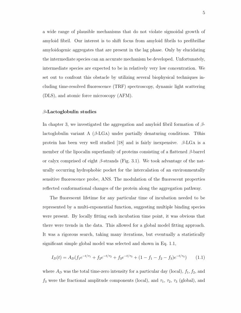
β-Lactoglobulin studies
In chapter 3, we investigated the aggregation and amyloid fibril formation of β-
lactoglobulin variant A (β-LGa) under partially denaturing conditions. T0his
protein has been very well studied [18] and is fairly inexpensive. β-LGa is a
member of the lipocalin superfamily of proteins consisting of a flattened β-barrel
or calyx comprised of eight β-strands (Fig. 3.1). We took advantage of the nat-
urally occurring hydrophobic pocket for the intercalation of an environmentally
sensitive fluorescence probe, ANS. The modulation of the fluorescent properties
reflected conformational changes of the protein along the aggregation pathway.
The fluorescent lifetime for any particular time of incubation needed to be
represented by a multi-exponential function, suggesting multiple binding species
were present. By locally fitting each incubation time point, it was obvious that
there were trends in the data. This allowed for a global model fitting approach.
It was a rigorous search, taking many iterations, but eventually a statistically
significant simple global model was selected and shown in Eq. 1.1,
ID(t) = AD(f1e−t/τ1 + f2e
−t/τ2 + f3e−t/τ3 + (1− f1 − f2 − f3)e−t/τ4) (1.1)
where AD was the total time-zero intensity for a particular day (local), f1, f2, and
f3 were the fractional amplitude components (local), and τ1, τ2, τ3 (global), and
6
τ4 (local) were the lifetimes.
Figure 1.3: Fit parameters of Eq. 1.1 used to described lifetime data of ANSbound BLG. This figure was originally part of my thesis proposal and is shown toillustrate the parameter trends after a global model was selected.
This analysis was presented as part of my research proposal as a requirement
for Ph.D. candidacy. The parameters from the global fit are shown in Fig. 1.3
and originally part of the proposal. The speculative mechanism was proposed
based on the data and is shown in Fig. 1.4. The mechanism was chosen based
on interpretation of the data which heavily relied on the global fit to reduce the
model space. Though we believed that the global model was supported by the
data, we understood that model selection is also related to the skill (and patience)
of the investigator selecting the model. This prompted us to think about ways
to develop (and not select) a model without unknowingly forbidding the true
solution.
7
Figure 1.4: Fit parameters of Eq. 1.1 used to described lifetime data of ANS boundBLG. This reduced data set originally appeared in my thesis proposal. τ1 and f1,and τ2 and f2 are attributed to sites 1 and 2, respectively. τ1 decreases withincreasing denaturant concentration, indicative of the disruption of the bindingpocket. At time-zero incubation, we assume that the protein is soluble but in anon-native state, S. During first six days, the site 1 lifetime decreases is indicativeof a further conformational change. S-state is converted to that of an aggregationprone state, A. The overall decrease in ANS binding to site 1 (f1) may be dueto a further conformational change as A-state monomers aggregate to O-stateoligomers that lack the internal binding pocket. It is also conceivable that theinablitiy for ANS to bind site 1 is a function of steric hindrance due to A-stateaggregation and not a conformational change in the binding pocket. The site2 binding occurs via external hydrophobic interactions. It is expected that anyhydrophobic exterior patches will be utilized by protein-protein interactions ofamyloid aggregation but may be affected by general oligomerization. By day 12,ANS external binding to site 2 becomes in competition with the specific protein-protein interactions necessary for amyloid cross-β structure, AM.
8
Using global probabilistic constraints to develop global models
Spectroscopic techniques often involve making a measurement on a system, mak-
ing a small perturbation to the system by some experimental factor, and then
taking another measurement. When done in this way, a smooth change in the
signal is expected. In chapter 2, we take advantage of this prior knowledge to cir-
cumvent the need to reduce model space in a single step. Instead, we develop an
approach that allows one to start from an essentially model-free fit and progress to
a specific model by moving from probabilistic constraints (parameter continuity
across the experimental coordinate) to deterministic constraints (global models).
In chapter 2, the globally regularized interior-point gradient method (GIPG)
is developed.2 We demonstrate through a pedagogical example, that GIPG could
represent a complex distribution of species on par with those thought to be present
during protein aggregation. Furthermore, we show how a maximum entropy
method approach may claim to be “model-free”, but does not significantly help
model development.
β-LGa revisited, model solidified
Chapter 3 is the recapitulation of the β-LGa data sets using GIPG analysis to
generate global models. By utilizing GIPG, lifetime evolution distributions were
calculated. We assumed that the contributions of different ANS-bound species
could be expressed as a linear combination of multipeaked “fingerprints”. This
type of fingerprint analysis, to our knowledge, is the first of its kind to be applied
to TCSPC data.
Time-resolved thioflavinT (ThT) luminescence was also analyzed by GIPG.
DLS data was fit with GIPG by adding a continuity condition to the particle size
2Chapter 7 is the explanation of the final version of the algorithm. Previous versions werecomputationally inefficient, but fully functional. By utilizing three dimensional matrix opera-tions, a drastic increase in the computational speed was reached.
9
distribution evolution. Though specific global models were not independently
developed for ThT and DLS data, the trends were considered when generating
fingerprints for the ANS fluorescence lifetimes.
The comprehensive interpretation of all the data led to an aggregation model
(Fig. 3.11) and kinetic scheme (Fig. 3.9). We cannot help but notice that the
original interpretation of the data did not change much with the inclusion of GIPG
analysis and DLS, AFM and ThT lifetime measurements. However, a deeper
understanding of the mechanism became available and allowed us to compare our
data to other mechanistic possibilities and alternative models.
Spectroscopic studies of covalently labeled αSyn
After comprehensive studies of β-LGa, it was now possible to begin studying
α-synuclein (αSyn) with confidence. αSyn is the principle component of Lewy
bodies, the protein inclusions bodies that are implicated in Parkinson’s disease.
One of the similarities carried over from the β-LGa studies is the conforma-
tional variability of the monomeric unit. (Recall that β-LGa formed amyloid
under partially denaturing conditions.) αSyn is an intrinsically disordered pro-
tein (IDP) but upon aggregation, goes through an ordered transition leading to
highly ordered cross-β quaternary structure. Amyloid-β peptide (in AD), Amylin
(in type II Diabetes) and prion protein (Creutzfeldt-Jakobs) are all intrinsically
disordered. [9].
Recent studies have shown that αSyn may have minimal structural prefer-
ences. [19, 20]. In these studies, long-range interactions were seen between the
negatively-charged C-terminal region with the middle region that is referred to as
the non-Aβ amyloid component, or NAC, region of αSyn. A recent NMR study
by our collaborator Baum et al., has pointed out that deprotecting the NAC re-
gion may lead to transient interchain interactions and may serve as a nucleation
site for aggregation. [21]
10
In chapter 3, we show how the intercalation of a conformationally sensitive
fluorophore can report on the aggregation states of a protein. β-LGa was a special
case where the host protein has a defined binding pocket. αSyn, on the other
hand, is an IDP. It is reasonable to expect that a non-covalent probe would non-
specifically bind. Therefore, covalent attachment of the fluorophore is necessary.
In chapter 4, temperature dependence of the fluorescence lifetimes of Alexa
Fluor, Atto 590, and Nile Red covalently attached to A19C mutant of αSyn are
evaluated. Previously, we have proven that we can analyze complicated fluores-
cence lifetime distributions with a model-free fitting approach. This approach
coupled with the notion that fluorescence is a highly sensitive technique, allows
us the unique opportunity to evaluate if, indeed, the fluorescence lifetime can
relay valuable information concerning the conformational dynamics of αSyn.
In chapter 5, a more traditional biophysical approach is taken to evaluate
conformational changes of αSyn. Specifically, CD and UV absorption are used to
monitor the spectroscopic changes αSyn with temperature. The two techniques
measure different features of protein. We notice transitions at different tem-
peratures for both techniques. These transitions are evaluated with a two-state
model. We invoke a “cooperativity” parameter to be incorporated into the parti-
tion function to create a fit function for the data. Cooperativity should be large
for folded to unfolded transitions, but for an IDP it is expected to be very close
to 1. Spectroscopically, however, the parameter was greater than 1, consistent
with the notion that αSyn has local transient conformations. [21]
Aggregation studies of αSyn
While researching the literature for aggregation rates of αSyn, we came across
awesome inconsistencies (see Table 6.2). Specifically, aggregation rates were the
most affected by preparation and incubation conditions. In chapter 6, we con-
duct a primary investigation of these conditions. We use the tools developed in

11
chapters 2 and 3, to evaluate the features in the particle size and ThT lifetimes
distributions and relate them to possible aggregation states of αSyn. We also
find that certain species along the amyloid pathway are not as pronounced under
certain preparation and incubation conditions.
The primary studies of the aggregation mechanism of αSyn is the conclusion
of this thesis work. However, it is just the beginning of an exciting set of ex-
periments designed to elucidate the amyloid formation mechanism of a medically
relevant protein. First, the proper analysis tools had to be developed (chapter 2)
and tested on a model system (chapter 3). With confidence in these tools, the
elucidating monomeric properties of αSyn using fluorescence techniques (chapters
4 and 5) could begin.
12
References
[1] Dennis J. Selkoe. Normal and abnormal biology of the β-amyloid precursorprotein. Annu. Rev. Neurosci., 17:489–517, 1994.
[2] John Hardy and Dennis J. Selkoe. The amyloid hypothesis of alzheimer’sdisease: progress and problems on the road to therapeutics. Science (Wash-ington, DC, U. S.), 297(5580):353–356, 2002.
[3] Jean D. Sipe and Alan S. Cohen. Review: History of the amyloid fibril.Journal of Structural Biology, 130(2/3):88–98, 2000.
[4] Bernd Holdorff. Friedrich heinrich lewy (1885-1950) and his work. J HistNeurosci., 11:19–28, 2002.
[5] Dominic M. Walsh, Dean M. Hartley, and Dennis J. Selkoe. The many facesof aβ: Structures and activity. Current Medicinal Chemistry: Immunology,Endocrine & Metabolic Agents, 3(4):277–291, 2003.
[6] Ronald Wetzel. Ideas of order for amyloid fibril structure. Structure (Cam-bridge, MA, U. S.), 10(8):1031–1036, 2002.
[7] Beka Solomon. Towards alzheimer’s disease vaccination. Mini-Rev. Med.Chem., 2(1):85–92, 2002.
[8] Marina D. Kirkitadze, Gal Bitan, and David B. Teplow. Paradigm shifts inalzheimer’s disease and other neurodegenerative disorders: the emerging roleof oligomeric assemblies. J. Neurosci. Res., 69(5):567–577, 2002.
[9] F. Chiti and C.M. Dobson. Protein misfolding, functional amyloid, andhuman disease. Annual Reviews Biochemistry, 75:333–366, 2006.
[10] David B. Teplow. Structural and kinetic features of amyloid β-protein fib-rillogenesis. Amyloid, 5(2):121–142, 1998.
[11] Jean-Christophe Rochet and Jr. Lansbury, Peter T. Amyloid fibrillogenesis:themes and variations. Curr. Opin. Struct. Biol., 10(1):60–68, 2000.
[12] Byron Caughey and Peter T. Lansbury Jr. Protofibrils, pores, fibrils, andneurodegeneration: Separating the responsible protein aggregates from theinnocent bystanders. Annu. Rev. Neurosci., 26:267–298, 2003.
[13] James Parkinson. An essay on the shaking palsy. J Neuropsychiatry ClinNeurosci, 14:223–236, 2002.
13
[14] Matthew S. Goldberg and Peter T. Lansbury Jr. Is there a cause-and-effectrelationship between α-synuclein fibrillization and parkinson’s disease? Na-ture Cell Biology, 2:E115–E119, 2000.
[15] Rakez Kayed, Elizabeth Head, Jennifer L. Thompson, Theresa M. McIn-tire, Saskia C. Milton, Carl W. Cotman, and Charles G. Glabe. Commonstructure of soluble amyloid oligomers implies common mechanism of patho-genesis. Science, 300:486–489, 2003.
[16] Dale Schenk. Opinion: Amyloid-β immunotherapy for alzheimer’s disease:the end of the beginning. Nat. Rev. Neurosci., 3(10):824–828, 2002.
[17] Eva Zerovnik. Amyloid-fibril formation. proposed mechanisms and relevanceto conformational disease. European Journal of Biochemistry, 269(14):3362–3371, 2002.
[18] Lindsay Sawyer and George Kontopidis. The core lipocalin, bovine β-lactoglobulin. Biochim. Biophys. Acta, 1482:136–148, 2000.
[19] Carlos W. Bertoncini, Young-Sang Jung, Claudio O. Fernandez, WolfgangHoyer, Christian Griesinger, Thomas M. Jovin, and Markus Zweckstetter.Release of long-range tertiary interactions potentiates aggregation of na-tively unstructured α-synuclein. Proc. Nat. Acad. Sci. U.S.A., 102:1430–1435, 2005.
[20] Matthew M. Dedmon, Kresten Lindorff-Larsen, John Christodoulou, MicheleVendruscolo, and Christopher M. Dobson. Mapping long-range interactionsin α-synuclein using spin-label nmr and ensemble molecular dynamics simu-lations. J. Am. Chem. Soc., 127:476–477, 2005.
[21] Kuen-Phon Wu, Seho Kim, David A. Fela, and Jean Baum. Characterizationof conformational and dynamic properties of natively unfolded human andmouse α-synuclein ensembles by nmr: Implication for aggregation. J. Mol.Bio., 378:1104–1115, 2008.
14
Chapter 2
Global fitting without a global model:
regularization based on the continuity of the
evolution of parameter distributions.
2.1 Summary
We introduce a new approach to global data fitting based on a regularization con-
dition that invokes continuity in the global data coordinate. Stabilization of the
data fitting procedure comes from probabilistic constraint of the global solution
to physically reasonable behavior rather than specific models of the system behav-
ior. This method is applicable to the fitting of many types of spectroscopic data
including dynamic light scattering (DLS), time-correlated single-photon counting
(TCSPC), and circular dichroism (CD). We compare our method to traditional
approaches to fitting an inverse Laplace transform by examining the evolution
of multiple lifetime components in synthetic TCSPC data. The global regular-
izer recovers features in the data that are not apparent from traditional fitting.
We show how our approach allows one to start from an essentially model-free fit
and progress to a specific model by moving from probabilistic to deterministic
constraints in both Laplace transformed and non-transformed coordinates.
15
2.2 Introduction
Sample heterogeneity is nearly unavoidable in spectroscopy. In many simple sys-
tems the heterogeneity can be reduced to the point where it can be ignored. How-
ever in complex biological systems there is much to be gained from understanding
the heterogeneity. The biological machinery in the cell, for example, relies on the
dynamic nature of proteins and protein assemblies.[1] Intermediate species have
been identified in protein (mis)folding mechanisms.[2, 3, 4, 5, 6] Multiple con-
formations of protein-ligand complexes have been discovered because of signal
heterogeneity.[7] The evolution of multiple binding sites for β-lactoglobulin and
the time-dependence of the site-binding entropy in response to the sudden pres-
ence of a strong dipole was elucidated by the heterogeneity in a time-dependent
Stokes-shift measurement.[8] Heterogeneity is a crucial element of interpreting sin-
gle molecule measurements.[9, 10, 11, 3, 12] The presence of multiple species in
misfolded β-lactoglobulin leads to very heterogeneous signals prior to[13, 14] and
during the assembly of amyloid.[15] To fully understand the underlying physics
of such complex systems requires approaches to data reduction that can accom-
modate their heterogeneity.
Data reduction, or fitting, always requires a model. For any phenomenon
being measured there is a set, or space, of models that could reasonably be ex-
pected to explain the data. The fitting procedure should eliminate all parts of
the model space inconsistent with the data. From the remaining possibilities, the
algorithm should allow selection of the most likely model given the experimental
information. Experimental information in this context includes both the explicit
data that comes from the instrumentation as well as knowledge that comes from
the experimental design and understanding of the physics of the system. These
two source of information we will call “data” and “prior knowledge.”[16]
Prior knowledge is used to determine the model space for the problem. Many
16
experiments — including quasi-elastic light scattering,[17, 18, 19, 20] circular
dichroism,[21] dynamic NMR,[22] and fluorescence lifetime[23] — can be related
to their underlying physics by Fredholm integral equations of the first kind:
F (t, y) =
∫ b
a
A(t, k, y) f(k, y) dk. (2.1)
Data inversion seeks to find the function, f(k, y), from the noisy signal, F (t, y) +
ε(t, y), given the continuous kernel function, A(t, k, y), that connects t and k, with
y remaining untransformed.
The mathematical model space comprises all possible functions f(k, y). In
most circumstances the physical interpretation of f(k, y) is that it represents a
distribution of populations of species that differ in their values of k. The goal
of the experiment is usually to determine the systematic behavior of those pop-
ulations with experimental changes in y, which can represent any experimental
condition such as pH, incubation time, solvent polarity, etc. For example, deter-
mining the species population changes with temperature allows thermodynamic
parameters to be extracted.
For experiments that monotonically decay such as fluorescence lifetime and dy-
namic light scattering measurements the kernel in Eq. 2.1 is A(t, k, y) = exp(−k t)
and a = 0, and b =∞ provide the integration limits for a Laplace transform:
F (t, y) = Lf(k, y) =
∫ ∞0
e−ktf(k, y) dk. (2.2)
Solving for f(k, y) requires inversion of integral equation 2.2.
In the presence of noise, the inverse Laplace transform is not unique. An
explicit expression for the inverse Laplace transform[24] illustrates the difficulty
of direct inversion,
f(k, y) = L−1F (t, y) = limi→∞
(−1)i
i!
[i
k
]i+1
F (i)
(i
k, x
)(2.3)
where F (i) is the ith derivative of F . The inverse Laplace transform is sensitive
to high order derivatives that do not exist in real data in any meaningful way;
17
each subsequent derivative increases the appearance of noise. As a result, all
functions, f(k, y), that have Laplace transforms, F (t, y), with similar first few
derivatives, but divergent higher order derivatives, will be valid solutions to the
inverse Laplace transform.
Since direct inversion is problematic, an indirect approach based on least-
squares optimization is typical.[25, 26, 27]
min
[(∫ b
a
A(t, k, y) f(k, y) dk − F (t, y)
)2]
(2.4)
Eq. 2.4, though more stable, still suffers from the problem that multiple solutions
for f(k, y) will be statistically equivalent. As a result, the strategy that a par-
ticular optimization algorithm uses to obtain the inversion, f(k, y), can influence
which solution is found, or even if a solution is found.
Many algorithms exist to solve the general least squares problem defined
by Eq. 2.4 and determine the inverse transform, f(k, y).[25, 26] A direct so-
lution to this problem can be obtained using methods such as singular value
decomposition.[26] However these approaches generate solutions that are highly
sensitive to the details of the noise and typically give many negative values for
the parameters. Therefore approaches that allow constraint of the solution to
positive values are desirable.
One of the most common methods for least-squares minimization is Levenberg-
Marquardt (LM).[28, 29] This method is fast for small to medium sized data
sets and is appropriate for both linear and non-linear models, but is subject to
potential non-linear instabilities.[26, 30] A gridded representation of the kernel
A(k, t, y) is called a design matrix and eliminates non-linear instabilities because
it allows the use of linear least squares algorithms like the Active-Set (AS) and the
Interior-Point Gradient (IPG) methods.[31, 32] Though the setup is common in
both methods, each minimizes the general least squares expression very differently.
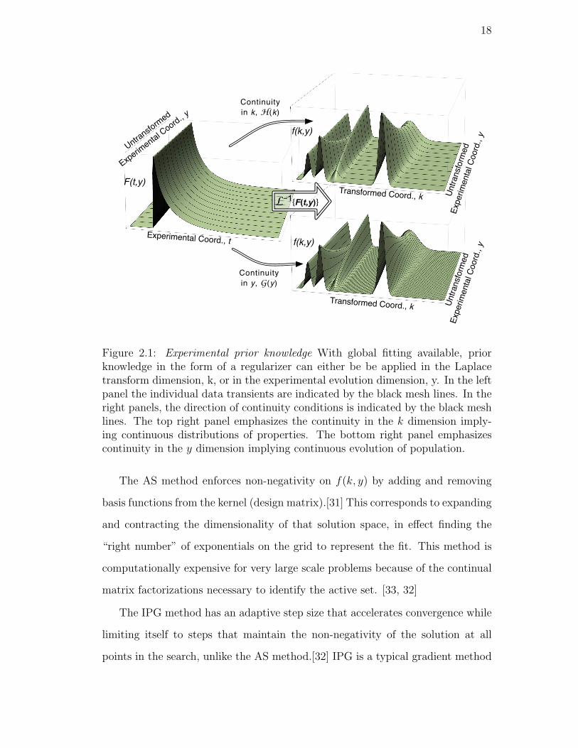
18
L-1F(t,y)
Transformed Coord., k
F(t,y)
f(k,y)
f(k,y)
Continuity
in k, H(k)
Continuity
in y, G(y)
Transformed Coord., k
Untransformed
Experimental Coord., y
Experimental Coord., t
Untransformed
Experimental Coord., y
Untransformed
Experimental Coord., y
Figure 2.1: Experimental prior knowledge With global fitting available, priorknowledge in the form of a regularizer can either be be applied in the Laplacetransform dimension, k, or in the experimental evolution dimension, y. In the leftpanel the individual data transients are indicated by the black mesh lines. In theright panels, the direction of continuity conditions is indicated by the black meshlines. The top right panel emphasizes the continuity in the k dimension imply-ing continuous distributions of properties. The bottom right panel emphasizescontinuity in the y dimension implying continuous evolution of population.
The AS method enforces non-negativity on f(k, y) by adding and removing
basis functions from the kernel (design matrix).[31] This corresponds to expanding
and contracting the dimensionality of that solution space, in effect finding the
“right number” of exponentials on the grid to represent the fit. This method is
computationally expensive for very large scale problems because of the continual
matrix factorizations necessary to identify the active set. [33, 32]
The IPG method has an adaptive step size that accelerates convergence while
limiting itself to steps that maintain the non-negativity of the solution at all
points in the search, unlike the AS method.[32] IPG is a typical gradient method

19
in that it uses the entire set of basis functions and requires only matrix-vector
multiplications.[34, 35] Though these methods are considered to be less accurate
than the traditional AS method [32], the decreased convergence time of IPG for
large problems makes it very useful. IPG accomplishes this by exploiting the
totally non-negative structure of the problem to calculate this step and direction
giving fits that converge faster than the classic Active-Set method.[32]
Because many different elements of the model space will give equally good fits
to the noisy data,[30] all three methods we mention must constrain the model
space, in some way, to stabilize the inverse Laplace transform. Since many of
the solutions may not be physically reasonable, constraints can be selected based
on prior knowledge. When f(k, y) is a population then f(k, y) ≥ 0. Instru-
mental limitations can limit the range of k that can be determined. When y is
varied systematically then the global behavior of the individual species popula-
tions can be invoked to limit the possible f(k, y). For example, the conservation
of matter could provide a normalization condition for f(k, y) at each value of
y. The systematic variation of y could provide an expectation of a particular
functional dependence of f(k, y) along y for particular values of k representing
different species. Limiting the model space with prior knowledge can be done
with deterministic or probabilistic constraints.
Constraints of both types may be applied to the transformed variable, k,
and the non-transformed variable, y. Constraints in the transformed variable
are formed from hypotheses regarding the nature of the system, f(k, y), across
k. This is illustrated by the upper right panel of Fig. 2.1 where continuity has
been invoked along k. Constraints in the non-transformed variable (such as time,
temperature, solvent, etc.) require hypotheses that generate global models leading
to specific functions or continuity conditions describing the evolution of the system
across y. This is illustrated by the lower right panel of Fig. 2.1.
Deterministic constraints consider only some very small subset of functions
20
in the model space, and forbid all non-conforming solutions. Such empirical
functions make the tacit prior assumption of a specific physical model for the
system that gives analytical forms for f(k, y) that transform trivially. A least-
squares fit to F (t, y) with these functions is equivalent to the inversion. The most
common way is to use a small number (i.e. 1-3) exponential functions to fit the
data. This limits the model space f(k, y) to a small number of delta functions. All
other possible solutions have their likelihood set to zero a priori. Global models
are constructed by assigning specific functions to describe the evolution of f(k, y)
along y for all of the discrete values of k that represent a species. A drawback
is that this can forbid the “true” solution from being obtained if it is not, by
happenstance, consistent with the deterministic constraints.
By contrast, probabilistic constraints reduce the likelihood of solutions in pro-
portion to their departure from the constraint, but do not set the likelihood of
any solutions in the model space to zero. Probabilistic constraints are usually
imposed by penalty functions or regularization conditions. The new fitting func-
tional including regularization is,
Ξ2 = χ2 + γΩ2, (2.5)
where χ2 is the usual sum of the weighted squared residuals, Ω2 is any arbitrary
regularizer functional, and γ is the strength of the regularization.
Early work on probabilistic constraints[30, 17] used a second derivative regu-
larizer functional of the form
Ω2 = H(k) =
∫ [∂2f(k, y)
∂k2
]2
dk (2.6)
with the assumption that this would provide the most “parsimonious” discretized
solution to the inversion problem.[17] This regularizer implies piece-wise linearity
in k, strongly biasing against any discontinuities. There will be many systems
for which this will not be valid, such as those having discrete distributions across
k. Other regularizers have been used to probabilistically reduce the available
21
solution space for the inversion by imposing expectations of the nature of the
solution in k.[36, 37]
Maximum entropy is another criterion that is often used as a regularizer [23,
36, 38, 39],
W =
∫ ∫f(k, y)−m(k, y)− f(k, y) log
(f(k, y)
m(k, y)
)dkdy (2.7)
where m(k, y) is the uniform distribution that gives maximum entropy. The
entropy functional satisfies two conditions that serve to define it. Entropy is
maximized for flat distributions. This has the physical meaning that all values of
k are not only possible but equally likely. Entropy also has the property that it
is maximized when, in a joint distribution, the likelihood is independent.[40, 16]
That is, when f(k, y) = f(k) × f(y). This has the physical meaning that all
species have identical behavior under the influence of the experimental variable.
This is an excellent example of how assumptions about the behavior of the system
can creep in without the explicit knowledge of the investigator. Also, since en-
tropy is an extensive property, performing a maximum entropy analysis globally
is identical to performing parallel local analyses, so long as the likelihood at each
value of y is normalized across k. This suggests that though maximum entropy
is a useful condition for probabilistic constraint of fitting, it is of limited benefit
for global fitting in this context.
In this paper we introduce a method to exploit the global behavior of a sys-
tem (e.g. continuity) across an experimental coordinate, y, to define a global
regularization condition that does not make any assumptions about the shape
or continuity in the Laplace transform dimension, k. In a typical experiment,
k is directly related some property of the different species present and the con-
centrations of the different species change with the experimental coordinate, y,
(e.g. over time by some kinetic rate law). Therefore the solution set, f(k, y), will
often be piece-wise continuous in y, implying smooth changes in the population of
individual species with respect to y. To represent this behavior mathematically,
22
we introduce a global regularizer that favors solutions that satisfy the continu-
ity/smoothness condition in y:
G(y) =
∫ [∂2f(k, y)
∂y2
]2
dy (2.8)
Implementation of Eq. 2.8 into Eq. 2.5 requires a general least-squares op-
timization algorithm that can accommodate the inclusion of a regularizer term.
The IPG method minimizes Eq. 2.4 by choosing the scale of the step and di-
rection to be as close as possible the exact minimizer without crossing into the
non-negative region. We augment the IPG with a regularizer functional such that
the step and direction favor solutions with continuity in the either the k, local,
or y, global, dimensions.
To demonstrate utility of global regularization on an evolving data set, we
simulate a test data set, evaluate fitting methods and compare and contrast ex-
isting method with methods introduced here. We also evaluate the effect of noise
on each method’s ability to reproduce the test parameter set. Lastly, we show
how to use global regularization in the experimental domain with a traditional
physical model for the species domain to do global fitting using LM.
2.3 Methods
2.3.1 IPG Regularizer
The computer implementation of Eq. 2.4 replaces continuous variables t, y, and
k with discrete variables ti, kj, and ylwith i ∈ 1 · · · T, j ∈ 1 · · ·K,
and l ∈ 1 · · ·Y . Matrix notation replaces continuous notation as follows. Each
transient, F (t, yl) has a design matrix,
A[T×K]l ≡ A(t, k, yl)/s(t, yl),
a solution vector,
x[K×1]l ≡ f(k, yl),
23
and a data vector,
b[T×1]l ≡ F (t, yl)/s(t, yl).
The design matrix and the data vector are scaled by the standard deviations of
the data, which were estimated by s(t, yl) =√F (t, yl) + 1.
We momentarily drop the subscripts in our notation when considering one
transient at a time. The minimum of Eq. 2.4 occurs when the derivatives with
respect to the parameters equal zero, yielding the exact minimizing equation,
ATAx−ATb = 0. (2.9)
The details of the fitting algorithm can be found in [32]. The key feature of the
algorithm is the way it determines the scaling vector for calculating each iteration:
d =x
ATAx. (2.10)
Eq. 2.10 is the core of the IPG algorithm and makes it less sensitive to ill-
conditioned problems. Ref. [32] shows that with condition number of ATA ≈
1016, the relative error of the fits between IPG and the Active-Set after 103 it-
erations is ≈ 10−5 and nearly five orders of magnitude better than other scaling
methods. For our global fits, typical condition numbers range from 1018 to 1022
making the insensitivity of IPG to condition number particularly valuable.
Locally Regularized IPG
The same minimization principle can be applied when considering the cost func-
tion, Ξ2 in (Eq. 2.5),
(ATA + γH)x−ATb = 0, (2.11)
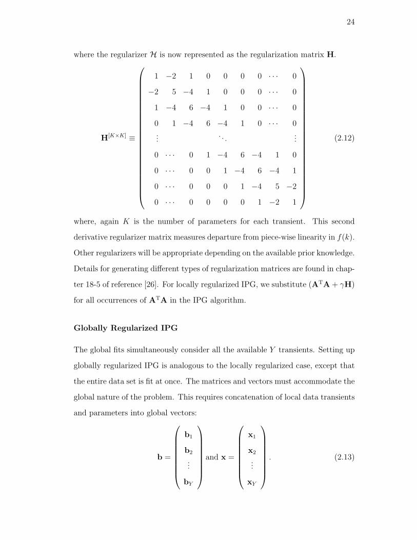
24
where the regularizer H is now represented as the regularization matrix H.
H[K×K] ≡
1 −2 1 0 0 0 0 · · · 0
−2 5 −4 1 0 0 0 · · · 0
1 −4 6 −4 1 0 0 · · · 0
0 1 −4 6 −4 1 0 · · · 0
.... . .
...
0 · · · 0 1 −4 6 −4 1 0
0 · · · 0 0 1 −4 6 −4 1
0 · · · 0 0 0 1 −4 5 −2
0 · · · 0 0 0 0 1 −2 1
(2.12)
where, again K is the number of parameters for each transient. This second
derivative regularizer matrix measures departure from piece-wise linearity in f(k).
Other regularizers will be appropriate depending on the available prior knowledge.
Details for generating different types of regularization matrices are found in chap-
ter 18-5 of reference [26]. For locally regularized IPG, we substitute (ATA + γH)
for all occurrences of ATA in the IPG algorithm.
Globally Regularized IPG
The global fits simultaneously consider all the available Y transients. Setting up
globally regularized IPG is analogous to the locally regularized case, except that
the entire data set is fit at once. The matrices and vectors must accommodate the
global nature of the problem. This requires concatenation of local data transients
and parameters into global vectors:
b =
b1
b2
...
bY
and x =
x1
x2
...
xY
. (2.13)
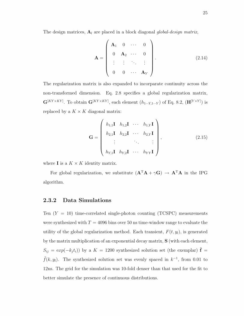
25
The design matrices, Al are placed in a block diagonal global-design matrix,
A =
A1 0 · · · 0
0 A2 · · · 0
......
. . ....
0 0 · · · AY
. (2.14)
The regularization matrix is also expanded to incorparate continuity across the
non-transformed dimension. Eq. 2.8 specifies a global regularization matrix,
G[KY×KY ]. To obtain G[KY×KY ], each element (h1···Y,1···Y ) of Eq. 8.2, (H[Y×Y ]) is
replaced by a K ×K diagonal matrix:
G =
h1,1I h1,2I · · · h1,Y I
h2,1I h2,2I · · · h2,Y I
.... . .
...
hY,1I hY,2I · · · hY Y I
, (2.15)
where I is a K ×K identity matrix.
For global regularization, we substitute (ATA + γG) → ATA in the IPG
algorithm.
2.3.2 Data Simulations
Ten (Y = 10) time-correlated single-photon counting (TCSPC) measurements
were synthesized with T = 4096 bins over 50 ns time-window range to evaluate the
utility of the global regularization method. Each transient, F (t, yl), is generated
by the matrix multiplication of an exponential decay matrix, S (with each element,
Sij = exp(−kjti)) by a K = 1200 synthesized solution set (the exemplar) f =
f(k, yl). The synthesized solution set was evenly spaced in k−1, from 0.01 to
12ns. The grid for the simulation was 10-fold denser than that used for the fit to
better simulate the presence of continuous distributions.
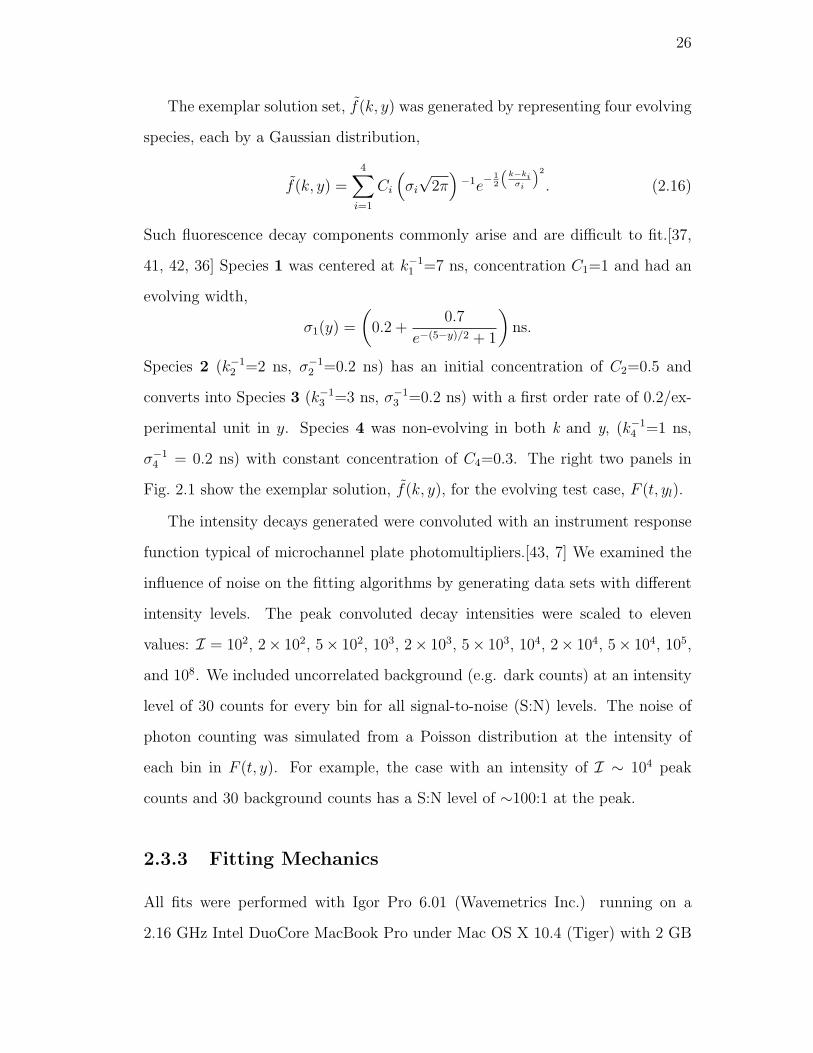
26
The exemplar solution set, f(k, y) was generated by representing four evolving
species, each by a Gaussian distribution,
f(k, y) =4∑i=1
Ci
(σi√
2π)−1e− 1
2
“k−kiσi
”2
. (2.16)
Such fluorescence decay components commonly arise and are difficult to fit.[37,
41, 42, 36] Species 1 was centered at k−11 =7 ns, concentration C1=1 and had an
evolving width,
σ1(y) =
(0.2 +
0.7
e−(5−y)/2 + 1
)ns.
Species 2 (k−12 =2 ns, σ−1
2 =0.2 ns) has an initial concentration of C2=0.5 and
converts into Species 3 (k−13 =3 ns, σ−1
3 =0.2 ns) with a first order rate of 0.2/ex-
perimental unit in y. Species 4 was non-evolving in both k and y, (k−14 =1 ns,
σ−14 = 0.2 ns) with constant concentration of C4=0.3. The right two panels in
Fig. 2.1 show the exemplar solution, f(k, y), for the evolving test case, F (t, yl).
The intensity decays generated were convoluted with an instrument response
function typical of microchannel plate photomultipliers.[43, 7] We examined the
influence of noise on the fitting algorithms by generating data sets with different
intensity levels. The peak convoluted decay intensities were scaled to eleven
values: I = 102, 2× 10², 5× 10², 103, 2× 10³, 5× 10³, 104, 2× 10⁴, 5× 10⁴, 105,
and 108. We included uncorrelated background (e.g. dark counts) at an intensity
level of 30 counts for every bin for all signal-to-noise (S:N) levels. The noise of
photon counting was simulated from a Poisson distribution at the intensity of
each bin in F (t, y). For example, the case with an intensity of I ∼ 104 peak
counts and 30 background counts has a S:N level of ∼100:1 at the peak.
2.3.3 Fitting Mechanics
All fits were performed with Igor Pro 6.01 (Wavemetrics Inc.) running on a
2.16 GHz Intel DuoCore MacBook Pro under Mac OS X 10.4 (Tiger) with 2 GB
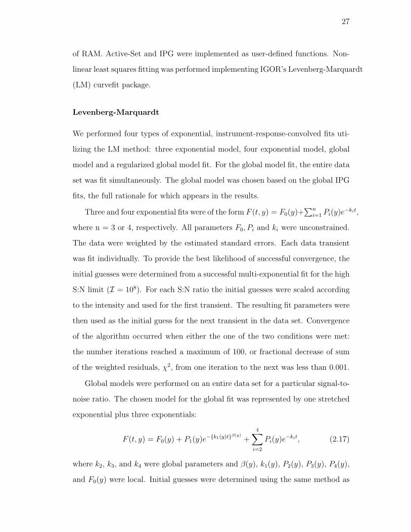
27
of RAM. Active-Set and IPG were implemented as user-defined functions. Non-
linear least squares fitting was performed implementing IGOR’s Levenberg-Marquardt
(LM) curvefit package.
Levenberg-Marquardt
We performed four types of exponential, instrument-response-convolved fits uti-
lizing the LM method: three exponential model, four exponential model, global
model and a regularized global model fit. For the global model fit, the entire data
set was fit simultaneously. The global model was chosen based on the global IPG
fits, the full rationale for which appears in the results.
Three and four exponential fits were of the form F (t, y) = F0(y)+∑n
i=1 Pi(y)e−kit,
where n = 3 or 4, respectively. All parameters F0, Pi and ki were unconstrained.
The data were weighted by the estimated standard errors. Each data transient
was fit individually. To provide the best likelihood of successful convergence, the
initial guesses were determined from a successful multi-exponential fit for the high
S:N limit (I = 108). For each S:N ratio the initial guesses were scaled according
to the intensity and used for the first transient. The resulting fit parameters were
then used as the initial guess for the next transient in the data set. Convergence
of the algorithm occurred when either the one of the two conditions were met:
the number iterations reached a maximum of 100, or fractional decrease of sum
of the weighted residuals, χ2, from one iteration to the next was less than 0.001.
Global models were performed on an entire data set for a particular signal-to-
noise ratio. The chosen model for the global fit was represented by one stretched
exponential plus three exponentials:
F (t, y) = F0(y) + P1(y)e−k1(y)tβ(y)
+4∑i=2
Pi(y)e−kit, (2.17)
where k2, k3, and k4 were global parameters and β(y), k1(y), P2(y), P3(y), P4(y),
and F0(y) were local. Initial guesses were determined using the same method as
28
the local fits. All parameters were constrained to be positive, and the following
parameters were constrained by 0.8 < k−14 < 1.2 ns, 1.5 < k−1
2 < 2.5 ns, 2.8 <
k−13 < 3.5 ns, and β ≤ 1. The rationale for the constraints is in the Results sec-
tion. A perturbation coefficient applied to stabilize the estimates of the numerical
derivatives calculated by LM and was necessary for a successful fit. In IGOR Pro,
the coefficient is implemented via an “epsilon wave” and was set to 0.01. The
convergence criteria were the same as the local LM fits.
The globally regularized model applies the second derivative global continuity
condition on same local parameters across the non-transformed coordinate. The
regularizer for any set of local parameters, P(Y×1), is:
Ω2P = PTHP (2.18)
where H ≡ H(Y×Y) and P ≡ (local1, local2, ...localY )T. A regularizer value for
any set of parameters can be calculated. For this paper, regularizer value for
local parameters P1(y), P2(y), P3(y), P4(y), k1(y) and β(y) were caluculated and
summed into the total regularizer value for the model, Ω2M.
In order to use the same LM minimizer used to fit the three and four expo-
nential fits, Igor’s built in curve fitting operation was used to minimize the new
cost function in Eq. 2.5. This was accomplished by expanding the data and fit by
one data point (a total of T × Y + 1 points). By placing the square root of γΩ2M
in the last fit point and a zero in the last data point, the fitting algorithm will
add the squared the difference to the residuals giving the proper cost function.
Active-Set and Interior Point Gradient
AS and IPG require as input a design matrix (Al), scaled data (bl), and an
initial guess for the solution xl. AS, IPG and locally regularized IPG fit each
transient in a data set individually. For TCSPC data simulations in this paper
the design matrix A has elements exp(−kjti). The design matrix was convoluted
29
column-by-column with an instrument response function typical of microchannel
plate photomultipliers. The total number of grid points per local fit was set to
K = 120. The grid was evenly spaced in k−1 from 0.1 to 12.0 ns. For globally
regularized IPG, these local matrices were organized as previously described in
the methods for the global case.
The IPG method requires a scaling term λ ∈ (0, 1) The scaling term is used
when IPG attempts to take step into a non-feasible region of the parameter state
space; λ is used to scale the maximum allowable step distance as to get close, but
not reach the non-negative boundary. We set λ = 0.9 which is 90% of the largest
step. In the current data fits λ was set to 0.9 because it seemed to converge the
fastest while also avoiding local minima.
Convergence of the IPG algorithm was allowed a maximum of 106 iterations.
Every 2000 iterations, χ2 was evaluated. If the fractional decrease from one
evaluation χ2 to the next was less than 10−7, the fit was considered converged.
The high S:N limit data, I = 108 required 107 iterations due to the large condition
number of the global design matrix. Initial guesses were set to 10−32.
We chose the linear continuity condition for both local regularization and for
global regularization in Eq. 2.6 and 2.8, respectively. Adding the regularizer to
the minimization for IPG modifies the condition needed to maintain the param-
eters in the non-negative region. To maintain the totally non-negative condition,
regularized IPG requires (ATA + γH)x > 0, so γ is constrained by:
γ ≤ Hx
ATAx. (2.19)
For all S:N, γ was set many orders of magnitude below this maximum threshold.
Maximum Entropy method fits
Maximum Entropy fits were performed using a exponential rates and is minimized
by the Levenberg-Marquardt method using the same convergence and constraint

30
criteria as described above. Each transient was fit locally using the the same
design matrices, Al, as employed for the AS and IPG methods,
F (t, yl) =T∑i=1
K∑j=1
Aijlxjl. (2.20)
Maximum Entropy regularizer, γW , was by calculated using Eq.2.7 and were
implemented using Igor’s built in curve fitting operation in similar fashion as the
global regularized model fits.
2.3.4 Model Similarity Criteria
Two perspectives can be taken to compare and contrast the fitting methods pre-
sented in this paper. The first compares the quality of fit, the second compares
the quality of parameters. A model is considered acceptable when the quality-of-
fit, χ2, is below some statistcal threshold . Multiple acceptable models (usually
differing in model simplicity) can be differentiated from each other via statisti-
cal testing. However, many models will be statistically indistinguishable based
solely on quality of fit to the data, even when χ2 is evaluated globally across
all Y transients, frustrating the search for the “best” global model. The ulti-
mate goal is to get the set of parameters that best represents the physics of the
system assuming all candidate models give adequate fits to the data. We use
the Kullback-Leibler divergence and species population deviation to evaluate the
quality of the parameters as compared to the exemplar parameter set.
Quality-of-fit
The sum of the weighted, squared residuals, χ2, is normally reduced by the ex-
pected variance or value of χ2 based on normal statistics. However, because we
have synthesized data, we can directly compare the true F(t,y) (i.e. noiseless
data) to the noisy data to determine the actual variance of the data and reduce
31
the fit χ2 by this value,
χ2r =
χ2fit
χ2true
. (2.21)
χ2r values are calculated for the entire data set. We consider an adequate fit to
be 1.1 > χ2r > 1.0. χ2
r with values above or below this range under-fitting or
over-fitting the data, respectively.
The F-test is used to calculate the probability-to-reject the hypothesis that two
fits are the same based on χ2r [17]. Values close to 1 indicate the values of χ2
r are
statistically different. For this paper, we use the F-test for two different purposes:
to set convergence criteria and to compare the statistical significance of different
model fits. The convergence criteria for IPG fits provided a probability-to-reject
< 0.01 for all S:N when compared to the AS fits. The regularizer strength, γ, for
local and globally regularized IPG fits was chosen such that probability-to-reject
< 0.01 when compared to the AS fits. With very little regularization, we will show
that even though fits are not statistically different, the underlying parameters
distributions are. The F-test was used compare traditional global model fitting
with regularized global fitting, again choosing the regularization strength such
that probability-to-reject < 0.01. We also used the F-test to compare three
exponential fit to the four exponential, traditional global fit and regularized global
fits.
Quality-of-Parameters
Kullback-Leibler divergence is an information theory approach to quantify the
difference between a “true” probability distribution and an arbitrary probability
distribution, and represented by,
DKL =∑k
∑y
f(k, y) ln
(f(k, y)
f(k, y)
). (2.22)
DKL is a measure of the relative entropy of the two distributions. Perfect overlap
of a test set would result in a value of DKL = 0.
32
A common goal in fitting data is to determine the evolution of the populations
of different species. Attribution of the populations from gridded fits such as the
AS and IPG methods described above is not trivial. Therefore, we define regions
of the grid that are attributed to each species. The region for each species is
summed for a given value of y to determine the total population of that species.
The evolution of species i in a particular data set was defined as Si(y):
Si(y) =
ki,max∑k=ki,min
f(k, y) (2.23)
where ki,min and ki,max were set based on the features of the exemplar parameter
set. Specifically, k−14,min = 0.6 ns, k−1
4,max = 1.4 ns, k−12,min = 1.5 ns, k−1
2,max = 2.4 ns,
k−13,min = 2.5 ns, k−1
3,max = 3.5 ns and k−11,min = 5.0 ns, k−1
1,max = 9.0 ns. The species
parameters are calculated for every S:N ratio, but we will only explicitly compare
Si’s for different fitting methods at I = 104.
An overall score for reproducing the populations over the evolution dimension
y was determined by the mean-squared difference of the populations:
POP =4∑i=1
(Si(y)− Si(y))2 (2.24)
where Si(y) is the population vectors calculated from the exemplar model. This
metric, along with the Kullback-Leibler divergence, alllowed us to score the overall
performance of different methods for all S:N ratios in their ability to reproduce
the underlying physics of the system.
2.3.5 Error Estimates
Parameter errors in ill-posed problems are unbounded.[17] This arises because
many potentially very different parameter sets can fit the data equally-well. How-
ever for a particular fit one can estimate the errors in the parameters and the
degree to which they are coupled from diagonal and off diagonal elements of the
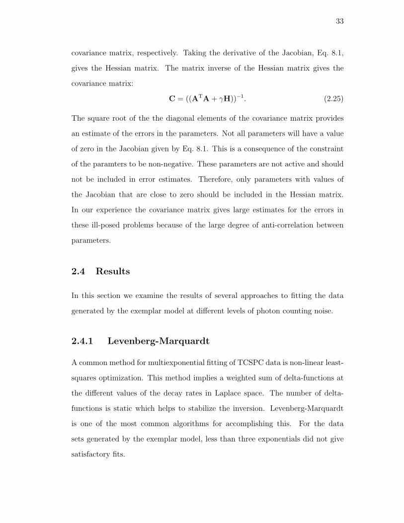
33
covariance matrix, respectively. Taking the derivative of the Jacobian, Eq. 8.1,
gives the Hessian matrix. The matrix inverse of the Hessian matrix gives the
covariance matrix:
C = ((ATA + γH))−1. (2.25)
The square root of the the diagonal elements of the covariance matrix provides
an estimate of the errors in the parameters. Not all parameters will have a value
of zero in the Jacobian given by Eq. 8.1. This is a consequence of the constraint
of the paramters to be non-negative. These parameters are not active and should
not be included in error estimates. Therefore, only parameters with values of
the Jacobian that are close to zero should be included in the Hessian matrix.
In our experience the covariance matrix gives large estimates for the errors in
these ill-posed problems because of the large degree of anti-correlation between
parameters.
2.4 Results
In this section we examine the results of several approaches to fitting the data
generated by the exemplar model at different levels of photon counting noise.
2.4.1 Levenberg-Marquardt
A common method for multiexponential fitting of TCSPC data is non-linear least-
squares optimization. This method implies a weighted sum of delta-functions at
the different values of the decay rates in Laplace space. The number of delta-
functions is static which helps to stabilize the inversion. Levenberg-Marquardt
is one of the most common algorithms for accomplishing this. For the data
sets generated by the exemplar model, less than three exponentials did not give
satisfactory fits.
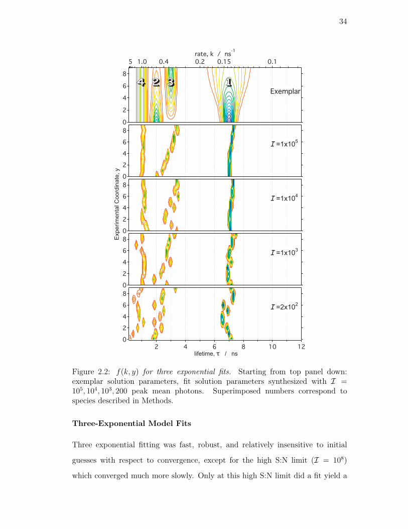
34
8
6
4
2
0
12108642 lifetime, t / ns
8
6
4
2
0
8
6
4
2
0
Exp
erim
en
tal C
oo
rdin
ate
, y
8
6
4
2
0
8
6
4
2
0
5 1.0 0.4 0.2 0.15 0.1
rate, k / ns-1
44 22 33 11Exemplar
I =1x10⁵
I =1x10⁴
I =1x10³
I =2x10²
Figure 2.2: f(k, y) for three exponential fits. Starting from top panel down:exemplar solution parameters, fit solution parameters synthesized with I =105, 104, 103, 200 peak mean photons. Superimposed numbers correspond tospecies described in Methods.
Three-Exponential Model Fits
Three exponential fitting was fast, robust, and relatively insensitive to initial
guesses with respect to convergence, except for the high S:N limit (I = 108)
which converged much more slowly. Only at this high S:N limit did a fit yield a

35
value of χ2r that indicated that the fit failed to reproduce the data. (See Fig. 2.11.)
Contour plots of the parameter values resulting from three exponential LM fits
appear in Fig. 2.2. The discrete functions are unable to reproduce the width or
evolution of Species 1 at any S:N. The conversion of Species 2 to Species 3 is never
resolved. At high S:N (I ≥ 105) the conversion is represented by a single species
with a decay rate at approximately the weighted average of the contributions of
Species 2 and 3. Species 4 should not evolve in either intensity or position and
is only properly reproduced at high S:N (I ≥ 105).
The population evolutions for Species 1 - 4 at a moderate S:N, I = 104, are
compiled in Fig. 2.14. For this three exponential fit, S1(y), represented by brown
circles, follows a similar trend to that of the exemplar evolution (shown by the
solid line of the same color). S2(y) (green diamonds) is not present, suggesting
the need for another exponential term. S3(y) (blue triangles) follows the cor-
rect increasing population evolution trend over the experiment coordinate, but is
overestimated. S4(y) (red squares) decreases until it reaches the true population,
y = 2, then flattens. The initial overestimation of Species 4 population evolution
and total overestimation of Species 3 is a compensation for the inadequacy of the
three exponential model to describe Species 2.
Quantitative measure of the similarity (see DKL and POP in Figs. 2.12 and
2.13, respectively) of the three exponential fit parameters and the exemplar model
show little improvement with increasing S:N, even at the high limit (I = 108).
This is a consequence of the lack of flexibility in the model to represent the trends
in the exemplar model. In effect, the correct model was excluded prior to fitting.
A normal next step would be to add an additional exponential term to the model
and compare the fits to the three exponential results.
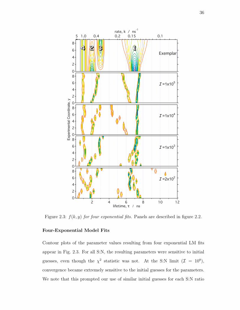
36
8
6
4
2
0
12108642lifetime, t / ns
8
6
4
2
0
8
6
4
2
0
Experim
enta
l C
oord
inate
, y
8
6
4
2
0
8
6
4
2
0
5 1.0 0.4 0.2 0.15 0.1
rate, k / ns-1
44 22 33 11Exemplar
I =1x10⁵
I =1x10⁴
I =1x10³
I =2x10²
Figure 2.3: f(k, y) for four exponential fits. Panels are described in figure 2.2.
Four-Exponential Model Fits
Contour plots of the parameter values resulting from four exponential LM fits
appear in Fig. 2.3. For all S:N, the resulting parameters were sensitive to initial
guesses, even though the χ2 statistic was not. At the S:N limit (I = 108),
convergence became extremely sensitive to the initial guesses for the parameters.
We note that this prompted our use of similar initial guesses for each S:N ratio
37
as described in the Methods. According to the F-test, the χ2r values were not
significantly different from those obtained for three exponential fits until high
S:N (probability-to-reject for I ≤ 2 × 10⁴ was < 0.01). Only the high S:N limit
(I = 108) gave a value of χ2r that indicated that the fit failed to reproduce the
data. (See Fig. 2.11).
The four-exponential model fails to reproduce the exemplar model as illus-
trated in Fig.2.3. In the region of the distribution associated with Species 1, the
fit typically used two of the four available exponentials. There was no systematic
trend in these components until high S:N (I ≥ 105) where the pair of exponen-
tials are split and increases in separation over the non-transformed coordinate,
y. Though this might have been hailed as a success, there is little to distinguish
this pattern from that generated in the Species 2, 3, and 4 region. Here Species
4 is resolved, and the exchange of Species 2 and 3 is again reduced to a single
exponential at the weighted mean.
These trends can be more clearly seen when we consider the species population
evolutions in Fig. 2.14. The S1(y) decreases and diverges from the exemplar at
y = 6 as the one of the two exponential rates, attempting to shape the edges of this
distribution, overshifted to about k−1 = 4.5 ns. There was an abrupt exchange of
population between S2(y) and S3(y) at y = 6 as the single exponential component
shifts to longer lifetime. Finally, S4(y) evolved by first decreasing (y ≤ 5) then,
after a sharp increase, decreased again (y > 6).
The overall population overlap parameter, POP , was overall better than the
three exponential fits and gradually, if inconsistently, trended toward improve-
ment with increasing S:N. The Kullback-Liebler divergence also improved slightly
with increasing S:N. Approaching the high S:N limit there was no further improve-
ment in POP or in DKL. Interestingly, χ2r greatly deviated from one but was two
orders of magnitude smaller than three exponential χ2r at the same high S:N limit.
At low S:N the fits are of such poor stability that the addition of another
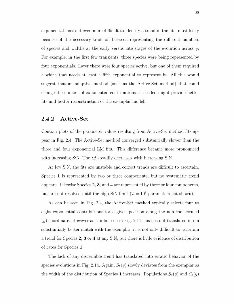
38
exponential makes it even more difficult to identify a trend in the fits, most likely
because of the necessary trade-off between representing the different numbers
of species and widths at the early versus late stages of the evolution across y.
For example, in the first few transients, three species were being represented by
four exponentials. Later there were four species active, but one of them required
a width that needs at least a fifth exponential to represent it. All this would
suggest that an adaptive method (such as the Active-Set method) that could
change the number of exponential contributions as needed might provide better
fits and better reconstruction of the exemplar model.
2.4.2 Active-Set
Contour plots of the parameter values resulting from Active-Set method fits ap-
pear in Fig. 2.4. The Active-Set method converged substantially slower than the
three and four exponential LM fits. This difference became more pronounced
with increasing S:N. The χ2r steadily decreases with increasing S:N.
At low S:N, the fits are unstable and correct trends are difficult to ascertain.
Species 1 is represented by two or three components, but no systematic trend
appears. Likewise Species 2, 3, and 4 are represented by three or four components,
but are not resolved until the high S:N limit (I = 108 parameters not shown).
As can be seen in Fig. 2.4, the Active-Set method typically selects four to
eight exponential contributions for a given position along the non-transformed
(y) coordinate. However as can be seen in Fig. 2.11 this has not translated into a
substantially better match with the exemplar; it is not only difficult to ascertain
a trend for Species 2, 3 or 4 at any S:N, but there is little evidence of distribution
of rates for Species 1.
The lack of any discernible trend has translated into erratic behavior of the
species evolutions in Fig. 2.14. Again, S1(y) slowly deviates from the exemplar as
the width of the distribution of Species 1 increases. Populations S2(y) and S3(y)
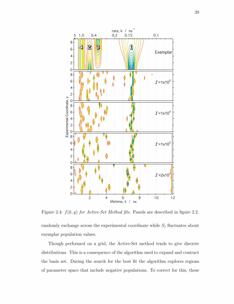
39
8
6
4
2
0
12108642lifetime, t / ns
8
6
4
2
0
8
6
4
2
0
Exp
erim
en
tal C
oo
rdin
ate
, y
8
6
4
2
0
8
6
4
2
0
5 1.0 0.4 0.2 0.15 0.1
rate, k / ns-1
44 22 33 11Exemplar
I =1x10⁵
I =1x10⁴
I =1x10³
I =2x10²
Figure 2.4: f(k, y) for Active-Set Method fits. Panels are described in figure 2.2.
randomly exchange across the experimental coordinate while S1 fluctuates about
exemplar population values.
Though performed on a grid, the Active-Set method tends to give discrete
distributions. This is a consequence of the algorithm used to expand and contract
the basis set. During the search for the best fit the algorithm explores regions
of parameter space that include negative populations. To correct for this, these
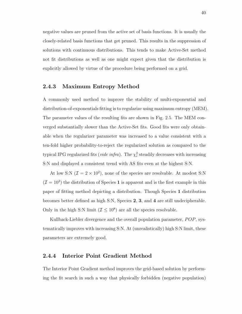
40
negative values are pruned from the active set of basis functions. It is usually the
closely-related basis functions that get pruned. This results in the suppression of
solutions with continuous distributions. This tends to make Active-Set method
not fit distributions as well as one might expect given that the distribution is
explicitly allowed by virtue of the procedure being performed on a grid.
2.4.3 Maximum Entropy Method
A commonly used method to improve the stability of multi-exponential and
distribution-of-exponentials fitting is to regularize using maximum entropy (MEM).
The parameter values of the resulting fits are shown in Fig. 2.5. The MEM con-
verged substantially slower than the Active-Set fits. Good fits were only obtain-
able when the regularizer parameter was increased to a value consistent with a
ten-fold higher probability-to-reject the regularized solution as compared to the
typical IPG regularized fits (vide infra). The χ2r steadily decreases with increasing
S:N and displayed a consistent trend with AS fits even at the highest S:N.
At low S:N (I = 2× 10²), none of the species are resolvable. At modest S:N
(I = 103) the distribution of Species 1 is apparent and is the first example in this
paper of fitting method depicting a distribution. Though Species 1 distribution
becomes better defined as high S:N, Species 2, 3, and 4 are still undecipherable.
Only in the high S:N limit (I ≤ 108) are all the species resolvable.
Kullback-Liebler divergence and the overall population parameter, POP , sys-
tematically improves with increasing S:N. At (unrealistically) high S:N limit, these
parameters are extremely good.
2.4.4 Interior Point Gradient Method
The Interior Point Gradient method improves the grid-based solution by perform-
ing the fit search in such a way that physically forbidden (negative population)
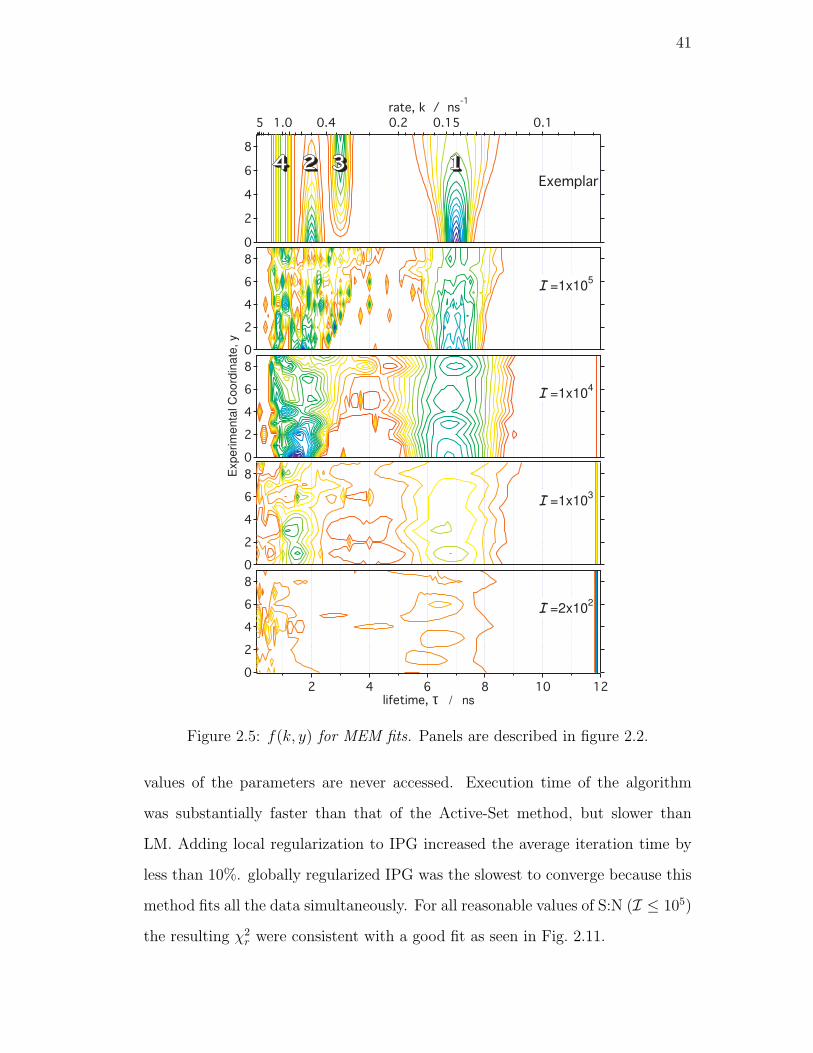
41
8
6
4
2
0
12108642lifetime, τ / ns
8
6
4
2
0
8
6
4
2
0
Exp
erim
en
tal C
oo
rdin
ate
, y
8
6
4
2
0
8
6
4
2
0
5 1.0 0.4 0.2 0.15 0.1
rate, k / ns-1
44 22 33 11Exemplar
I =1x10⁵
I =1x10⁴
I =1x10³
I =2x10²
Figure 2.5: f(k, y) for MEM fits. Panels are described in figure 2.2.
values of the parameters are never accessed. Execution time of the algorithm
was substantially faster than that of the Active-Set method, but slower than
LM. Adding local regularization to IPG increased the average iteration time by
less than 10%. globally regularized IPG was the slowest to converge because this
method fits all the data simultaneously. For all reasonable values of S:N (I ≤ 105)
the resulting χ2r were consistent with a good fit as seen in Fig. 2.11.
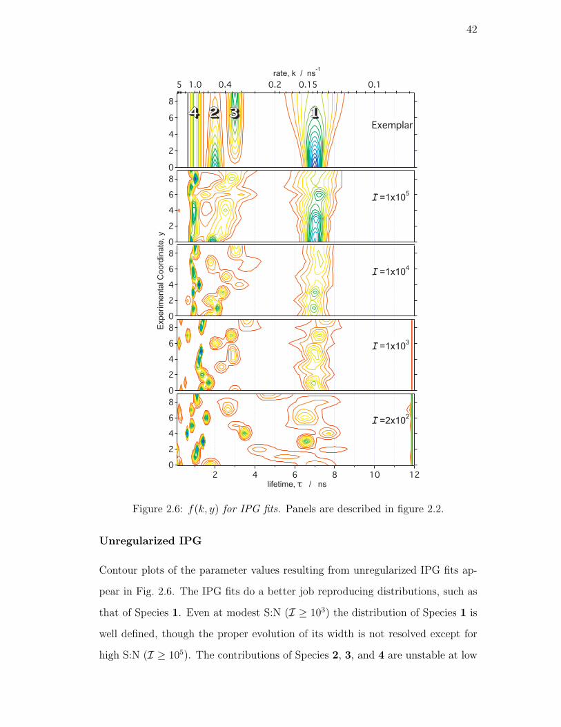
42
8
6
4
2
0
12108642 lifetime, t / ns
8
6
4
2
0
8
6
4
2
0
Experim
enta
l C
oord
inate
, y
8
6
4
2
0
8
6
4
2
0
5 1.0 0.4 0.2 0.15 0.1
rate, k / ns-1
44 22 33 11Exemplar
I =1x10⁵
I =1x10⁴
I =1x10³
I =2x10²
Figure 2.6: f(k, y) for IPG fits. Panels are described in figure 2.2.
Unregularized IPG
Contour plots of the parameter values resulting from unregularized IPG fits ap-
pear in Fig. 2.6. The IPG fits do a better job reproducing distributions, such as
that of Species 1. Even at modest S:N (I ≥ 103) the distribution of Species 1 is
well defined, though the proper evolution of its width is not resolved except for
high S:N (I ≥ 105). The contributions of Species 2, 3, and 4 are unstable at low

43
S:N.
At high S:N (I = 105) Species 4 is resolved from Species 2 and 3. However,
the conversion of Species 2 to 3 is a shifting distribution rather than separate
exchanging distributions. Only at the high S:N limit (I = 108 parameters not
shown) does the unregularized IPG method reproduce the contributions from all
four species and their evolution with y.
Even though population distributions are being reproduced, the species pop-
ulations for the IPG method evolve erratically over the experiment coordinate.
S1(y) decreases with y but the deviation from the exemplar, S1, is less than seen
in AS. S2(y) and S3(y) readily exchange population. S4(y) is far from constant
evolution across y.
Kullback-Liebler divergence systematically improves with increasing S:N. The
overall population parameter, POP , also improves with increasing S:N. Fitting
data with high S:N, I ≥ 2×10⁴, there is a big improvement in POP . Comparing
parameters in Fig. 2.6 with moderately-high to high S:N, i.e. I = 104 to I = 105,
IPG gains the ability to separate Species 2 from Species 3, albeit, with minimal,
success. To improve the IPG’s inability to accurately reproduce parameters at
low S:N, a regularizer may be used to stabilize the fitting procedure.
Locally Regularized IPG
The effect of the local regularizer on the fits can be seen in Fig. 2.7 as effectively
broadening the distributions as compared to unregularized IPG. The imposition
of the continuity condition in the transformed dimension k has essentially given
very similar solutions to that of the unmodified IPG except that the distributions
have broadened beyond the exemplar widths. At very low S:N, the correct trend
is impossible to ascertain in any reasonable way. Fitting moderate S:N data
(I = 104), the distribution of Species 1 is resolved but does not correctly evolve
in width. Concurrently, Species 2, 3 and 4 are merged into an undecipherable
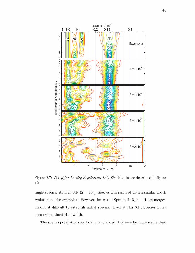
44
8
6
4
2
0
12108642 lifetime, t / ns
8
6
4
2
0
8
6
4
2
0
Exp
erim
en
tal C
oo
rdin
ate
, y
8
6
4
2
0
8
6
4
2
0
5 1.0 0.4 0.2 0.15 0.1
rate, k / ns-1
44 22 33 11Exemplar
I =1x10⁵
I =1x10⁴
I =1x10³
I =2x10²
Figure 2.7: f(k, y)for Locally Regularized IPG fits. Panels are described in figure2.2.
single species. At high S:N (I = 105), Species 1 is resolved with a similar width
evolution as the exemplar. However, for y < 4 Species 2, 3, and 4 are merged
making it difficult to establish initial species. Even at this S:N, Species 1 has
been over-estimated in width.
The species populations for locally regularized IPG were far more stable than
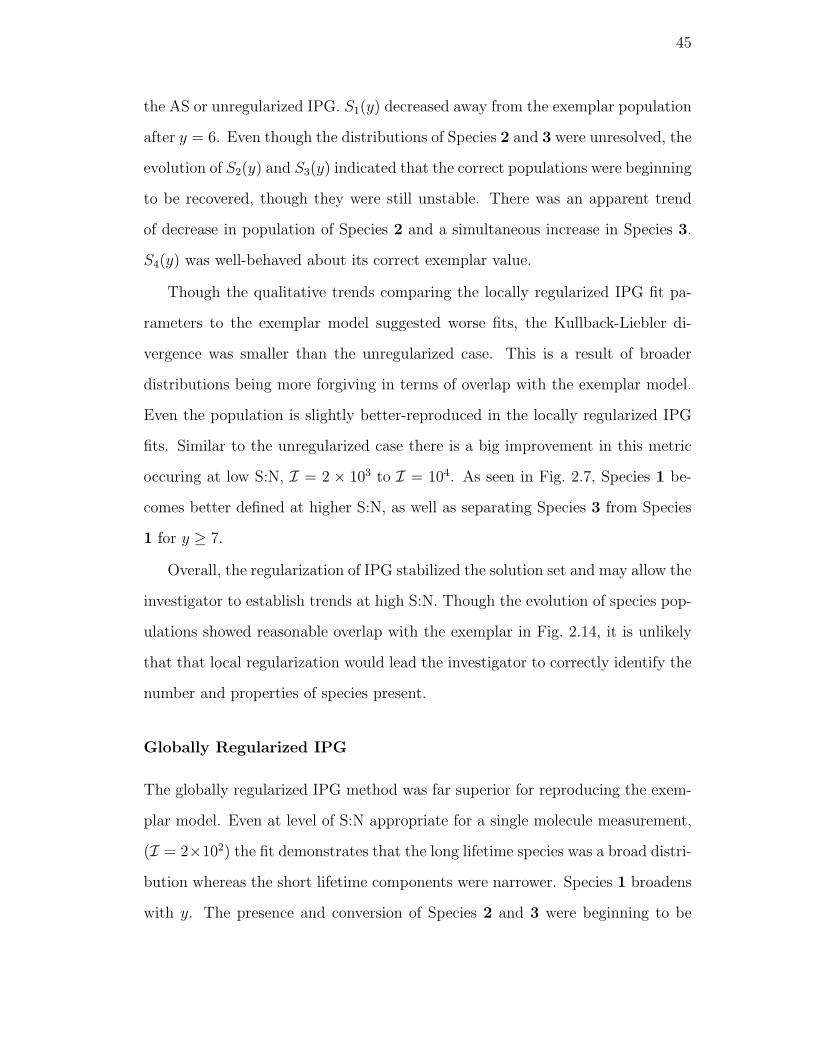
45
the AS or unregularized IPG. S1(y) decreased away from the exemplar population
after y = 6. Even though the distributions of Species 2 and 3 were unresolved, the
evolution of S2(y) and S3(y) indicated that the correct populations were beginning
to be recovered, though they were still unstable. There was an apparent trend
of decrease in population of Species 2 and a simultaneous increase in Species 3.
S4(y) was well-behaved about its correct exemplar value.
Though the qualitative trends comparing the locally regularized IPG fit pa-
rameters to the exemplar model suggested worse fits, the Kullback-Liebler di-
vergence was smaller than the unregularized case. This is a result of broader
distributions being more forgiving in terms of overlap with the exemplar model.
Even the population is slightly better-reproduced in the locally regularized IPG
fits. Similar to the unregularized case there is a big improvement in this metric
occuring at low S:N, I = 2 × 10³ to I = 104. As seen in Fig. 2.7, Species 1 be-
comes better defined at higher S:N, as well as separating Species 3 from Species
1 for y ≥ 7.
Overall, the regularization of IPG stabilized the solution set and may allow the
investigator to establish trends at high S:N. Though the evolution of species pop-
ulations showed reasonable overlap with the exemplar in Fig. 2.14, it is unlikely
that that local regularization would lead the investigator to correctly identify the
number and properties of species present.
Globally Regularized IPG
The globally regularized IPG method was far superior for reproducing the exem-
plar model. Even at level of S:N appropriate for a single molecule measurement,
(I = 2×10²) the fit demonstrates that the long lifetime species was a broad distri-
bution whereas the short lifetime components were narrower. Species 1 broadens
with y. The presence and conversion of Species 2 and 3 were beginning to be
46
8
6
4
2
0
12108642 lifetime, t / ns
8
6
4
2
0
8
6
4
2
0
Exp
erim
en
tal C
oo
rdin
ate
, y
8
6
4
2
0
8
6
4
2
0
5 1.0 0.4 0.2 0.15 0.1
rate, k / ns-1
44 22 33 11Exemplar
I =1x10⁵
I =1x10⁴
I =1x10³
I =2x10²
Figure 2.8: f(k, y) for Globally Regularized IPG fits. Panels are described infigure 2.2.
resolved. At modest S:N (I = 103), Species 2 and Species 3 were clearly two sep-
arate populations converting from one to the other, adjacent to a third constant
Species 4. The mean of the population distribution of Species 1 was about 7 ns,
increasing in width along the experimental coordinate.
The species population evolution was quite similar to that of the exemplar.
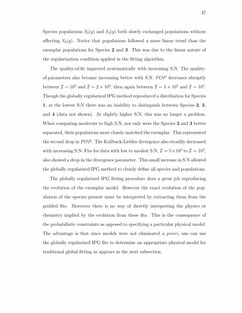
47
Species populations S2(y) and S3(y) both slowly exchanged populations without
affecting S4(y). Notice that populations followed a more linear trend than the
exemplar populations for Species 2 and 3. This was due to the linear nature of
the regularization condition applied in the fitting algorithm.
The quality-of-fit improved systematically with increasing S:N. The quality-
of-parameters also became increasing better with S:N. POP decreases abruptly
between I = 102 and I = 2× 10², then again between I = 5× 10³ and I = 104.
Though the globally regularized IPG method reproduced a distribution for Species
1, at the lowest S:N there was an inability to distinguish between Species 2, 3,
and 4 (data not shown). At slightly higher S:N, this was no longer a problem.
When comparing moderate to high S:N, not only were the Species 2 and 3 better
separated, their populations more closely matched the exemplar. This represented
the second drop in POP . The Kullback-Liebler divergence also steadily decreased
with increasing S:N. Fits for data with low to modest S:N, I = 5×10² to I = 103,
also showed a drop in the divergence parameter. This small increase in S:N allowed
the globally regularized IPG method to clearly define all species and populations.
The globally regularized IPG fitting procedure does a great job reproducing
the evolution of the exemplar model. However the exact evolution of the pop-
ulation of the species present must be interpreted by extracting them from the
gridded fits. Moreover there is no way of directly interpreting the physics or
chemistry implied by the evolution from these fits. This is the consequence of
the probabilistic constraints as opposed to specifying a particular physical model.
The advantage is that since models were not eliminated a priori, one can use
the globally regularized IPG fits to determine an appropriate physical model for
traditional global fitting as appears in the next subsection.

48
2.4.5 Global Model LM
A global model puts deterministic constraints on the model space in the trans-
formed coordinate. We determined a global fitting model using the distribution
of rates from the globally regularized IPG fit at I = 104 in Fig. 2.8. From this
fit, it is clear that there are four species. Species 1 had a significant width, that
slightly evolved and was centered at k−1= 7 ns. Conventional global fitting might
treat this as a stretched exponential expression (second term in Eq. 2.17) in order
to model a distribution of rates. Both the stretch parameter, β(y) and the rate
parameter, k1(y) must be local parameters since β(y) changes not only the width
of the distribution but also the mean.
The global fit also showed that Species 2, 3 and 4 were fairly narrow dis-
tributions thus represented by single exponentials, each with global rates, k2, k3
and k4. Though the populations of these species had fairly consistent trends (i.e.
Species 2 descended, 3 ascended and 4 remained nearly a constant in amplitude)
the model was kept general enough to allow variability in populations across the
evolution, by employing local pre-exponential factors P2(y), P3(y), P4(y), respec-
tively. The fit model also contained a baseline term, F0(y), local for each data
transient.
Part of the instability of non-linear least-squares fitting of multi-exponential
functions arises from the lack of constraints on the the exponential parameters.
Even with the proper discrete global model, the fit procedure must be constrained.
If they are left unconstrained, the exponential parameters can attain the same
values. When this occurs, singular matrix errors are encountered by the LM
algorithm causing the fit to fail. To forbid the global rate parameters from com-
bining, a problem common with non-linear multi-exponential fitting, constraints
were used. Constraints were placed upon global parameters, k2, k3, and k4, and
they were chosen based on the trends in the I = 104 globally regularized fits.
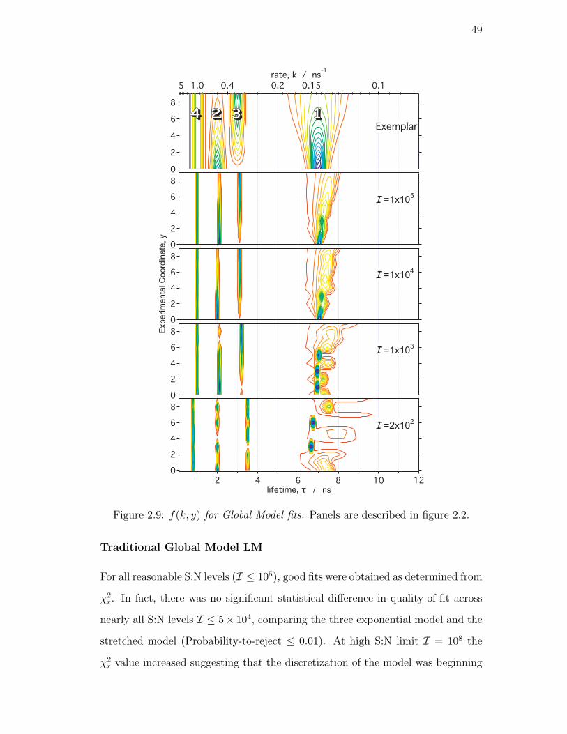
49
8
6
4
2
0
12108642lifetime, t / ns
8
6
4
2
0
8
6
4
2
0
Exp
erim
en
tal C
oo
rdin
ate
, y
8
6
4
2
0
8
6
4
2
0
5 1.0 0.4 0.2 0.15 0.1
rate, k / ns-1
44 22 33 11Exemplar
I =1x10⁵
I =1x10⁴
I =1x10³
I =2x10²
Figure 2.9: f(k, y) for Global Model fits. Panels are described in figure 2.2.
Traditional Global Model LM
For all reasonable S:N levels (I ≤ 105), good fits were obtained as determined from
χ2r. In fact, there was no significant statistical difference in quality-of-fit across
nearly all S:N levels I ≤ 5× 10⁴, comparing the three exponential model and the
stretched model (Probability-to-reject ≤ 0.01). At high S:N limit I = 108 the
χ2r value increased suggesting that the discretization of the model was beginning

50
to make a difference in the quality of the fit at that limit. For all S:N, fits were
robust but at low S:N, I ≤ 2 × 10², the global rates were often limited by the
constraint (not all data is shown).
For the low S:N fits, the stretched exponential term was not able to consis-
tently reproduce the Species 1 distribution. The β(y) parameter converged to
1 in several cases resulting in a discrete exponential for some values of y. Even
though Species 1, 2 and 3 were centered at nearly the correct lifetime, the local
amplitudes fluctuate greatly at low S:N. By a moderate S:N level, I = 104, the
fits nicely reproduce the width and evolution of the Species 1 distribution. The
instability of the β parameter for the fit to Species 1 appeared to interfere with
the fitting of the conversion of Species 2 to 3, which was not correctly reproduced
until I = 104. The Species 4 region was properly reproduced even at low S:N,
I = 2× 10².
As anticipated, the ability of the global model to reproduce the populations
was excellent. The populations trends appeared to be only slightly “noisy” across
y. Moreover, the POP metric shows global model thus far producing the best
overlap with each species population from I ≥ 5 × 10². Because all population
for a particular species were determined from subranges of the grid of k’s, the
POP parameter was less sensitive to the discrete nature of model used to describe
Species 2, 3 and 4. The plateau in DKL divergence at I ∼ 104 suggests that above
this value the deterministic constraints on the transformed coordinate dimensions
of the model space limit the quality of overlap with the exemplar model.
The local nature of the amplitude parameters allowed them to fluctuate greatly
along y, especially for low to modest S:N. A specific deterministic model along y
related to some physical theory could help stabilize this situation. We note that
since there was no improvement in Kullback-Liebler divergence or POP for high
S:N limit (I = 108), we expect little gain in parameter stability at moderately
high S:N (I > 104) with a regularized model. Nonetheless, in the spirit of first
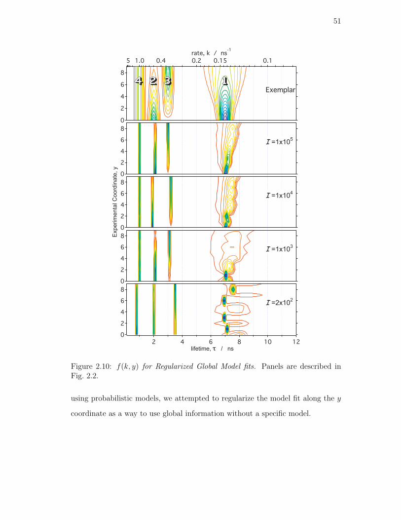
51
8
6
4
2
0
12108642 lifetime, t / ns
8
6
4
2
0
8
6
4
2
0
Experim
enta
l C
oord
inate
, y
8
6
4
2
0
8
6
4
2
0
5 1.0 0.4 0.2 0.15 0.1
rate, k / ns-1
44 22 33 11Exemplar
I =1x10⁵
I =1x10⁴
I =1x10³
I =2x10²
Figure 2.10: f(k, y) for Regularized Global Model fits. Panels are described inFig. 2.2.
using probabilistic models, we attempted to regularize the model fit along the y
coordinate as a way to use global information without a specific model.

52
Regularized Global Model LM
Regularization of the global LM fitting increased convergence time by no more
than a factor of 2 and increased the stability of the fitting procedure. The values
of χ2r indicated good fits across all reasonable values S:N and were not statisti-
cally different from the traditional global model fits as measured by the F-test
(probability-to-reject < 0.05).
The addition of the regularizer stabilizes the distribution due to Species 1.
This, in turn, stabilized the evolution of Species 2 and 3 since Species 1 was no
longer interfering with them. Overall good fits were obtained at moderate S:N
I ≥ 103.
The globally regularized model fit was a considerably better method for re-
producing the distribution of Species 1 at very low S:N. Species 1 had a clear
distribution across the experimental coordinate, but lacked an evolving trend in
width. Species 2, 3 and 4 had the correct population trends but are close to
the employed bounds. For data with I ≥ 103, all species were well within the
imposed bounds, while showing an evolving width associated with Species 1. The
ability of this method to resolve Species 2, 3 and 4 did not change much with
increasing S:N I ≥ 103, while Species 1 improved with better S:N.
The addition of the regularizer to an otherwise traditional global fit improved
the ability of the fit to reproduce systematic changes in species population evo-
lution as seen in Fig. 2.14. Specifically, the evolutions for the regularized global
model were noticeably smoother. As with the globally regularized IPG fits, S2(y)
and S3(y) were more linear than their respective exemplar evolutions. The con-
stant species, S4(y), also did not have a consistent increasing trend, as it did
for the globally regularized IPG. Though S1(y) was slightly overestimated, the
population evolution was nearly constant.
53
The match with the exemplar model was limited because of the discrete char-
acter of the model in the transformed dimension as seen in the Kullback-Liebler
divergence. However, when comparing the Kullback-Liebler divergence for the
regularized global model fits to the traditional global model, the regularizer model
reached a plateau sooner (I = 103 versus I = 5 × 10³). As seen in Fig. 2.9 and
Fig. 2.10, the regularized global model stabilized the evolving distribution of
Species 1 with modest S:N, I = 103. There was no improvement in Kullback-
Liebler divergence in the high S:N limit(I = 108).
The POP metric steadily decreased until a plateau was reached for moderate
S:N, I = 2 × 10³. This indicated that from a species population point-of-view,
nothing else can be gained from better S:N. This can be seen in the increase in
the POP value for fits to the highest S:N data (I = 108), thereby showing the
addition of a regularizer is not necessary for a discrete global model fit to virtually
infinite S:N data.
2.5 Discussion
2.5.1 Comparison of Methods
In the results we evaluated how the S:N ratio influenced the success of each
fitting method using χ2r, the Kullback-Liebler divergence, and the population
parameters. We now compare the different methods to each other and discuss
why they gave different results.
Reduced Chi-square
The four deterministically constrained models (all optimized with LM) showed
little systematic change in χ2r until I ≥ 5 × 10⁴, at which point χ2
r began to
get worse. By comparison, the gridded methods (optimized by AS, MEM, or
IPG) showed steady improvement in χ2r until I = 105. There was no statistical

54
difference of fit between the AS fit and any of the MEM or IPG fits except in
the high S:N limit (I = 108). The MEM fits gave slightly higher χ2r because of
the higher value of the regularizer strength parameter required to get reasonable
fits. One interpretation of the higher χ2r for the gridded methods would be that
they were done on too coarse of a grid. However, the improvement in χ2r with
increasing S:N suggests otherwise, since a constraint in the model space would
be reflected as a lower boundary for the χ2r. Furthermore, improving the grid
resolution did not change χ2r. Grid methods have more model flexibility and can
take advantage of the increased S:N, however the model space they are performed
in does not include terms that adapt to the noise.
The global model fits were not statistically different than the three exponential
fits until they began to diverge in terms of χ2r at I > 104 because they have less
model flexibility than three exponential and four exponential fits. According to
χ2r the three exponential model was adequate to describe the data for these fits
until high S:N. In the high S:N limit it was quite clear that neither the three nor
the four exponential fit was a good model for the system.
Kullback-Liebler divergence
The Kullback-Liebler divergences comparing the exemplar parameters to the three
exponential, four exponential, AS, global model and regularized global model
fits did not improve much with increasing signal-to-noise. (See Fig. 2.12) The
deterministic constraints implied by these fitting methods forbid the true solution.
At low S:N (I = 102) the methods were all clustered. In this limit the AS
method was worst and the three exponential model was best. This suggests that
too much model flexibility is not good when the there is little information in the
data, as the model flexibility will be used to fit noise. The MEM and IPG methods
did a better job than AS because they tended to give continuous distributions
that better represented the broad part of Species 1 and were less able to adapt
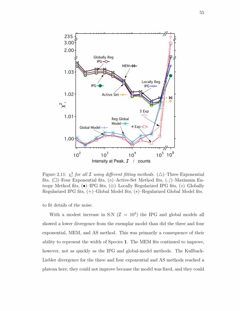
55
1.03
1.02
1.01
1.00
χ2
r
102
103
104
105
Intensity at Peak, I / counts
3.00
2.00
108
235
Globally RegIPG
IPGLocally Reg
IPG
Active Set
Global Model
Reg Global
Model4 Exp
3 Exp
MEM
Figure 2.11: χ2r for all I using different fitting methods. (4)–Three Exponential
fits, ()–Four Exponential fits, ()–Active-Set Method fits, (./)–Maximum En-tropy Method fits, (•)–IPG fits, (⊗)–Locally Regularized IPG fits, ()–GloballyRegularized IPG fits, (+)–Global Model fits, (∗)–Regularized Global Model fits.
to fit details of the noise.
With a modest increase in S:N (I = 103) the IPG and global models all
showed a lower divergence from the exemplar model than did the three and four
exponential, MEM, and AS method. This was primarily a consequence of their
ability to represent the width of Species 1. The MEM fits continued to improve,
however, not as quickly as the IPG and global-model methods. The Kullback-
Liebler divergence for the three and four exponential and AS methods reached a
plateau here; they could not improve because the model was fixed, and they could
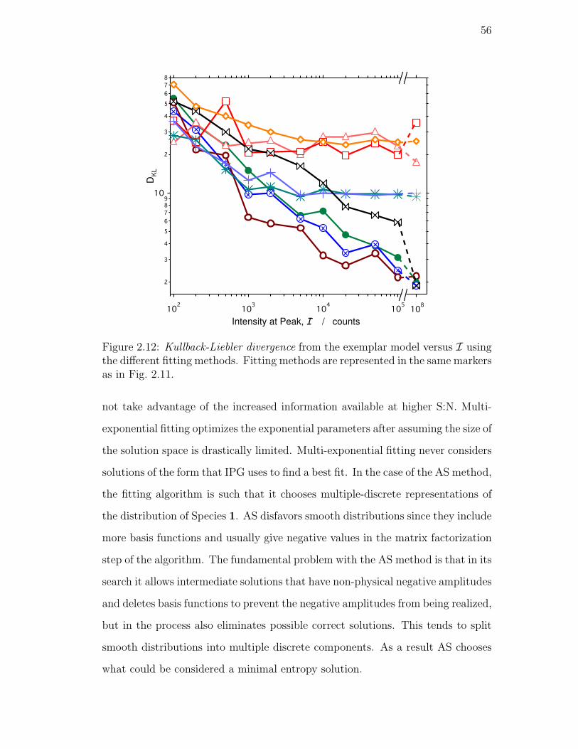
56
2
3
4
5
6
7
89
10
2
3
4
5
6
7
8
DK
L
108
102
103
104
105
Intensity at Peak, I / counts
Figure 2.12: Kullback-Liebler divergence from the exemplar model versus I usingthe different fitting methods. Fitting methods are represented in the same markersas in Fig. 2.11.
not take advantage of the increased information available at higher S:N. Multi-
exponential fitting optimizes the exponential parameters after assuming the size of
the solution space is drastically limited. Multi-exponential fitting never considers
solutions of the form that IPG uses to find a best fit. In the case of the AS method,
the fitting algorithm is such that it chooses multiple-discrete representations of
the distribution of Species 1. AS disfavors smooth distributions since they include
more basis functions and usually give negative values in the matrix factorization
step of the algorithm. The fundamental problem with the AS method is that in its
search it allows intermediate solutions that have non-physical negative amplitudes
and deletes basis functions to prevent the negative amplitudes from being realized,
but in the process also eliminates possible correct solutions. This tends to split
smooth distributions into multiple discrete components. As a result AS chooses
what could be considered a minimal entropy solution.
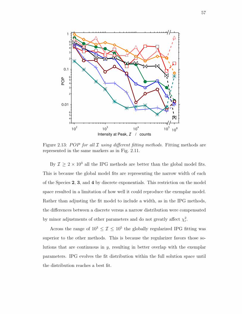
57
3
4
56
0.01
2
3
4
56
0.1
2
3
4
56
1
PO
P
102
103
104
105
Intensity at Peak, I / counts10
8
Figure 2.13: POP for all I using different fitting methods. Fitting methods arerepresented in the same markers as in Fig. 2.11.
By I ≥ 2 × 10³ all the IPG methods are better than the global model fits.
This is because the global model fits are representing the narrow width of each
of the Species 2, 3, and 4 by discrete exponentials. This restriction on the model
space resulted in a limitation of how well it could reproduce the exemplar model.
Rather than adjusting the fit model to include a width, as in the IPG methods,
the differences between a discrete versus a narrow distribution were compensated
by minor adjustments of other parameters and do not greatly affect χ2r.
Across the range of 103 ≤ I ≤ 105 the globally regularized IPG fitting was
superior to the other methods. This is because the regularizer favors those so-
lutions that are continuous in y, resulting in better overlap with the exemplar
parameters. IPG evolves the fit distribution within the full solution space until
the distribution reaches a best fit.
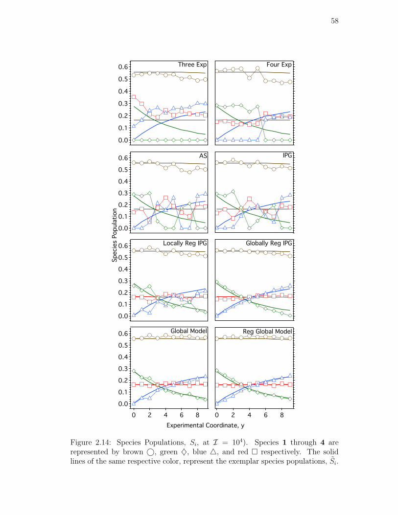
58
0.6
0.5
0.4
0.3
0.2
0.1
0.0
8642086420
Experimental Coordinate, y
0.6
0.5
0.4
0.3
0.2
0.1
0.0
0.6
0.5
0.4
0.3
0.2
0.1
0.0
Specie
s Popula
tion
0.6
0.5
0.4
0.3
0.2
0.1
0.0
Locally Reg IPG
AS
Three Exp Four Exp
IPG
Globally Reg IPG
Reg Global ModelGlobal Model
Figure 2.14: Species Populations, Si, at I = 104). Species 1 through 4 arerepresented by brown ©, green ♦, blue 4, and red respectively. The solidlines of the same respective color, represent the exemplar species populations, Si.

59
Population Evolution
The POP parameter in Fig. 2.13 measures the overall ability of the fit to extract
the evolution of the populations, while the individual populations of the different
species appear in Fig. 2.14. The globally regularized IPG began improving at a
lower signal level than the other IPG methods, however at higher signal levels
the other methods eventually caught up. The MEM fits were comparable to the
locally regularized fits for low S:N but after I = 2× 10³ the MEM was worse and
did not catch up until the higher accuracy of our MEM implementation became
important in the high S:N limit (I = 108)). The global regularizer could not do
a perfect job tracking the population evolution because it inherently measures
deviation from a linear dependence of the evolution in y. As a result the evolu-
tion was “flatter” than it should have been as shown in Fig. 2.14 right column,
third row. Once it is known that there are a certain number of species and that
they are evolving, the regularizer could be modified to allow more curvature in
the evolution by measuring departure from piecewise quadratic behavior with a
third derivative regularizer. However at the level of reconstruction afforded by
the second-order global regularizer, one would be better served forming a phe-
nomenological model describing the evolution and fitting to that global model to
extract physical parameters from the data.[7] Prior knowledge in this case arises
from the formation of a physical hypothesis and allows the global models to get a
better solution. The traditional global model and regularized global model illus-
trate this point as they both did an excellent job reconstructing the populations
and their evolution.
2.5.2 Prior Knowledge and Probabilistic Constraints
For all reasonable S:N levels, an investigator considering the value of χ2r and the F-
test would be led to choose the three exponential model. If one also considered the
60
details of the experiment and used that prior knowledge in the fitting procedure
one would obtain better results in terms of identification of the species present,
their properties in terms of the transformed coordinate, k, as well as evolution
of their populations across the non-transformed coordinate, y. Stabilization by
global fitting works because the model space is being limited. To start with
a deterministic global model would be to start with an assumed answer and
eliminate all other regions of model space.
We saw how the addition of a regularization condition in the transformed
dimension, k, perturbs not only the narrow distributions of Species 2, 3, and 4
but also increases the width of the broad distribution of Species 1. The broadening
from the regularizer masked the evolution of the Species 1 width. We see that
the regularized IPG gave fits that were no better and were in some ways worse
than than those given by unregularized IPG. This is because the transformed-
coordinate regularizer is adding incorrect information to the fitting procedure.
In the case of the three exponential, four exponential, and AS fitting there
was also incorrect information being added to the fitting procedure. In the case
of the three and four exponential fits, the incorrect information was that the
distributions are discrete. This limits the solution space available for the fits to
the point where no correct solution can be found because the correct solution is
not included in the space of possible solutions. The space of possible solutions
for the AS method fits includes the correct solution, however the search space
includes solutions that are not in the space of possible solutions. The algorithmic
mechanism used to return the search from the forbidden space to the allowed
space is what biases the fit away from the correct solution. In locally regularized
IPG the local solutions are biased away from solutions that include discrete or
sharp features and thus, though the available solution space includes the correct
solution, the regularizer puts an a-priori bias against it because it includes narrow
features. When viewed in this light, it is understandable why regularization in
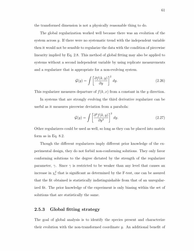
61
the transformed dimension is not a physically reasonable thing to do.
The global regularization worked well because there was an evolution of the
system across y. If there were no systematic trend with the independent variable
then it would not be sensible to regularize the data with the condition of piecewise
linearity implied by Eq. 2.8. This method of global fitting may also be applied to
systems without a second independent variable by using replicate measurements
and a regularizer that is appropriate for a non-evolving system.
G(y) =
∫ [∂f(k, y)
∂y
]2
dy. (2.26)
This regularizer measures departure of f(k, x) from a constant in the y direction.
In systems that are strongly evolving the third derivative regularizer can be
useful as it measures piecewise deviation from a parabola:
G(y) =
∫ [∂3f(k, y)
∂y3
]2
dy. (2.27)
Other regularizers could be used as well, so long as they can be placed into matrix
form as in Eq. 8.2.
Though the different regularizers imply different prior knowledge of the ex-
perimental design, they do not forbid non-conforming solutions. They only favor
conforming solutions to the degree dictated by the strength of the regularizer
parameter, γ. Since γ is restricted to be weaker than any level that causes an
increase in χ2r that is significant as determined by the F-test, one can be assured
that the fit obtained is statistically indistinguishable from that of an unregular-
ized fit. The prior knowledge of the experiment is only biasing within the set of
solutions that are statistically the same.
2.5.3 Global fitting strategy
The goal of global analysis is to identify the species present and characterize
their evolution with the non-transformed coordinate y. An additional benefit of
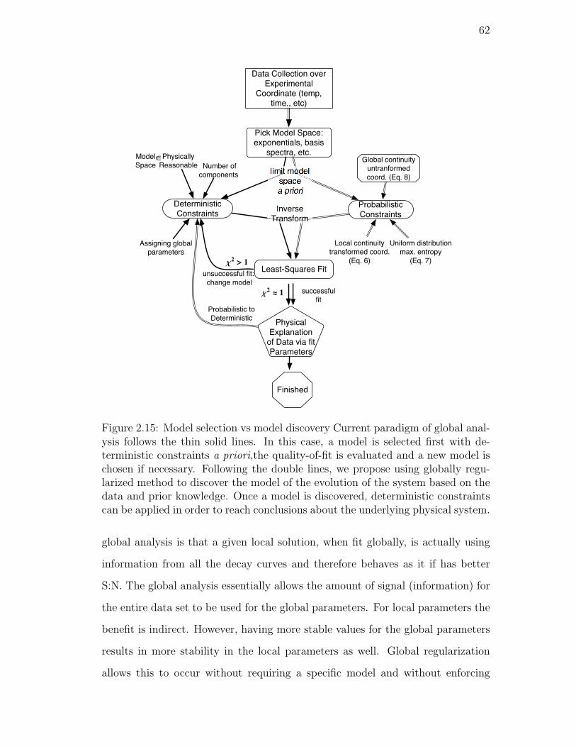
62
Finished
Pick Model Space:exponentials, basis
spectra, etc.
DeterministicConstraints
ProbabilisticConstraints
Local continuity
transformed coord.
(Eq. 6)
Physical Explanation of Data via fit Parameters
Global continuity
untranformed
coord. (Eq. 8)
Uniform distribution
max. entropy
(Eq. 7)
Least-Squares Fit
Probabilistic to
Deterministic
limit modelspacea priori
InverseTransform
Number of
components
Assigning global
parameters
Physically
Reasonable
Model
Space ∈
unsuccessful fit:
change modelsuccessful
fitΧ2" 1
Χ2" 1
Data Collection overExperimental
Coordinate (temp, time., etc)
Figure 2.15: Model selection vs model discovery Current paradigm of global anal-ysis follows the thin solid lines. In this case, a model is selected first with de-terministic constraints a priori,the quality-of-fit is evaluated and a new model ischosen if necessary. Following the double lines, we propose using globally regu-larized method to discover the model of the evolution of the system based on thedata and prior knowledge. Once a model is discovered, deterministic constraintscan be applied in order to reach conclusions about the underlying physical system.
global analysis is that a given local solution, when fit globally, is actually using
information from all the decay curves and therefore behaves as it if has better
S:N. The global analysis essentially allows the amount of signal (information) for
the entire data set to be used for the global parameters. For local parameters the
benefit is indirect. However, having more stable values for the global parameters
results in more stability in the local parameters as well. Global regularization
allows this to occur without requiring a specific model and without enforcing

63
a value on a global parameter. Even when a traditional global model is used a
regularizer can allow partial globalization of the non-global parameters. The non-
global parameters are essentially free of the model. In the present example the
global model would have needed to be expanded to include a specific functional
form for the evolution of the population parameters.
Fig. 2.15 illustrates a fitting strategy that step-wise reduces the available
model space according to the data and prior knowledge. This allows fitting of
the global data set without sacrificing the range of the model space while still
allowing quantitative conclusions to be drawn. Initially one should use prior
knowledge to determine the range of valid k for the inversion. Alternatively this
could be done with a traditional multi-exponential LM fit or a large-grid AS
fit. Once the model space has been identified, one should use prior knowledge
of the experimental design to determine if there should be some expectation of
continuity or other regularization condition in either or both of the coordinates
k and y. Once a probabilistically constrained model space is available, one can
perform a global fit that includes all the model space using the globally regularized
IPG method. From the globally regularized IPG fits one should identify the
species present and form a deterministically constrained global model for the
transformed (species) coordinate. A traditional global model can then fit the
data either with or without a probabilistic constraint on the non-transformed
(evolution) coordinate. At this point a global model for both coordinates should
be apparent and further reduction based on a fully deterministic physical model
with a small number of parameters should be feasible.
64
2.6 Conclusions
Current physical measurements include complex systems that do not give simple
homogeneous signals. Large heterogeneous data sets measured over many con-
ditions have become the norm. Extracting physical information from such data
sets requires handling large model spaces in the fitting procedure. Fitting with
large numbers of basis functions such as is done in this work has only recently
become feasible. The complexity of the global regularization method would have
been prohibitive given the computational facilities commonly available 10 years
ago. Many of the assumptions for approaches to and algorithms for data fitting
and reduction were shaped by technological limitations of 20 or more years ago.
Modern computers allow direct fitting of large data sets and should be exploited
to allow better insight into the processes behind the data.
65
References
[1] B. Alberts. The cell as a collection of protein machines: preparing the nextgeneration of molecular biologists. Cell, 92:291–294, 1998.
[2] Joanna Kaylor, Nika Bodner, Shauna Edridge, Ghiam Yamin, Dong-PyoHong, and Anthony L. Fink. Characterization of oligomeric intermediatesin [alpha]-synuclein fibrillation: Fret studies of y125w/y133f/y136f [alpha]-synuclein. Journal of Molecular Biology,, 353:357–372, 2005.
[3] James H. Werner, Raymond Joggerst, R. Brian Dyer, and Peter M. Goodwin.A two-dimensional view of the folding energy landscape of cytochrome c.Proceedings of the National Academy of Sciences, 103(30):11130–11135, 2006.
[4] H Frauenfelder, SG Sligar, and PG Wolynes. The energy landscapes andmotions of proteins. Science, 254(5038):1598–1603, 1991.
[5] Buyong Ma and Ruth Nussinov. The stability of monomeric intermediatescontrols amyloid formation: Abeta25-35 and its n27q mutant. BiophysicalJournal, 90(10):3365–3374, 2006.
[6] Atta Ahmad, Vladimir N. Uversky, Dongpyo Hong, and Anthony L. Fink.Early events in the fibrillation of monomeric insulin. J. Biol. Chem.,280(52):42669–42675, 2005.
[7] Troy C. Messina and David. S. Talaga. Free energy landscapes remodeledby ligand binding. Biophysical Journal, 93:579–585, 2007.
[8] Jeremy Pronchik and David S. Talaga. Separation and analysis of dynamicstokes shift with multiple fluorescence environments: Coumarin 153 in bovine-lactoglobulin a. In Preparation, 2007.
[9] Ashok A. Deniz, Samrat Mukhopadhyay, and Edward A. Lemke. Single-molecule biophysics: at the interface of biology, physics and chemistry. J. R.Soc. Interface, FirstCite Early Online Publishing:1–31, 2007.
[10] F. Ritort. Single-molecule experiments in biological physics: methods andapplications. Journal of Physics: Condensed Matter, 18, 2006.
[11] H. Peter Lu, Luying Xun, and X. Sunney Xie. Single-molecule enzymaticdynamics. Science, 282(5395):1877–1882, 1998.
66
[12] David S. Talaga, Wai Leung Lau, Heinrich Roder, Jianyong Tang, Yiwei Jia,William F. DeGrado, and Robin M. Hochstrasser. Dynamics and folding ofsingle two-stranded coiled-coil peptides studied by fluorescent energy transferconfocal microscopy. Proceedings of the National Academy of Sciences of theUnited States of America, PNAS:13021 – 13026, 2000.
[13] W. Miller and K. A. Dill. Ligand binding to proteins: The binding landscapemodel. Protein Science, 6:2166–2179, 1997.
[14] Laura D’Alfonso, Maddalena Collini, and Giancarlo Baldini. Does beta-lactoglobulin denaturation occur via an intermediate state? Biochemistry,41:326–333, 2002.
[15] Xianglan He & David S. Talaga Jason T. Giurleo. Nonspecific aggregationis the first step in -lactoglobulin amyloid formation. In Preparation, 2007.
[16] E. T. Jaynes. Probability Theory: The Logic of Science. Cambridge univ.Press, Cambridge, 2003.
[17] Stephen W. Provencher. A contrained regularization method for invertingdata represented by linear algebraic or integral equations. Computer PhysicsCommunications, 27:213–227, 1982.
[18] Various Authors. Dynamic light scattering, the method and some applica-tions, 1993.
[19] B. J. Berne and R. Pecora. Dynamic Light Scattering. Wiley, New York,1976.
[20] A. K. Livesey, P. Licinio, and M. Delaye. Maximum entropy analysis ofquasielastic light scattering from colloidal dispersions. Journal ChemicalPhysics, 84:5102–5107, 1986.
[21] Stephen W. Provencher and Jurgen Glockner. Estimation of globular proteinsecondary structure from circular dichroism. Biochemistry, 20:33–37, 1981.
[22] S. Sibisi. Two-dimensional reconstructions from one-dimensional data bymaximum entropy. Nature, 301:134–136, 1983.
[23] A. K. Livesey and J. C. Brochon. Analyzing the distribution of decay con-stants in pulse-fluorimetry using the maximum entropy method. BiophysicalJournal, 52:693–706, 1987.
[24] Emil Post. Generalized differentiation. Trans. Amer. Math. Soc., 32:723–781., 1930.
[25] Albert Tarantola. Inverse Problem Theory and Methods for Model Param-eter Estimation. SIAM: Society for Industrial and Applied Mathematics,December 2004.
67
[26] William Press, Saul Teukolsky, William Vetterling, and Brian Flannery. Nu-merical Recipes in C. Cambridge University Press, Cambridge, UK, 2ndedition, 1992.
[27] J. G. McWhirter and E. R. Pike. On the numerical inversion of the laplacetransform and similar fredholm integral equations of the first kind. J. Phys.A Math. Gen., 11:1729–1745, 1978.
[28] K Levenberg. A method for the solution of certain problems in least squares.Quarterly of Applied Mathematics, 2:164–168, 1944.
[29] D Marquardt. An algorithm for least-squares estimation of nonlinear param-eters. SIAM, Journal of Applied Mathematics, 11:431–441, 1963.
[30] Andrey N. Tikhonov and Vasiliy Y. Arsenin. Solutions of ill-posed problem.Wiley, New York, 1977.
[31] Charles L. Lawson and Richard J. Hanson. Solving Least Squares Problems.Prentice-Hall, Inc., 1974.
[32] M. Merritt and Y. Zhang. An interior-point gradient method for large-scaletotally nonnegative least squares problems. Journal of Optimization Theoryand Applications, 126:191–202, 2005.
[33] Mark H.Van Benthem and Michael R. Keenan. Fast algorithm for the solu-tion of large-scale non-negativity-constrained least squares problems. Jour-nal of Chemmetrics, 18:441?450, 2004.
[34] J. B. Rosen. The gradient projection method for nonlinear programming.part i. linear constraints. Journal of the Society for Industrial and AppliedMathematics, 8:181–217, 1960.
[35] A. A. Goldstein. Convex programming in hilbert space. Bulletin of theAmerican Mathematical Society, 70:709–710, 1964.
[36] Aleksander Siemiarczuk, Brian D. Wagner, and William R. Ware. Compari-son of the maximum entropy and exponential series methods for the recoveryof distributions of lifetimes from fluorescence lifetime data. The Journal ofPhysical Chemistry, 94:1661 – 1666, 1990.
[37] Douglas R. James and William R.. Ware. A fallacy in the interpretation offluorescence decay parameters. Chemical Physics Letters, 120:455–9, 1985.
[38] Alexander P. Demchenko, Michel Vincent, and Jacques Gallay. Solvent re-laxation around the excited state of indole: Analysis of fluorescence lifetimedistributions and time-dependence spectral shifts. Journal Physical Chem-istry, 99:14931–14941, 1995.

68
[39] Gufeng Wang, Yi Gao, and M. Lei Geng. Analysis of heterogeneousfluorescence decays in proteins. using fluorescence lifetime of 8-anilino-1-naphthalenesulfonate to probe apomyoglobin unfolding at equilibrium.Biochimica et Biophysica Acta, 1760:1125 –1137, 2006.
[40] D.S. Jones. Elementary Information Theory. Oxford: Oxford UniversityPress., 1979.
[41] J. Ricardo Alcala, Enrico Gratton, and Franklyn G. Prendergast. Fluores-cence lifetime distributions in proteins. Biophysical Journal, 51:597–604,1987.
[42] J. Ricardo Alcala, Enrico Gratton, and Franklin G. Prendergast. Interpreta-tion of fluorescence decays in proteins using continuous lifetime distributions.Biophysical Journal, 51:925–936, 1987.
[43] Graham Hungerford and David J. S. Birch. Single-photon timing detectorsfor fluorescence lifetime spectroscopy. Measurement Science & Technology,7:121–35, 1996.

69
Chapter 3
β-Lactoglobulin Assembles into Amyloid
through Sequential Aggregated Intermediates
3.1 Summary
We have investigated the aggregation and amyloid fibril formation of bovine β-
lactoglobulin variant A with a focus on the early stages of aggregation. We used
time-resolved non-covalent labeling with thioflavin T and 1-anilino-8-naphthalenesulfonate
to follow the conformational changes occurring in β-lactoglobulin during aggre-
gation. 1-anilino-8-naphthalenesulfonate monitored the involvement of the hy-
drophobic core/calyx of β-lactoglobulin in the aggregation process. Thioflavin T
luminescence monitored formation of amyloid. The luminescence lifetime distri-
butions of both probes showed changes that could be attributed to conformational
changes occurring during and following aggregation. To correlate the lumines-
cence measurements with the degree of aggregation and the morphology of the
aggregates, we also measured dynamic light scattering and atomic force micro-
scopic images. We evaluate the relative stability of the intermediates with an
assay sensitive to aggregation reversibility. Our results suggest that initial aggre-
gation during the first 5 days occurred with partial disruption of the characteristic
calyx in β-lactoglobulin. As the globular aggregates grew from days 5-16, the ca-
lyx was completely disrupted and the globular aggregates became more stable.
After this second phase of aggregation, conversion to a fibrillar form occurred
marking the growth phase and still more changes in the luminescence signals
were observed. Based on these observations we propose a three-step process by
70
which monomer is converted first to weakly-associated aggregates that rearrange
into stable aggregates that eventually convert to protofibrils that elongate in the
growth phase.
3.2 Introduction
3.2.1 Amyloid Formation
Aggregation of soluble polypeptides or proteins into insoluble amyloid fibrils
containing the cross-β structural motif has been observed in the progression of
over 20 diseases.[1] The human health impact of these diseases has motivated
intensive study and numerous reviews of the structure and growth of amyloid
fibrils.[1, 2, 3, 4, 5, 6, 7, 8, 9]
Amyloid formation often shows a sigmoidal kinetic growth pattern. Early
times are characterized by a lag phase where little or no fibrillar growth is ob-
served. The growth phase follows where amyloid rapidly assembles. The reaction
then slows with amyloid accumulation reaching a plateau.[10, 1, 11] After this
point amyloid often begins to gel or precipitate in vitro. The duration of the lag
phase and the growth phase both change dramatically depending on the incuba-
tion conditions.[12, 13, 14]
The kinetic lag phase for many amyloidogenic precursors is characterized by
conversion of soluble monomers to small oligomers.[15, 10, 14] One of the driving
forces for initial aggregation of soluble globular proteins may be the partitioning
of hydrophobic side chains into a central core, much like protein folding.[16] The
structural content and contribution to amyloid assembly of the small oligomers
is usually only inferred.[17, 18] During the lag phase there is little appreciable
amyloid formation as determined by histological assays. The lag time can be
reduced or eliminated by addition of mature amyloid as observed both in vivo,
by mortality of the organism and/or autopsy with histological staining [19], and
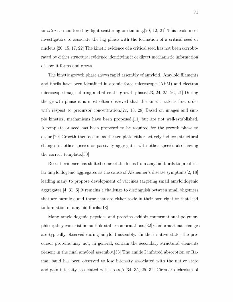
71
in vitro as monitored by light scattering or staining.[20, 12, 21] This leads most
investigators to associate the lag phase with the formation of a critical seed or
nucleus.[20, 15, 17, 22] The kinetic evidence of a critical seed has not been corrobo-
rated by either structural evidence identifying it or direct mechanistic information
of how it forms and grows.
The kinetic growth phase shows rapid assembly of amyloid. Amyloid filaments
and fibrils have been identified in atomic force microscope (AFM) and electron
microscope images during and after the growth phase.[23, 24, 25, 26, 21] During
the growth phase it is most often observed that the kinetic rate is first order
with respect to precursor concentration.[27, 13, 28] Based on images and sim-
ple kinetics, mechanisms have been proposed,[11] but are not well-established.
A template or seed has been proposed to be required for the growth phase to
occur.[29] Growth then occurs as the template either actively induces structural
changes in other species or passively aggregates with other species also having
the correct template.[30]
Recent evidence has shifted some of the focus from amyloid fibrils to prefibril-
lar amyloidogenic aggregates as the cause of Alzheimer’s disease symptoms[2, 18]
leading many to propose development of vaccines targeting small amyloidogenic
aggregates.[4, 31, 6] It remains a challenge to distinguish between small oligomers
that are harmless and those that are either toxic in their own right or that lead
to formation of amyloid fibrils.[18]
Many amyloidogenic peptides and proteins exhibit conformational polymor-
phism; they can exist in multiple stable conformations.[32] Conformational changes
are typically observed during amyloid assembly. In their native state, the pre-
cursor proteins may not, in general, contain the secondary structural elements
present in the final amyloid assembly.[33] The amide I infrared absorption or Ra-
man band has been observed to lose intensity associated with the native state
and gain intensity associated with cross-β.[34, 35, 25, 32] Circular dichroism of
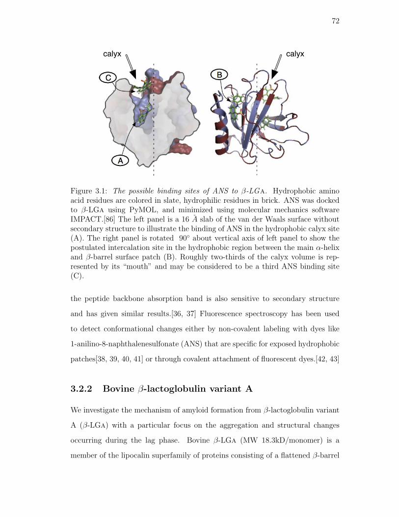
72
calyx calyx
A
C B
Figure 3.1: The possible binding sites of ANS to β-LGa. Hydrophobic aminoacid residues are colored in slate, hydrophilic residues in brick. ANS was dockedto β-LGa using PyMOL, and minimized using molecular mechanics softwareIMPACT.[86] The left panel is a 16 A slab of the van der Waals surface withoutsecondary structure to illustrate the binding of ANS in the hydrophobic calyx site(A). The right panel is rotated 90 about vertical axis of left panel to show thepostulated intercalation site in the hydrophobic region between the main α-helixand β-barrel surface patch (B). Roughly two-thirds of the calyx volume is rep-resented by its “mouth” and may be considered to be a third ANS binding site(C).
the peptide backbone absorption band is also sensitive to secondary structure
and has given similar results.[36, 37] Fluorescence spectroscopy has been used
to detect conformational changes either by non-covalent labeling with dyes like
1-anilino-8-naphthalenesulfonate (ANS) that are specific for exposed hydrophobic
patches[38, 39, 40, 41] or through covalent attachment of fluorescent dyes.[42, 43]
3.2.2 Bovine β-lactoglobulin variant A
We investigate the mechanism of amyloid formation from β-lactoglobulin variant
A (β-LGa) with a particular focus on the aggregation and structural changes
occurring during the lag phase. Bovine β-LGa (MW 18.3kD/monomer) is a
member of the lipocalin superfamily of proteins consisting of a flattened β-barrel

73
or calyx comprised of eight β-strands (Fig. 3.1). β-LGa also has a partial ninth
β-strand and a three-turn α-helix.[44] β-LGa is dimeric under native conditions.
β-LGa has two disulfide bridges and a single free cysteine that has been observed
to undergo disulfide exchange only when denatured.[45]
β−LGa has been shown to form amyloid fibrils.[37, 13, 25, 46] The folding
behavior of β-LGa has been extensively studied using bulk experiments.[45] β-
LGa has structural elements that are conformationally labile.[47, 48, 49, 50, 51,
52] β-LGa can exist in an equilibrium between folded, partially structured, and
unfolded states.[53, 47, 37, 48, 49, 13, 50, 51, 54, 52, 55, 56, 57] β-LGa has been
reported to form non-native α-helices prior to complete folding.[53, 48, 49, 13,
50, 51, 54, 52, 55] NMR has shown that these α-helices must melt and form a
β-strand to complete the native-state structure.[52] The stabilization of βLGa by
trehalose was studied using acrylodan covalently attached to cysteine 121, which
showed conformationally sensitive fluorescence. Conformational fluctuations in
β-LGa transmitted to the local environment of the attached acrylodan resulting
in a spectral shift as well as lifetime, intensity, and anisotropy changes.[58]
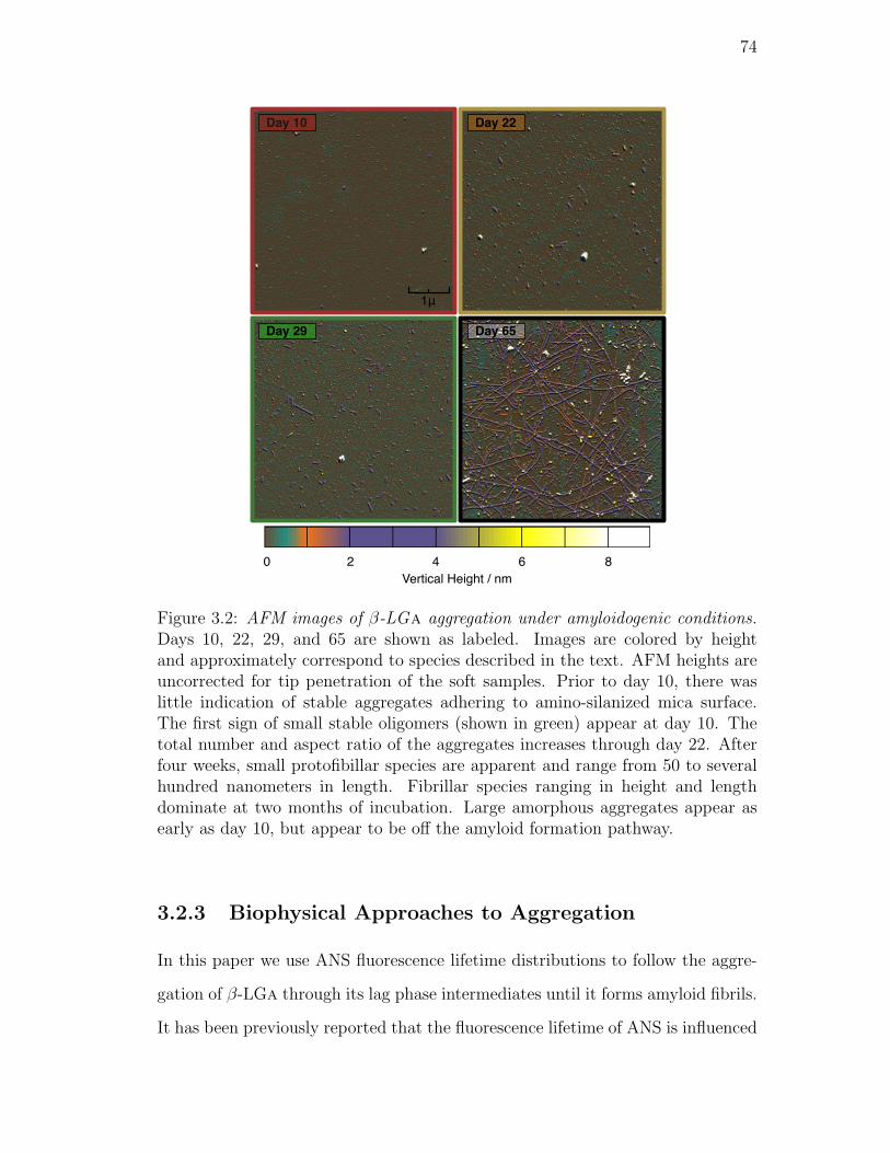
74
1μ
Vertical Height / nm0 2 4 6 8
Day 10 Day 22
Day 29 Day 65
Figure 3.2: AFM images of β-LGa aggregation under amyloidogenic conditions.Days 10, 22, 29, and 65 are shown as labeled. Images are colored by heightand approximately correspond to species described in the text. AFM heights areuncorrected for tip penetration of the soft samples. Prior to day 10, there waslittle indication of stable aggregates adhering to amino-silanized mica surface.The first sign of small stable oligomers (shown in green) appear at day 10. Thetotal number and aspect ratio of the aggregates increases through day 22. Afterfour weeks, small protofibillar species are apparent and range from 50 to severalhundred nanometers in length. Fibrillar species ranging in height and lengthdominate at two months of incubation. Large amorphous aggregates appear asearly as day 10, but appear to be off the amyloid formation pathway.
3.2.3 Biophysical Approaches to Aggregation
In this paper we use ANS fluorescence lifetime distributions to follow the aggre-
gation of β-LGa through its lag phase intermediates until it forms amyloid fibrils.
It has been previously reported that the fluorescence lifetime of ANS is influenced

75
by the polarity of its binding environment, specific interactions with amino acid
side chains, and the relative orientation and mobility of the anilino group.[59]
ANS binds to hydrophobic regions of proteins[60], and has been extensively used
to probe the presence of the molten globule state and assembly of partially struc-
tured proteins.[40, 61, 13] ANS has been observed to have different fluorescence
intensity properties when bound to different types of protein aggregates.[62] β-
LGa binds ANS in several ways,[58] including through the calyx that results in
a sequestered ANS with a very long lifetime (see Fig. 3.1). ANS probes both
the presence and integrity of this calyx as well as the overall exposure of hy-
drophobic groups in β-LGa. The calyx is of particular interest because it is the
majority of the hydrophobic core of β-LGa. Disruption of this core is required
for an aggregate to fulfill the geometric constraints of the cross-β structure of an
amyloid fibril. We use our globally regularized interior point gradient (GIPG)
fitting procedure that fits all the data simultaneously to resolve the contributions
of different ANS binding sites to the fluorescence lifetime decay.[63]
We expect aggregation to be driven, in part, by hydrophobic forces. Therefore
the parts of the protein that can bind ANS should be structurally changed by
aggregation. The ability to detect the presence of an intact calyx by virtue of
ANS binding allows determination of the involvement of, and structural changes
in, the protein hydrophobic core during amyloidogenic incubation. If the aggrega-
tion process is hydrophobically driven then we expect the aggregate to sequester
hydrophobic residues changing the structure of the calyx. Alternatively if hy-
drophobicity the key driving force for conversion to the cross-β structure, then
the large changes in the calyx should occur at that point in the incubation. In
either case the sensitivity of ANS to its binding environment should be reflected
in its fluorescence lifetime distribution.
We confirm early stages of aggregation using dynamic light scattering (DLS).
DLS has been used extensively to characterize protein aggregation and the growth
76
of amyloid.[64, 65] We explicitly evaluate the evolution of the particle size distri-
bution using the GIPG fitting procedure.[63]
We assay for the presence of amyloid using Thioflavin T (ThT) luminescence.
When bound to amyloid, ThT exhibits a new absorption band at 450 nm that has
been attributed to ThT binding to the cross-β structure.[66, 67, 68, 69, 13, 70]
The spectroscopic properties of ThT in amyloid are consistent with behavior that
has been attributed to ThT dimer formation.[71, 72, 73] The lifetime of such a
dimer will depend on its environment and geometry and some contribution of the
luminescence may arise from non-amyloid binding modes.[74] We exploit this to
detect the presence of various amyloid-like structures using a ThT luminescence
lifetime assay. The different lifetime distribution contributions and their evolution
is determined using the GIPG procedure.
We determine the morphology of the aggregates using AFM imaging. Imaging
techniques such as AFM have provided an invaluable way to determine gross mor-
phologies of amyloid protofibrils (single-stranded) and fibrils (multi-stranded).[23,
25, 26, 75]
3.3 Results
3.3.1 AFM shows sequential growth of aggregates
Fig. 3.2 shows AFM images taken on several different days of the incubation. The
images are false-colored by height to emphasize the contrast between different
classes of particles. AFM images taken from days 0 to 9 of the incubation did not
show significant signs of aggregation. The protein deposited as a uniform coating
on the functionalized mica surface (brown background in Fig. 3.2). Starting from
day 10 of the incubation, we began to see small round aggregates (green dots in
Fig. 3.2) that grew in size and number through day 22 (orange dots in Fig. 3.2).
After day 22 the number and length of oblong protofibrils increased (purple bars
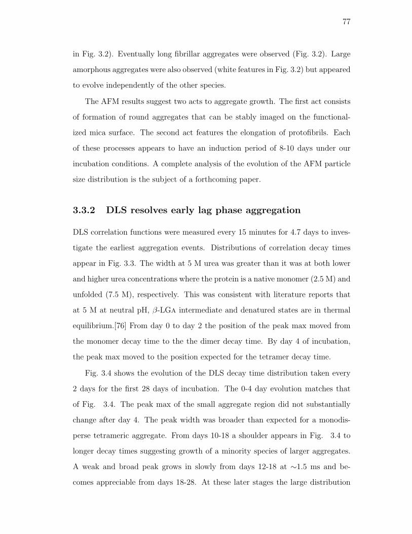
77
in Fig. 3.2). Eventually long fibrillar aggregates were observed (Fig. 3.2). Large
amorphous aggregates were also observed (white features in Fig. 3.2) but appeared
to evolve independently of the other species.
The AFM results suggest two acts to aggregate growth. The first act consists
of formation of round aggregates that can be stably imaged on the functional-
ized mica surface. The second act features the elongation of protofibrils. Each
of these processes appears to have an induction period of 8-10 days under our
incubation conditions. A complete analysis of the evolution of the AFM particle
size distribution is the subject of a forthcoming paper.
3.3.2 DLS resolves early lag phase aggregation
DLS correlation functions were measured every 15 minutes for 4.7 days to inves-
tigate the earliest aggregation events. Distributions of correlation decay times
appear in Fig. 3.3. The width at 5 M urea was greater than it was at both lower
and higher urea concentrations where the protein is a native monomer (2.5 M) and
unfolded (7.5 M), respectively. This was consistent with literature reports that
at 5 M at neutral pH, β-LGa intermediate and denatured states are in thermal
equilibrium.[76] From day 0 to day 2 the position of the peak max moved from
the monomer decay time to the the dimer decay time. By day 4 of incubation,
the peak max moved to the position expected for the tetramer decay time.
Fig. 3.4 shows the evolution of the DLS decay time distribution taken every
2 days for the first 28 days of incubation. The 0-4 day evolution matches that
of Fig. 3.4. The peak max of the small aggregate region did not substantially
change after day 4. The peak width was broader than expected for a monodis-
perse tetrameric aggregate. From days 10-18 a shoulder appears in Fig. 3.4 to
longer decay times suggesting growth of a minority species of larger aggregates.
A weak and broad peak grows in slowly from days 12-18 at ∼1.5 ms and be-
comes appreciable from days 18-28. At these later stages the large distribution
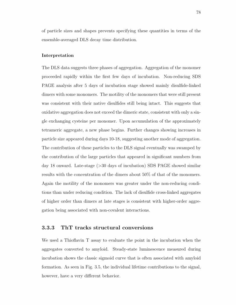
78
of particle sizes and shapes prevents specifying these quantities in terms of the
ensemble-averaged DLS decay time distribution.
Interpretation
The DLS data suggests three phases of aggregation. Aggregation of the monomer
proceeded rapidly within the first few days of incubation. Non-reducing SDS
PAGE analysis after 5 days of incubation stage showed mainly disulfide-linked
dimers with some monomers. The motility of the monomers that were still present
was consistent with their native disulfides still being intact. This suggests that
oxidative aggregation does not exceed the dimeric state, consistent with only a sin-
gle exchanging cysteine per monomer. Upon accumulation of the approximately
tetrameric aggregate, a new phase begins. Further changes showing increases in
particle size appeared during days 10-18, suggesting another mode of aggregation.
The contribution of these particles to the DLS signal eventually was swamped by
the contribution of the large particles that appeared in significant numbers from
day 18 onward. Late-stage (>30 days of incubation) SDS PAGE showed similar
results with the concentration of the dimers about 50% of that of the monomers.
Again the motility of the monomers was greater under the non-reducing condi-
tions than under reducing condition. The lack of disulfide cross-linked aggregates
of higher order than dimers at late stages is consistent with higher-order aggre-
gation being associated with non-covalent interactions.
3.3.3 ThT tracks structural conversions
We used a Thioflavin T assay to evaluate the point in the incubation when the
aggregates converted to amyloid. Steady-state luminescence measured during
incubation shows the classic sigmoid curve that is often associated with amyloid
formation. As seen in Fig. 3.5, the individual lifetime contributions to the signal,
however, have a very different behavior.
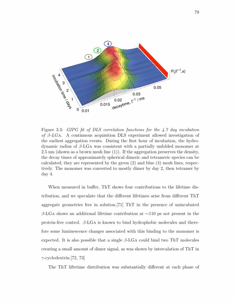
79
incu
batio
n tim
e / d
ays
decaytime, Γ-1 / m
s0.03
0.05
0.02
0.01
0.015
1
2
4
1
2
3
4
0
PI(Γ-1,x)
Figure 3.3: GIPG fit of DLS correlation functions for the 4.7 day incubationof β-LGa. A continuous acquisition DLS experiment allowed investigation ofthe earliest aggregation events. During the first hour of incubation, the hydro-dynamic radius of β-LGa was consistent with a partially unfolded monomer at2.5 nm (shown as a brown mesh line (1)). If the aggregation preserves the density,the decay times of approximately spherical dimeric and tetrameric species can becalculated; they are represented by the green (2) and blue (4) mesh lines, respec-tively. The monomer was converted to mostly dimer by day 2, then tetramer byday 4.
When measured in buffer, ThT shows four contributions to the lifetime dis-
tribution, and we speculate that the different lifetimes arise from different ThT
aggregate geometries free in solution.[71] ThT in the presence of unincubated
β-LGa shows an additional lifetime contribution at ∼110 ps not present in the
protein-free control. β-LGa is known to bind hydrophobic molecules and there-
fore some luminescence changes associated with this binding to the monomer is
expected. It is also possible that a single β-LGa could bind two ThT molecules
creating a small amount of dimer signal, as was shown by intercalation of ThT in
γ-cyclodextrin.[72, 73]
The ThT liftetime distribution was substantially different at each phase of
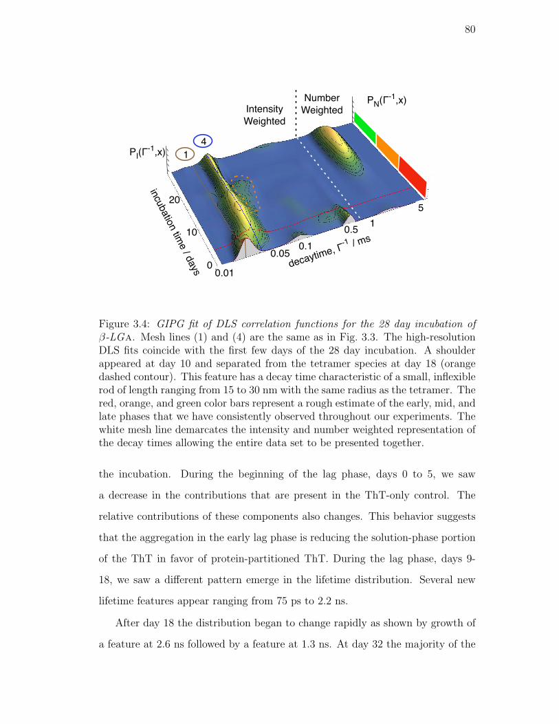
80
Number
WeightedIntensity
Weighted
incu
batio
n tim
e / d
ays decaytime, Γ
-1 / ms
PN(Γ-1,x)
0.01
0.1
0.51
5
PI(Γ-1,x) 1
4
0.05
10
20
0
Figure 3.4: GIPG fit of DLS correlation functions for the 28 day incubation ofβ-LGa. Mesh lines (1) and (4) are the same as in Fig. 3.3. The high-resolutionDLS fits coincide with the first few days of the 28 day incubation. A shoulderappeared at day 10 and separated from the tetramer species at day 18 (orangedashed contour). This feature has a decay time characteristic of a small, inflexiblerod of length ranging from 15 to 30 nm with the same radius as the tetramer. Thered, orange, and green color bars represent a rough estimate of the early, mid, andlate phases that we have consistently observed throughout our experiments. Thewhite mesh line demarcates the intensity and number weighted representation ofthe decay times allowing the entire data set to be presented together.
the incubation. During the beginning of the lag phase, days 0 to 5, we saw
a decrease in the contributions that are present in the ThT-only control. The
relative contributions of these components also changes. This behavior suggests
that the aggregation in the early lag phase is reducing the solution-phase portion
of the ThT in favor of protein-partitioned ThT. During the lag phase, days 9-
18, we saw a different pattern emerge in the lifetime distribution. Several new
lifetime features appear ranging from 75 ps to 2.2 ns.
After day 18 the distribution began to change rapidly as shown by growth of
a feature at 2.6 ns followed by a feature at 1.3 ns. At day 32 the majority of the
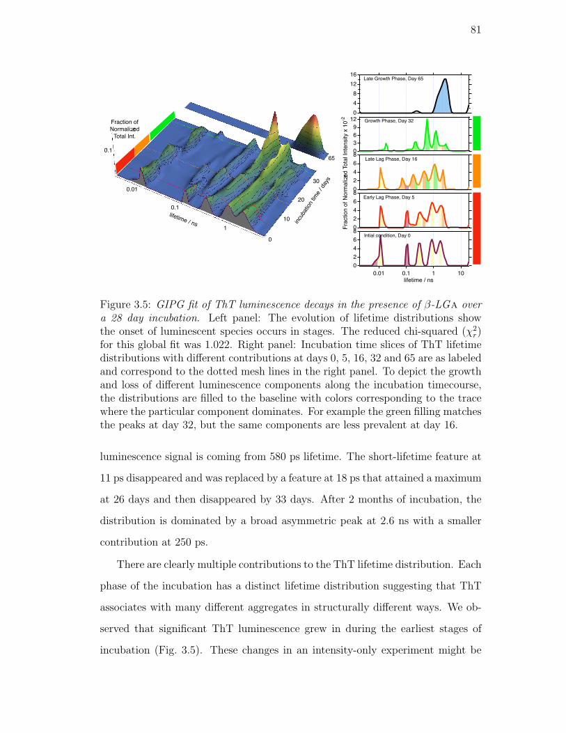
81
incubation time / days
lifetime / ns
0.01
0.1
1
10
65
30
0
8
6
4
2
0
0.01 0.1 1 10
lifetime
8
6
4
2
0
8
6
4
2
0
12
9
6
3
0
16
12
8
4
0
Fraction of
Normalized
Total Int.
10
20
Fraction of Normalized Total Intensity x 10-2
0.1
lifetime / ns
Intial condition, Day 0
Early Lag Phase, Day 5
Late Lag Phase, Day 16
Growth Phase, Day 32
Late Growth Phase, Day 65
Figure 3.5: GIPG fit of ThT luminescence decays in the presence of β-LGa overa 28 day incubation. Left panel: The evolution of lifetime distributions showthe onset of luminescent species occurs in stages. The reduced chi-squared (χ2
r)for this global fit was 1.022. Right panel: Incubation time slices of ThT lifetimedistributions with different contributions at days 0, 5, 16, 32 and 65 are as labeledand correspond to the dotted mesh lines in the right panel. To depict the growthand loss of different luminescence components along the incubation timecourse,the distributions are filled to the baseline with colors corresponding to the tracewhere the particular component dominates. For example the green filling matchesthe peaks at day 32, but the same components are less prevalent at day 16.
luminescence signal is coming from 580 ps lifetime. The short-lifetime feature at
11 ps disappeared and was replaced by a feature at 18 ps that attained a maximum
at 26 days and then disappeared by 33 days. After 2 months of incubation, the
distribution is dominated by a broad asymmetric peak at 2.6 ns with a smaller
contribution at 250 ps.
There are clearly multiple contributions to the ThT lifetime distribution. Each
phase of the incubation has a distinct lifetime distribution suggesting that ThT
associates with many different aggregates in structurally different ways. We ob-
served that significant ThT luminescence grew in during the earliest stages of
incubation (Fig. 3.5). These changes in an intensity-only experiment might be

82
interpreted as a baseline shift. The association of monomers into a disordered
aggregate may provide ThT with the opportunity to form dimers that show lu-
minescence similar to amyloid, however the lack of a regular geometry results
in a different lifetime. Particularly striking is the difference between the 580 ps
contribution that seems to appear in association with protofibrils and the 2.6 ns
contribution that appears in the late-stage aggregation where mature amyloid fib-
rils are present. The signal from ThT usually associated with histological staining
is probably most closely related to the distribution from the 65 day sample. The
ThT signal changes that contribute to the classic sigmoidal intensity kinetic trace
are most likely due to other binding modes and luminescence lifetimes. This sug-
gests that the pro-amyloid ThT luminescence has a structural sensitivity that is
reflected in its luminescence lifetime distribution. ThT assays based only upon
intensity could be misleading since there are several contributions to the lumines-
cence that are potentially changing during incubation. The contributions from
the different species cannot be resolved from intensity alone.
3.3.4 ANS reports changes in hydrophobic regions and
calyx loss.
The fluorescence lifetime of ANS was measured during 28 days of amyloidogenic
incubation. We used GIPG as a model-free approach to determine the evolution
of the ANS fluorescence assay lifetime distribution. We observed several peaks
in the distribution that change systematically with incubation time and labeled
them (a) though (i) for clarity as shown in Fig. 3.6. Some of these peaks change
during the first several days of the incubation. Others grow in at the late stages
of the incubation. The evolution of individual peaks can be associated with the
changes in the availability of specific binding environments on β-LGa in its various
aggregation states. To directly evaluate the evolution of the contributions from
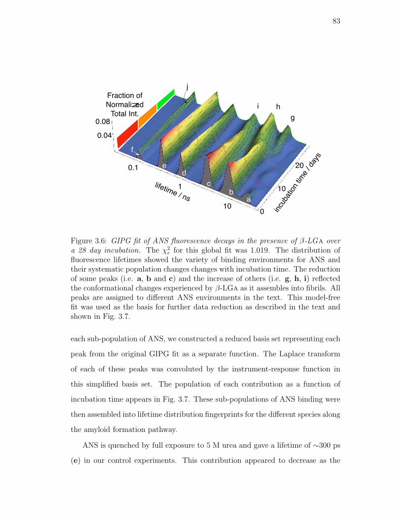
83
incubation time / days
0.1
1
20
10
10
0.04
Fraction of
Normalized
Total Int.
0
lifetime / ns ab
c
de
f
g
hi
j
0.08
Figure 3.6: GIPG fit of ANS fluorescence decays in the presence of β-LGa overa 28 day incubation. The χ2
r for this global fit was 1.019. The distribution offluorescence lifetimes showed the variety of binding environments for ANS andtheir systematic population changes changes with incubation time. The reductionof some peaks (i.e. a, b and c) and the increase of others (i.e. g, h, i) reflectedthe conformational changes experienced by β-LGa as it assembles into fibrils. Allpeaks are assigned to different ANS environments in the text. This model-freefit was used as the basis for further data reduction as described in the text andshown in Fig. 3.7.
each sub-population of ANS, we constructed a reduced basis set representing each
peak from the original GIPG fit as a separate function. The Laplace transform
of each of these peaks was convoluted by the instrument-response function in
this simplified basis set. The population of each contribution as a function of
incubation time appears in Fig. 3.7. These sub-populations of ANS binding were
then assembled into lifetime distribution fingerprints for the different species along
the amyloid formation pathway.
ANS is quenched by full exposure to 5 M urea and gave a lifetime of ∼300 ps
(e) in our control experiments. This contribution appeared to decrease as the

84
80
60
40
20
0
2520151050
incubation time / days
40
30
20
10
0
Fraction of Time Zero Intensity x 10-3
6
4
2
0
400
300
200
100
0
2.7 ns
2.1 ns
7.9 ns
4.9 ns
18 ns
11 ns
89 ps 70 ps
300 ps 790 ps
(c)
(i)
(b)
(h)
(a)
(g)
(f)
(e) (j)
(d)
Figure 3.7: Sub-populations of ANS binding to β-LGa over a 28 day incubationusing GIPG with reduced basis set. The χ2
r for this global fit was 1.020. In thetop three panels, the red squares represent the decreasing lifetimes and the bluetriangles represent increasing lifetimes corresponding to the sub-populations inFig. 3.6. The species lifetime evolutions are associated with a change in the ANSenvironment in the calyx or surface sites. The bottom panel shows the trends ofthe short lifetime components. The lettering (a) though (i) matches the peaks inFig. 3.6. The red and orange dotted vertical lines mark the lifetime componentsat days 8 and 16 which were combined with those at days 0 and 28 to generatethe characteristic “fingerprints” of the ANS-bound protein species and shown inFig. 3.8.
incubation progressed. This suggested an increase in the partitioning of ANS
with the protein as compared to the solution and was consistent with an overall
increase in the availability of hydrophobic binding sites as the incubation proceeds.
The model-free GIPG fit in Fig. 3.6 shows an 89 ps feature (f), which was
85
also present in the ANS lifetime distribution from 1 to 6 M urea in our control
experiments, but only when β-LGa was also present. This feature appeared to
increase in population from days 0 to 14 then decrease from days 16 to 28. The
89 ps contribution overlapped with a broad lifetime contribution at 70 ps (j) that
grew in starting at day 18. The increase in this contribution appeared to com-
pensate for the loss of the 89 ps contribution. These lifetimes were significantly
shorter than that of the free ANS, suggesting a quenching interaction with an
amino acid side chain.
The monomeric signal included contributions from peaks at 18.2 ns (a), 7.9 ns
(b), and 2.7 ns (c). The peak at 18.2 ns was close to the unquenched lifetime of
∼19 ns predicted by an evaluation of the oscillator strength using the Strickler-
Berg equation.[77] This suggested that ANS was sequestered from any quenchers
and was protected from water, consistent with an intact calyx. This feature
decreased throughout the incubation. ANS can induce structure in proteins and
the presence of folded β-LGa under these conditions may be a result of this effect.
No other lifetime feature in the distribution appears to compensate for the loss
of the 18.2 ns feature.
The peak at 7.9 ns (b) also suggested protection from water, though to a lesser
degree. This was consistent with a partially denatured calyx. The 7.9 ns feature
decreased dramatically in the first 8 days, leveling off until day 18, whereupon
it continued to decrease. The changes in the 7.9 ns contribution appeared to
be mostly compensated by changes in a feature at 4.9 ns (h). The highly anti-
correlated behavior of the 7.9 ns and 4.9 ns components suggested that the 4.9 ns
feature was from ANS bound to β-LGa that had its 7.9 ns calyx site disrupted
by aggregation.
The peak at 2.7 ns (c) has been previously attributed to β-LGa surface
binding.[76] Based on our ANS docking studies we found that the mouth of the
calyx is a more likely assignment for this feature. The 2.7 ns feature decreased

86
rapidly at first, its evolution slowing after 8 days, and accelerating again during
the late stages of incubation. The 2.7 ns feature population changes were partly
compensated by changes in the 2.1 ns feature (i). Again, this close relationship
leads us to conclude that the mouth of the calyx is being disrupted during the
process that exchanges the population of the 2.7 ns and 2.1 ns features.
Overall, the changes in the ANS lifetime distributions occurring after day 20
were more dramatic. One of these was an 11 ns feature (g) that appeared to
grow in at the late stages of incubation. The long lifetime suggests that ANS
was mostly isolated from water. We attribute it to sequestration of ANS in the
cross-β structure of amyloid protofibrils.
Not all of the lifetime features changed over the incubation timecourse. The
feature at 790 ps (d) was present throughout the incubation with only small
changes in intensity. Therefore the 790 ps site should be a structure that was not
disrupted in the aggregation process. This lifetime was consistent with surface
binding, which should be present at all points of the incubation. The 790 ps
lifetime appeared to shift slightly at different points in the fits in Fig. 3.6. These
shifts were too small to reliably resolve multiple lifetime contributions to this
feature.
Any particular ANS lifetime peak can, in principle, contribute to several dif-
ferent aggregates. The binding location as reflected in the lifetime is sensitive
to the local environment, but not the specific aggregation state. Nevertheless,
the relative contribution of each binding site to a particular aggregate should be
in some fixed proportion that depends on the structure of the β-LGa monomers
in it. During amyloidogenic incubation we see three main phases in the kinetic
evolution of the ANS lifetime distribution that are corroborated by other experi-
ments. We seek to separate contributions of at least four species with qualitatively
different aggregation states.
We assumed that the contributions of different species could be expressed as
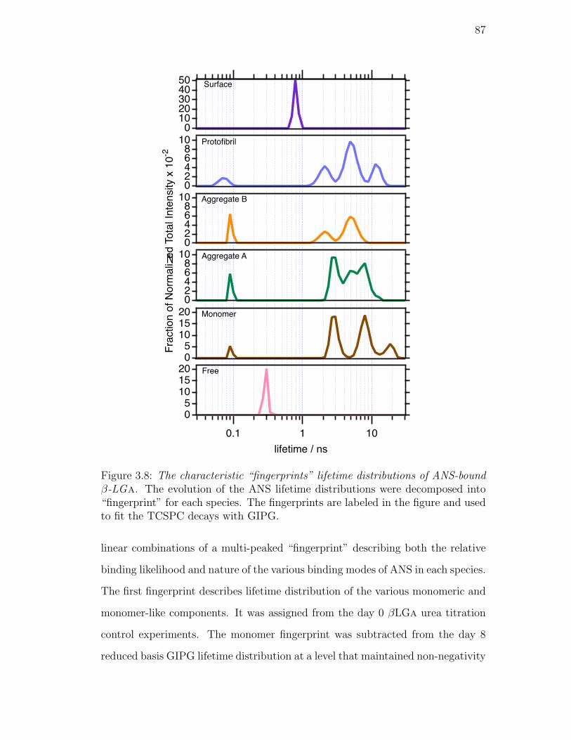
87
20
15
10
5
0
0.1 1 10
lifetime / ns
20
15
10
5
0
1086420
1086420
x10-2
1086420
50403020100
Surface
Protofibril
Aggregate B
Aggregate A
Monomer
Free
Fraction of Normalized Total Intensity x 10-2
Figure 3.8: The characteristic “fingerprints” lifetime distributions of ANS-boundβ-LGa. The evolution of the ANS lifetime distributions were decomposed into“fingerprint” for each species. The fingerprints are labeled in the figure and usedto fit the TCSPC decays with GIPG.
linear combinations of a multi-peaked “fingerprint” describing both the relative
binding likelihood and nature of the various binding modes of ANS in each species.
The first fingerprint describes lifetime distribution of the various monomeric and
monomer-like components. It was assigned from the day 0 βLGa urea titration
control experiments. The monomer fingerprint was subtracted from the day 8
reduced basis GIPG lifetime distribution at a level that maintained non-negativity
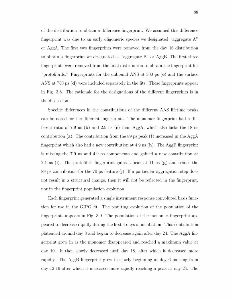
88
of the distribution to obtain a difference fingerprint. We assumed this difference
fingerprint was due to an early oligomeric species we designated “aggregate A”
or AggA. The first two fingerprints were removed from the day 16 distribution
to obtain a fingerprint we designated as “aggregate B” or AggB. The first three
fingerprints were removed from the final distribution to obtain the fingerprint for
“protofibrils.” Fingerprints for the unbound ANS at 300 ps (e) and the surface
ANS at 750 ps (d) were included separately in the fits. These fingerprints appear
in Fig. 3.8. The rationale for the designations of the different fingerprints is in
the discussion.
Specific differences in the contributions of the different ANS lifetime peaks
can be noted for the different fingerprints. The monomer fingerprint had a dif-
ferent ratio of 7.9 ns (b) and 2.9 ns (c) than AggA, which also lacks the 18 ns
contribution (a). The contribution from the 89 ps peak (f) increased in the AggA
fingerprint which also had a new contribution at 4.9 ns (h). The AggB fingerprint
is missing the 7.9 ns and 4.9 ns components and gained a new contribution at
2.1 ns (i). The protofibril fingerprint gains a peak at 11 ns (g) and trades the
89 ps contribution for the 70 ps feature (j). If a particular aggregation step does
not result in a structural change, then it will not be reflected in the fingerprint,
nor in the fingerprint population evolution.
Each fingerprint generated a single instrument response convoluted basis func-
tion for use in the GIPG fit. The resulting evolution of the population of the
fingerprints appears in Fig. 3.9. The population of the monomer fingerprint ap-
peared to decrease rapidly during the first 4 days of incubation. This contribution
plateaued around day 8 and began to decrease again after day 24. The AggA fin-
gerprint grew in as the monomer disappeared and reached a maximum value at
day 10. It then slowly decreased until day 18, after which it decreased more
rapidly. The AggB fingerprint grew in slowly beginning at day 6 pausing from
day 12-16 after which it increased more rapidly reaching a peak at day 24. The
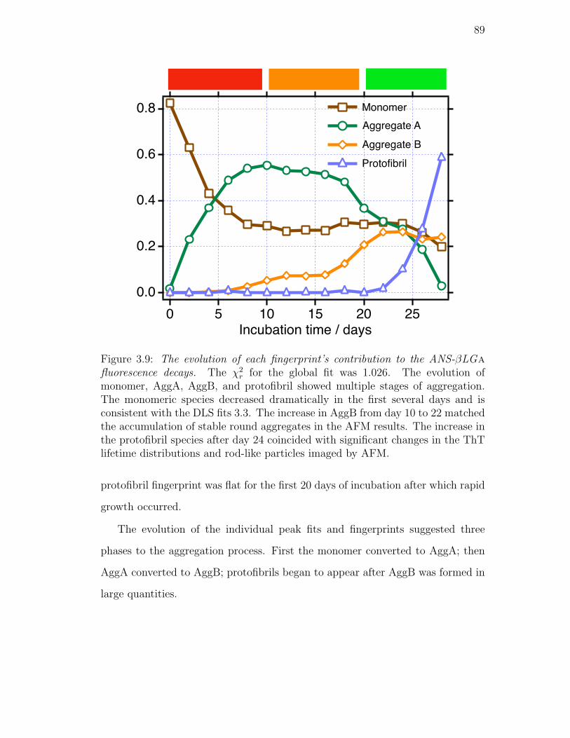
89
0.8
0.6
0.4
0.2
0.0
2520151050
Incubation timeIncubation time / days
Monomer
Aggregate A
Protofibril
Aggregate B
Figure 3.9: The evolution of each fingerprint’s contribution to the ANS-βLGafluorescence decays. The χ2
r for the global fit was 1.026. The evolution ofmonomer, AggA, AggB, and protofibril showed multiple stages of aggregation.The monomeric species decreased dramatically in the first several days and isconsistent with the DLS fits 3.3. The increase in AggB from day 10 to 22 matchedthe accumulation of stable round aggregates in the AFM results. The increase inthe protofibril species after day 24 coincided with significant changes in the ThTlifetime distributions and rod-like particles imaged by AFM.
protofibril fingerprint was flat for the first 20 days of incubation after which rapid
growth occurred.
The evolution of the individual peak fits and fingerprints suggested three
phases to the aggregation process. First the monomer converted to AggA; then
AggA converted to AggB; protofibrils began to appear after AggB was formed in
large quantities.
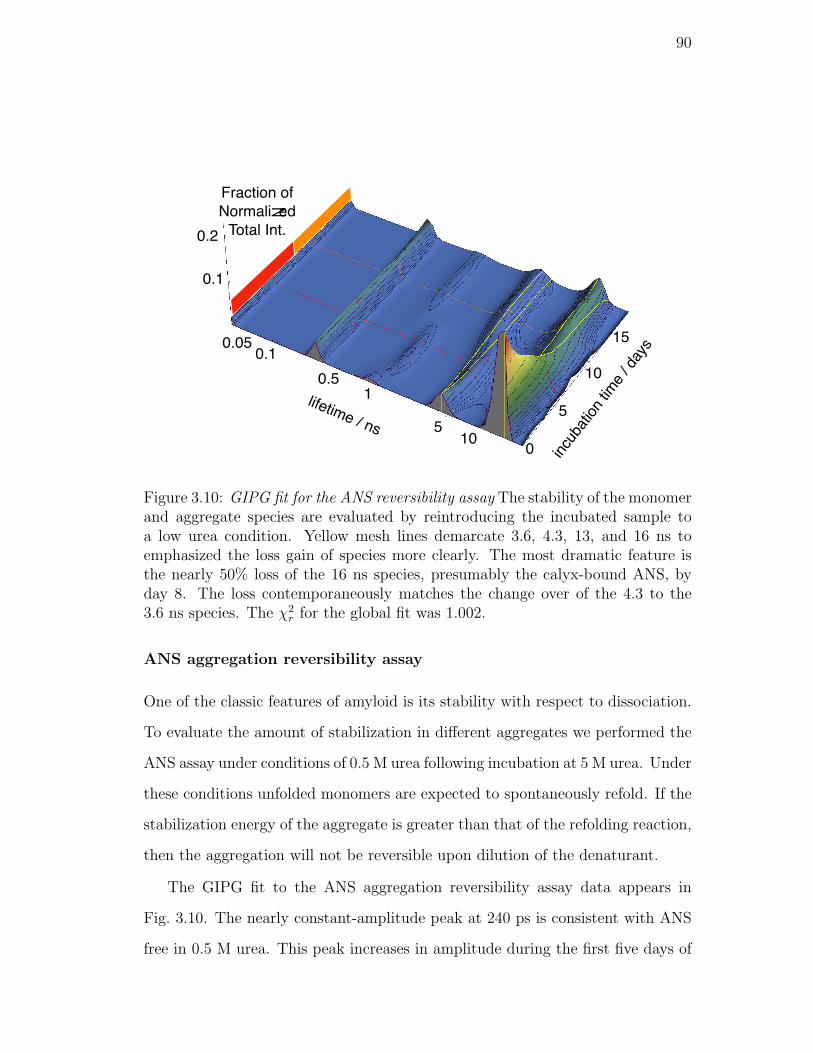
90
incubation time / days
0.10.05
0.5
lifetime / ns
1
510
0.2
0
5
10
15
0.1
Fraction of
Normalized
Total Int.
Figure 3.10: GIPG fit for the ANS reversibility assay The stability of the monomerand aggregate species are evaluated by reintroducing the incubated sample toa low urea condition. Yellow mesh lines demarcate 3.6, 4.3, 13, and 16 ns toemphasized the loss gain of species more clearly. The most dramatic feature isthe nearly 50% loss of the 16 ns species, presumably the calyx-bound ANS, byday 8. The loss contemporaneously matches the change over of the 4.3 to the3.6 ns species. The χ2
r for the global fit was 1.002.
ANS aggregation reversibility assay
One of the classic features of amyloid is its stability with respect to dissociation.
To evaluate the amount of stabilization in different aggregates we performed the
ANS assay under conditions of 0.5 M urea following incubation at 5 M urea. Under
these conditions unfolded monomers are expected to spontaneously refold. If the
stabilization energy of the aggregate is greater than that of the refolding reaction,
then the aggregation will not be reversible upon dilution of the denaturant.
The GIPG fit to the ANS aggregation reversibility assay data appears in
Fig. 3.10. The nearly constant-amplitude peak at 240 ps is consistent with ANS
free in 0.5 M urea. This peak increases in amplitude during the first five days of

91
incubation and then decreases slightly until day 9 and then increases again with
the increase accelerating after day 14.
At day 0, the peak associated with surface binding at 830 ps did not appear at
its 0.5 M control experiment position suggesting that the association at this site
was somewhat irreversible. From days 2 to 8 the peak was shifted to its reversible
position at 1.1 ns and from days 10-18 it shifted to 790 ps. This result may
indicate that there was a kinetic competition between refolding of the surface
site, perhaps at the α-helix, and binding of ANS. If this is the case, it would
suggest that during days 2-8 the binding site was protected from ANS until after
refolding had occurred. The overall amplitude of this peak did not change much,
consistent with the results of the standard ANS assay.
The peak at 16 ns was consistent with binding to the calyx and decreased
rapidly from days 0 to 4 and continued to decrease more slowly from days 6 to
12. This peak was replaced by a feature at 14 ns that appeared around day 1,
increased until day 14 and decreased thereafter. Around day 18 the peak shifted
to 13 ns. The rapid decrease in the availability of the calyx suggests that the
aggregates in the early stages prevented the binding of ANS to the calyx. The
shifts in lifetime suggest that though some structure resembling a calyx can reform
as late as day 18, the population of these proteins is substantially reduced and
that they cannot reform the full calyx that is possible before aggregation has
occurred.
We attributed the peak at 4.3 ns to the outer calyx binding site. This lifetime
was shorter than the 5.4 ns we determined from the 0.5 M control measurement.
This suggests a degree of irreversibility even at day 0 in this binding site. This
feature decreased from days 0 to 4, leveled out from days 5 to 8, and then decayed
away from days 8 to 12. This feature was replaced by a peak at 3.6 ns that
increased until day 12 after which it remained steady from 14 to 18 days. Overall
the qualitative behavior of this feature was similar to the feature at 16 ns.

92
There were essentially three manifestations of irreversibility represented in
this data. The first was the ability of the protein to regain the same ANS binding
sites after dilution from 5 M to 0.5 M urea as determined by the lifetime distri-
bution. The dilution was performed in the presence of ANS. If the ANS binds
to the site in question prior to refolding, then it could lock the protein into a
misfolded conformation at the binding site. The result is a lifetime that more
closely resembles the 5 M urea control experiment conditions than the 0.5 M urea
conditions. The second type of irreversibility was the loss of a particular binding
site as aggregation progresses. This suggests that the aggregate disrupts or blocks
access to the site in question and that the site cannot be reformed by dilution
of the denaturant. The third type of irreversibility was the replacement of one
site with another. This is similar to the second type of irreversibility, except that
the structural change has resulted in a new local environment for the binding of
ANS.
These three types of irreversibility suggest that there are two main stages to
the incubation over the range of 0 to 18 days that appear to transition at 8 to
10 days. The changes that were reflected in the irreversibility suggested that
one of the key elements distinguishing the different aggregation steps was the
reversibility of the interactions between monomers in the different aggregates.
3.4 Discussion
3.4.1 Conformationally lability prior to incubation
Our results suggest that βLGa was conformationally labile under the amyloido-
genic incubation conditions. The Thioflavin T assay showed little change in signal
over the protein-free control except for an additional peak at 110 ps. The ANS
assay showed several lifetime components and a substantial contribution from
intact-calyx-binding of ANS suggesting that ANS may be stabilizing the folded
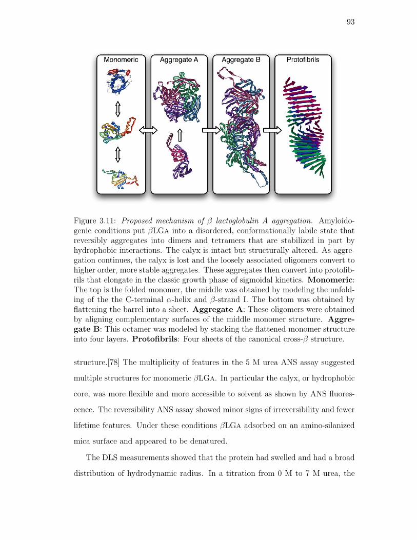
93
Figure 3.11: Proposed mechanism of β lactoglobulin A aggregation. Amyloido-genic conditions put βLGa into a disordered, conformationally labile state thatreversibly aggregates into dimers and tetramers that are stabilized in part byhydrophobic interactions. The calyx is intact but structurally altered. As aggre-gation continues, the calyx is lost and the loosely associated oligomers convert tohigher order, more stable aggregates. These aggregates then convert into protofib-rils that elongate in the classic growth phase of sigmoidal kinetics. Monomeric:The top is the folded monomer, the middle was obtained by modeling the unfold-ing of the the C-terminal α-helix and β-strand I. The bottom was obtained byflattening the barrel into a sheet. Aggregate A: These oligomers were obtainedby aligning complementary surfaces of the middle monomer structure. Aggre-gate B: This octamer was modeled by stacking the flattened monomer structureinto four layers. Protofibrils: Four sheets of the canonical cross-β structure.
structure.[78] The multiplicity of features in the 5 M urea ANS assay suggested
multiple structures for monomeric βLGa. In particular the calyx, or hydrophobic
core, was more flexible and more accessible to solvent as shown by ANS fluores-
cence. The reversibility ANS assay showed minor signs of irreversibility and fewer
lifetime features. Under these conditions βLGa adsorbed on an amino-silanized
mica surface and appeared to be denatured.
The DLS measurements showed that the protein had swelled and had a broad
distribution of hydrodynamic radius. In a titration from 0 M to 7 M urea, the

94
width of the DLS RH distribution was broadest at 5 M urea. That the width of the
distribution is resolvable, implied the exchange time within that distribution was
longer than the characteristic diffusion time of ∼20 µs. Amyloid formation from
βLGa has been observed to be fastest at 5 M urea.[13] The day 0 DLS results
showed that the conditions giving the maximum rate of amyloidogenesis were
coincident with those that created the maximum variance in the hydrodynamic
radius of βLGa.
Overall we can conclude that there are multiple monomeric structures that
are exchanging in the sample under these conditions. The partially folded in-
termediate appeared to be the aggregation-prone state. The ability to exchange
between multiple conformations may be a crucial feature in determining aggrega-
tion propensity. To use free energy landscape language, the folding funnel flattens,
allowing access to disordered states of increased RH and core solvation.
3.4.2 Early lag phase aggregation was more reversible
The DLS assay showed that aggregation occurs in the first few days of incuba-
tion with average particle sizes passing through a dimeric stage to a steady state
with an average size consistent with tetramers. In the AFM assay, the aggre-
gates could be imaged on a clean mica surface, but on a more strongly adsorbing
amino-silainzed mica surface the aggregates were disrupted and denatured on the
surface. The ANS 5 M urea assay revealed a decreased ability of ANS to bind to
the calyx. The irreversibility assay showed changes predominantly in the calyx
binding site. The fingerprint analysis of the ANS 5 M urea assay suggested that a
new species was growing in, with a small contribution from another species. We
call these species AggA and AggB, respectively. The differences in fingerprints
suggested changes in the nature and relative populations of different binding sites
and therefore a change in the tertiary structure of the monomers upon aggrega-
tion. However, the ThT assay only showed small changes in lifetime distribution

95
implying that this structural change was not to the cross-β structure associated
with amyloid.
The stabilization energy of AggA was less than the electrostatic interaction
with the amino-silanized mica surface. However, AggA was not disrupted by
dilution into more native-like conditions suggesting that the AggA stabilization
energy was between the folding energy and the surface adsorption energy. The
interaction between monomers in AggA most likely involved some change or dis-
ruption of the calyx that allowed solvent access. Some parts of the structural
changes that occurred upon forming AggA were still reversible at this stage. This
suggested that the structure of βLGa in AggA more closely resembled the free
monomer than does AggB. AggA appeared to be limited in total size. Contin-
ued growth most likely required disruption of the remaining free-monomer-like
structure. AggA in Fig. 3.11 was modeled with swapping of structural elements.
This type of interaction is possible because of the inherent self-complimentary
nature of folded proteins. These interactions are also likely to sterically limit the
maximum size of aggregates that could be so assembled.
3.4.3 Late lag phase aggregation loses calyx
During the late lag phase small aggregates were possible to image on the amino-
silanized mica surface. In the DLS assay, the appearance of a wing on the distri-
bution to larger RH and the growth of a new feature at large RH suggest aggregate
growth resuming during this stage. The ThT assay shows a new pattern in the
lifetime distribution. The ANS fingerprint analysis showed that AggB begins
to get appreciable population while AggA decreases in population, suggesting a
conversion from AggA to AggB. The ANS irreversibility assay showed that AggB
had new binding sites for ANS. This suggested that the structural conversion was
inside of the aggregate rather than a newly formed aggregate.

96
Conversion to AggB appeared to be required for growth to continue. The sta-
bility of AggB with respect to dissociation on the amino-silanized surface implied
that it was more stable than AggA. AggB was larger, on average, than AggA. The
monomer structure changed from AggA to AggB as reflected in the changes in the
ANS assay binding sites. AggB was also structurally different than AggA in terms
of the monomer-monomer interactions as suggested by the ANS reversibility as-
say. The changes in AggB structure allowed ThT-ThT interactions that were not
possible in AggA. The ThT assay implied that some elements of the AggB struc-
ture might be similar to those in amyloid fibril. However, no fibrils or protofibrils
were observed at this stage. The ThT lifetime contributions of fibrillar species
were different than those of AggB. Conversion to AggB could be misinterpreted
as amyloid formation if only changes in ThT intensity were measured.
3.4.4 Protofibrils appeared after day 20
During the growth phase the light scattering intensity increased enormously and
the amount of large aggregate increased. AFM images showed the appearance of
protofibrils followed by elongation of protofibrils and finally fibril assembly into
long fibrils of varying length and diameter. The ANS assay showed dramatic
growth in the protofibril fingerprint, a decrease in the AggA fingerprint, and a
steady state for the AggB fingerprint. At very long incubation times very little
ANS binding was observed to mature fibrils suggesting the presence of accessi-
ble hydrophobic regions on the protofibrils that disappeared upon formation of
mature fibrils. We speculate that these hydrophobic locations are involved in
the lateral association of protofibrils into fibrils. The ThT assay showed a new
lifetime distribution pattern that continued to grow until at least day 34. We
associated this pattern with amyloid protofibrils since the distribution was still
very different than that observed from mature fibrils. Only some of the protofibril
features were present in the ThT assay taken after 2 months of incubation where
97
mature fibrils were present. A large ThT lifetime contribution was present in
the mature fibril data that was not present at any other stage. The structure of
protofibrils must be different at the ThT binding level from that of fibrils.
3.4.5 Overall mechanism
The native β-strands in β-LGa are not in the right orientation to attain the cross-
β geometry. It appears likely that an interaction analogous to domain swapping
or opening of the β-sheet “sandwich” would be required for β-LGa to associate
into the cross-β geometry. Based on the observed morphology of amyloid fibrils
and the size of β-LGa, it would require approximately 2-3 β-LGa monomers, or
4-6 flattened monomers, to form the transverse structure of a 4-5 nm diameter
fibril. A fibril of ∼45 nm in length would contain ∼32 β-LGa monomers and have
a total molecular weight of 590 kDa. A fully formed amyloid fibril of 10 nm x
200 nm would contain ∼700 β-LGa monomers and have a total molecular weight
of 12.9 MDa.
Our results suggest that there are two parts to the lag phase of βLGa amy-
loid formation. The sequence of events is similar to some recent kinetic analyses
of amyloid nucleation.[22] We monitored the role of the hydrophobic core using
the signature lifetime of ANS in the calyx. We showed how fluorescence lifetime
fingerprints can be used to extract the contribution of multiple species during
incubation. We identified two intermediates in the lag phase that are distin-
guishable by their relative stability, size, and binding of ThT and ANS. ANS is
sensitive to the rigidity and polarity of binding locations, while ThT is sensitive
to the relative geometry of its ThT binding sites. Based on this information, we
must conclude that significant rearrangement of structure must occur between
AggA and AggB. The standard interpretation of this change would be that AggB
represents the conversion to the amyloid nucleus. However, ThT gave different
signals when bound to AggA, AggB, and protofibrils. Moreover, the onset of

98
rapid growth of protofibrils does not occur until many days after the appearance
of AggB. Therefore we must conclude that AggB is distinct in structure from
both AggA and protofibrils. The presence of multiple aggregated species in a
serial mechanism suggests that homogenous nucleation may not be a universal
description of amyloid formation kinetics.
The initial aggregation into AggA and subsequent aggregation into AggB must
have some driving force associated with them. Two simple models, colloidal ag-
gregation and polymer phase stability, can be invoked to frame the initial ag-
gregation. The inherent hydrophobicity of the polypeptide chain can lead to an
aggregated phase of protein being more stable.[16] The driving force in this case is
the increased number of favorable protein-protein and water-water contacts and
a decreased number of protein-water contacts. Colloidal aggregation is similar
except that it attributes the driving force to the partitioning of amino acids with
unfavorable protein-water contact energies into a region of higher protein-protein
contacts while amino acids with favorable protein-water contact energies are par-
titioned to the surface of the aggregate. This partitioning puts an additional
geometric constraint on the aggregation process that is not present in the phase
stability picture.
Given the large number of charged amino acids on βLGa we favor the col-
loidal aggregation picture, however our data only indirectly addresses this issue.
Colloidal association in AggA and then AggB could reduce the barrier to the
conformational change to cross-β required to form amyloid. Colloidal associa-
tion is required because the monomer cannot rearrange without sacrificing a pro-
hibitively large number of hydrophobic interactions. If the protein has a strong
hydrophobic core, then the hydrophobic effect is too strong to disrupt. If the
protein is completely unfolded the possible hydrophobic gains are too weak to
overcome the translational entropy lost to aggregation.
There is a connection to protein folding in this analysis. Proteins below a
99
certain size typically cannot stably fold. This can be attributed to there not be-
ing a large enough number of favorable interactions to meet the thermodynamic
conditions of cooperativity. By associating into colloidal or phase-separated ag-
gregates, the protein increases its effective molecular weight and potential number
of favorable interactions to the point where the fold of amyloid is accessible. This
colloidal or phase-separated promotion of conformational rearrangement may ex-
plain the ability of surfactants to promote amyloid formation.
Amyloidogenic conditions have been identified for many non-disease-related
proteins. This leads to the hypothesis that aggregation of proteins leading to amy-
loid fibril formation is a generic feature of polypeptides.[79, 7] If the hypothesis
that amyloidogenesis is a generic possibility for proteins is valid, then we should
think about amyloid as a particular state of protein in the polypeptide phase
diagram. The driving forces for phase separation into amyloid should depend on
the relative contributions of hydrogen bonding in the cross-β structure and the
arrangement of hydrophobic groups. There is evidence that the polypeptide is
hydrophobic from a polymer physics point of view, i.e. that polymer-polymer
contacts are more energetically favorable than polymer-water contacts.[80, 81]
This would suggest that the environmental and sequence determinants for amy-
loid propensity are more based on the lowering of the barrier to formation of the
amyloid phase than on stability of the amyloid phase itself. In other words the
effects are principally kinetic rather than thermodynamic. In particular in this
study we propose that the initial aggregation to AggA allows a larger hydrophobic
core to be formed in AggB. This allows the cross-β structure to be obtained in
the protofibril. The initial bistability of the monomer allows formation of AggA.
AggA allows a lower-barrier pathway to formation of AggB which is large enough
to rearrange into the more stable cross-β structure without a prohibitively large
activation barrier. This allows the spontaneous formation of amyloid protofibrils
to occur even when barriers to formation of the cross-β structure directly from

100
the monomer or even AggA is energetically prohibitive.
3.5 Materials and Methods
3.5.1 Materials
Lyophilized β-LGa, thioflavin T, urea, APTES, sodium phosphate dibasic and
mono-basic were purchased from Sigma. Fluorescence grade 8-anilino-1-naphthalenesulfonic
acid ammonium salt (ANS) was purchased from Fluka.
A 10 mM sodium phosphate, pH 7.0 stock buffer solution was prepared with
HPLC grade water. This buffer was used to prepare a second stock buffer con-
taining 7.5 M urea. Both stock buffers were filtered through a 0.22 µm PES
filter and stored at 4C. For DLS measurements, extra care was taken to mini-
mize scattering from dust contaminants by filtering stock buffer solutions with a
pre-washed, 0.020 µm syringe filter (Whatman). The 0 M urea stock phosphate
buffer was used to prepare a 138 µM stock protein solution of β-LGa and stored
at 4C. The protein stock solution was checked by UV absorption every few days
to ensure its stability.
3.5.2 β-LGa incubations
We incubated β-LGa under conditions previously reported to show maximum
amyloidogenicity[13] and aliquoted samples for time-resolved ANS and ThT lu-
minescence, DLS, and AFM experiments.
For time-resolved luminescence and DLS measurements, 1.5 mL of protein
sample for incubation was prepared every other day for 28 days and used for ANS
assay along with the long-term DLS experiments. For ThT and ANS reversibility
assay, samples were prepared every day for 34 days and 18 days, respectively.
Each incubation sample was prepared by combining a 500 µL aliquot of the stock
101
protein solution to 1000 µL of the 7.5 M urea stock solution in a polypropylene
eppendorf tube resulting in a final protein concentration of 46 µM and a final
urea concentration of 5 M. The sample was capped, sealed with Parafilm, and
placed in an incubator at 37C. At the conclusion of the incubation, all samples
were breached and each was parsed for contemporaneous experimentation.
To investigate the earliest aggregation with DLS, a sample of 46 µM β-LGa in
5 M urea, 10 mM sodium phosphate at pH 7.0 was prepared from the stock solu-
tions above. The sample filled the cuvette to approximately 90% capacity in order
to reduce the sample head space. Dynamic light scattering was measured while
simultaneously incubated at 37C in a Peltier sample chamber (instrumentation
discussed below).
For the AFM measurements, lyophilized β-LGa was reconstituted and dia-
lyzed against pre-filtered (0.22 µm) 100 mM phosphate buffer, pH 7.0. Prefiltered
concentrated urea buffer was added resulting in a final sample condition for in-
cubation of 50 µM protein in 5 M urea, 13.7 mM sodium phosphate at pH 7.0.
The sample was incubated in a Parafilm-sealed 1.5 mL Eppendorf tube at 37C
over 65 days. The sample was inverted once each day that AFM was measured
and 20 µL was aliquoted for the AFM image.
3.5.3 Time-resolved luminescence
Time-resolved luminescence was measured by time-correlated single photon count-
ing (TCSPC). Experimental set up has been previously described[82] with the
exception that the Spectra Physics Tsunami Ti:Sapphire laser was operated in
femtosecond mode. All samples were analyzed at 37C in a Quantum North-West
TLC150 Peltier controller sample chamber (Spokane, WA).
For the ThT assay, a stock 5 µM ThT solution was prepared from the 0 M
urea stock buffer. 50 µL of an incubated timepoint was aliquoted into 450 µL of
ThT solution in a reduced volume cuvette and allowed to stand for 15 minutes
102
at 37C. The excitation laser was tuned to 450 nm and the luminescence was
observed at 482 nm. The time zero intensity ranged between 30,000 and 60,000
photons. A 50 ns collection window was used. Instrument response functions
typically had a full-width at half-maximum (fwhm) of approximately 90 ps.
A 80 µM ANS stock solution was prepared in a 0 M urea stock buffer for the
ANS assay. 500 µL of an incubated timepoint was combined with 10 µL of the
ANS stock solution and allowed to stand for 15 minutes at 37C.
For the ANS reversibility assay, a 1 µM ANS stock solution was prepared
in a 0 M urea stock buffer. 50 µL of an incubated timepoint was combined
with 450 µL of the ANS stock solution and allowed to stand for 15 minutes at
37C. Excitation beam was tuned to 390 nm and the fluorescence emission was
observed at 485 nm over a 100 and 82 ns collection windows for the ANS and
ANS reversibility assays, respectively. A typical transient’s time zero intensity was
4,000 for the ANS reversibility assay, whereas 18,000 photons was common for the
ANS assay. Instrument response functions typically had a fwhm of approximately
100 ps.
We expect the population of the luminescent species to be piecewise contin-
uous with respect to incubation time, making this system a prime candidate for
global data analysis by the GIPG method.[63, 82]. ThT luminescence lifetime dis-
tributions were fit on an 80-point grid, logarithmically spaced in lifetime, ranging
from 0.002 to 20 ns. Both types of ANS assays were fit on there own 58-point log-
arithmically spaced between ranging from 0.03 to 30 ns. A baseline and scattering
term was included in the fits. To compensate for potential incident laser intensity
fluctuations across incubation time, all TCSPC transients were normalized by the
total time-zero photon population. This is accomplished by summing the param-
eters from a non-negative least squares fit [83, 63] The GIPG fits were considered
statistically indistinguishable from the local fits by calculating the probability-to-
reject [63, 84] to be less than 10−4 for all fits. ThT, ANS and ANS reversibility
103
assays GIPG fits used 8 × 10⁵, 1 × 10⁶, 1.5 × 10⁶ iterations, respectively. The
GIPG step scaling term referred to as λ, was set to 0.9.
3.5.4 Dynamic light scattering
Fluctuations of scattered light intensity were measured using a homodyne tech-
nique. At a particular incubation time, x, the intensity correlation function
g2(t, x), was measured by a modified Nicomp Model 380 Particle Size Analyzer
from Particle Sizing Systems. Scattered light from the incident laser, λ=532 nm,
was collected orthogonally, θ=90. The system employs a linearly-scaled 64-
channel digital autocorrelator. For experiments completed in this paper, the
native autocorrelator was bypassed by an ALV-6010 Multi-Tau autocorrelator
(ALV-GmbH, Langen, Germany) for the maximum possible statistical accuracy
across several orders of magnitude in decay time.[85]
Round borosilicate glass cuvettes (Kimble Glass) were used for all DLS mea-
surements. In order to minimize dust contamination, each cuvette was rinsed with
Millipore water. Cuvettes were placed in a micro-centrifuge, inverted (open-side
face-down), then spun dry and stored face down. After sample was quickly and
carefully added to the cuvette, it was covered with transparent tape to keep it
dust-free, then wrapped in Parafilm for an additional seal.
For the 28 day DLS study, 250 µL of incubated sample was placed in a clean,
dry cuvette. Twenty correlation functions were measured sequentially for 30
seconds apiece for each incubated sample. The cuvette chamber was held at
a constant temperature of 37C. For the continuous acquisition incubation, the
same sample was analyzed every 15 minutes for 5 minutes at 37C for 4.7 days.
The distribution of decay rates, f(Γ, x), for particular incubation time point,
x is related to the field correlation function, g1(t, x), by
g1(t, x) =
∫ ∞0
e−Γtf(Γ, x) dΓ, (3.1)
104
where f(Γ, x) can be solved for by the inverse Laplace transform. In most cases,
the intensity and field correlation functions can be related via the Siegert relation,
such that√g2(t, x)− 1 ∝ g1(t, x).[85]
GIPG was originally demonstrated by globally fitting TCSPC transients, but
it can be also employed to globally fit many types of spectroscopic data that
require an inverse Laplace transform, such as in Eq. 3.1, as long as there is
piecewise continuity in the experimental domain, x. One difference is that the
intensity correlation functions do not require instrument-response convolution of
the basis set. Another difference is that the standard deviations for the data were
calculated in real time by the ALV-6010 correlator using a noise model.
DLS data was globally fit on a 50-point grid of logarithmically-spaced decay
times, Γ−1, ranging from 0.001 to 65 ms. A baseline term was included. The
total number of correlation functions used in the short-term DLS fit was reduced
340 to 34 by averaging every ten correlation functions into a single trace and
propagating the error accordingly. The probability-to-reject the GIPG solution
for both data sets was less than 10−4.
In DLS, a particle’s decaytime is related to the translational diffusion constant
though the scattering vector, q, such that D = Γ/q2, where q = 4nπ/λ sin(θ/2),
where n is the refractive index. The diffusion constant can then be converted
to Stokes-hydrodynamic radius (RH) using the Stokes-Einstein relation, RH =
(kbT )/(6πη0D), assuming a spherical shape. For these experiments, T is the
temperature, η0 is the viscosity of the buffer, and kb is the Boltzmann constant.
The characteristic density of the partially unfolded monomer determined from
assignment of a urea titration DLS experiment at 5.0 M was used to scale the
oligomer sizes.

105
3.5.5 Atomic force microscopy
To obtain better adhesion of protein aggregates to a mica surface, a chemical sur-
face modification was implemented. 20 uL of 0.1 (V/V) APTES (Aminopropyl-
triethoxysilane) was applied evenly on freshly cleaved 9.9 mm diameter mica disk.
After 10 minutes unreacted APTES was rinsed away with 15 mL 0.2 µM filtered
deionized water. The surface was blown dry with high purity compressed nitrogen
gas. Incubated sample was applied evenly on freshly prepared surface for 10 min-
utes. Unbound species were rinsed away with Millipore water. The sample was
again dried with nitrogen gas before being imaged with a MultiMode Scanning
Probe Microscope (Digital Instruments) with a TESP tip in tapping mode.
3.6 Acknowledgments
This work was supported by a grant from the National Institutes of Health
#R01GM071684. JTG was supported by a Graduate Assistantship in Areas of
National Need grant to the Department of Chemistry and Chemical Biology. We
thank Ben Strangfeld for assisting with the dynamic light scattering experiments,
Troy Messina for IMPACT minimizations, and Richard Ebright for the use the
AFM.
106
References
[1] J. D. Sipe, A. S. Cohen, Review: History of the amyloid fibril, Journal ofStructural Biology 130 (2/3) (2000) 88–98.
[2] D. M. Walsh, D. M. Hartley, D. J. Selkoe, The many faces of aβ: Struc-tures and activity, Current Medicinal Chemistry: Immunology, Endocrine &Metabolic Agents 3 (4) (2003) 277–291.
[3] R. Wetzel, Ideas of order for amyloid fibril structure, Structure 10 (8) (2002)1031–1036.
[4] B. Solomon, Towards alzheimer’s disease vaccination, Mini-Rev. Med. Chem.2 (1) (2002) 85–92.
[5] M. D. Kirkitadze, G. Bitan, D. B. Teplow, Paradigm shifts in alzheimer’s dis-ease and other neurodegenerative disorders: the emerging role of oligomericassemblies, J. Neurosci. Res. 69 (5) (2002) 567–577.
[6] J. Hardy, D. J. Selkoe, The amyloid hypothesis of Alzheimer’s disease:progress and problems on the road to therapeutics, Science 297 (5580) (2002)353–356.
[7] F. Chiti, C. Dobson, Protein misfolding, functional amyloid, and humandisease, Annual Reviews Biochemistry 75 (2006) 333–366.
[8] D. B. Teplow, Structural and kinetic features of amyloid β-protein fibrillo-genesis, Amyloid 5 (2) (1998) 121–142.
[9] J.-C. Rochet, J. Lansbury, Peter T., Amyloid fibrillogenesis: themes andvariations, Curr. Opin. Struct. Biol. 10 (1) (2000) 60–68.
[10] R. M. Murphy, M. M. Pallitto, Probing the kinetics of β-amyloid self-association, Journal of Structural Biology 130 (2/3) (2000) 109–122.
[11] E. Zerovnik, Amyloid-fibril formation. proposed mechanisms and relevanceto conformational disease, European Journal of Biochemistry 269 (14) (2002)3362–3371.
[12] L. Nielsen, R. Khurana, A. Coats, S. Frokjaer, J. Brange, S. Vyas, Effect ofenvironmental factors on the kinetics of insulin fibril formation: Elucidationof the molecular mechanism, Biochemistry 40 (2001) 6036–6046.
107
[13] D. Hamada, C. M. Dobson, A kinetic study of β-lactoglobulin amyloid fibrilformation promoted by urea, Protein Sci. 11 (10) (2002) 2417–2426.
[14] C.-C. Lee, A. Nayak, A. Sethuraman, G. Belfort, G. J. McRae, A three-stagekinetic model of amyloid fibrillation, Biophysical Journal Volume 92 (2007)3448–3458.
[15] A. Lomakin, D. B. Teplow, D. A. Kirschner, G. B. Benedek, Kinetic theoryof fibrillogenesis of amyloid β-protein, Proc. Natl . Acad. Sci . USA 94 (1997)7942–7947.
[16] R. V. Pappu, X. Wang, A. Vitalis, S. L. Crick, A polymer physics perspectiveon driving forces and mechanisms for protein aggregation, Arch. Biochem.Biophys. 469 (2008) 132–141.
[17] M. M. Pallitto, R. M. Murphy, A mathematical model of the kinetics of β-amyloid fibril growth from the denatured state, Biophys. J. 81 (2001) 1805–1822.
[18] R. Kayed, E. Head, J. L. Thompson, T. M. McIntire, S. C. Milton, C. W.Cotman, C. G. Glabe, Common structure of soluble amyloid oligomers im-plies common mechanism of pathogenesis, Science 300 (2003) 486–489.
[19] M. D. Kane, W. J. Lipinski, M. J. Callahan, F. Bian, R. A. Durham, R. D.Schwarz, A. E. Roher, L. C. Walker, Evidence for seeding of β-amyloidby intracerebral infusion of alzheimer brain extracts in β-amyloid precursorprotein-transgenic mice, The Journal of Neuroscience 20 (2000) 3606–3611.
[20] J. D. Harper, P. T. Lansbury, Jr., Models of amyloid seeding in alzheimer’sdisease and scrapie: mechanistic truths and physiological consequences of thetime-dependent solubility of amyloid proteins., Annual Review Biochemistry66 (1997) 385–407.
[21] J. Stohr, N. Weinmann, H. Wille, T. Kaimann, L. Nagel-Steger, E. Birk-mann, G. Panza, S. B. Prusiner, M. Eigen, D. Riesner, Mechanisms of prionprotein assembly into amyloid, Proc. Natl. Acad. Sci. U. S. A. 105 (2008)2409 –2414.
[22] J. M. Andrews, C. J. Roberts, A lumry-eyring nucleated polymerizationmodel of protein aggregation kinetics: 1. aggregation with pre-equilibratedunfolding, The Journal Physical Chemistry B 111 (2007) 7897–7913.
[23] C. Goldsbury, J. Kistler, U. Aebi, T. Arvinte, G. J. S. Cooper, Watchingamyloid fibrils grow by time-lapse atomic force microscopy, J. Mol. Biol.285 (1) (1999) 33–39.
[24] M. Stolz, D. Stoffler, U. Aebi, C. Goldsbury, Monitoring biomolecular inter-actions by time-lapse atomic force microscopy, Journal of Structural Biology131 (3) (2000) 171–180.
108
[25] W. S. Gosal, A. H. Clark, P. D. A. Pudney, S. B. Ross-Murphy, Novel amyloidfibrillar networks derived from a globular protein: β-lactoglobulin, Langmuir18 (19) (2002) 7174–7181.
[26] A. Parbhu, H. Lin, J. Thimm, R. Lal, Imaging real-time aggregation ofamyloid β protein (1-42) by atomic force microscopy, Peptides 23 (7) (2002)1265–1270.
[27] Y. Kusumoto, A. Lomakin, D. B. Teplow, G. B. Benedek, Temperaturedependence of amyloid β-protein fibrillization, Proc. Natl. Acad. Sci. U. S.A. 95 (21) (1998) 12277–12282.
[28] F. Bergasa-Caceres, H. A. Rabitz, Two-state folding kinetics of small proteinsin the sequential collapse model: Dependence of the folding rate on contactorder and temperature, J. Phys. Chem. B 107 (46) (2003) 12874–12877.
[29] S. B. Prusiner, Novel proteinaceous infectious particles cause scrapie, Science216 (4542) (1982) 136–144.
[30] J. S. Griffith, Self-replication and scrapie, Nature 215 (105) (1967) 1043–1044.
[31] D. Schenk, Opinion: Amyloid-β immunotherapy for alzheimer’s disease: theend of the beginning, Nat. Rev. Neurosci. 3 (10) (2002) 824–828.
[32] K. S. Satheeshkumar, R. Jayakumar, Conformational polymorphism of theamyloidogenic peptide homologous to residues 113-127 of the prion protein,Biophys. J. 85 (1) (2003) 473–483.
[33] M. Bouchard, J. Zurdo, E. J. Nettleton, C. M. Dobson, C. V. Robinson,Formation of insulin amyloid fibrils followed by ftir simultaneously with cdand electron microscopy, Protein Sci. 9 (2000) 1960–1967.
[34] J. Lansbury, Peter T., P. R. Costa, J. M. Griffiths, E. J. Simon, M. Auger,K. J. Halverson, D. A. Kocisko, Z. S. Hendsch, T. T. Ashburn, et al., Struc-tural model for the β-amyloid fibril based on interstrand alignment of anantiparallel-sheet comprising a c-terminal peptide, Nature Structural Biol-ogy 2 (11) (1995) 990–998.
[35] F. Chiti, P. Webster, N. Taddei, A. Clark, M. Stefani, G. Ramponi, C. M.Dobson, Designing conditions for in vitro formation of amyloid protofila-ments and fibrils, Proc. Natl. Acad. Sci. U. S. A. 96 (7) (1999) 3590–3594.
[36] H. Abe, H. Nakanishi, Novel observation of a circular dichroism band origi-nating from amyloid fibril, Anal. Sci. 19 (1) (2003) 171–173.
[37] R. Carrotta, R. Bauer, R. Waninge, C. Rischel, Conformational character-ization of oligomeric intermediates and aggregates in β-lactoglobulin heataggregation, Protein Sci. 10 (7) (2001) 1312–1318.
109
[38] V. Baskakov Ilia, G. Legname, A. Baldwin Michael, B. Prusiner Stanley,E. Cohen Fred, Pathway complexity of prion protein assembly into amyloid,J. Biol. Chem. 277 (24) (2002) 21140–21148.
[39] A. Quintas, M. J. Saraiva, R. M. Brito, The tetrameric protein transthyretindissociates to a non-native monomer in solution. a novel model for amyloido-genesis, J. Biol. Chem. 274 (46) (1999) 32943–32949.
[40] J. Safar, P. P. Roller, D. C. Gajdusek, J. Gibbs, C. J., Scrapie amyloid (prion)protein has the conformational characteristics of an aggregated molten glob-ule folding intermediate, Biochemistry 33 (27) (1994) 8375–8383.
[41] S. Srisailam, S. Kumar Thallampuranam Krishnaswamy, D. Rajalingam,M. Kathir Karuppanan, H.-S. Sheu, F.-J. Jan, P.-C. Chao, C. Yu, Amyloid-like fibril formation in an all β-barrel protein. partially structured intermedi-ate state(s) is a precursor for fibril formation, J. Biol. Chem. 278 (20) (2003)17701–17709.
[42] P. M. Gorman, A. Chakrabartty, Alzheimer β-amyloid peptides: structuresof amyloid fibrils and alternate aggregation products, Biopolymers 60 (5)(2001) 381–394.
[43] T. H. J. Huang, D.-S. Yang, P. E. Fraser, A. Chakrabartty, Alternate ag-gregation pathways of the alzheimer β-amyloid peptide. an in vitro model ofpreamyloid, J. Biol. Chem. 275 (46) (2000) 36436–36440.
[44] S. Uhrinova, M. H. Smith, G. B. Jameson, D. Uhrin, L. Sawyer, P. N.Barlow, Structural changes accompanying ph-induced dissociation of the β-lactoglobulin dimer, Biochemistry 39 (13) (2000) 3565–3574.
[45] L. Sawyer, G. Kontopidis, The core lipocalin, bovine β-lactoglobulin,Biochim. Biophys. Acta 1482 (2000) 136–148.
[46] L. M. C. Sagis, C. Veerman, E. Van der Linden, Mesoscopic properties ofsemiflexible amyloid fibrils, Langmuir 20 (3) (2004) 924–927.
[47] M. Buck, Trifluoroethanol and colleagues: cosolvents come of age. recentstudies with peptides and proteins, Quarterly Reviews of Biophysics 31 (3)(1998) 297–355.
[48] G. Chikenji, M. Kikuchi, What is the role of non-native intermediates ofβ-lactoglobulin in protein folding?, Proc. Natl. Acad. Sci. U. S. A. 97 (26)(2000) 14273–14277.
[49] V. Forge, M. Hoshino, K. Kuwata, M. Arai, K. Kuwajima, C. A. Batt,Y. Goto, Is folding of β-lactoglobulin non-hierarchic? intermediate withnative-like β-sheet and non-native α-helix, J. Mol. Biol. 296 (4) (2000) 1039–1051.
110
[50] D. Hamada, Y. Goto, The equilibrium intermediate of β-lactoglobulin withnon-native α-helical structure, J. Mol. Biol. 269 (4) (1997) 479–487.
[51] D. Hamada, S.-i. Segawa, Y. Goto, Non-native α-helical intermediate in therefolding of β-lactoglobulin, a predominantly β-sheet protein, Nature Struc-tural Biology 3 (10) (1996) 868–873.
[52] K. Kuwata, M. Hoshino, S. Era, C. A. Batt, Y. Goto, α → β transitionof β-lactoglobulin as evidenced by heteronuclear nmr, J. Mol. Biol. 283 (4)(1998) 731–739.
[53] F. Bergasa-Caceres, H. A. Rabitz, Sequential collapse folding pathway ofβ-lactoglobulin: Parallel pathways and non-native secondary structure, J.Phys. Chem. B 107 (v 15) (2003) 3606–3612.
[54] K. Kuwajima, H. Yamaya, S. Sugai, The burst-phase intermediate in therefolding of β-lactoglobulin studied by stopped-flow circular dichroism andabsorption spectroscopy, J. Mol. Biol. 264 (4) (1996) 806–822.
[55] K. Kuwata, R. Shastry, H. Cheng, M. Hoshino, C. A. Batt, Y. Goto,H. Roder, Structural and kinetic characterization of early folding events inβ-lactoglobulin, Nature Structural Biology 8 (2) (2001) 151–155.
[56] N. K. Kella, J. E. Kinsella, Structural stability of β-lactoglobulin in the pres-ence of kosmotropic salts. a kinetic and thermodynamic study., InternationalJournal of Peptide and Protein Research , pp. 32 (1988) 396–405.
[57] L. K. Creamer, Effect of sodium dodecyl sulfate and palmitic acid on theequilibrium unfolding of bovine β-lactoglobulin?, Biochemistry 34 (1995)7170–7176.
[58] L. D’Alfonso, M. Collini, G. Baldini, Trehalose influence on β-lactoglobulinstability and hydration by time resolved fluorescence, European Journal ofBiochemistry 270 (11) (2003) 2497–2504.
[59] W. Kirk, E. Kurian, W. Wessels, Photophysics of ans v. decay modes of ansin proteins: The ifabp-ans complex, Biophys. Chem. 125 (2007) 50–58.
[60] O. K. Gasymov, A. R. Abduragimov, B. J. Glasgow, Characterization offluorescence of ans-tear lipocalin complex: Evidence for multiple-bindingmodes, Photochem. Photobiol. 83 (2007) 1405–1414.
[61] R. Khurana, J. R. Gillespie, A. Talapatra, L. J. Minert, C. Ionescu-Zanetti,I. Millett, A. L. Fink, Partially folded intermediates as critical precursors oflight chain amyloid fibrils and amorphous aggregates, Biochemistry 40 (12)(2001) 3525–3535.
111
[62] M. Lindgren, K. Sorgjerd, P. Hammarstromy, Detection and characterizationof aggregates, prefibrillar amyloidogenic oligomers, and protofibrils using flu-orescence spectroscopy, Biophys. J. 88 (2005) 4200–4212.
[63] J. T. Giurleo, D. S. Talaga, Global fitting without a global model: Regular-ization based on the continuity of the evolution of parameter distributions,The Journal of Chemical Physics 128 (2008) 114114–(1–18).
[64] A. Lomakin, G. B. Benedek, D. B. Teplow, Monitoring protein assemblyusing quasielastic light scattering spectroscopy, Method in Enzymology 309(1999) 429–459.
[65] A. J. Modler, K. Gast, G. Lutsch, G. Damaschun, Assembly of amyloidprotofibrils via critical oligomers-a novel pathway of amyloid formation, J.Mol. Biol. 325 (1) (2003) 135–148.
[66] F. S. Waldrop, H. Puchtler, S. N. Meloan, Fluorescent thiazole stains foramyloid without differentiation, Journal of Histotechnology 7 (3) (1984) 123–126.
[67] A. Elhaddaoui, A. Delacourte, S. Turrell, Spectroscopic study of congo redand thioflavin binding to amyloid-like proteins, J. Mol. Struct. 294 (1993)115–118.
[68] I. LeVine, Harry, Thioflavine t forms uniquely fluorescent complexes withamyloid structures of synthetic alzheimer’s disease β-amyloid peptides andinsulin in solution, Amyloid Amyloidosis 1993, Proc. Int. Symp. Amyloidosis,7th (1994) 383–385.
[69] I. LeVine, Harry, Thioflavine t interaction with amyloid β-sheet structures,Amyloid 2 (1) (1995) 1–6.
[70] T. Ban, D. Hamada, K. Hasegawa, H. Naiki, Y. Goto, Direct observation ofamyloid fibril growth monitored by thioflavin t fluorescence, J. Biol. Chem.278 (19) (2003) 16462–16465.
[71] R. Schirra, Dye aggregation in freezing aqueous solutions, Chem. Phys. Lett.119 (1985) 463–466.
[72] R. R. C. Retna Raj, γ-cyclodextrin induced intermolecular excimer formationof thioflavin t, Chem. Phys. Lett. 273 (1997) 285–290.
[73] M. Groenning, L. Olsen, M. van de Weert, J. M. Flink, S. Frokjaer, F. S.Jørgensen, Study on the binding of thioxavin t to β-sheet-rich and non-β–sheet cavities, Journal of Structural Biology 158 (2007) 358–369.
[74] W. F. Weiss, T. K. Hodgdon, E. W. Kaler, A. M. Lenhoff, C. J. Roberts,Nonnative protein polymers: Structure, morphology, and relation to nucle-ation and growth, Biophys. J. 93 (2007) 4392–4403.
112
[75] M. Gaczynska, P. A. Osmulski, Afm of biological complexes: What can welearn?, Current Opinion in Colloid Interface Science in Press.
[76] L. D’Alfonso, M. Collini, G. Baldini, Does β-lactoglobulin denaturation occurvia an intermediate state?, Biochemistry 41 (2002) 326–333.
[77] S. J. Strickler, R. A. Berg, Relationship between absorption intensity andfluorescence lifetime of molecules, The Journal of Chemical Physics 37 (1962)814–822.
[78] D. W. Miller, K. A. Dill, Ligand binding to proteins: The binding landscapemodel, Protein Sci. 6 (1997) 2166–2179.
[79] C. M. Dobson, Protein misfolding, evolution and disease, Trends Biochem.Sci. 24 (9) (1999) 329–332.
[80] S. L. Crick, M. Jayaraman, C. Frieden, R. Wetzel, R. V. Pappu, Fluorescencecorrelation spectroscopy shows that monomeric polyglutamine moleculesform collapsed structures in aqueous solutions, Proc. Natl. Acad. Sci. U.S. A. 103 (2006) 16764–16769.
[81] A. Vitalis, X. Wang, R. V. Pappu, Quantitative characterization of intrinsicdisorder in polyglutamine: Insights from analysis based on polymer theories,Biophys. J. 93 (2007) 1923–1937.
[82] T. C. Messina, H. Kim, J. T. Giurleo, D. S. Talaga, Hidden markov modelanalysis of multichromophore photobleaching, J. Phys. Chem. B 110 (2006)16366–16376.
[83] C. L. Lawson, R. J. Hanson, Solving Least Squares Problems, Prentice-Hall,Inc., 1974.
[84] S. W. Provencher, A contrained regularization method for inverting data rep-resented by linear algebraic or integral equations, Comput. Phys. Commun.27 (1982) 213–227.
[85] W. Brown (Ed.), Dynamic Light Scattering, The Method and Some Appli-cations, Oxford Science Publications, 1993.
[86] J. L. Banks, H. S. Beard, Y. Cao, A. E. Cho, W. Damm, R. Farid, A. K. Felts,T. A. Halgren, D. T. Mainz, J. R. Maple, R. Murphy, D. M. Philipp, M. P.Repasky, L. Y. Zhang, B. J. Berne, R. A. Friesner, E. Gallicchio, R. M. Levy,Integrated modeling program, applied chemical theory (impact), J. Comput.Chem. 26 (2005) 1752–1780.
113
Chapter 4
Exploring αSyn with covalently attached
fluorophores using time-resolved and single
molecule imaging spectroscopy
4.1 Summary
In recent years, time-resolved fluorescence techniques have become very useful
for elucidating a host of biophysical problems. Using conformationally sensitive
fluorescent probes allows the differentiation of local environments and the abil-
ity to infer conformational changes in the host molecule. The downside is that
multiple lifetimes acquired for a single system can be complicated to understand.
We take two approaches to solve this: global analysis of bulk data and utilizing
single molecule imaging spectroscopy. The first approach can be accomplished
by acquiring data transients while simultaneously, but smoothly, perturbing an
experimental coordinate, such as temperature, wavelength, denaturant concen-
tration, etc. It is then applicable to utilize the globally regularized interior point
gradient method to determine the lifetime components of the system without the
need to a specify a model a priori (see Chap. 2 for details). [1] In the second ap-
proach, we can avoid the ensemble averaging present in all bulk experiments by
employing single molecule lifetime imaging [2] to identify characteristic lifetimes
species-by-species.
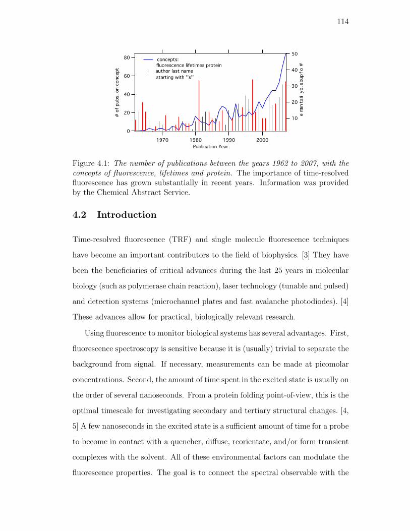
114
80
60
40
20
0
# o
f pubs.
on c
oncept
2000199019801970
Publication Year
50
40
30
20
10
# o
f pubs. b
y la
st n
am
e
concepts: fluorescence lifetimes protein
author last name
starting with ''s''
Figure 4.1: The number of publications between the years 1962 to 2007, with theconcepts of fluorescence, lifetimes and protein. The importance of time-resolvedfluorescence has grown substantially in recent years. Information was providedby the Chemical Abstract Service.
4.2 Introduction
Time-resolved fluorescence (TRF) and single molecule fluorescence techniques
have become an important contributors to the field of biophysics. [3] They have
been the beneficiaries of critical advances during the last 25 years in molecular
biology (such as polymerase chain reaction), laser technology (tunable and pulsed)
and detection systems (microchannel plates and fast avalanche photodiodes). [4]
These advances allow for practical, biologically relevant research.
Using fluorescence to monitor biological systems has several advantages. First,
fluorescence spectroscopy is sensitive because it is (usually) trivial to separate the
background from signal. If necessary, measurements can be made at picomolar
concentrations. Second, the amount of time spent in the excited state is usually on
the order of several nanoseconds. From a protein folding point-of-view, this is the
optimal timescale for investigating secondary and tertiary structural changes. [4,
5] A few nanoseconds in the excited state is a sufficient amount of time for a probe
to become in contact with a quencher, diffuse, reorientate, and/or form transient
complexes with the solvent. All of these environmental factors can modulate the
fluorescence properties. The goal is to connect the spectral observable with the

115
molecular features of the system.
In this chapter, we evaluate the fluorescence properties of three different cova-
lently attached fluorophores to α-synuclein (αSyn) using time-correlated single-
photon counting (TCSPC). αSyn is an intrinsically disordered protein (IDP) [6]
found in the brain. αSyn aggregates into highly structured pathogenic fibrils and
is implicated in Parkinson’s Disease. [7, 8]
Time-averaged, or steady-state, fluorescence measurements fall quantitatively
short of reporting on the multi-state properties of the system. [4] Only by measur-
ing fluorescence lifetimes can the separate components of the intensity signal be
ascertained. In chapter 3, we showed the power of elucidating the evolution life-
time distribution of an environmentally-sensitive, non-covalently attached probe
in order to determine aggregation states of β-lactoglobulin A. [9]
The lifetime distribution of a covalently attached fluorophore can report envi-
ronmental changes undergone by αSyn along an experimental coordinate (temper-
ature, incubation time, etc.). However, as the number of environments increases,
the lifetime analysis can become unstable. In chapter 2, we combat this issue by
applying a novel global analysis method to stabilize lifetime fitting called globally
regularized interior point gradient method (GIPG). [1]
Single molecule fluorescence imaging of aggregates with covalently attached
fluorophores can be utilized to elucidate the lifetime components on a species-by-
species basis. To differentiate between monomers, aggregates and fibrils, several
images are taken. With each pass, species photobleach. Monomers are expected
to be dim and photobleach easily in just a few image passes. Oligomers will
stepwise lose intensity as the dye is bleached. Fibrils are expected to have at
least two defining features: high intensity and several hundred nanometers long
or more. By keeping track of photobleaching steps for any aggregate, it is possible
to calculate the number of monomers per aggregate [10].
Nile Red (NR) is a solvatochromatic dye. The emission of NR is red-shifted
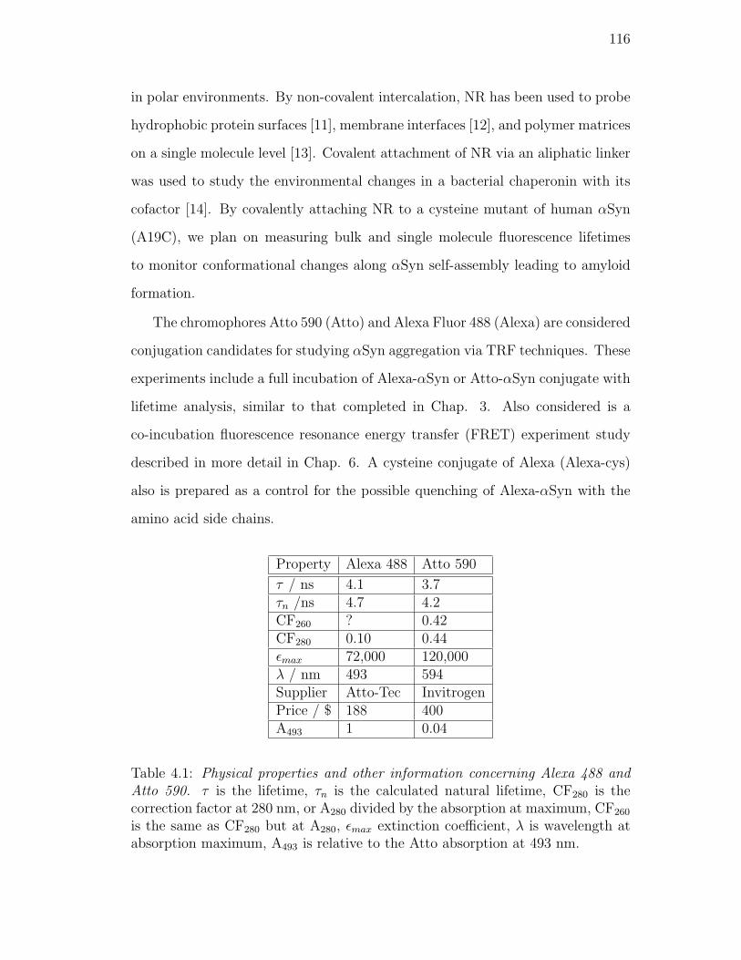
116
in polar environments. By non-covalent intercalation, NR has been used to probe
hydrophobic protein surfaces [11], membrane interfaces [12], and polymer matrices
on a single molecule level [13]. Covalent attachment of NR via an aliphatic linker
was used to study the environmental changes in a bacterial chaperonin with its
cofactor [14]. By covalently attaching NR to a cysteine mutant of human αSyn
(A19C), we plan on measuring bulk and single molecule fluorescence lifetimes
to monitor conformational changes along αSyn self-assembly leading to amyloid
formation.
The chromophores Atto 590 (Atto) and Alexa Fluor 488 (Alexa) are considered
conjugation candidates for studying αSyn aggregation via TRF techniques. These
experiments include a full incubation of Alexa-αSyn or Atto-αSyn conjugate with
lifetime analysis, similar to that completed in Chap. 3. Also considered is a
co-incubation fluorescence resonance energy transfer (FRET) experiment study
described in more detail in Chap. 6. A cysteine conjugate of Alexa (Alexa-cys)
also is prepared as a control for the possible quenching of Alexa-αSyn with the
amino acid side chains.
Property Alexa 488 Atto 590
τ / ns 4.1 3.7τn /ns 4.7 4.2CF260 ? 0.42CF280 0.10 0.44εmax 72,000 120,000λ / nm 493 594Supplier Atto-Tec InvitrogenPrice / $ 188 400A493 1 0.04
Table 4.1: Physical properties and other information concerning Alexa 488 andAtto 590. τ is the lifetime, τn is the calculated natural lifetime, CF280 is thecorrection factor at 280 nm, or A280 divided by the absorption at maximum, CF260
is the same as CF280 but at A280, εmax extinction coefficient, λ is wavelength atabsorption maximum, A493 is relative to the Atto absorption at 493 nm.
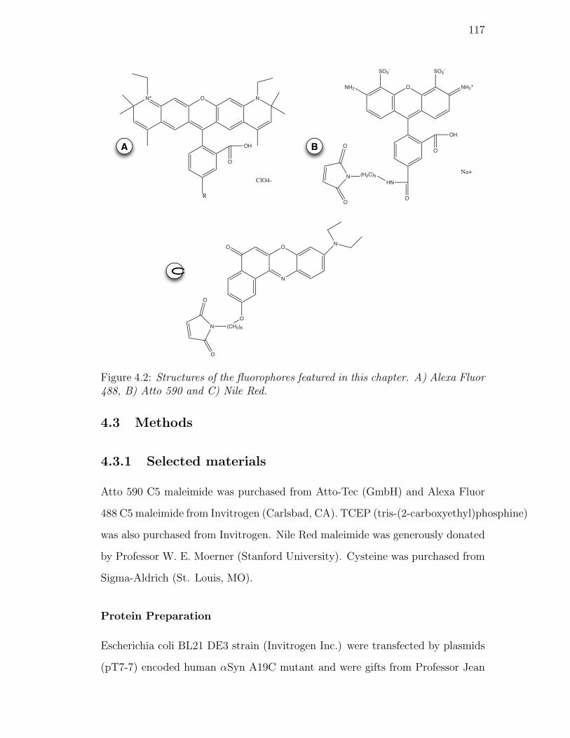
117
O
O
HNN
O
O
O
NH2+NH2
SO3- SO3
-
(H2C)5
OH
Na+
O
N
ON
O
(CH2)6N
O
O
O
O
OH
NN+
R
ClO4-
BA
C
Figure 4.2: Structures of the fluorophores featured in this chapter. A) Alexa Fluor488, B) Atto 590 and C) Nile Red.
4.3 Methods
4.3.1 Selected materials
Atto 590 C5 maleimide was purchased from Atto-Tec (GmbH) and Alexa Fluor
488 C5 maleimide from Invitrogen (Carlsbad, CA). TCEP (tris-(2-carboxyethyl)phosphine)
was also purchased from Invitrogen. Nile Red maleimide was generously donated
by Professor W. E. Moerner (Stanford University). Cysteine was purchased from
Sigma-Aldrich (St. Louis, MO).
Protein Preparation
Escherichia coli BL21 DE3 strain (Invitrogen Inc.) were transfected by plasmids
(pT7-7) encoded human αSyn A19C mutant and were gifts from Professor Jean
118
Baum (Rutgers University). Expression and purification of mutant αSyn followed
published protocols. [15]
4.3.2 Protein conjugation
Invitrogen’s protocol for thio-reactive probes was followed for the protein conjuga-
tion of NR-αSyn, Alexa-αSyn and Atto-αSyn. We note several changes/preferences.
Buffer used 10 mM phosphate, pH 7.0. Dyes were dissolved in 50 µL, or less,
of DMSO. TCEP was used to reduce disulfide bonds. Bio-Gel P-10 (BioRad)
columns were used for removing unreacted dye. β-mercaptoethanol was used to
stop the reaction. Alexa-αSyn and Atto-αSyn were filtered through a 100 kDa
molecular weight cutoff filter prior to experiments. Final concentrations were
about 1 mg/mL.
4.3.3 Cysteine conjugation
Along with the above protocol alterations, Alexa/cysteine conjugation requires
special attention to remove excess reactants. For this reaction, a 10X molar excess
of cysteine to Alexa maleimide was used. Removal of free cysteine was performed
by dialyzing against buffer with a low binding 500 Da cutoff Spectra/Por CE
dialysis bag.
4.3.4 Fluorescence spectroscopy
Temperature steady-state emission spectra were taken on a Cary Eclipse spec-
trometer (Varian Inc.). Excitation was set to 493 nm, and emission was 505 to
600 nm. Slit widths were set to 5 nm.
Data was taken every 5 Co from 5 to 95 C, then back to 5 C at a rate of
1 Co/min.
119
Time-resolved fluorescence
TRF was measured by TCSPC. For NR-αSyn, the experimental set up has been
previously described [10]. Temperature was maintained by a Quantum North-
West TLC150 Peltier controller sample chamber (Spokane, WA). Three experi-
ments were performed by the NR-αSyn conjugate. First, emission lifetime was
monitored at nine different wavelengths (ranging from 635 to 715 nm) with a
10 nm slit while held at 37 C. Then NR emission was measured at 655 nm as
the temperature was increased. The experiment was repeated but observing at
690 nm. Temperatures used were 15, 25, 37, 50, and 75 C.
For Alexa-cys, Alexa-αSyn and Atto-αSyn conjugates, experimental setup
was the same except that the Spectra Physics Tsunami Ti:Sapphire laser was
operated in femtosecond mode. The laser was tuned to 450 nm (after frequency
doubling) for the Alexa-cys and Alexa-αSyn experiments. Alexa-cys emission was
monitored at 516 nm with a 10 nm slit at 15, 25, 37, 50, and 75 C. The emission
for the Alexa-αSyn was collected in similar fashion, except that temperatures
ranged from 5 to 85 C, every ten degrees.
The absorption maximum of Atto-αSyn is at 593 nm and is well outside the
tunable range of the mid-range (M) optics set. Instead, a 400 nm excitation
beam was used where there is a small absorption band, most likely the second
excited state S2. We assume that excitation into this band will result in a fast
relaxation process (tens of femtoseconds, perhaps) to the first excited state, S1,
then radiatively emit back to the ground state, S0. Emission was monitored at
635 nm with a 10 nm slit and ranged from 10 to 90 C, every ten degrees.
Single molecule imaging
Two NR-αSyn samples were prepared for imaging: time-zero and after 8 days of
incubation at 37 C. These samples were diluted to 100 pM, and 20 µL of sample
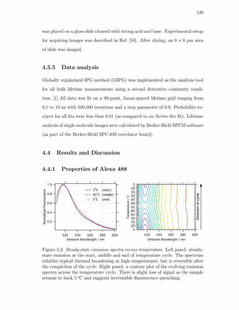
120
was placed on a glass slide cleaned with strong acid and base. Experimental setup
for acquiring images was described in Ref. [10]. After drying, an 8 × 8 µm area
of slide was imaged.
4.3.5 Data analysis
Globally regularized IPG method (GIPG) was implemented as the analysis tool
for all bulk lifetime measurements using a second derivative continuity condi-
tion. [1] All data was fit on a 99-point, linear-spaced lifetime grid ranging from
0.1 to 10 ns with 500,000 iterations and a step parameter of 0.9. Probability-to-
reject for all fits were less than 0.01 (as compared to an Active Set fit). Lifetime
analysis of single molecule images were calculated by Becker-Hickl SPCM software
(as part of the Becker-Hickl SPC-630 correlator board).
4.4 Results and Discussion
4.4.1 Properties of Alexa 488
Direction of cycle
Figure 4.3: Steady-state emission spectra versus temperature. Left panel: steady-state emission at the start, middle and end of temperature cycle. The spectrumexhibits typical thermal broadening at high temperatures, but is reversible afterthe completion of the cycle. Right panel: a contour plot of the evolving emissionspectra across the temperature cycle. There is slight loss of signal as the samplereturns to back 5 C and suggests irreversible fluorescence quenching.
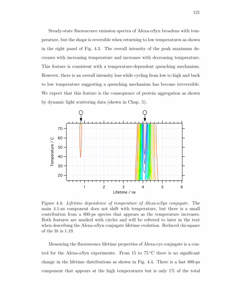
121
Steady-state fluorescence emission spectra of Alexa-αSyn broadens with tem-
perature, but the shape is reversible when returning to low temperatures as shown
in the right panel of Fig. 4.3. The overall intensity of the peak maximum de-
creases with increasing temperature and increases with decreasing temperature.
This feature is consistent with a temperature-dependent quenching mechanism.
However, there is an overall intensity loss while cycling from low to high and back
to low temperature suggesting a quenching mechanism has become irreversible.
We expect that this feature is the consequence of protein aggregation as shown
by dynamic light scattering data (shown in Chap. 5).
Figure 4.4: Lifetime dependence of temperature of Alexa-αSyn conjugate. Themain 4.1-ns component does not shift with temperature, but there is a smallcontribution from a 800-ps species that appears as the temperature increases.Both features are marked with circles and will be referred to later in the textwhen describing the Alexa-αSyn conjugate lifetime evolution. Reduced chi-squareof the fit is 1.19.
Measuring the fluorescence lifetime properties of Alexa-cys conjugate is a con-
trol for the Alexa-αSyn experiments. From 15 to 75 C there is no significant
change in the lifetime distributions as shown in Fig. 4.4. There is a fast 800-ps
component that appears at the high temperatures but is only 1% of the total
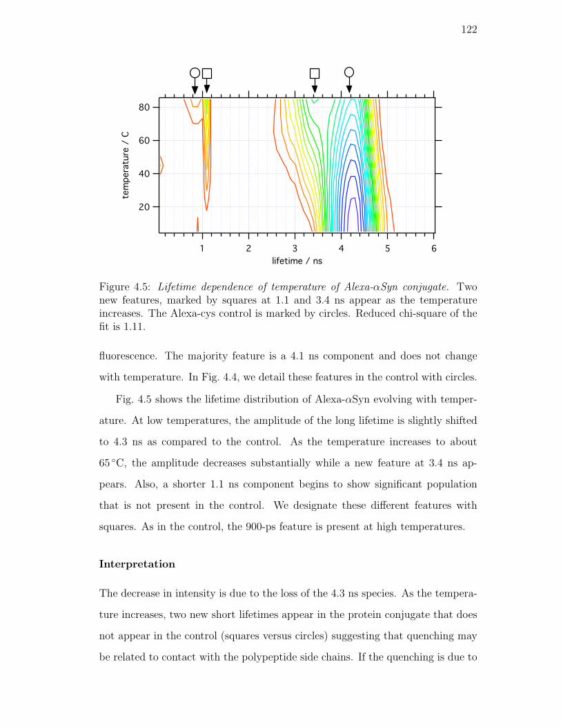
122
Figure 4.5: Lifetime dependence of temperature of Alexa-αSyn conjugate. Twonew features, marked by squares at 1.1 and 3.4 ns appear as the temperatureincreases. The Alexa-cys control is marked by circles. Reduced chi-square of thefit is 1.11.
fluorescence. The majority feature is a 4.1 ns component and does not change
with temperature. In Fig. 4.4, we detail these features in the control with circles.
Fig. 4.5 shows the lifetime distribution of Alexa-αSyn evolving with temper-
ature. At low temperatures, the amplitude of the long lifetime is slightly shifted
to 4.3 ns as compared to the control. As the temperature increases to about
65 C, the amplitude decreases substantially while a new feature at 3.4 ns ap-
pears. Also, a shorter 1.1 ns component begins to show significant population
that is not present in the control. We designate these different features with
squares. As in the control, the 900-ps feature is present at high temperatures.
Interpretation
The decrease in intensity is due to the loss of the 4.3 ns species. As the tempera-
ture increases, two new short lifetimes appear in the protein conjugate that does
not appear in the control (squares versus circles) suggesting that quenching may
be related to contact with the polypeptide side chains. If the quenching is due to
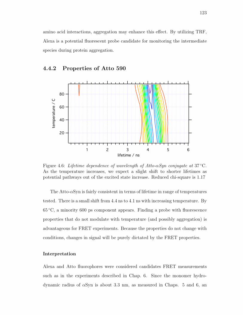
123
amino acid interactions, aggregation may enhance this effect. By utilizing TRF,
Alexa is a potential fluorescent probe candidate for monitoring the intermediate
species during protein aggregation.
4.4.2 Properties of Atto 590
80
60
40
20
tem
pera
ture
/ C
654321
lifetime / ns
Figure 4.6: Lifetime dependence of wavelength of Atto-αSyn conjugate at 37 C.As the temperature increases, we expect a slight shift to shorter lifetimes aspotential pathways out of the excited state increase. Reduced chi-square is 1.17
The Atto-αSyn is fairly consistent in terms of lifetime in range of temperatures
tested. There is a small shift from 4.4 ns to 4.1 ns with increasing temperature. By
65 C, a minority 600 ps component appears. Finding a probe with fluorescence
properties that do not modulate with temperature (and possibly aggregation) is
advantageous for FRET experiments. Because the properties do not change with
conditions, changes in signal will be purely dictated by the FRET properties.
Interpretation
Alexa and Atto fluorophores were considered candidates FRET measurements
such as in the experiments described in Chap. 6. Since the monomer hydro-
dynamic radius of αSyn is about 3.3 nm, as measured in Chaps. 5 and 6, an
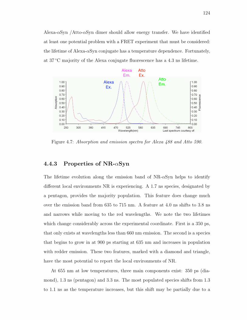
124
Alexa-αSyn /Atto-αSyn dimer should allow energy transfer. We have identified
at least one potential problem with a FRET experiment that must be considered:
the lifetime of Alexa-αSyn conjugate has a temperature dependence. Fortunately,
at 37 C majority of the Alexa conjugate fluorescence has a 4.3 ns lifetime.
Alexa
Em.
Atto
Ex.
Alexa
Ex.
Atto
Em.
Figure 4.7: Absorption and emission spectra for Alexa 488 and Atto 590.
4.4.3 Properties of NR-αSyn
The lifetime evolution along the emission band of NR-αSyn helps to identify
different local environments NR is experiencing. A 1.7 ns species, designated by
a pentagon, provides the majority population. This feature does change much
over the emission band from 635 to 715 nm. A feature at 4.0 ns shifts to 3.8 ns
and narrows while moving to the red wavelengths. We note the two lifetimes
which change considerably across the experimental coordinate. First is a 350 ps,
that only exists at wavelengths less than 660 nm emission. The second is a species
that begins to grow in at 900 ps starting at 635 nm and increases in population
with redder emission. These two features, marked with a diamond and triangle,
have the most potential to report the local environments of NR.
At 655 nm at low temperatures, three main components exist: 350 ps (dia-
mond), 1.3 ns (pentagon) and 3.3 ns. The most populated species shifts from 1.3
to 1.1 ns as the temperature increases, but this shift may be partially due to a
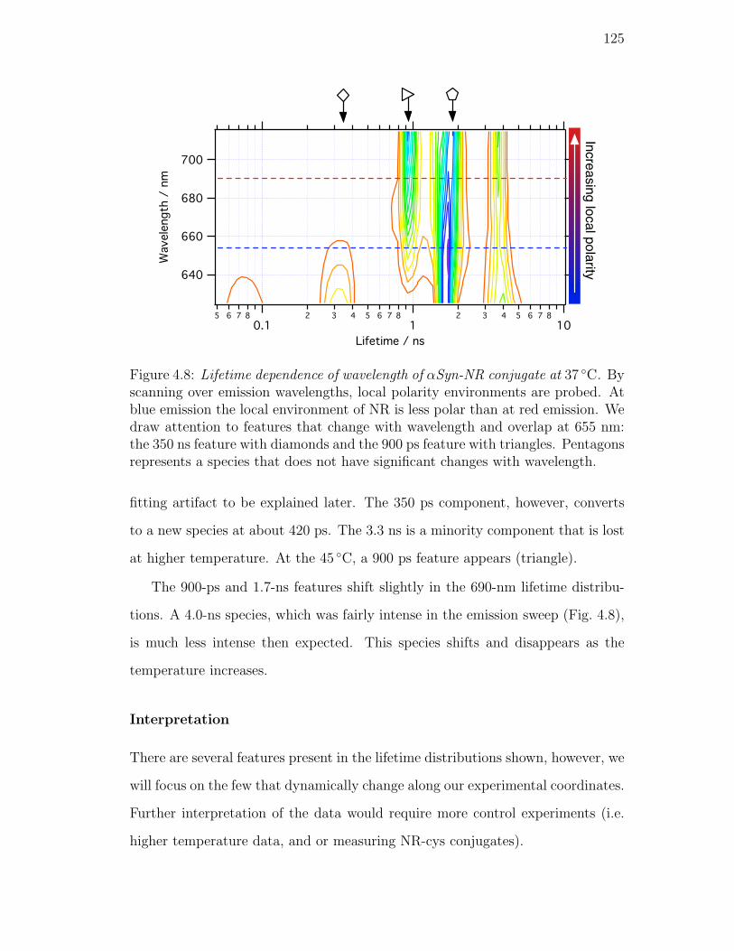
125
Increasing local polarity
Figure 4.8: Lifetime dependence of wavelength of αSyn-NR conjugate at 37 C. Byscanning over emission wavelengths, local polarity environments are probed. Atblue emission the local environment of NR is less polar than at red emission. Wedraw attention to features that change with wavelength and overlap at 655 nm:the 350 ns feature with diamonds and the 900 ps feature with triangles. Pentagonsrepresents a species that does not have significant changes with wavelength.
fitting artifact to be explained later. The 350 ps component, however, converts
to a new species at about 420 ps. The 3.3 ns is a minority component that is lost
at higher temperature. At the 45 C, a 900 ps feature appears (triangle).
The 900-ps and 1.7-ns features shift slightly in the 690-nm lifetime distribu-
tions. A 4.0-ns species, which was fairly intense in the emission sweep (Fig. 4.8),
is much less intense then expected. This species shifts and disappears as the
temperature increases.
Interpretation
There are several features present in the lifetime distributions shown, however, we
will focus on the few that dynamically change along our experimental coordinates.
Further interpretation of the data would require more control experiments (i.e.
higher temperature data, and or measuring NR-cys conjugates).
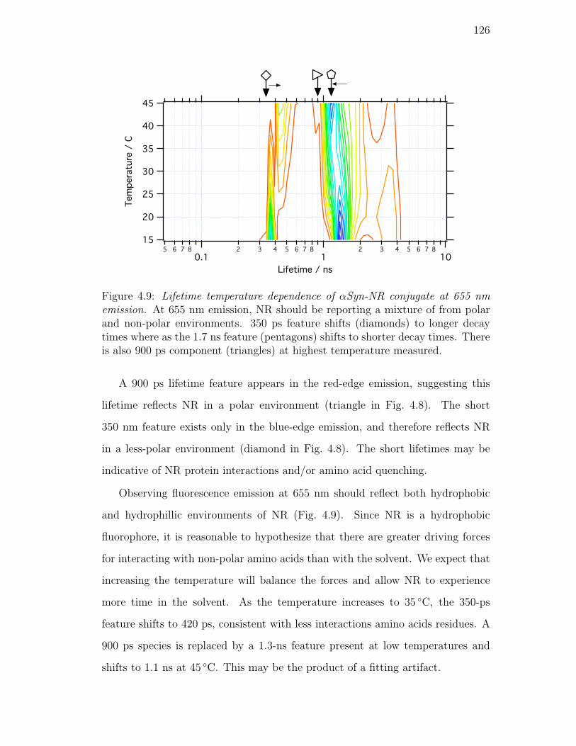
126
Figure 4.9: Lifetime temperature dependence of αSyn-NR conjugate at 655 nmemission. At 655 nm emission, NR should be reporting a mixture of from polarand non-polar environments. 350 ps feature shifts (diamonds) to longer decaytimes where as the 1.7 ns feature (pentagons) shifts to shorter decay times. Thereis also 900 ps component (triangles) at highest temperature measured.
A 900 ps lifetime feature appears in the red-edge emission, suggesting this
lifetime reflects NR in a polar environment (triangle in Fig. 4.8). The short
350 nm feature exists only in the blue-edge emission, and therefore reflects NR
in a less-polar environment (diamond in Fig. 4.8). The short lifetimes may be
indicative of NR protein interactions and/or amino acid quenching.
Observing fluorescence emission at 655 nm should reflect both hydrophobic
and hydrophillic environments of NR (Fig. 4.9). Since NR is a hydrophobic
fluorophore, it is reasonable to hypothesize that there are greater driving forces
for interacting with non-polar amino acids than with the solvent. We expect that
increasing the temperature will balance the forces and allow NR to experience
more time in the solvent. As the temperature increases to 35 C, the 350-ps
feature shifts to 420 ps, consistent with less interactions amino acids residues. A
900 ps species is replaced by a 1.3-ns feature present at low temperatures and
shifts to 1.1 ns at 45 C. This may be the product of a fitting artifact.
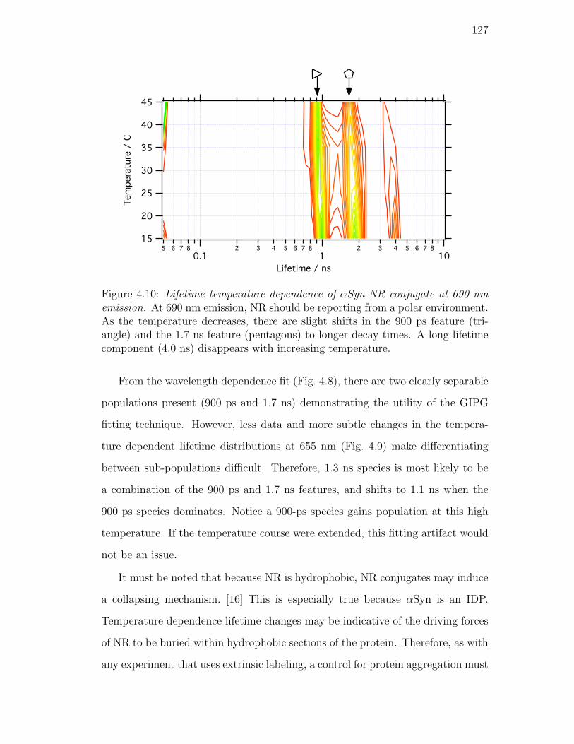
127
Figure 4.10: Lifetime temperature dependence of αSyn-NR conjugate at 690 nmemission. At 690 nm emission, NR should be reporting from a polar environment.As the temperature decreases, there are slight shifts in the 900 ps feature (tri-angle) and the 1.7 ns feature (pentagons) to longer decay times. A long lifetimecomponent (4.0 ns) disappears with increasing temperature.
From the wavelength dependence fit (Fig. 4.8), there are two clearly separable
populations present (900 ps and 1.7 ns) demonstrating the utility of the GIPG
fitting technique. However, less data and more subtle changes in the tempera-
ture dependent lifetime distributions at 655 nm (Fig. 4.9) make differentiating
between sub-populations difficult. Therefore, 1.3 ns species is most likely to be
a combination of the 900 ps and 1.7 ns features, and shifts to 1.1 ns when the
900 ps species dominates. Notice a 900-ps species gains population at this high
temperature. If the temperature course were extended, this fitting artifact would
not be an issue.
It must be noted that because NR is hydrophobic, NR conjugates may induce
a collapsing mechanism. [16] This is especially true because αSyn is an IDP.
Temperature dependence lifetime changes may be indicative of the driving forces
of NR to be buried within hydrophobic sections of the protein. Therefore, as with
any experiment that uses extrinsic labeling, a control for protein aggregation must
128
be performed on the wild type protein with an independent measure of amyloid
growth.
4.4.4 SM
Single molecule imaging allows the separation of lifetimes of different sized NR-
αSyn aggregates found in the bulk solution. Monitoring the discrete drops in
intensity of an imaged particle for each successive scan, it is possible to identify
the number of probes per spot. Coupled with lifetime analysis, a lifetime can be
designated for a particular size or type of aggregate. [10].
The single molecule images shown in Figs. 4.11 and 4.12 are of time-zero and
day 8 NR-αSyn, respectively, and is colored by lifetime. In panel A, there are
several spots with lifetimes ranging from 2 to 4 ns. After a second scan (panel
B), several of these features go dark including the one inside the circle. Panel C
represents a third pass; most of the fluorescence has disappeared except for the
blue spot (4 to 6 ns) in the white box. Panel D reveals recovery by some molecules
(for example, on the far left), but the blue spot has almost disappeared. After 8
days of incubation, fibrils have formed as determined by atomic force microscopy
(data not shown). Typical fluorescence of a fibril is shown in Fig. 4.12. The
lifetime for a fibril is consistently short, i.e. 0.4 to 1.0 ns.
Interpretation
Monomers, aggregates, and fibrils can be distinguished by their NR lifetimes using
single molecule fluorescence. Features with similar low intensity and photobleach
by scan B, such as in the white circle shown panel A to B in Fig. 4.11, suggest
these molecules are monomeric NR-αSyn. The lifetime for the monomer ranges
from 2 to 4 ns suggesting the environment allows the non-polar regions of protein
to be available to NR even though it is partially exposed. Oligomers are round
and amorphous, take multiple steps to photobleach, and exhibit longer lifetimes
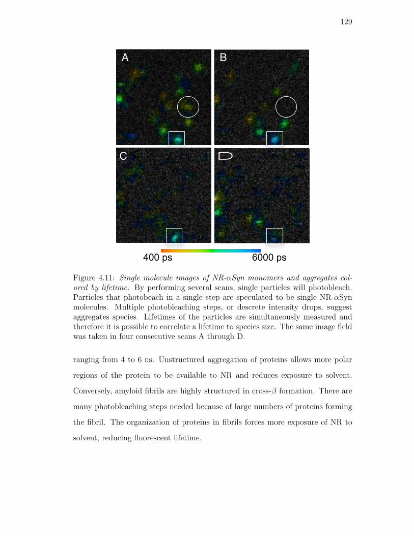
129
A B
C D
400 ps 6000 ps
Figure 4.11: Single molecule images of NR-αSyn monomers and aggregates col-ored by lifetime. By performing several scans, single particles will photobleach.Particles that photobeach in a single step are speculated to be single NR-αSynmolecules. Multiple photobleaching steps, or descrete intensity drops, suggestaggregates species. Lifetimes of the particles are simultaneously measured andtherefore it is possible to correlate a lifetime to species size. The same image fieldwas taken in four consecutive scans A through D.
ranging from 4 to 6 ns. Unstructured aggregation of proteins allows more polar
regions of the protein to be available to NR and reduces exposure to solvent.
Conversely, amyloid fibrils are highly structured in cross-β formation. There are
many photobleaching steps needed because of large numbers of proteins forming
the fibril. The organization of proteins in fibrils forces more exposure of NR to
solvent, reducing fluorescent lifetime.
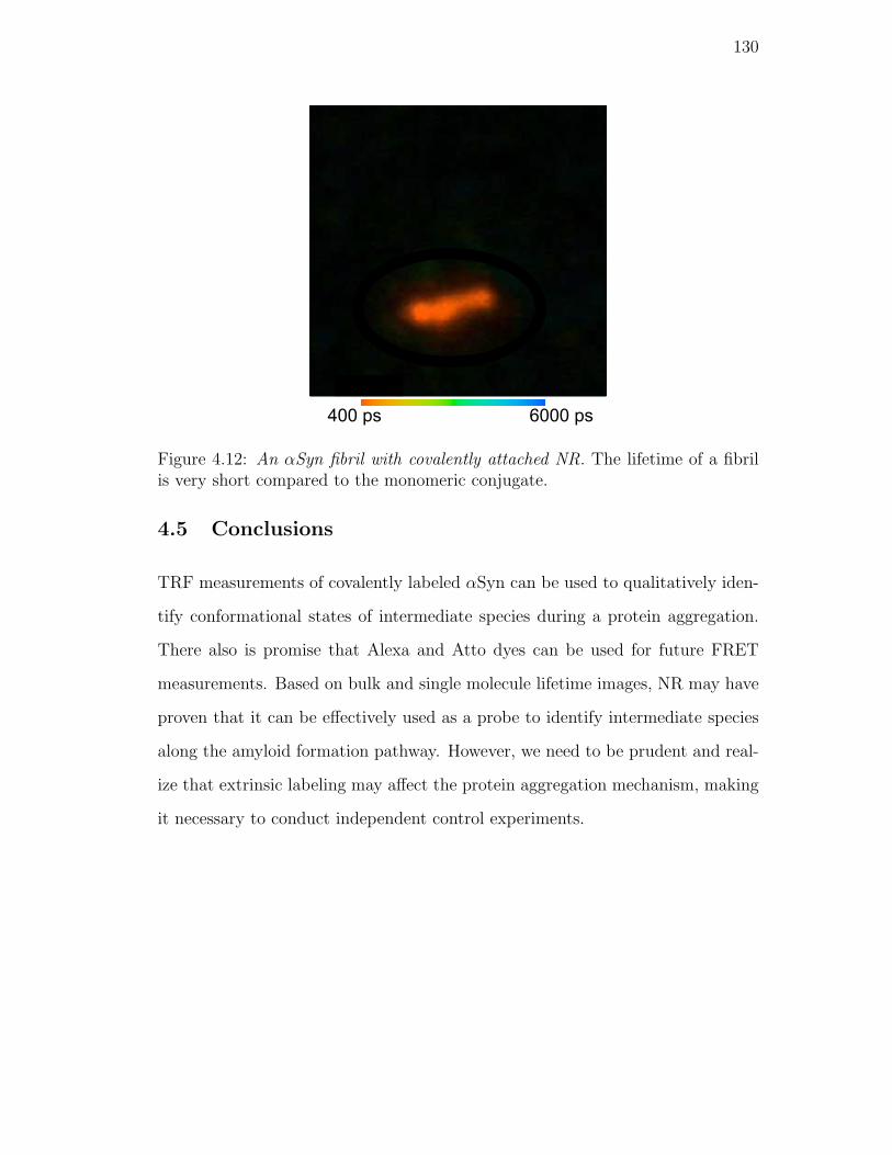
130
400 ps 6000 ps
Figure 4.12: An αSyn fibril with covalently attached NR. The lifetime of a fibrilis very short compared to the monomeric conjugate.
4.5 Conclusions
TRF measurements of covalently labeled αSyn can be used to qualitatively iden-
tify conformational states of intermediate species during a protein aggregation.
There also is promise that Alexa and Atto dyes can be used for future FRET
measurements. Based on bulk and single molecule lifetime images, NR may have
proven that it can be effectively used as a probe to identify intermediate species
along the amyloid formation pathway. However, we need to be prudent and real-
ize that extrinsic labeling may affect the protein aggregation mechanism, making
it necessary to conduct independent control experiments.
131
References
[1] Jason T. Giurleo and David S. Talaga. Global fitting without a global model:Regularization based on the continuity of the evolution of parameter distri-butions. The Journal of Chemical Physics, 128:114114–(1–18), 2008.
[2] Chirlmin Joo, Hamza Balci, Yuji Ishitsuka, Chittanon Buranachai, andTaekjip Ha. Advances in single-molecule fluorescence methods for molec-ular biology. Annual Review of Biochemistry, 77:51–76, 2008.
[3] Ashok A. Deniz, Samrat Mukhopadhyay, and Edward A. Lemke. Single-molecule biophysics: at the interface of biology, physics and chemistry. J. R.Soc. Interface, 5:15–45, 2008.
[4] Joseph R. Lakowicz. Principles of Fluorescence Spectroscopy. Plenum PubCorp, 1999.
[5] Victor Munoz. Conformational dynamics and ensembles in protein folding.Annu. Rev. Biophys. Biomol. Struct., 36:395–412, 2007.
[6] A. Keith Dunker, J. David Lawson, Celeste J. Brown, Ryan M. Williams,Pedro Romero, Jeong S. Oh, Christopher J. Oldfield, Andrew M. Campen,Catherine M. Ratliff, Kerry W. Hipps, Juan Ausio, Mark S. Nissen, RaymondReeves, ChulHee Kang, Charles R. Kissinger, Robert W. Bailey, Michael D.Griswold, Wah Chiu, Ethan C. Garner, , and Zoran Obradovic. Intrinsicallydisordered protein. Journal of Molecular Graphics and Modelling, 19:26–59,2001.
[7] Kelly A. Conway, Seung-Jae Lee, Jean-Christophe Rochet, Tomas T. Ding,Robin E. Williamson, and Peter T. Lansbury Jr. Acceleration of oligomer-ization, not fibrillization, is a shared property of both α-synuclein mutationslinked to early-onset parkinson’s disease: Implications for pathogenesis andtherapy. Proc. Nat. Acad. Sci., 97:571–576, 2000.
[8] Byron Caughey and Peter T. Lansbury Jr. Protofibrils, pores, fibrils, andneurodegeneration: Separating the responsible protein aggregates from theinnocent bystanders. Annu. Rev. Neurosci., 26:267–298, 2003.
[9] Jason T. Giurleo, Xianglan He, and David S. Talaga. β-lactoglobulin assem-bles into amyloid through sequential aggregated intermediates. J. Mol. Bio.,381:1332–1348, 2008.

132
[10] Troy C. Messina, Hiyun Kim, Jason T. Giurleo, and David S. Talaga. Hiddenmarkov model analysis of multichromophore photobleaching. J. Phys. Chem.B, 110:16366–16376, 2006.
[11] Dan L. Sackett, Jay R. Knutsonf, and J. Wolff. Hydrophobic surfaces oftubulin probed by time-resolved and steady-state fluorescence of nile red. J.Bio. Chem., 265:14699–14906, 1990.
[12] Soumi Mukherjee, H. Raghuraman, and Amitabha Chattopadhyay. Mem-brane localization and dynamics of nile red: Effect of cholesterol. Biochimicaet Biophysica Acta, 1768:59–66, 2007.
[13] Yanwen Hou, Angela M. Bardo, Cruz Martinez, and Daniel A. Higgins.Characterization of molecular scale environments in polymer films by sin-gle molecule spectroscopy. J. Phys. Chem. B, 104:212–219, 2000.
[14] So Yeon Kim, Alexander N. Semyonov, Robert J. Twieg, Arthur L. Horwich,Judith Frydman, and W. E. Moerner. Probing the sequence of conforma-tionally induced polarity changes in the molecular chaperonin groel withfluorescence spectroscopy. J. Phys. Chem. B, 109:24517–24525, 2005.
[15] Paul H. Weinreb, Weiguo Zhen, Anna W. Poon, Kelly A. Conway, and Pe-ter T. Lansbury Jr. Nacp, a protein implicated in alzheimer’s disease andlearning, is natively unfolded. Biochemistry, 35:13709–13715, 1996.
[16] David W. Miller and Ken A. Dill. Ligand binding to proteins: The bindinglandscape model. Protein Science, 6:2166–2179, 1997.
133
Chapter 5
Thermodynamic studies of α-synuclein
5.1 Summary
α-Synuclein is an intrinsically disordered protein found in the brain and is impli-
cated in Parkinson’s disease. It has no known function but its primary sequence
is highly conserved across species. Understanding its monomeric conformational
properties may led to elucidating its function. Little has been published on the
thermodynamic states of α-synuclein. We show that there are subtle spectroscopic
transitions present in the ellipticity and 287 nm absorption. The spectroscopic
transitions are connected to the microscopic states of the system through the
partition function. We take advantage of the partition function to calculate the
temperature at which a transition occurs and speculate how these transitions
relate to secondary and tertiary conformational changes.
5.2 Introduction
Disease
Parkinson’s disease (PD) affects over half-a-million people in the the United
States. [1] Clinical symptoms of PD include characteristic resting tremors and in-
ability to control the extent of their movements. α-Synuclein (αSyn) is the main
component of the intracytoplasmic proteinaceous deposits found in the brains of
70 to 80% of patients clinically diagnosed with PD. [1]. Neuronal inclusion bodies,
called Lewy bodies, contain aggregated αSyn in the form of fibrils which exhibit
134
cross-β quaternary structure. However, pathological implications of Lewy bodies
have been questioned and has led to research on the pre-fibrillar oligomeric aggre-
gation states of αSyn. [2, 3, 1] One of the interesting features of αSyn is that it
belongs to a class of protein that is intrinsically disordered. In an intrinsically dis-
ordered protein, or IDP, there is no evidence of a single native structure. Study-
ing the aggregation mechanism of αSyn begins with a basic understanding of the
properties of the monomeric protein.
Intrinsically disordered protein
IDPs can be characterized by using X-ray crystallography, NMR spectroscopy,
circular dichroism spectroscopy, protease digestion, and hydrodynamic radius de-
termination. Researchers using X-ray crystallography were the first to discover
there were segments of a protein that had indiscernible structure but were abso-
lutely necessary for function. [4] Because of the dynamic nature of NMR, it since
become a powerful technique in recognizing segmental conformational ambigu-
ity. [5]
The structure-function paradigm has become a cornerstone of protein struc-
ture prediction and structural genomics. [4] The relationship between primary
sequence → 3 dimensional structure → function has helped structural biologists
to understand features of protein when one or two parts are unknown. However,
the obvious prerequisite is that the protein has to have either a function or a
native structure to be useful in this paradigm.
The function of αSyn in the brain is poorly understood [2, 1], but it is known
that the expression levels in the brain are high [6], and it is highly conserved across
species. [7] We presently aware of only two thermodynamic studies of αSyn but
they were conducted in the presence of sodium dodecyl sulfate [8] and phospho-
lipid vesicles. [9] Remeta and Minetti have recently conducted differential scan-
ning calorimetry experiment at high concentrations of αSyn, but have not seen
135
any sign of an enthalpic transition. (personal communication).
Two thermodynamic states
Two-state transitions are often used to describe protein folding mechanisms when
no intermediate species are observed. Observing versus not observing intermedi-
ates when these species do exist may be the consequence of several factors. For
example, the experimental timescale needs to be comparable to the lifetime of
species. Also, the signal needs to be sensitive to intermediate species. Ensem-
ble averaging of the signal adds another confounding complication to the differ-
entiating intermediate species. Single molecule spectroscopy has been used to
circumvent the last condition. [10, 11, 12] Discussions concerning protein folding
transitions are described in detail elsewhere. [13, 14, 15, 16].
Since αSyn has very little intrinsic structure, the classic folding paradigm
innately does not apply. However, when αSyn is heated, certain spectroscopic
observables modulate. A simple way to describe the change in the observable
is to consider the protein is moving from one thermodynamic state to another.
This is in spite of not having a single native state conformation. Moving from
an intrinsically disordered to state to an even greater, or extrinsically, disordered
state, there are low expectations for a large observable transition. Because of this
the nuances of the transitions are not explicitly discussed here.
The partition function connects the macroscopic thermodynamic properties
with the microscopic states. The partition function can then be formulated such
that the multiplicity of the upper state and the energy gap are parameters which
fit the spectroscopic observables. If the data supports greater degeneracy in the
upper state, this suggests a more cooperative transition. The energy and the
“cooperativity” parameters can be used to predict the transition temperature,
Tm, as the system moves from one spectroscopic state to another.
Three biophysical techniques are used to monitor the thermodynamics of
136
αSyn. Circular dichroism (CD) is utilized to monitor the evolution of mean
residue molar ellipticity and give clues of overall secondary structure changes.
Dynamic light scattering (DLS) is used to follow the average change in hydro-
dynamic radius (RH). Lastly, modulation in the ultraviolet absorption (UV)
at 287 nm is often indicative of some tertiary structural changes of the tyrosyl
moieties. [17] UV measurements in this range can be confounded by absorption
overlap with tryptophan; fortunately, αSyn does not have tryptophan in its pri-
mary sequence. These techniques may lay down the ground work for future more
complicated experiments, such as NMR and computer simulations, which can
theoretically yield information on a residue-by-residue basis.
5.3 Methods
5.3.1 Preparation and Purification
Escherichia coli BL21 DE3 strain (Invitrogen Inc.) were transfected by plas-
mids (pT7-7) encoded human αSyn and was a gift from Professor Jean Baum
(Rutgers University, Piscataway, NJ). Expression and purification followed pub-
lished protocols. [18] αSyn was lyophilized and stored until it was reconstituted
to 1.0 mg/mL in 10 mM phosphate, pH 7.0 buffer at the time of the experiment.
To remove the insoluble and soluble aggregates from protein solution for any ex-
periment, the sample was filtered through a Microcon 100 kDa molecular weight
cutoff filter (YM-100, Millipore).
5.3.2 UV
Temperature-dependent UV melting experiments were performed on an Aviv
Model 14 UV/Vis spectrophotometer (Aviv Biomedical Inc., Lakewood, NJ).
Samples in quartz cuvettes of 1.0 cm pathlength were heated in the thermostatted
137
sample compartment over the temperature range of 0 to 100 C. The absorbance
at 287 nm was recorded at 0.5 Co increments following integration for 10 seconds
to monitor the absorbance changes as a function of temperature. Though a pre-
liminary melt on the VARIAN was performed at 250, 280, 287, and 350 nm, only
the 287 nm absorption had a visible transition.
5.3.3 DLS
Round borosilicate glass cuvettes (Kimble Glass) were for the DLS measurement.
In order to minimize dust contamination, the cuvette was rinsed with Millipore
water. It was then placed in a micro-centrifuge, inverted (open-side face-down),
then spun dry and stored face down. After the sample was quickly and carefully
added to the cuvette, it was covered with transparent tape to keep it dust-free,
then wrapped in Parafilm for an additional seal.
Fluctuations of scattered light intensity were measured using a homodyne
technique. At a particular temperature, T , the intensity correlation function
g2(t, T ), was measured by a modified Nicomp Model 380 Particle Size Analyzer
from Particle Sizing Systems. Scattered light from the incident laser, λ=532 nm,
was collected orthogonally, θ=90. The system employs a linearly-scaled 64-
channel digital autocorrelator. The native autocorrelator was bypassed by an
ALV-6010 Multi-Tau autocorrelator (ALV-GmbH, Langen, Germany) for the max-
imum possible statistical accuracy across several orders of magnitude in decay
time. [19]
DLS correlation functions were fit using regularized GIPG with a linear con-
tinuity condition. [20] The Laplace transform was performed using a grid of ex-
ponential decay times. A particle’s decay time is related to the translational
diffusion constant though the scattering vector, q, such that D = Γ/q2, where
q = 4nπ/λ sin(θ/2), n is the refractive index. The diffusion constant can then
be converted to a Stokes-hydrodynamic radius (RH) using the Stokes-Einstein
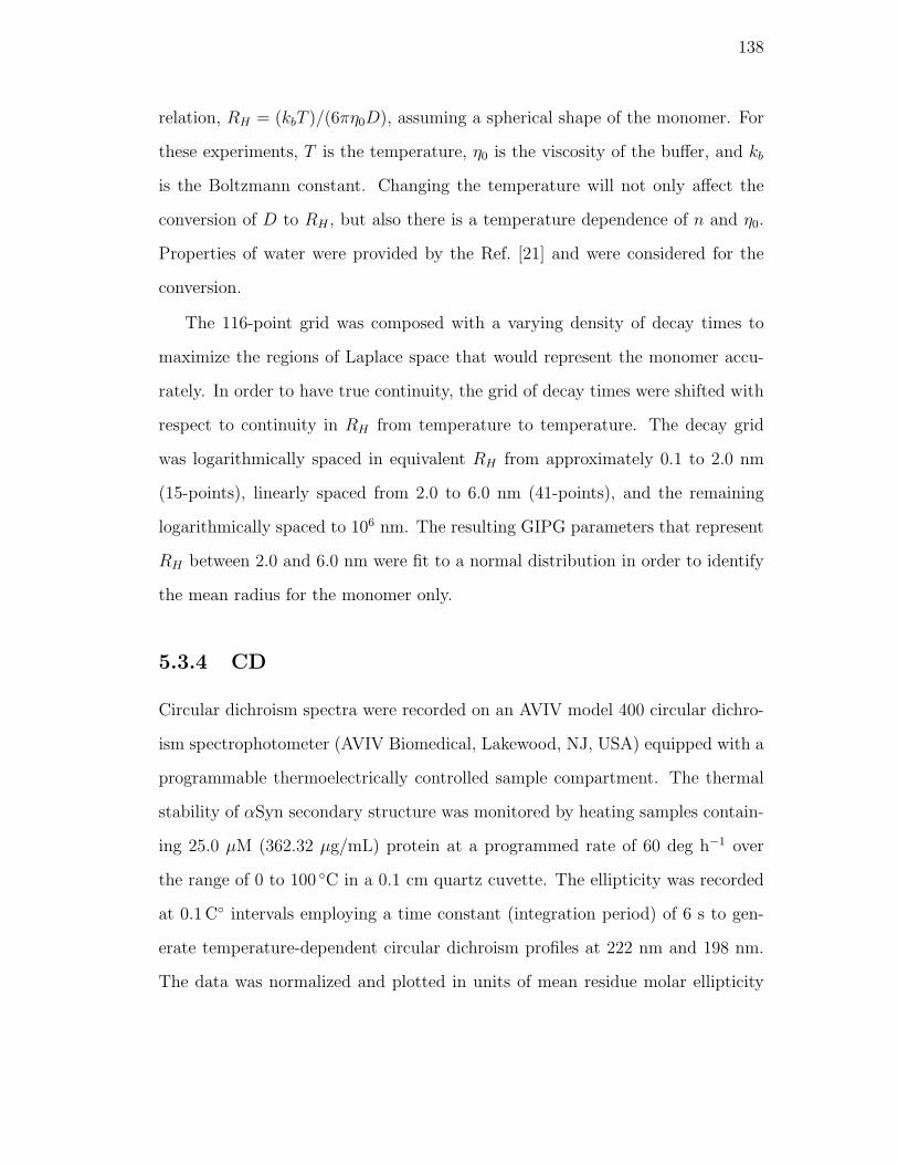
138
relation, RH = (kbT )/(6πη0D), assuming a spherical shape of the monomer. For
these experiments, T is the temperature, η0 is the viscosity of the buffer, and kb
is the Boltzmann constant. Changing the temperature will not only affect the
conversion of D to RH , but also there is a temperature dependence of n and η0.
Properties of water were provided by the Ref. [21] and were considered for the
conversion.
The 116-point grid was composed with a varying density of decay times to
maximize the regions of Laplace space that would represent the monomer accu-
rately. In order to have true continuity, the grid of decay times were shifted with
respect to continuity in RH from temperature to temperature. The decay grid
was logarithmically spaced in equivalent RH from approximately 0.1 to 2.0 nm
(15-points), linearly spaced from 2.0 to 6.0 nm (41-points), and the remaining
logarithmically spaced to 106 nm. The resulting GIPG parameters that represent
RH between 2.0 and 6.0 nm were fit to a normal distribution in order to identify
the mean radius for the monomer only.
5.3.4 CD
Circular dichroism spectra were recorded on an AVIV model 400 circular dichro-
ism spectrophotometer (AVIV Biomedical, Lakewood, NJ, USA) equipped with a
programmable thermoelectrically controlled sample compartment. The thermal
stability of αSyn secondary structure was monitored by heating samples contain-
ing 25.0 µM (362.32 µg/mL) protein at a programmed rate of 60 deg h−1 over
the range of 0 to 100 C in a 0.1 cm quartz cuvette. The ellipticity was recorded
at 0.1 C intervals employing a time constant (integration period) of 6 s to gen-
erate temperature-dependent circular dichroism profiles at 222 nm and 198 nm.
The data was normalized and plotted in units of mean residue molar ellipticity
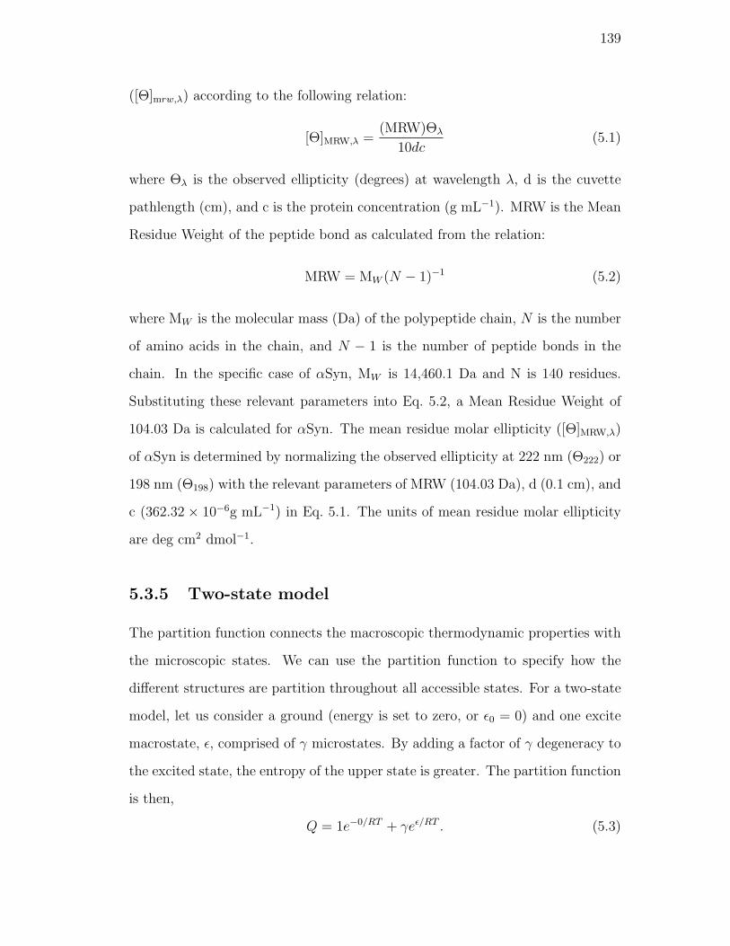
139
([Θ]mrw,λ) according to the following relation:
[Θ]MRW,λ =(MRW)Θλ
10dc(5.1)
where Θλ is the observed ellipticity (degrees) at wavelength λ, d is the cuvette
pathlength (cm), and c is the protein concentration (g mL−1). MRW is the Mean
Residue Weight of the peptide bond as calculated from the relation:
MRW = MW (N − 1)−1 (5.2)
where MW is the molecular mass (Da) of the polypeptide chain, N is the number
of amino acids in the chain, and N − 1 is the number of peptide bonds in the
chain. In the specific case of αSyn, MW is 14,460.1 Da and N is 140 residues.
Substituting these relevant parameters into Eq. 5.2, a Mean Residue Weight of
104.03 Da is calculated for αSyn. The mean residue molar ellipticity ([Θ]MRW,λ)
of αSyn is determined by normalizing the observed ellipticity at 222 nm (Θ222) or
198 nm (Θ198) with the relevant parameters of MRW (104.03 Da), d (0.1 cm), and
c (362.32 × 10⁻⁶g mL−1) in Eq. 5.1. The units of mean residue molar ellipticity
are deg cm2 dmol−1.
5.3.5 Two-state model
The partition function connects the macroscopic thermodynamic properties with
the microscopic states. We can use the partition function to specify how the
different structures are partition throughout all accessible states. For a two-state
model, let us consider a ground (energy is set to zero, or ε0 = 0) and one excite
macrostate, ε, comprised of γ microstates. By adding a factor of γ degeneracy to
the excited state, the entropy of the upper state is greater. The partition function
is then,
Q = 1e−0/RT + γeε/RT . (5.3)
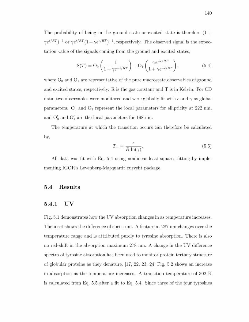
140
The probability of being in the ground state or excited state is therefore (1 +
γeε/RT )−1 or γeε/RT (1 +γeε/RT )−1, respectively. The observed signal is the expec-
tation value of the signals coming from the ground and excited states,
S(T ) = O0
(1
1 + γe−ε/RT
)+ O1
(γe−ε/RT
1 + γe−ε/RT
). (5.4)
where O0 and O1 are representative of the pure macrostate observables of ground
and excited states, respectively. R is the gas constant and T is in Kelvin. For CD
data, two observables were monitored and were globally fit with ε and γ as global
parameters. O0 and O1 represent the local parameters for ellipticity at 222 nm,
and O′0 and O′1 are the local parameters for 198 nm.
The temperature at which the transition occurs can therefore be calculated
by,
Tm =ε
R ln(γ). (5.5)
All data was fit with Eq. 5.4 using nonlinear least-squares fitting by imple-
menting IGOR’s Levenberg-Marquardt curvefit package.
5.4 Results
5.4.1 UV
Fig. 5.1 demonstrates how the UV absorption changes in as temperature increases.
The inset shows the difference of spectrum. A feature at 287 nm changes over the
temperature range and is attributed purely to tyrosine absorption. There is also
no red-shift in the absorption maximum 278 nm. A change in the UV difference
spectra of tyrosine absorption has been used to monitor protein tertiary structure
of globular proteins as they denature. [17, 22, 23, 24] Fig. 5.2 shows an increase
in absorption as the temperature increases. A transition temperature of 302 K
is calculated from Eq. 5.5 after a fit to Eq. 5.4. Since three of the four tyrosines
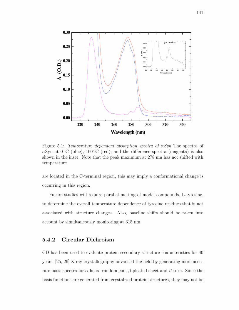
141
220 240 260 280 300 320 340
0.00
0.05
0.10
0.15
0.20
0.25
0.30
A (O.D.)
Wavelength (nm)
200 220 240 260 280 300 320 340
0.00
0.01
0.02
0.03
0.04
0.05 peak ~ 287-288 nm
A (O.D.)
Wavelength (nm)
Figure 5.1: Temperature dependent absorption spectra of αSyn The spectra ofαSyn at 0 C (blue), 100 C (red), and the difference spectra (magenta) is alsoshown in the inset. Note that the peak maximum at 278 nm has not shifted withtemperature.
are located in the C-terminal region, this may imply a conformational change is
occurring in this region.
Future studies will require parallel melting of model compounds, L-tyrosine,
to determine the overall temperature-dependence of tyrosine residues that is not
associated with structure changes. Also, baseline shifts should be taken into
account by simultaneously monitoring at 315 nm.
5.4.2 Circular Dichroism
CD has been used to evaluate protein secondary structure characteristics for 40
years. [25, 26] X-ray crystallography advanced the field by generating more accu-
rate basis spectra for α-helix, random coil, β-pleated sheet and β-turn. Since the
basis functions are generated from crystalized protein structures, they may not be
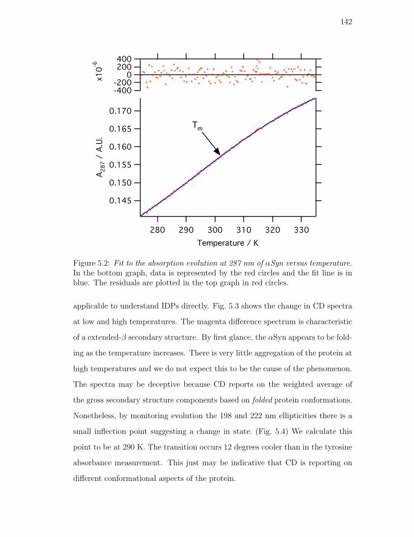
142
Tm
Figure 5.2: Fit to the absorption evolution at 287 nm of αSyn versus temperature.In the bottom graph, data is represented by the red circles and the fit line is inblue. The residuals are plotted in the top graph in red circles.
applicable to understand IDPs directly. Fig. 5.3 shows the change in CD spectra
at low and high temperatures. The magenta difference spectrum is characteristic
of a extended-β secondary structure. By first glance, the αSyn appears to be fold-
ing as the temperature increases. There is very little aggregation of the protein at
high temperatures and we do not expect this to be the cause of the phenomenon.
The spectra may be deceptive because CD reports on the weighted average of
the gross secondary structure components based on folded protein conformations.
Nonetheless, by monitoring evolution the 198 and 222 nm ellipticities there is a
small inflection point suggesting a change in state. (Fig. 5.4) We calculate this
point to be at 290 K. The transition occurs 12 degrees cooler than in the tyrosine
absorbance measurement. This just may be indicative that CD is reporting on
different conformational aspects of the protein.
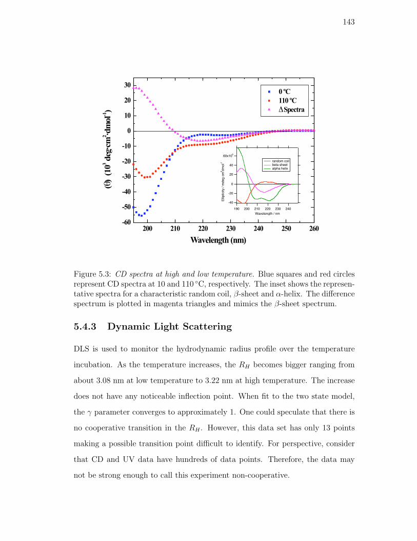
143
60x103
40
20
0
-20
-40
Ellipticity / mdeg cm2dmol-1
240230220210200190
Wavelength / nm
random coil beta sheet alpha helix
Figure 5.3: CD spectra at high and low temperature. Blue squares and red circlesrepresent CD spectra at 10 and 110 C, respectively. The inset shows the represen-tative spectra for a characteristic random coil, β-sheet and α-helix. The differencespectrum is plotted in magenta triangles and mimics the β-sheet spectrum.
5.4.3 Dynamic Light Scattering
DLS is used to monitor the hydrodynamic radius profile over the temperature
incubation. As the temperature increases, the RH becomes bigger ranging from
about 3.08 nm at low temperature to 3.22 nm at high temperature. The increase
does not have any noticeable inflection point. When fit to the two state model,
the γ parameter converges to approximately 1. One could speculate that there is
no cooperative transition in the RH . However, this data set has only 13 points
making a possible transition point difficult to identify. For perspective, consider
that CD and UV data have hundreds of data points. Therefore, the data may
not be strong enough to call this experiment non-cooperative.
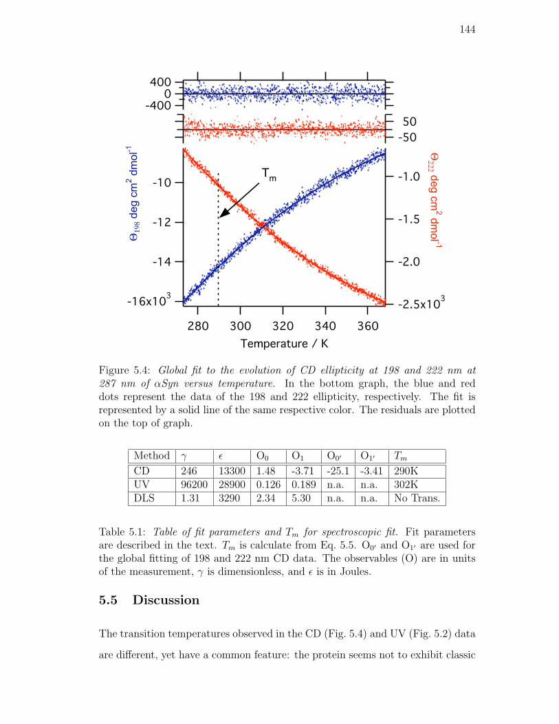
144
!!"#$ deg cm2 dmol-1 !!
%%% deg cm2 dmol -1
Tm
Figure 5.4: Global fit to the evolution of CD ellipticity at 198 and 222 nm at287 nm of αSyn versus temperature. In the bottom graph, the blue and reddots represent the data of the 198 and 222 ellipticity, respectively. The fit isrepresented by a solid line of the same respective color. The residuals are plottedon the top of graph.
Method γ ε O0 O1 O0′ O1′ Tm
CD 246 13300 1.48 -3.71 -25.1 -3.41 290KUV 96200 28900 0.126 0.189 n.a. n.a. 302KDLS 1.31 3290 2.34 5.30 n.a. n.a. No Trans.
Table 5.1: Table of fit parameters and Tm for spectroscopic fit. Fit parametersare described in the text. Tm is calculate from Eq. 5.5. O0′ and O1′ are used forthe global fitting of 198 and 222 nm CD data. The observables (O) are in unitsof the measurement, γ is dimensionless, and ε is in Joules.
5.5 Discussion
The transition temperatures observed in the CD (Fig. 5.4) and UV (Fig. 5.2) data
are different, yet have a common feature: the protein seems not to exhibit classic
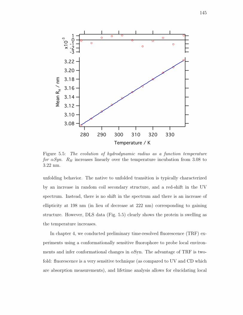
145
3.22
3.20
3.18
3.16
3.14
3.12
3.10
3.08
Mean R
H /
nm
330320310300290280
Temperature / K
-3-2-101
x10
-3
Figure 5.5: The evolution of hydrodynamic radius as a function temperaturefor αSyn. RH increases linearly over the temperature incubation from 3.08 to3.22 nm.
unfolding behavior. The native to unfolded transition is typically characterized
by an increase in random coil secondary structure, and a red-shift in the UV
spectrum. Instead, there is no shift in the spectrum and there is an increase of
ellipticity at 198 nm (in lieu of decrease at 222 nm) corresponding to gaining
structure. However, DLS data (Fig. 5.5) clearly shows the protein is swelling as
the temperature increases.
In chapter 4, we conducted preliminary time-resolved fluorescence (TRF) ex-
periments using a conformationally sensitive fluorophore to probe local environ-
ments and infer conformational changes in αSyn. The advantage of TRF is two-
fold: fluorescence is a very sensitive technique (as compared to UV and CD which
are absorption measurements), and lifetime analysis allows for elucidating local
146
environmental local states of the probe. Evaluating fluorescent lifetime distri-
butions using the same statistical mechanical formalism used in this chapter is
possible. Unfortunately, for the experiments that were conducted, there is not
enough data (five to nine temperatures) to prepare a fit and generate a Tm.
We can still inspect the lifetime evolution for trends. The transitions are
loosely consistent with those in UV and CD. In Fig. 4.5, a fast lifetime component
(designated by a the left square) appears at about 293 K for Alexa conjugated
αSyn. We speculated that this was due to a quenching mechanism resulting from
contact with the protein at higher temperature. The temperature dependence of
the NR conjugated αSyn in Fig. 4.9, shows a shift of a feature (diamonds) to a
longer lifetime with a mid-point of approximately 303 K.
Though the probes are covalently attached to the protein at the same position
(cysteine residue 19), they have significantly different properties. Alexa is fairly
hydrophilic and may prefer to spend most of its time in the solvent. At about
293K, the protein interactions with Alexa seem to increase at approximately the
same time as the increase in CD signal corresponding to an extended β-structure.
Since the protein is labeled on the N-terminal portion, this suggest there is a
conformational change occurring in this region. UV absorption changes occur at
approximately 302 K. Three of the four tyrosines are in the C-terminal region
suggesting that different parts of the protein are conformationally changing at
different temperatures.
The NR is harder to explain because its hydrophobic qualities may induce
some local collapse. The lifetime temperature trend is similar to 287 nm absorp-
tion but the connect between the two phenomenon is not known.
5.5.1 Future studies
We suspect that NMR studies of αSyn backbone may differentiate the structural
changes on a per residue basis. Theoretically, the same statistical mechanical
147
formalism can be applied such that chemical shifts for each unit in the polypep-
tide chain (N=140) has its own parameter for the lower (On0 ) and upper (On
1 )
pure observable, cooperativity (γn), and energy (εn). After each unit is fit locally,
parameters can be coupled based on their similarity. Then a global model can
be implemented with (hopefully) substantially less parameters. The global model
may point to different regions of the protein that may go under conformational
changes independently from the rest of the system, in other words, exhibit lo-
cal cooperativity. Similarly, an ensemble of structures can be generated through
computer simulations. By increasing the temperature, the ensemble of struc-
tures should change. With atomic coordinates available, converting to a physical
observable, for example RH or secondary structure propensity is trivial.
5.6 Conclusions
αSyn is a intrinsically disordered protein that has no known function. How-
ever, its primary sequence is highly conserved across species. Understanding
the monomeric conformational properties may lead to elucidating its function.
We have shown that with increasing temperature there are subtle spectroscopic
transitions present in the CD and UV data. The CD signals suggest there is a
secondary structural change occurring at a Tm of 290 K. Tyrosine absorption evo-
lution suggests a transition at 302 K and may be indicative of a conformational
change in the C-terminal region. The spectroscopic transitions are subtle and the
connection to the macroscopic thermodynamic states are speculative. However,
this type of analysis does help to formulate the hypothesis that different regions of
the protein are going through conformational changes at different temperatures.
148
References
[1] Byron Caughey and Peter T. Lansbury Jr. Protofibrils, pores, fibrils, andneurodegeneration: Separating the responsible protein aggregates from theinnocent bystanders. Annu. Rev. Neurosci., 26:267–298, 2003.
[2] Kelly A. Conway, Seung-Jae Lee, Jean-Christophe Rochet, Tomas T. Ding,Robin E. Williamson, and Peter T. Lansbury Jr. Acceleration of oligomer-ization, not fibrillization, is a shared property of both α-synuclein mutationslinked to early-onset parkinson’s disease: Implications for pathogenesis andtherapy. Proc. Nat. Acad. Sci., 97:571–576, 2000.
[3] Matthew S. Goldberg and Peter T. Lansbury Jr. Is there a cause-and-effectrelationship between α-synuclein fibrillization and parkinson?s disease? Na-ture Cell Biology, 2:E115–E119, 2000.
[4] A. Keith Dunker, J. David Lawson, Celeste J. Brown, Ryan M. Williams,Pedro Romero, Jeong S. Oh, Christopher J. Oldfield, Andrew M. Campen,Catherine M. Ratliff, Kerry W. Hipps, Juan Ausio, Mark S. Nissen, RaymondReeves, ChulHee Kang, Charles R. Kissinger, Robert W. Bailey, Michael D.Griswold, Wah Chiu, Ethan C. Garner, , and Zoran Obradovic. Intrinsicallydisordered protein. Journal of Molecular Graphics and Modelling, 19:26–59,2001.
[5] P.E. Wright and H.J. Dyson. Intrinsically unstructured proteins: re-assessingthe protein structure-function paradigm. J. Mol. Biol., 293:321–331, 1999.
[6] Akihiko Iwai, Eliezer Masliah, Makoto Yoshimoto, Nianfeng Ge, Lisa Fiana-gan, H. A. Rohan de Silva, Agnes Kittei, and Tsunao Saitoh. The precursorprotein of non-aβ component of alzheimer’s disease amyloid is a presynapticprotein of the central nervous system. Neuron, 14:467–475, 1995.
[7] Christian Lavedan. The synuclein family. Genome Research, 8:871–880,1998.
[8] Allan Chris M. Ferreon and Ashok A. Deniz. α-synuclein multistate fold-ing thermodynamics: Implications for protein misfolding and aggregation.Biochemistry, 46:4499–4509, 2007.
[9] Brigitte Nuscher, Frits Kamp, Thomas Mehnert, Sabine Odoy, ChristianHaass, Philipp J. Kahle, and Klaus Beyer. α-synuclein has a high affinityfor packing defects in a bilayer membrane. J. Bio. Chem., 279:21966–21975,2004.
149
[10] David S. Talaga, Wai Leung Lau, Heinrich Roder, Jianyong Tang, Yiwei Jia,William F. DeGrado, and Robin M. Hochstrasser. Dynamics and folding ofsingle two-stranded coiled-coil peptides studied by fluorescent energy transferconfocal microscopy. Proceedings of the National Academy of Sciences of theUnited States of America, PNAS:13021 – 13026, 2000.
[11] Alessandro Borgia, Philip M. Williams, and Jane Clarke. Single-moleculestudies of protein folding. Annu. Rev. Biochem., 77:101–125, 2008.
[12] Ashok A. Deniz, Samrat Mukhopadhyay, and Edward A. Lemke. Single-molecule biophysics: at the interface of biology, physics and chemistry. J. R.Soc. Interface, 5:15–45, 2008.
[13] Rufus Lumry, Rodney Biltonen, and John F. Brandts. Validity of the “two-state” hypothesis for conformational transitions of proteins. Biopolymers,4:917–944, 1966.
[14] Jose Nelson Onuchic, Nicholas D. Socci, Zaida Luthey-Schulten, and Peter G.Wolynes. Protein folding funnels: the nature of the transition state ensemble.Folding and Design, 1:441?450, 1996.
[15] Jack Schonbrun and Ken A. Dill. Fast protein folding kinetics. Proc. Nat.Acad. Sci., 100:12678–12682, 2003.
[16] Victor Munoz. Conformational dynamics and ensembles in protein folding.Annu. Rev. Biophys. Biomol. Struct., 36:395–412, 2007.
[17] D. B. Wetlaufer. Ultraviolet spectra of proteins and amino acids. Advan.Prot. Chem., 17:303–90, 1962.
[18] Paul H. Weinreb, Weiguo Zhen, Anna W. Poon, Kelly A. Conway, and Pe-ter T. Lansbury Jr. Nacp, a protein implicated in alzheimer’s disease andlearning, is natively unfolded. Biochemistry, 35:13709–13715, 1996.
[19] Wyn Brown, editor. Dynamic Light Scattering, The Method and Some Ap-plications. Oxford Science Publications, 1993.
[20] Jason T. Giurleo and David S. Talaga. Global fitting without a global model:Regularization based on the continuity of the evolution of parameter distri-butions. The Journal of Chemical Physics, 128:114114–(1–18), 2008.
[21] David R. Lide, editor. CRC Handbook of Chemistry and Physics, 88th Edi-tion (Internet Version 2008). RC Press/Taylor and Francis, Boca Raton,FL, 2008.
[22] Harold Edelhoch. Spectroscopic determination of tryptophan and tyrosinein proteins. Biochemistry, 6:1948–1954, 1967.
150
[23] Pierre Nicolas, Thomas A. Bewley, Laszlo Graf, and Choh Hao Li. β-endorphin: Demonstration of a tertiary structure in aqueous solution. Proc.Nat. Acad. Sci. USA, 78:7290–7293, 1981.
[24] Kunihiko Gekkof and Serge N. Timasheff. Thermodynamic and kinetic ex-amination of protein stabilization by glycerol. Biochemistry, 20:4677–4686,1981.
[25] N. Greenfield, B. Davidson, and G. D. Fasman. The use of computed op-tical rotatory dispersion curves for the evaluation of protein conformation.Biochemistry, 6:1630–1637, 1967.
[26] N. Greenfield and G. D. Fasman. Computed circular dichroism spectra forthe evaluation of protein conformation. Biochemistry, 8:4108–4116, 1969.
151
Chapter 6
Aggregation methods of α-synuclein.
6.1 Summary
Proposed aggregation mechanisms of α-synuclein fit a sigmoidal model of in vitro
amyloid formation. This includes lag, growth and elongation phase. The phases
are usually explained via nucleation mechanism. We show that differences in
sample preparation and aggregation conditions change self-assembly rates and
suspect that the balance of critical intermediate species are shifted. We have found
that methods typically used for investigation of amyloid formation in vitro involve
incomplete filtering and vigorous shaking. We suggest several other experiments
that can be done to elucidate the intermediate species in a more controlled way.
6.2 Introduction
Mechanism and amyloid formation.
The dogma surrounding the mechanism of amyloid formation is rooted in the
observations of sigmoidal fibril growth in vitro. 6.1 The kinetics are described in
three main phases:
1. a lag phase, in which monomers conformationally convert to nuclei exhibit-
ing the typical amyloid cross-β structure. This continues until a critical
concentration of nuclei is reached, marking the beginning of the
2. growth phase. During this phase, nuclei quickly grow into protofilaments
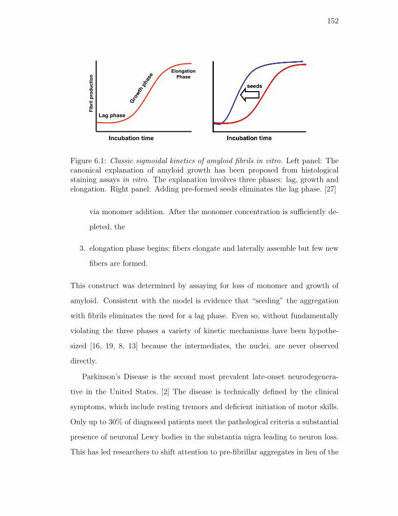
152
Incubation time (days)
Monomer loss
seeds
Incubation time (days)
Monomer loss
Lag phase
Growth phase Mature
phase
Fibril production
Elongation
Phase
Figure 6.1: Classic sigmoidal kinetics of amyloid fibrils in vitro. Left panel: Thecanonical explanation of amyloid growth has been proposed from histologicalstaining assays in vitro. The explanation involves three phases: lag, growth andelongation. Right panel: Adding pre-formed seeds eliminates the lag phase. [27]
via monomer addition. After the monomer concentration is sufficiently de-
pleted, the
3. elongation phase begins; fibers elongate and laterally assemble but few new
fibers are formed.
This construct was determined by assaying for loss of monomer and growth of
amyloid. Consistent with the model is evidence that “seeding” the aggregation
with fibrils eliminates the need for a lag phase. Even so, without fundamentally
violating the three phases a variety of kinetic mechanisms have been hypothe-
sized [16, 19, 8, 13] because the intermediates, the nuclei, are never observed
directly.
Parkinson’s Disease is the second most prevalent late-onset neurodegenera-
tive in the United States. [2] The disease is technically defined by the clinical
symptoms, which include resting tremors and deficient initiation of motor skills.
Only up to 30% of diagnosed patients meet the pathological criteria a substantial
presence of neuronal Lewy bodies in the substantia nigra leading to neuron loss.
This has led researchers to shift attention to pre-fibrillar aggregates in lieu of the
153
fibrils themselves. Understanding the nuances of the true mechanism (i.e. identi-
fying intermediate species) may have direct relevance to the development of the
effective preventative therapeutic agents. [22, 24, 7]
Incubation conditions affect aggregation rates.
α-Synuclein (αSN) is the major fibrillar component of Lewy bodies. [3, 2] Table
6.2 is a select list of publications that have investigated αSN amyloid forma-
tion properties. The preparation of monomeric protein and incubation conditions
(i.e. shaking, stirring, quiescent, etc.) have the largest effect on aggregation
rates. Having pure monomeric protein at the start of any incubation is critical.
Remember, the canonical explanation of amyloid formation involves the notion
that reseeding eliminates the lag phase. Incubation conditions are also very im-
portant since it was shown nearly 80 years ago that shaking promotes protein
aggregation.[21]. Stirring with Teflon stir bars has also been shown to increase
aggregation rates, even when the headspace has been eliminated. [23]
As shown in Table 6.2, starting and incubation conditions are critical factors
for the rate of amyloid formation. Not only must these have to be considered dur-
ing experimental design but also when considering potential mechanisms. In fact
ignoring these effects may lead to a gross misunderstanding of the experimental
observations.
Experimental design
In this chapter, we investigate six possible starting and three different aggregation
conditions in order to (1) establish an appropriate protocol for generating αSN
fibrils, (2) investigate and explain any differences in timescales of amyloid forma-
tion due to starting and aggregation conditions, and (3) design future meaningful
experiments.
Native gel electrophoresis is utilized to investigate the content of the starting
154
material prepared for two different methods typically found in the literature of
preparing the αSN. A fluorescent stain adds several orders of magnitude sensi-
tivity as compared to visible stains in order to more easily identify aggregates.
Method 1 dissolves lyophilized αSN in an unbuffered strong base, then neutral-
izes with strong acid, followed by centrifuging to remove insoluble aggregates.
Method 2 reconstitutes lyophilized protein in buffer directly, passed through a
100 kDa molecular weight cutoff (MWCO) filter to remove insoluble material.
Method 3 is a variation of Method 1 but not used for the incubation studies.
This method utilizes buffered basic and acidic conditions to dissolve aggregates
as a way to keep the protein from being exposed to extreme pH conditions and
to potentially have increased reproducibility of the method.
The four starting/incubation conditions studied are:
1. Method 1 (100 kDa MWCO filtering) / shaking or FS
2. Method 3 (base dissolving, centrifuge) / shaking or US
3. Method 3 (base dissolving, centrifuge) / rotating or UR
A fourth unfiltered, quiescent experiment is also conducted as a control. It was
monitored only with light scattering because its gestation time was expected to
be much longer than its agitated counterparts.
The presence of amyloid is assayed using steady-state thioflavinT lumines-
cence (SS), static light scattering (SLS) and atomic force microscopy (AFM).
ThioflavinT (ThT) gains a new excitation band at 450 nm when dimers (or more)
couple in a structured environment. ThT luminescence is often used to assay for
amyloid cross-β structure. Atomic force microscope images were taken to con-
firm the presence of amyloid fibrils at the conclusion of experiment. Though not
a specific test for amyloid, SLS can be a useful tool for reporting the change of
the size of scatters in solution. As the solute aggregates, the scattering intensity
will increase.
155
Time-resolved fluorescence (TRF) and dynamic light scattering (DLS) are two
methods utilized to gain more specific information about species in solution along
the incubation time course. DLS has been used extensively to monitor protein
aggregation [15, 17] and will be used primarily to track the early aggregation
stages. ThT lifetime measurements are useful in elucidating different types of
binding modes or aggregate species along the amyloid formation pathway. [5] The
GIPG procedure [6] was used to fit the evolution of the lifetime and particle size
distributions over the time course for the TRF and DLS, respectively.
6.3 Methods
Chemicals
ThT, aminopropyltriethoxysilane (APTES), and dibasic and monobasic sodium
phosphate were purchased from Sigma.
Protein Preparation
Escherichia coli BL21 DE3 strain (Invitrogen Inc.) were transfected by plasmids
(pT7-7) encoded human αSN A19C mutant and were gifts from Professor Jean
Baum (Rutgers University, Piscataway, NJ). Expression and purification of mu-
tant αSN followed published protocols. [25]
Sample preparation for time-zero Native Gel
Three primary methods were used to compare different preparation methods for
αSN:
Method 1 was adopted from Ref. [18] by the best of our abilities. 1 mg
of lyophilized αSN was reconsitutied in 10 µL of Millipore water with 3 µL of
0.1 N NaOH at room temperature to dissolve insoluble aggregate species. After
20 minutes, 3 µL of 0.1 N HCl was then added to lower the pH. 894 µL of 10mM
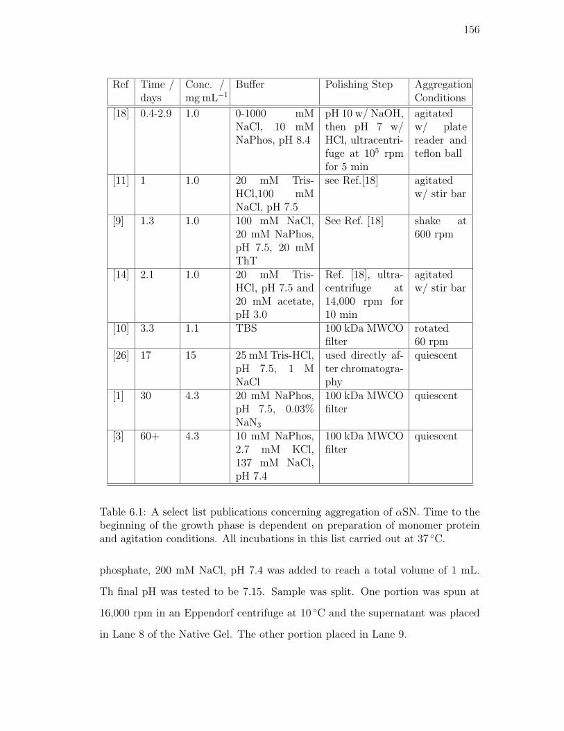
156
Ref Time /days
Conc. /mg mL−1
Buffer Polishing Step AggregationConditions
[18] 0.4-2.9 1.0 0-1000 mMNaCl, 10 mMNaPhos, pH 8.4
pH 10 w/ NaOH,then pH 7 w/HCl, ultracentri-fuge at 105 rpmfor 5 min
agitatedw/ platereader andteflon ball
[11] 1 1.0 20 mM Tris-HCl,100 mMNaCl, pH 7.5
see Ref.[18] agitatedw/ stir bar
[9] 1.3 1.0 100 mM NaCl,20 mM NaPhos,pH 7.5, 20 mMThT
See Ref. [18] shake at600 rpm
[14] 2.1 1.0 20 mM Tris-HCl, pH 7.5 and20 mM acetate,pH 3.0
Ref. [18], ultra-centrifuge at14,000 rpm for10 min
agitatedw/ stir bar
[10] 3.3 1.1 TBS 100 kDa MWCOfilter
rotated60 rpm
[26] 17 15 25 mM Tris-HCl,pH 7.5, 1 MNaCl
used directly af-ter chromatogra-phy
quiescent
[1] 30 4.3 20 mM NaPhos,pH 7.5, 0.03%NaN3
100 kDa MWCOfilter
quiescent
[3] 60+ 4.3 10 mM NaPhos,2.7 mM KCl,137 mM NaCl,pH 7.4
100 kDa MWCOfilter
quiescent
Table 6.1: A select list publications concerning aggregation of αSN. Time to thebeginning of the growth phase is dependent on preparation of monomer proteinand agitation conditions. All incubations in this list carried out at 37 C.
phosphate, 200 mM NaCl, pH 7.4 was added to reach a total volume of 1 mL.
Th final pH was tested to be 7.15. Sample was split. One portion was spun at
16,000 rpm in an Eppendorf centrifuge at 10 C and the supernatant was placed
in Lane 8 of the Native Gel. The other portion placed in Lane 9.

157
Method 2 replaces the base dissolving step with reconstituting protein di-
rectly into 10 mM phosphate, 200 mM NaCl, pH 7.4 buffer then passed through a
100 kDa MWCO Microcon centrifuge filter from Millipore. The filtrate was placed
in lane 3, while the retentate was placed in lane 4. Similarly, sample passed via a
30 kDa filter was placed in lane 5 and the retentate in lane 6. Unfiltered samples
were placed in lanes 2 and 3.
Method 3 dissolves the lyophilized protein in a basic buffer. 6.5 mg of αSN
was dissolved in 1 mM Na3PO4 at pH 11 for 20 minutes at room temperature.
116 µL of 0.5M phosphate buffer at pH 6.8 was utilized to bring the pH back
down. After 1mL of 1.2M NaCl was added, the concentration of the protein was
determined to be 1.77 mg/mL using an extinction coefficient αSN of 0.4 mg cm2.
Millipore water was added to a final concentration of 1 mg/mL. Sample was
centrifuged as above and placed in Lane 7.
Sample preparation for incubation
Samples were prepared labeled UR, US, FS, for unfiltered-rotated, unfiltered-
shaken, filtered-shaken, respectively. US and UR were prepared by Method 1
using 1.2 mL of the stock 1.0 mg/mL αSN in matched type-47 semi-micro quartz
cuvettes with screw cap from NSG Precision Cells Inc. (Farmingdale, NY). FS
was prepared by Method 2 and added to the cuvette. Samples were incubated
in the presence ThT as in Ref. [18]. 6 µL of 1 mM ThT was added making a final
concentration of 5 µM. All samples were very gently mixed prior to incubation.
There was about 1.7 mL of headspace in each cuvette. UQ was prepared by
reconstituting Method 2 but was not filtered. Only SLS was measured on this
sample.
A homemade shaker tray was built for these experiments and made from a
Styrofoam cuvette holder attached to a FISHERbrand Vortex Genie 2 (model
2-812). The tray was oriented such that two cuvettes laid flat with the wider
158
inner dimension parallel to the plane of the floor. The shaking rate was measured
to be about 590 rpm. For the rotated sample, the cuvette was secured on ”Roto-
Torque” (model 7637) wheel rotator at 47 rpm. Samples were agitated at 37 C.
Every 45 to 60 minutes, a sample was removed and measurements were taken in
a quiescent condition. The total incubation (including measurement time) was
nearly 20 hours long.
ThioflavinT assay
SS measurements of ThT luminescence was made using a Cary with a Peltier
heating unit. Excitation was 450 nm with a 5 nm slit. Emission was observed
from 462 to 650 nm at a rate of 300 nm per minute with a 5 nm slit.
TRF measurements were acquired by time-correlated single-photon counting
with a setup previously described [5]. In order to monitor laser stability during
a particular incubation time point, ten separate data transients were taken, each
for 30 seconds. After ensuring that time-zero populations for each data trace were
consistent, the data was added together. Peak intensity ranged from several hun-
dred counts at the beginning of the incubation to over 100,000 by the timecourse
completion.
ThT lifetime distributions were globally fit using GIPG [6] on a 60-point
grid, logarithmically-spaced in lifetime ranging from 0.01 to 10 ns. GIPG only
assumes that there is a smooth transition of fit parameters (in this case, the in-
verse Laplace transform of a instrument-response-convoluted exponentials) along
the experimental coordinate. Over the course of 20 hours of incubation time,
laser fluctuations may corrupt this continuity condition. Therefore a correc-
tion factor was applied to the overall intensity of the transients based on the
SS ThT intensity measurements because they have a more reliable and consistent
power source. This was done by first completing an Active-Set fit on the unper-
turbed data. [6, 12] The GIPG algorithm was originally set up to fit TCSPC on
159
a population-weighted basis, but the parameters can intensity-weighted by mul-
tiplying the amplitude of a parameter by its corresponding lifetime. A correction
factor was created by comparing the sum of the intensity-weighted parameters for
a particular incubation time (not considering the scattering or baseline terms) to
the total sum intensity of the steady-state emission between 478 to 487 nm (cor-
responding to the slit width used for the lifetime measurement). A multiplicative
correction factor was applied to the TCSPC data for each transient and the error
was propagated accordingly. The data was fit using 200,000 iterations with a step
parameter of 0.9. Probability-to-reject (as compared to the Active-Set fit) was
always less than 0.05.
DLS and SLS assay
DLS experimental setup and cleaning procedure has been described previously [5],
with the exception that the samples were contained in reduced volume cuvettes.
Three correlation functions were obtained per sample, per incubation time for
30 seconds at 37 C. Data was averaged and error was propagated accordingly.
On occasion, correlation functions were discontinuous and were discarded. This
occurred most with the unfiltered samples, especially at late incubation times.
Scattering count rates (SLS) were simultaneously recorded with correlation func-
tions.
Data was fit using the GIPG method on a 91-point, logarithmically-spaced
grid containing seven decades of decay time from 0.0001 to 100 ms. The first and
last decades each had five points, whereas the remaining contained twenty decay
times per decade. Third derivative regularizer was implemented and all fits had
a probability-to-reject of less than 0.01 as compared to an Active Set fit. 100,000
iterations and a step parameter of 0.9 were used.
Decay time was converted to hydrodynamic radius as shown in Ref. [5]. The
viscosity of the buffer solution, η0, at 37 C was 0.7345, measured by VISCOlabs
160
4100 viscometer. The refractive index of the buffer was taken to be 1.334. The
characteristic density of the αSN determined from assignment of a temperature
titration DLS experiment in chapter 5 was used to scale the oligomer sizes by
RH,monomerN1/3, where N is monomers per aggregate.
AFM
Preparation and execution of AFM measurements have been previously described
in Ref. [5]. AFM was taken at the conclusion of the experiment.
Native gel electrophoresis
A precasted Novex Tris Glycine Native gel was run via the Invitrogen protocol.
NativeMark Unstained Protein Standard was used as the marker. The gel was
stained with the fluorescent SYPRO Ruby Protein Stain (BIORAD).
Photograph of final product
A photograph was taken at the completion of the incubation with a Samsung
Flipshot (SCH-U900) cellular phone.
6.4 Results
6.4.1 Initial conditions
Native gel electrophoresis reveals the differences in preparation procedures. 6.2
The monomer band sits just below the 146 kDa molecular weight marker. In
contrast to the standards, αSN is not a globular protein. In fact the hydrodynamic
radius of αSN is more similar to the characteristic radius of human insulin protein,
molecular weight of 65 kDa. Filtering with a 100 kDa filter may remove particles
as small as αSN dimers and certainly tetramers.
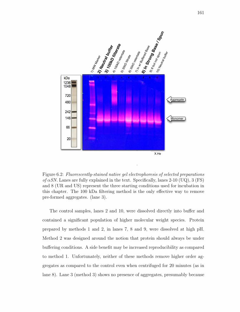
161
2) Neutral buffer
10) Neutral buffer
3) 100kD filterate
5) 30kD filtrate
4) 100kD retentate
6) 30kD retentate
9) 8 but not spun
8) In Strong Base / Spun
7) In w/ Buffered Base
1) MW Marker
X.He
Aggregate
Monomer
Figure 6.2: Fluorescently-stained native gel electrophoresis of selected preparationsof αSN. Lanes are fully explained in the text. Specifically, lanes 2-10 (UQ), 3 (FS)and 8 (UR and US) represent the three starting conditions used for incubation inthis chapter. The 100 kDa filtering method is the only effective way to removepre-formed aggregates. (lane 3).
The control samples, lanes 2 and 10, were dissolved directly into buffer and
contained a significant population of higher molecular weight species. Protein
prepared by methods 1 and 2, in lanes 7, 8 and 9, were dissolved at high pH.
Method 2 was designed around the notion that protein should always be under
buffering conditions. A side benefit may be increased reproducibility as compared
to method 1. Unfortunately, neither of these methods remove higher order ag-
gregates as compared to the control even when centrifuged for 20 minutes (as in
lane 8). Lane 3 (method 3) shows no presence of aggregates, presumably because
162
100 kDa filter removed them. It is apparent from the 100 kDa retentate in lane
4 that aggregates are present in the unfiltered samples. As a final test, a 30 kDa
filter was implemented in lanes 5 and 6, but the results were puzzling. Lane
5 is the filtered solution but looks similar to the unfiltered control, but less in-
tense. Though the retentate in lane 6 has aggregate species, there is a significant
monomer contribution.
6.4.2 Final product - Visual Inspection and AFM
Visually inspecting the samples at the completion of the experiment is a reality
check for the spectroscopic measurements and is shown in Fig. 6.4. All samples
exhibited bubbles filling the headspace. Both FS and US have a similar bubble size
and density as compared to UR. Crudely estimating, there are 3 larger bubbles
and 5 smaller bubbles that stretch across the 1 cm width of the cuvette for UR
and US, respectively.
US had a yellow “milky” color with fine suspended particulates. UR had a
yellow tint, but also had large particulates that were prone to settle to the bottom
of the cuvette. Conversely, the FS sample was clear and had a slight yellow hue
similar to that of a stock 5µM stock solution of ThT.
AFM images in Fig. 6.3 were taken to ensure amyloid fibrils were being gen-
erated. The results were consistent with the visual inspection of the sample after
the conclusion of the experiment. Several AFM images of the FS sample were
taken; fibrils were a rare find. This may be expected since the sigmoidal pattern
of static light scattering and ThT luminescence was not observed for this sample.
Furthermore, the sample was still clear to the eye by the time the AFM sample
was prepared.
On the other hand, US was hazy visually and the corresponding AFM image
exhibited a fairly dense fibril network across the entire modified mica surface.
This suggests that if fibril species do exist they will adhere to the surface. Proper
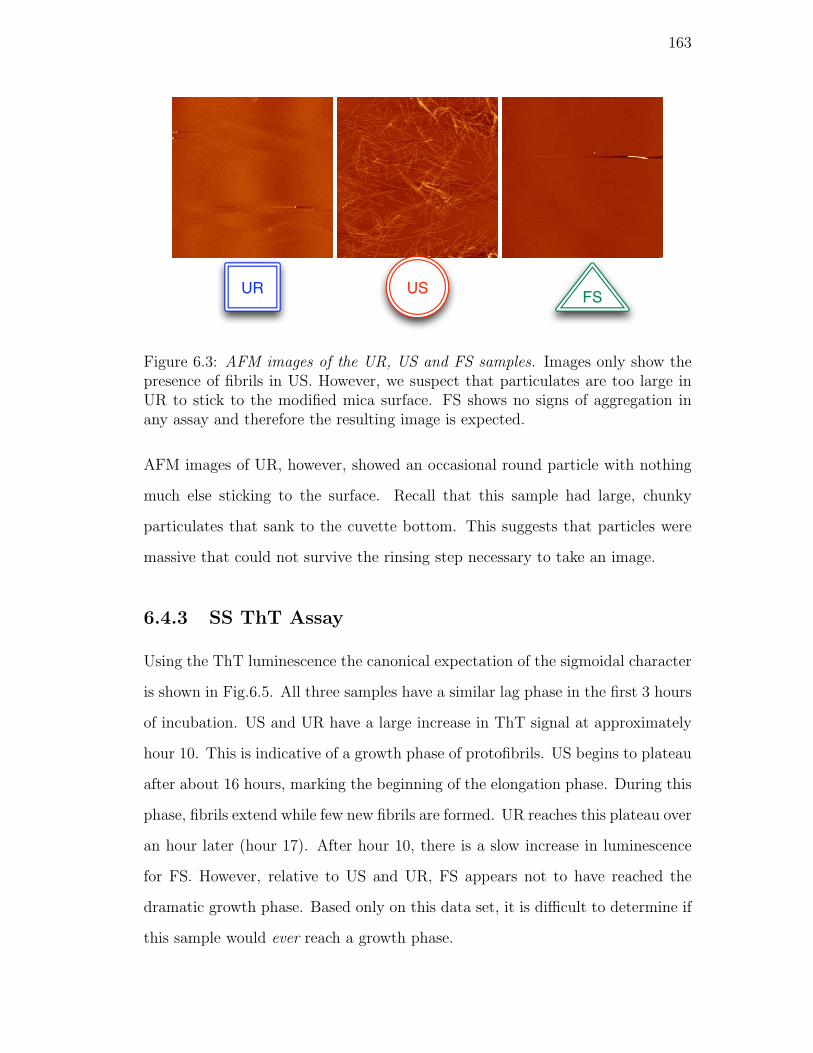
163
UR USFS
Figure 6.3: AFM images of the UR, US and FS samples. Images only show thepresence of fibrils in US. However, we suspect that particulates are too large inUR to stick to the modified mica surface. FS shows no signs of aggregation inany assay and therefore the resulting image is expected.
AFM images of UR, however, showed an occasional round particle with nothing
much else sticking to the surface. Recall that this sample had large, chunky
particulates that sank to the cuvette bottom. This suggests that particles were
massive that could not survive the rinsing step necessary to take an image.
6.4.3 SS ThT Assay
Using the ThT luminescence the canonical expectation of the sigmoidal character
is shown in Fig.6.5. All three samples have a similar lag phase in the first 3 hours
of incubation. US and UR have a large increase in ThT signal at approximately
hour 10. This is indicative of a growth phase of protofibrils. US begins to plateau
after about 16 hours, marking the beginning of the elongation phase. During this
phase, fibrils extend while few new fibrils are formed. UR reaches this plateau over
an hour later (hour 17). After hour 10, there is a slow increase in luminescence
for FS. However, relative to US and UR, FS appears not to have reached the
dramatic growth phase. Based only on this data set, it is difficult to determine if
this sample would ever reach a growth phase.
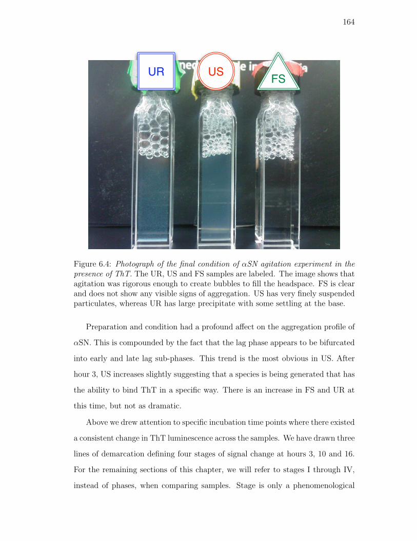
164
UR USFS
Figure 6.4: Photograph of the final condition of αSN agitation experiment in thepresence of ThT. The UR, US and FS samples are labeled. The image shows thatagitation was rigorous enough to create bubbles to fill the headspace. FS is clearand does not show any visible signs of aggregation. US has very finely suspendedparticulates, whereas UR has large precipitate with some settling at the base.
Preparation and condition had a profound affect on the aggregation profile of
αSN. This is compounded by the fact that the lag phase appears to be bifurcated
into early and late lag sub-phases. This trend is the most obvious in US. After
hour 3, US increases slightly suggesting that a species is being generated that has
the ability to bind ThT in a specific way. There is an increase in FS and UR at
this time, but not as dramatic.
Above we drew attention to specific incubation time points where there existed
a consistent change in ThT luminescence across the samples. We have drawn three
lines of demarcation defining four stages of signal change at hours 3, 10 and 16.
For the remaining sections of this chapter, we will refer to stages I through IV,
instead of phases, when comparing samples. Stage is only a phenomenological
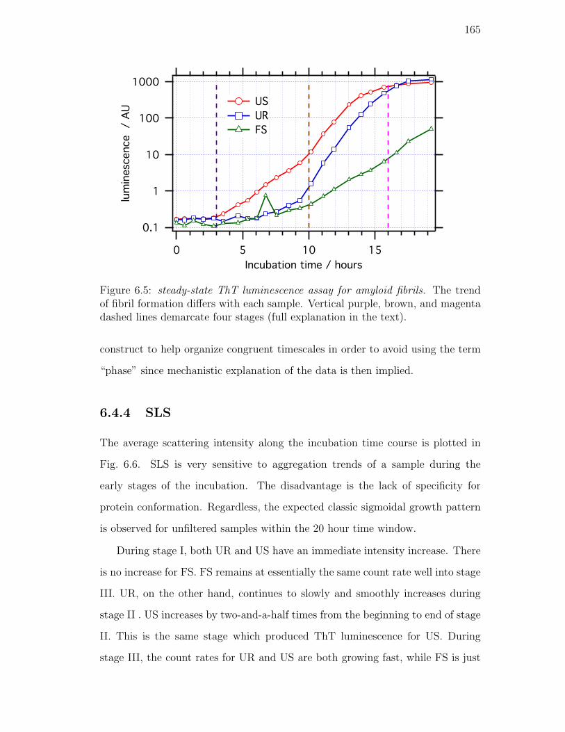
165
0.1
1
10
100
1000
lum
inesc
ence / A
U
151050
Incubation time / hours
US
UR
FS
Figure 6.5: steady-state ThT luminescence assay for amyloid fibrils. The trendof fibril formation differs with each sample. Vertical purple, brown, and magentadashed lines demarcate four stages (full explanation in the text).
construct to help organize congruent timescales in order to avoid using the term
“phase” since mechanistic explanation of the data is then implied.
6.4.4 SLS
The average scattering intensity along the incubation time course is plotted in
Fig. 6.6. SLS is very sensitive to aggregation trends of a sample during the
early stages of the incubation. The disadvantage is the lack of specificity for
protein conformation. Regardless, the expected classic sigmoidal growth pattern
is observed for unfiltered samples within the 20 hour time window.
During stage I, both UR and US have an immediate intensity increase. There
is no increase for FS. FS remains at essentially the same count rate well into stage
III. UR, on the other hand, continues to slowly and smoothly increases during
stage II . US increases by two-and-a-half times from the beginning to end of stage
II. This is the same stage which produced ThT luminescence for US. During
stage III, the count rates for UR and US are both growing fast, while FS is just
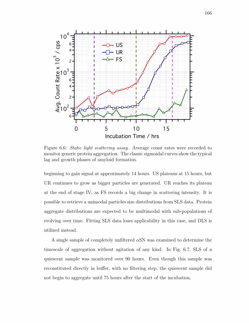
166
6
102
2
4
6
103
2
4
6
104
Avg. Count
Rate
x 1
03 /
cps
151050
Incubation Time / hrs
US
UR
FS
Figure 6.6: Static light scattering assay. Average count rates were recorded tomonitor generic protein aggregation. The classic sigmoidal curves show the typicallag and growth phases of amyloid formation.
beginning to gain signal at approximately 14 hours. US plateaus at 15 hours, but
UR continues to grow as bigger particles are generated. UR reaches its plateau
at the end of stage IV, as FS records a big change in scattering intensity. It is
possible to retrieve a unimodal particles size distributions from SLS data. Protein
aggregate distributions are expected to be multimodal with sub-populations of
evolving over time. Fitting SLS data loses applicability in this case, and DLS is
utilized instead.
A single sample of completely unfiltered αSN was examined to determine the
timescale of aggregation without agitation of any kind. In Fig. 6.7, SLS of a
quiescent sample was monitored over 90 hours. Even though this sample was
reconstituted directly in buffer, with no filtering step, the quiescent sample did
not begin to aggregate until 75 hours after the start of the incubation.
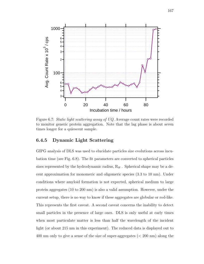
167
3
4
56
100
2
3
4
56
1000
Avg
. Cou
nt R
ate
x 10
3 / cp
s
806040200Incubation time / hours
Figure 6.7: Static light scattering assay of UQ. Average count rates were recordedto monitor generic protein aggregation. Note that the lag phase is about seventimes longer for a quiescent sample.
6.4.5 Dynamic Light Scattering
GIPG analysis of DLS was used to elucidate particles size evolutions across incu-
bation time (see Fig. 6.8). The fit parameters are converted to spherical particles
sizes represented by the hydrodynamic radius, RH . Spherical shape may be a de-
cent approximation for monomeric and oligomeric species (3.3 to 10 nm). Under
conditions where amyloid formation is not expected, spherical medium to large
protein aggregates (10 to 200 nm) is also a valid assumption. However, under the
current setup, there is no way to know if these aggregates are globular or rod-like.
This represents the first caveat. A second caveat concerns the inability to detect
small particles in the presence of large ones. DLS is only useful at early times
when most particulate matter is less than half the wavelength of the incident
light (or about 215 nm in this experiment). The reduced data is displayed out to
400 nm only to give a sense of the size of super-aggregates (< 200 nm) along the
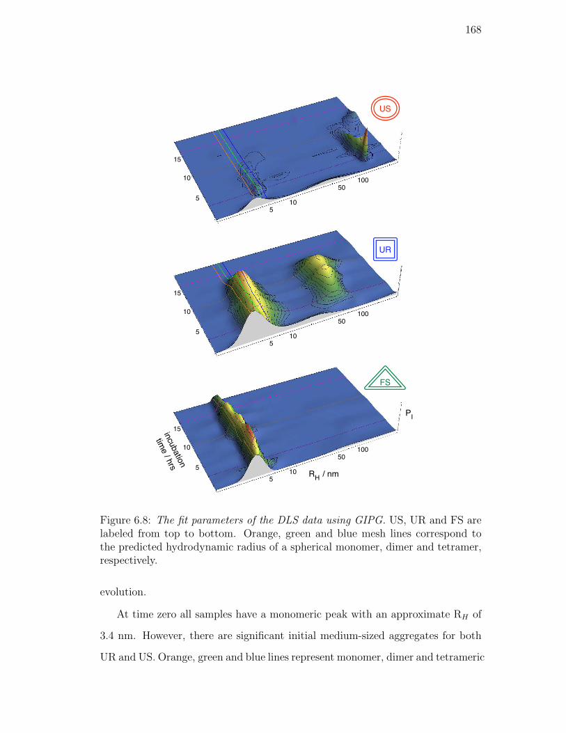
168
15
10
5
50
10
5
100
incubation
time / hrs
PI
RH / nm
15
10
5
50
10
5
100
15
10
5
50
10
5
100
FS
UR
US
Figure 6.8: The fit parameters of the DLS data using GIPG. US, UR and FS arelabeled from top to bottom. Orange, green and blue mesh lines correspond tothe predicted hydrodynamic radius of a spherical monomer, dimer and tetramer,respectively.
evolution.
At time zero all samples have a monomeric peak with an approximate RH of
3.4 nm. However, there are significant initial medium-sized aggregates for both
UR and US. Orange, green and blue lines represent monomer, dimer and tetrameric
169
species by scaling the monomer unit by constant density. Even though UR and
US were prepared in identical fashion, US has slightly larger and greater concen-
tration of initial aggregates. FS does not have any aggregates. The time-zero
aggregates were consistent with native gel.
As stage I progresses, there is immediate oligomerization in all samples. UR
has a wide particle size distribution for the oligomeric species with a mean about
the same as a tetramer. Also, the initial medium-sized aggregates have grown to
large (70 nm) species. This distribution is wide suggesting a range of particles
sizes. DLS data was corrupted during hours 1 and 2 for US and were not used in
the analysis. We cannot comment on the evolution during this stage. There are
no aggregates formed in FS as measured by DLS. In this sample, the monomer
oligomerized to form a narrow distribution of dimeric species.
At the start of stage II, fairly monodisperse, large (180 nm) aggregates domi-
nate the intensity signal in the US. US also self-associates monomers into narrow
distribution of sizes consistent with a trimer. This peak slowly decreases and shifts
to large oligomers by the conclusion of stage II. In terms of large aggregates, in
the US sample there is steady decrease, whereas UR slowly gain population. FS
does not have any detectable aggregates present. Keep in mind, the parameters
represented in Fig. 6.8 are intensity-weighted and do not reflect number of par-
ticles in solution. Converting intensity-weighted parameters to number-weighted
parameters reveal that the large aggregates are seven to eight orders of magnitude
less in number than the time-zero monomer population. This would be consis-
tent with the notion that metastable species present in the amyloid formation
mechanism are short lived (or low population).
For UR and US, stage III represents the approximate time of the growth
phase where there are significant increases in scattering and ThT luminescence.
By the start of stage III, there are super-aggregates (approximately 300 nm) being
generated in US. The disappearance of the oligomeric and large aggregates may
170
be due to the presence of super-aggregates swamping the signal and not due to the
complete conversion of these species. Similarly, oligomeric and aggregate species
in the UR sample are overwhelmed by super-aggregates after hour 12.
FS does not change much until the end of stage III. At this point, there is a
slow decrease in signal coinciding with an increase in static light scattering (see
Fig. 6.6). Without any evidence of intermediate aggregate particles present by
DLS, the aggregation is most likely due to super-aggregates.
6.4.6 Time-Resolved ThT luminescence
The time-resolved fluorescence resolves details concerning binding environments
of the intercalated fluorophore. ThT lifetimes evolve across the incubation time-
course as species begin to bind ThT in a luminescence-competent way. At the
beginning of the incubation little binding of ThT is observed.
The final incubation time is useful to characterize first because there is pre-
sumably fibril-bound ThT. At the conclusion of the UR and US incubation, a
plateau of ThT luminescence is reached (see Fig. 6.5). 95.6% of the final intensity-
weighted lifetime distribution of UR is represented by a 2.0-ns species. Most of
the remaining intensity is from a shorter 660-ps species (3.6%) and longer 5.0-ns
(0.58%) species. The US sample has the same 2.0-ns species but has slightly less
of the majority at 93.6%. Conversely, there is small increase in the intensity of
the 640 ps component to 5.7%. Also, there is a small contribution (0.28%) of a
170 ps component which is not present in the UR sample. The longest lifetime
component is shifted to about 6.3 ns and represents 0.20% of the intensity. In
contrast, FS has not reached a plateau in SLS or SSF by 19 hours. This is re-
flected by a different lifetime distribution, centered at 1.6 ns (93.0%) and 660 ps
(5.9%).
At the beginning of stage III, US exhibits a 1.4-ns feature. This feature shifts
slowly to 1.6 ns by the middle of this stage, as shorter 660 ps feature appears.
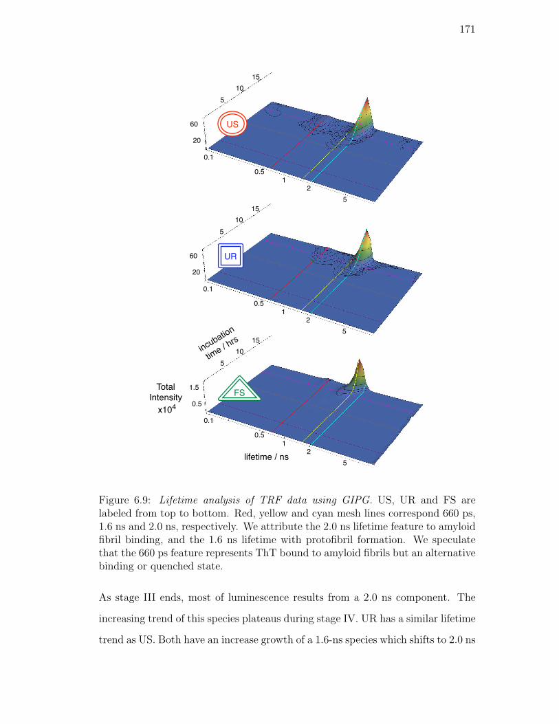
171
10
5
15
60
20
0.1
12
5
0.5
10
5
15
60
20
0.1
12
5
0.5
lifetime / ns
10
5
15
1.5
0.5
0.1
12
5
0.5
incubation
time / hrs
Total
Intensity
x104
UR
US
FS
Figure 6.9: Lifetime analysis of TRF data using GIPG. US, UR and FS arelabeled from top to bottom. Red, yellow and cyan mesh lines correspond 660 ps,1.6 ns and 2.0 ns, respectively. We attribute the 2.0 ns lifetime feature to amyloidfibril binding, and the 1.6 ns lifetime with protofibril formation. We speculatethat the 660 ps feature represents ThT bound to amyloid fibrils but an alternativebinding or quenched state.
As stage III ends, most of luminescence results from a 2.0 ns component. The
increasing trend of this species plateaus during stage IV. UR has a similar lifetime
trend as US. Both have an increase growth of a 1.6-ns species which shifts to 2.0 ns
172
later in the stage. However, UR does not have a 1.4-ns feature.
The small ThT SS intensity present at the end of stage III in FS (see Fig. 6.5)
is due to a short 1.2-ns lifetime. The lifetime shifts during stage IV to 1.6 ns.
This lifetime has preceded the growth of a 2.0-ns species that was present at the
end of the growth phase in UR and US. The added lifetime information suggests
that FS is on pathway to form amyloid fibrils.
6.4.7 Data recapitulation
FS
Filtering reconstituted αSN with a 100 kDa MWCO filter left only monomeric
species shown by native gel (Fig. 6.2) and time-zero DLS (Fig. 6.8). Particle size
distribution evolution measured by DLS showed an initial dimerization within
stage I, but no significant increase in SLS signal was reported (Fig. 6.6). In
fact a significant scattering trend did not occur until the middle of stage III.
However, ThT luminescence (Fig. 6.5) increased from stage II through stage IV,
without the sharp growth phase as shown by UR and US. The majority lifetime
responsible for this increase starts at approximately 1.2 ns and shifts to 1.6 ns.
The 1.6 ns feature was shown by both UR and US during the stage III, or the
growth phase. AFM images (Fig. 6.3) do not show any fibril structures attached
to the modified mica surface and, upon visual examination (Fig. 6.4), the sample
was clear without particulates present.
US
Native gel and time-zero DLS showed presence of aggregate species at the start
of the experiment. During the stage I, a narrow distribution of oligomeric species
were created from self-associating monomers. At the end of stage I, there was a
significant increase in scattering signal as shown by SLS. Interpretation of DLS
173
suggests that the increase of SLS signal was most likely due to large, narrowly
distributed particles converted from the presence of time-zero aggregates.
No ThT signal was demonstrated until the beginning of stage II. During stage
II there was a modest ThT and SLS increase, while presence of large aggregates
disappeared, suggesting a conversion to super-aggegrates. ThT and SLS signal
increased at a greater rate at the beginning of stage III and was attributed to a
growth phase. ThT lifetime distributions shifted from 1.4 to 1.6 ns, then to 2.0 ns
by the conclusion of stage III. This may suggest the conversion of protofibril to
amyloid fibril structures. Alternative binding orientations may be responsible for
shorter lifetime components of approximately 650 ns.
By stage IV the SLS and ThT intensity plateaued as shown in Fig. 6.5. The
intensity trend is indicative of a slower rate to the creation of new aggregates;
the 2.0 ns lifetime implies the aggregates are amyloid fibrils. The argument is
strengthened by AFM imaging (Fig. 6.3). Amyloid fibrils stuck to the surface
and demonstrated a network of fibrillar structures and was consistent with the
final solution of small suspended particulates. (Fig. 6.4).
UR
As in US, native gel and time-zero DLS showed presence of aggregate species at
the start of the experiment. During the stage I, self-associating monomers created
a large distribution of oligomeric species. At the same time, a wide distribution
of aggregates were converted from the initial aggregate left after reconstitution.
At the end of stage I, there was a slight increase in scattering signal as shown by
SLS in Fig. 6.6. Interpretation of DLS suggests that contrary to shaking, rotating
does not create a significant population of super-aggregates early on.
Little ThT or SLS signal was demonstrated until the end of stage II at which
there was a dramatic change. ThT and SLS signal increased at a greater rate at
the beginning of stage III and was attributed to a growth phase. ThT lifetime
174
distributions shifted from 1.6 to 2.0 ns by the conclusion of this stage. The 1.4-ns
feature was not present in UR.
By the end of stage IV, the SLS and ThT intensity plateaued. As in US, the
2.0 ns lifetime suggests the aggregates are amyloid fibrils. US generated a thick
precipitate that was not well suspended, rendering it a difficult sample for AFM
imaging.
6.5 Discussion
Differences in methods
There are several recurring methodological differences present in the literature
regarding amyloid incubations. These methods result in kinetics that are only
marginally similar. Timescales of aggregation are often very different from inves-
tigator to investigator. We have challenged two such methods. If these differences
affect the rates of aggregation, they should be included in any mechanistic expla-
nation thereof.
6.5.1 Preparation Effects
Lyophilization is a common way to store protein in a stable environment for
months at a time. Unfortunately, the drying process can create significant pre-
cipitate upon reconstitution in buffer (see Fig. 6.2) The lag phase has been shown
to be eliminated by the addition of nuclei, or “seeds”, to an incubating protein
sample. One method to dissolve particulates has been to invoke a high pH treat-
ment. Fluorescently-stained native gel and DLS show that even this method did
not remove the smaller soluble aggregates completely. Whether using a controlled
system of buffers, or strong bases/acids to monomerize protein, both are equally
deficient by native gel. More importantly, the presence of these aggregates affect
the overall rate of the amyloid formation mechanism.
175
The initial soluble aggregates may not be seeds per se. Seeds are most often
thought to have the amyloid cross-β structure and act as template for monomer
addition. We have not seen evidence that lyophilizing protein generates amyloid
fibrils in a single step. ThT luminescence does not support the notion that the
seeds present in unfiltered samples have this highly-ordered conformation.
There are subtle similarities in ThT luminescence signal between FS and US.
Crudely, the aggregation of FS is one stage behind US (see Fig. 6.5). Shown in
Fig. 6.9, stage II in US and stage III in FS both have short lifetime species dom-
inating the signal. The lifetime distributions at the interface of stages II and III
for US match those at III and IV for FS. Finally, the 1.6-ns species present at the
end of stage IV is found in the middle of the growth phase of US. Unfortunately,
without knowing the binding constants or quantum yields of different ThT in-
tercalation orientations, converting the intensity of an intermediate feature to a
population of species can only be speculated.
Initial soluble aggregates are present in the unfiltered samples and do not have
the cross-β structure. Because they still facilitate aggregation, the argument of
a colloidal aggregation mechanism is strengthened. However, it is presumptu-
ous to formulate a mechanism of aggregation without considering that agitation
technique also affects the intermediate species present as shown by UR and US
data.
6.5.2 Agitation Effects
As shown in Fig. 6.7, quiescent samples will aggregate much slower than when
agitated. In this particular case the sample was neither filtered nor prepared
through a base dissolving treatment. This suggests that driving forces for aggre-
gation are provided largely by agitation. We have not seen any literature that
casts an amyloid mechanism while considering agitation effects. However, general
protein coagulation by surface interactions has been discussed.

176
A paper published by Ascherson (cited within Ref. [21]) nearly 170 years
ago, described protein solutions forming elastic “skins” in a spontaneous fashion
around oil droplets. One hundred ten years later, Cumper and Alexander [4],
performed a comprehensive study to measure the elasticity and surface viscos-
ity of protein solutions at the air-water and oil-water interface under different
ionic strengths, pHs and temperatures. They found a surface denaturation phe-
nomenon in thin films, and proposed a general mechanism:
1. globular proteins diffuse to the surface, then
2. “unroll” on the surface by denaturing, and finally
3. the concentration of denatured protein packs at the surface, allowing for
coagulation.
After diffusion takes a protein near the surface, a small amount of energy is
needed to adsorbed it. Surface denaturation follows when hydrophiliic side chains
partition into the solution and hydrophobic search for the surface. Depending on
buffer conditions, the surface can become saturated with polypeptide chains that
stretch across the interface. Lateral association becomes energetically favorable
via protein-protein hydrogen bonds and salt bridges. [4]
We speculate that when a thin film forms and is left undisturbed, it stays in
a metastable state. Changing over the surface, for example by shaking, nudges
the protein out of the metastable state. When the film enters the bulk solution
again, it can bud, forming an aggregate. The aggregate would still have some
of the residual structure that formed at the surface. αSN is an intrinsically
disordered protein (IDP) and there is no propensity to gain secondary structure
in solution. To break the aggregate, a driving force, perhaps the entropy penalty
by gaining structure, would have to overcome the energy holding the aggregate
together. Of course there is an entropic gain by the water when creating a single
larger particle.
177
The authors also invoke the example that egg albumin cannot be heat aggre-
gated (Ref. [4] and references within). However, native and heat denatured egg
albumin will self-associate when shaken. If the aggregation process is entropi-
cally driven, i.e. many different states exist but only a few are aggregate-prone,
raising the temperature does not help. Raising the temperature will only work if
there is an enthalpic barrier that needs to be crossed to aggregate. The driving
forces behind shaking are two-fold: forces to denature (enthalpic) and organize
(entropic). In the case of αSN, elucidating the thermodynamic properties of the
monomer has been discussed in chapter 4.
6.5.3 Mechanistic consequences
Filtered quiescent samples take several weeks or longer to aggregate [3, 1], whereas
a quiescent but unfiltered sample (UQ) showed signs of aggregation in just after
three days. It is apparent that removing the initial soluble aggregates changes
the kinetic mechanism by increasing the concentration of the available unstruc-
tured or colloidal aggregates. These loosely held aggregates do not show a ThT
luminescence response and, therefore, does not have latent cross-β structure. In
Chap. 3, we describe the first step of the self-assembly of partially denatured
β-lactoglobulin A (β-LGA) in terms of “Aggregate A” (aggA). αSN is an IDP
but can utilize aggregation as a way to stabilize a hydrophobic core. The parti-
tioning of hydrophobic side chains into a central core is one of the driving forces
for globular proteins to fold. [20] Here, we suggest that the core of the unfiltered
particulates can conformationally rearrange without losing critical hydrophobic
contacts. The consequence is that the lag phase is shortened.
Shaking versus rotating
By rotating we observe fewer, but bigger, bubbles in the headspace. We consider
rotating to be a more gentle method of turning over of surface proteins to the
178
bulk, evident by the large chunky particulates at the experiment’s conclusion. We
estimate at any given time during the shaking process, there is more than 40 cm2
of bubble surface in the 1.6 mL of headspace. Rotated sample is closer to 28 cm2.
Recall, aggA is expected to be malleable by definition. Consider that they may
remain intact but breach at the surface; conditions may better align hydrophobic
core on the surface before it returns back to the bulk. The steady-state ThT
luminescence increases slowly during this stage for both US and FS just prior to
the growth phase. This would insinuate that this process expedites the formation
of “Aggregate B” (aggB). In Chap. 3, we describe aggB as a metastable colloidal
assembly of proteins that has cross-β like structure. We can only speculate that
these species exist based on the evidence that the typical lifetime present prior
to the growth phase is shorter than that of protofibrils (>1.6 ns).
There is little evidence of a high concentration of the aggB component in
UR. However, both UR and US form amyloid. Is aggB just a way to get to a
protofibril, but not the way? Searching for these intermediate species by rotating
versus shaking would require a host of rigorous control experiments, in order to
determine how the physics of these two methods affect aggregation rates.
6.5.4 Biological relevance of in vitro agitation studies
What can we learn from in vitro experiments probing amyloid formation mech-
anisms that is still applicable in situ? Do the possible protein interactions with
hydrophobic biological matter, such as in between a cell membrane, justify ag-
itating protein samples to facilitate self-assembly? We speculate the answer is,
maybe. Agitation and filtering methods vary from investigator to investigator,
and the results reflect this.
Why, as a community, are we investigating mechanism with inconsistent ex-
perimentation, obtaining different results, and claiming that it is all the same?
We believe that this question precludes both the former. The dogma surrounding
179
amyloid formation in vitro is very strong, and yet so vague that even if the results
are inconsistent within the field but do not contradict the dogma, the results are
considered without question. The consequence is, of course, that nothing new is
learned. This and future work will hopefully convince the field that inconstan-
cies are unacceptable, and persuade the field that the development of consistent
methodologies and experiments are critical tools needed by the community to
solve this outstanding problem.
6.5.5 Future experiments
Teflon beads - No head space - Rotated
It is difficult to investigate the influence of the hydrophobic air-water interface
present in all samples with head space in a controlled way. Instead, we will co-
incubate αSN with hydrophobic surface of Teflon beads. Without headspace,
samples will be subjected to constant rotating in the presence of beads. ThT,
SLS and DLS assays will be conducted. We expect that by increasing the number
of beads, the aggregation rates will increase. Given that the surface area of the
bead is known, the driving forces due to hydrophobic interactions with the bead
can be quantitatively discussed.
Quiescent- No head space - Filtered
The amyloid formation will have to be confirmed for a non-agitated, seed-free
sample without the air-surface interface. This control experiment will have to
preclude any investigations involving these conditions. It is expected that this
experiment will take months to complete because these three factors seem to be
the biggest contributors to fast aggregation. Essentially, two practical questions
can be answered at the expense of relatively simple biophysical techniques:
1. How long to incubate?
180
2. What time points should we pay the most attention to?
Elucidating intermediate species with TRF studies covalently-labeled
αSN.
One part of understanding kinetic mechanism means identifying all relevant species.
The other is to monitor the concentrations changes with time. As shown in chap-
ter 4, there is promise for conformationally sensitive fluorophores to be used as a
tool to identify species along the amyloid pathway.
The first experiment will involve a co-incubation of Alexa Fluor 488 con-
jugated αSN (Alexa-αSN) with native αSN. We see a lifetime distribution of
Alexa-αSN change as the temperature increases beyond 37 C. We believe the
probe become quenched by coming in contact with amino acid side chains. If
the effect is duplicated by aggregation, there may be an independent measure of
conformation that is not ThT dependent.
There are two unwanted effects that should be avoided for this experiment.
First, fluorescence resonance energy transfer (FRET) between two nearby Alexa-
αSN in the same aggregate may change the lifetime distribution in a complex way.
Second, the properties of the probe itself may change the aggregation rate. By
using 20:80 mixture of Alexa-αSN to αSN, a good balance between the number of
conjugates and the number of monomers aggregate can be obtained. For example,
invoking the binomial distribution a dimer has a 32% probability of having one
Alexa-αSN and only 4% having two.
FRET study of the co-incubation of two different αSN conjugates
If the TRF studies of Alexa-αSN show no change in the lifetime across the in-
cubation but still aggregates to form fibrils, a second experiment utilizing FRET
can be formulated. We have found that the lifetime distribution of Atto 590 αSN
conjugates (Atto-αSN) does not change much with temperature and therefore
181
can be considered as a good FRET acceptor for Alexa-αSN. The Forster radius
for this pair is 6.0 nm, or slightly larger than hydrodynamic radius of the dimer
αSN (see Chap. 6 for explanation). The experiment begins with two sets of sam-
ples. Set A has co-incubated αSN with Alexa-αSN, and set B has co-incubated
αSN with Atto-αSN. At different time points along the incubation, a sample from
set A is mixed with sample from set B and the FRET signal is monitored over
the remaining incubation. If no FRET signal is measured, each sample has al-
ready aggregated into a stable pre-fibrillar particle. Otherwise, there should be
exchange of conjugates and FRET will be detected. The fluorescence signals seen
only from these species should be directly related to the creation the colloidal
intermediates formed prior to the growth phase.
6.6 Conclusions
The mechanism of amyloid formation is not well understood. In the case of αSN
in vitro aggregation, we have brought to light the major discrepancies in pub-
lished aggregation rates. We have connected the differences to preparation and
incubation conditions. We need to be careful that when describing the mechanism
of amyloid formation in terms of driving forces, these experimental considerations
are taken into account. We have shown in our experiments that there are unmis-
takeable kinetic differences between filtered or unfiltered samples, and agitated or
quiescent incubation conditions. Because these effects cannot be ignored, we have
proposed other experiments that have potential to identify intermediate species
in a controlled way.
182
References
[1] Mihaela M. Apetri, Nakul C. Maiti, Michael G. Zagorski, Paul R. Carey, andVernon E. Anderson. Secondary structure of α-synuclein oligomers: Charac-terization by raman and atomic force microscopy. J. Mol. Bio., 355:63–71,2006.
[2] Byron Caughey and Peter T. Lansbury Jr. Protofibrils, pores, fibrils, andneurodegeneration: Separating the responsible protein aggregates from theinnocent bystanders. Annu. Rev. Neurosci., 26:267–298, 2003.
[3] Kelly A. Conway, Seung-Jae Lee, Jean-Christophe Rochet, Tomas T. Ding,Robin E. Williamson, and Peter T. Lansbury Jr. Acceleration of oligomer-ization, not fibrillization, is a shared property of both α-synuclein mutationslinked to early-onset parkinson’s disease: Implications for pathogenesis andtherapy. Proc. Nat. Acad. Sci., 97:571–576, 2000.
[4] C. W. N. Cumper and A. E. Alexander. The surface chemistry of proteins.Trans. Faraday Soc., 46:235–253, 1950.
[5] Jason T. Giurleo, Xianglan He, and David S. Talaga. β-lactoglobulin assem-bles into amyloid through sequential aggregated intermediates. J. Mol. Bio.,381:1332–1348, 2008.
[6] Jason T. Giurleo and David S. Talaga. Global fitting without a global model:Regularization based on the continuity of the evolution of parameter distri-butions. The Journal of Chemical Physics, 128:114114–(1–18), 2008.
[7] John Hardy and Dennis J. Selkoe. The amyloid hypothesis of alzheimer’sdisease: progress and problems on the road to therapeutics. Science (Wash-ington, DC, U. S.), 297(5580):353–356, 2002.
[8] Rakez Kayed, Elizabeth Head, Jennifer L. Thompson, Theresa M. McIn-tire, Saskia C. Milton, Carl W. Cotman, and Charles G. Glabe. Commonstructure of soluble amyloid oligomers implies common mechanism of patho-genesis. Science, 300:486–489, 2003.
[9] Joanna Kaylor, Nika Bodner, Shauna Edridge, Ghiam Yamin Dong-PyoHong, and Anthony L. Fink. Characterization of oligomeric intermediates inα-synuclein fibrillation: Fret studies of y125w/y133f/y136f α-synuclein. J.Mol. Bio., 353:357–372, 2005.
183
[10] Jeffrey C. Kessler, Jean-Christophe Rochet, and Peter T. Lansbury Jr. Then-terminal repeat domain of r-synuclein inhibits β-sheet and amyloid fibrilformation. Biochemistry, 42:672–678, 2003.
[11] Ritu Khurana, Cristian Ionescu-Zanetti, Maighdlin Pope, Jie Li, Liza Niel-son, Marina Ramirez-Alvarado, Lynn Regan, Anthony L. Fink, and Sue A.Carter. A general model for amyloid fibril assembly based on morphologicalstudies using atomic force microscopy. Biophys. J., 85(2):1135–1144, 2003.
[12] Charles L. Lawson and Richard J. Hanson. Solving Least Squares Problems.Prentice-Hall, Inc., 1974.
[13] Chuang-Chung Lee, Arpan Nayak, Ananthakrishnan Sethuraman, GeorgesBelfort, and Gregory J. McRae. A three-stage kinetic model of amyloidfibrillation. Biophys. J., 92:3448–3458, 2007.
[14] Jie Li, Min Zhu, Sudha Rajamani, Vladimir N. Uversky, and Anthony L.Fink. Rifampicin inhibits α-synuclein fibrillation and disaggregates fibrils.Chemistry & Biology, 11:1513–1521, 2004.
[15] A. Lomakin, G. B. Benedek, and D. B. Teplow. Monitoring protein assem-bly using quasielastic light scattering spectroscopy. Method in Enzymology,309:429–459, 1999.
[16] Aleksey Lomakin, David B. Teplow, Daniel A. Kirschner, and George B.Benedek. Kinetic theory of f ibrillogenesis of amyloid β-protein. Proc. Natl. Acad. Sci . USA, 94:7942–7947, 1997.
[17] A. J. Modler, K. Gast, G. Lutsch, and G. Damaschun. Assembly of amyloidprotofibrils via critical oligomers-a novel pathway of amyloid formation. J.Mol. Biol., 325(1):135–148, 2003.
[18] Larissa A. Munishkina, Jeremy Henriques, Vladimir N. Uversky, and An-thony L. Fink. Role of protein-water interactions and electrostatics in r-synuclein fibril formation. Biochemistry, 43:3289–3300, 2004.
[19] Regina M. Murphy and Monica M. Pallitto. Probing the kinetics of β-amyloid self-association. Journal of Structural Biology, 130(2/3):109–122,2000.
[20] Rohit V. Pappu, Xiaoling Wang, Andreas Vitalis, and Scott L. Crick. Apolymer physics perspective on driving forces and mechanisms for proteinaggregation. Arch. Biochem. Biophys., 469:132–141, 2008.
[21] Philip N. Peter and R. W. Bell. Normal and modified foaming propertiesof whey-protein and egg-albumin solutions. Ind. Eng. Chem., 22:1124–1128,1930.
184
[22] Dale Schenk. Opinion: Amyloid-β immunotherapy for alzheimer’s disease:the end of the beginning. Nat. Rev. Neurosci., 3(10):824–828, 2002.
[23] Victoria Sluzky, Janet A. Tamada, Alexander M. Klibanov, and RobertLanger. Kinetics of insulin aggregation in aqueous solutions upon agita-tion in the presence of hydrophobic surfaces. Proc. Natl. Acad. Sci. USA,88:9377–9381, 1991.
[24] Beka Solomon. Towards alzheimer’s disease vaccination. Mini-Rev. Med.Chem., 2(1):85–92, 2002.
[25] Paul H. Weinreb, Weiguo Zhen, Anna W. Poon, Kelly A. Conway, and Pe-ter T. Lansbury Jr. Nacp, a protein implicated in alzheimer’s disease andlearning, is natively unfolded. Biochemistry, 35:13709–13715, 1996.
[26] Hisashi Yagi, Eiko Kusaka, Kunihiro Hongo, Tomohiro Mizobata, and Ya-sushi Kawata. Amyloid fibril formation of α-synuclein is accelerated by pre-formed amyloid seeds of other proteins. J. Bio. Chem., 280:38609–38616,2005.
[27] Eva Zerovnik. Amyloid-fibril formation. proposed mechanisms and relevanceto conformational disease. Euro. J. Biochem., 269(14):3362–3371, 2002.
185
Chapter 7
Supplementary Materials
7.1 Summary
As with any dissertation, not every scrupulous detail can be included into any one
particular chapter. Nevertheless, some “details” are quite important especially if
they provide a baseline understanding of an experiment, ultimately facilitating
the proper interpretation of data. This chapter consist of four figures and a short
section of IGOR computer code. Explanations for each figure are given in their
own section and figure caption.
7.2 Simulating DLS data
In chapter 2, we introduced a new approach to global data fitting based on a
regularization condition that invoked continuity in the global data coordinate.
Dynamic light scattering (DLS) was used as the original experiment for the peda-
gogical example (as opposed to time-correlated single-photon counting, TCSPC).
DLS is used to measure particle size distributions. By numerically solving a set
of differential equations developed to describe the fibrillogenesis of amyloid β-
peptide [1], we set out to simulate particle size distribution evolutions along an
incubation timecourse. A considerable amount of intellectual effort was put forth
to ensure the proper conversion from particle size distributions to the simulated
DLS data and is explained below. Unfortunately, we found that the process for
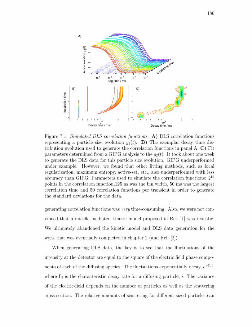
186
x106
10-6
10-5
10-4
10-3
10-2
decay time / ms
Autocorrelation g2(t)
Incubation tim
e
Lag time / ms
Incubation time
Decay time / ms
3 4 5 6 7 8 9
10-4
2 33 4 5 6 7 8 9
10-4
2 3
Decay time / ms
A)
B) C)
Figure 7.1: Simulated DLS correlation functions. A) DLS correlation functionsrepresenting a particle size evolution g2(t). B) The exemplar decay time dis-tribution evolution used to generate the correlation functions in panel A. C) Fitparameters determined from a GIPG analysis to the g2(t). It took about one weekto generate the DLS data for this particle size evolution. GIPG underperformedunder example. However, we found that other fitting methods, such as localregularization, maximum entropy, active-set, etc., also underperformed with lessaccuracy than GIPG. Parameters used to simulate the correlation functions: 219
points in the correlation function,125 ns was the bin width, 50 ms was the largestcorrelation time and 50 correlation functions per transient in order to generatethe standard deviations for the data.
generating correlation functions was very time-consuming. Also, we were not con-
vinced that a micelle mediated kinetic model proposed in Ref. [1] was realistic.
We ultimately abandoned the kinetic model and DLS data generation for the
work that was eventually completed in chapter 2 (and Ref. [2]).
When generating DLS data, the key is to see that the fluctuations of the
intensity at the detector are equal to the square of the electric field phase compo-
nents of each of the diffusing species. The fluctuations exponentially decay, e−Γit,
where Γi is the characteristic decay rate for a diffusing particle, i. The variance
of the electric-field depends on the number of particles as well as the scattering
cross-section. The relative amounts of scattering for different sized particles can
187
be estimated by a Gaussian random variable with a mean of zero and a standard
deviation equal to the square root of the characteristic scattering intensity for that
size (and shape) particle. We then impose the correlation that each species ex-
hibits onto the electric-field trajectory. Adding the resulting electric-fields yields
the net electric-field trajectory. The electric-field squared gives intensity trajec-
tory. To make intensity trajectory realistic, shot noise is added. Autocorrelating
the resulting trajectory yields the intensity correlation function often referred to
as g2(t). This data now has noise due to both the electric-field and intensity com-
ponents. Replicate transients can be generated in order to calculate the standard
deviation of the data.
Fig. 7.1 shows the evolution of generated correlation functions when the pep-
tide concentration is at the critical micelle concentration. The particle evolution
was generated by numerically solving the differential equations in Ref. [1]. The
particle size is related to a diffusion constant via the Stokes-Einstein equation.
The decay time evolution is then related to the diffusion through scattering vec-
tor, Di = Γi/q2 (see chapter 3). The intensity of each scattering particle was
estimated by:
Ii = CA3Na
(2πMwi (dn/dc)
Naλ2D
)2
Io (7.1)
where C is the concentration, A is the area of the detector, Mw is the average
molecular weight of particle, (dn/dc) is the index of refraction change, Na is
Avogadro’s Number, λ is the wavelength of the incident light, D is the distance
to the detector and Io is the incident light power. The total intensity of all the
particles for each transient was scaled to 300 kHz.
7.2.1 Generating DLS data, IGOR code
Function sim_ACF_photons(simpnts,tres,taumax, int)
variable simpnts,tres,taumax, int

188
Wave int_factor, rel_conc, tau
variable/g AvgRate
//simpnts = numpnts in the correlation function
//tres = bin width (xscale of correlation)
//taumax = the longest correlation for a particle size
//int = the laser intensity scale factor to keep the count
// rates reasonable.
//Tau is the correlation time for g1 not for g2. You can
//change this if you so desire.
//Intensity factor is the relative scattering intensity,
//not the correlation amplitude or the electric field
//amplitude.
//Rel_conc is the relative concentration.
//The first function includes just the correlated noise
//contributions. The second function also
//scales for the proper overall scattering intensity
//and generates the ACF with only correlated noise
//(sim) and the ACF with both types of noise (phot).
// closestgoodFFT is a list of good fft numbers
make /o/n=(closestgoodFFT(simpnts)) sim=0,temp=0,phot=0
make /o/n=(closestgoodFFT(taumax/tres)) dls_cor = 0
SetScale/P x 0,tres,"s", dls_cor, sim, temp, phot

189
sim=0
variable ind=0, sumwave = 0, holdsigma
do
if(int_factor[ind] > 0)
holdsigma=sqrt(int_factor[ind]*int*tau[ind]*2)
temp = gnoise(holdsigma) // calculates var. of intensity
dls_cor=exp(-x/tau[ind])// calculates decay function
sumwave = sum(dls_cor)
dls_cor /= sumwave //normalization
Correlate/c dls_cor, temp // correlated noise of e-field
sim+=temp //add them all together
endif
ind+=1
while (ind<numpnts(int_factor))
fastop sim=sim*sim // square to get intensity traj.
AvgRate += mean(sim)
AvgRate/=tres
phot=poissonNoise(sim) // Shot noise
variable mean_phot = mean(phot)
phot=(phot-mean_phot)/mean_phot
correlate phot phot // Autocorrelate for g2(t)
End
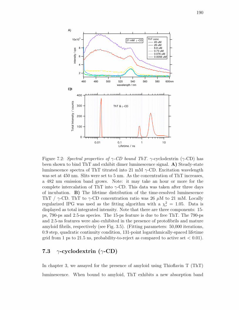
190
10x103
8
6
4
2intensity / cps
600nm580560540520500480460
wavelength / nm
ThT conc 45 uM 26 uM 8.8 uM 0.73 uM 0.076 uM 0.0056 uM
21 mM !!!-CD
!!!-CD
A)
B)
Figure 7.2: Spectral properties of γ-CD bound ThT. γ-cyclodextrin (γ-CD) hasbeen shown to bind ThT and exhibit dimer luminescence signal. A) Steady-stateluminescence spectra of ThT titrated into 21 mM γ-CD. Excitation wavelengthwas set at 450 nm. Slits were set to 5 nm. As the concentration of ThT increases,a 482 nm emission band grows. Note: it may take an hour or more for thecomplete intercalation of ThT into γ-CD. This data was taken after three daysof incubation. B) The lifetime distribution of the time-resolved luminescenceThT / γ-CD. ThT to γ-CD concentration ratio was 26 µM to 21 mM. Locallyregularized IPG was used as the fitting algorithm with a χ2
r = 1.05. Data isdisplayed as total integrated intensity. Note that there are three components: 15-ps, 790-ps and 2.5-ns species. The 15-ps feature is due to free ThT. The 790-psand 2.5-ns features were also exhibited in the presence of protofibrils and matureamyloid fibrils, respectively (see Fig. 3.5). (Fitting parameters: 50,000 iterations,0.9 step, quadratic continuity condition, 131-point logarithmically-spaced lifetimegrid from 1 ps to 21.5 ns, probability-to-reject as compared to active set < 0.01).
7.3 γ-cyclodextrin (γ-CD)
In chapter 3, we assayed for the presence of amyloid using Thioflavin T (ThT)
luminescence. When bound to amyloid, ThT exhibits a new absorption band
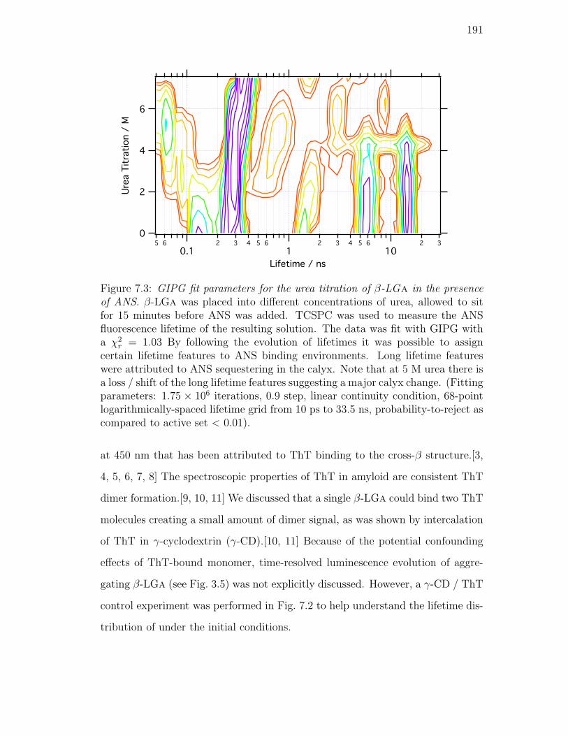
191
6
4
2
0
Ure
a T
itra
tion /
M
5 6
0.12 3 4 5 6
12 3 4 5 6
102 3
Lifetime / ns
Figure 7.3: GIPG fit parameters for the urea titration of β-LGa in the presenceof ANS. β-LGa was placed into different concentrations of urea, allowed to sitfor 15 minutes before ANS was added. TCSPC was used to measure the ANSfluorescence lifetime of the resulting solution. The data was fit with GIPG witha χ2
r = 1.03 By following the evolution of lifetimes it was possible to assigncertain lifetime features to ANS binding environments. Long lifetime featureswere attributed to ANS sequestering in the calyx. Note that at 5 M urea there isa loss / shift of the long lifetime features suggesting a major calyx change. (Fittingparameters: 1.75 × 10⁶ iterations, 0.9 step, linear continuity condition, 68-pointlogarithmically-spaced lifetime grid from 10 ps to 33.5 ns, probability-to-reject ascompared to active set < 0.01).
at 450 nm that has been attributed to ThT binding to the cross-β structure.[3,
4, 5, 6, 7, 8] The spectroscopic properties of ThT in amyloid are consistent ThT
dimer formation.[9, 10, 11] We discussed that a single β-LGa could bind two ThT
molecules creating a small amount of dimer signal, as was shown by intercalation
of ThT in γ-cyclodextrin (γ-CD).[10, 11] Because of the potential confounding
effects of ThT-bound monomer, time-resolved luminescence evolution of aggre-
gating β-LGa (see Fig. 3.5) was not explicitly discussed. However, a γ-CD / ThT
control experiment was performed in Fig. 7.2 to help understand the lifetime dis-
tribution of under the initial conditions.
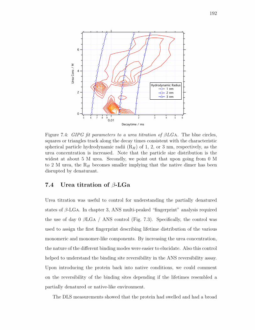
192
6
4
2
0
Ure
a C
onc /
M
5 6 7 8 9
0.012 3 4 5 6
Decaytime / ms
Hydrodynamic Radius 1 nm
2 nm
3 nm
Figure 7.4: GIPG fit parameters to a urea titration of βLGa. The blue circles,squares or triangles track along the decay times consistent with the characteristicspherical particle hydrodynamic radii (RH) of 1, 2, or 3 nm, respectively, as theurea concentration is increased. Note that the particle size distribution is thewidest at about 5 M urea. Secondly, we point out that upon going from 0 Mto 2 M urea, the RH becomes smaller implying that the native dimer has beendisrupted by denaturant.
7.4 Urea titration of β-LGa
Urea titration was useful to control for understanding the partially denatured
states of β-LGa. In chapter 3, ANS multi-peaked “fingerprint” analysis required
the use of day 0 βLGa / ANS control (Fig. 7.3). Specifically, the control was
used to assign the first fingerprint describing lifetime distribution of the various
monomeric and monomer-like components. By increasing the urea concentration,
the nature of the different binding modes were easier to elucidate. Also this control
helped to understand the binding site reversibility in the ANS reversibility assay.
Upon introducing the protein back into native conditions, we could comment
on the reversibility of the binding sites depending if the lifetimes resembled a
partially denatured or native-like environment.
The DLS measurements showed that the protein had swelled and had a broad

193
distribution of hydrodynamic radius. In a titration from 0 M to 7 M urea
(Fig. 7.4), the width of the DLS RH distribution was broadest at 5 M urea.
Since the width of the distribution was resolvable, this implied the exchange
time within that distribution was longer than the characteristic diffusion time of
∼20 µs for the monomer. Amyloid formation from βLGa has been observed to be
fastest at 5 M urea.[7] The day 0 DLS results showed that the conditions giving
the maximum rate of amyloidogenesis were coincident with those that created the
maximum variance in the hydrodynamic radius of βLGa.
194
References
[1] A. Lomakin, D. B. Teplow, D. A. Kirschner, G. B. Benedek, Kinetic theoryof fibrillogenesis of amyloid β-protein, Proc. Natl . Acad. Sci . USA 94 (1997)7942–7947.
[2] J. T. Giurleo, D. S. Talaga, Global fitting without a global model: Regular-ization based on the continuity of the evolution of parameter distributions,The Journal of Chemical Physics 128 (2008) 114114–(1–18).
[3] F. S. Waldrop, H. Puchtler, S. N. Meloan, Fluorescent thiazole stains foramyloid without differentiation, Journal of Histotechnology 7 (3) (1984) 123–126.
[4] A. Elhaddaoui, A. Delacourte, S. Turrell, Spectroscopic study of congo redand thioflavin binding to amyloid-like proteins, J. Mol. Struct. 294 (1993)115–118.
[5] I. LeVine, Harry, Thioflavine t forms uniquely fluorescent complexes withamyloid structures of synthetic alzheimer’s disease β-amyloid peptides andinsulin in solution, Amyloid Amyloidosis 1993, Proc. Int. Symp. Amyloidosis,7th (1994) 383–385.
[6] I. LeVine, Harry, Thioflavine t interaction with amyloid β-sheet structures,Amyloid 2 (1) (1995) 1–6.
[7] D. Hamada, C. M. Dobson, A kinetic study of β-lactoglobulin amyloid fibrilformation promoted by urea, Protein Sci. 11 (10) (2002) 2417–2426.
[8] T. Ban, D. Hamada, K. Hasegawa, H. Naiki, Y. Goto, Direct observation ofamyloid fibril growth monitored by thioflavin t fluorescence, J. Biol. Chem.278 (19) (2003) 16462–16465.
[9] R. Schirra, Dye aggregation in freezing aqueous solutions, Chem. Phys. Lett.119 (1985) 463–466.
[10] R. R. C. Retna Raj, γ-cyclodextrin induced intermolecular excimer formationof thioflavin t, Chem. Phys. Lett. 273 (1997) 285–290.
[11] M. Groenning, L. Olsen, M. van de Weert, J. M. Flink, S. Frokjaer, F. S.Jørgensen, Study on the binding of thioxavin t to β-sheet-rich and non-β–sheet cavities, Journal of Structural Biology 158 (2007) 358–369.
195
Chapter 8
Explanation of Global Regularization Code
8.1 Summary
In this chapter, the computational set up and implimentation of the globally
regularized interior point gradient method (GIPG) is described. First, the code
is introduced and the options are described. Next, there is an explanation of
the fast regularized GIPG using three dimensional matrix multiplications. This
procedure decreased overall computation by at least an order of magnitude, as
compared the method described in chapter 2. Flow charts are provided to help
navigate through the IGOR source code. The code itself is written in IGOR 6.03
format and found chapter 9.
8.2 Introduction
Globally regularized interior point gradient method (GIPG) [1] was developed
using IGOR Pro (WaveMetrics) platform. IGOR was chosen due to its built in
curve-fitting capabilities, ability to handle large data sets, implimenation of fast
matrix operations (LAPACK libraries), high speed data displaying and user pro-
gramming environment which allows for automation. Throughout this chapter,
we employ a few terms from the IGOR vernacular, including the terms “wave”
(short for waveform) to describe single column array of numbers contained in
the rows, matrix to describe waves with multiple columns, and 3D matrix as a
matrix with multiple layers. Lastly, the term x-scaling refers to abscissa values
196
corresponding to a wave if plotted on the ordinate.
GIPG only requires three inputs: the data, a design matrix, and number of
iterations. However, the typical GIPG user may prefer set up options to expedite
the implementation GIPG for a host fitting applications. IGOR’s pop up menu
capabilities serves as a useful tool for entering inputs such as:
• data
• options
• parameters.
To run the globally regularized IPG code, one must include the data which is to
be fit and a set of basis functions to fit them. The basis functions can be supplied
as either a set of “fingerprints” or as a grid of exponentials. For global fitting, the
data must be supplied as a matrix, with each column of the matrix representing a
single data transient. The order of the data waves within the data matrix should
correspond to a continuity condition that the GIPG algorithm implies. Secondary
data inputs include instrument response functions matrix and shift constants wave
(for convolution of data), standard deviations matrix and x-scaling wave of the
data. For secondary data matrices, their columns should match the corresponding
columns in the data matrix.
GIPG has already been utilized to globally fit time-correlated single-photon
counting [2], temperature-dependent Stokes-shift steady state fluorescence [3],
dynamic light scattering [2] data sets. Deconvolution of circular dichroism or
infrared absorption spectra also can be fit using regularized GIPG if altering an
experimental variable results in a continuity of the fit parameters. Several options
have been made available to facilitate the general applicability of fitting a variety
of spectroscopic data sets. The options include:
• setting the standard deviations equal to the square root of the data,
197
• invoking the Seigert relation for IPG fitting homodyne dynamic light scat-
ting data,
• convoluting of a fingerprint matrix by a grid of exponential functions,
• regularizing using linear or quadratic continuity condition or local maximum
entropy method,
• selecting a range of grid points to regularize,
• fitting locally or globally,
• pre-normalizing data and standard deviations,
• calculating effective free parameters,
• estimating time to complete fit,
• and/or saving the fit results.
These options should allow for fitting various data set types using different
methods. In chapter 3 of this thesis, there are examples of regularized GIPG
fitting with some of these options implemented. For example, Seigert relation was
used to globally fit the dynamic light scattering data of an aggregating protein
along a timecourse. Time-correlated single-photon counting was used to measure
evolution fluorescence lifetime distributions of an extrinsically labeled protein
over time. The data was first fit using a grid of convoluted exponential decays
to obtain a set of lifetime distribution fingerprints. The data was then fit using
instrument response convoluted fingerprints to generate a global model of reduced
parameters. Maximum entropy method was added by popular demand. It utilized
IGOR’s built in curvefit capabilities. Unfortunately, it is unstable for large data
sets (several hundred parameters) and is to be used at your own risk.
The user must set a few parameters before the fit can be started. They include:
198
• strength of regularizer
• number of iterations
• size of each IPG step
• and number of display updates.
Once the fitting has started, there are several displays for user evalution, such as,
• a fit window containing the x-scaled data, the fit, calculated reduced chi-
squared (χ2r), change in χ2
r, and a counter for the remaining updates
• fit parameters vs basis function coordinate
• and plot of χ2r and probability-to-reject vs update number
GIPG (and for that matter, IPG) is an iterative fitting method without an explic-
itly defined convergence criteria. Instead, the user inputs the number of iterations
to perform. After completion, the user decides if the fit has converged. For con-
venience, the algorithm displays useful parameters mentioned in the list above,
and greater detail in chapter 2 of this thesis. Many users may decide that if χ2r is
close to 1.0, and/or the change of χ2r is very small, and/or probability-to- reject
< 0.5, the algorithm has converged.
8.2.1 Fast GIPG
Recall the minimization principle in Methods section of chapter 2,
(ATl Al + γH)xl −AT
l bl = 0, (8.1)
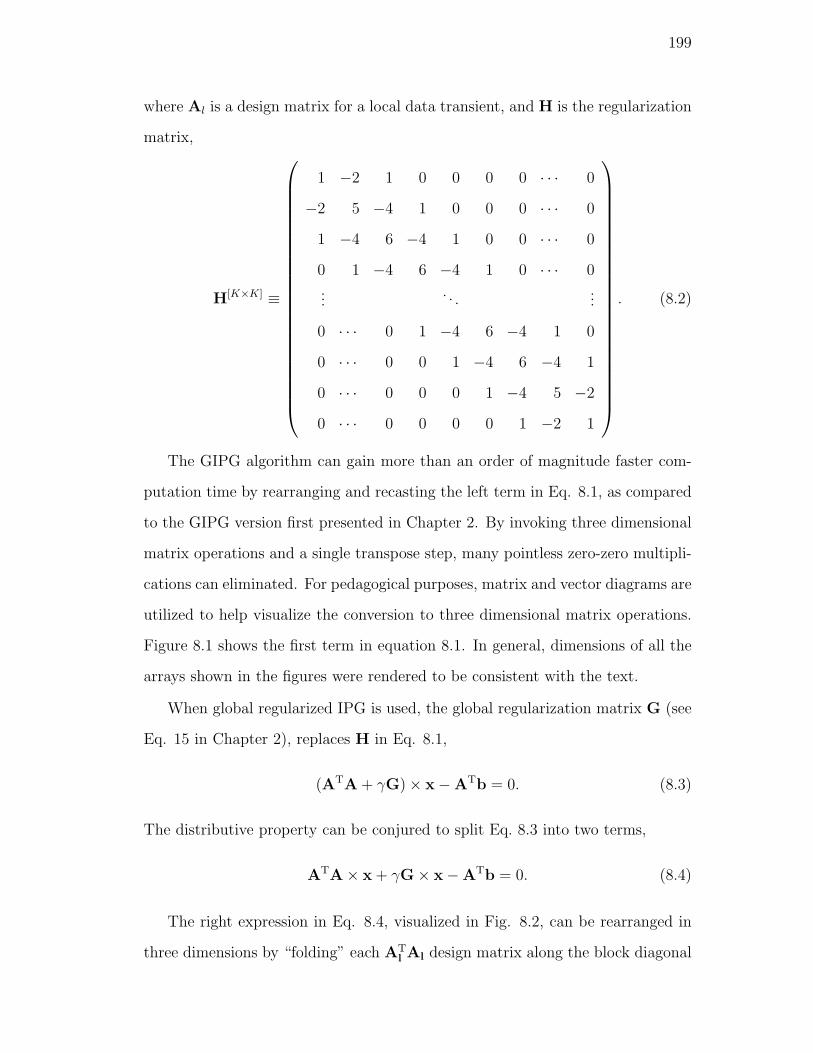
199
where Al is a design matrix for a local data transient, and H is the regularization
matrix,
H[K×K] ≡
1 −2 1 0 0 0 0 · · · 0
−2 5 −4 1 0 0 0 · · · 0
1 −4 6 −4 1 0 0 · · · 0
0 1 −4 6 −4 1 0 · · · 0
.... . .
...
0 · · · 0 1 −4 6 −4 1 0
0 · · · 0 0 1 −4 6 −4 1
0 · · · 0 0 0 1 −4 5 −2
0 · · · 0 0 0 0 1 −2 1
. (8.2)
The GIPG algorithm can gain more than an order of magnitude faster com-
putation time by rearranging and recasting the left term in Eq. 8.1, as compared
to the GIPG version first presented in Chapter 2. By invoking three dimensional
matrix operations and a single transpose step, many pointless zero-zero multipli-
cations can eliminated. For pedagogical purposes, matrix and vector diagrams are
utilized to help visualize the conversion to three dimensional matrix operations.
Figure 8.1 shows the first term in equation 8.1. In general, dimensions of all the
arrays shown in the figures were rendered to be consistent with the text.
When global regularized IPG is used, the global regularization matrix G (see
Eq. 15 in Chapter 2), replaces H in Eq. 8.1,
(ATA + γG)× x−ATb = 0. (8.3)
The distributive property can be conjured to split Eq. 8.3 into two terms,
ATA× x + γG× x−ATb = 0. (8.4)
The right expression in Eq. 8.4, visualized in Fig. 8.2, can be rearranged in
three dimensions by “folding” each ATl Al design matrix along the block diagonal
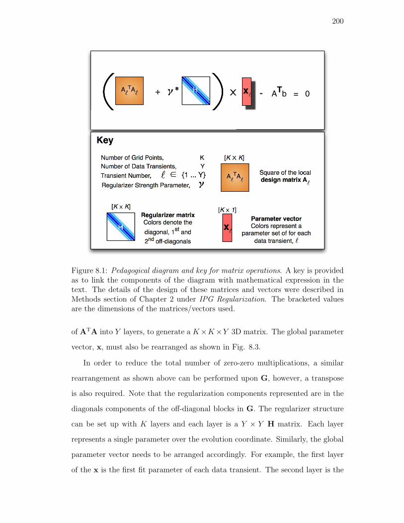
200
Al
TAl
Hγ*+
H
Regularizer matrixColors denote the
diagonal, 1st and
2nd off-diagonals
[K ⨉ K]
Parameter vector Colors represent a
parameter set of for each
data transient, l
[K ⨉ 1]
Number of Grid Points, K
Number of Data Transients, Y
l ∈ 1 ... YTransient Number,
Regularizer Strength Parameter, γ Al
TAl
[K ⨉ K]
Square of the localdesign matrix A
l
Key
xl
xl - ATb = 0
Figure 8.1: Pedagogical diagram and key for matrix operations. A key is providedas to link the components of the diagram with mathematical expression in thetext. The details of the design of these matrices and vectors were described inMethods section of Chapter 2 under IPG Regularization. The bracketed valuesare the dimensions of the matrices/vectors used.
of ATA into Y layers, to generate a K×K×Y 3D matrix. The global parameter
vector, x, must also be rearranged as shown in Fig. 8.3.
In order to reduce the total number of zero-zero multiplications, a similar
rearrangement as shown above can be performed upon G, however, a transpose
is also required. Note that the regularization components represented are in the
diagonals components of the off-diagonal blocks in G. The regularizer structure
can be set up with K layers and each layer is a Y × Y H matrix. Each layer
represents a single parameter over the evolution coordinate. Similarly, the global
parameter vector needs to be arranged accordingly. For example, the first layer
of the x is the first fit parameter of each data transient. The second layer is the
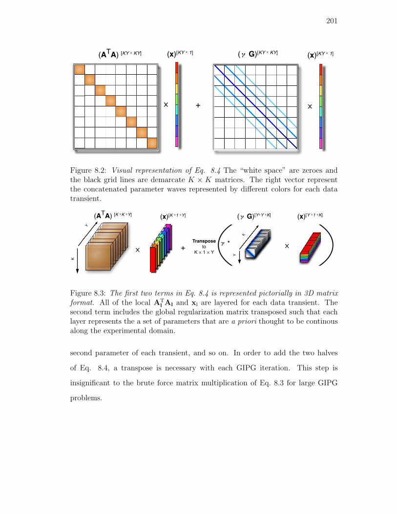
201
+
(x)[KY ⨉ 1] (ATA) [KY ⨉ KY] (γ G)[KY ⨉ KY] (x)[KY ⨉ 1]
Figure 8.2: Visual representation of Eq. 8.4 The “white space” are zeroes andthe black grid lines are demarcate K × K matrices. The right vector representthe concatenated parameter waves represented by different colors for each datatransient.
Y
K
+γ *
K
Transpose
to
K ⨉ 1 ⨉ Y
Y
(γ G)[Y⨉Y ⨉K] (x)[Y ⨉1 ⨉K] (ATA) [K ⨉K ⨉Y] (x)[K ⨉1 ⨉Y]
Figure 8.3: The first two terms in Eq. 8.4 is represented pictorially in 3D matrixformat. All of the local AT
l Al and xl are layered for each data transient. Thesecond term includes the global regularization matrix transposed such that eachlayer represents the a set of parameters that are a priori thought to be continousalong the experimental domain.
second parameter of each transient, and so on. In order to add the two halves
of Eq. 8.4, a transpose is necessary with each GIPG iteration. This step is
insignificant to the brute force matrix multiplication of Eq. 8.3 for large GIPG
problems.
202
8.3 Flow charts
Flow charts were developed to help user understand the actions of the source
code. Fig. 8.4 shows the overall structure of the GIPG, including a key which
is applicable to all of the subsequenct schemes. Colored boxes point to high-
light very important steps. Fig. 8.5 describes the setup of the relevant design
and regularization matrix depending on type of basis functions chosen. Also,
this is where the appropriate data, standard deviations, and x-scaling waves are
prepared. Setup Reg Part1 in Fig. 8.6 is potentially slowest step of the GIPG
algorithm. Normalization and calculation of the effective free parameters are also
performed.
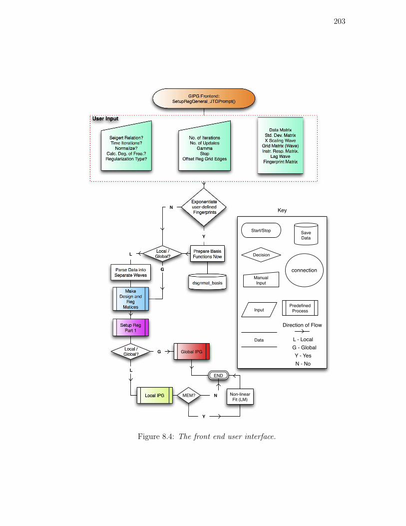
203
User Input
GIPG Frontend:
SetupRegGeneral_JTGPrompt()
Data Matrix
Std. Dev. Matrix
X Scaling Wave
Grid Matrix (Wave)
Instr. Resp. Matrix.
Lag Wave
Fingerprint Matrix
Seigert Relation?
Time Iterations?
Normalize?
Calc. Deg. of Free.?
Regularization Type?
Exponentiate
user-defined
Fingerprints
Prepare Basis
Functions Now
Local /
Global?L
Y
N
Parse Data into
Separate Waves
Make
Design and
Reg
Matices
G
No. of Iterations
No. of Updates
Gamma
Step
Offset Reg Grid Edges
dsgnmat_basis
Setup Reg
Part 1
Local /
Global?
L
Local IPG
Global IPGG
END
MEM?
Y
Non-linear
Fit (LM)
Manual
Input
Save
Data
InputPredefined
Process
Decision
connection
Start/Stop
Direction of Flow
G - Global
L - Local
N - No
Y - Yes
Data
Key
N
Figure 8.4: The front end user interface.
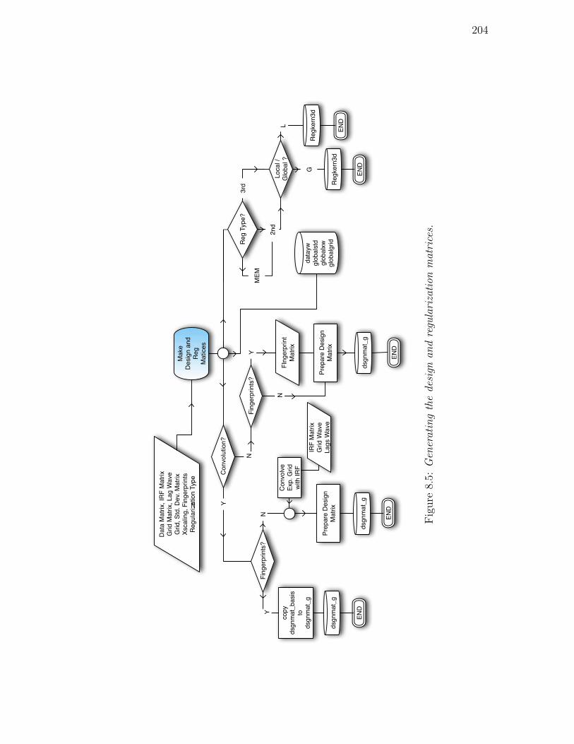
204
Make
Design and
Reg
Matices
Reg Type?
3rd
2nd
MEM
Local /
Global ?
Regkern3d
Convolution?
Y
N
Fingerprints?
NY
dsgnmat_g
dsgnmat_g
IRF Matrix
Grid Wave
Lags Wave
Prepare Design
Matrix
copy
dsgnmat_basis
to
dsgnmat_g
Convolve
Exp. Grid
with IRF
Fingerprints?
Y
N
Prepare Design
Matrix
FIngerprint
Matrix
dsgnmat_g
END
END
END
END
G
L
Regkern3d
END
Data Matrix, IRF Matrix
Grid Matrix, Lag Wave
Grid, Std. Dev. Matrix
Xscaling, Fingerprints
Regularization Type
datayw
globalstd
globalxw
globalgrid
Fig
ure
8.5:
Gen
erat
ing
the
desi
gnan
dre
gula
riza
tion
mat
rice
s.
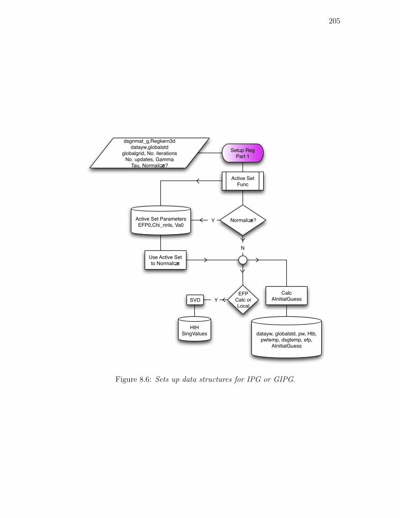
205
Setup Reg
Part 1
Active Set
Func
Active Set Parameters
EFP0,Chi_nnls, Va0
dsgnmat_g,Regkern3d
datayw,globalstd
globalgrid, No. iterations
No. updates, Gamma
Tau, Normalize?
EFP
Calc or
LocalYSVD
HtH
SingValues datayw, globalstd, pw, Htb,
pwtemp, dsgtemp, efp,
AInitialGuess
Calc
AInitialGuess
Normalize?Y
N
Use Active Set
to Normalize
Figure 8.6: Sets up data structures for IPG or GIPG.
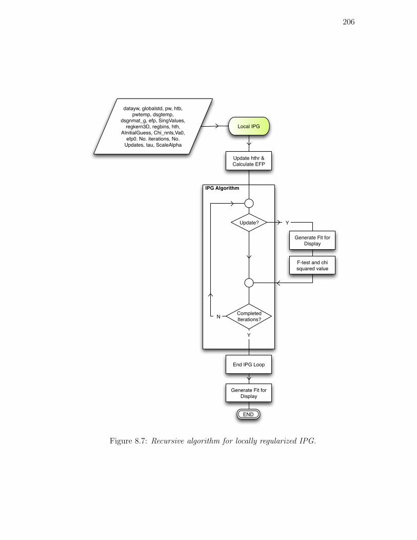
206
Local IPG
datayw, globalstd, pw, htb,
pwtemp, dsgtemp,
dsgnmat_g, efp, SingValues,
regkern3D, regbins, hth,
AInitialGuess, Chi_nnls,Va0,
efp0. No. iterations, No.
Updates, tau, ScaleAlpha
Update hthr &
Calculate EFP
IPG Algorithm
End IPG Loop
Update?
Generate Fit for
Display
F-test and chi
squared value
Y
Completed
Iterations?
Y
N
Generate Fit for
Display
END
Figure 8.7: Recursive algorithm for locally regularized IPG.
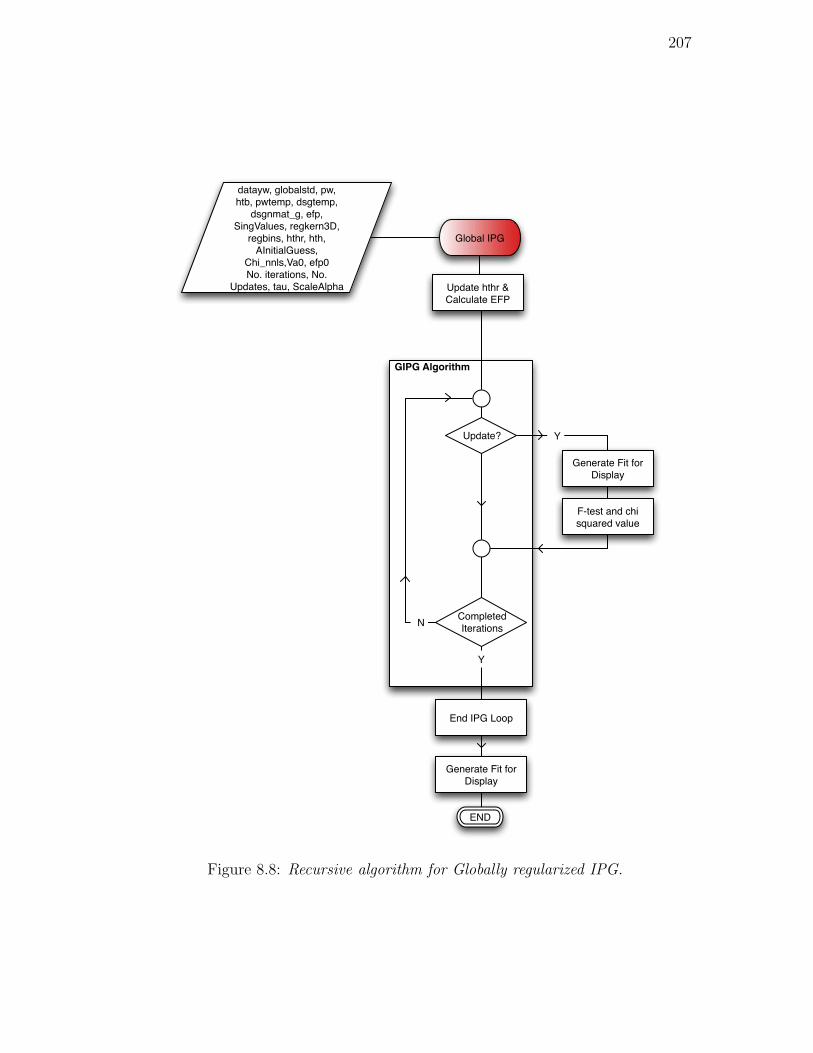
207
Global IPG
datayw, globalstd, pw,
htb, pwtemp, dsgtemp,
dsgnmat_g, efp,
SingValues, regkern3D,
regbins, hthr, hth,
AInitialGuess,
Chi_nnls,Va0, efp0
No. iterations, No.
Updates, tau, ScaleAlpha
GIPG Algorithm
End IPG Loop
Update?
Generate Fit for
Display
F-test and chi
squared value
Y
Completed
Iterations
Y
N
Generate Fit for
Display
END
Update hthr &
Calculate EFP
Figure 8.8: Recursive algorithm for Globally regularized IPG.
208
References
[1] Jason T. Giurleo and David S. Talaga. Global fitting without a global model:Regularization based on the continuity of the evolution of parameter distri-butions. The Journal of Chemical Physics, 128:114114–(1–18), 2008.
[2] Jason T. Giurleo, Xianglan He, and David S. Talaga. β-lactoglobulin assem-bles into amyloid through sequential aggregated intermediates. J. Mol. Bio.,381:1332–1348, 2008.
[3] Jeremy Pronchik, J. T. Giurleo, and David S. Talaga. Analysis of dynamicstokes shift with multiple fluorescence environments: Coumarin 153 in bovineβ-lactoglobulin a. J. Phys. Chem. B, 112:11422–11434, 2008.
209
Chapter 9
Globally regularized interior point gradient
method, Igor code
//Global Regularization
//Developed by Jason T. Giurleo on Feb 17, 2007
//Version 1.0 by May 2008
// The commented number - letter refer to the top function@
//and its subfunctions
#pragma rtGlobals=1// Use modern global access method.
Menu "Macros"
"Graph or Table to Matrix", Trace2TablePrompt()
"Truncate Your Matrices",
TruncateDataMatrix_Prompt()
"Find The Best IRF ", FindTheBestIRF_Prompt()
"Make A Grid", MakeAGrid_Prompt()
"Setup GIPG Fit ", SetupRegGeneral_JTGPrompt()
"Continue GIPG Fit", GIPGContinued()
End
// Table of Contents
//1 - A Trace2TablePrompt//4 - A MakeAGrid_Prompt
//1 - B Trace2Table//4 - B MakeLogGridname
//
210
//2 - A TruncateDataMatrix_Prompt//5 - A SetupReg@
//General_JTGPrompt
//2 - B SetCursors1//5 -B MakeDesignandRegMatices
//2 - C SetCursors2//5 - C MakeRegMatrix
//2 - D UserCursorAdjust//5 - D SetupGIPG_part1
//2 - E UserCursorAdjust_ContButtonProc//5 - E LoopActiveSet
//5 - F ActiveSetFunc
////5 - G Global_IPG
//3 - A FindTheBestIRF_Prompt//5 - H MultexpMEM
//3 - B FindTheBestIRF //5 - I CalcFtest
//3 - C Create_LimitWv//5 - J fdist
//3 - D FitConvIRFMultExp//5 - K Local_IPG
//6 - A GIPGContinued
//
//**** EXTRAS ****
//DLS_Loader
//OrganizeDLS
//calctau
//calcRad
//AsciiWithSetup (for Becker-Hickl TCSPC asc files with@
//setup)
//***** 1 - A ***** \\
Function Trace2TablePrompt()
String WindowName_STR = StrVarOrDefault("Root@
:JTG_IPGfolder:gWindowName_STR", "WindowName")
String MatrixName_STR = StrVarOrDefault("Root:J@
211
TG_IPGfolder:gMatrixName_STR", "MatrixName")
Prompt WindowName_STR,"Name of the window @
containing data traces or columns"
Prompt MatrixName_STR,"Name matrix to put data@
in"
DoPrompt "Convert Graph or Table to Matrix", @
WindowName_STR, MatrixName_STR
Trace2Table(WindowName_STR, MatrixName_STR)
If (DataFolderExists("root:JTG_IPGfolder") == 0)
NewDataFolder root:JTG_IPGfolder
EndIf
String savedDataFolder = GetDataFolder (1)
// save
SetDataFolder Root:JTG_IPGfolder:
String/g gWindowName_STR = WindowName_S@
TR, gMatrixName_STR = MatrixName_STR
SetDataFolder savedDataFolder// and restore
End
//***** 1 - B ***** \\
Function Trace2Table(WindowName, MatrixName)
//This function will place all the waves in the specIfied @
//graph or table window into a matrix.

212
String WindowName, MatrixName windowname = "WIN:"+
windowname
String Wvlist = WaveList("*", ";",WindowName)
Variable ii = 0, numwvs = ItemsInList(WvList)
String wvnm = StringFromList(ii, WvList) // gets waves from
//list
Duplicate/o $wvnm wv
Variable dx = deltax(wv)// x scaling If it exists.
Variable pts = numpnts(wv)
Make/o/n=(pts , numwvs) GraphMat
do
wvnm = StringFromList(ii, WvList)
Duplicate/o $wvnm wv
GraphMat[][ii] = wv[p]
ii+=1
while(ii < numwvs)
SetScale/P x 0, dx,"", Graphmat// scales matrix
Duplicate/o Graphmat $matrixname
Killwaves/z Wv, GraphMat
End
//***** Conclusion of 1 ***** \\
//***** 2 - A ***** \\
Function TruncateDataMatrix_Prompt()
Make/o/n=0 ’Data is X scaled’
213
String datamat_STR = StrVarOrDefault("Root:JTG_IPG@
folder:gDatatrunc_str", "MatrixName")
String secondwave_STR = StrVarOrDefault("Root:JTG_@
IPGfolder:gIRFtrunc_str", "MatrixName")
String XWAVE_STR = strVarOrDefault("Root:JTG_IPG@
folder:gXWAVE_str", "XwaveName")
Prompt datamat_STR, "Data Matrix", popup, Wavelist("*",@
";", "")
Prompt secondwave_STR,"IRF Matrix or STD Matrix", @
popup, Wavelist("*", ";", "")
Prompt XWAVE_STR,"Choose an X-scaling Wave (If @
necessary)", popup, Wavelist("*", ";", "")
DoPrompt "Truncation", datamat_STR, secondwave_ST@
R, XWAVE_STR
If(V_flag ==1)
Abort "User Cancelled Truncation"
EndIf
If (DataFolderExists("root:JTG_IPGfolder") == 0)
NewDataFolder root:JTG_IPGfolder
EndIf
String savedDataFolder = GetDataFolder(1)// save
SetDataFolder Root:JTG_IPGfolder:
String/g gDatatrunc_str = datamat_STR, gIRFtrunc_str = @
secondwave_STR, gXWAVE_str = XWAVE_STR
SetDataFolder savedDataFolder// and restore
214
If(cmpstr(XWAVE_STR, NameOfWave(’Data is X scaled’)) @
== 0)
Make/o/n=1e8 dumx = 0
XWAVE_STR = "dumx"
EndIf
SetCursors1(datamat_STR, secondwave_STR, XWAVE_@
STR)
killwaves/z dumx, dumx_trunc
End
//***** 2 - B ***** \\
Function SetCursors1(wvnm, irfwvnm, xw_str)
String wvnm, irfwvnm, xw_str
DoWindow/k Truncate_Window
Display $wvnm
ShowInfo
ModIfyGraph log(left)=1
DoWindow/c Truncate_Window
If (UserCursorAdjust("Truncate_Window") != 0)
return -1;
EndIf
SetCursors2(wvnm, irfwvnm, xw_str)
End
215
//***** 2 - C ***** \\
Function SetCursors2(wvnm, irfwvnm, xw_str)
String wvnm, irfwvnm, xw_str//cursors on the data wave@
//as you like.
String wave_trunc = wvnm + "_trunc"//set your cursons on @
//a data wave you want to
String irfwvnm_trunc= irfwvnm + "_trunc"
String xw_str_trunc = xw_str + "_trunc"
Variable start , finish, sr = screenresolution
If (strlen(csrinfo(A))==0)
start = 0
Print "Warning: Are you sure you Donot want to truncate @
your waves?!"
Else
start = pcsr(A)
EndIf
If (strlen(csrinfo(B))==0)
Finish = Dimsize($wvnm, 0)
Print "Warning: Are you sure you Do not want to truncate @
your waves?!"
Else
finish = pcsr(B)
EndIf
216
Finish = selectnumber(mod(finish-start, 2 )== 0, finish, @
Finish+1)
Duplicate/o $wvnm $wave_trunc
Duplicate/o $irfwvnm $irfwvnm_trunc
Duplicate/o $xw_str $xw_str_trunc
Redimension/n=(Finish,-1) $wave_trunc, $irfwvnm_trunc,@
$xw_str_trunc
Deletepoints 0, Start, $wave_trunc, $irfwvnm_trunc, $xw_@
str_trunc
If (DataFolderExists("root:JTG_IPGfolder") == 0)
NewDataFolder root:JTG_IPGfolder
EndIf
String savedDataFolder = GetDataFolder(1)// save
SetDataFolder Root:JTG_IPGfolder:
Variable/g gCursorFinish = Finish, gCursorStart = Start
SetDataFolder savedDataFolder
Dowindow/k Truncate_Window
End
//***** 2 - D ***** \\
Function UserCursorAdjust(grfName)

217
String grfName
DoWindow/F $grfName// Bring graph to front
If (V_Flag == 0)// VerIfy that graph exists
Abort "UserCursorAdjust: No such graph."
return -1
EndIf
NewPanel/K=2 /W=(139,341,382,432) as "Pause for @
Cursor"
DoWindow/C tmp_PauseforCursor// Set to an unlikely name
AutoPositionWindow/E/M=1/R=$grfName// Put panel near@
the graph
DrawText 21,20,"Adjust the cursors and then"
DrawText 21,40,"press Continue."
Button button0,pos=80,58,size=92,20,title="Continue"
Button button0,proc=UserCursorAdjust_ContButtonProc
PauseForUser tmp_PauseforCursor,$grfName
return 0
End
//***** 2 - E ***** \\
Function UserCursorAdjust_ContButtonProc(ctrlName) :@
ButtonControl
String ctrlName
DoWindow/K tmp_PauseforCursor// Kill self
218
End
/// ******* Conclusion of 2 *******///
//***** 3 - A ***** \\
Function FindTheBestIRF_Prompt()
// Prompt for finding the best IRF for a fit. See the@
//function FindTheBestIRF for explanation.
//The prompts just sets up the main function. The other @
//useful feature
//is If a initial guess parameter wave was not chosen, one@
//can be chosen for you.
// Need data, irfs and initial guesses (If available).
String datamat_STR = StrVarOrDefault("gdata_STR", @
"MatrixName")
String irfmat_STR = StrVarOrDefault("girf_STR",@
"MatrixName")
String InitialGuess = StrVarOrDefault("gInitialGuess", "Do @
a 2 Exp Fit, Makes a wave called W_coef")
Prompt datamat_STR, "Data Matrix", popup, Wavelist("*", "@
;" "")
Prompt irfmat_STR,"IRF Matrix", popup, Wavelist("*", ";", "")
Prompt InitialGuess, "Initial Parameter Wave", popup,"Do @
a 2 Exp Fit, makes a wave called W_coef;" + Wavelist("*", @
";", "")

219
DoPrompt "Find The BestIRF", datamat_STR, irfmat_STR,@
InitialGuess
If(V_flag ==1)
Abort "User Cancelled Quick Fits"
EndIf
String/g gdata_STR = datamat_STR, gIrf_Str = irfmat_@
STR, gInitialGuess = InitialGuess
Duplicate/o $datamat_STR Datamat_
Duplicate/o $irfmat_STR IRFmat_
// Sets up some dummy waves for fit.
Make/o/n=(dimsize(datamat_, 0)) SingleDataWave, Std@
SingleDataWave
SingleDataWave = Datamat_[p][0]
StdSingleDataWave = sqrt(Datamat_[p][0]+1)
SetScale/P x 0,deltax(Datamat_),"", SingleDataWave, Std@
SingleDataWave
WaveStats/q SingleDataWave
//If you want IGOR to Make initial guesses.
If( CmpStr(InitialGuess, "Do a 2 Exp Fit, Makes a wave @
called W_coef") == 0)
killwaves/z W_coef
CurveFit/n/q dblexp_XOffSet SingleDataWave[X2Pnt@
(SingleDataWave,V_maxLoc) + 50,Numpnts(SingleData@
Wave)-1] /W=StdSingleDataWave /I=1

220
Wave W_coef
Insertpoints 0, 1, W_coef
W_coef[0] = .01
Duplicate/o W_coef Epwv
FindTheBestIRF(Datamat_, W_coef, IRFmat_)
//otherwise
Else
Duplicate/o $InitialGuess DumCoefs
Duplicate/o DumCoefs Epwv
FindTheBestIRF(Datamat_, DumCoefs, IRFmat_)
Duplicate/o DumCoefs $InitialGuess
EndIf
Dowindow/K DiscreteFits
killwaves/z DumCoefs, Datamat_, IRFmat_, StdSingle@
DataWave, SingleDataWAve, W_sigma, W_fitConstants
killwaves/z Epwv, Fit_testwv, Stdtestwv, Holdwc, res_@
testwv, testwv, , res_Testwv, testwv, fit_testwv, lags
killwaves/z root:DiscreteParms, dum, epslnwv, fit_testwv,@
IM, instrument_response_, Lagmat, resmat, limitwv
End
//***** 3 - B ***** \\\
Function FindTheBestIRF(mat,wc, Allirfs)
// Many instrument response functions may be taken@
//throughout an experiment. To choose the best IRF for@
//any particular data trace, use this function. Every data@
//trace is fit via multiple exponential convolution fitting to@
//every available IRF. The chi squared values are saved. @
221
//The fits with the best IRFs’ will have the lowest chi @
//squared and are choosen and placed in a matrix called@
//’FinalIRFMatrix’. For added convenience,the lag@
//parameters corresponding,to the best IRFs are also @
//stored in a wave called ’finallags’.
// Mat == Data matrix
// wc == initial guesses for multiple exponential convolu@
//tion fitting
// allirfs == all the irfs that you have
wave mat, wc, allirfs
// Make data waves matrices If not already
If(dimsize(mat, 1)==0)
redimension/n=(-1, 1) mat
EndIf
If(dimsize(Allirfs, 1)==0)
redimension/n=(-1, 1) Allirfs
EndIf
//Set up some Variables.
Variable/g V_fitoptions = 4, V_FitMaxIters = 100, V_fitNum@
Iters, V_fiterror = 0 // curvefit Variables, see IGOR docume@
//ntation
Variable ii = 0, jj = 0
222
//Set up dummy waves for fitting
Make/o/n=(dimsize(mat, 1)) lags= 0, res = 0
Make/o/n=(dimsize(mat, 0)) testwv, stdtestwv, instrument_@
response_, fit_testwv = 0
SetScale/p x 0,deltax(mat),"", testwv, stdtestwv, instrument@
_response_, fit_testwv
Make/o/n=(numpnts(wc), dimsize(mat,1)) DiscreteParms
Duplicate/o wc holdwc
Make/o/n=(numpnts(wc)) epwv = 1e-6
// Make a fit window
dowindow/k discretefits
display testwv, fit_testwv
ModIfyGraph log(left)=1
ModIfyGraph rgb(fit_testwv)=(1,3,39321)
Dowindow/c Discretefits
Duplicate/o mat FinalIRFMatrix
Make/o/n=(numpnts(res), dimsize(Allirfs, 1)) resmat = 0
Make/o/n=(numpnts(res), dimsize(Allirfs, 1)) lagmat = 0
// Create a constraint wave, but remove the positivity const@
//raint on the first parameter (lag).
create_limitwv(wc)
deletepoints 0, 1, limitwv
do
223
instrument_response_ = Allirfs[p][jj]
do
Duplicate/o wc holdwc
testwv= mat[p][ii]
stdtestwv=sqrt( mat[p][ii] +1)// std. dev. always the square@
//root of the data.
FuncFit/q/ODR=1/L= (numpnts(testwv)) FitConvIRFMultEx@
p wc testwv /W=stdtestwv /I=1 /D /R/c=limitwv/E = EPWV
res[ii] = v_chisq
lags[ii] = wc[0]
DiscreteParms[][ii] = wc[p]
//If there is an error Dothe fit again with user input.
If(V_fiterror!=0)
dowindow/k parms
edit/K=1 wc, holdwc
dowindow/c parms
pauseforuser parms
Variable changed = wc -holdwc
If(changed == 0)
wc += (gnoise(WC/100))
EndIf
V_fiterror = 0
Else

224
ii +=1
EndIf
V_fiterror = 0
while(ii<dimsize(mat, 1))
// Record chi squared and lags in a matrix
resmat[][jj] = res[p]
lagmat[][jj] = lags[p]
ii = 0
jj+=1
while(jj<dimsize(allirfs, 1))
jj = 0
Variable v_minloc
Make/o/n=(dimsize(allirfs, 1)) dum = 0
Make/o/n=(dimsize(FinalIRFMatrix, 1)) finallags = 0
// Choose the lowest chi squared and its cooresponding @
//lag parameter and IRF.
do
dum[]= resmat[jj][p]
If(numpnts(dum)==1)
FinalIRFMatrix[][jj] = Allirfs[p][0]
finallags[jj] = lagmat[jj][0]
Else

225
wavestats/q dum
FinalIRFMatrix[][jj] = Allirfs[p][v_minloc]
finallags[jj] = lagmat[jj][v_minloc]
EndIf
jj +=1
while(jj<dimsize(FinalIRFMatrix, 1))
If(dimsize(mat, 1)==1)
redimension/n=(-1,0) mat
EndIf
If(dimsize(allirfs, 1)==1)
redimension/n=(-1,0) allirfs
EndIf
End
//***** 3 - C ***** \\
function create_LimitWv(grd)
//This function Makes a text wave in the form that curvefit@
//expects a constaint text wave.
//Also an epsilon wave is generated. The length of each
//wave is the same as the number of paramters inputted.
wave grd
Variable TotalGrid = numpnts(grd) , ii = 0
Make/o/n=(TotalGrid)/T LimitWv
String ks
226
do
ks = "K" + num2str(ii) + ">1e-6"
LimitWv[ii] = ks
ii +=1
while(ii<TotalGrid)
Make/d/o/n=(totalGrid) epslnwv = 1e-6
End
//***** 3 - D ***** \\
Function FitConvIRFMultExp(pw, yw, xw) : FitFunc
// Multiexponential convolution fitting of TCSPC data. This@
//function also allows for a lag parameter, which shIfts the @
//IRF by a fraction
// of a bin. This allows for very very small shIfts in the @
//IRF, without scarIficing chi squared.
// pw[0] = time lag
// pw[1] = baseline
// pw[2*m] = amp m
// pw[2*m+1] = exp rate m
Wave/Z pw, yw, xw
Variable dx=deltax(instrument_response_)
Variable npnts = numpnts(yw)
Duplicate/O instrument_response_, IM
Wave instrument_response_
227
Variable lag = pw[0]
IM = instrument_response_(p*dx+lag)
Variable IMsum = sum(IM, -inf, inf)
IM /= IMsum// normalize instrument response to 1.0
fastop yw = 0 // initialize model values to zero so we can
accumulate exponential terms
Variable numCoefs = numpnts(pw)// calculate number of@
//exponential terms desired
Variable ii=2
do
yw +=pw[ii]*exp(-pw[ii+1]*(p*dx))//DeltaX value is multipli@
//ed by each point in Xwave to get the proper
ii+=2//scaling and lag
While (ii<numCoefs)
If (mod(numcoefs,2)!=0)
yw[0]+=pw[numpnts(pw)-1]
endif
Convolve IM,yw// this operation lengthens yw to contain M@
//+N points, where M is length of instrument response, @
//and N is length of yw
yw+=pw[1]//baseline
redimension/N=(npnts)yw// this removes the extra points
End
/// ******* Conclusion of 3 *******///
//***** 4 - A ***** \\\
228
Function MakeAGrid_Prompt()
String traceName = StrVarOrDefault("Root:JTG_IPGfolder@
:gGrid", "ChooseAGridName")
String LogLin = StrVarOrDefault("Root:JTG_IPGfolder:gL@
oL", "Lin")
Variable Start = NumVarOrDefault("Root:JTG_IPGfolder:g@
Start", .1)
Variable Finish = NumVarOrDefault("Root:JTG_IPGfolder@
:gFinish",10)
Variable PntsPerDec= NumVarOrDefault("Root:JTG_IPG@
folder:gPntsPerDec",10)
Prompt LogLin, "Log or Linear", popup "Log;Linear;"
Prompt TraceName,"Name Your Grid"
Prompt Start, "First Point"
Prompt Finish, "Last Point"
Prompt PntsPerDec, "Points Per Decade (LOG) or@
Increments (LIN)"
DoPrompt "Make A Grid", Start, Finish, PntsPerDec, Trace@
Name, LogLin
If ( V_flag == 1)
abort "User Cancelled MakeAGrid"
EndIf
If (DataFolderExists("root:JTG_IPGfolder") == 0)
NewDataFolder root:JTG_IPGfolder
EndIf
229
String savedDataFolder = GetDataFolder(1)// save
SetDataFolder Root:JTG_IPGfolder:
Variable/G gStart = Start, gFinish = Finish, gPntsPerDec =@
PntsPerDec // Save for next time
String/g gGrid = tracename, gLoL = LogLin
SetDataFolder savedDataFolder // and restore
If(CmpStr(traceName, "ChooseAGridName")==0)
TraceName = "Grid"
Print "Because you didn’t pick name for the grid, I did... @
your grid is now called ... GRID"
EndIf
If( CmpStr(LogLin, "Log") == 0)
MakeLogGridname(Start, Finish, PntsPerDec, TraceName)
Print "Number of Points", numpnts($TraceName)
Else
Variable dum1 = Finish - Start, dum2 = floor(dum1/PntsPe@
rDec)
Make/o/n=(dum2) DumGrid = Start + PntsPerDec*p
Duplicate/o DumGrid $TraceName
Print "Number of Points", numpnts(DumGrid)
Killwaves/z DumGrid
EndIf
End
230
//***** 4 - B ***** \\\
Function MakeLogGridname (first, last, ptsperdec, name)
Variable first, last, ptsperdec
String name
Variable Ptmax = ceil(ptsperdec*log(last/first))
Make/o/d/n=(Ptmax+1) Lgrid
LGrid = first*10^(p/ptsperdec)
Duplicate/o Lgrid $Name
Killwaves/z lgrid
End
/// ******* Conclusion of 4 *******///
//***** 5 - A ***** \\\
Function SetupRegGeneral_JTGPrompt()
// String and Variable Declarations
String datamat_STR= StrVarOrDefault("Root:JTG_IPGfold@
er:gData_str", "DataMatrixName")
String STDmat_STR = strVarOrDefault("Root:JTG_IPGfold@
er:gSTD_str", "IRFMatrixName")
String XWAVE_STR = strVarOrDefault("Root:JTG_IPGfold@
er:gXWAVE_str", "XwaveName")
String grd_STR= StrVarOrDefault("Root:JTG_IPGfolder:g@
231
grid", "GridName")
String irfmat_STR = strVarOrDefault("Root:JTG_IPGfolder:@
gIRF_str", "IRFMatrixName")
String lags_STR = StrVarOrDefault("Root:JTG_IPGfolder:@
glags_STR", "ChooseALagName")
String DerivativeNumber_Str = StrVarOrDefault("Root:JT@
G_IPGfolder:gDN", "2")
String SeigertRelation_str = StrVarOrDefault("Root:JTG_I@
PGfolder:gSeigertRelation", "No")
String FingerPrints_str = StrVarOrDefault("Root:JTG_IPGf@
older:gFingerPrints_str", "FingerPrintMatrix")
String FingerPrintsExp_str = StrVarOrDefaut("Root:JTG_I@
PGfolder:gFingerPrintsExp_str", "FingerPrintGrid")
String LocalorGlobal = StrVarOrDefault("Root:JTG_IPGfol@
der:gLocalorGlobal", "Global")
String Save_Str= StrVarOrDefault("Root:JTG_IPGfolder:g@
Save_Str", "Yes")
String TestRun_Str= StrVarOrDefault("Root:JTG_IPGfold@
er:gTestRun_Str", "No")
String Normalize_Str = StrVarOrDefault("Root:JTG_IPGfol@
der:gNorm", "Yes")
String V_DoSVD_Str = StrVarOrDefault("Root:JTG_IPGfol@
der:gV_DoSVD_str", "Yes")
String DisplayStr = ""
Variable numiters_VAR = NumVarOrDefault("Root:JTG_I@
PGfolder:gnumiters_VAR", 100000)
Variable Numupdates_Var = NumVarOrDefaul("Root:JTG@

232
_IPGfolder:gNumupdates_Var", 100)
Variable Alpha_VAR = NumVarOrDefault("Root:JTG_IPGf@
older:gAlpha_Var", 1e-4)
Variable Step_Var = NumVarOrDefault("Root:JTG_IPGfol@
der:gStep_Var", .9)
Variable OffSetBeg= NumVarOrDefault("Root:JTG_IPGfol@
der:gOffSetBeg", 1)
Variable OffSetEnd= NumVarOrDefault("Root:JTG_IPGfol@
der:gOffSetEnd", 1)
Variable basisfunctions = 0, Deriv = 2, ii = 0, MEM_var = @
1, norm_, numwvs, numbasis_1
Variable/g V_fitMaxIters = 50, V_FitError = 0
// Waves to cue the use of special functions
Make/o/n=0 ’Use square root of data’, ’Not Applicable’, ’Da@
ta is X scaled’, ’Use a Finger Print Matrix’
Make/o/n=1 ’Use Ones for Std Dev’
// Waves that will be used later
wave Probmat, ActiveSet, epslnwv, datayw, fit, globalstd, @
globalxw, dsgnmat_g_LM, ProbmatMEM, pw wave/t limitwv
// Prompts for the dIfferent parts of the setup menus
Prompt IRFmat_STR,"IRF Matrix (for Convolution)",popup@
,WaveList("*",";","")
Prompt Lags_STR,"Lag Wave (for Convolution)",popup,@
WaveList("*",";","")
Prompt datamat_STR,"Data Matrix",popup,WaveList @
233
("*",";","")
Prompt STDmat_STR,"STD Matrix",popup,WaveList@("*",";","")
Prompt XWAVE_STR,"X Wave",popup,WaveList("*",";","")
Prompt grd_STR,"Grid Wave or Matrix",popup,WaveList@
("*",";","")
Prompt DerivativeNumber_Str, "Derivative Number", popu@
p, "2;3;MEM (Local Fit)"
Prompt SeigertRelation_str, "Seigert Relation? (For DLS)"@
,popup, "No;Yes;"
Prompt FingerPrints_str, "Finger Print Matrix",popup,Wave@
List("*",";","")
Prompt FingerPrintsExp_str, "Finger prints as a reduced s@
et of exponentials?",popup,WaveList("*",";","")
Prompt numiters_VAR, "Number of Iterations"
Prompt Numupdates_Var, "Number of Updates"
Prompt Alpha_VAR, "Gamma"
Prompt Step_Var, "Step Size (0 - 1)"
Prompt Normalize_STR, "Normalize", popup, "Yes;No;"
Prompt LocalorGlobal, "Local or Global Regularization",@
popup, "Global;Local;"
Prompt V_DoSVD_Str, "Calculate Deg of Free (expensive@
)", popup, "Yes;No;"
Prompt Save_Str, "Save Experiment with Current Name", @
popup, "Yes;No;"
Prompt TestRun_Str, "Do a short Test run to get an idea @
how long this will take (Global Only)", popup, "Yes;No;"
Prompt OffSetBeg, "Range of Reg. Starts with Bin:"

234
Prompt OffSetEnd, "Range of Reg. Ends with Bin:"
// Executes Prompt 1
DoPrompt "GIPG Setup Part I", datamat_STR,STDmat_ST@
R,XWAVE_STR, irfmat_STR,lags_STR, grd_STR, Deriva@
tiveNumber_Str, SeigertRelation_str, OffSetBeg, OffSetEnd
// If you decide to abort
If(V_flag ==1)
Abort "GIPG Setup Cancelled"
EndIf
// Wave_ is a temporary hold wave. The underscore is set@
//because it probably will not conflict with any of the@
//user’s wave names
Duplicate/o $grd_STR Grid_
// If the grid is zero points, then a finger print matrix@
//will be used, instead of a grid of exponentials.
// This prompt asks the user If the fingerprints are going @
//to be used as is, or convoluted by a grid of exponentials.
If(dimsize(Grid_, 0) == 0)
DoPrompt "GIPG Setup Part Ia, Finger Prints", FingerPrint@
s_str, FingerPrintsExp_str
If(V_flag ==1)
Abort "GIPG Setup Cancelled"
EndIf
Duplicate/o $FingerPrintsExp_str Grid_
235
Duplicate/o $FingerPrints_str FingerPrints_
if(numpnts(grid_) != 0)
variable Exponentiate = 1
endif
make/o/n=(dimsize(FingerPrints_, 1)) grid_ = p
basisfunctions = 1
Else// no fingerprint matrix is used, then...
Make/o/n=0 FingerPrints_
Duplicate/o $grd_STR Grid_
basisfunctions = 0
EndIf
// If you need to abort
If(V_flag ==1)
Abort "GIPG Setup Cancelled"
EndIf
// Last prompt
DoPrompt "GIPG Setup Part II ", LocalorGlobal, numiters_@
VAR, Numupdates_Var,Alpha_VAR, Step_Var, Normalize@
_Str, V_DoSVD_Str, Save_str, TestRun_str
// If a cancel button is pressed.
If(V_flag ==1)
Abort "GIPG Setup Cancelled"
EndIf
236
If (DataFolderExists("root:JTG_IPGfolder") == 0)
NewDataFolder root:JTG_IPGfolder
EndIf
// Type of regularization
// The first two options are for linear IPG/GIPG fitting. The@
//second is for a non-linear MEM fit.
If (cmpstr(DerivativeNumber_Str, "2")== 0)
Deriv = 2
DisplayStr = "2nd Derivative Condition"
ElseIf(cmpstr(DerivativeNumber_Str, "3")== 0 )
Deriv =3
DisplayStr = "3rd Derivative Condition"
ElseIf(cmpstr(DerivativeNumber_Str, "MEM (Local Fit)")==@
0 )
MEM_var =0
Deriv = 2
DisplayStr = "2nd Derivative Condition and MEM Fit"
EndIf
// Start function
// This is just a cute way to tell the user what condtions @
//they chose
237
Print "********** Starting IPG ", LocalorGlobal, " Fitting@
**********"
Print "****** You have chosen ", DisplayStr, " ******"
// Sets all the global Variables so that they are stored and @
//Do not have be reentered every time the prompts are @
//envoked.
// This may be a little out of order but made sense when @
//the code was written.
String savedDataFolder = GetDataFolder(1)// save
SetDataFolder Root:JTG_IPGfolder:
Variable/g V_DoSVD = 1, gOffSetBeg = OffSetBeg, gOffS@
etEnd = OffSetEnd
String/g gdata_STR = datamat_STR ,gSTD_STR= STD@
mat_STR, ggrid = grd_STR, gXwave_str = XWAVE_STR, @
gDN = DerivativeNumber_Str
String/g glags_STR = lags_STR, gIRF_str= irfmat_STR, @
gSeigertRelation=SeigertRelation_str
Variable/g gNumiters_var = Numiters_var, gNumupdates@
_Var= Numupdates_Var, gAlpha_Var = Alpha_Var, gStep@
_Var = Step_Var
String/g gLocalorGlobal = LocalorGlobal, gNorm = @
Normalize_Str, gV_DoSVD_str = V_DoSVD_Str
String/g gSave_Str= Save_Str, gTestrun_str = TestRun_@
str, gFingerPrints_str = FingerPrints_str, gFingerPrintsExp@
_str =FingerPrintsExp_str
SetDataFolder savedDataFolder // and restore
238
// Translates important input Strings to waves that exist in @
//memory.
Duplicate/o $datamat_STR Datamat_
Duplicate/o $STDmat_STR STDmat_
Duplicate/o $XWAVE_STR XWAVE_
Duplicate/o $lags_STR lags_
Duplicate/o $irfmat_STR irfmat_
//* The following set of If statements report setting values to
//command window, check for improper combinations of @
//pull down options (i.e. global fitting
// with MEM option), and initial set up of certain data @
//structures to be feed into the main GIPG setup functions.
//MEM fits are local
If(MEM_var==0 && cmpstr(LocalorGlobal, "Global")== 0)
Print "No point to Dofit globally, setting to local fitting"
LocalorGlobal ="Local"
EndIf
//If datawave was entered, converts it to a matrix
If(dimsize(Datamat_, 1) == 0)
redimension/n=(-1, 1) Datamat_, stdMat_, irfmat_
EndIf
//Makes the IRF matrix the same number of columns as @
the data matrix. THIS MAY BE A PROBLEM

239
If(dimsize(Datamat_, 1) != dimsize(irfmat_, 1))
redimension/n=(-1, dimsize(Datamat_, 1)) irfmat_
irfmat_ = irfmat_[p]
EndIf
// When square root of data is selected. Plus 1 is set to @
eliminate the possibility of dividing by zero in the future.
If(dimsize(STDmat_,0) == 0)
Duplicate/o Datamat_, STDmat_
STDmat_ = sqrt(abs(Datamat_[p][q])+1)
Print "Using square root of data"
Elseif(dimsize(STDmat_,0) == 1)
Duplicate/o Datamat_, STDmat_
STDmat_ = 1
Print "Standard deviations are set to 1"
endif
// ’data was xscaled’ was selected, but an x-wave still @
//needs to be generated.
If(dimsize(Xwave_,0) == 0)
Make/o/n=(dimsize(Datamat_, 0)) Xwave_ = 0
Xwave_ = deltax(Datamat_)*p
Print "Making Xwave from Xscaling"
EndIf
//If you selected an xwave, but it does not have enough @

240
//points
If(numpnts(Xwave_)!= dimsize(Datamat_,0))
abort "Xwave and Datawave have dIfferent lengths"
EndIf
//Seigert Relation is used for DLS data. When performing @
//a DLS heterodyne experiment, the correlation functions @
//are represented by g_2(t). Inverting g_2 requires a non-@
//linear fitting technique. To get around that, converting to @
//g_1, Makes the problem linear, and therefore GIPG is @
//applicable. See Wyn Brown 1993.
If (cmpstr(SeigertRelation_str, "Yes")== 0)
Datamat_ = selectnumber(Datamat_ [p][q]< 0, sqrt(Data@
mat_[p][q]), -sqrt(abs(Datamat_[p][q])))
STDmat_ = .5*STDmat_[p][q]/abs(Datamat_[p][q])
Print "Using Seigert Relation"
EndIf
// Normalize the data?
If (cmpstr(Normalize_STR, "Yes")== 0)
Norm_ = 1
Else
Norm_ = 0
EndIf
//*
// The user may not want every bin in the grid is to be @
//regularized (either globally or locally). In this case the @

241
//user can truncate the termini of the grid
// that are used for regularization.
// RegBins is a wave of ones and zeroes: Ones -> @
//regularize, Zeroes-> don’t regularize.
Duplicate/o Grid_ regbins
regbins = 1
regbins[0, abs(OffSetBeg-1)] = selectnumber(OffSetBeg=@
=0, 0,1)
regbins[numpnts(regbins) - OffSetBeg-1, numpnts@
(regbins)-1] = selectnumber(OffSetBeg==0, 0,1)
Duplicate/o regbins root:JTG_IPGfolder:regbins// Save @
//wave in special folder.
// If basis functions are used then a special set up for @
//design matrix needs to be considered.
// Design matrix is going to be 3D. Some waves are going @
//to made in this If statement only.
//This option is only used If the user is going to convolute @
//thier fingerprint matrix with a grid of exponentials. This @
//Makes a design matrix, with scattering and baseline terms.
If (basisfunctions==1 && Exponentiate == 1)
numbasis_1 = dimsize(FingerPrints_, 1)-1//Makes lIfe @
//easier for 3D matrixops
Make/o/n=(dimsize(FingerPrints_, 0), 1 , numbasis_1+1) @
Basisfunct3D = 0//Ready to hold basis functions in 3D
//format,

242
Basisfunct3D = FingerPrints_[p][r]
//Notice that it is still essentially 2D!
Make/d/o/n=(numpnts(Xwave_), numpnts(grid_)) Dsgn@
Mat_L= exp(-Xwave_[p]/(grid[q]))//Make local Design matrix.
Duplicate/o DsgnMat_L DsgnMat_g, Dsgnmat_basis
//Use it to generate the 3D matricies for later.
redimension/d/n=(-1,-1, numbasis_1+1) DsgnMat_G
DsgnMat_G = DsgnMat_L[p][q]
//Copies the local design matrix into 3D.
Matrixop/o temp_L = DsgnMat_G[][][0, numbasis_1] x@
Basisfunct3D[][][0,numbasis_1]//Convolutes basisfunction@
//with grid of exponentials
redimension/n=(-1, numbasis_1+1) Dsgnmat_basis
Dsgnmat_basis= temp_L[p][0][q]//Transposing the new@
design matrix to 2D.
InsertPoints/M=1 0, 1, Dsgnmat_basis //Adding scattering terms
Dsgnmat_basis[0][0] = 1 //part two of adding scattering term
redimension/n=(-1, dimsize(Dsgnmat_basis, 1)+1) @
Dsgnmat_basis //Setup the addition of the baseline term
redimension/n=(numpnts(Xwave_), numbasis_1+1, @
numwvs) DsgnMat_g//Sets DsgnMat_g to the correct@
//dimensions
Dsgnmat_basis[][dimsize(Dsgnmat_basis, 1)-1] = 1
//Added baseline term
Make/o/n=(dimsize($(FingerPrints_str), 1)+2) Grid_
//Added baseline and scattering term to grid.
// or Else the grid is the grid, and 3D matrix will be made@
//later.
243
EndIf
// For local fitting, a loop is used. Essentially, all the@
//important waves need to Do the IPG fit are generated on @
//it own, fit, then goes the next wave. This turns out to be@
// less complicated in the long run. Trust me.
If(cmpstr(LocalorGlobal, "Local")== 0)
DoWindow/k ActiveSetWindow
// Kill existing windows
DoWindow/k CompiledProbs
DoWindow/k CompiledAS
DoWindow/k MEMProbs
Duplicate/o grid_ grid__
// A new Grid wave, same as before. May be unnecessary.
redimension/n=(-1, 0) grid__
Make/o/n=(dimsize(grid__,0), dimsize(datamat_, 1))@
ProbmatIPG=0, ProbmatAS=0, ProbmatMEM=0
//While we are at it, generate matrix to hold local @
//parameters.
//*Setting up graphs and/or contour plots
Display/I /W=(0,9,5,12)
If(dimsize(datamat_, 1) == 1) //If 1D, graph
AppEndtoGraph ProbmatIPG vs grid__
Else //If 2D, contour plot
AppEndMatrixContour ProbmatIPG vs grid__,*;@
DelayUpdate
ModIfyContour ProbmatIPG labels=0
244
EndIf
Label left "Experimental Coordinate"
Label bottom "Laplace Coordinate"
DoWindow/C CompiledProbs
Display/I /W=(5,9,10,12)
If(dimsize(datamat_, 1) == 1)
AppEndtoGraph ProbmatAS vs grid__
Else
AppEndMatrixContour ProbmatAS vs grid__,*;Delay@
Update
ModIfyContour ProbmatAS labels=0
EndIf
Label left "Experimental Coordinate"
Label bottom "Laplace Coordinate"
DoWindow/C CompiledAS
//Setting up MEM plot If it was choosen.
If(MEM_var == 0)
Display/I /W=(11,9,16,12)
If(dimsize(datamat_, 1) == 1)
AppEndtoGraph ProbmatMEM vs grid__
Else
AppEndMatrixContour ProbmatMEM vs grid__,*;DelayUpdate
ModIfyContour ProbmatMEM autoLevels=0,*,11
ModIfyContour ProbmatMEM labels=0
EndIf
245
Label left "Experimental Coordinate"
Label bottom "Laplace Coordinate"
DoWindow/C MEMProbs
Duplicate/o grid__ pwmem
DoWindow/k Probmat_4_Mem
Display/I /W=(11,5,16,8)
AppEndtoGraph pwmem vs grid__
Label left "Experimental Coordinate"
Label bottom "Laplace Coordinate"
DoWindow/C Probmat_4_Mem
EndIf
//*
// Preparing global waves just for doing local fits, these @
//will be deleted later.
ii = 0
numwvs = dimsize(datamat_, 1)
Duplicate/o datamat_ datamat_Temp, stdmat_Temp
Duplicate/o grid_ Grid_Temp
redimension/n=(-1, 1) datamat_Temp, stdmat_Temp, Grid_Temp
// Still local fitting...
do
// Put column of data into a wave for fitting.
datamat_Temp[][0] = datamat_[p][ii]
stdmat_Temp[][0] = StdMat_[p][ii]
Grid_Temp[][0] = Grid_[p][ii]
246
//Sets up general waves
//!@$% **** 5 - B **** %$@!\\
MakeDesignandRegMatices_JTG (datamat_Temp, IRF@
mat_,Grid_Temp, Lags_, stdmat_Temp, Xwave_, Finger@
Prints_, deriv)
// Setup design matrix, etc. for GIPG
Duplicate/o root:JTG_IPGfolder:regkern3d kern_
//Sets up general waves
wave datayw,globalstd, globalxw, globalgrid, fit
//!@$% **** 5 - D **** %$@!\\
SetupGIPG_part1(datayw, globalstd, globalxw,@
root:JTG_IPGfolder:dsgnmat_g, kern_, globalgrid,@
numiters_VAR, Numupdates_Var,Alpha_Var, Step_Var,@
Norm_)
//Recursive GIPG function
//!@$% **** 5 - G **** %$@!\\
Local_IPG(Numiters_var,Numupdates_Var, Alpha_Var,@
Step_Var)
// A LevenbergMarquardt is used as the minimization @
//algorithm MEM fitting.
If(MEM_var == 0)
// Need the design matrix... but need to multiply out the @
//standard deviations.
247
Duplicate/o root:JTG_IPGfolder:dsgnmat_g dsgnmat_g_LM
dsgnmat_g_LM*=globalstd[p]
//The fit, data, std. dev. and x scaling need to have one @
//more point added to it. This is where the regularized @
//functional value goes.
redimension/n=(numpnts(datayw) + 1) datayw, fit, global@
std, globalxw
datayw[Numpnts(datayw)-1] = 0
globalstd[Numpnts(datayw)-1] = 1
globalxw[Numpnts(datayw)-1] = globalxw[Numpnts@
(datayw)-2]*1.01
Duplicate/o root:JTG_IPGfolder:pw pwmem//hold the@
parameters for fit.
// A constrait wave is needed to keep parameters positive.@
Also an epsilon wave is generated. See IGOR curvefit@
documentation for explanation
//!@$% **** 3 - C **** %$@!\\
Create_Limitwv(pwmem)
wave/T limitwv
wave epslnwv
// The fit function call.
//!@$% **** 5 - H **** %$@!\\
FuncFit/ODR=1/q/L= (numpnts(datayw)) MultexpMEM @
pwmem datayw /W=globalstd /I=1 /D=fit /c=limitwv/E = @
epslnwv
248
V_FitError = 0
Nvar Va0 = root:JTG_IPGfolder:Va0
Nvar Efp0 = root:JTG_IPGfolder:Efp0
Duplicate/o pwmem pwmem1
// to calculate degrees of freedom. A threshold was @
//chosen to be 1e-6
pwmem1 = selectnumber(pwmem1<1e-6, 1, 0)
// Report F-test and Chi Squared values
// 5- I \\
print "F-test for MEM:", 1 - CalcFtest(Va0, Efp0, V_chisq, @
sum(pwmem1),numpnts(datayw)), "Reduced Chi @
Squared:", v_chisq/(numpnts(datayw)-sum(pwmem1))
ProbmatMEM[][ii] = pwmem[p]
redimension/n=(numpnts(datayw) -1) datayw, fit, @
globalstd,globalxw
//Reset waves to proper length.
EndIf
Print "--------------------%%%%%%%%--------------------"
// Put each set of fit parameters into a matrix to be displayed
wave probmat, Activeset
ProbmatIPG[][ii] = probmat[p]
ProbmatAS[][ii] = ActiveSet[p]
ii +=1
249
while(ii<numwvs)
killwaves/z datamat_Temp, irfmat_Temp, lag_Temp
Else // **** GLOBAL GIPG *****
//!@$% **** 5 - B **** %$@!\\
MakeDesignandRegMatices_JTG (Datamat_, IRFmat_,@
Grid_, Lags_, STDmat_, Xwave_, FingerPrints_, deriv)
Duplicate/o grid_ root:JTG_IPGfolder:grid_
duplicate/o grid_ thegrid
redimension/n=(-1, 0) thegrid
If (cmpstr(V_DoSVD_Str,"Yes")==0 )
Duplicate/root:JTG_IPGfolder:RegKern_For_Global_EPF@
kern_
Else
Duplicate/o root:JTG_IPGfolder:regkern3d kern_
Endif
//Sets up general waves
wave datayw,globalstd, globalxw, globalgrid
//!@$% **** 5 - B **** %$@!\\
SetupGIPG_part1(datayw, globalstd, globalxw, root:JTG@
_IPGfolder:dsgnmat_g, kern_, globalgrid, numiters_VAR,@
Numupdates_Var,Alpha_Var, Step_Var, Norm_)
//* Active Set, setup... plus a decision to Make graph or @
contour plot
dowindow/k ActiveSetwindow
250
Wave ActiveSet
If (basisfunctions==0)
If (dimsize(ActiveSet, 1) >1)
Display/I /W=(7,0,12,3);AppEndMatrixContour ActiveSet @
vs root:JTG_IPGfolder:thegrid,*;DelayUpdate
ModIfyContour ActiveSet labels=0,autoLevels=*,*,20
Label left "Experimental Coordinate"
Else
display/I /W=(7,0,12,3) ActiveSet vs Grid_
EndIf
dowindow/c ActiveSetwindow
Label bottom "Laplace Coordinate"
EndIf
//*
//If using basis functions, a contour plot is not used. @
//Instead, each set of parameters are overlayed on a @
//single graph
If (basisfunctions==1)
Dowindow/f Probabilitycoefs
removecontour probmat
appEndtograph probmat[0][]
ii = 1
do
appEndtograph probmat[ii][]
ii +=1
251
while (ii<dimsize(probmat, 0))
Dowindow/c Probabilitycoefs
EndIf
Duplicate/o root:JTG_IPGfolder:pw pw
//Start with a small number.
pw = 1e-32
If(cmpstr(TestRun_Str, "Yes") ==0 && cmpstr(Localor@
Global, "Local")!= 0)
//*This is a generic timer function. There are two steps: 1) @
//kill all existing timers If there are none available, 2) @
//start timer for short fit.
ii = 0
Variable timerRefNum , Seconds
timerRefNum = startMSTimer
If (timerRefNum == -1)
do
seconds = stopMSTimer(ii)
ii +=1
while(ii < 9)
EndIf
//!@$% **** 5 - K **** %$@!\\

252
Global_IPG(1000,5, Alpha_Var, Step_Var)
Seconds = stopMSTimer(timerRefNum)/1e6
Print Numiters_var, "iterations will take approximately", @
round(Seconds *Numiters_var/1000/60), "minutes."
//*
Else
If( cmpstr(LocalorGlobal, "Local")==0)
print "Cannot Do a test of local fit. Sorry about that."
LocalorGlobal = "Global"
EndIf
//The fit algorithm for IPG
//5 -K \\
Global_IPG(Numiters_var,Numupdates_Var, Alpha_Var, @
Step_Var)
EndIf
//Duplicate/o probmat GIPG
EndIf
// Save Experiment?
If(cmpstr(Save_Str, "Yes") ==0)
SaveExperiment
EndIf
Print "********** End of GIPG ", LocalorGlobal, " Fitting@
**********"
killwaves/z kern_, root:Grid_, root:’Data is X scaled’, root:@
’Use square root of data’, root:irfmat_, root:yaxis, regbins,@

253
’Use a Finger Print Matrix’
killwaves/z Datamat_, temp_L FingerPrints_, STDmat_, @
Xwave_, Lags_, root:’Not Applicable’, root:instrument_@
response_
End
//***** 5 - B ***** \\\
function MakeDesignandRegMatices_JTG (datamat, @
irfmat, grd, lags, Stdmat, Xwave, FingerPrints,Derivative@
Number)
wave datamat, irfmat, grd, lags, Stdmat, Xwave, FingerPrints
Variable DerivativeNumber
Variable Doconvolution = 0, BasisFunctions = 0
// If there are fingerprints, then use them.
If(dimsize(FingerPrints, 0)!=0)
BasisFunctions = 1
EndIf
// If there is need to Dothe convolution (i.e. TCSPC)
If(dimsize(irfmat, 0)!=0)
DoConvolution = 1

254
EndIf
//making a grid mat, If it isn’t already a matrix... this is just a@
//check, and may not be necessary anymore.
If(dimsize(grd,1)== 0)
Duplicate/o grd gridmat
redimension/n=(-1, dimsize(datamat,1)) gridmat
gridmat = grd[p]
Else
Duplicate/o grd gridmat
EndIf
//Make the data matrix 2d, If only only 1D. Again may not @
//be necessary.
If(dimsize(datamat, 1)==0 || dimsize(datamat, 1)==1@
redimension/n=(-1, 1) datamat, gridmat
EndIf
Variable Xpts =dimsize(Xwave, 0), ii = 0, jj = 0, kk = 0, @
npnts,numwvs, numwvs_1, sumim, dumvar = 0
Variable grdpts = selectnumber(dimsize(FingerPrints, 0)!@
=0, dimsize(gridmat, 0), dimsize(FingerPrints, 1)// the # @
//of gridpoints may be defined by the fingerprint matrix
numwvs = selectnumber(dimsize(datamat,1) == 0, dim@
size(datamat,1), 1)
numwvs_1 = selectnumber(dimsize(datamat,1) == 0, dim@
size(datamat,1)-1, 0)

255
Variable/G chi_g =1 , Counter_g = 0, DeltaChi = 0
SVAR V_DoSVD = root:JTG_IPGfolder:gV_DoSVD_str
// Only calculate the regularization matrix, If the fits are @
global
MAY NOT BE NECESSARY! the old way!
// This is only to be used for calculating EFP for global fits.
If (numwvs >1 && cmpstr(V_DoSVD,"Yes")==0 )
//!@$% **** 5 - C **** %$@!\\
MakeRegMatrix( numwvs, grdpts, DerivativeNumber)
//this setup is for global ONLY!
wave regkern_g
Duplicate/o regkern_g root:JTG_IPGfolder:RegKern_@
For_Global_EPF
Killwaves/z regkern_g
EndIf
//* Generates matricies for 2nd and 3rd derivatives for @
//global fits to be used for the 3D Method.
If(numwvs>1)
If(DerivativeNumber == 3)
Make/s/o/n=6 der = 0, -1, 3, -3, 1, 0
Make/s/o/n=(numwvs-3, numwvs) bmat = der [1+(q-p)]
Make/s/o/n=(6*numwvs) der_g = 0
ElseIf(DerivativeNumber == 2)
256
Make/s/o/n=5 der = 0, -1,2, -1, 0
Make/s/o/n=(numwvs-2, numwvs) bmat = der [1+(q-p)]
Make/s/o/n=(5*numwvs) der_g = 0
EndIf
//*
Else
If(DerivativeNumber == 3)
Make/s/o/n=6 der = 0, -1, 3, -3, 1, 0
Make/s/o/n=(grdpts-3, grdpts) bmat = der [1+(q-p)]
Make/s/o/n=(6*grdpts) der_g = 0
ElseIf(DerivativeNumber == 2)
Make/s/o/n=5 der = 0, -1,2, -1, 0
Make/s/o/n=(grdpts-2, grdpts) bmat = der [1+(q-p)]
Make/s/o/n=(5*grdpts) der_g = 0
EndIf
EndIf
Matrixop/o regkern = bmat^t x bmat
//Save waves in special folder
Duplicate/o regkern root:JTG_IPGfolder:regkern3d,Reg_3D
// need a regkern3d WHICH IS ACTUALLY 2D FOR @
//SOME REASON
redimension/n=(-1, -1, grdpts) Reg_3D
Reg_3D = regkern[p][q]
Duplicate/o Reg_3D root:JTG_IPGfolder:Reg_3D
// reg_3d is the reg matrix that has regbins taken into@
//account.

257
//Setting up temp waves to Dothe fitting. They are 1D.
Duplicate/o datamat tempwv, tempstdwv, datayw, global@
xw, fit_temp, fit
Duplicate/o irfmat, instrument_response_
Duplicate/o gridmat globalgrid
redimension/d/n=(numpnts(globalgrid)) globalgrid
//*For irf convolution fitting
If(DoConvolution == 1)
//making lags a matrix, If it isn’t already a matrix
If(dimsize(lags,0)== 0)
Make/o/n=(dimsize(datamat,1)) lags = 0
EndIf
If(BasisFunctions==1)
// This section uses Finger Prints to describe the design@
//matrix (a reduced parameter set).
wave Dsgnmat_basis
Duplicate/o/d Dsgnmat_basis DsgnMat_L, DsgnMat_g
redimension/d/n=(-1,-1, numwvs) DsgnMat_G
Else // or just use a grid of exponentials for the design matrix
Make/d/o/n=(xpts, grdpts) DsgnMat_L= exp(-Xwave[p]/@
(gridmat[q][0]))
Duplicate/o DsgnMat_L DsgnMat_g
redimension/d/n=(-1,-1, numwvs) DsgnMat_G
258
DsgnMat_L[0][0] = 1
// for scattering
DsgnMat_L[1, numpnts(XWAVE)-1][0] = 0
// for scattering continued
redimension/d/n=(-1,-1, numwvs) DsgnMat_G
EndIf
Duplicate/o dsgnmat_L dsgnmat_irf
SetScale/P x 0,deltax(datamat),"ns", datamat, irfmat
//resets scaling to begin at zero.
redimension/n=(Xpts) tempwv, tempstdwv, fit_temp
//ensures waves are the correct size
redimension/n=(dimsize(irfmat, 0)) instrument_response_
// fill in design matrix, loop through, Doirf convolution for @
//each exponential grid point
ii = 0
do
tempstdwv = stdmat[p][ii]
Duplicate/o tempwv im
instrument_response_ = irfmat[p][ii]
IM = instrument_response_(x+lags[ii])
sumim = sum(im)
im /=sumim
fastop tempwv = 0
DsgnMat_L= exp(-Xwave[p]/(gridmat[q][ii]))/gridmat[q][ii]
DsgnMat_L[0][0] = 1
259
// for scattering
DsgnMat_L[1, numpnts(XWAVE)-1][0] = 0
// for scattering continued
do
tempwv[] = dsgnmat_L[p][jj]
convolve im, tempwv
redimension/d/n=(numpnts(im)) tempwv
doupdate
dsgnmat_irf[][jj] = tempwv[p]
jj +=1
while (jj < grdpts)
jj = 0
dsgnmat_irf[][grdpts-1]= 1
dsgnmat_irf /=tempstdwv[p]
DsgnMat_G[][][ii] = DsgnMat_irf[p][q]
DsgnMat_G = selectnumber(DsgnMat_G<1e-16,Dsgn@
Mat_G, 1e-16)
// keep the design matrix positive (necessary for IPG)
ii += 1
while (ii <numwvs)
abort
//*
//* Without covolution with grid of exponentials.
Else
If(BasisFunctions==1)

260
Duplicate/o FingerPrints Dsgnmat_L, Dsgnmat_G
redimension/n=(-1, -1, numwvs) Dsgnmat_G
DsgnMat_G = DsgnMat_L[p][q][r]/StdMat[p][r]
DsgnMat_G = selectnumber(DsgnMat_G<1e-16,DsgnMat_G, 1e-16)
Else
Make/d/o/n=(xpts, dimsize(gridmat, 0), numwvs) Dsgn@
Mat_L= exp(-XWAVE[p]/(gridmat[q][r]))
Duplicate/o DsgnMat_L DsgnMat_G
DsgnMat_L[0][0][0, numwvs-1] = 1 // for scattering
DsgnMat_L[1, numpnts(XWAVE)-1][0][0, numwvs-1] = 0
// for scattering continued
DsgnMat_L[][grdpts-1][0, numwvs-1]= 1
// baseline
DsgnMat_G = DsgnMat_L[p][q][r]/StdMat[p][r]
DsgnMat_G = selectnumber(DsgnMat_G<1e-16,Dsgn@
Mat_G, 1e-16)
EndIf
EndIf
//*
//*Generate graphs probabilities, chi squared and f-test@
//values.
//Set up waves for display

261
dowindow/k Probabilitycoefs
Duplicate/o gridmat TheGrid
redimension/n=(-1, 0) TheGrid
Duplicate/o stdmat globalstd
globalxw = xwave[p]
redimension/d/n=(numpnts(datamat)) datayw, globalstd, @
globalxw, fit
// Fit to the data
dowindow/k RegFits
display datayw, fit vs globalxw
dowindow/c RegFits
ModIfyGraph log(left)=1
ModIfyGraph rgb(fit)=(0,0,39168)
ValDisplay valdisp1 title="RedChi",size=100,25,value=#"Chi_g"
ValDisplay valdisp0 pos=100,2,value=#"counter_g"
ValDisplay valdisp0 title="Remaining Updates",size=@
130,15
ValDisplay valdisp2 title="Delta Chi",pos=240,2, size=@
130,15,value=#"DeltaChi"
ModIfyGraph axisEnab(left)=0,0.93
//Chi squared values on left and F-Test values on the right
dowindow/k ChiSquaredFtest
Display/I /W=(5.2,5,10.2,8)
Make/o/n=100 fwave=nan, cwave=nan
appEndtograph cwave

262
appEndtograph/r fwave
ModIfyGraph rgb(cwave)=(2,39321,1),rgb(fwave)=@
(1,3,39321)
Label left "\\F’Symbol’c\\F’Arial’\\Br\\S\\M\\S2"
Label right "Prob2Rej"
dowindow/C ChiSquaredFtest
// Parameters versus the grid. Decision is made If @
parameters should be shown as a graph or contour plot.
DoWindow/k ProbabilityCoefs
Make/o/n=(dimsize(Dsgnmat_g,1),dimsize(Dsgnmat_g,@
2)) probmat = 0
Display/I /W=(0,5,5,8)
If(Numwvs == 1)
appEndtograph probmat vs TheGrid
Label left "Intensity"
Label bottom "Laplace Coordinate"
Else
AppEndMatrixContour probmat vs TheGrid,*;DelayUpdate
ModIfyContour probmat labels=0,autoLevels=*,*,20
Label left "Experimental Coordinate"
Label bottom "Laplace Coordinate"
EndIf
DoWindow/C ProbabilityCoefs
Duplicate/o dsgnmat_g root:JTG_IPGfolder:dsgnmat_g
Duplicate/o datayw root:JTG_IPGfolder:datayw
//This may not be necessary
263
Duplicate/o globalstd root:JTG_IPGfolder:globalstd
//This may not be necessary
Duplicate/o globalxw root:JTG_IPGfolder:globalxw
//This may not be necessary
killwaves/z dsgnmat_g, regkern_L, regkern_G, dsgnmat_@
L, GlobalRegWave, regkern, regbins
killwaves/z tempwv, im, tempstdwv, fit_temp, dummymat,@
bmat, der_g, der, xw, DsgnMat_IRF, Stdmat
End
//***** 5 - C ***** \\\
function MakeRegMatrix(grdpts, numwvs, dervnum)
Variable grdpts, numwvs, dervnum
If(dervnum == 3)
Make/s/o/n=6 der = 0, -1, 3, -3, 1, 0
Make/s/o/n=(grdpts-3, grdpts) bmat = der [1+(q-p)]
Make/s/o/n=(6*grdpts) der_g = 0
ElseIf(dervnum == 2)
Make/s/o/n=5 der = 0, -1,2, -1, 0
Make/s/o/n=(grdpts-2, grdpts) bmat = der [1+(q-p)]
Make/s/o/n=(5*grdpts) der_g = 0
EndIf
264
Matrixop/o regkern = bmat^t x bmat
Make/s/o/n=(numwvs*grdpts, numwvs*grdpts) RegKern_@
L = 0
RegKern_L = selectnumber( floor(p/ grdpts) == floor(q/ @
grdpts), 0, regkern[mod(p, grdpts)][mod(q, grdpts)])
Make/s/o/n=(grdpts, numwvs) GlobalREGWave = 1
redimension/n=(numpnts(GlobalRegWave))GlobalregWAve
If(numwvs*grdpts-grdpts*dervnum >0)
Make/s/o/n=(numwvs*grdpts-grdpts*dervnum, numwvs*@
grdpts) dummymat
der_g = selectnumber(mod(p,grdpts ) == 0, 0, der[floor(p/@
grdpts)])
dummymat = der_g [grdpts+(q-p)]
matrixop/o RegKern_G = dummymat^t x dummymat
regkern_g*=GlobalRegWave[p]
EndIf
killwaves/z GlobalRegWave, dummymat
End
//***** 5 - D ***** \\\
Function SetupGIPG_part1(dwv, swv, xw, dsg, regkernel, grd,@
numiters, updates, scalealpha, tau, normalize1_non@
Normalize0)
//dwv, swv, xw are the data, expected standard deviations,@
//xscaling waves respectively. They are 1D

265
//regkernel is the regularization matrix that will be @
//eventually incorporated into the regularized design@
//matrix hth
//grd is a matrix
//numiters, updates, scalealpha, tau, normalize1_non@
//Normalize0 are Variables
wave dwv, swv, xw, dsg,regkernel, grd
Variable numiters, updates, scalealpha, tau, normalize1_@
nonNormalize0
wave SingValues, ActiveSet, REG_3D
/////////////////////////////////////// Initial Setup
Variable/g Alpha, chi_g, AInitialGuess
Variable grdpts =numpnts(grd), updaterate = round@
(numiters/updates), ii = 0, alphastar
Variable datapts = dimsize(dsg,0), Parmpts = dimsize@
(dsg,1), Numwvs, fitpts = numpnts(dwv), numwvs_1
Variable normalize = normalize1_nonNormalize0, , @
Parmpts_1 =Parmpts -1
wave ActiveSet
Make/o/n=(dimsize(dsg, 1)) ones = 1// This ones wave will@
//be used for normalization. It is for a trick to Do a quick @
//sum across a matrix
ones[numpnts(ones)-1] = 0

266
//But Donot include the baseline term
numwvs = selectnumber(dimsize(dsg,2) == 0, dimsize@
(dsg,2),1)
numwvs_1 = numwvs - 1
//Make sure there are enough iterates for the fit. Cannot @
//have more updates than iterations.
If (numiters < updates)
updates = numiters
EndIf
//Active Set fitting and possibly normalize here
//!@$% **** 5 - E **** %$@!\\
LoopActiveSet(dsg, dwv, swv)
Wave ActiveSet
matrixop/o sumofprobmat = ActiveSet^t x ones
//* The design matrix is multiplied through to get rid of its@
//incorporation of the standard deviations. The point of @
//this section is remove std deviations, possibly normalize@
//the data
//and standard deviations based on the Active Set fit, then@
//re-incorporate them into the design matrix.
// If thought about harder, theses steps may be avoided.

267
Make/d/o/n=(dimsize(dsg, 0), 1, dimsize(dsg,2)) swv2 = @
swv[r*dimsize(dsg, 0) + mod(p,dimsize(dsg, 0))]
//Make a 3D std matrix
dsg *= swv2[p][r]
//multiple out std from the design matrix
// this is a trick to normalize or not based on the sum of the@
//active set fit and to transpose into a 3D matrix
//(notice it is really a 2D matrix projected into a third@
//dimension)
Make/d/o/n=(dimsize(dsg, 0), 1, dimsize(dsg,2)) dwv2 = @
dwv[r*dimsize(dsg, 0) + mod(p,dimsize(dsg, 0))] / select@
number(normalize==1,1, sumofprobmat[r])
Make/d/o/n=(dimsize(dsg, 0), 1, dimsize(dsg,2)) swv2 =@
swv[r*dimsize(dsg, 0) + mod(p,dimsize(dsg, 0))] / select@
number(normalize==1,1, sumofprobmat[r])
dsg /= swv2[p][r]//re-introduce normalized standard@
//deviations.
Duplicate/d/o dwv2 dwv1
dwv1[][0][] /= swv2[p][0][r]
//*
//Set up important wave for fitting and display purpose@
//which will be left in the root folder.
Make/d/o/n=(parmpts, 1, numwvs)/d pwtemp = 0
Duplicate/o dwv fit, res
Make/d/o/n=(grdpts) pw = 1e-16, alphawv = 0, pk = 0,@
dumones = 1
Make/o/n=(parmpts, numwvs) probmat = 0
268
// Again, removing the std deviations from design matrix. @
//Why this time? Because this dsgtemp will be used to@
//generate the display fit. The fit will look really weird If the@
// std. dev. are in it.
Duplicate/d/o dsg dsgtemp
dsgtemp *= swv2[p][r]
//some 3D matrix mutiplication to get htb and hth_3d.
matrixop/o htb = (dsg[][][0, numwvs_1] + 0.0)^t x (dwv1[][]@
[0, numwvs_1] + 0.0)
matrixop/o hth_3d = (dsg[][][0, numwvs_1] + 0.0)^t x (dsg@
[][][0, numwvs_1] + 0.0)
// ensure double precision
redimension/d hth_3d
// Scaling the regulization parameter (in Giurleo2008,@
//gamma). This formula is found in Numerical Recipes in@
//C++ (2nd Ed.) equation 18.5.16.
matrixop/o REG_3dtrace = trace(REG_3d[][][0, Parmpts_@
1]+ 0.0)
matrixop/o hthtrace = trace(hth_3d[][][0, numwvs_1] + 0.0)
AInitialGuess = sum(hthtrace) / sum(REG_3dtrace)
// Guess alpha
alpha = AInitialGuess*scalealpha
//scaled by user... yields the alpha which will be used.
269
redimension/d/n=(numpnts(htb)) htb
//* This is only to calculate number of free parameters.@
//Not happy that it has to be done this way. Waves are@
//enormous, and SVD is need, which is expensive.
// See S. W. Provencher, Comput. Phys. Commun. 27, 213@
//(1982) for calculating degrees of freedom.
//convert a 3D matrix to a 2d matrix with lots of zeroes! Its@
//a block diagonal matrix.
//Do SVD, this can be expensive and unnecessary If the@
//designmatrix has not changed
//Variable/g V_DoSVD
svar V_DoSVD = root:JTG_IPGfolder:gV_DoSVD_str
If(cmpstr(V_DoSVD,"Yes")==0 || numwvs ==1)
Make/d/o/n=(parmpts*numwvs, parmpts*numwvs)/d hth = 0
// currently only being used to calculate degrees of@
//freedom, very expensive If large.
hth = selectnumber( floor(p/parmpts) == floor(q/parmpts), @
0,hth_3d[mod(p, parmpts)][mod(q, parmpts)] [ floor(p/@
parmpts)])
MatrixSVD/B HtH
If(numwvs ==1)
Duplicate/o hth root:JTG_IPGfolder:hthr, root:JTG_IPG@
folder:hth
EndIf
killwaves/z hth, hthr
270
Else
Make/o/d/n=(grdpts) w_w = 1
EndIf
Duplicate/o/d w_w, w_wdenom, SingValues
fastop w_wdenom = (alpha) + W_W
fastop w_w = w_w / w_wdenom
Make/o/n=1/d efp = sum(w_w)//EFP stands for effective@
//free parameters. It changes depEnding on alpha.
//*
//* Generate fit for display. Also find chi squared for the@
//active set fit.
Duplicate/o ActiveSet PW2
redimension/d/n=(numpnts(pw2)) PW2
pwtemp = pw2[r*parmpts + mod(p,parmpts)]
matrixop/o fit = (dsgtemp[][][0, numwvs_1] + 0) x (pwtemp@
[][][0, numwvs_1] + 0)
redimension/d/n=(fitpts) fit
matrixop/o res = (fit - dwv)/swv
fastop res = res * res
Duplicate/o ActiveSet tempmat
tempmat = selectnumber(ActiveSet<1e-6, 1, 0)
//*
//If the data was normalized, then datayw and globalstd@
//are updated
271
Duplicate/o dwv2 datayw
Duplicate/o swv2 globalstd
redimension/n=(numpnts(dwv2)) datayw, globalstd
//incase ti does not exist already... but this may be @
//unnecessary.
If (DataFolderExists("root:JTG_IPGfolder") == 0)
NewDataFolder root:JTG_IPGfolder
EndIf
//* Place important wave and Variable in special folder
Duplicate/o datayw root:JTG_IPGfolder:datayw
Duplicate/o globalstd root:JTG_IPGfolder:globalstd
Duplicate/o pw root:JTG_IPGfolder:pw
Duplicate/o htb root:JTG_IPGfolder:htb
Duplicate/o pwtemp root:JTG_IPGfolder:pwtemp
Duplicate/o dsgtemp root:JTG_IPGfolder:dsgtemp
Duplicate/o efp root:JTG_IPGfolder:efp
Duplicate/o SingValues root:JTG_IPGfolder:SingValues
Variable/g root:JTG_IPGfolder:Va0 = sum(res)
Variable/g root:JTG_IPGfolder:EFP0 = sum(tempmat)
Variable/g root:JTG_IPGfolder:chi_nnls = sum(res) / (fitpts@
- sum(tempmat))
Variable/g root:JTG_IPGfolder:AInitialGuess = AInitialGuess
//*

272
killVariables/z AInitialGuess, chi_nnls,EFP0, Va0
killwaves/z pk, ones, data, dumones, regkern_g, regkern@
_l, dumwave, fIftyline
killwaves/z pw, hthr, hth, pwtemp, dsgtemp, efp, Chosen@
RegKernel, SingValues, ap, apwv, alphawv, temp, tobe@
Zeroed, Tempmat, res
killwaves/z swv2, dwv2, dwv1, w_wdenom, pw2, onemat,@
probmatvar, wtedalphas, holddwv, sumofprobmat, hth_@
3d, htb, hthtrace
killwaves/z holdswv, holddata, holdstd, m_b, m_a, @
zeroed, temp2, err, m_u, m_v, w_w, w_wdenom, pw1, @
pwz, qk, new, regtrace
End
//***** 5 - E ***** \\\
function LoopActiveSet(dsgnmat, datawv, stdwv)
// The setup and loop function for Active Set Alogrithm.
// Need to input the design matrix, data, and erros. The @
//rest is taken care of (whether or not you are looping it.)
wave dsgnmat, datawv, stdwv
Variable numwvs = dimsize(dsgnmat, 2), numparms = @
dimsize(dsgnmat, 1), numdata = dimsize(dsgnmat, 0), ii = 0
// dummy waves temporarily set up
Make/o pw1
Make/d/o/n=(numdata, numparms) tempdsg1 = 0
273
Make/d/o/n=(numpnts(datawv)) dumdata1 = datawv / stdwv
//requires that the data be divided by the errors.
Make/d/o/n=(numdata, numwvs ) dumdata2 = dumdata1@
[p+ q*numdata]
//this transforms the 1D data/std wave into a matrix@
//(Redimension will also Dothis)
Make/d/o/n=(numdata) dumdata3 = 0
Make/d/o/n=(numparms, numwvs) ActiveSet = 0
// loop through one wave at a time (this is always a global fit)
do
tempdsg1 = dsgnmat[p][q][ii]
dumdata3[] = dumdata2[p][ii]
//!@$% **** 5 - F **** %$@!\\
ActiveSetFunc(tempdsg1, dumdata3)
ActiveSet[][ii] = pw1[p]
//place in a matrix called ActiveSet
ii+=1
while(ii<numwvs)
killwaves/z tempdsg1, dumdata3, dumdata2, dumdata1
//kill unnecessary waves.
End
//***** 5 - F ***** \\\
Function ActiveSetFunc(dsgnmat, data2)
//This function was adopted from C. L. Lawson and R. J.@
274
//Hanson, Solving Least Squares Problems (Prentice@
//-Hall, Englewood ClIffs, NJ, 1974) active set (NNLS) fitting
//algorithm. I gave it the good ol’ college try to keep the@
//Variables and waves names consistant.
wave dsgnmat, data2
// Pw is the parameter wave
// zeroed is the bad parameters to be zeroed
// positiveset are the good parameters
// PWZ are the NEW parameters
// AlphaWv is the value to perturb the parameters.
Duplicate/d/o data2 data
Make/d/o/n=(dimsize(dsgnmat, 1)) PW1 = 0, Zeroed = 1 - @
PW1, temp = 0, PositiveSet = 1 - Zeroed, PwZ = 0, Alpha@
Wv = 0, new =0
Make/d/o/n=(dimsize(dsgnmat, 0),Sum(PositiveSet) ) Ap = 0
redimension/d Ap, data
Matrixop/o Err = dsgnmat^t x data - (dsgnmat^t x dsgnmat)
@x PW1
//Creates the Error Wave
Variable SumZeroedSet = sum(zeroed)//Way of knowing@
//how may parameters are being opted
Variable maxPWZ, jj= 0, ii = 0
Do
temp = (Err)* Zeroed//This should remove params not@
//optimized
275
WaveStats/Q Temp//What is the max error value....
maxPWZ = V_Max
Zeroed[V_Maxloc] = 0
//Remove it.
PositiveSet = 1 - Zeroed// Optimize this set
Duplicate/o temp increment
increment = p
//Just an increment wave to get p-scaling
//Make Ap, a reduced design matrix that holds only the@
//Bad parameters, in the correct columns
Duplicate/o increment apwv
Make/d/o/n=(dimsize(dsgnmat, 0),Sum(PositiveSet) ) Ap = 0
ii = 0; jj =0
do
If(positiveset[ii] == 1)
ap[][jj] = dsgnmat[p][ii]
jj+=1
EndIf
ii +=1
while (ii < numpnts(positiveset))
ii = 0; jj =0
MatrixLLS Ap data//The QR decomposition
wave M_B
redimension/n=(Sum(PositiveSet))M_B//Remove@
//residuals, IGOR thing
276
new = selectnumber(positiveset[p] == 0, sum(positiveset,@
0,p) ,0)//New Parameters, which have to go into the@
//correct elements.
pwz = selectnumber(new == 0, M_B[new[p]-1] ,0)
WaveStats/q pwz
Variable MinPwZ = V_min , a
matrixop/o fit1 = dsgnmat x pwz
do
If (MinPwZ >= 0)
break // This breaks out of the loop.
EndIf
a = 1e300
for(ii = 0;ii < numpnts(pwz);ii +=1)// initialize Variables;@
//continue test
If(zeroed[ii] == 0 && PwZ[ii] < 0)
a =min(a, selectnumber(numtype(PW1[ii] / (PW1[ii] - pwz@
[ii]))!=0, PW1[ii] / (PW1[ii] - pwz[ii]) ,1e300))
// condition;update loop Variables
EndIf
Endfor
PW1 += a *(pwz - PW1)
Duplicate/o PositiveSet ToBeZeroed
//ToBeZeroed *=Abs(pw)
277
ToBeZeroed = selectnumber( abs(PW1)*PositiveSet <@
1e-13, 0 ,1)
PW1 = selectnumber(ToBeZeroed == 1, PW1 ,0)
Zeroed =selectnumber(ToBeZeroed ==1, Zeroed,@
ToBeZeroed)
fastop zeroed = tobezeroed
PositiveSet = 1 - Zeroed
Make/d/o/n=(dimsize(dsgnmat, 0),Sum(PositiveSet) ) Ap = 0
ii = 0; jj =0
do
If(positiveset[ii] == 1)
ap[][jj] = dsgnmat[p][ii]
jj+=1
EndIf
ii +=1
while (ii < numpnts(positiveset))
ii = 0; jj =0
MatrixLLS Ap data
redimension/n=(Sum(PositiveSet)) M_B
//Remove residuals, IGOR thing
new = selectnumber(positiveset[p] == 0, sum(positiveset,@
0, p) ,0)
//New Parameters, which have to go into the correct@
//elements.
pwz = selectnumber(new == 0, m_b[new[p]-1] ,0)
278
WaveStats/Q PWZ
MinPwZ = V_min
//doupdate
while(1)
fastop PW1 = pwz
Matrixop/o Err = dsgnmat^t x data - (dsgnmat^t x@ dsgnmat) x PW1
//Creates the Error Wave
SumZeroedSet = sum(zeroed)
doupdate
Duplicate/o err temp2
temp2 =(Err )* Zeroed
Wavestats/q temp2
maxPWZ = V_Max
while(SumZeroedSet > 0 && (maxPWZ) > 1e-6)
killwaves/z pwz, positiveSet, temp, increment, apwv, ap,@
err, m_b, m_a, fit1, temp2, tobezeroed, ones, sumofprobmat
End
//***** 5 - G ***** \\\
function Local_IPG(numiters,updates, scalealpha, tau)
//This is more or less the original IPG code developed by@
//M. Merritt and Y. Zhang, J. Optim. Theory Appl. 126, 191@
//(2005). I attempted to use the same
279
//same dummy waves as they did, such as DK, QK, PK,@
//etc. HTH is the square of the design matrix, HTHr has@
//the regularization matrix incorporated in it.
//See Giurleo2008 for details.
Variable numiters,updates, scalealpha, tau
print "Started", Date(), Time()
//**** Setup Starts Here
//Resurrect important waves from special folder
Duplicate/o root:JTG_IPGfolder:datayw datayw// Data that@
//will be fit
Duplicate/o root:JTG_IPGfolder:globalstd globalstd// Stan@
//dard deviations of data
Duplicate/o root:JTG_IPGfolder:pw pw// Parameter wave
Duplicate/o root:JTG_IPGfolder:htb htb// Design matrix@
matrix multiplied by data
Duplicate/o root:JTG_IPGfolder:pwtemp pwtemp// Para
//meter Matrix for displaying fit
Duplicate/o root:JTG_IPGfolder:dsgtemp dsgtemp// Des@
//ign matrix for displaying fit
Duplicate/o root:JTG_IPGfolder:dsgnmat_g dsgnmat_g@
// Design matrix
Duplicate/o root:JTG_IPGfolder:efp efp// Effective free@
//parameters wave (one point)
Duplicate/o root:JTG_IPGfolder:SingValues SingValues@

280
// Singular values from SVD calculation
Duplicate/o root:JTG_IPGfolder:regkern3dregkern3d//The@
//regularization matrix that will be truncated by regbins
Duplicate/o root:JTG_IPGfolder:regbins regbins// Wave@
//that sets the limits of the regularization
Duplicate/o root:JTG_IPGfolder:hthr hthr// Design matrix @
//times design matrix plus regularizer matrix
Duplicate/o root:JTG_IPGfolder:hth hth//Design matrix@
//times design matrix plus
//Duplicate/o root:JTG_IPGfolder:ChoosenRegKernel@
//ChoosenRegKernel
// Regularizer matrix
// This wave is in the root directory
wave probmat
nvar AInitialGuess= root:JTG_IPGfolder:AInitialGuess
nvar Chi_nnls= root:JTG_IPGfolder:Chi_nnls
nvar Va0= root:JTG_IPGfolder:Va0
nvar efp0= root:JTG_IPGfolder:efp0
Variable/g chi_g = nan, alpha = AInitialGuess@
* scalealpha, counter_g = updates, DeltaChi
Variable ii = 0, updaterate = round(numiters/updates),@
parmpts = dimsize(probmat, 0)
Variable numwvs_1= dimsize(probmat, 1) -1, fitpts =@
281
numpnts(datayw), SaveChi =100, numwvs = dimsize@
(probmat, 1)
Variable Va, AS_IPG
Make/o/n=(updates) AS_IPGwave= nan, fwave=nan,@
cwave=nan
Make/o/d/n=(numpnts(pw)) dumones = 1
fastop hthr = hth
hthr += (alpha) * regkern3d
//Calculates effective free parameters
Duplicate/o SingValues w_w, w_wdenom
fastop w_wdenom = (Alpha) + W_W
fastop w_w = w_w / w_wdenom
efp = sum(w_w)
// Dummy waves are used to speed up the alogrithm.
Matrixop/o dumwv = HtHr x PW
Duplicate/o dumwv dk, qk, pk, alphawv
//**** Setup Ends Here
//**** Algorithm Starts Here
Do
//Step 1, Make re useable waves
Matrixop/o dumwv = HtHr x PW
Fastop Qk = Dumwv - htb

282
Fastop Dk = PW / Dumwv
Fastop Pk = (-1)* Dk*Qk
//Step 2, Make alphaWv
MatrixOp/O AkSTAR = dumones x ((-pk^t x Qk ) / pk^t x Ht@
Hr x pk)
Fastop alphawv = (-tau) * PW / Pk
//Step 3, Update PW
AkSTAR = selectnumber(pk[p]<0 , akstar[p],min(AlphaWv@
[p],AkSTAR[p]))
//* Step 3a, Update the fit.
// This requires reranging pw so a matrixop can be used @
//to generate a fit.
//Also Chi squared is calculated and probmat is updated.
If(mod(ii,updaterate )==0)
pwtemp = pw[r*parmpts + mod(p,parmpts)]
matrixop/o fit = (dsgtemp[][][0, numwvs_1] + 0) x (pwtemp@
[][][0, numwvs_1] + 0)
redimension/d/n=(fitpts) fit
matrixop/o res = (fit - datayw)/globalstd
fastop res = res * res
Va = sum(res)
283
chi_g = Va/(fitpts - efp[0])
probmat = pwtemp[p][0][q]
counter_g -= 1
AS_IPG = (Va - Va0) / Va0
//This updates the f-test value and Chi Squared as part of@
//the graph window.
If (updates-counter_g >2)
AS_IPGwave[updates-counter_g-2] =AS_IPG
cwave[updates-counter_g-2] = Chi_G
//!@$% **** 5 - I **** %$@!\\
fwave[updates-counter_g-2] = 1 - CalcFtest(Va0, Efp0,@
Va,Efp[0], fitpts)
DeltaChi = cwave[updates-counter_g-3] - cwave[updates-@
counter_g-2]
EndIf
Duplicate/o pw root:JTG_IPGfolder:pw
doupdate
//*
EndIf
SaveChi = Chi_g
fastop PW = PW + AkSTAR * Pk
ii +=1
while(ii<numIters )
//**** Algorithm Ends Here
284
// After completing all the iterations, the last fit and@
//probmat updates are made
pwtemp = pw[r*parmpts + mod(p,parmpts)]
matrixop/o/nthr= 1 fit = (dsgtemp[][][0, numwvs_1]) x @
(pwtemp[][][0, numwvs_1])
redimension/d/n=(fitpts) fit
probmat = pwtemp[p][0][q]
Duplicate/o pw root:JTG_IPGfolder:pw
Duplicate/o AS_IPGwave root:JTG_IPGfolder:AS_IPGwave
print "Total Number of iterations:", ii , "Chi Squared",Chi_g
Killwaves/z qk, dk, w_wDenom, dumwv, dumx, pwtemp,@
singvalues, dsgtemp, dumones, efp, pw
Killwaves/z pk, alphawv, w_w, AkSTAR, hthr, hth, Alpha@
Wv, htb, res, AS_IPGwave, ChoosenRegKernel
Variable/g root:JTG_IPGfolder:Counter_g = Counter_g
print "Finished", Date(), Time()
End
//***** 5 - H ***** \\\
Function MultexpMEM(pw, yw, xw)
wave pw, yw, xw
wave/z dsgnmat_g_LM //Global Waves... u know the lag@
//already....
Nvar alpha = root:JTG_IPGfolder:gAlpha_Var
285
Variable ppts = numpnts(pw)-1, SumOFPw, mt= 1/ppts,@
RVal
//If (waveexists(probwave)!= 1 || numpnts(probwave)==@
//ppts+1)
Make/d/o/n=(ppts+1) probwave = pw[p], entropy = mt
Make/d/o/n=(ppts) probwave1 = selectnumber(pw<1e-16,@
pw,1e-16)
//EndIf
wave/z probwave1, probwave, entropy
SumOFPw= sum(probwave1)
matrixop/o yw1 = dsgnmat_g_LM x probwave
probwave1/=SumOFPW
entropy = probwave1 - mt - probwave1 *ln(probwave1/mt)
RVal =-sum(entropy)
yw = yw1[p]
yw[numpnts(yw)-1] = sqrt(Rval*alpha)
End
//***** 5 -I ***** \\\
Function CalcFtest(chi1, efp1, chi2, efp2, pts)
// When comparing two distributions, a the likelihood that@
//the two distributions are not statistically signIficantly
// dIfferent can be calculated by use of the F-Test.@
//Provencher uses this form of the F-Test in
//S. W. Provencher, Comput. Phys. Commun. 27, 213@
//(1982).
286
Variable chi1, efp1, chi2, efp2, pts
Variable F, Prob, dum1, dum2
If(chi2> Chi1)
F = ((chi2 - chi1) / chi1)* ((pts- EFP1) /efp1)
// 5 - J\\
PROB=Fdist(F, EFP1, pts - EFP1)
Else
dum1 = chi2
dum2 = chi1
F = ((dum2 - dum1) / dum1)* ((pts- EFP2) /efp2)
//!@$% **** 5 - I **** %$@!\\
PROB=Fdist(F, EFP2, pts - EFP2)
EndIf
return PROB
End
//***** 5 - J ***** \\\
Function fdist(F, V1, V2)2
//Calculate the F distribution. Found in Numerical@
//Recipesin C++.
Variable F, V1, V2
Variable prob, HDF1, HDF2, DUM
HDF1 = V1*.5
HDF2 = V2*.5
287
Variable Fst = V2/(V2 + F*V1)
If (Fst <0)
Fst= 1
EndIf
Variable incbeta =betai( HDF2, HDF1 ,FST, 2e-16)
prob = selectnumber(incbeta > 1, incbeta ,incbeta)
If (numtype(prob) == 2)
prob= 100
EndIf
return prob
End
//***** 5 - K ***** \\\
function Global_IPG(numiters,updates, scalealpha, tau)
// This function is an adaption of the orginal function, @
//GIPG_Part2, but can be orders of magnitude faster for@
//global IPG.
// PK, PW, DK, QK, etc, are the same as they are in M.@
//Merritt and Y. Zhang, J. Optim. Theory Appl. 126, 191@
//(2005),
// where the IPG alogrithm was developed. The problem@
//has been split into a regularization part (symbolized with@
//having
//an ’R’ at theEnd of the wave name) and a non-regular@
//ized part (the least squares part). The function GIPG_Part2
// shows pretty much the original setup of the code. The@
288
//trick to these block matricies are more obvious If you@
//draw them out.
Variable numiters,updates, scalealpha, tau
print "Started", Date(), Time()
//Record time
//**** Setup Starts Here
//Resurrect important waves from special folder
Duplicate/o root:JTG_IPGfolder:datayw datayw// Data that@
//will be fit
Duplicate/o root:JTG_IPGfolder:globalstd globalstd@
// Standard deviations of data
Duplicate/o root:JTG_IPGfolder:pw pw// Parameter wave@
Duplicate/o root:JTG_IPGfolder:htb htb// Design matrix @
//matrix multiplied by data
Duplicate/o root:JTG_IPGfolder:pwtemp pwtemp@
//Parameter Matrix for displaying fit
Duplicate/o root:JTG_IPGfolder:dsgtemp dsgtemp@
// Design matrix for displaying fit
Duplicate/o root:JTG_IPGfolder:dsgnmat_g dsgnmat_g
// Design matrix
Duplicate/o root:JTG_IPGfolder:efp efp// Effective free @
//parameters wave (one point)
Duplicate/o root:JTG_IPGfolder:SingValues SingValues@
// Singular values from SVD calculation
Duplicate/o root:JTG_IPGfolder:regkern3d regkern3d@
// The regularization matrix that will be truncated by regbins
289
Duplicate/o root:JTG_IPGfolder:regbins regbins// Wave@
//that sets the limits of the regularization
// This wave is in the root directory
Wave Probmat
nvar AInitialGuess= root:JTG_IPGfolder:AInitialGuess@
// regularizer paramter
nvar Chi_nnls= root:JTG_IPGfolder:Chi_nnls// Reduced@
//Chi squared from Active Set Fit
nvar Va0= root:JTG_IPGfolder:Va0// Chi squared from@
//Active Set Fit
nvar efp0= root:JTG_IPGfolder:efp0//Effective free@
//paramters from Active Set Fit
Variable/g chi_g = nan, alpha = AInitialGuess *@
scalealpha, counter_g = updates, DeltaChi
Variable ii = 0, updaterate = round(numiters/updates),@
parmpts = dimsize(probmat, 0), parmpts_1 = dimsize@
(probmat, 0)-1
Variable numwvs_1= dimsize(probmat, 1) -1, fitpts =@
numpnts(datayw), SaveChi =100, numwvs = dimsize@
(probmat, 1)
Variable Va= 0, AS_IPG = 0
Variable SumOf_PosDef, sum2, npts = numpnts(PW)
//Make waves to be used for later
Make/o/n=(updates) AS_IPGwave= nan, fwave=nan,@
290
cwave=nan
Make/o/d/n=(numpnts(pw)) dumones = 1
Duplicate/o pw dumwv, dk, qk, pk, alphawv, pw2d
// Calculate effective free parameters
Duplicate/o SingValues w_w, w_wdenom
fastop w_wdenom = (Alpha) + W_W
fastop w_w = w_w / w_wdenom
efp = sum(w_w)
//This Makes a regularization matrix that takes into@
//account bins the user does NOT want to include for@
//regularization
Duplicate/o regkern3d Reg_3D
redimension/n=(-1, -1, parmpts) Reg_3D
Reg_3D = selectnumber(regbins[r]==1, 0,regkern3d[p][q]
*alpha)
// These waves allow for the splitting of the problem into
//parts, Chi squared functional and the regularizer functional
redimension/n=(parmpts, numwvs)/d pw2d// PW as a 2D
//matrix
Make/o/n=(parmpts, 1, numwvs)/d PW3d = pw2d[p][r]// PW@
//2d as a 3D matrix, with only one column
Make/o/n=(numwvs, 1, parmpts)/d PW3dR = pw2d[r][p]// P@
//W3D transposed for the regularizer part
291
Make/d/o/n=(parmpts,1, numwvs) pk3d// PK as a 3D@
//matrix,with only one column
Make/d/o/n=(numwvs,1, parmpts) pk3dr// PK3D trans@
//posed for the regularizer part
Make/d/o/n=(1,parmpts, numwvs) pk3dt// PK as a dIfferent@
//3D matrix, only one row
Make/d/o/n=(1,numwvs, parmpts) pk3drt// pk3dt trans@
//posed for the regularization part
// A block matrix of hth is needed
matrixop/o hth_3d = (dsgnmat_g[][][0, numwvs_1] +0)^t x@
(dsgnmat_g[][][0, numwvs_1] + 0.0)
Make/o/n=(parmpts, numwvs) dumwvRt = 0// A hold wave
//**** Setup Ends Here
//**** Algorithm Starts Here
do
Duplicate/o pw pw2d
//There is a redimension step every iteration unfortunately@
//redimension/n=(parmpts, numwvs)/d pw2d
PW3dR = pw2d[r][p]
PW3d = pw2d[p][r]
Make/o/n=(parmpts, numwvs) dumwvRt = 0
//step 1
Matrixop/o dumwv = hth_3d[][][0, numwvs_1] x PW3d[][][0,@
numwvs_1]
292
Matrixop/o dumwvR = Reg_3D[][][0,parmpts_1] x PW3dR @
[][][0, parmpts_1]
dumwvRt= dumwvR[q][0][p]
redimension/n=(npts)/d Dumwv, dumwvRt
Dumwv += dumwvRt
Fastop Qk = Dumwv - htb
Fastop Dk = PW / Dumwv
Fastop Pk = (-1)* Dk*Qk
Duplicate/o pk pk2d
redimension/n=(parmpts, numwvs)/d pk2d
pk3dr = pk2d[r][p]
pk3drt = pk2d[r][q]
pk3d = pk2d[p][r]
pk3dt = pk2d[q][r]
Matrixop/o positiveDef = pk3dt[][][0, numwvs_1] x hth_3d@
[][][0,numwvs_1] x pk3d[][][0, numwvs_1])
Matrixop/o positiveDefR = pk3drt[][][0, parmpts_1] x@
Reg_3D[][][0,parmpts_1] x pk3dr[][][0, parmpts_1])
SumOf_PosDef = sum(positiveDef) + sum(positiveDefR)
//Step 2, Make alphaWv
MatrixOp/O AkSTAR = dumones x ((-pk^t x Qk ) / SumOf_@
PosDef)
293
Fastop alphawv = (-tau) * PW / Pk
//Step 3, Update PW
AkSTAR = selectnumber(pk[p]<0 , akstar[p],min(AlphaWv@
[p],AkSTAR[p]))
//* Step 3a, Update the fit.
// This requires reranging pw so a matrixop can be used@
//to generate a fit.
//Also Chi squared is calculated and probmat is updated.
If(mod(ii,updaterate )==0)
pwtemp = pw[r*parmpts + mod(p,parmpts)]
matrixop/o fit = (dsgtemp[][][0, numwvs_1] + 0) x (pwtemp@
[][][0, numwvs_1] + 0)
redimension/d/n=(fitpts) fit
matrixop/o res = (fit - datayw)/globalstd
fastop res = res * res
Va = sum(res)
chi_g = Va/(fitpts - efp[0])
probmat = pwtemp[p][0][q]
counter_g -= 1
AS_IPG = (Va - Va0) / Va0
//This updates the f-test value and Chi Squared as part of@
//the graph window.
If (updates-counter_g >2)
294
AS_IPGwave[updates-counter_g-2] =AS_IPG
cwave[updates-counter_g-2] = Chi_G
//!@$% **** 5 - I **** %$@!\\
fwave[updates-counter_g-2] = 1 - CalcFtest(Va0, Efp0, Va, Efp[0]@
, fitpts)
DeltaChi = cwave[updates-counter_g-3] - cwave[updates-@
counter_g-2]
EndIf
Duplicate/o pw root:JTG_IPGfolder:pw
doupdate
//*
EndIf
SaveChi = Chi_g
fastop PW = PW + AkSTAR * Pk
ii +=1
while(ii<numIters )
//**** Algorithm Ends Here
// After completing all the iterations, the last fit and@
//probmat updates are made
pwtemp = pw[r*parmpts + mod(p,parmpts)]
matrixop/o fit = (dsgtemp[][][0, numwvs_1]) x (pwtemp[][][0,@
numwvs_1])
redimension/d/n=(fitpts) fit
probmat = pwtemp[p][0][q]
Duplicate/o pw root:JTG_IPGfolder:pw
295
Duplicate/o AS_IPGwave root:JTG_IPGfolder:AS_IPGwave
print "Total Number of iterations:", ii , "Chi Squared",Chi_g
Killwaves/z qk, dk, w_wDenom, dumwv, dumx, pwtemp, @
singvalues, dsgtemp, dumones, efp, pw,dumwvRt,dum@
wvR,pk2d,positiveDef,positiveDefR
Killwaves/z pk, alphawv, w_w, AkSTAR, hthr, hth, Alpha@
Wv, htb, res, AS_IPGwave, ChoosenRegKernel
killwaves/zREG_3dtrace,dsgnmat_g,regkern3d,pw2d,@
PW3dR,PW3d,pk3dr,pk3drt,pk3d,pk3dt,hth_3d
Variable/g root:JTG_IPGfolder:Counter_g = Counter_g
print "Finished", Date(), Time()
End
/// ******* Conclusion of 5 *******///
//***** 6 - A ***** \\\
function GIPGContinued()
Variable numiters_VAR = NumVarOrDefault("Root:JTG_@
IPGfolder:gnumiters_VAR", 100000)
Variable Numupdates_Var= NumVarOrDefault("Root:@
JTG_IPGfolder:gNumupdates_Var", 100)
Variable Alpha_VAR= NumVarOrDefault("Root:JTG_IPG@
folder:gAlpha_VAR", .0001)
Variable Step_Var= NumVarOrDefault("Root:JTG_IPG\@
296
folder:gStep_Var", .5)
String reinit_Str= StrVarOrDefault("Root:JTG_IPGfolder:g@
Reinit_STR", "Yes")
String Save_Str= StrVarOrDefault("Root:JTG_IPGfolder:g@
Save_Str", "Yes")
String TestRun_Str= StrVarOrDefault("Root:JTG_IPG@
folder:gTestRun_Str", "No")
Prompt numiters_VAR, "Number of Iterations"
Prompt Numupdates_Var, "Number of Updates"
Prompt Alpha_VAR, "Gamma"
Prompt Step_Var, "Step Size (0 - 1)"
Prompt reinit_Str, "Reinitialize Starting Values to Zero or@
Continue Where You Left Off?", popup, "Zero;Continue;"
Prompt Save_Str, "Save Experiment with Current Name",@
popup, "Yes;No;"
Prompt TestRun_Str, "Do a short Test run to get an idea@
how long this will take", popup, "Yes;No;"
wave probmat, probmatIPG
If(dimsize(probmat, 1) == 1 && dimsize(probmatIPG, 1) >@
1)abort "Cannot continue when performing multiple local @
fits. You must start over. Sorry, my PhD is not Computer @
Science."
EndIf
DoPrompt "Last Regularization Step ", numiters_VAR, @
Numupdates_Var, Alpha_VAR, Step_Var, reinit_Str, @
297
Save_Str, TestRun_Str
If(V_flag ==1)
Abort "User Cancelled Regularization"
EndIf
If (DataFolderExists("root:JTG_IPGfolder") == 0)
NewDataFolder root:JTG_IPGfolder
EndIf
String savedDataFolder = GetDataFolder(1)// save
SetDataFolder Root:JTG_IPGfolder:
Variable/g gNumiters_var = Numiters_var, gNum@
updates_Var= Numupdates_Var, gAlpha_Var = Alpha_Var
Variable/g gStep_Var = Step_Var
String/g greinit_Str = reinit_Str, gSave_Str= Save_Str, g@
Testrun_str = TestRun_str
SetDataFolder savedDataFolder
wave probmat
Duplicate/o root:JTG_IPGfolder:pw pw
wave pw
//Variable/g ContinuingCounter
String moviestr
If(cmpstr(reinit_Str, "Zero") ==0)
//ContinuingCounter = 0
pw = 1e-32
298
Duplicate/o pw root:JTG_IPGfolder:pw
Else
//ContinuingCounter+=1
EndIf
If(cmpstr(TestRun_Str, "Yes") ==0)
Variable timerRefNum, ii
Variable Seconds
timerRefNum = startMSTimer
If (timerRefNum == -1)
do
seconds = stopMSTimer(ii)
ii +=1
while(ii < 9)
EndIf
If(dimsize(probmat, 1)==1) //If local fit //***** 5 - G ***** \\\
Local_IPG(1000,5, Alpha_Var, Step_Var)
Else
Global_IPG(1000,5, Alpha_Var, Step_Var)//If global fit
//***** 5 - K ***** \\\
EndIf
Seconds = stopMSTimer(timerRefNum)/1e6
Print Numiters_var, "iterations will take approximately", @
round(Seconds *Numiters_var/1000/60), "minutes."
299
Else
If(dimsize(probmat, 1)==1)
//If local fit //***** 5 - G ***** \\\
Local_IPG(Numiters_var,Numupdates_Var, Alpha_Var,@
Step_Var)
Else // 5- K\\
//If global fit
Global_IPG(Numiters_var,Numupdates_Var, Alpha_Var,@
Step_Var)
EndIf
EndIf
If(cmpstr(Save_Str, "Yes") ==0)
SaveExperiment
EndIf
End
//***** 6 - A ***** \\\
// @@@@@@@ Helpfully loaders and functions I have@
//developed @@@@@@@ \\
/// %%%% Data Loader for DLS
Menu "Load Waves"
"Load Ascii data from ALV 6000", DLS_Loader("","")
End
300
function DLS_Loader(pathname, filename)//Define path@
//for ascii files created with bh board
String pathname, filename
Variable index = 0
If (strlen(pathname)==0)// Declare a path
newpath/o temporarypath
pathname = "temporarypath"
EndIf
filename =indexedfile($pathname, index, ".asc")//loadfiles@
//iteratively
LoadWave/q/F=2,15,0/o/N=Column /D/K=0/L=0,26,0,0,@
2/P=$pathname filename
wave column0, column1
Variable ii = 0, AClen, CRLen
do
If (numtype(column0[ii]) == 2)
AClen = ii
break
EndIf
ii+=1
while (ii < numpnts(column0))
ii +=2
do

301
If (numtype(column0[ii]) == 2)
CRlen = ii
break
EndIf
ii+=1
while (ii < numpnts(column0))
do
filename =indexedfile($pathname, index, ".asc")//loadfiles@
//iteratively
If (strlen(filename)==0)
break
EndIf
OrganizeDLS(filename, pathname, AClen, CRlen)
index += 1
while (1)
print "Number of files loaded: ", index,". Have fun@
analyzing, sucka!"
End
Function OrganizeDLS(filename, pathname, ACLen, CRlen)
String filename, pathname
Variable AClen, CRlen
LoadWave/q/F=2,15,0/o/N=Column /D/K=0/L=0,26,0,0,@
2/P=$pathname filename
wave column0, column1
302
String wvnm = cleanUpName(filename[0, strlen(filename)@
-9],1)
String number = cleanUpName(filename[strlen(filename)@
-8, strlen(filename)-5],1)
print wvnm
print number
String CR = "CR_" + wvnm + number
String CRTime = "CRT_" + wvnm + number
String DTime = "X_" + wvnm + number
String Dcy = "D_" + wvnm +number
String STD = "Std_" +wvnm +number
Duplicate/o/r=[0, ACLen-1] Column0 $DTime
Duplicate/o/r=[0, ACLen-1] Column1 $Dcy
Duplicate/o/r=[AClen+2, CRlen-1] Column0 $CRTime
Duplicate/o/r=[AClen+2, CRlen-1] Column1 $CR
Duplicate/o/r=[numpnts(column0)- AClen, numpnts@
(Column0)-1] Column1 $STD
Duplicate/o/r=[0, ACLen-1] Column1 $Dcy
Duplicate/o/r=[numpnts(column0)- AClen, numpnts@
(Column0)-1] Column1 $STD
//killwaves column0, column1
End
///// % End of DLS data loader
303
// Theses functions translate radius into decaytime in@
//milliseconds (or vice versa) using Stokes-Einstein@
//Equation.
// Of course, this equation Makes assumptions about the@
//state of the system that are not discussed here.
// This can be useful for DLS data.
function calctau(rad_nm, temp_C, eta_cp, lam_nm, ri)
Variable rad_nm, temp_C, eta_cp, lam_nm, ri
Variable kb = 1.3806503e-023
temp_C+= 273; lam_nm*=1e-9
Variable scatvect = 4*pi/lam_nm* sin(pi/4)*Ri
return (kb * temp_C /6/pi/eta_cp/(rad_nm*1e-9)*scatvect^@
2)^-1
End
function calcRad(Tau_ms, temp_C, eta_cp, lam_nm, ri)
Variable Tau_ms, temp_C, eta_cp, lam_nm, ri
Variable kb = 1.3806503e-023
temp_C+= 273; lam_nm*=1e-9
Variable scatvect = 4*pi/lam_nm* sin(pi/4)*Ri
return (kb * temp_C /6/pi/eta_cp*(tau_ms)*scatvect^2)*1e9
End
#pragma rtGlobals=1// Use modern global access method.
Menu "Load Waves"
"Load TCSPC Ascii File with setup included", AsciiWith@
Setup("","")
304
End
function AsciiWithSetup(pathname, filename)//Define path@
//for ascii files created with bh board
string pathname, filename
variable index = 0
if (strlen(pathname)==0) // Declare a path
newpath/o temporarypath
pathname = "temporarypath"
endif
do
filename =indexedfile($pathname, index, ".asc")//loadfiles@
//iteratively
if (strlen(filename)==0)
break
endif
//print filename
loadlong(filename, pathname)
index += 1
while (1)
end
Function Loadlong(filename, pathname)
string filename, pathname
305
LoadWave/q/F=2,19,0/A/O/N=fixedfield/E=0/K=2/P=@
$pathname filename
// loads the ascii file into two columns
// in order to extract dx and totalbin parameters
wave/t fixedfield0
//two columns are created
wave/t fixedfield1
string dx
dx= fixedfield1[38]
// delta x
dx=cleanUpName(dx[0, strlen(dx)-2],1)
//print str2num(dx)
string totalbinnum
totalbinnum = fixedfield1[40]
// total number of bins
totalbinnum=cleanUpName(totalbinnum[0, strlen@
(totalbinnum)-2],1)
//print str2num(totalbinnum)
LoadWave/q/G/N=column/O/E=0/P=$pathname filename
variable startrow, endrow, cycles, numberofpoints
variable index
306
wave sumup
numberofpoints = numpnts(column0)
//print numberofpoints
cycles = 0
cycles = numberofpoints/str2num(totalbinnum)
//print num2str(cycles)
string namesumUP
if (cycles<10)
namesumUP = cleanUpName(filename[0, strlen@
(filename)-5],1) + "_sum_0" + num2str(cycles)
elseif (cycles>=10)
namesumUP = cleanUpName(filename[0, strlen@
(filename)-5],1) + "_sum_" + num2str(cycles)
endif
do
startrow = 0
endrow = 0
startrow =index*str2num(totalbinnum)
index =index +1
endrow =index*str2num(totalbinnum)-1
string wvnm = UniqueName(cleanUpName(filename[0,@
strlen(filename)-5],0), 1, 100)
Duplicate/R=[startrow,endrow] column0 $wvnm
//appendtotable $wvnm
SetScale/P x 0,str2num(dx)*10^9,"ns", $wvnm
307
duplicate/o $wvnm dummy
if (index ==1)
duplicate/o dummy sumup
sumup = 0
endif
sumup +=dummy
// display $wvnm
// ModifyGraph log(left)=1
while (index<cycles)
if (cycles >1)
duplicate/o sumup $namesumup
endif
end
function quickfittraces(mat, wc, irfmat)
wave mat , wc, irfmat
if(dimsize(mat, 1) == 0)
redimension/n=(-1, 1) mat, irfmat
endif
make/o/n=(dimsize(mat, 1)) lags= 0, epwv = 1e-6, res = 0
make/o/n=(dimsize(mat, 0)) testwv, stdtestwv, instrument_@
response_, fit_testwv = 0
SetScale/p x 0,deltax(mat),"", testwv, stdtestwv, instrument@
308
_response_, fit_testwv
variable/g V_fitoptions = 4, V_FitMaxIters = 100, V_fitNum@
Iters
variable ii = 0, V_fiterror = 0
make/o/n=(numpnts(wc), dimsize(mat,1)) DiscreteParms
duplicate/o wc holdwc
create_limitwv(wc)
wave/T limitwv
deletepoints 0, 1, limitwv
make/o/n=(numpnts(wc)) epwv = 1e-6
dowindow/k discretefits
display testwv, fit_testwv
ModifyGraph log(left)=1
ModifyGraph rgb(fit_testwv)=(1,3,39321)
Dowindow/c Discretefits
do
instrument_response_ = irfmat[p][ii]
duplicate/o wc holdwc
testwv= mat[p][ii]
stdtestwv=sqrt( mat[p][ii] +1)
FuncFit/ODR=1/q/L= (numpnts(testwv)) FitConvIRFMult@
Exp wc testwv /W=stdtestwv /I=1 /D /R/c=limitwv/E = EPWV
res[ii] = v_chisq
lags[ii] = wc[0]
DiscreteParms[][ii] = wc[p]
309
if(V_fiterror!=0 || v_chisq/(numpnts(testwv) -numpnts(wc)) @
> 2 )
dowindow/k parms
edit/K=1 wc, holdwc
dowindow/c parms
pauseforuser parms
variable changed = wc -holdwc
if(changed == 0)
wc += (gnoise(WC/100))
endif
V_fiterror = 0
else
ii +=1
endif
V_fiterror = 0
while(ii<dimsize(mat, 1))
Dowindow/k DiscreteFits
ii = 0
variable NumExps = (numpnts(holdwc) - 2)/2, jj = 2
string Ewv, Awv
make/o/n=(dimsize(DiscreteParms, 1)) Exp_, Amp_
do
Ewv= "Exp" + num2str(ii)
Awv= "Amp" + num2str(ii)

310
Exp_ = 1/DiscreteParms[jj+1][p]
Amp_ = DiscreteParms[jj][p]
Duplicate/o Exp_ $Ewv
Duplicate/o Amp_ $Awv
ii +=1
jj +=2
while(ii < numexps)
killwaves/z Exp_, Amp_, instrument_response_, Discrete@
Parms
end
311
Curriculum Vita
Jason Thomas Giurleo
Education
1995 Graduated from Hackensack High School, Hackensack, NJ
1999 B. S. in Chemistry (Minor: Physics) from The College of New Jersey,Ewing, NJ
2008 Ph. D. in Chemistry and Chemical Biology, Rutgers, The State Univer-sity of New Jersey, Piscataway, NJ
Employment
1999-2001 Chemist, Hoffmann-La Roche, Nutley, New Jersey
2001-2003 Teaching assistant, Department of Chemistry and Chemical Biology,Rutgers University
2003-2004 Molecular Biophysics Trainee, Department of Chemistry and Chemi-cal Biology, Rutgers University
2004-2006 GAANN Fellow, Department of Chemistry and Chemical Biology,Rutgers University
2006-2008 Graduate assistant, Department of Chemistry and Chemical Biology,Rutgers University
Publications
2006 T. C. Messina, H. Kim, J. T. Giurleo, and D. S. Talaga, “Hid-den Markov Model Analysis of Multichromophore Photobleaching”,J. Phys. Chem. B 110, 16366-16376 (2006) DOI: 10.1021/jp062192b

312
2008 J. T. Giurleo, Xianglan He and D. S. Talaga, “β-lactoglobulin assem-bles into amyloid through sequential aggregated intermediates”,J. Mol. Bio.381, 1332-1348 (2008) DOI:10.1016/j.jmb.2008.06.043.
2008 Jeremy Pronchik, J. T. Giurleo and David S. Talaga, “Separation andAnalysis of Dynamic Stokes Shift with Multiple Fluorescence Environ-ments: Coumarin 153 in Bovine β-Lactoglobulin A”, J. Phys. Chem. B112, 11422-1434 (2008) DOI: 10.1021/jp802666n
2008 J. T. Giurleo and D. S. Talaga, “Global fitting without a global model:Regularization based on the continuity of the evolution of parameterdistributions”, J. Chem. Phys. 128, (2008) DOI:10.1063/1.2837293.