The Long-Run Performance of REIT Stock Repurchases

reec˙122 REEC.cls April 28, 2005 9:30 Char Count=

2005 V33 2: pp. 351–380

REAL ESTATE

ECONOMICS

The Long-Run Performance of REITStock RepurchasesErasmo Giambona,∗ Carmelo Giaccotto∗∗ and C.F. Sirmans∗∗∗

This study investigates the long-horizon performance of open-market stock re-purchases for real estate investment trusts (REITs). We develop a new method-ology to model the autocorrelation of monthly returns into long-horizon buy-and-hold abnormal return estimators. Serial correlation can introduce bias (au-tocorrelation bias) because the bid-ask bounce may affect monthly returnsfor sample firms and non-sample firms in a different fashion. Previous long-horizon event studies have overlooked this source of bias. There is compellingevidence that the market underreacts to the stock repurchase announcements.The evidence holds for different measures of the variance and the effects ofcross-correlation of abnormal returns. Results are also robust to the traditionalbuy-and-hold abnormal return and the wealth relative estimators. We investi-gate the nature of the underreaction and find strong support for the underval-uation hypothesis.

Measuring performance over long horizons can be “treacherous” (Ikenberry,Lakonishok and Vermaelen 1995, Lyon, Barber and Tsai 1999). The exist-ing literature has identified several potential sources of bias that could affectthe reliability of test statistics against the null hypothesis of no long-horizonabnormal returns in the presence of major firm’s events (i.e., IPOs, SEOs,stock repurchase announcements and so on). A number of solutions have beensuggested.

This article develops a new methodology to analyze the long-run performanceof real estate investment trusts (REITs) after the announcement of a stockrepurchase program. At the outset, an important question to ask is whether it isworthwhile to study REITs as a separate group independently of other financialor industrial firms. One might conjecture that the extensive finance literatureshould apply equally to this group, hence there is no need for a study specificallydesigned for this industry (see the literature review in the next section). However,

∗Gabelli School of Business, Roger Williams University, Bristol, RI 02809-2921 [email protected].

∗∗Department of Finance, School of Business, University of Connecticut, Storrs, CT06269-1041 or [email protected].

∗∗∗Department of Finance, School of Business, University of Connecticut, Storrs, CT06269-1041 or [email protected].


352 Giambona, Giaccotto and Sirmans

there are several reasons to doubt this conclusion. First, REITs are required bylaw to pay out 90% of their taxable income; this requirement, unique across thespectrum of firms, reduces the level of financial slack. Jensen’s (1986) agencytheory is less likely to hold for our sample; therefore, if we find a positiverelationship between abnormal returns and free cash flow, then we have a morepowerful test of this hypothesis.

Similarly, the information asymmetry hypothesis is a less likely explanationof buyback programs for the following reason. There exists a relatively activemarket for assets similar to those owned by REITs; when properties are soldanyone can observe their market prices—hence, there should be fewer oppor-tunities for stock market misvaluation. On the other hand, because REITs ownportfolios of real estate assets, and because the value of these assets is dependenton local market conditions, REIT managers could likely be expected to havebetter information relative to other market participants. For these reasons andothers we believe that REITs offer a more powerful way of testing hypothesesabout the motivation of firms to engage in buyback programs.

In this article we model the effects of mean reversion in monthly returns, andwe also show how to correct for cross-sectional correlation of returns.1 Serialcorrelation of monthly returns may be present in the data for a number ofdifferent reasons; one possible source may be the bid-ask bounce effects thatarise from the recording practice of daily return data in the Center for Research inSecurity Prices (CRSP) database (Blume and Stambaugh 1983). Other potentialreasons for mean reversion may be found in Summers (1986), Campbell, Lo andMacKinlay (1997) and Lewellen (2002). An important consequence of serialcorrelation is that the buy-and-hold abnormal return (BHAR) will be upwardbiased; the autocorrelation bias leads to rejection of a true null hypothesis ofno abnormal performance more often than the prespecified significance level.

Another problem with long-horizon event studies is known as rebalancing bias(Lyon, Barber and Tsai 1999). Rebalancing of the reference portfolio leads to anegative bias in the buy-and-hold abnormal returns. However, as discussed laterin the article, it may be possible to reduce this bias substantially by carefullyconstructing reference portfolios.

Hypothesis tests for the presence of abnormal performance following a cor-porate event present a challenge because long-run returns are not normally

1 To compute long-horizon returns one could use daily, weekly or monthly returns.However, to minimize potential problems due to missing daily returns or nonsynchronoustrading it has become standard practice in long-horizon event studies to compoundmonthly returns.


The Long-Run Performance of REIT Stock Repurchases 353

distributed; by construction they are asymmetric—most likely right-skewed.Moreover, measurement errors in the computation of single-period expectedreturns will affect both mean and variance of long-run abnormal returns. Thus,the bad model problem (Fama 1998) interacts with the skewness problem.Equally disturbing is the fact that even if one had a perfect measure for ex-pected returns, skewness would still be present because of the compoundingof single-period returns. We attempt to deal with some of these problems bydeveloping a new methodology that allows closed-form solutions for the meanand variance of holding-period abnormal returns.

One possible strategy to counteract this long litany of problems is to use morethan one test. We study the long-horizon performance of open-market stockrepurchases for REITs using both traditional methods and our new methodol-ogy. In particular, we test the statistical significance of post-event abnormal re-turns with three different statistics: (i) buy-and-hold abnormal returns (BHARs),(ii) wealth relative ratios (WR) proposed by Ritter (1991) and (iii) our own per-centage buy-and-hold abnormal returns (PBHARs).

We find compelling evidence of positive and significant long-horizon abnormalreturns in the 24 months following the announcement.2 This finding is consis-tent with the underreaction hypothesis proposed by Ikenberry, Lakonishok andVermaelen (1995). According to this hypothesis, the market reacts skepticallyto the announcement of a stock repurchase program and therefore prices remainundervalued for a relatively long period of time. The evidence reported belowsuggests that undervaluation is a fundamental determinant of the long-horizonabnormal returns for our sample of REITs.3

The article is organized as follows. The next section briefly reviews the buy-and-hold abnormal return methodology commonly used in long-run event studiesand discusses some of its limitations. We also review the existing literatureon why firms buy back stock. The third section presents the three-event studymethodologies: BHARs, WR and PBHARs. The fourth section describes thedata, explains the construction of sample and reference portfolios and discusses

2 Evidence of abnormal returns has been used to test the undervaluation hypothesis forstock repurchase announcements in the short term. See, for instance, Dann (1981),Vermaelen (1981), Comment and Jarrell (1991) and, more recently, Stephens andWeisbach (1998).3 In a survey conducted in the year 2000 by Sezer (2002), chief financial officers of 172REITs that were members of NAREIT were asked to motivate the decision to announceor not to announce a repurchasing program. Of the 80 responding REITs, 52 wereannouncing REITs. Consistently with previous surveys, 88% of the announcing REITsdeclared that undervaluation was a “very important” determinant (in a scale from notimportant to very important) of the decision to announce a stock repurchase program.



their comparability. The fifth section reports the results based on all three teststatistics. The section also reports robustness checks to autocorrelation bias andcross-correlation of abnormal returns. The sixth section presents the evidenceon the undervaluation hypothesis. The final section concludes the study.

Literature Review

Long-Horizon Event Studies

Since Brown and Warner (1985), the standard practice in short-horizon eventstudies of market efficiency has been to use cumulative abnormal returns. Anew line of research, beginning with Ritter (1991), Ikenberry, Lakonishok andVermaelen (1995) and others, has been evolving to study long-run performancefollowing corporate events such as stock splits, stock buybacks, etc. One ofthe major hurdles in this area is the accurate measurement of abnormal returnsand the associated test statistics for periods longer than 1 year. Barber and Lyon(1997) present convincing evidence that cumulative abnormal returns are biasedestimators of buy and hold (i.e., compounded) returns. Hence, on statistical aswell as conceptual grounds they reject the use of cumulative abnormal returnsin favor of BHARs. Barber and Lyon argue that using the (average) BHAR isadvisable because it “precisely measures investor experience” over a particulartime horizon.

Typically, BHARs are computed as the difference between the sample firm’s buy-and-hold returns and its compounded expected return under the null hypothesis:

BHARi =T∏

t=1

(1 + rit ) − E

(T∏

t=1

(1 + rit )

), (1)

where T is the number of months after the announcement over which to measurethe BHAR; rit is the return of firm i in month t and E(·) is its expected returnunder the null of no abnormal performance. Typically, this expected return isapproximated by a reference portfolio or some other benchmark. The bad modelproblem arises because the expected value cannot be estimated exactly.

A standard assumption in event studies is that rit is a normally distributedrandom variable. But because Equation (1) is a nonlinear function of single-period returns, the distribution of the aggregate holding period return will not benormal; if the time series of monthly returns is uncorrelated, then BHARs will beskewed right (Barber and Lyon 1997). The presence of a serial correlation addsanother layer of complexity to the theoretical distribution of long-run abnormalreturns. However, there is a positive benefit to mean reversion; it can be shown



both theoretically and empirically that the degree of asymmetry in compoundedreturns will grow at a much slower rate than the horizon time T when negativeserial correlation is present.4 Test statistics based on the normality assumptionwill be less biased in this case.

The sampling properties of BHARs have been investigated extensively in theliterature, and a number of problems have been identified. First, reference port-folios may include newly listed firms while sample firms have been usuallytracked for a longer time. Because newly listed firms, in general, underper-form their benchmarks, the corresponding long-horizon BHAR may be upwardbiased. This problem is often referred to as the new-listing bias.

Second, a rebalancing bias arises when reference portfolios are periodically(for instance, monthly) rebalanced, whereas sample firms do not change overthe same time horizon. Consider an equally weighted reference portfolio. Ifall securities have to maintain the same weight over time (e.g., on a monthlybasis), then it is implicitly assumed that securities that have outperformed themarket average are sold, while securities that have underperformed the marketaverage are bought. This rebalancing process is problematic for the followingreason: If monthly returns for individual securities are negatively correlated,then the rebalancing process is implicitly done by selling securities that will notperform well in the coming month and by buying securities that should performabove the market average during the same time frame. Mean reversion willcreate an upward bias in the reference portfolio. Hence, large portfolio returns,in part due to negative serial correlation, do not necessarily reveal a profitablestrategy.

Third, end-of-period stock prices quite often represent bid or ask quotes ratherthan actual market prices. Indeed, Blume and Stambaugh (1983) found thatsecurities with high returns at time t − 1 have a higher probability of beingrecorded as traded at the ask price at time t, whereas securities with low returnsat time t − 1 have a higher probability to be recorded as traded at the bid priceat time t. This bid-ask bounce creates negative serial correlation in the monthlyreturns of individual firms, and it biases the return of an equally weightedreference portfolio. However, this problem is more pronounced in daily ratherthan monthly returns.

Fourth and last is the so-called bad model problem. This problem arises becauseany test against the null hypothesis of zero abnormal returns is a joint test ofthe hypothesis and the specification of the asset pricing model used to conduct

4 Proof available from the authors.



the test (Fama 1970, 1998). Rejection of the null hypothesis of no abnormalreturns may be in part due to a bad model.

To minimize this and other problems, we are very careful about the choiceof a benchmark. In particular, our reference portfolios are constructed withnon-event firms from the same industry (i.e., REITs that did not announcean open-market stock repurchase) according to size and book-to-market ratio.Also, to minimize the new-listing as well as rebalancing bias, we use referenceportfolios constructed without monthly rebalancing and/or investment in newlylisted firms after the event month (Lyon, Barber and Tsai 1999).

Why Do Firms Buy Back Their Shares?

In the ideal world of Modigliani and Miller, with its perfect information andefficient markets assumptions, a dollar is always worth one dollar. In sucha world share buyback programs have zero value for all stakeholders. But thegrowing number and size of corporate announcements suggests that either theseprograms have information value or markets are not 100% efficient and, there-fore, firms can buy back their shares for less than true market value. A numberof alternative explanations have been proposed in the finance literature. Wesummarize the three most important theories next.

Jensen’s (1986) agency theory suggests that management may use a buybackprogram as a means of distributing free cash flow. Free cash flow—that is, cashin excess of that required to finance all positive net present value (NPV) projects,creates a conflict of interest between management and shareholders. Investorswould prefer that any excess cash be distributed to debt or equity holders. Onthe other hand, managers may view revenue growth as a positive attribute oftheir management style, and they may go as far as accepting negative NPVprojects in order to boost revenue.

If managers overinvest (i.e., invest in negative NPV projects), then they mightbe able to increase firm value by selling these projects and distributing theproceeds to shareholders. Alternatively, managers may learn from their mistakesand might signal this lesson by using free cash flow to repurchase shares. Theevidence for this hypothesis is mixed; Lang and Litzenberger (1989) and Perfect,Peterson and Peterson (1995) find evidence in favor, whereas Howe, He andWenchi Kao (1992) find little support for agency theory.

A more compelling explanation of buyback programs is given by the signalinghypothesis, which is based on the notion that not all market participants have thesame level of information. It is possible, for example, that corporate insidersmay have a better estimate of the current and future cash flow stream than



outside shareholders; based on this cash flow estimate, management may deemthe stock underpriced. Isagawa (2002) shows that firms that signal truthfully willearn a positive return by carrying out the buyback program. Lower-quality firmswill not follow through or will buy fewer shares than previously announced.

The information-signaling hypothesis was first introduced in a study of thewealth effects of common stock repurchase activity by Vermaelen (1981). Heargued that the willingness of managers to increase their holdings of a com-pany’s stock conveys positive information to the market regarding the futurecash flows of the company. The signaling hypothesis is also supported by theresults of Dann (1981), Vermaelen (1981) and Stephens and Weisback (1998).Using a short-horizon event study methodology, these studies estimate that theinitial market reaction is around 3%. Ikenberry, Lakonishok and Vermaelen(1995) document that announcing firms continue to experience additional posi-tive abnormal returns during a 4-year window following the buyback announce-ment. They call this long-run positive performance an “underreaction hypoth-esis” because in an efficient market prices adjust quickly and correctly to newinformation.

The third and most recent explanation for the popularity of buyback programsis that firms buy back shares to counteract the diluting effect of executivestock options. Specifically, firms issue shares to their executives whenever theyexercise their incentive options. To avoid the negative consequences of an equityoffer to the market at large, firms may use an open-market repurchase program tosatisfy the need for additional shares. Some evidence in favor of this hypothesiscan be found in the work of Jolls (1998) and Dittmar (2000).

Measurement of Long-Horizon Abnormal Returns

Buy-and-Hold Abnormal Returns

Equation (1) defines the theoretical BHAR for a sample firm as the holdingperiod compounded return over T periods minus its expected return under thenull hypothesis. To make this definition operational, we need to specify a modelof expected returns for sample firms. A number of choices are available toresearchers, including the single-factor market model, the Fama–French three-factor model, single-control firm or reference portfolio chosen on the basis ofsize and book-to-market ratio.

Barber and Lyon (1997) and Kothari and Warner (1997) advocate the use of asingle-control firm as a benchmark because reference portfolios introduce new-listing, rebalancing and skewness bias in the calculation of BHARs. However,Lyon, Barber and Tsai (1999) point out that carefully constructed reference



portfolios, as in this study, overcome these sources of bias and smooth out themeasurement noise related to the use of a single-control firm.

Hence, we use the idea of a reference portfolio as a proxy for the expectedholding period return E(

∏Tt=1 (1 + rit )) in Equation (1). Specifically, for each

event firm (i.e., a REIT that announced an open-market stock repurchase in1999), we compute its size and book-to-market ratio. We construct a referenceor benchmark using a number of non-event (i.e., non-announcing) REITs chosensuch that they are as close as possible to each event firm in terms of size andbook-to-market ratio.

The long-horizon buy-and-hold return for the reference portfolio (BHRRP) forevent firm i is obtained by compounding the returns of securities constitutingthe reference portfolio and then taking the simple arithmetic average of thesereturns:

BHRRPi =n1i∑j=1

[T∏

t=1

(1 + r jt )

]

n1i

, (2)

where n1 is the number of firms in the reference portfolio for firm i in month 1(i.e., the month of the announcement) and rjt is the market return of firm j inmonth t as obtained from the CRSP files. Notice that n1, the number of firmsconstituting the reference portfolio for firm i, does not change after month 1.Using Equation (2) to obtain BHRRP will avoid the previously discussed new-listing and rebalancing bias. Assuming that size and book-to-market ratio con-trol accurately for risk, BHRR P is to be interpreted as the long-horizon expectedreturn for firm i without the effects of the announcement (i.e., the BHR underthe null hypothesis of no abnormal return).

To test the null hypothesis we use the following test statistic:

tBHAR = BHART

σ (BHART )/√

n, (3)

where BHART is the sample average buy-and-hold abnormal return, σ (BHART )is the cross-sectional sample standard deviation and n is the total number ofevent firms. The ratio tBHAR should behave like a student’s t statistic (Barberand Lyon 1997), hence large (absolute) values constitute evidence against thenull.



Percentage Buy-and-Hold Abnormal Returns: A New Approach

As argued above, the mean BHAR has replaced the cumulative abnormal returnstatistic in long-horizon event studies because its buy-and-hold nature “preciselymeasures investor experience” (Barber and Lyon 1997). Nevertheless, statisticalanalyses based on BHARs may be biased as a result of mean reversion and cross-correlation of returns.

We propose a new definition of abnormal returns as PBHARs:

PBHARi =

T∏t=1

(1 + rit)

T∏t=1

(1 + rBt )

, (4)

where rit is the firm i return in month t, rBt =∑n j

j=1 r jt

n jis the reference portfolio

return in month t and T is the number of months after the stock repurchaseannouncement. This ratio should be greater than one for firms with positiveabnormal performance relative to their appropriate benchmark. The null hy-pothesis corresponds to a ratio of one.

The new estimator proposed in Equation (4) is similar to the wealth relative(WR) measure introduced by Ritter (1991):

WRi =

T∏t=1

(1 + rit )

BHRRPi

. (5)

The main difference between our measure of abnormal performance and thewealth relative in (5) is the reference portfolio; our benchmark return inEquation (3), rBt, implicitly assumes monthly rebalancing. Consequently,PBHARi is affected by the serial correlation induced in part by the rebalancingbias. On the positive side, however, our metric leads to a tractable distributionfor hypothesis tests, and it allows us to integrate mean reversion as well ascross-sectional correlation of returns.

Theoretical Distribution of PBHARs

In this section we derive closed-form solutions for mean, variance and covari-ance of PBHARs when monthly excess returns are modeled by a first-orderautoregressive process AR(1). This assumption is not critical to our analysis.The AR(1) model is a simple way to account for mean reversion present in re-turns data; our methodology can be generalized to higher-order autoregressiveor moving average processes.



We define the continuously compounded period t return for firm i as Rit =ln(1 + rit ) and for its benchmark RBt = ln(1 + rBt ), where rit and rBt arethe corresponding discrete time returns as defined above. Then, PBHARi =e∑T

t=1 (Rit −RBt ). We model the time series behavior of monthly excess returns forfirm i from the reference portfolio (Rit − RBt) as an AR(1) process:

(Rit − RBt ) = µi (1 − φi ) + φi (Rit−1 − RBt−1) + εi t . (6)

For the time being assume also that Cov(εi t , ε j t ) = 0 for i �= j . That is, thecontemporaneous covariances between the excess return for firm i and j areequal to zero.

If this model holds for each firm, and assuming that εitiid∼ N (0; σ 2

εi), then the

mean percentage buy-and-hold return is: E(PBHARi ) = E[e∑T

t=1 (Rit −RBt )]. Werecognize this expectation as the moment-generating function for a normalrandom variable evaluated at 1.0, thus it has the following closed-form solution:

E(PBHARi ) = e{E[∑T

t=1 (Rit −RBt )]+ 12 Var[

∑Tt=1 (Rit −RBt )]}. (7)

The variance for firm i can then be obtained as follows:

Var(PBHARi ) = E[e2

∑Tt=1 (Rit −RBt )

] − {E[PBHARi ]}2. (8)

We note that the first term on the right-hand side of (8) is the moment-generatingfunction for a normal random variable evaluated at 2.0; hence its value may becomputed as follows:

E[e2

∑Tt=1 (Rit −RBr )

] = e{2E[∑T

t=1 (Rit −RBt )]+2Var[∑T

t=1 (Rit −RBt )]}.

To integrate mean reversion into the analysis of abnormal returns, let (Rt −RBt ) = yt , where the subscript i is omitted for convenience, and consider theentire time series of excess returns Y ′ = (y1, y2, . . . . , yT ). The autoregressiveprocess in Equation (6) can be written in vector form as follows:

�Y = µ(1 − φ)A + φy0B + E (9)

where A is a column vector of ones, B is a column vector with T elements,the first being 1 and all others are set at 0 and y0 = R0 − RB0 is the t = 0 pe-riod excess return and is therefore a known constant. E ′ = (ε1, ε2, . . . . , εT ) ∼N (0; σ 2

ε IT ) is a vector of white noise random errors, and � is a T × T matrixdefined as follows: 1 along the main diagonal, −φ in each cell right below themain diagonal and 0 everywhere else.



It is evident from the discussion above that the distribution of PBHARs is de-termined by the first two moments of the sum S = ∑T

t=1 yt = ∑Tt=1 (Rit −

RBt ). These are, respectively: E[S] = µ(1 − φ)A′�−1A + φy0A′�−1B, andVar[S] = σ 2

ε A′�−1(�−1)′A. Although these moments are based on the inversematrix �−1, which can be of quite large order and cumbersome to compute, thefollowing transformation (Ali 1977) can be used to develop simple expressionsfor the moments of S. Thus, define the vector Z′ ≡ (z1, z2, . . . . , zT ) = A′�−1

or, equivalently, Z′� = A′. Then, each element of Z may be computed recur-sively as zk = φzk+1 + 1, with starting value zT +1 = 0 for k = T + 1. Hence,we have: E[S] = µ(1 − φ)

∑Tk=1 zk + φy0z1, and Var[S] = σ 2

ε

∑Tk=1 z2

k . Theexpected value and variance of PBHARs follow immediately:

E(PBHARi ) = exp

[µ(1 − φ)

T∑k=1

zk + φy0z1 + 1

2σ 2

ε

T∑k=1

z2k

](10)

and

Var(PBHARi ) = exp

[2µ(1 − φ)

T∑k=1

zk + 2φy0z1 + 2σ 2ε

T∑k=1

z2k

]

− exp

[2µ(1 − φ)

T∑k=1

zk + 2φy0z1 + σ 2ε

T∑k=1

z2k

]. (11)

Notice that, under the null hypothesis of no abnormal returns, Equation (10)measures the PBHAR that is due to the serial correlation of monthly returns. Thatis, it measures the net effect of rebalancing bias as well as sample autocorrelationbias on the PBHAR for firm i. By filtering the PBHARs from its serial correlationcomponent, we obtain a more reliable test against the null hypothesis of noabnormal returns.

The last part of this section deals with cross-sectional covariance betweenPBHARi and PBHARj for i different from j. By definition, we have:

Cov(PBHARi , PBHAR j )

= E

[exp

(T∑

t=1

(Rit − RBt )

)exp

(T∑

t=1

(Rjt − RBt )

)]

− E

[exp

(T∑

t=1

(Rit − RBt )

)]E

[exp

(T∑

t=1

(R jt − RBt )

)]. (12)



We note that the second term on the right-hand side of Equation (12) is the prod-uct of E(PBHARi) and E(PBHARj), hence they can be obtained from Equation(10). To obtain the first term, we use some results for a log-normal randomvariable from Rubenstein’s (1976) appendix. The formula for the covariance ofany two PBHARs may be shown to be

Cov(PBHARi , PBHAR j )

= E(PBHARi )E(PBHAR j )

[exp

(σi j

T∑k=1

zi,k z j,k

)− 1

](13)

where σ i,j = Cov(εi, εj) can be estimated by the covariance between theresiduals from the autoregressive Equation (6) for firms i and j, and where(zi,k) and (zj,k) are the elements of the Z vector for firms i and j.

The Data

Sample of Announcing REITs

The evidence reported in this study is based on a sample of REITs that an-nounced an open-market stock repurchase of common stocks in 1999.5 Theinitial sample consists of all public REITs reported in the SNL Property Reg-ister for Real Estate Securities database. The sample of announcing REITs isgathered by using the Lexis-Nexis database.

The initial sample consists of 75 REITs. We exclude from the final samplethose announcements that can be classified as an expansion of a previousannouncement.6 The definition of an expansion used in this study is fairly broadto minimize confounding effects. First, we exclude all REITs that explicitly de-clared their 1999 announcement as an expansion of a previous announcement.Second, if a REIT had more than one announcement we excluded it from thefinal sample if the second announcement came within two calendar years of thefirst announcement. For instance, if a REIT announced a stock buyback in 1997and again in 1999, the second announcement will not be in the final sample;

5 REITs began to actively repurchase their own stock during the very late 1990s (Sezer2002). Therefore, to avoid issues of structural market changes, we confine the analysisto the year 1999.6 This is consistent with the finding reported in Ikenberry, Lakonishok and Vermaelen(1995) that repeated announcements cannot explain the observed overall abnormalreturns.



the logic here is that multiple announcements by the same firm may not revealthat management has acquired new private information.

We also exclude from the final sample those REITs that did not limit the buybackto common stocks. Finally, we require that for each REIT in the final samplemonthly return data and other market data are available in the CRSP databaseand book equity yearly data are available in the COMPUSTAT database. Thefinal sample consists of 42 observations.

We next construct subsamples according to size and book-to-market ratio. Size(or market value of equity [ME]) is obtained as the product between the price andthe number of shares outstanding both on June 30 of the year of the announce-ment (i.e., 1999). This information is gathered from CRSP. The book-to-marketratio is the ratio of book value of common equity (BE, COMPUSTAT data item60) to ME, both at the end of the year prior to the announcement. Consistentlywith most of the literature on long-horizon performance, by using prior yeardata we avoid the look-ahead bias emphasized by Banz and Breen (1986). Wethen sort the sample in three subgroups according to size (from small to large)and in an independent sort according to book-to-market ratio (from low to high)and match them in nine different portfolios.

Sample of Non-Announcing REITs

We construct reference portfolios using all the public REITs reported in the SNLProperty Register for Real Estate Securities database that did not announce anopen-market stock repurchase in 1999. Using a control sample from the sameindustry should drastically reduce the bad model problem because, under thenull hypothesis of no abnormal returns, average returns for event firms shouldnot be different from returns for the reference portfolios. The remaining mis-specification of the test statistics is then mostly due to the cross-correlation ofabnormal returns. The methodology developed in this article explicitly con-trols for the effects of cross-sectional correlation of abnormal returns in thespecification of the test statistic.

The initial sample contains 128 non-announcing REITs. To reduce the bench-mark contamination bias, emphasized by Loughran and Ritter (2000), we filterthe initial sample using the following criteria. First, we eliminate from the initialsample those REITs that announced an open-market stock repurchase either in1997 or 1998 because the effects of the announcement may endure over 1999and bias our findings. Second, we exclude those REITs for which the CRSPnumber of shares outstanding decreased over the period from December 31,1999 to December 31, 2000. The rationale behind this criterion is as follows. Ifmanagers have private information that their stock is going to outperform the



benchmark, then they might buy back the security in the open market. This willresult in a decrease in the number of shares outstanding. To avoid the possibil-ity that the decrease in the number of shares outstanding may be due to formalactivities such as reverse splits and similar events, we apply the CRSP function,which allows identifying such activities, to each REIT in the sample.

We also require that data on market prices, number of shares outstanding andmonthly returns be available in the CRSP files. Finally, book value of commonequity data have to be available in COMPUSTAT and be nonnegative. The finalsample consists of 67 observations. Following the same approach as for thecase of announcing REITs, we construct nine portfolios according to size andbook-to-market ratio.

Announcing REITs Versus Non-Announcing REITs

Table 1 shows that the samples of announcing and non-announcing REITsare comparable in terms of size—$1,019 million versus $1,147 million, asmeasured by the market value of equity on June 30, 1999—although the sampleof announcing REITs is more skewed toward larger firms. The book-to-marketratio, measured on December 31, 1998, on the other hand, is slightly higher forthe sample of non-announcing firms, 1.21 versus 0.98, but again the distributionof the book-to-market ratio for announcing REITs is more skewed toward biggerbook-to-market ratio.

Panels A and B of Table 2 report the distributions by size and book-to-marketratio of announcing and non-announcing REITs in nine portfolios. The two sam-ples seem to be comparable. However, Panel C shows that when the announcingREITs are matched with the nine portfolios of the non-announcing REITs bysize and book-to-market ratio, the former tend to concentrate in the portfo-lios of non-announcing REITs with higher book-to-market ratio (i.e., 76.19%of the announcing REITs matches with the medium and high book-to-marketportfolios of non-announcing REITs).7

In synthesis, evidence in Tables 1 and 2 shows that, although the two samplesare comparable in several respects, they still have some differences that couldbe sources of bias if ignored. Matching announcing firms with reference port-folios by size and book-to-market ratio will reduce these potential sources ofbias.

7 As high book-to-market ratios are considered evidence of undervaluation, the result isconsistent with the hypothesis that undervaluation is a determinant of stock repurchases.This issue will be re-addressed later in the article.



Table 1 � Descriptive statistics.

Announcing REITs Non-Announcing REITs

Size (Million of Dollars)Mean 1,019 1,147Median 620 654Min 45 183Max 6,608 5,388Skewness 2.95 1.98Kurtosis 11.70 4.47N 42 67

Book-to-MarketMean 0.98 1.21Median 0.82 0.94Min 0.32 0.66Max 5.77 3.12Skewness 4.66 1.84Kurtosis 25.71 2.20N 42 67

Market BetaMean 0.33 0.41Median 0.29 0.47Min 0.03 0.30Max 0.83 1.64Skewness 0.81 2.10Kurtosis 0.73 3.87N 42 65

Note: The table presents the descriptive statistics for Size, Book-to-Market Ratio andMarket Beta for both the sample of REITs that announced an open-market stockrepurchase program in 1999 and for the control sample of REITs that did not announcea repurchasing program of stocks from the open market. Size is the product betweenmarket price and number of shares outstanding reported on CRSP on June 30, 1999.Book-to-Market is the ratio of book value of equity (BE) to market value of equity(ME) on December 31, 1998. BE is the COMPUSTAT data item 60 on December 31,1998. ME is the product between the market price and the number of shares outstandingreported on CRSP on December 31, 1998. Market Beta is obtained from the estimationof the following market model: Reti,s = αi + βM,i RetM,s + εi,s , where Reti,s is REITi’s day s rate of return from CRSP and RetM ,s is the market rate of return on day s, asmeasured by the CRSP value-weighted portfolio return of all stocks. The estimationperiod is 1 year prior to the announcement of the stock repurchase program. Statisticson market betas for non-announcing REITs are based on 65 observations because dailyreturns to estimate the market model are not available on CRSP for two REITs.

Results

This section describes the long-horizon performance for our sample of open-market stock repurchases for REITs. Results are based on the PBHARs metricpresented above. We develop three different hypothesis tests based on different



Table 2 � Distribution of announcing REITs and non-announcing REITs by size andbook-to-market ratio.

Book-to-Market

Low Medium High Total

Panel A: Announcing REITs

SizeSmall 9.52 4.76 19.05 33.33Medium 9.52 19.05 4.76 33.33Large 14.29 9.52 9.53 33.34

Total 33.33 33.33 33.34 100

Panel B: Non-announcing REITs

Small 5.97 11.94 14.93 32.84Medium 10.45 10.45 11.94 32.84Large 16.42 10.45 7.45 34.32

Total 32.84 32.84 34.32 100

Panel C: Announcing REITs matched with non-announcing

Small 0.00 0.00 4.76 4.76Medium 7.14 14.29 23.81 45.24Large 16.67 23.81 9.52 50

Total 23.81 38.10 38.09 100

Note: Panels A and B present, respectively, the distribution (in percent) of announcingand non-announcing REITs by Size and Book-to-Market ratio. Size is the productbetween market price and number of shares outstanding reported on CRSP on June 30,1999. Book-to-Market is the ratio of book value of equity (BE) to market value of equity(ME) on December 31, 1998. BE is the COMPUSTAT data item 60 on December 31,1998. ME is the product between the market price and the number of shares outstandingreported on CRSP on December 31, 1998. REITs are first ranked according to Sizein three different groups from small to large. In an independent sort, firms are thenranked according to Book-to-Market in three different groups from low to high. The sixgroups are finally combined to obtain nine distinct portfolios. Sample REITs are finallymatched with the portfolios of non-sample REITs by Size and Book-to-Market Ratio.The matching distribution is reported in Panel C.

assumptions about the variance and cross-correlations of PBHARs. As a robust-ness check, we also report results from the traditional BHAR and the WR.

Percentage Buy-and-Hold Abnormal Returns

The average raw 24-month PBHAR is equal to 25.10% (Panel A of Table 3).The interpretation of this result is that BHRs for sample firms are on average25.10% over and above the BHR on the control sample of non-announcingREITs.



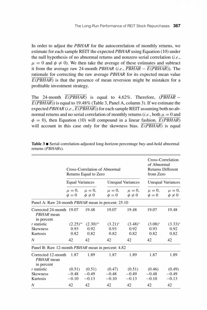
In order to adjust the PBHAR for the autocorrelation of monthly returns, weestimate for each sample REIT the expected PBHAR using Equation (10) underthe null hypothesis of no abnormal returns and nonzero serial correlation (i.e.,µ = 0 and φ �= 0). We then take the average of these estimates and subtractit from the average raw 24-month PBHAR (i.e., PBHAR − E(PBHAR)). Therationale for correcting the raw average PBHAR for its expected mean valueE(PBHAR) is that the presence of mean reversion might be mistaken for aprofitable investment strategy.

The 24-month E(PBHAR) is equal to 4.62%. Therefore, (PBHAR −E(PBHAR)) is equal to 19.48% (Table 3, Panel A, column 3). If we estimate theexpected PBHAR (i.e., E(PBHAR)) for each sample REIT assuming both no ab-normal returns and no serial correlation of monthly returns (i.e., both µ = 0 andφ = 0), then Equation (10) will compound in a linear fashion. E(PBHAR)will account in this case only for the skewness bias. E(PBHAR) is equal

Table 3 � Serial correlation-adjusted long-horizon percentage buy-and-hold abnormalreturns (PBHARs).

Cross-Correlationof Abnormal

Cross-Correlation of Abnormal Returns DifferentReturns Equal to Zero from Zero

Equal Variances Unequal Variances Unequal Variances

µ = 0, µ = 0, µ = 0, µ = 0, µ = 0, µ = 0,φ = 0 φ �= 0 φ = 0 φ �= 0 φ = 0 φ �= 0

Panel A: Raw 24-month PBHAR mean in percent: 25.10

Corrected 24-month 19.07 19.48 19.07 19.48 19.07 19.48PBHAR meanin percent

t statistic (2.25)∗∗ (2.30)∗∗ (3.21)∗ (3.48)∗ (3.08)∗ (3.33)∗

Skewness 0.93 0.92 0.93 0.92 0.93 0.92Kurtosis 0.82 0.82 0.82 0.82 0.82 0.82

N 42 42 42 42 42 42

Panel B: Raw 12-month PBHAR mean in percent: 4.82


t statistic (0.51) (0.51) (0.47) (0.51) (0.46) (0.49)Skewness −0.48 −0.49 −0.48 −0.49 −0.48 −0.49Kurtosis −0.10 −0.13 −0.10 −0.13 −0.10 −0.13

N 42 42 42 42 42 42



Table 3 � continued.




µ = 0, µ = 0, µ = 0, µ = 0, µ = 0, µ = 0,φ = 0 φ �= 0 φ = 0 φ �= 0 φ = 0 φ �= 0

Panel C: Raw 3-month PBHAR mean in percent: 1.91


t statistic (0.69) (0.52) (0.63) (0.49) (0.60) (0.47)Skewness −0.76 −0.84 −0.76 −0.84 −0.76 −0.84Kurtosis −0.15 0.03 −0.15 0.03 −0.15 0.03

N 42 42 42 42 42 42

Note: This table presents results for the serial correlation adjusted percentage buy-and-hold abnormal returns (i.e., average PBHAR – average E(PBHAR)) for the sample ofREITs that announced an open-market stock repurchase program in 1999. Results forthe 24-month, 12-month and 3-month PBHAR are reported, respectively, in Panels A,B and C. PBHAR is the ratio between the BHR on the sample REITs over 24, 12 and3 months after the announcement and the BHR of the average monthly return for theSize/Book-to-Market reference portfolio of non-announcing REITs over the same timeperiod. E(PBHAR) is the expected PBHAR estimated under the hypothesis that µ = 0and φ �= 0 and under the hypothesis that both µ = 0 and φ = 0 . Statistical significanceis assessed using two different assumptions regarding cross-correlation of abnormalreturns. Results in columns 2, 3, 4 and 5 assume that the cross-correlation of abnormalreturn is equal to zero. The traditional Student’s t statistics reported in the second andthird column assume equal variance for the distribution of individual PBHARs. Thet statistics reported in the fourth and fifth column are calculated assuming unequalvariance for the distribution of individual PBHARs. Individual REITs variances areestimated using Equation (11) under the hypothesis that µ = 0 and φ �= 0 as wellas under the hypothesis that both µ = 0 and φ = 0 . Consistently with Fama (1998)and Mitchell and Stafford (2000), the t statistics in the sixth and seventh column arecorrected for the cross-correlation of abnormal returns. Cross-correlations of abnormalreturns are estimated using Equation (13) under the hypothesis that µ = 0 and φ �= 0as well as under the hypothesis that both µ = 0 and φ = 0 .∗Indicates that the mean is different from zero at the 1% level.∗∗Indicates that the mean is different from zero at the 5% level.Cross-sectional t statistics are reported in parentheses.

to 6.03% in this case; therefore, (PBHAR − E(PBHAR)) is equal to 19.07%(Table 3, Panel A, column 2). The difference between E(PBHAR) under thenull hypothesis of no abnormal returns (i.e., µ = 0 and φ �= 0) and E(PBHAR)estimated when both µ = 0 and φ = 0 (i.e., 6.03% − 4.62% = 1.41%) measuresserial correlation or rebalancing bias.



Panels B and C of Table 3 report the results, respectively, for the 12-monthand 3-month PBHARs. The raw average 12-month PBHAR is equal to 4.82%.As for the 24-month performance, we subtract from the raw average PBHARits expected value (i.e., E(PBHAR)) under the null hypothesis of no abnormalreturns (i.e., µ = 0 and φ �= 0) and when both µ = 0 and φ = 0. The correctedaverage 12-month PBHAR is equal to 1.89% under µ = 0 and φ �= 0 and 1.87%when both µ = 0 and φ = 0. Similarly, Panel C in Table 3 reports the results forthe 3-month PBHAR. The raw average is equal to 1.91%. The corrected average3-month PBHAR is equal to 0.89% under µ = 0 and φ �= 0 and 1.18% whenboth µ = 0 and φ = 0. We address the statistical significance of these resultsin the next section.

Hypothesis Tests

Previously, we presented the results for the average PBHARs with and without acorrection for mean reversion. The purpose of this section is to test whether thecorrected PBHAR (i.e., (PBHAR − E(PBHAR))) is statistically different formzero. We test the null hypothesis of no long-run abnormal performance usingthree different measures for the variance of PBHARs.

The Case of Equal Variance

We first assume that Var(PBHARi) = Var(PBHARj) for any i and j firm inthe sample and Cov(PBHARi, PBHARj) = 0 for i �= j . Therefore, under thenull hypothesis of no abnormal returns, (PBHAR − E(PBHAR)) has mean zeroand variance equal to Var(PBHAR)/n, where n is the number of sample firms.The t statistic reported in column 3 of Table 3’s Panel A shows that the cor-rected average 24-month PBHAR is different from zero (i.e., 19.48%) at the5% significance level when E(PBHAR) is estimated assuming µ = 0 andφ �= 0. The evidence does not change when we estimate E(PBHAR) underthe more conservative hypothesis that both µ = 0 and φ = 0. Indeed, theaverage PBHAR is still different from zero (i.e., 19.07%) at the 5% signifi-cance level (Table 3, Panel A, column 2). The t statistics reported in Table 3,columns 2 and 3 of Panels B and C, respectively, for the corrected 12-month and3-month PBHARs suggest that the null hypothesis can never be rejected in thesecases.

Table 4 reports the results for the corrected PBHAR when each observation isweighted according to the size of the share repurchases (weights scaled to sumto one). Evidence in columns 2 and 3 of Panels A, B and C, respectively, forthe corrected 24-month, 12-month and 3-month PBHAR is not different fromthe equally weighted case.



Table 4 � Weighted serial correlation-adjusted long-horizon percentage buy-and-holdabnormal returns (PBHARs).




µ = 0, µ = 0, µ = 0, µ = 0, µ = 0, µ = 0,φ = 0 φ �= 0 φ = 0 φ �= 0 φ = 0 φ �= 0

Panel A: Raw 24-month PBHAR mean in percent: 23.78

Corrected 17.90 18.29 17.90 18.29 17.90 18.2924-month PBHAR

t statistic (2.10)∗∗ (2.14)∗∗ (3.02)∗ (3.31)∗ (2.86)∗ (3.13)∗

Panel B: Raw 12-month PBHAR mean in percent: 4.97


t statistic (0.60) (0.59) (0.53) (0.56) (0.50) (0.53)

Panel C: Raw 3-month PBHAR mean in percent: 2.99


t statistic (1.41) (1.17) (1.21) (1.06) (1.14) (1.00)

Note: This table presents results for the serial correlation adjusted percentage buy-and-hold abnormal returns (i.e., average PBHAR − average E(PBHAR)) for the sample ofREITs (N = 41) that announced an open-market stock repurchase program in 1999.Observations are weighted according to the size of the stock repurchase (weightsscaled to sum to one). Results for the 24-month, 12-month and 3-month PBHAR arereported, respectively, in Panels A, B and C. PBHAR is the ratio between the (BHR)on the sample REITs over 24, 12 and 3 months after the announcement and the BHRof the average monthly return for the Size/Book-to-Market reference portfolio ofnon-announcing REITs over the same time period. E(PBHAR) is the expected PBHARestimated under the hypothesis that µ = 0 and φ �= 0 and under the hypothesis that bothµ = 0 and φ = 0. Statistical significance is assessed using two different assumptionsregarding cross-correlation of abnormal returns. Results in columns 2, 3, 4 and 5assume that the cross-correlation of abnormal return is equal to zero. The traditionalStudent’s t statistics reported in the second and third column assume equal variancefor the distribution of individual PBHARs. The t statistics reported in the fourth andfifth column are calculated assuming unequal variance for the distribution of individualPBHARs. Individual REITs variances are estimated using Equation (11) under thehypothesis that µ = 0 and φ �= 0 as well as under the hypothesis that both µ = 0 and φ= 0. Consistently with Fama (1998) and Mitchell and Stafford (2000), the t statisticsin the sixth and seventh column are corrected for the cross-correlation of abnormalreturns. Cross-correlations of abnormal returns are estimated using Equation (13) underthe hypothesis that µ = 0 and φ �= 0 as well as under the hypothesis that both µ = 0and φ = 0.∗Indicates that the mean is different from zero at the 1% level.∗∗Indicates that the mean is different from zero at the 5% level.



The Case of Unequal Variances

We now assume that Var(PBHARi) �= Var(PBHARj) for any i and j firm inthe sample and Cov(PBHARi, PBHARj) = 0 for i �= j . Therefore, under thenull hypothesis of no abnormal returns, (PBHAR − E(PBHAR) has mean zeroand variance equal to 1

n2

∑ni=1 Var(PBHARi ), where n is the number of sam-

ple firms. Notice that in this case Var(PBHARi) is obtained by estimatingEquation (11) for each REIT for the case when µ = 0 and φ �= 0 and forthe case when both µ = 0 and φ = 0. The t statistic reported in column 5 ofTable 3’s Panel A shows that the corrected average 24-month PBHAR is dif-ferent from zero (i.e., 19.48%) at the 1% significance level when E(PBHAR)is estimated assuming µ = 0 and φ �= 0. The evidence does not change whenwe estimate E(PBHAR) under the more conservative hypothesis that both µ

= 0 and φ = 0. Indeed, the average PBHAR is still different from zero (i.e.,19.07%) at the 1% significance level (Table 3, Panel A, column 4). The t statis-tics reported in Table 3, columns 4 and 5 of Panels B and C, respectively, forthe corrected 12-month and 3-month PBHARs suggest that the null hypothesiscan never be rejected in these cases.


Unequal Variances and Cross-Correlations Different from Zero

Results discussed so far are based on the assumption that the cross-correlation ofPBHARs is equal to zero. Fama (1998) and Mitchell and Stafford (2000) arguethat ignoring a contemporaneous cross-correlation may cause overly rejectingthe null hypothesis of no abnormal returns. Above we provide an estimator forthe contemporaneous covariance for our PBHAR estimator (see Equation (13)).

Assume that Var(PBHARi) �= Var(PBHARj) for any i and j firm in the sampleand Cov(PBHARi, PBHARj) �= 0 for i �= j . Therefore, under the null hy-pothesis of no abnormal returns, the difference (PBHAR − E(PBHAR)) haszero mean and variance equal to 1

n2 [∑n

i=1 Var(PBHARi ) + ∑ni=1 i �= j

∑nj=1 ×

Cov(PBHARi , PBHAR j )]. Notice that in this case Var(PBHARi) andCov(PBHARi, PBHARj) are obtained by estimating, respectively, Equations(11) and (13) for each REIT for the case when µ = 0 and φ �= 0 as well as forthe case when both µ = 0 and φ = 0.

The t statistic reported in column 7 of Table 3’s Panel A shows that correctedaverage 24-month PBHAR is different from zero (i.e., 19.48%) at the 1%



significance level when E(PBHAR) is estimated assuming µ = 0 and φ �=0. The evidence does not change when we estimate E(PBHAR) under the moreconservative hypothesis that both µ = 0 and φ = 0. Indeed, the average PBHARis still different from zero (i.e., 19.07%) at the 1% significance level (Table 3,Panel A, column 6).8 The t statistics reported in Table 3, columns 6 and 7 ofPanels B and C, respectively, for the corrected 12-month and 3-month PBHARssuggest that the null hypothesis can never be rejected in these cases.


BHAR and WRs

We check further robustness of the results reported above by using the tra-ditional BHAR and WR estimators described previously in the article, andwe show that the evidence is consistent with the results obtained with ourPBHAR estimator. The average 24-month BHAR9 for the sample firms is15.56%, which is different from zero at the 5% significance level (Table 5,Panel A, column 4). The interpretation of this result is that buying and holdingsecurities from announcing REITs gives an average return that is 15.56% higherthan the BHAR on the corresponding control sample of non-announcing REITs.The t statistics reported in Table 5, columns 2 and 3 of Panel A, respectively,for the 3-month and 12-month BHARs suggest that the null hypothesis cannotbe rejected in these cases.

Also consistently with the above result, the 24-month wealth relative (WR) isequal to 19.41%, which is different from zero at the 1% significance level(Table 5, Panel B, column 4). The interpretation of this result is that

8 Mitchell and Stafford (2000) are the only ones who propose a direct approximation forthe contemporaneous cross-correlation of abnormal returns. We check if our evidence isalso robust to their approximation of the contemporaneous cross-correlation of abnormalreturns and find that there is still strong evidence against the null hypothesis of noabnormal returns.9 Notice that the performance measure used in this study is not adjusted for the marketbeta. This is consistent with the evidence reported by Ang and Zhang (2002) that themarket loading factor is not relevant in explaining firms’ returns. The average market betais 0.33 for sample REITs and 0.41 for non-sample REITs (Table 1). The implication, ifanything, is that using BHRs without adjusting for beta differences leads to conservativeestimates of the outperformance for the sample of announcing REITs. That is, theevidence reported in this study is robust to adjusting for the market risk.



Table 5 � Buy-and-hold abnormal returns (BHARs) and wealth relative (WR).

Panel A: BHAR

3-Month 12-Month 24-MonthBuy-and-Hold Buy-and-Hold Buy-and-HoldAbnormal Abnormal AbnormalReturns (BHARs) Returns (BHARs) Returns (BHARs)in Percent in Percent in Percent

Mean 2.22 4.87 15.56t statistic (1.39) (1.21) (2.43)∗∗

Skewness −0.60 −0.55 −0.52Kurtosis −0.71 −0.12 1.03

N 42 42 42

Panel B: WR

3-Month Wealth 12-Month Wealth 24-Month WealthRelative (WR) Relative (WR) Relative (WR)in Percent in Percent in Percent

Mean −2.46 5.90 19.41t statistic (1.55) (1.55) (2.96)∗

Skewness −0.54 −0.30 0.67Kurtosis −0.81 −0.19 1.03

N 42 42 42

Note: Panels A and B present respectively results for the BHAR and the WR estimatorsfor the sample of REITs that announced an open-market stock repurchase program in1999. BHAR is the difference between the 3, 12 and 24-month buy-and-hold return(BHR) on the sample REIT and the average BHR on the Size/Book-to-Market referenceportfolio of non-announcing REITs over the same time period. Wealth relative (WR) isthe ratio of the 3, 12 and 24-month buy-and-hold return (BHR) on the sample REIT tothe average BHR on the Size/Book-to-Market reference portfolio of non-announcingREITs over the same time period.∗Indicates that the mean is different from zero at the 1% level.∗∗Indicates that the mean is different from zero at the 5% level.Cross-sectional t statistics are reported in parentheses.

buy-and-hold returns for sample firms are on average 19.41% over and abovethe BHAR on the control sample of non-announcing REITs. The t statisticsreported in Table 5, columns 2 and 3 of Panel B, respectively, for the 3-monthand 12-month WRs suggest that the null hypothesis can never be rejected inthese cases.

Panels A and B of Table 6 report the results for the BHAR and the WR estimatorswhen each observation is weighted according to the size of the share repurchases



Table 6 � Weighted buy-and-hold abnormal returns (BHARs) and wealth relative(WR).

Panel A: BHAR

3-Month 12-Month 24-MonthBuy-and-Hold Buy-and-Hold Buy-and-HoldAbnormal Abnormal AbnormalReturns (BHARs) Returns (BHARs) Returns (BHARs)in Percent in Percent in Percent

Mean 3.13 5.03 13.79t statistic (2.05)∗∗ (1.34) (2.22)∗∗

N 41 41 41

Panel B: WR

3-Month Wealth 12-Month Wealth 24-Month WealthRelative (WR) Relative (WR) Relative (WR)in Percent in Percent in Percent

Mean 3.42 5.84 18.30t statistic (2.23)∗∗ (1.64) (2.75)∗

N 41 41 41

Note: Panels A and B present respectively results for the BHAR and the WR estimatorsfor the sample of REITs that announced an open-market stock repurchase programin 1999. Observations are weighted according to the size of the stock repurchase(weights scaled to sum to one). BHAR is the difference between the 3, 12 and24-month buy-and-hold return (BHR) on the sample REIT and the average BHR on theSize/Book-to-Market reference portfolio of non-announcing REITs over the same timeperiod. Wealth relative (WR) is the ratio of the 3, 12 and 24-month buy-and-hold return(BHR) on the sample REIT to the average BHR on the Size/Book-to-Market referenceportfolio of non-announcing REITs over the same time period.∗Indicates that the mean is different from zero at the 1% level.∗∗Indicates that the mean is different from zero at the 5% level.Cross-sectional t statistics are reported in parentheses.

(weights scaled to sum to one). Evidence is not different from the equallyweighted case.

Why Do REITs Buy Back Their Stock?

The results discussed above suggest that there is compelling evidence that themarket misreacts to open-market stock repurchase announcements by REITs.Both the traditional WR and the PBHAR estimates indicate that the average ab-normal return over a 24-month period is about 19%. The evidence is statisticallysignificant under different specifications for variance and cross-correlation ofabnormal returns, and it is robust to weighting each observation by the size ofthe stock repurchase.



The purpose of this section is to investigate why REITs choose to buy back theirstock. Perhaps management is signaling an expected improvement in future op-erating cash flow. To address this issue we build a measure of long-horizon“abnormal” operating performance (�FFOi) following the event. �FFOi isfunds from operations per share for REIT i over the 2 years following theannouncement minus funds from operations per share in the 2 years endingthe year prior to the announcement. Funds from operations per share quarterlydata are from the SNL Real Estate Securities Quarterly database. If the an-nouncement conveys positive information, then we would expect an increasein the post-announcement “abnormal” operating performance. The average�FFOi in the 2 years following the event is $0.478 per share, which is sta-tistically different from zero at the 5% level. This result implies that stockrepurchase announcements, on average, forecast an improvement in the operat-ing cash flow and provides some support for Jensen’s free cash flow hypothesis.Moreover, consistent with the underreaction hypothesis, this improvement inthe operating performance will be reflected in the market price slowly as re-vealed by the significantly positive evidence of long-horizon market abnormalperformance.

We now investigate the sources of this market underreaction. Undervaluationis a prominent motive for stock repurchases. The undervaluation hypothesisassumes that insiders and outsiders have access to different information sets.Higher information asymmetry implies larger undervaluation. We use Sizei as aproxy for information asymmetry. Information asymmetry is higher for smallerfirms resulting in higher undervaluation. Therefore, we expect a negative rela-tion between PBHARi and Sizei(α1 < 0). Sizei is the natural logarithm of thebook value of total assets (AT , COMPUSTAT data item #6). Past performanceis also used as a proxy for undervaluation. We use the intercept of the marketmodel (Alphai) as a measure of past performance. If REIT managers repur-chase because of poor past performance, then we expect PBHARi and Alphai

to be negatively related (α2 < 0). To obtain Alphai we estimate the followingmarket model using 1 year of CRSP daily data prior to the announcement:Reti,s = αi + βM,i RetM,s + εi,s , where Reti,s is REIT i’s day s rate of returnfrom CRSP and RetM ,s is the market rate of return on day s, as measured bythe CRSP value-weighted portfolio return of all stocks. Dittmar (2000) warnsthat a backward-looking measure of performance, such as Alphai, may not de-tect current undervaluation. Following Ikenberry, Lakonishok and Vermaelen(1995), she suggests that the market-to-book ratio (MBooki) may be a bettermeasure. A low market-to-book ratio would be evidence of undervaluation. Wetherefore expect a negative relation between PBHARi and MBooki (α3 < 0).MBooki is the sum of total debt (DLTT plus DLC, COMPUSTAT data items#9 and #34, respectively), preferred stocks (PSTK, COMPUSTAT data item#130) and market value of equity from COMPUSTAT (MKVAL) over the book



value of total assets (AT , COMPUSTAT data item #6) at the end of the yearprior to the announcement.

If managers do not overinvest (i.e., invest in negative NPV projects), thenthey may use free cash flow to repurchase their own company stock (freecash flow hypothesis) or pay higher dividends. We use �FFOi, PayOuti andLeveri as proxies for the amount of free cash flow. �FFOi is the long-horizon“abnormal” operating performance as defined above. PayOuti is REIT i’s pay-out ratio defined as the ratio of cash dividends (DVC, COMPUSTAT data item#21) to 5% of net income (NI, COMPUSTAT data item #172) plus deprecia-tion, as reported in the SNL Real Estate Securities Quarterly database, at theend of the year prior to the announcement. If managers repurchase more whenfree cash flow is higher, then we can expect PBHARi to be positively relatedto both �FFOi and PayOuti (α4 > 0 and α5 > 0), a forward-looking and abackward-looking measure of free cash flow, respectively. Similarly, managerscould use more debt to repurchase their own stock. Therefore, PBHARi andLeveri should be positively related (α6 > 0). Leveri is the ratio of total bookvalue of long-term debt (DLTT , COMPUSTAT data item #9) to the book valueof total assets (AT , COMPUSTAT data item #6) at the end of the year prior to theannouncement.

The management stock option hypothesis predicts that managers buy backtheir own stock to boost the stock price, and hence the value of their op-tions. Therefore, PBHARi and Optioni should be positively related, (α7 > 0).Optioni is the ratio of the total number of employees’ stock options outstand-ing, as reported in the SNL Real Estate Securities Quarterly database, to thetotal number of shares outstanding from CRSP at the end of the year after theannouncement.

We assess the three above hypotheses using the following regression model:

PBHARi,24 = α0 + α1Sizei + α2Alphai + α3MBooki + α4�FFOi

+ α5PayOuti + α6Leveri + α7Optioni + εi ,

where PBHARi,24 is the PBHAR for REIT i as defined above.

Results are reported in Table 7. Sizei, Alphai and MBooki are all used toaddress the undervaluation hypothesis. The coefficient for Sizei is negativebut not significant. Larger firms are less affected by information asymmetryresulting in less undervaluation. Contrary to expectation, the coefficient for



Table 7 � Stock repurchase motives.

Constant Size Alpha MBook �FFO PayOut Lever Option R2

4.70 −0.19 2.07 −0.52 0.25 0.02 0.32 1.57 0.52(1.96)∗ (−1.62) (1.94)∗ (−3.04)∗∗∗ (2.54)∗∗ (0.78) (0.31) (0.62)

Note: This table presents the results of the estimation of the regression model usedto assess stock repurchase motives for REITs. The independent variable is PBHARi.It is the PBHAR for REIT i measured in the 24 months following the announcement.Sizei is the natural logarithm of the book value of total assets (AT , COMPUSTATdata item #6). Alphai is the intercept obtained from the estimation of the followingmarket model: Reti,s = αi + βM,i RetM,s + εi,s , where Reti,s is REIT i’s day s rate ofreturn from CRSP and RetM ,s is the market rate of return on day s, as measured bythe CRSP value-weighted portfolio return of all stocks. The estimation period is 1year prior to the announcement of the stock repurchase program. MBooki is the sumof total debt (DLTT plus DLC, COMPUSTAT data items #9 and #34, respectively),preferred stocks (PSTK, COMPUSTAT data item #130) and market value of equityfrom COMPUSTAT (MKVAL) over the book value of total assets (AT , COMPUSTATdata item #6) at the end of the year prior to the announcement. �FFOi is fundsfrom operations per share for REIT i over the 2 years following the stock repurchaseannouncement minus funds from operations per share in the 2 years ending the yearprior to the announcement. Funds from operations per share quarterly data are from theSNL Real Estate Securities Quarterly database. PayOuti is the ratio of cash dividends(DVC, COMPUSTAT data item #21) to 5% of net income (NI, COMPUSTAT dataitem # 172) plus depreciation, as reported in the SNL Real Estate Securities Quarterlydatabase, at the end of the year prior to the announcement. Leveri is the ratio of totalbook value of long-term debt (DLTT , COMPUSTAT data item #9) to the book valueof total assets (AT , COMPUSTAT data item #6) at the end of the year prior to theannouncement. Optioni is the ratio of the total number of employees’ stock optionsoutstanding, as reported in the SNL Real Estate Securities Quarterly database, tothe total number of shares outstanding from CRSP at the end of the year after theannouncement.∗Indicates significance at the 10% level.∗∗Indicates significance at the 5% level.∗∗∗Indicates significance at the 1% level.Cross-sectional t statistics are reported in parentheses.

Alphai is positive but only marginally significant, while the coefficient forMBooki is negative and highly significant, which brings strong support forthe undervaluation hypothesis. This evidence is consistent with the univariateresults reported in Panel C of Table 2. There we show that most of the announc-ing REITs (i.e., 76.19%) match with the medium and high book-to-marketreference portfolios of non-announcing REITs. This implies that announc-ing REITs might be better characterized as value firms than non-announcingREITS.



The coefficients for PayOuti and Leveri, as expected, are positive but not sig-nificant. However, the coefficient for �FFOi is positive and highly significant,which shows that managers may repurchase more if they forecast an increasein the free cash flow. This evidence also suggests that the market fully re-flects the quality of the information conveyed by the stock repurchase an-nouncement. Indeed, REITs that experience a sharper increase in the level ofpost-announcement “abnormal” operating performance (�FFO), should alsoexperience a sharper increase in the market price (i.e., PBHAR). Finally, thecoefficient for Optioni is positive, but not significant, and it is inconsistent withthe management stock option hypothesis.

Concluding Remarks

This study investigates whether the market underreacts to open-market stockrepurchase announcements for REITs. We find compelling evidence of long-horizon performance using the traditional BHAR estimator. We notice, however,that the PBHAR estimator may be affected by the serial correlation of monthlyreturns (autocorrelation bias). This problem arises because the bid-ask bounce,discussed by Blume and Stambaugh (1983), can have a different impact onmonthly returns for sample REITs and non-sample REITs. The methodologydeveloped in this study models the serial correlation of monthly excess re-turns and therefore our estimate of expected abnormal returns is free of serial-correlation bias and rebalancing bias.

When we use the autocorrelation bias-free estimator, we still find very strongevidence of long-horizon abnormal performance. Results are robust to differentmeasures of variance of abnormal returns. Following the warning by Fama(1998) and Mitchell and Stafford (2000), we correct the test statistic for thecross-correlation of abnormal returns and still find very strong evidence againstthe null hypothesis of no abnormal returns.

Finally, we investigate whether undervaluation is a motive for the long-horizonabnormal returns. Both univariate and multivariate analyses support the un-dervaluation hypothesis. We also find support for the signaling hypothesis—managers repurchase stock to signal an expected increase in the free cash flow.However, we find no evidence that the repurchases are motivated by executivestock options.

We would like to thank Charles Trzcinka, the editor Thomas G. Thibodeau andan anonymous referee, as well as seminar participants at the University ofConnecticut and the 2003 AREUEA-ASSA Meeting for many helpful commentsand suggestions. We are grateful to Ozcan Sezer for providing the data on stockrepurchase announcements. Any errors are our own.



References

Ali, M. 1977. Analysis of Autoregressive-Moving Average Models: Estimation andPrediction. Biometrika 64: 535–545.Ang, J. and S. Zhang. 2002. Choosing Benchmarks and Test Statistics for Long-HorizonEvent Study. Working Paper. Florida State University: Tallahassee, FL.Banz, R. and W. Breen. 1986. Sample-Dependent Results Using Accounting and MarketData: Some Evidence. Journal of Finance 41: 779–794.Barber, B. and J. Lyon. 1997. Detecting Long-Run Abnormal Stock Returns: The Em-pirical Power and Specification of Test Statistics. Journal of Financial Economics 43:341–372.Blume, M. and R. Stambaugh. 1983. Biases in Computed Returns: An Application tothe Size Effect. Journal of Financial Economics 12: 387–404.Brown, S. and J. Warner. 1985. Using Daily Stock Returns: The Case of Event Studies.Journal of Financial Economics 14: 3–31.Campbell, J., A. Lo and A. MacKinlay. 1997. The Econometrics of Financial Markets.Princeton University Press: Princeton, NJ.Comment, R. and G. Jarrell. 1991. The Relative Signaling Power of Dutch Auction,Fixed Price Tender Offers and Open Market Share Repurchases. Journal of Finance 46:1243–1271.Dann, L. 1981. Common Stock Repurchases: An Analysis of Returns to Bondholdersand Stockholders. Journal of Financial Economics 9: 113–138.Dittmar, A. 2000. Why Do Firms Repurchase Stock? Journal of Business 73(3): 331–355.Fama, E. 1970. Efficient Capital Markets: A Review of Theory and Empirical Work.Journal of Finance 25: 383–417.——. 1998. Market Efficiency, Long-Term Returns, and Behavioral Finance. Journalof Financial Economics 49: 283–306.Howe, K., J. He and G. Wenchi Kao. 1992. One-Time Cash Flow Announcements andFree Cash-Flow Theory: Share Repurchases and Special Dividends. Journal of Finance47: 1963–1975.Ikenberry, D., J. Lakonishok and T. Vermaelen. 1995. The Underreaction to Open MarketShare Repurchases. Journal of Financial Economics 39: 181–208.Isagawa, N. 2002. Open-Market Repurchase Announcements, Actual Repurchases, andStock Price Behavior in Inefficient Markets. Financial Management 31(3): 5–20.Jensen, M. 1986. Agency Costs of Free Cash Flow, Corporate Finance and Takeovers.American Economic Review 76(2): 323–329.Jolls, C. 1998. Stock Repurchases and Incentive Compensation. NBER Working PaperNo. 6467. Cambridge, MA.Kothari, S. and J. Warner. 1997. Measuring Long-Horizon Security Performance. Jour-nal of Financial Economics 43: 301–339.Lang, L. and R. Litzenberger. 1989. Dividend Announcements, Cash Flow Signalingvs. Free Cash Flow Hypothesis. Journal of Financial Economics 24: 181–191.Lewellen, J. 2002. Momentum and Autocorrelation in Stock Returns. Review of Finan-cial Studies 15: 533–563.Loughran, T. and J. Ritter. 2000. Uniformly Least Powerful Tests of Market Efficiency.Journal of Financial Economics 55: 361–389.Lyon, J., B. Barber and C. Tsai. 1999. Improved Methods for Tests of Long-Run Ab-normal Stock Returns. Journal of Finance 54: 165–201.



Mitchell, M. and E. Stafford. 2000. Managerial Decisions and Long-Term Stock PricePerformance. Journal of Business 73: 287–327.Perfect, S., D. Peterson and P. Peterson. 1995. Self-Tender Offers: The Effects of FreeCash Flow, Cash Flow Signaling, and the Measurement of Tobin’s Q. Journal of Bankingand Finance 19: 1005–1023.Ritter, J. 1991. The Long-Run Performance of Initial Public Offerings. Journal of Fi-nancial Economics 46: 3–27.Rubenstein, M. 1976. The Valuation of Uncertain Income Streams and the Pricing OfOption. Bell Journal of Economics 7: 407–425.Sezer, O. 2002. Empirical Investigations on Share Repurchase Programs by Real EstateInvestment Trusts (REITs). Unpublished Ph.D. Dissertation. University of Connecticut:Storrs, CT.Stephens, C. and M. Weisbach. 1998. Actual Share Reacquisitions in Open-MarketRepurchase Programs. Journal of Finance 53: 313–333.Summers, L. 1986. Does the Stock Market Rationally Reflect Fundamental Values?Journal of Finance 41: 591–601.Vermaelen, T. 1981. Common Stock Repurchases and Market Signaling. Journal ofFinancial Economics 9: 139–183.

Documents

The Long-Run Performance of REIT Stock Repurchases