REIT Stock Splits and Liquidity Changes

REIT Stock Splits and Liquidity Changes

Gow-Cheng HuangDepartment of Accounting and Finance

Alabama State UniversityMontgomery, AL 36101-0271

Phone: 334-229-6920E-mail: [email protected]

Kartono LianoDepartment of Finance and Economics

Mississippi State UniversityMississippi State, MS 39762


Ming-Shiun PanDepartment of Finance and Supply Chain Management

Shippensburg UniversityShippensburg, PA 17257


This version: January 2008

1

REIT Stock Splits and Liquidity Changes

Abstract

This study examines whether liquidity improves following REIT stock splits. We find that REIT

liquidity does increase after the announcement of splits. However, the increase in REIT liquidity is

limited in the five-day interval that surrounds the split announcement date. Indeed, after the ex-date, the

liquidity reverts to the level before the split. Our results do not support the view that REIT splits are

made to improve liquidity. Consistent with this result, we also find that changes in liquidity cannot

explain the announcement period abnormal return.

2

1. Introduction

Stock splits appear to be an interesting corporate event to analyze. While stock splits do not

affect a firm’s cash flows, the market tends to react to them positively. The literature suggests that one

main motive for splitting stocks is to realign share prices to an “optimal” trading range (see Lakonishok

and Lev (1987)). Realigning share price may draw more attention to a stock (Grinblatt, Masulis, and

Titman (1984)) and hence lead to an improved liquidity (Muscarella and Vetsuypens (1996)). Indeed, the

survey research by Baker and Powell (1992) reports that moving the stock price into a better trading range

and improving the stock’s liquidity are the primary motives for firms to undertake a split. Theoretically,

Anshuman and Kalay (2002) present a model that shows firms split their stocks to create liquidity. Their

model implies that because of price discreteness related commissions, liquidity traders will time their

trades based on stock price levels. Specifically, liquidity trades may defer their trades until stock prices

drop to lower base levels to save transaction costs. To enhance liquidity, a firm can reset the stock price

to an optimal level by splitting its stock.

Empirically, the evidence that liquidity increases following splits is mixed. While several studies

(Powell and Baker (1993/1994), Schultz (2000), Easley, O’Hara, and Sarr (2001), and Dhar, Goetzmann,

Shepherd, and Zhu (2003)) document an enlarged ownership base after split, other studies (e.g., Conroy,

Harris, and Benet (1990) and Gray, Smith, and Whaley (2003)) show an increase in relative spread after

the split effective date, suggesting that splitting stocks become less liquid following a stock split.

In this paper, we examine liquidity changes following REIT stock splits for the period 1966-2005.

For REITs, drawing attention via splits does not seem important since REIT shares largely are held by

institutional investors (see Lieblich and Pagliari (1997) and Ling and Ryngaert (1997)). Moreover, the

requirement of paying out 90% or 95% of net income as dividends to shareholders in order to avoid

income taxes renders REITs to have less degree of information asymmetry that is typically associated

3

with general stocks.1 Thus, unlike industrial stocks, liquidity may not improve following REIT splits.

Accordingly, we conjecture that to improve liquidity is not a main motive for REIT splits.

Unlike prior studies that examine REIT liquidity in general,2 we focus on how liquidity of REITs

changes following stock splits. Also, unlike prior studies that investigate REIT liquidity via bid-ask

spreads, we consider six liquidity measures because liquidity has various dimensions. Our liquidity

measures represent various dimensions of liquidity including spreads, price impacts, and trading volume.

Additionally, our estimates of liquidity measures require only daily data, rather than intraday data, and

hence we are able to perform our analysis for a much longer time period.

Furthermore, prior studies confine their analysis to liquidity changes after the split effective date.

The impact of splits on liquidity over short periods, especially after announcement dates and before ex-

dates, has not been examined in detail in the literature.3 The two popular stories behind a split decision—

the signaling hypothesis and the target range/improved liquidity hypothesis—appear to have different

implications on trading liquidity of splitting stocks over time. If stock splits convey positive information

content, then we should expect an increase in demand of splitting stocks’ shares. Accordingly, the split

announcement will come with a positive market reaction and an increase in liquidity. In contrast, if the

target range/improved liquidity hypothesis holds, a positive market reaction and improved liquidity may

not occur until the split ex-date when the new stock replaces the unsplit stock in trading. Thus, whether

there is a change in liquidity after the split announcement or after the ex-date has different implications on

the validity of the two hypotheses. To this end, we evaluate various event windows, including the pre-

announcement period, the post-split period, and the post-announcement/pre-split periods—the periods

between the split announcement date and the split’s effective date.

1 The REIT Modernization Act of 1999 reduces the pay-out ratio from 95% to 90%.2 Several studies (e.g., Nelling, Mahoney, Hildebrand, and Goldstein (1995), Below, Kiely, and McIntosh (1996),Bhasin, Cole, and Kiely (1997), Clayton and MacKinnon (2000), and Bertin, Kofman, Michayluk, and Prather(2005)) have examined liquidity of REITs using transaction data.3 Goyenko, Holden, and Ukhov (2005) examine whether liquidity changes after splits in both short- and long-run.However, they focus on monthly liquidity measures and skip the announcement month in their analysis.

4

Using a sample of 48 REIT stock splits for the period 1966-2005, we find abnormal returns in the

five-day window that surrounds the split announcement date. However, no evidence of abnormal returns

is found in the period between the announcement date and the ex date, in the five-day window

surrounding the split ex-date, and in the post-split period. We also find that the sample REIT split firms

exhibit a significant increase in return volatility after the split. Moreover, this post-split increase in return

variance apparently is due to the increase in systematic risk after the split.

More importantly, we find that the REITs experience improved liquidity following stock splits.

This improved liquidity is particularly significant for the five-day announcement period. After the

announcement date but before the ex-date, various liquidity measures appear to decline. After the ex-

date, liquidity has reverted to the level before the split. Our results are robust to various liquidity

measures. Thus, the improved liquidity following REIT stock splits appears to be a short-term

phenomenon that is observed only in the period around the split announcement date. Our results do not

support the view that REIT splits are made to improve liquidity. Consistent with this result, we also find

that changes in liquidity cannot explain the announcement period abnormal return.

The rest of the paper is organized as follows. Section 2 provides a brief literature review on stock

splits. Section 3 describes the various liquidity measures that we use, the data, and abnormal stock

returns around the split announcement and ex-dates of the sample REIT splits. In Section 4, we report

various liquidity measures for the split and matching non-split REITs around the split announcement and

ex-dates. Section 4 also analyzes determinants of the announcement period abnormal returns. Section 5

concludes the paper.

2. Related Research

Stock splits are a puzzling corporate event. While a split does not change a firm’s equity value,

the market tends to react to split announcements favorably. Two hypotheses, the signaling hypothesis and

5

the trading range/liquidity hypothesis, have been proposed to explain the positive excess stock returns that

are associated with stock splits.

The signaling hypothesis suggests that splits are an action made by management to reveal

information about future profitability to the market. Lakonishok and Lev (1987) provide some evidence

that supports the signaling hypothesis. Their analysis shows that split firms exhibit a median growth in

earnings of 16.31 percent in the first post-split year, which is slightly higher than 13.28 percent for their

control sample of non-split firms. However, their major finding leads them to conclude that stock splits

are made mainly to adjust stock prices to “normal” levels. Asquith, Healy, and Palepu (1989) examine

121 stock splits that do not pay dividends prior to or in the announcement year, and report significant

earnings increases several years before the split. McNicholes and Dravid’s (1990) study finds that

analysts’ one-year-ahead earnings forecast errors are positively correlated with announcement abnormal

returns. Ikenberry, Rankine, and Stice (1996) and Desai and Jain (1997) find excess returns in the three

years following a split announcement. Both studies’ results seem to support the view that a split reflects

management’s optimism about the future. Ikenberry et al. also find a negative excess return three years

after the split for a sample of 52 firms that have a negative stock price run-up prior to splits, suggesting

some splits may contain a false signal. The evidence provided in Ikenberry and Ramnath (2002) suggests

that the positive drift in the year following a split announcement is related to market underreaction.

Specifically, they find that financial analysts tend to underestimate splitting firms’ earnings and this

underestimation would gradually decline and approach zero when the actual earnings are announced. In

short, the empirical evidence is somewhat limited to support the claim that stock splits convey favorable

information about future profitability.

With respect to REIT splits, Hardin, Liano, and Huang (2005) find abnormal returns in the

announcement period, but not in the ex-date period or in the long run. Using 45 REIT splits from 1981 to

2001, Li, Sun, and Ong (2006) find that dividend-increasing REITs have smaller market reactions to the

split announcement than those that do not increase dividend prior to the split. Their result implies that

6

dividends and splits for REITs are substitutes of management signals. Further, Li, Sun, and Ong find that

REIT splits provide information on future dividend and leverage changes, which is consistent with the

signaling argument.

Instead of signaling, Grinblatt, Masulis, and Titman (1984) argue that splits can reduce

informational asymmetries by attracting attention paid to a firm. Brennan and Hughes (1991) find that

the number of security analysts following a firm is positively related to the magnitude of stock splits,

which is consistent with the Grinblatt et al. argument. Admati and Pfleiderer (1988) further argue that

splits not only attract informed traders, but also noise traders because of lower post-split share prices.

However, REITs tend to have lower levels of asymmetric information because institutional investors

usually hold large blocks of REIT shares (see Lieblich and Pagliari (1997)). Thus, it is not clear that

REITs would split their shares to draw attention and to reduce informational asymmetry.

Another explanation for stock splits is that firms may prefer their shares to trade within a

particular price range (Copeland (1979)). Management might have this preference because when stock

prices are too high, many small or uninformed investors cannot afford to trade in round lots, thereby

affecting the liquidity of the stock. Splitting shares would improve liquidity by enlarging clientele and

hence reduce the trading cost of the stock (Muscarella and Vetsuypens (1996)).4 Stock split can also

create market liquidity when there are minimum tick size restrictions (Anshuman and Kalay (2002)).

Moreover, management may prefer to bring more small investors, investors who tend not to exercise too

much control, into the firm to create a more controllable ownership mix (Powell and Baker (1993/1994)).

Baker and Gallagher’s (1980) survey reports that 94% of their sample of chief financial officers cited

returning their firm’s share price to an optimal trading range as the main reason for the split. However,

empirical evidence for an improved post-split liquidity is mixed. For instance, several studies (e.g.,

Copeland (1979), Lamoureux and Poon (1987), Conroy, Harris, and Bent (1990), and Dubofsky (1991))

4 Angel (1997) provides another explanation by arguing that splits are to move tick sizes relative to the stock price todesired levels. Angel’s idea is that a large tick size may provide market making firms additional incentives topromote the split stock to small investors. Schultz (2000) finds that there are a lot of small orders, but not largeorders, subsequent to splits, which is consistent with the view that splits act to promote stock trading.

7

find a significant increase in different measures of liquidity, such as stock return volatility or proportional

bid-ask spread. In contrast, Easley, O’Hara, and Saar (2001) find an increase in the number of

uninformed trades, though they also find an increase in the overall trading costs of uninformed traders.

Easley et al. interpret their finding to be consistent with the trading range hypothesis in that stock splits

attract the clientele of small ownership holdings. Dhar et al. (2003) also find individual investors trade

more after stock splits with smaller trade sizes, suggesting improved liquidity.

3. Liquidity Measures, Sample Data, and Control Firm Selection

A. Liquidity Measures

We employ six variables to measure liquidity. These six liquidity variables represent measures

on trade, price impact, and spread. Unlike prior studies that rely on intraday trade and quote data

available from the intraday Trades and Quotes (TAQ) database to estimate bid-ask spreads, we use daily

data to calculate effective spreads. Using the daily data allows us to conduct our analysis for a sample

period as far back as 1962—the year that the CRSP daily database begins, rather than after 1994 when the

TAQ database becomes available. The liquidity measures include the following six variables:

1. Turnover ratio: The turnover ratio is calculated as the average of the daily ratio of trading volume (in

shares) to shares outstanding. Prior studies have used the turnover ratio as a proxy for liquidity

because turnover is negatively correlated with the bid-ask spread.

2. Amihud’s illiquidity ratio, ILLIQ: This illiquidity measure is proposed by Amihud (2002) and is

calculated as d

d

VOLD

R

N

||1, where N is the number of days for which data are available (i.e., trading

volume is not zero), |Rd| is the absolute return on dayd, and VOLDd is dollar trading volume on day d.

As Amihud points out, ILLIQ measures how daily stock price reacts to a dollar of trading volume and

hence is closely related to Kyle’s (1985) concept of illiquidity, defined as the price impact of order

8

flow. Intuitively, a larger trading volume would lead to a small price change. Accordingly, a more

liquid market should be the one with a smaller Amihud illiquidity ratio. Amihud shows that ILLIQ is

strongly positively correlated with illiquidity measures that are calculated from microstructure data.

3. The Amivest liquidity ratio: This liquidity ratio is calculated as ||

1

d

d

R

VOLD

N, where all the terms

are defined as those in the Amihud illiquidity ratio. Just the opposite to the Amihud illiquidity ratio, a

more liquid market should have a larger Amivest liquidity ratio since in a liquid market a larger dollar

trading volume should lead to a small price change.

4. Zeros: This variable is defined as the ratio of the number of days with zero returns to the total

number of trading days. This measure was developed by Lesmond, Ogden, and Trzcinka (1999) as a

proxy for transaction costs, which can be seen as the sum of the spread and commission. They

propose a security model that relates transaction costs to the incidence of zero returns. A key feature

of their model is that marginal investors will not trade or reduce trading if transaction costs exceed the

value of information signal. It is expected that a security with high transaction costs will have more

zero returns and is less liquid than a security with low transaction costs. Thus, one can simply use the

observed incidence of zero returns to infer the liquidity of a security.

5. Dollar spread: Following Holden (2004), we estimate the dollar effective spread (or relative effective

spread) of a security using the time series of daily returns. Holden develops an estimate of the dollar

effective spread that is based on price clustering (see the Appendix for detailed discussions of this

measure). In his model with a fractional tick size, the dollar effective spread can be inferred by

checking the frequency of transactions that occur on odd 1/16s, odd ⅛s, odd ¼s, odd ½s, and whole

dollars. Similarly, for a decimal pricing, the relative effective spread can be inferred by checking the

frequency of transactions that occur on off pennies, off nickels, off dimes, off half dollars, and whole

dollars. Note that his estimation of relative effective spread does not require continuously quoted bid-

ask spreads and instead requires only time series of security daily returns. Consequently, we are able

to perform our analysis for time periods that intraday data (e.g., the TAQ database) are not available.

9

6. Effective spread: The effective spread is calculated by dividing the dollar spread with the average

daily trading price. Goyenko, Holden, Lundblad, and Trzcinka (2005) sample various proxies for

liquidity based on daily data and compare them with those calculated from the TAQ database. They

find that Holden’s effective spread and price impact proxies are the best monthly liquidity measures.

B. Sample Data

The data for real estate investment trusts (REITs) with SIC code 6798 or share codes 18 (ordinary

common shares, REITs) or 48 (shares of beneficial interest, REITs) are retrieved from the Center for

Research in Security Prices (CRSP) NYSE, AMEX, and NASDAQ files. To be included in the sample, a

REIT has to meet the following criteria: (1) it announced a stock split (the distribution code is 5523 in

CRSP); (2) the split factor (the code is facshr in CRSP) is at least 0.25, which is equivalent to a 5-for-4

split; and (3) at least 60% of daily stock prices, trading volume, and return data are available in the CRSP

daily return file from 122 days prior to the split announcement date to 122 days after the split effective

date. We also require a REIT to wait for one year before it can reenter the sample to avoid dependence in

overlapping data.

Consistent with Hardin, Liano, and Huang (2005) and Li, Sun, and Ong (2006), REITs rarely split

their shares. Our final sample consists of 48 REIT stock split announcements made during the period

1966-2005. Specifically, there are 3 splits before 1980, 18 splits in the 1980s, 17 splits in the 1990s, and

10 splits after 2000. Table 1 reports the number of REIT stock splits by split ratio. Similar to the stock

split literature, our results show that certain split ratios are more common than others. About 35 percent

(17 splits) of the sample have a 2-for-1 split; another 50 percent (24 splits) are for a 3-for-2 split.

Table 1 also reports the price run-up before the split and the cumulative abnormal returns

(calculated as the return difference between the sample REITs and a REIT equally-weighted index) for

various windows. The mean (median) price run-up, which is the price run-up from 122 trading days

before the split announcement to 5 trading days prior to the split, is 18.79% (15.85%). Considering that

10

REITs are income oriented investments that offer a relatively high quarterly dividend yield of 2.07% (see

Hardin, Liano, and Huang (2002)), the 18.79% price appreciation in six months indicates that most REITs

exercise a stock split when the stock has a reasonable price run-up. The mean (median) cumulative

market-adjusted abnormal return during days –2 to +2 relative to the split announcement is 2.99%

(3.37%), indicating a favorable market reaction to the REIT split announcement. The positive market

reaction suggests that splits lead to a higher demand by investors. This greater demand in split REITs’

shares could be due to some sort of information content in signaling, a more “affordable” share price, or

both. Either case, the higher demand should lead to improved trading liquidity.

Our sample split REITs experience a mean (median) cumulative abnormal return of −0.10%

(0.32%) during the period from 3 days after the announcement (a+3) to 3 days before the ex-date (e−3).

Nayar and Rozeff (2001) point out that trading unsplit or pre-split shares prior to the split ex-date is

inconvenient because of frictions associated with the delivery of split shares and the settlement of a due

bill that the sellers provide to the buyers. Thus, investors are reluctant to buying shares after the record

date and before the ex-date. Consequently, prices are depressed during the announcement-to-ex-date

period and the negative abnormal return likely reflects this phenomenon.

Unlike non-REIT splits,5 we find insignificant abnormal returns during the 5-day ex-date period

(e−2 to e+2). The mean (median) abnormal return during this period is negative (though insignificant) of

−0.27% (−1.01%). This result suggests that the disappearance of inconvenience of trading unsplit REIT

shares around the ex-date is not that significant. Or it could mean that brokers do not promote REIT

shares to investors, especially small investors, as the broker promotion theory suggests.

5 The previous literature documents positive abnormal returns surrounding the split ex date. Nayar and Rozeff(2001) argue that the positive ex-date abnormal returns following regular stock splits is due to the inconvenience oftrading unsplit shares, leading to declines in stock prices near record dates and then followed by price increases atex-dates. On the other hand, Kadapakkam, Krishnamurthy, and Tse (2005) suggest that the positive ex-dateabnormal return is related to an increased in intensity of small investor buying near ex-dates, which is due tobrokers’ promotion of splitting stocks to small investors. Both the trading inconvenience and the broker promotionhypothesis suggest the existence of an ex-date effect.

11

The broker promotion hypothesis also implies that larger relative spreads after splits will induce

brokers to promote shares to small investors. If this is the case, abnormal returns might continue after ex-

date. We find a negative (though not significant) cumulative return in the eight-day post-split interval

(e+3 to e+10) (see Table 1). Our results are therefore not consistent with the broker promotion

hypothesis.

We also examine abnormal returns for a longer term interval (e+3 to e+122). Consist with

Hardin, Liano, and Huang (2005), we do not find a long-term price appreciation following REIT splits.

In short, abnormal returns exist only in a very short-term window surrounding the REIT split

announcement date. No evidence of abnormal returns is found in the period between the announcement

and ex dates, in a short-term window surrounding the ex date, and in short- and long-term post-split

periods.

C. Control Firm Selection

To evaluate whether or not REIT liquidity improves after stock splits, we use a matching firm

approach. Our selection of matching REITs is based on the exchange, share price, and trading liquidity.

Our intention is to select matching REITs that do not split but have similar pre-split share price and

liquidity as the sample REITs. Specifically, for each split REIT, we select matching REITs that do not

split over a one-year period prior to the split REIT’s announcement date using the following criteria: (1)

REITs that are from the same exchange and (2) the share price is within ±10% of the split REIT’s share

price three trading days prior to the split announcement. From the REITs that meet these two

characteristics, we choose the REIT that has the closest Amihud’s illiquidity ratio for the six months

before the split announcement (a−122 to a−5). Just like the sample REITs, we require the daily CRSP

database to contain information on the matching REITs’ stock prices, trading volume, and returns for six

months around the split announcement date.

12

4. Empirical Results

A. Changes in Liquidity

If splits convey positive information on future profitability of REITs to the market, then trading

liquidity of the split REIT’s stock share should increase after the split announcement because investors

have more desire to buy the stock. On the other hand, if returning the share price to a target range and

improving liquidity are the primary purpose of the split, then liquidity likely will not increase before the

split effective date because before this date all trading are in the unsplit shares. Moreover, the

inconvenience of trading unsplit shares before the ex date may delay the purchase from investors until the

ex-date. To determine whether or not liquidity of split REITs improves after splits, we calculate the six

liquidity measures described above for the split REITs for six windows, including the pre-split (a−122 to

a−3), the announcement (a−2 to a+2), the announcement-to-ex-date (a+3 to e−3), the ex-date (e−2 to

e+2), the short-term post-ex (e+3 to e+10), and the long-term post-ex (e+3 to e+122) periods. These six

intervals span about a one-year window around the split announcement and ex dates. We then determine

whether liquidity improves by evaluating how liquidity measures change over the six intervals.

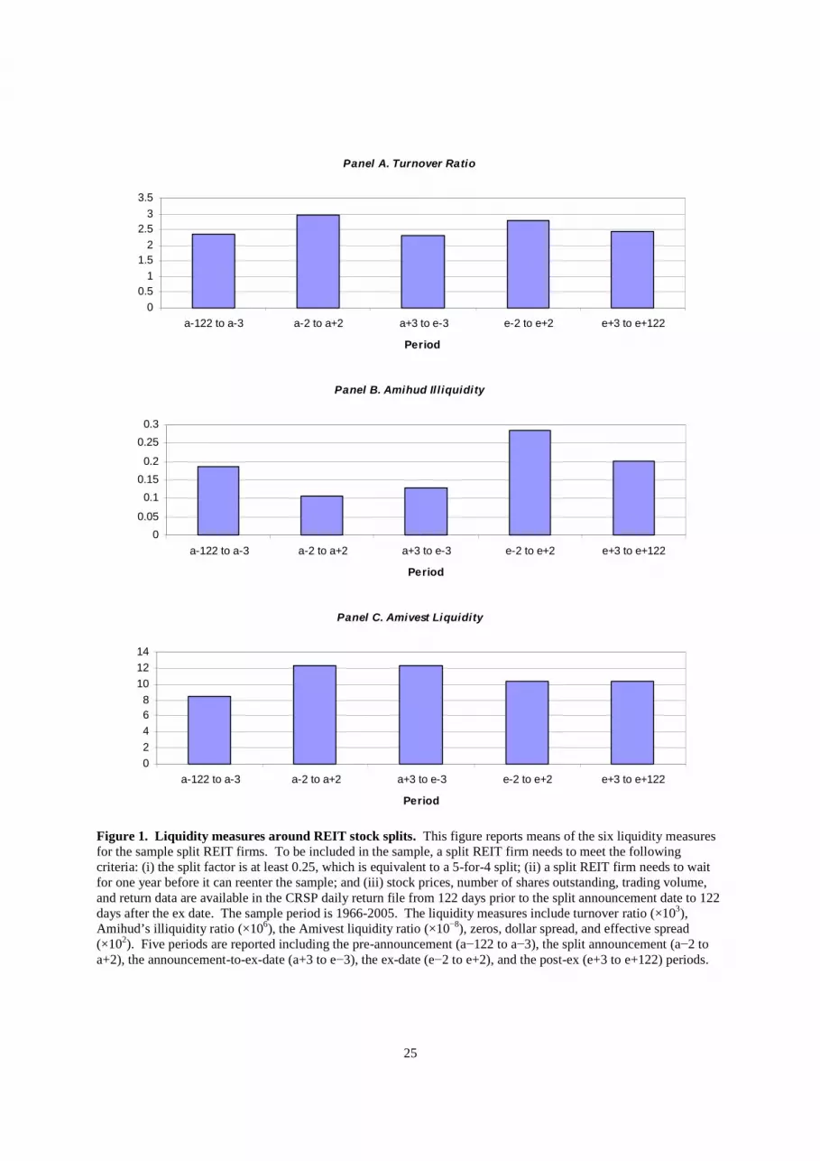
Figure 1 plots the means of the six liquidity measures for the six periods. It appears that except

the dollar spread, the various measures show an improvement in liquidity after the split announcement.

But this improvement in liquidity also appears to disappear gradually over the subsequent intervals after

the announcement.

Table 2 shows the six liquidity measures for the six windows. Panel A shows that the turnover

ratio of the split REITs increases from the pre-split period to the announcement period and then declines

over the subsequent four periods, with the turnover ratio in the long–term post-ex period reverts to the

level as in the pre-announcement period. Specifically, the mean (median) turnover ratio increases from

2.360 × 1,000−1 (1.951 × 1,000−1) in the pre-split period to 2.964 × 1,000−1 (2.436 × 1,000−1) in the

13

announcement period. After the announcement, the mean (median) falls to 2.312 × 1,000−1 (1.750 ×

1,000−1) in the announcement-to-ex period, which could reflect the inconvenience of trading unsplit share

during this period. The mean (median) turnover ratio then increases to 2.795 × 1,000−1 (2.088 × 1,000−1)

in the ex-date period, but subsequently declines to 2.539 × 1,000−1 (1.895× 1,000−1) in the seven-day post-

ex period and to 2.438 × 1,000−1 (2.010 × 1,000−1) in the 120-day post-ex period. The peak of turnover

ratio at the split announcement period may reflect the optimism on firm’s operating performance (see Li,

Sun, and Ong (2006)) shared by investors. Thus, REIT stock splits appear to increase the trading

turnover, especially in the period between the announcement and effective dates.

Table 2, Panel B shows the sample REITs’ Amihud illiquidity ratios,6 which measure price

impact of order flow. The Amihud illiquidity ratios follow a similar trend over time as the turnover

ratios. The mean (median) Amihud illiquidity ratio declines from 0.185 (0.020) in the six-month pre-split

period to 0.107 (0.016) in the five-day announcement period and then increases to 0.202 (0.027) in the

six-month post-ex period. Similar to the turnover ratio, the Amihud illiquidity ratio suggests poor

liquidity for split REITs during the period between the announcement and the ex-dates when compared to

the announcement period. After the ex-date, the split REIT’s trading liquidity as measured by the

Amihud illiquidity ratio seems to revert back to a level that is even higher than that prior to the split.

Panel C of Table 2 reports the Amivest liquidity ratios. Similar to the previous two liquidity

measures, the Amivest liquidity ratios increase from the pre-split period to the announcement period and

then decline over the subsequent four periods. The Amivest liquidity ratio also indicates that liquidity

improves around the announcement date.

In Panel D of Table 2, we report the proportion of days with zero returns, which is to proxy for

transaction costs as proposed by Lesmond et al. (1999). After the split, this measure suggests that

liquidity has improved, given that the mean (median) declines from 16.7% (16.7%) of zero returns prior

to the split to 10.0% (0%) during the announcement date. The ex-date period also shows low percentage

6 All the Amihud illiquidity figures are multiplied by 106.

14

of zero returns relative to other windows. After the ex date, the percentage of trading days with zero

returns appears to revert back to the pre-split level if not higher.

Panels E and F of Table 2 show the dollar effective and relative spreads, respectively. Unlike

other liquidity measures, the ex-date period shows the highest liquidity with the smallest dollar spread of

$0.163. In the post-ex period, the dollar effective spread increases to $0.225 and is slightly larger than its

pre-split level of $0.218. In contrast, the relative spreads show a different story. The relative spread

increases from the pre-split level of 0.447 percent to 0.625 percent in the ex-date period—the highest.

The relative spread remains high at about 0.621 percent during the 6-month period after the ex date. This

finding that relative spreads increase after splits become effective is consistent with the stock split

literature that focuses on general stocks (e.g., Lamoureux and Poon (1987), Conroy et al. (1990), and

Gray et al. (2003)).

To further evaluate whether the sample split REITs’ liquidity improves after the split, we

compare the split REITs’ liquidity measures to those of the matched non-split REITs. The matched non-

split REITs’ liquidity measures are also reported in Table 2. We test statistical significance of the mean

(median) differences of liquidity measures using a t-statistic (the Wilcoxon signed rank test). The results

are somewhat mixed. While some liquidity measures (e.g., turnover ratio, Amihud illiquidity, and Zeros)

indicate that the sample split REITs are less liquid than the matched REITs over various time intervals,

others (e.g., Amivest liquidity) show that the sample split REITs are more liquid. Nevertheless,

statistically speaking, the sample split REITs have similar liquidity as the matched REITs, except during

the post-ex period based on the Zeros and effective spreads. Thus, stock splits appear not to affect

REITs’ liquidity, relative to their peers.

B. Changes in Risk

15

Prior studies (e.g., Lamoureux and Poon (1987), Dubofsky (1991), and Desai et al. (1998))

document that return volatility increases following the split ex date. Several studies (e.g., Desai et al.

(1998) and Easley et al. (2001)) attribute the post-split volatility increase to increase in spreads of split

firms. In the previous sub-section, we find that the relative spreads of split REITs do increase after the

split becomes effective. Alternatively, the increase in volatility could be caused by an increase in either

equity beta or residual return variance.

In this study, we also analyze changes in REIT return variance and its systematic and

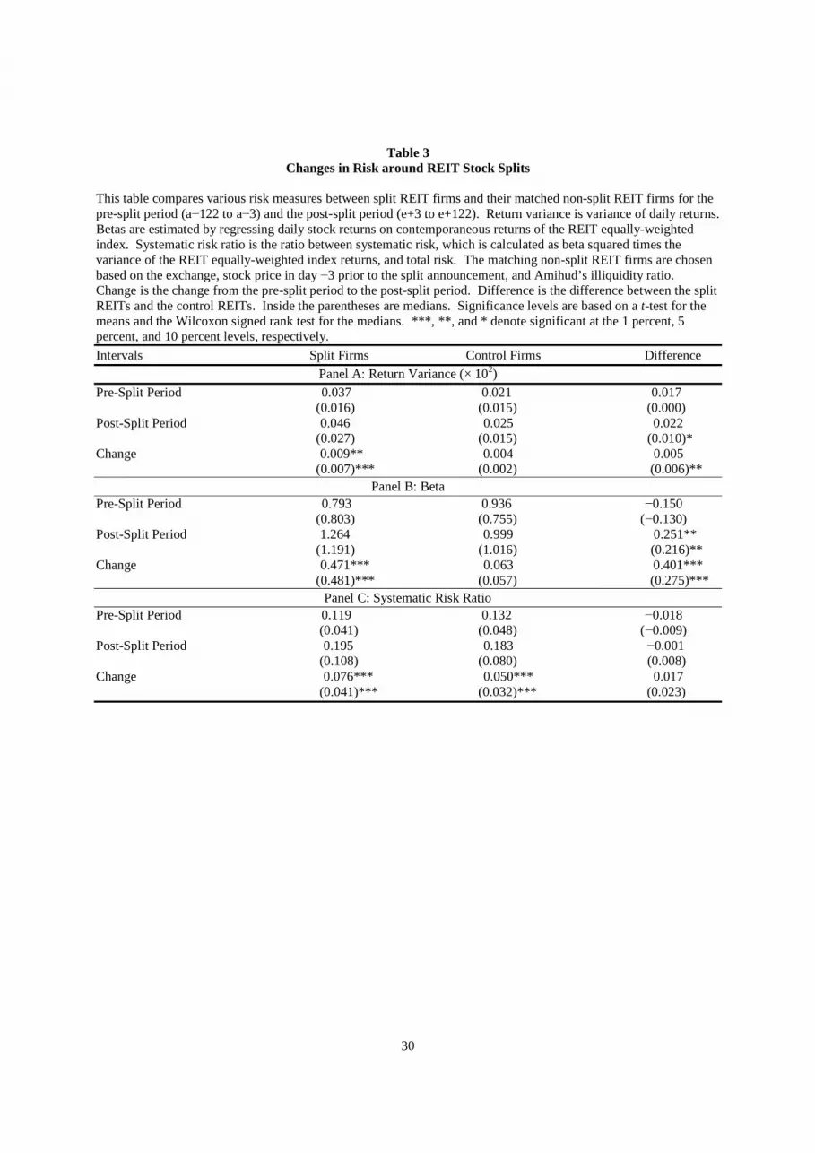
unsystematic components to investigate the sources of volatility changes following splits. Table 3

contains various risk measures for two windows, including a 6-month period prior to the split

announcement date (a−122 to a−3) and a 6-month period after the ex date (e+3 to e+122). In the pre-split

period, the mean (median) daily return variance for the split REITs is 0.037% (0.016%), which is larger

(though not significant) than 0.021% (0.015%) for the matched non-split REITs (see Panel A). After the

split, the mean (median) return variance of the split REITs increases by 0.009% (0.011%) to 0.046%

(0.027%), while the mean (median) return variance of the matched non-split REITs increases by 0.004%

(0%) to 0.025% (0.015%). Although the mean difference in the return variances between the split and

non-split REITs after the split is insignificant, the median difference is marginally significant. Thus,

similar to non-REIT firms, our results indicate that after the split, the total risk of split REITs not only

increases but also increases at a larger amount relative to REITs that do not split.

Table 3, Panel B reports beta estimates.7 Similar to total risk, the equity beta of the split REITs

increases after the split.8 Specifically, the mean (median) beta value increases from 0.793 (0.803) before

the split to 1.264 (1.191) after the split. Although the split REITs have smaller systematic risk than their

matched non-split peers before the split, they exhibit significantly higher systematic risk after the split.

Panel C shows that the split REITs also experience an increase in systematic risk ratio, which is the ratio

7 Betas are estimated by regressing REIT daily stock returns on contemporaneous returns of the REIT equally-weighted index.8 Chiang, Lee, and Wisen (2004) find that the beta of REITs fluctuates depending on market conditions and businesscycles.

16

between systematic risk (calculated as beta squared times the variance of the REIT equally-weighted

index returns) and total risk. Our result shows that the systematic risk of split REITs accounts for only

11.9% of the total risk before the split. The systematic risk ratio, however, increases to 19.5% after the

split. Similar to the beta result, while the split REITs have smaller systematic risk ratio than the matched

REITs in the pre-split period, they have higher systematic risk ratio after the split. Overall, our findings

in Table 3 suggest that the post-split increase in split REIT return variance is due to the increase in

systematic risk after the split.

C. Abnormal Returns and Changes in Liquidity

Another analysis that we perform is evaluating determinants of the announcement period

abnormal returns. To this end, we employ a regression analysis. Our main purpose here is to see whether

the positive market reaction to REIT split announcements reported above can be explained by the

improved liquidity. Specifically, we regress the 5-day cumulative abnormal returns in the announcement

period on liquidity measures and some control variables. The regression model is:

CARi = 0 + 1ILLIQi + 2PO_PRICEi + 3VOLAi + 4INTFi + i. (1)

CAR is the 5-day (a−2 to a+2) announcement period abnormal return as reported in Table 1. ILLIQ is

the change in the Amihud illiquidity ratios between the pre-announcement period and the announcement

period,9 of which a negative change means an increase in liquidity. The improved liquidity hypothesis

suggests that the coefficient of ILLIQ should be negative. PO_PRICE is share price after the split and is

calculated as the share price five trading days before the split divided by (1 + split factor). If the primary

motivation behind a split is to return the REIT’s share price to a lower range, we should observe a

negative coefficient for PO_PRICE, meaning that the market reacts more positively to lower price after

the split. VOLA is the change in systematic risk ratio between the pre-split period and the post-split

9 Similar results are obtained when other liquidity measures are used and hence are not reported to save space.

17

period as reported in Table 3, Panel C. We use return volatility to proxy for the stock price elasticity of

demand.10 Since the abnormal return is positive, we expect ΔVOLA to have a positive relation with the

abnormal return. INTF is a dummy variable with a value of 0 for non-integer splits (e.g., 5 for 4) and a

value of 1 for integer splits (e.g., 2 for 1). The INTF dummy variable is to capture the case that non-

integer splits will result a round lot holder of 100 shares to receive a fraction of a round lot. In the case

that investors prefer holding round lots, then abnormal return should be smaller for non-integer splits. If

this relation holds, then CAR in the announcement period will be positively related to INTF.

The results reported in Table 4 show that the announcement period abnormal return is not

significantly related to the dependent variables. The estimated coefficient of ΔILLIQ is negative but is

insignificant, suggesting that the positive market reaction cannot be explained by the improved liquidity.

As expected, the split announcement is negatively (albeit insignificantly) related to the post-split stock

price. ΔVOLA is positive, meaning that stocks with higher variance tend to have higher returns. INTF is

negative, indicating that some investors may not avoid trading stocks with non-integer splits.

Previous REIT literature suggests that there might be a structural change in the REIT industry in

the early 1990s. Chan, Leung, and Wang (1998) document a substantial increase in investment in REITs

by institutional investors after 1990. Gentry, Kemsley, and Mayer (2003) find that REITs received more

analyst coverage since the REIT boom that began in the early 1990s. The increased institutional

involvement and increased analyst coverage likely will gain in liquidity and trading volume. To capture

this structural change, we therefore include in our regression another dummy variable with a value of 1 if

the split is announced before 1990, and 0 otherwise. We also include an interaction variable that is equal

to the value of ΔILLIQ if the split announcement year is before 1990, and 0 otherwise. If the REIT

market is less liquid before 1990 and splits made before 1990 are to improve REIT liquidity, the

coefficient of the interaction variable should be negative. However, we yield a positive coefficient (not

10 Hodrick (1999) suggests that return volatility is a good measure of the stock price elasticity of demand (defined asthe percentage change in quantity demanded given a percentage change in price). He finds that higher returnvolatility is associated with higher elasticity.

18

reported). This result suggests that even for a period during which the REIT market is not so liquid, the

change in liquidity cannot explain the positive market reaction to splits.

5. Conclusion

In this study, we examine whether liquidity improves following REIT splits. Using a sample of

48 REIT stock splits over the period 1966-2005, we find that most liquidity measures increase following

stock splits. However, this improved liquidity is limited to the five-day interval that surrounds the split

announcement date. After the announcement date but before the ex-date, our liquidity measures appear to

decline. Following the ex-date, liquidity has reverted to the level before the split. Our results imply that

to improve trading liquidity is not a motive of REIT splits. Consistent with this implication, we also find

that changes in liquidity cannot explain the split announcement effect. Moreover, we find significant

increase in return volatility after the split. This post-split increase in return variance apparently is due to

the increase in systematic risk after the split.

19

Appendix

This appendix presents the method developed by Holden (2004) for the purpose of estimating

effective spreads using daily data. Holden develops an estimate of the effective spread that is based on

price clustering. His method of calculating the effective spread does not require intraday data and hence

allows researchers to estimate spread measures going back to 1962—the year that the CRSP daily

database begins. The effective spread models assumes that each day the effective spread jumps randomly

among multiple spread sizes and that each spread size leads to a daily trade price based on corresponding

round increments. For instance, on a fractional price grid the effective spread might jump each day

between $1/16, $⅛, $¼, $½, and $1. When the spread is $1/16, then each of the sixteen price increments

($1/16, $⅛, $3/16, . . . , $15/16, and $1) are equally likely. When the spread is $⅛, then each of the eight

rounder price increments ($⅛, $¼, $⅜, . . ., $⅞, and $1) is assumed to happen equally likely and odd

1/16s are not used. Thus, one can observe the frequency of odd 1/16 prices to infer the probability of a

$1/16 spread. The probability of a $⅛ spread can be inferred by observing the difference in frequency

between odd ⅛s and odd 1/16s. And so on.

The details of calculating the effective spread can be described by considering a factional price

grid with a minimum tick size of $1/16. Let N(odd 1/16s), N(odd ⅛s), N(odd ¼s), N(odd ½s), and

N(wholes) be the number of odd 1/16 prices, the number odd ⅛ prices, the number of odd ¼ prices, the

number of odd ½ prices, and the number of whole dollar prices, respectively. The probability of each

price cluster can be calculated as

Pr(Odd 1/16s) = N(odd 1/16s)/N(Positive),

Pr(Odd ⅛s) = N(odd ⅛s)/N(Positive),

Pr(Odd ¼s) = N(odd ¼s)/N(Positive),

Pr(Odd ½s) = N(odd ½s)/N(Positive), and

Pr(Wholes) = N(Wholes)/N(Positive),

where N(Positive) is the number of positive volume days.

20

Next step is to calculate the inferred probability of each spread size from the price cluster

probabilities. That is,

Pr(1/16 Spread) = Min[2· Pr(Odd 1/16s), 1],

Pr(⅛ Spread) = Min[Max{2· Pr(Odd ⅛s) − Pr(Odd 1/16s), 0}, 1 − Pr(1/16 Spread)],

Pr(¼ Spread) = Min[Max{2· Pr(Odd ¼s) − Pr(Odd ⅛s), 0}, 1 − Pr(1/16 Spread) − Pr(⅛ Spread)],

Pr(½ Spread) = Min[Max{2· Pr(Odd ½s) − Pr(Odd ¼s), 0}, 1 − Pr(1/16 Spread) − Pr(⅛ Spread) −

Pr(¼ Spread)],

Pr(1 Spread) = Min[Max{2· Pr(Wholes) − Pr(Odd ½s), 0}, 1 − Pr(1/16 Spread) − Pr(⅛ Spread) −

Pr(¼ Spread) − Pr(½ Spread)].

Given the inferred probability of each spread size, our fifth liquidity measure, the dollar spread

(or the dollar effective tick) can be calculated as a weighted average of each spread size

Dollar Spread = Pr(1/16 Spread)·(1/16) + Pr(⅛ Spread)·(⅛) + Pr(¼ Spread)·(¼) + Pr(½ Spread)·(½) +

Pr(1 Spread)·(1).

Our sixth liquidity measure, the effective spread can be calculated as

Effective Spread = Dollar Spread/Price,

where Price is average daily trading price.

21

References

Admati, A. R., and P. Pfleiderer, 1988, “A theory of intraday patterns: volume and price variability,”

Review of Financial Studies 1, 3-40.

Amihud, Y., 2002, “Illiquidity and stock returns: cross-section and time-series effects,” Journal of

Financial Markets 5, 31-56.

Angel, J. J., 1997, “Tick size, share prices and stock splits,” Journal of Finance 52, 655-681.

Anshuman, V. R., and A. Kalay, 2002, “Can splits create market liquidity? theory and evidence,” Journal

of Financial Markets 5, 83-125.

Asquith, O., P. Healy, and K. Palepu, 1989, “Earnings and stock splits,” Accounting Review 64, 387-403.

Baker, H. K., and P. L. Gallagher, 1980, “Management’s view of stock splits,” Financial Management 9,

73-77.

Baker, H. K., and G. E. Powell, 1992, “Why companies issue stock splits,” Financial Management 21,

11.

Bhasin, V., R. A. Cole, and J. K. Kiely, 1997, “Changes in REIT liquidity 1990-1994: Evidence from

intra-day transactions,” Real Estate Economics 25, 615-630.

Below, S. D., J. K. Kiely, and W. McIntosh, 1996, “REIT pricing efficiency; Should investors still be

concerned,” Journal of Real Estate Research 12, 397-412.

Bertin, W., P. Kofman, D. Michayluk, and L. Prather, 2005, “Intraday REIT liquidity,” Journal of Real

Estate Research 27, 155-176.

Brennan, M. J., and P. J. Hughes, 1991, “Stock prices and the supply of information,” Journal of Finance

46, 1665-1691.

Chan, S. H., W. K. Leung, and K. Wang, 1998, “Institutional investment in REITs: Evidence and

implications,” Journal of Real Estate Research 16, 357-374.

Chiang, K. C. H., M. L. Lee, and C. H. Wisen, 2004, “Another look at the asymmetric REIT-beta puzzle,”

Journal of Real Estate Research 26, 25-42.

22

Clayton, J. and G. MacKinnon, 2000, “Measuring and explaining changes in REIT liquidity: Moving

beyond the bid-ask spread,” Real Estate Economics 28, 89-115.

Conroy, J. S., R. S. Harris, and B. A. Benet, 1990, “The effects of stock splits on bid-ask spreads,”

Journal of Finance 45, 1285-1295.

Copeland, T. E., 1979, “Liquidity changes following stock splits,” Journal of Finance 34, 115-141.

Desai, A. S., M. Nimalendran, and S. Venkataraman, 1998, “Changes in trading activity following stock

splits and their effect on volatility and the adverse-information component of the bid-ask spread,”

Journal of Financial Research 21, 159-183.

Desai, H., and P. C. Jain, 1997, “Long-run common stock returns following stock splits and reverse

splits,” Journal of Business 70, 409-433,

Dhar, R., W. N. Goetzmann, S. Shepherd, and N. Zhu, 2003, “The impact of clientele changes: Evidence

from stock splits,” working paper, Yale University.

Dubofsky, D. A., 1991, “Volatility increases subsequent to NYSE and AMEX stock splits,” Journal of

Finance 46, 421-431.

Easley, D., M. O’Hara, and G. Saar, 2001, “How stock splits affect trading: a microstructure approach,”

Journal of Financial and Quantitative Analysis 36, 25-51.

Gentry, W. M., D. Kemsley, and C. J. Mayer, 2003, “Dividend taxes and share prices: Evidence from

Real Estate Investment Trusts,” Journal of Finance 58, 261-282.

Goyenko R. Y., C. W. Holden, C. T. Lundblad, and C. A. Trzcinka, 2005, “Horseraces of monthly and

annual liquidity measures,” working paper, Indiana University.

Goyenko R. Y., C. W. Holden, and A. D. Ukhov, 2005, “Do stock splits improve liquidity?” working

paper, Indiana University.

Gray, S. F., T. Smith, and R. E. Whaley, 2003, “Stock splits: implications for investor trading costs,”

Journal of Empirical Finance 10, 271-303.

Grinblatt, M. S., R. W. Masulis, and S. Titman, 1984, “The valuation effects of stock splits and stock

dividends,” Journal of Financial Economics 13, 461-490.

23

Hardin III, W. G., K. Liano, and G. C. Huang, 2002, “The ex-dividend pricing of REITs,” Real Estate

Economics 30, 533-549.

Hardin III, W. G., K. Liano, and G. C. Huang, 2005, “REIT stock splits and market efficiency,” Journal

of Real Estate Finance and Economics 30, 297-315.

Hodrick, L. S., 1999, “Does stock price elasticity affect corporate financial decisions?” Journal of

Financial Economics 52, 225-256.

Holden, C. W., 2004, “Low frequency measures of liquidity and spread components,” working paper,

Indiana University.

Ikenberry, D. L., G. Rankine, and E. K. Stice, 1996, “What do stock splits really signal?” Journal of

Financial and Quantitative Analysis 31, 357-375.

Ikenberry, D. L. and S. Ramnath, 2002, “Underreaction to self-selected news events: the case of stock

split,” Review of Financial Studies 15, 489-526.

Kadapakkam, P.-R., S. Krishnamurthy, and Y. Tse, 2005, “Stock splits, broker promotion, and

decimalization,” Journal of Financial and Quantitative Analysis 40, 873-895.

Kyle, A. S., 1985, “Continuous auctions and insider trading,” Econometrica 53, 1315-1335.

Lakonishok, J. and B. Lev, 1987, “Stock splits and stock dividends: why, who, and when,” Journal of

Finance 42, 913-932.

Lamoureux, C. G. and P. Poon, 1987, “The market reaction to stock splits,” Journal of Finance 42, 1347-

1370.

Lesmond, D. A., J. P. Ogden, and C. A. Trzcinka, 1999, “A new estimate of transaction costs,” Review of

Financial Studies 12, 1113-1141.

Li, Q., H. Sun, and S. E. Ong, 2006, “REIT splits and dividend changes: Tests of signaling and

information substitutability,” Journal of Real Estate Finance and Economics 33, 127-150.

Lieblich, F. and J. Pagliari, Jr., 1997, “REITs: A look at institutional interest,” Illinois Real Estate Letter,

University of Illinois at Urbana-Champaign, Summer Issue.

24

Ling, D. and M. Ryngaert, 1997, “Valuation uncertainty, institutional involvement, and the underpricing

of IPOs: The case of REITs,” Journal of Financial Economics 43, 433-456.

McNichols, M. and A. Dravid, 1990, “Stock dividends, stock splits, and signaling,” Journal of Finance

45, 857-879.

Muscarella, C., and M. Vetsuypens, 1996, “Stock splits: signaling or liquidity? the case of ADR ‘solo

splits’,” Journal of Financial Economics 42, 3-26.

Nayar, N. and M. S. Rozeff, 2001, “Record date, when issued and ex date effects in stock splits,” Journal

of Financial and Quantitative Analysis 36, 119-139.

Nelling, E. F., J. M. Mahoney, T. L. Hildebrand, and M. A. Goldstein, 1995, “Real estate investment

trusts, small stocks and bid-ask spreads,” Real Estate Economics 23, 45-63.

Powell, G. E. and H. K. Baker, 1993/1994, “The effects of stock splits on the ownership mix of a firm,”

Review of Financial Economics 3, 70-88.

Schultz, P., 2000, “Stock splits, tick size, and sponsorship,” Journal of Finance 55, 429-450.

25

Panel A. Turnover Ratio

0

0.5

1

1.5

2

2.5

3

3.5

a-122 to a-3 a-2 to a+2 a+3 to e-3 e-2 to e+2 e+3 to e+122

Period

Panel B. Amihud Il liquidity

0

0.05

0.1

0.15

0.2

0.25

0.3


Period

Panel C. Amivest Liquidity

0

2

4

6

8

10

12

14


Period

Figure 1. Liquidity measures around REIT stock splits. This figure reports means of the six liquidity measuresfor the sample split REIT firms. To be included in the sample, a split REIT firm needs to meet the followingcriteria: (i) the split factor is at least 0.25, which is equivalent to a 5-for-4 split; (ii) a split REIT firm needs to waitfor one year before it can reenter the sample; and (iii) stock prices, number of shares outstanding, trading volume,and return data are available in the CRSP daily return file from 122 days prior to the split announcement date to 122days after the ex date. The sample period is 1966-2005. The liquidity measures include turnover ratio (×103),Amihud’s illiquidity ratio (×106), the Amivest liquidity ratio (×10−8), zeros, dollar spread, and effective spread(×102). Five periods are reported including the pre-announcement (a−122 to a−3), the split announcement (a−2 toa+2), the announcement-to-ex-date (a+3 to e−3), the ex-date (e−2 to e+2), and the post-ex (e+3 to e+122) periods.

26

Panel D. Zeros

0

0.05

0.1

0.15

0.2


Period

Panel E. Dollar Spread

0

0.05

0.1

0.15

0.2

0.25


Period

Panel F. Effective Spread

0

0.2

0.4

0.6

0.8

1

1.2


Period

Figure 1 (continued)

27

Table 1Description of Sample

This table describes the REIT stock split sample used in the current study. To be included in the sample, a splitREIT firm needs to meet the following criteria: (i) the split factor is at least 0.25, which is equivalent to a 5-for-4split; (ii) a split REIT firm needs to wait for one year before it can reenter the sample; and (iii) stock prices, numberof shares outstanding, trading volume, and return data are available in the CRSP daily return file from 122 days priorto the split announcement date to 122 days after the ex date. The sample period is 1966-2005. RUNUP is rate ofreturn calculated using the price of a firm’s stock five trading days prior to the split announcement and the price 122days before the split announcement. The cumulative abnormal return is calculated using an equally-weighted REITindex as a benchmark. The cumulative abnormal returns are calculated for five intervals, including the splitannouncement (a−2 to a+2), the announcement-to-ex-date (a+3 to e−3), the ex-date (e−2 to e+2), the short-termpost-ex (e+3 to e+10), and the long-term post-ex (e+3 to e+122) periods. Significance levels are based on a t-test forthe means and the Wilcoxon signed rank test for the medians. *** denotes significant at the 1 percent level. All thenumbers reported in Panel B are in percentage.

Panel A: By split ratio

Split Ratio Number of Splits

Two-for-One 17Three-for-One 2Three-for-Two 24Five-for-One 2Five-for-Two 1Other 2Total 48

Panel B: Market performance

Mean Median

RUNUP (%) 18.787*** 15.853***Cumulative abnormal return (%):

a−2 to a+2 2.990*** 3.367***a+3 to e−3 −0.101 0.321e−2 to e+2 −0.267 −1.008e+3 to e+10 −0.364 −0.660e+3 to e+122 −1.958 −1.551

28

Table 2Liquidity Measures around REIT Stock Splits

This table compares the mean liquidity measures between split REIT firms and their matched non-split REIT firmsfor six intervals, including the pre-announcement (a−122 to a−3), the split announcement (a−2 to a+2), theannouncement-to-ex-date (a+3 to e−3), the ex-date (e−2 to e+2), the short-term post-ex (e+3 to e+10), and the long-term post-ex (e+3 to e+122) periods. The liquidity measures include turnover, Amihud’s illiquidity ratio, theAmivest liquidity ratio, zeros, dollar spread, and effective spread. The matching non-split REIT firms are chosenbased on the exchange, stock price in day −3 prior to the split announcement, and Amihud’s illiquidity ratio.Difference is the difference between the split firms and the control firms. Inside the parentheses are medians.Significance levels are based on a t-test for the means and the Wilcoxon signed rank test for the medians. ** and *denote significant at the 5 percent and 10 percent levels, respectively.

Intervals Split Firms Control Firms Difference

Panel A: Turnover Ratio (×103)

Pre-Announcement Period 2.360 2.943 −0.693(1.951) (2.365) (0.044)

Announcement Period 2.964 2.997 −0.103(2.436) (1.664) (0.137)

Announcement-to-Ex Period 2.312 3.058 −0.862(1.750) (1.837) (−0.004)

Ex-Date Period 2.795 2.610 0.083(2.088) (1.590) (0.011)

Short-Term Post-Ex Period 2.539 4.006 −1.696(1.895) (1.482) (−0.060)

Long-Term Post-Ex Period 2.438 3.021 −0.609(2.010) (2.037) (−0.125)

Panel B: Amihud Illiquidity (×106)

Pre-Announcement Period 0.185 0.128 0.069(0.020) (0.051) (−0.000)

Announcement Period 0.107 0.126 −0.021(0.016) (0.027) (−0.003)

Announcement-to-Ex Period 0.128 0.142 −0.009(0.023) (0.052) (−0.001)

Ex-Date Period 0.283 0.092 0.203*(0.020) (0.031) (−0.001)

Short-Term Post-Ex Period 0.439 0.106 0.355(0.025) (0.035) (−0.000)

Long-Term Post-Ex Period 0.202 0.125 0.073(0.027) (0.052) (−0.000)

Panel C: Amivest Liquidity (×10−8)

Pre-Announcement Period 8.477 6.675 1.095(1.710) (0.620) (0.021)

Announcement Period 12.340 4.705 8.773*(0.912) (0.858) (0.133)

Announcement-to-Ex Period 12.316 5.957 0.198(1.231) (1.045) (0.069)

Ex-Date Period 10.374 10.827 1.234(0.620) (0.481) (0.119)

Short-Term Post-Ex Period 8.335 10.656 −2.450(0.698) (0.656) (−0.026)

Long-Term Post-Ex Period 10.398 9.951 −0.424(1.318) (0.558) (−0.003)

29

Table 2 (continued)

Panel D: Zeros


Announcement Period 0.100 0.151 −0.049(0.000) (0.000) (0.000)


Ex-Date Period 0.129 0.138 −0.004(0.000) (0.000) (0.000)

Short-Term Post-Ex Period 0.169 0.114 0.067**(0.125) (0.000) (0.000)**

Long-Term Post-Ex Period 0.175 0.144 0.034**(0.192) (0.150) (0.017)*

Panel E: Dollar Spread ($)


Announcement Period 0.209 0.169 0.042(0.150) (0.150) (0.000)


Ex-Date Period 0.163 0.204 −0.035(0.125) (0.200) (−0.038)

Short-Term Post-Ex Period 0.196 0.184 0.015(0.250) (0.156) (0.000)

Long-Term Post-Ex Period 0.225 0.222 0.001(0.254) (0.267) (0.000)

Panel F: Effective Spread (×102)

Pre-Announcement Period 0.447 0.480 −0.016(0.389) (0.438) (−0.025)

Announcement Period 0.387 0.433 0.109(0.338) (0.381) (0.000)

Announcement-to-Ex Period 0.369 0.434 −0.022(0.327) (0.398) (0.004)

Ex-Date Period 0.625 0.440 0.047(0.550) (0.403) (−0.112)

Short-Term Post-Ex Period 0.624 0.443 0.302**(0.551) (0.403) (0.274)**

Long-Term Post-Ex Period 0.621 0.444 0.431**(0.570) (0.390) (0.240)**

30

Table 3Changes in Risk around REIT Stock Splits

This table compares various risk measures between split REIT firms and their matched non-split REIT firms for thepre-split period (a−122 to a−3) and the post-split period (e+3 to e+122). Return variance is variance of daily returns.Betas are estimated by regressing daily stock returns on contemporaneous returns of the REIT equally-weightedindex. Systematic risk ratio is the ratio between systematic risk, which is calculated as beta squared times thevariance of the REIT equally-weighted index returns, and total risk. The matching non-split REIT firms are chosenbased on the exchange, stock price in day −3 prior to the split announcement, and Amihud’s illiquidity ratio.Change is the change from the pre-split period to the post-split period. Difference is the difference between the splitREITs and the control REITs. Inside the parentheses are medians. Significance levels are based on a t-test for themeans and the Wilcoxon signed rank test for the medians. ***, **, and * denote significant at the 1 percent, 5percent, and 10 percent levels, respectively.

Intervals Split Firms Control Firms Difference

Panel A: Return Variance (× 102)

Pre-Split Period 0.037 0.021 0.017(0.016) (0.015) (0.000)

Post-Split Period 0.046 0.025 0.022(0.027) (0.015) (0.010)*

Change 0.009** 0.004 0.005(0.007)*** (0.002) (0.006)**

Panel B: Beta

Pre-Split Period 0.793 0.936 −0.150(0.803) (0.755) (−0.130)

Post-Split Period 1.264 0.999 0.251**(1.191) (1.016) (0.216)**

Change 0.471*** 0.063 0.401***(0.481)*** (0.057) (0.275)***

Panel C: Systematic Risk Ratio

Pre-Split Period 0.119 0.132 −0.018(0.041) (0.048) (−0.009)

Post-Split Period 0.195 0.183 −0.001(0.108) (0.080) (0.008)

Change 0.076*** 0.050*** 0.017(0.041)*** (0.032)*** (0.023)

31

Table 4Regression to Explain Announcement Period Abnormal Returns

This table reports the regression coefficients from regressing CAR (cumulative abnormal return) on change inliquidity, post-split share price, change in return volatility, and various control variables. The regression model is

CARi = 0 + 1ILLIQi + 2PO_PRICEi + 3VOLAi + 4INTFi + i.

CAR is the cumulative abnormal return in the announcement period (a−2 to a+2). ILLIQ is change in the Amihudilliquidity ratios between the pre-announcement period and the announcement period. PO_PRICE is share priceafter the split and is calculated as share price five trading days before the split announcement date divided by (1 +

split factor). VOLA is the change in systematic risk ratio, which is the ratio between systematic risk (calculated asbeta squared times the variance of the REIT equally-weighted index returns) and total risk,, between the pre- andpost-split periods. INTF is a dummy variable with a value of 0 for non-integer splits (e.g., 5 for 4) and a value of 1for integer splits (e.g., 2 for 1). Inside the parentheses are t-statistics. ** denotes significant at the 5 percent level.

Announcement-Date CAR

Intercept 0.039**(2.10)

ILLIQ −2.967(−1.44)

PO_PRICE −0.001(−0.74)

ΔVOLA 0.020(0.57)

INTF −0.002(−0.19)

Adjusted R2 (%) 0.84

Documents

REIT Stock Splits and Liquidity Changes