Embed Size (px)
Citation preview

EUROPEAN ORGANIZATION FOR NUCLEAR RESEARCH
CERN-PPE/95-140
September 12, 1995
Tau hadronic branching ratios
The ALEPH Collaboration�
Abstract
From 64492 selected � -pair events, produced at the Z0 resonance, the measurementof the tau decays into hadrons from a global analysis using 1991, 1992 and 1993 ALEPHdata is presented. Special emphasis is given to the reconstruction of photons and �0's,and the removal of fake photons. A detailed study of the systematics entering the �0
reconstruction is also given. A complete and consistent set of tau hadronic branchingratios is presented for 18 exclusive modes. Most measurements are more precise than thepresent world average. The new level of precision reached allows a stringent test of � -�universality in hadronic decays, g�=g� = 1:0013 � 0:0095, and the �rst measurementof the vector and axial-vector contributions to the non-strange hadronic � decay width:R�;V = 1:788 � 0:025 and R�;A = 1:694 � 0:027. The ratio (R�;V �R�;A)=(R�;V +R�;A), equal to (2:7� 1:3) %, is a measure of the importance of QCD non-perturbativecontributions to the hadronic � decay width.
(Submitted to Zeitschrift f�ur Physik)
||||||||||||||{�) See next pages for the list of authors

The ALEPH Collaboration
D. Buskulic, D. Casper, I. De Bonis, D. Decamp, P. Ghez, C. Goy, J.-P. Lees, A. Lucotte, M.-N. Minard,
P. Odier, B. Pietrzyk
Laboratoire de Physique des Particules (LAPP), IN2P3-CNRS, 74019 Annecy-le-Vieux Cedex, France
F. Ariztizabal, M. Chmeissani, J.M. Crespo, I. Efthymiopoulos, E. Fernandez, M. Fernandez-Bosman,
V. Gaitan, Ll. Garrido,15 M. Martinez, S. Orteu, A. Pacheco, C. Padilla, F. Palla, A. Pascual, J.A. Perlas,
F. Sanchez, F. Teubert
Institut de Fisica d'Altes Energies, Universitat Autonoma de Barcelona, 08193 Bellaterra (Barcelona),Spain7
A. Colaleo, D. Creanza, M. de Palma, A. Farilla, G. Gelao, M. Girone, G. Iaselli, G. Maggi,3 M. Maggi,
N. Marinelli, S. Natali, S. Nuzzo, A. Ranieri, G. Raso, F. Romano, F. Ruggieri, G. Selvaggi, L. Silvestris,
P. Tempesta, G. Zito
Dipartimento di Fisica, INFN Sezione di Bari, 70126 Bari, Italy
X. Huang, J. Lin, Q. Ouyang, T. Wang, Y. Xie, R. Xu, S. Xue, J. Zhang, L. Zhang, W. Zhao
Institute of High-Energy Physics, Academia Sinica, Beijing, The People's Republic of China8
G. Bonvicini, M. Cattaneo, P. Comas, P. Coyle, H. Drevermann, A. Engelhardt, R.W. Forty, M. Frank,
R. Hagelberg, J. Harvey, R. Jacobsen,24 P. Janot, B. Jost, E. Kneringer, J. Knobloch, I. Lehraus, C. Markou,23
E.B. Martin, P. Mato, A. Minten, R. Miquel, T. Oest, P. Palazzi, J.R. Pater,27 J.-F. Pusztaszeri, F. Ranjard,
P. Rensing, L. Rolandi, D. Schlatter, M. Schmelling, O. Schneider, W. Tejessy, I.R. Tomalin, A. Venturi,
H. Wachsmuth, W. Wiedenmann, T. Wildish, W. Witzeling, J. Wotschack
European Laboratory for Particle Physics (CERN), 1211 Geneva 23, Switzerland
Z. Ajaltouni, M. Bardadin-Otwinowska,2 A. Barres, C. Boyer, A. Falvard, P. Gay, C. Guicheney, P. Henrard,
J. Jousset, B. Michel, S. Monteil, J-C. Montret, D. Pallin, P. Perret, F. Podlyski, J. Proriol, J.-M. Rossignol,
F. Saadi
Laboratoire de Physique Corpusculaire, Universit�e Blaise Pascal, IN2P3-CNRS, Clermont-Ferrand,63177 Aubi�ere, France
T. Fearnley, J.B. Hansen, J.D. Hansen, J.R. Hansen, P.H. Hansen, B.S. Nilsson
Niels Bohr Institute, 2100 Copenhagen, Denmark9
A. Kyriakis, E. Simopoulou, I. Siotis, A. Vayaki, K. Zachariadou
Nuclear Research Center Demokritos (NRCD), Athens, Greece
A. Blondel,21 G. Bonneaud, J.C. Brient, P. Bourdon, L. Passalacqua, A. Roug�e, M. Rumpf, R. Tanaka,
A. Valassi,6 M. Verderi, H. Videau
Laboratoire de Physique Nucl�eaire et des Hautes Energies, Ecole Polytechnique, IN2P3-CNRS, 91128Palaiseau Cedex, France
D.J. Candlin, M.I. Parsons
Department of Physics, University of Edinburgh, Edinburgh EH9 3JZ, United Kingdom10
E. Focardi, G. Parrini
Dipartimento di Fisica, Universit�a di Firenze, INFN Sezione di Firenze, 50125 Firenze, Italy
M. Corden, M. Del�no,12 C. Georgiopoulos, D.E. Ja�e

Supercomputer Computations Research Institute, Florida State University, Tallahassee, FL 32306-4052, USA 13;14
A. Antonelli, G. Bencivenni, G. Bologna,4 F. Bossi, P. Campana, G. Capon, V. Chiarella, G. Felici, P. Laurelli,
G. Mannocchi,5 F. Murtas, G.P. Murtas, M. Pepe-Altarelli
Laboratori Nazionali dell'INFN (LNF-INFN), 00044 Frascati, Italy
S.J. Dorris, A.W. Halley, I. ten Have,6 I.G. Knowles, J.G. Lynch, W.T. Morton, V. O'Shea, C. Raine,
P. Reeves, J.M. Scarr, K. Smith, M.G. Smith, A.S. Thompson, F. Thomson, S. Thorn, R.M. Turnbull
Department of Physics and Astronomy, University of Glasgow, Glasgow G12 8QQ,United Kingdom10
U. Becker, O. Braun, C. Geweniger, G. Graefe, P. Hanke, V. Hepp, E.E. Kluge, A. Putzer, B. Rensch,
M. Schmidt, J. Sommer, H. Stenzel, K. Tittel, S. Werner, M. Wunsch
Institut f�ur Hochenergiephysik, Universit�at Heidelberg, 69120 Heidelberg, Fed. Rep. of Germany16
R. Beuselinck, D.M. Binnie, W. Cameron, D.J. Colling, P.J. Dornan, N. Konstantinidis, L. Moneta,
A. Moutoussi, J. Nash, G. San Martin, J.K. Sedgbeer, A.M. Stacey
Department of Physics, Imperial College, London SW7 2BZ, United Kingdom10
G. Dissertori, P. Girtler, D. Kuhn, G. Rudolph
Institut f�ur Experimentalphysik, Universit�at Innsbruck, 6020 Innsbruck, Austria18
C.K. Bowdery, T.J. Brodbeck, P. Colrain, G. Crawford, A.J. Finch, F. Foster, G. Hughes, T. Sloan,
E.P. Whelan, M.I. Williams
Department of Physics, University of Lancaster, Lancaster LA1 4YB, United Kingdom10
A. Galla, A.M. Greene, K. Kleinknecht, G. Quast, J. Raab, B. Renk, H.-G. Sander, R. Wanke,
P. van Gemmeren C. Zeitnitz
Institut f�ur Physik, Universit�at Mainz, 55099 Mainz, Fed. Rep. of Germany16
J.J. Aubert, A.M. Bencheikh, C. Benchouk, A. Bonissent,21 G. Bujosa, D. Calvet, J. Carr, C. Diaconu,
F. Etienne, M. Thulasidas, D. Nicod, P. Payre, D. Rousseau, M. Talby
Centre de Physique des Particules, Facult�e des Sciences de Luminy, IN2P3-CNRS, 13288 Marseille,France
I. Abt, R. Assmann, C. Bauer, W. Blum, D. Brown,24 H. Dietl, F. Dydak,21 G. Ganis, C. Gotzhein, K. Jakobs,
H. Kroha, G. L�utjens, G. Lutz, W. M�anner, H.-G. Moser, R. Richter, A. Rosado-Schlosser, S. Schael,
R. Settles, H. Seywerd, R. St. Denis, G. Wolf
Max-Planck-Institut f�ur Physik, Werner-Heisenberg-Institut, 80805 M�unchen, Fed. Rep. of Germany16
R. Alemany, J. Boucrot, O. Callot, A. Cordier, F. Courault, M. Davier, L. Du ot, J.-F. Grivaz, Ph. Heusse,
M. Jacquet, D.W. Kim,19 F. Le Diberder, J. Lefran�cois, A.-M. Lutz, G. Musolino, I. Nikolic, H.J. Park,
I.C. Park, M.-H. Schune, S. Simion, J.-J. Veillet, I. Videau
Laboratoire de l'Acc�el�erateur Lin�eaire, Universit�e de Paris-Sud, IN2P3-CNRS, 91405 Orsay Cedex,France
D. Abbaneo, P. Azzurri, G. Bagliesi, G. Batignani, S. Bettarini, C. Bozzi, G. Calderini, M. Carpinelli,
M.A. Ciocci, V. Ciulli, R. Dell'Orso, R. Fantechi, I. Ferrante, L. Fo�a,1 F. Forti, A. Giassi, M.A. Giorgi,
A. Gregorio, F. Ligabue, A. Lusiani, P.S. Marrocchesi, A. Messineo, G. Rizzo, G. Sanguinetti, A. Sciab�a,
P. Spagnolo, J. Steinberger, R. Tenchini, G. Tonelli,26 G. Triggiani, C. Vannini, P.G. Verdini, J. Walsh
Dipartimento di Fisica dell'Universit�a, INFN Sezione di Pisa, e Scuola Normale Superiore, 56010 Pisa,Italy
A.P. Betteridge, G.A. Blair, L.M. Bryant, F. Cerutti, Y. Gao, M.G. Green, D.L. Johnson, T. Medcalf,
Ll.M. Mir, P. Perrodo, J.A. Strong
Department of Physics, Royal Holloway & Bedford New College, University of London, Surrey TW20OEX, United Kingdom10
V. Bertin, D.R. Botterill, R.W. Cli�t, T.R. Edgecock, S. Haywood, M. Edwards, P. Maley, P.R. Norton,
J.C. Thompson
Particle Physics Dept., Rutherford Appleton Laboratory, Chilton, Didcot, Oxon OX11 OQX, UnitedKingdom10

B. Bloch-Devaux, P. Colas, S. Emery, W. Kozanecki, E. Lan�con, M.C. Lemaire, E. Locci, B. Marx, P. Perez,
J. Rander, J.-F. Renardy, A. Roussarie, J.-P. Schuller, J. Schwindling, A. Trabelsi, B. Vallage
CEA, DAPNIA/Service de Physique des Particules, CE-Saclay, 91191 Gif-sur-Yvette Cedex, France17
R.P. Johnson, H.Y. Kim, A.M. Litke, M.A. McNeil, G. Taylor
Institute for Particle Physics, University of California at Santa Cruz, Santa Cruz, CA 95064, USA22
A. Beddall, C.N. Booth, R. Boswell, S. Cartwright, F. Combley, I. Dawson, A. Koksal, M. Letho,
W.M. Newton, C. Rankin, L.F. Thompson
Department of Physics, University of She�eld, She�eld S3 7RH, United Kingdom10
A. B�ohrer, S. Brandt, G. Cowan, E. Feigl, C. Grupen, G. Lutters, J. Minguet-Rodriguez, F. Rivera,25
P. Saraiva, L. Smolik, F. Stephan,
Fachbereich Physik, Universit�at Siegen, 57068 Siegen, Fed. Rep. of Germany16
M. Apollonio, L. Bosisio, R. Della Marina, G. Giannini, B. Gobbo, F. Ragusa20
Dipartimento di Fisica, Universit�a di Trieste e INFN Sezione di Trieste, 34127 Trieste, Italy
J. Rothberg, S. Wasserbaech
Experimental Elementary Particle Physics, University of Washington, WA 98195 Seattle, U.S.A.
S.R. Armstrong, L. Bellantoni,30 P. Elmer, Z. Feng, D.P.S. Ferguson, Y.S. Gao, S. Gonz�alez, J. Grahl,
J.L. Harton,28 O.J. Hayes, H. Hu, P.A. McNamara III, J.M. Nachtman, W. Orejudos, Y.B. Pan, Y. Saadi,
M. Schmitt, I.J. Scott, V. Sharma,29 J.D. Turk, A.M. Walsh, Sau Lan Wu, X. Wu, J.M. Yamartino, M. Zheng,
G. Zobernig
Department of Physics, University of Wisconsin, Madison, WI 53706, USA11
1Now at CERN, 1211 Geneva 23, Switzerland.2Deceased.3Now at Dipartimento di Fisica, Universit�a di Lecce, 73100 Lecce, Italy.4Also Istituto di Fisica Generale, Universit�a di Torino, Torino, Italy.5Also Istituto di Cosmo-Geo�sica del C.N.R., Torino, Italy.6Supported by the Commission of the European Communities, contract ERBCHBICT941234.7Supported by CICYT, Spain.8Supported by the National Science Foundation of China.9Supported by the Danish Natural Science Research Council.10Supported by the UK Particle Physics and Astronomy Research Council.11Supported by the US Department of Energy, grant DE-FG0295-ER40896.12On leave from Universitat Autonoma de Barcelona, Barcelona, Spain.13Supported by the US Department of Energy, contract DE-FG05-92ER40742.14Supported by the US Department of Energy, contract DE-FC05-85ER250000.15Permanent address: Universitat de Barcelona, 08208 Barcelona, Spain.16Supported by the Bundesministerium f�ur Forschung und Technologie, Fed. Rep. of Germany.17Supported by the Direction des Sciences de la Mati�ere, C.E.A.18Supported by Fonds zur F�orderung der wissenschaftlichen Forschung, Austria.19Permanent address: Kangnung National University, Kangnung, Korea.20Now at Dipartimento di Fisica, Universit�a di Milano, Milano, Italy.21Also at CERN, 1211 Geneva 23, Switzerland.22Supported by the US Department of Energy, grant DE-FG03-92ER40689.23Now at University of Athens, 157-71 Athens, Greece.24Now at Lawrence Berkeley Laboratory, Berkeley, CA 94720, USA.25Partially supported by Colciencias, Colombia.26Also at Istituto di Matematica e Fisica, Universit�a di Sassari, Sassari, Italy.27Now at Schuster Laboratory, University of Manchester, Manchester M13 9PL, UK.28Now at Colorado State University, Fort Collins, CO 80523, USA.29Now at University of California at San Diego, La Jolla, CA 92093, USA.30Now at Fermi National Accelerator Laboratory, Batavia, IL 60510, USA.

Contents
1 Introduction 1
2 The ALEPH detector 2
3 Tau event selection 3
4 Particle Identi�cation 4
5 Photons 7
5.1 Converted photons : : : : : : : : : : : : : : : : : : : : : : : : : : : : : : : : : 8
5.2 Photon reconstruction : : : : : : : : : : : : : : : : : : : : : : : : : : : : : : : 10
5.3 Likelihood method : : : : : : : : : : : : : : : : : : : : : : : : : : : : : : : : : 11
6 �0 reconstruction 14
6.1 Resolved �0's : : : : : : : : : : : : : : : : : : : : : : : : : : : : : : : : : : : : 14
6.2 Unresolved �0's : : : : : : : : : : : : : : : : : : : : : : : : : : : : : : : : : : : 18
6.3 Residual single photons : : : : : : : : : : : : : : : : : : : : : : : : : : : : : : : 19
6.4 Summary on �0 reconstruction : : : : : : : : : : : : : : : : : : : : : : : : : : 23
7 Tau decay classi�cation 26
8 Extraction of branching ratios 33
9 Systematic uncertainties 34
9.1 Photon and �0 reconstruction : : : : : : : : : : : : : : : : : : : : : : : : : : : 34
9.2 Tau selection and particle identi�cation : : : : : : : : : : : : : : : : : : : : : : 38
9.3 Tracking and secondary interactions : : : : : : : : : : : : : : : : : : : : : : : : 40
9.4 Tau decay dynamics : : : : : : : : : : : : : : : : : : : : : : : : : : : : : : : : 41
9.5 Summary on systematic uncertainties : : : : : : : : : : : : : : : : : : : : : : : 42
10 Quasi-exclusive and exclusive results 43
11 Update on � decays to charged and neutral kaons 48
12 Corrected branching ratio results 52
13 Discussion of the results 53
14 Conclusions 63

.

1 Introduction
The � leptons produced in Z0 decays provide a powerful tool to study in detail the neutral
and charged weak currents [1]. From the � decays several precise lepton universality tests
can be performed and the hadronic weak current can be investigated directly. Hadronic �
decays have proved to be a useful QCD laboratory, justifying detailed studies of the di�erent
�nal states. Finally, the measurement of the � polarization in Z0 decays requires an accurate
knowledge of the � properties and its decay dynamics. Past experiments have produced some
controversial results regarding the decay rate of the dominant channels for one- and three-
prong decays, leading to a certain de�cit between the inclusive one-prong decay fraction and
the sum of the exclusive one-prong decay rates, the so-called one-prong problem.
A systematic e�ort to resolve these di�culties was undertaken by the CELLO [2] and
ALEPH [3] collaborations, by adopting a global method for measuring the � branching ratios.
These analyses resulted in a picture of � decays consistent with the Standard Model. The
global analysis presented in this paper follows the same approach, taking advantage of a large
data sample collected between 1991 and 1993 and of improvements in the �0 reconstruction.
Only the hadronic modes from the global branching ratio analysis are discussed in this
publication. Given that around 70 % of the hadronic modes have at least one �0 in the �nal
state, special emphasis is given to the reconstruction of photons and �0's, the fake photon
rejection, and the corresponding systematic e�ects.
The electronic and muonic branching ratios are determined both by the global approach
and by a speci�c analysis described in a separate paper [4]. Both methods are in fact formally
equivalent, but in practice they have used slightly di�erent selection procedures and they are
not based on exactly the same data sample. Since the analysis of the leptonic branching
ratios involves an accurate study of particle identi�cation, its detailed description is given in
reference [4], while this paper concentrates on the �0 reconstruction.
An update with the 1993 data of the � branching ratios involving kaons is also given,
following the same method as in the previous ALEPH publications [5, 6]. This information is
used to extract branching ratios of exclusive modes taking the kaon production properly into
account.
The new level of precision reached measuring the � hadronic branching ratios, due to the
increased statistics and to the new algorithm developed for �0 and fake photon identi�cation,
allows more stringent tests of the Standard Model through isospin invariance of the quark
currents (generally expressed as the Conserved Vector Current hypothesis), together with
an additional test of � -� universality using the � and K decay rates. Moreover, a consistent
study of the vector and axial vector contributions to the total � hadronic width is also possible
given the complete classi�cation of � decays provided in this paper.
The organization of this paper is as follows. After � selection and particle identi�cation,
1

the photon and �0 reconstruction are presented. Then, the � decay classi�cation and the
branching ratio extraction are given. The di�erent systematic components a�ecting the
branching ratios are discussed in detail. The results from the constrained global analysis
are given. Finally, the complete set of branching ratios obtained allows tests of the � decay
description in the Standard Model.
2 The ALEPH detector
A detailed description of the ALEPH detector can be found elsewhere [7, 8]. The features
relevant to this analysis are brie y mentioned here.
Charged particles are measured by means of three detectors. The closest detector to
the interaction region is a silicon vertex detector (VDET), which consists of two concentric
barrels of microstrip silicon detectors. An inner tracking chamber (ITC), with eight drift
chamber layers, surrounds the VDET detector. The ITC is followed by a time projection
chamber (TPC), a cylindrical three-dimensional imaging drift chamber, providing up to
21 space points for charged particles, and up to 338 measurements of the ionization
loss. Combining the coordinate measurements of these detectors, a momentum resolution
�pT=p2T = 6 � 10�4 � 5 � 10�3=pT (with pT in GeV/c
�1) is achieved in the presence of a 1.5
Tesla magnetic �eld.
The electromagnetic calorimeter (ECAL), located inside the coil, is constructed from
45 layers of lead interleaved with proportional wire chambers. The position and energy
of electromagnetic showers are measured using cathode pads subtending a solid angle of
0.9 � � 0.9 � and connected internally to form projective towers. Each tower is read out in
three segments with a depth of 4, 9 and 9 radiation lengths, yielding an energy resolution
�E=E = 18%=pE + 0:9% (with E in GeV). The inactive zones of this detector represent
2 % in the barrel and 6 % in the endcaps. The analysis of the hadronic � decays presented
in this paper bene�ts from the �ne granularity and from the longitudinal segmentation of
the calorimeter, which play a crucial role in the photon and �0 reconstruction, and in the
identi�cation of fake photons.
The hadron calorimeter (HCAL) is composed of the iron of the magnet return yoke
interleaved with 23 layers of streamer tubes and has a projective tower cathode pad readout
of hadronic energy with a resolution of about 85%=pE. Outside this calorimeter structure
are located two additional double layers of streamer tubes, providing three-dimensional
coordinates for particles passing through the HCAL.
The trigger e�ciency for � pair events is measured by comparing redundant and
independent triggers involving the tracking detectors and the main calorimeters. The
measured trigger e�ciency is better than 99.99 % within the selection cuts of this analysis.
2

Tau-pair events are simulated by means of a Monte Carlo program which includes
initial state radiation computed up to order �2 and exponentiated, and �nal state radiative
corrections to order � [9]. The simulation of the subsequent � decays also includes single
photon radiation for the decays with up to three hadrons in the �nal state. The longitudinal
spin correlation is taken into account [10]. This simulation, with the detector acceptance and
resolution e�ects, is used to evaluate the corresponding relative e�ciencies and backgrounds.
It also includes the tracking, the secondary interactions of hadrons, bremsstrahlung and
conversions. Electromagnetic showers are generated in ECAL according to parameterizations
obtained from test beam data [7].
3 Tau event selection
Tau pair candidates are selected by retaining low-multiplicity events coming mainly from
lepton-pair decays of the Z0, starting with a � pre-selection as given in reference [11], except
for the modi�cations regarding the cuts against Z0 ! qq background. A description of the
additional cuts applied to suppress the Bhabha and dimuon events, processes and cosmic
rays is found in reference [4]. In this section, only the background reduction of qq events will
be described with some detail, since it is the most severe non-� background for the branching
ratios considered in this analysis.
Each event is divided in two hemispheres with the plane perpendicular to the thrust axis,
and their respective jets are obtained with an energy- ow algorithm [8] which calculates all the
visible energy avoiding double-counting between the TPC and the calorimeters information.
In this procedure the energy of the electromagnetic and hadronic neutral calorimeter objects
(clusters not associated to charged tracks) must exceed 1 and 1.5 GeV, respectively, in
order to be used in the event selection. This minimal energy requirement for the neutral
calorimeter objects is introduced in order to be less sensitive to shower uctuations and to
reduce systematic e�ects. The � pair events are required to have fewer than nine charged
tracks coming from the interaction region. A charged track must have at least four TPC
coordinates, its impact parameter in the plane perpendicular to the beam direction (d0) must
be smaller than 2 cm and the distance from the interaction region along the beam axis must
lie within � 10 cm.
Events where at least one hemisphere has only one charged track or an invariant mass
smaller than 0.8 GeV/c2 (\� -like hemispheres") are preserved from the cuts designed to remove
hadronic Z decays. Hadronic event rejection is obtained by imposing that the product of the
number of charged and neutral objects in each hemisphere (n1 �n2) is smaller than 40 and the
sum of the maximum angle between two tracks in each hemisphere (�op1 + �
op2 ) is smaller than
0.25 rad. The values used for the cuts are slightly di�erent in a �rst version of the � selection
used in reference [4]. The new version of the selection used in the present paper, is introduced
in order to reduce systematic e�ects in the hadronic channels. Given the importance of this
3

rejection for the hadronic � decays selection, the corresponding e�ciency is measured from
data and Monte Carlo samples. Taking advantage of the fact that the two jets are essentially
uncorrelated, unbiased samples of hadronic jets are constructed both in data and Monte Carlo
(using the hadronic hemispheres opposite to the above de�ned � -like hemispheres), allowing
a direct measurement of the hadronic cut e�ciency. After a correction for the small jet
correlation obtained from the Monte Carlo [4], the values 94.41 � 0.13 % and 94.65 � 0.08 %
are obtained for data and Monte Carlo, respectively, in fair agreement. After taking into
account all the cuts in the � event selection a�ecting hadronic �nal states, the measured
correction to the Monte Carlo e�ciency in the hadron-hadron topology is found to be
�"hh
"hh= (� 1:5 � 0:8) � 10�3
This result shows the robustness of the hadronic cuts against the quality of the detector
simulation. Nevertheless a correction is applied in the analysis to take into account the
possible small discrepancy. Similar studies are carried out for the e-X and �-X �nal states.
They are described in reference [4]. Good agreement is observed between the selection
e�ciencies measured from data and those using simulation. Thus, it is concluded that the
e�ciencies of � event selection used in this analysis are correctly predicted by the simulation
at the 10�3 level. The resulting systematic e�ects in the branching ratio analysis are discussed
in Section 9.2.
The remaining qq background is estimated from the Monte Carlo samples to be (0.31 �0.09) %. A consistency check is obtained by comparing the n1 �n2 versus �op1 +�
op2 distribution
between data and Monte Carlo, where no discrepancy is found. In addition, a normalization
constant for the qq background can be �tted to data in the aforementioned two-dimensional
distribution using its shape as predicted by the Monte Carlo. The result of the �t con�rms
the absolute Monte Carlo estimate at the 10 % level. Finally, to illustrate the separation of
� pairs and Z0 ! qq events in a simple way, the distribution for the product of the �op1 + �
op2
and n1 � n2 variables is plotted in Figure 1 for data and Monte Carlo, and a good agreement
is observed.
The study presented here is based on 67 pb�1 of integrated luminosity collected with the
ALEPH detector between 1991 and 1993 around the Z0 resonance, of which 68 % is taken
at the Z0 peak energy. Table 1 summarizes the values obtained for the e�ciency and the
contaminations from all the involved processes. The total non-� background contribution
amounts to (0.85 � 0.10) % for the 64492 selected � pair events in the data sample.
4 Particle Identi�cation
The global branching ratio analysis presented in this paper uses an improved version of the
likelihood method for charged particle identi�cation originally described in reference [3] and
4

ALEPH
Figure 1: The distribution for the product of n1 � n2 and �op1 + �
op2 variables is plotted. The
points with error bars show the data and the solid histogram the Monte Carlo expectation.The shaded histogram shows the contribution for the qq events and the arrow indicates thelocation of the product of the individual cut values for n1 � n2 and �op1 + �op2 .
explained in detail in [4].
Charged particle identi�cation is required at two di�erent stages. First, electrons are
identi�ed among charged tracks in any given topology in order to reconstruct the converted
photons. Secondly, once converted photons are identi�ed, global particle identi�cation is used
for the remaining tracks to separate electrons, muons and hadrons in one-prong hemispheres.
The particle identi�cation is based on the following information:
� dE
dxin the TPC,
� longitudinal and transverse shower pro�le in ECAL near the extrapolated track,
� energy and average shower width in HCAL, together with the number of �red planes in
the last 10 planes of HCAL and hits in the muon chambers.
5

Physics processes E�ciency (%) Contamination (%)
Z0 ! �+�� 78.84 � 0.13
Bhabha 0.15 � 0.03
Z0 ! �+�� 0.07 � 0.02
! e+e� 0.07 � 0.02
! �+�� 0.08 � 0.02
four-fermion 0.14 � 0.02
cosmic rays 0.02 � 0.01
Z0 ! qq 0.31 � 0.09
Table 1: Global � selection e�ciency and non-� backgrounds in the � event selection at Z0
peak energy. The values are obtained from Monte Carlo corrected with data. The errorsinclude both statistical and systematic uncertainties.
Id.# True ! e � h
e 99.49 � 0.10 �0.01 0.79 � 0.06
� �0.01 99.32 � 0.10 0.90 � 0.06
h 0.51 � 0.10 0.68 � 0.10 98.31 � 0.08
Table 2: Particle identi�cation e�ciencies and misidenti�cation probabilities (in percent) as
measured from data in one-prong � decays for particles with momentum above 2 GeV/c andavoiding the cracks between ECAL modules.
6

The performance of this identi�cation has been studied in detail using Bhabha, �-pair and -
induced lepton pair samples over the full angular and momentum range above 2 GeV/c [4]. In
addition, two complementary data samples have been used to understand and test the hadron
misidenti�cation probability. The �rst sample is obtained using the dE=dx measurement to
veto electron candidates (muons are rejected by HCAL and the muon chamber estimators)
and the second one is tagged by the presence of at least one reconstructed �0. Both samples
indicate a higher probability for the misidenti�cation of hadrons as electrons with respect
to the Monte Carlo expectation, with some momentum dependence. After the convolution
of this hadron misidenti�cation probability with the hadron momentum distribution from �
decays, the value (0.59 � 0.02) % is obtained for the Monte Carlo while (0.79 � 0.06) %
is measured from data. The identi�cation e�ciencies and the misidenti�cation probabilities
are corrected using these measurements. Table 2 shows the e�ciency matrix for one-prong �
decays used for this analysis, i.e., for particles with a momentum larger than 2 GeV/c and
not in a crack region. The particle identi�cation is extended below the 2 GeV/c momentum
region only for electrons because of the good dE=dx separation in this region.
Figure 2 shows the distribution of the measured hadron identi�cation estimator Ph [4]
with the Monte Carlo expectation, both for the identi�ed hadron samples. According to
the likelihood method introduced in reference [4], charged hadrons are identi�ed as such if Phexceeds the value 0.5. Charged particles identi�ed as electrons or muons (Ph less than 0.5) are
assigned to be hadrons if a �0 is reconstructed in the same hemisphere. Also charged particles
below 2 GeV/c or traversing a crack between ECAL modules are classi�ed as hadrons if a
reconstructed �0 is present. The hadron estimator for the tagged hadrons above 2 GeV/c is
also shown in Figure 2.
The hadron and electron identi�cation is also tested separately in the three-prong �
hemispheres using conversions reconstructed topologically. In this case, the electron e�ciency
is measured to be (97.8 � 0.3) % from data and (98.8 � 0.1) % in the simulation. The e�ect
of this discrepancy is taken into account in the systematic errors in Section 9.2. The hadron
e�ciency is found to be correctly described by the simulation. The kaon/pion separation
using dE=dx is used for the analysis of � decays into kaons, as described in reference [5].
5 Photons
In this section the photon identi�cation is described. First the identi�cation of converted
photons is explained. Secondly, the reconstruction procedure for photons developing a shower
in the electromagnetic calorimeter is given. The high collimation of � decays quite often makes
photon reconstruction di�cult, since these photons are close to one another or close to the
showers generated by charged hadrons. Of particular relevance is the rejection of fake photons
which may occur because of hadronic interactions, electromagnetic shower uctuations, or
the overlapping of several showers. In this section, a procedure to overcome this problem is
7

DATA
MC
ALEPH
π0 tagging (DATA)
π0 tagging (MC)
ALEPH
Hem
isph
eres
Hem
isph
eres
Figure 2: Distribution of the identi�cation estimator for charged hadrons with a momentumlarger than 2 GeV/c in one-prong hemispheres. Points with error bars show the observeddistribution and the solid histogram corresponds to the simulation. In the upper plot onlyparticles identi�ed by the likelihood method are shown. The lower plot corresponds tothe particles accompanied by a reconstructed �0. The part of the distribution below 0.5
corresponds to hadrons which would be misidenti�ed in the absence of a �0.
presented.
5.1 Converted photons
In order to identify photons which convert inside the tracking volume all oppositely charged
track pairs of a given hemisphere in which at least one track is identi�ed as an electron are
considered. These candidates are required to have an invariant mass smaller than 30 MeV/c2
and the minimal distance between the two helices in the x-y plane must be smaller than
0.5 cm. Finally, all remaining unpaired charged tracks identi�ed as electrons are kept as
single track photon conversions. These include Compton scatters or asymmetric conversions
where the other track was either lost or poorly reconstructed.
8

ALEPH
ALEPH
Figure 3: The upper plot shows the radial distance to the beam axis for the converted photonsfor the simulation (solid histogram) and for the observed converted photons (points with errorbars). This material description corresponds to the beam pipe (5.4 cm), VDET (6-11 cm),inner and outer ITC walls (13, 29 cm), and the inner TPC wall (31 cm). Dalitz decays are alsoobserved at the origin. The lower plot shows the invariant mass distribution for the observed
and simulated converted photons.
The radial distribution of the materialization point for the observed converted photons
shows in Figure 3 that the amount of material in the detector is properly modelled, with
the exception of the outer ITC and inner TPC walls. The invariant mass distribution for the
observed conversions is also shown. The fraction of converted photons with respect to genuine
photons is measured in data to be (9.8 � 0.2) %, whilst in the Monte Carlo it is (9.4 � 0.1) %.
This possible discrepancy is analyzed further in Section 9.2. A detailed comparison of data
and Monte Carlo is made for the two classes of conversions (electron-electron and electron
with a non-identi�ed particle) to test the particle identi�cation entering the de�nition of
converted photons. A good agreement is observed. The fraction of single track conversions is
also well reproduced. No discrepancy with the simulation is found in spite of the small overall
excess of converted photons from data.
Figure 4 shows the energy distribution for the single track and two-track converted photons
9

ALEPH
ALEPH
Figure 4: Energy spectra for the single track (upper distribution) and two-track (lowerdistribution) converted photons (points with error bars). The solid line corresponds to thesimulation.
in good agreement with the Monte Carlo expectation.
5.2 Photon reconstruction
The clustering algorithm for the photon reconstruction [8] starts with a search for local
maxima among the towers in the three ECAL stacks. The segments of a projective tower
which share a face in common with the local maximum are linked together into a cluster. At
the end of the procedure, every segment of a tower is clustered with its neighbour of maximal
energy. Then, a cluster is accepted as a photon candidate if its energy exceeds 350 MeV
and if its barycentre is at least 2 cm away from the closest charged track extrapolation.
Some events appear below this value (Figure 5) because the distance is recalculated after
corrections for the �nite size of the pads. The energy of the photon is calculated from the
energy of the four central towers only when the energy distribution of the cluster is consistent
with the expectation of a single photon, otherwise the sum of the tower energies is taken. The
direction of the photon is determined from the barycentre of energy deposition.
10

After the clustering procedure, the number of fake photons reaches 20 % over the whole
photon sample according to the Monte Carlo simulation, depending on the hadron �nal state.
The fractions of fake photons originating from hadronic interactions and electromagnetic
showers are approximately 60 % and 40 %, respectively.
5.3 Likelihood method
In order to distinguish fake photons from photons originating from �0 decays or other
physical sources several estimators are constructed and a likelihood method is used. In fact,
the likelihood method is found to be less sensitive to systematic e�ects on the reference
distributions with respect to the procedure that consists of applying cuts on the same
discriminating distributions. For every photon the following estimator is de�ned:
P =P genuine
P genuine+ P fake; (1)
where P i is the estimator under the photon hypothesis of type i, which is given by
P i =Yj
P ij(xj) ; (2)
and P ij is the probability density for the photon hypothesis of type i associated to the
discriminating variable xj.
Several discriminating variables are used to distinguish between genuine and fake photons:
� fractions of energy in the �rst and second stacks of ECAL,
� fraction of energy outside the four central ECAL towers,
� transverse size of the photon shower,
� angular distance (d ) to the nearest photon,
� distance between the barycentre of the photon and the closest charged track. A sign
is computed depending on the position of the photon shower with respect to the track
bending in the r � � projection.
� energy of the photon.
Reference distributions of these discriminating variables have been established from the
Monte Carlo simulations for genuine and fake photons, depending on the number of photons
and charged tracks in the hemisphere. For this purpose, in the simulation sample, the
reference distributions for genuine photons are set up with photons whose physical origin
11

(GeV) (GeV)
(degree)
(cm)
(degree)
(cm)
Good γ
Good γ
Good γ
Good γ
Fake γ
Fake γ
Fake γ
Fake γ
ALEPH
ALEPH
ALEPH
ALEPH
ALEPH
ALEPH
ALEPH
ALEPHP
hoto
ns /1
GeV
Pho
tons
Pho
tons
/0.7
deg
.P
hoto
ns /2
cm
Pho
tons
/0.5
GeV
Pho
tons
Pho
tons
/0.7
deg
.P
hoto
ns /2
cm
Figure 5: Data and Monte Carlo distributions of some of the discriminating variables used
for the photon identi�cation. The upper �gures (left and right) show the distributions of
the distance between a photon and the closest charged track (labeled \distance") and theminimal angular distance between two photons (labeled \d ") for good and fake photons
respectively. The distribution for the fraction of energy deposited in the �rst stack for goodand fake photons is given in the middle �gures; whilst the energy spectra are shown in the
lowest �gures. Note the di�erent scales in the last two plots. Points with error bars show thedistributions for observed photons and the solid histograms the simulated ones. In each plot
the distributions for data and Monte Carlo are normalized to the same number of photons.
12

ALEPH
Pho
tons
Pho
tons
Figure 6: In the upper plots, the P distribution for good and fake photons from thesimulation. In the lower distribution the points with error bars show the P distribution forall the observed photons and the solid histogram shows this distribution from the simulation.
(radiation, �0 decay, etc.) is determined by the information at the generator level. The
remaining reconstructed photons with no identi�ed source are declared fake and used for the
corresponding reference distributions.
All these reference distributions have been confronted with data. For this purpose, a
criterion based on the value of the P estimator together with the information whether
the photon belongs or not to a �0 is used for data and Monte Carlo. Figure 5 shows the
distributions for genuine and fake photons for some of the discriminating variables, namely
the distance between the photon and the nearest charged track, the minimal distance between
two photons, the fraction of energy in the �rst stack and their energy spectra. Although the
Monte Carlo is able to reproduce satisfactorily the distributions for genuine photons, Figure 5
shows that some discrepancies appear in the distributions for fake photons. An iterative
procedure has been used to derive from data the corrections to be applied to the reference
distributions.
Figure 6 shows the distributions for the P estimator which distinguishes genuine and fake
13

photons. In the computation of P , at this stage, the energy of the photon is not used in order
to avoid a bias for the low energy photons from �0 decays. From a linear �t of the observed
P distribution to the distributions for genuine and fake photons shown in the upper plots
of Figure 6, it is found that the Monte Carlo simulation underestimates the number of fake
photons by (16 � 2) %. The lower plot in Figure 6 shows the P distribution for data and
Monte Carlo after the fraction of fake photons is increased by this amount. The shape of the
distributions are in agreement. The systematic e�ect in the branching ratio analysis induced
by the discrepancy on the fraction of fake photons is treated in Section 9. It should be noticed
that no cut is applied at the initial level of the likelihood procedure to reject photons with
low values of the P estimator.
6 �0 reconstruction
The goal of the �0 reconstruction procedure is to reach the highest possible e�ciency. Three
types of �0's are considered here:
� �rst, photons are paired to reconstruct �0's (Section 6.1, \resolved �0's"),
� high energy �0's often lead to one single cluster in the electromagnetic calorimeter, and
are searched for separately (Section 6.2, \unresolved �0's"),
� �nally, because of the loss of one of the photons some of the �0's appear as a single
photon (Section 6.3, \residual single photons").
In totality, these procedures lead to an overall e�ciency of � 84% for �nding �0's.
6.1 Resolved �0's
The �rst step of �0 reconstruction is the pairing of all photon candidates within one
hemisphere, considering all possible combinations. Only photons inside a cone of 45� around
the thrust axis are considered for the pairing. A �0 identi�cation estimator D�0
i;j for two
photons i and j is de�ned in the following way:
D�0
i;j = P i � P j � P�0 ; (3)
where P i is the estimator for photon i to be genuine according to equation (1) and P�0 is the
probability coming from a kinematic �0-mass constrained �t.
An observed energy dependence of the �0 mass is derived from �ts of invariant mass
distributions in di�erent energy bins. Above 10 GeV the showers from the two photons tend
14

ALEPH
Figure 7: The upper plot shows the observed mean �0 mass as a function of the �0 energyfor the data (points with error bars) and for the simulation (open squares). The lower plotshows the resolution of the �0 mass as a function of the �0 energy.
to overlap in the calorimeter. Thus, the sample of resolved �0's at high energy is biased
towards larger masses due to a systematic overestimate of the opening angle. This explains
the trend observed in the upper plot of Figure 7 for both data and Monte Carlo. This e�ective
�0 mass dependence is taken into account for the constrained �t used to obtain P�0 .
In spite of the general dependence in agreement with the simulation, small but signi�cant
di�erences exist which are taken into account. On one hand, at high �0 energy the opening
angle between the two photons is slightly overestimated in the simulation. On the other
hand, the lower �0 mass observed in the data at low energy is due in part to the excess of
fake photons in data producing on average lower masses, and in part to low energy photon
calibration. Thus, the e�ective �0 mass dependence is taken separately for data and Monte
Carlo.
A detailed study has also been performed for the energy resolution of the photons
15

ALEPH
ALEPHπ0 C
andi
date
sπ0 C
andi
date
s
Figure 8: The upper �gure shows the comparison of the P�0 probability distribution for the
resolved �0 candidates in data and Monte Carlo. In the lower �gure, the distributions of D�0
for the data �0's (points with error bars) and for the simulation (solid histogram) are given.The shaded histogram shows the expected background coming from either the wrong pairing
of good photons or the pairing with fake photons. From all the possible i j combinations,
only the �0 candidates retained in the �nal decay con�guration are plotted.
16

ALEPH
Figure 9: Invariant mass distribution for the resolved �0's. The points correspond to the full
data sample and the solid histogram shows the simulated �0's. The shaded histogram shows
the expected background.
17

depending on the kinematics. The lower plot of Figure 7 shows the resolution for the �0
mass as a function of the �0 energy. In the case where one of the paired photons is a
converted photon other parameterizations for the �0 mass and resolution are derived from
data to compute the P�0 probability, since these photons have a di�erent resolution and are
potentially subject to di�erent systematic e�ects.
A pair of photons is considered to be a �0 candidate if the D�0
i;j value is greater than
0.0009. For an average value of P i � P j for a pair of genuine photons, this corresponds to
a P�0 threshold probability for an invariant mass three standard deviations away from the
expected value. Figure 8 shows the comparison of the P�0 probability distribution for Monte
Carlo and data, in good agreement. The lower plot of this �gure shows the D�0
i;j distributions
with the expected background from incorrect pairings.
In addition, a criterion must be established for choosing among all the accepted i� j pairs
in a multiphoton environment. The overall con�guration for the maximum number of �0's
allowed given the photon multiplicity is chosen to maximize the product of all D�0
i;j . Then,
only the photon pairs whose D�0
i;j values satisfy the criterion previously mentioned are taken
de�nitively as �0's. The comparison of the invariant mass distribution for the resolved �0's,
once the �0 mass shift between the simulation and data is corrected, is plotted in Figure 9.
The shapes of the distributions are in excellent agreement.
Once the resolved �0's are identi�ed, a second kinematic constrained �t is performed to the
nominal �0 mass, which allows a better determination of the �0 energy as shown in Figure 10.
This second �t allows to compensate the low energy threshold e�ects. The remaining photons
that were not paired are treated as discussed next.
6.2 Unresolved �0's
As the �0 energy increases it becomes more di�cult to resolve the two photons and the
clustering algorithm may yield a single cluster. The two-dimensional energy distribution in
the plane transverse to the shower direction is examined and energy-weighted moments are
computed. Assuming only two photons are present, the second moment provides a measure
of the invariant mass. Figure 11 shows this invariant mass distribution for Monte Carlo
simulation and data, in excellent agreement. For photon energies lower than 8 GeV the
two photons are expected to always be resolved by the clustering algorithm and the mass
distribution only re ects uctuations in single showers. As the photon energy increases
this technique reveals a wide peak at the �0 mass. All single clusters not entering the �0
reconstruction in Section 6.1 but having an invariant mass larger than 100 MeV/c2 according
to this method are kept as �0 candidates. It must be stressed that this procedure does not
allow a clear separation between high energy radiative photons and high energy �0's when
the separation is comparable to the transverse shower size. However, in � events such
energetic photons originate predominantly from �0 decays.
18

ALEPH
Figure 10: Energy resolution of the exclusive �0's as a function of energy before and after the
kinematic �t according to the simulation.
6.3 Residual single photons
After the pairing of photons and the cluster moment analysis, all the remaining photons
inside a cone of 30� around the thrust axis are called residual single photons. They come from
several sources:
� bremsstrahlung photons from radiation along the �nal charged particle in � decay
(including the detector material for electrons),
� initial and �nal state radiation,
� genuine photons from �0 decays where the partner photon is lost because of threshold,
cracks or overlap with another electromagnetic or hadronic shower,
� genuine photons from ! ! �0 and � ! decays,
� fake photons.
The fraction of fake photons in the residual single photon sample is observed to be about
50 %.
19

ALEPH
Figure 11: Invariant mass distributions for the unresolved �0's in three di�erent photon energy
ranges. Points with error bars come from data and the solid histogram shows the distributionfrom the simulation. The shaded histogram corresponds to single photons (radiative photons
or �0 decays with a lost photon).
20

ALEPH
Figure 12: P Res distribution for good and fake photons from the simulation. In the lowerdistribution, the points with error bars show the P Res distribution for all the observed photonsand the solid histogram is from the simulation.
To proceed with the removal of these fake photons, another estimator P Res is computed
along the lines described in Section 5, but this time the energy of the photon is used and the
reference distributions are set up depending on the numbers of charged hadrons, reconstructed
�0's and residual photons. The behaviour of this estimator is shown in Figure 12 for the fake
and genuine photons. To obtain a good description of the full P Res distribution the fraction
of fake photons in the Monte Carlo must be increased by (17 � 2) %, consistent with the
previous determination. After this normalization the shapes of the Monte Carlo and data
distributions agree well. Photons with a value of P Res smaller than 0.5 are declared fake and
are therefore rejected. In this procedure 90 % of the fake photons are rejected, whilst 18 %
of genuine photons are lost. Systematic checks are carried out to assess the validity of the
probability densities used in the calculation of estimators and some correction functions are
estimated from data to account for the observed discrepancies between Monte Carlo and data
following the procedure described in Section 5.3.
To distinguish among the di�erent physical sources feeding the sample of genuine residual
single photons, new estimators PBrem, PRad and P�0! are calculated to select photons from
21

Pπ→γ
(PBrems - PRad) / 3
c) MC
Pπ→γ
(PBrems - PRad) / 3
d) DATA
Pπ→γ
(PBrems - PRad) / 3
a) MC
Pπ→γ
(PBrems - PRad) / 3
b) MC
√√
√√
Pho
tons
Pho
tons
Figure 13: Figures a), b) and c) show triangular plots for the probabilities in the simulationfor a single photon coming from an initial or �nal state radiation process, or from a �0 decay,or from bremsstrahlung, respectively, to be identi�ed as one of these three sources. Figure d)gives the same plot for the selected single photons in the data.
bremsstrahlung processes, from radiative processes and from �0 decays, respectively. To
compute these estimators, the angle between the photon and the most energetic charged
track is used, in addition to the discriminating variables introduced in Section 5.3. The
behaviour of those estimators is shown in Figure 13 for Monte Carlo and data. Residual single
photons with a P�0! value larger than 0.07 are declared single photons coming from �0 decay.
The remaining single photons with P�0! smaller than 0.07 are classi�ed as bremsstrahlung
photons or radiative photons according to values of PBrem and PRad. Possible systematics
uncertainties arising from the reference distributions have been studied by comparing Monte
Carlo and data estimators and distributions for the di�erent con�gurations. The overall
agreement is found to be satisfactory. The number of radiative photons found in the data
sample is 1652 � 41 which compares well with the 1659 � 33 predicted by the Monte Carlo.
The corresponding numbers for the bremsstrahlung photons are 1640 � 40 and 1672 � 33,
mostly concentrated in the electron channel. Radiative and bremsstrahlung photons are not
used in the � decay classi�cation discussed in the next section.
22

6.4 Summary on �0 reconstruction
The fractions of resolved �0's, unresolved �0's and single photons coming from a �0 decay
are shown in Figure 14 as a function of the �0 energy. For the resolved �0's, the contribution
of the �0 decays where at least one of the photons is converted into a e+e� pair is observed
to be around 14 % above 10 GeV in good agreement with the simulation. The fraction
of resolved �0's without converted photons remains at a relatively high level above 25 GeV
considering the granularity of the electromagnetic calorimeter. This is caused by the fact that
the corresponding showers quite often have large uctuations yielding two separate photon
candidates in the clustering algorithm. This e�ect is not well reproduced by the Monte Carlo,
where this shower splitting occurs less frequently. The excess of resolved �0's at high energy
corresponds to a de�cit in the unresolved �0 fraction, so that the sum of the resolved and
unresolved �0 contributions is well described by the simulation. Apart from the high �0 energy
region, the fractions of resolved and unresolved �0's are reasonably well simulated. Also, a
small excess of resolved �0's is observed in data for �0 energies smaller than 4 GeV due to
the aforementioned excess of fake photons.
In fact, Figure 14 illustrates the �0 and photon treatment in the hadronic � decay
classi�cation and the complementarity of di�erent estimators. Resolved �0's are reconstructed
over a wide range of energy, with maximal e�ciency between 5 and 15 GeV, while the cluster
moment analysis is essential to retain a good �0 e�ciency above 20 GeV. On the other hand,
at low �0 energy, where often one of the photons is lost, the estimators described in the
previous section recover a substantial fraction of the sample. Figure 15 shows the �0 energy
spectrum including the contributions from all three �0 types. The agreement between data
and Monte Carlo is satisfactory as the ratio indicates.
Including the detector acceptance, this treatment yields an overall \�0" e�ciency of 83.7 %
with respect to all produced �0's in the selected � pair events with a background fraction of
8.7 %. This background is estimated with the Monte Carlo. Any \�0" candidate with either
an energy 3� away from true value or di�ering from the true direction by more than 17 mrad
is classi�ed as a fake �0. For the three di�erent �0 types, the e�ciencies are 55.1 %, 10.5 %
and 18.1 % for resolved �0's, unresolved �0's and residual single photons, respectively. The
backgrounds are 8.5 %, 5.0 %, 10.9 %, respectively.
23

ALEPH
Figure 14: Fractions of resolved and unresolved �0 and single photons as a function of the �0
energy. The points represent the data, and the open squares the simulation. The proportionof �0's containing at least one converted photon is plotted for the resolved �0's; the full stars
correspond to the data and the open ones to the simulation.
24

ALEPH
(GeV)π0 Energy
(GeV)π0 Energy
Dat
a / M
Cπ0 / 0
.6 G
eV
Figure 15: In the upper plot the �0 spectrum is given summing the contributions from thethree types of �0's. For the resolved �0's, the energy coming from the �0 mass constraint is
used. The points with error bar show the data and the solid histogram corresponds to the
simulation. The shaded histogram refers to the �0's containing fake photons or obtained from
wrong pairings. The lower plot shows the ratio between data and Monte Carlo.
25

7 Tau decay classi�cation
Decays are classi�ed unambiguously in one of the 13 classes which are schematically presented
in Table 3 according to the number of charged tracks and their identi�cation, and the number
of reconstructed �0's. The leptonic � decays are identi�ed following the criteria described in
reference [4]. Particle identi�cation is not required in the three- and �ve-prong hemispheres,
as discussed in Section 4. All selected � decays are classi�ed, except for single charged tracks
going into an ECAL crack or with a momentum smaller than 2 GeV/c without a reconstructed
�0.
In Table 3, the right-most column shows how the di�erent � decays in the Monte Carlo
contribute to the signal in each de�ned class at the reconstructed level. These events are
processed through the full simulation chain and their feedthrough among di�erent classes is
calculated.
A poor modeling of the dynamics of some � decays in the simulation can lead to systematic
e�ects in the calculation of the relative e�ciencies. Such uncertainties, when relevant, are
discussed in Section 9.2. In fact, some progress has recently been made in several � decays
such as � ! 3� 2�0 �� [12], found to be dominated by the ! resonance, and the observation
of the decay � ! ��0� �� [13], both implemented in the simulation.
So far no attempt is made in this classi�cation to explicitly take into account charged and
neutral kaons. As the inclusive � decays involving strange particles amount to 3.5 %, they can
play a signi�cant role in some particular channels, and their e�ect is included. A dedicated
analysis was performed for the � decays involving kaons in the �nal state [5, 6] and an update
is given in Section 11. In the global analysis, a K0S ! �+�� decay counts as two hadrons
at the generator level, since in general one charged pion is attached to the main vertex, and
one-prong �nal states with K0S 's are classi�ed in the � 2 prong topology. A K0
S ! �0�0 decay
counts as two �0's, whilst the K0L's is not taken into account in the classi�cation of Table 3.
The non-�0 photons from � or ! decays are considered as �0's. Because of the di�erent
kinematics the e�ciencies for the modes with kaons are not identical to those with only pions.
For this reason the e�ciency for an identi�ed class contains implicitly a weight depending
on the branching ratio of the involved strange particles. In the global analysis, the Monte
Carlo simulation uses branching ratio values in agreement with the ALEPH measurements of
� decays into kaons, which are summarized in Table 14. For the decays �� ! K��+�� ��and �� ! K�K+�� �� , which are not yet measured by ALEPH, the values (0:39 � 0:12)%
and (0:17� 0:07)% are used, respectively [14, 15]. For the decay � ! �K0K0 �� theoretical
estimates are used, which yield a branching ratio of 0:3% [16].
Two � decay analyses are performed according to quasi-exclusive and exclusive classi�ca-
tions. In the quasi-exclusive � decay classi�cation �0's are registered as \resolved", \unre-
solved" or \residual single photon" from �0. On the other hand, the exclusive classi�cation
is more strict as residual single photons are not counted as �0's. The quasi-exclusive analysis
26

Class labelReconstruction
criteriaGenerated � decay
e 1 e � ! e��e ��
� 1 � � ! ���� ��
h 1 h
� ! �� ��� ! K� ��� ! K�� ��
� ! ��K0K0 ��� ! K�K0 ��
h �0 1 h + �0 � ! �� ��� ! ���0K0 ��
� ! K��0K0 ��� ! K�� ��
h 2�0 1 h + 2�0
� ! a�1 ��� ! K�� ��
� ! K� 2�0 ��
� ! ��! ��(1)
� ! ��K0K0 ��� ! K�K0 ��
h 3�0 1 h + 3�0 � ! ��3�0 ��� ! ���0K0 ��
� ! K��0K0 ��� ! ���0� ��
(2)
h 4�0 1 h + � 4�0 � ! ��4�0 ��� ! ��K0K0 ��
� ! ���0� ��
3h 2� 4h
� ! a�1 ��� ! K�� ��
� ! K��+�� ��
� ! K�K+�� ��� ! ��K0K0 ��� ! K�K0 ��
3h �0 2� 4h + �0 � ! 2���+�0 ��(3)
� ! ���0K0 ��� ! K��0K0 ��
3h 2�0 2� 4h + 2�0 � ! 2���+2�0 ��(4)
� ! ��K0K0 ��� ! ���0� ��
(5)
3h 3�0 2 � 4h + � 3�0 � ! 2���+3�0 ��
5h 5h � ! 3��2�+ ��
5h �0 5h + �0 � ! 3��2�+�0 ��
Single
photon� 1 h + � 0�0 + � 1 � ! ��! ��
(1) � ! ���0� ��(2;5)
1 With !! �0
2 With �!
3 This channel includes � ! �! �� with ! ! ��
�+�0
4 This channel includes � ! ��0! �� with ! ! �
�
�+�0
5 With �! ��
�+
Table 3: De�nition of the reconstructed quasi-exclusive � decay categories. All � decay modesimplemented in the simulation are speci�ed for each class. In addition, the single photon class
used in the exclusive classi�cation is de�ned. The notation � stands for �� and the charge
conjugate states are implied.
27

Mode e � h h �0 h 2�0 h 3�0 h 4�0 3h 3h �0 3h 2�0 3h 3�0 5h 5h �0
e 72.08 0.01 0.49 0.29 0.30 0.19 0. 0.01 0.01 0.02 0. 0. 0.�0.12 �0.01 �0.02 �0.01 �0.02 �0.04 �0.01 �0.01 �0.02
� 0. 74.74 0.67 0.22 0.05 0.19 0. 0.01 0. 0. 0. 0. 0.
�0.12 �0.02 �0.01 �0.01 �0.04 �0.01
h 0.33 0.40 65.27 3.56 0.40 0.14 0. 1.19 0.10 0.04 0. 0. 0.�0.02 �0.02 �0.15 �0.04 �0.02 �0.03 �0.04 �0.02 �0.03
h �0 0.24 0.09 4.21 67.16 11.3 2.38 1.00 0.82 1.08 0.22 0.10 0. 0.�0.01 �0.01 �0.06 �0.10 �0.11 �0.14 �0.45 �0.03 �0.05 �0.07 �0.10
h 2�0 0.05 0.01 0.36 5.41 58.06 22.11 6.86 0.14 0.95 1.14 0.67 0. 0.24�0.01 �0.01 �0.02 �0.05 �0.18 �0.38 �1.27 �0.01 �0.05 �0.15 �0.25 �0.23
h 3�0 0. 0. 0.04 0.31 6.10 44.22 34.45 0.01 0.18 0.82 0.96 0.19 0.�0.01 �0.01 �0.09 �0.46 �2.16 �0.01 �0.02 �0.13 �0.30 �0.19
h � 4�0 0. 0. 0.01 0.02 0.25 4.00 25.01 0. 0.02 0.02 0.39 0. 0.�0.01 �0.01 �0.02 �0.18 �1.85 �0.01 �0.02 �0.19
3h 0.01 0.02 0.26 0.06 0.03 0.01 0. 66.76 4.87 0.88 0.19 18.56 2.09�0.01 �0.01 �0.01 �0.01 �0.01 �0.01 �0.17 �0.11 �0.13 �0.14 �1.7 �0.69
3h �0 0.01 0.01 0.21 0.46 0.23 0.09 0. 8.35 59.46 12.46 3.91 7.08 15.00�0.01 �0.01 �0.01 �0.02 �0.02 �0.03 �0.10 �0.25 �0.49 �0.60 �1.12 �1.72
3h 2�0 0. 0. 0.09 0.23 0.66 0.48 0.61 1.13 10.57 49.83 27.95 1.32 7.14
�0.01 �0.01 �0.03 �0.06 �0.35 �0.04 �0.16 �0.71 �1.39 �0.50 �1.24
3h � 3�0 0. 0. 0.06 0.10 0.31 0.95 1.80 0.23 1.35 10.60 39.06 0.96 1.40
�0.01 �0.01 �0.02 �0.09 �0.60 �0.02 �0.06 �0.41 �1.50 �0.42 �0.56
5h 0. 0. 0. 0. 0. 0. 0. 0.03 0.01 0. 0. 41.9 5.08�0.01 �0.01 �2.16 �1.10
5h �0 0. 0. 0. 0. 0. 0. 0. 0.01 0.01 0. 0. 2.86 37.21
�0.01 �0.01 �0.73 �2.33
�(Ei) 72.72 75.28 71.67 77.73 77.69 74.76 69.73 78.69 78.61 76.03 73.23 72.87 68.16�0.12 �0.12 �0.17 �0.12 �0.24 �0.65 �3.22 �0.21 �0.33 �0.99 �2.18 �3.13 �3.46
Table 4: E�ciency matrix for the quasi-exclusive classi�cation of hadronic decays. Thee�ciencies are expressed in percent with their statistical error only. The generated classesare given in the �rst row, and the reconstructed classes in the �rst column.
is presented �rst and the exclusive one is postponed to Section 10. Table 4 describes the
quasi-exclusive e�ciency matrix Eij for the 13 reconstructed categories. The matrix Eij givesthe probability of a � decay generated in class i to be reconstructed in class j as given by the
Monte Carlo but where the systematic e�ects related to the pion misidenti�cation probability
are already corrected for. The good diagonal behaviour of this matrix can be noticed. The
o�-diagonal elements become more sizeable as the number of �0's increases. The number of
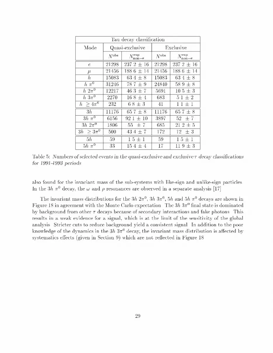
observed events in each class of the data sample is given in Table 5 for the two classi�cations.
Figure 16 shows the invariant mass for the quasi-exclusive selected h �0, h 2�0 decays.6 For
the h 2�0 invariant mass distribution a good agreement between the simulation and data is
observed, despite a slight discrepancy in the invariant mass distributions of the sub-systems
h �0 and �0�0 discussed in Section 9.2.
The invariant mass distributions for the h 3�0, h 4�0, 3h and 3h �0 decays are shown in
Figure 17 in good agreement with the simulation. For the 3h decays, a slight disagreement is
6For all the invariant mass plots the pion mass is assumed for the charged hadrons unless otherwise stated.
28
Tau decay classi�cation
Mode Quasi-exclusive Exclusive
Nobs Nexpnon�� Nobs N
expnon��
e 21298 237.2 � 16 21298 237.2 � 16
� 21456 188.6 � 14 21456 188.6 � 14
h 15083 63.4 � 8 15083 63.4 � 8
h �0 31246 78.7 � 9 24840 58.9 � 8
h 2�0 12217 46.3 � 7 5691 10.5 � 3
h 3�0 2270 16.8 � 4 683 5.1 � 2
h � 4�0 232 6.8 � 3 41 1.1 � 1
3h 11176 65.7 � 8 11176 65.7 � 8
3h �0 6156 92.1 � 10 3897 52. � 7
3h 2�0 1806 55. � 7 685 21.2 � 5
3h � 3�0 500 43.4 � 7 172 12. � 3
5h 59 1.5 � 1 59 1.5 � 1
5h �0 33 15.4 � 4 17 11.9 � 3
Table 5: Numbers of selected events in the quasi-exclusive and exclusive � decay classi�cationsfor 1991-1993 periods.
also found for the invariant mass of the sub-systems with like-sign and unlike-sign particles.
In the 3h �0 decay, the ! and � resonances are observed in a separate analysis [17].
The invariant mass distributions for the 3h 2�0, 3h 3�0, 5h and 5h �0 decays are shown in
Figure 18 in agreement with the Monte Carlo expectation. The 3h 3�0 �nal state is dominated
by background from other � decays because of secondary interactions and fake photons. This
results in a weak evidence for a signal, which is at the limit of the sensitivity of the global
analysis. Stricter cuts to reduce background yield a consistent signal. In addition to the poor
knowledge of the dynamics in the 3h 3�0 decay, the invariant mass distribution is a�ected by
systematics e�ects (given in Section 9) which are not re ected in Figure 18.
29

ALEPH ALEPH
h π0 h 2 π0
Eve
nts
/ 20
Mev
/c2
Eve
nts
/ 20
Mev
/c2
Figure 16: Invariant mass distributions for the h �0 and h 2�0 quasi-exclusive selected samples.The points with error bars show the observed distributions, the solid histograms representthe simulated distributions and the shaded histograms account for the expected � background
from the Monte Carlo computed with the measured branching ratios.
30

ALEPH ALEPH
ALEPH ALEPH
h 4 π0h 3 π0
3 h π03 h
Eve
nts
/ 50
Mev
/c2E
vent
s / 5
0 M
ev/c2
Eve
nts
/ 50
Mev
/c2E
vent
s / 7
5 M
ev/c2
Figure 17: Invariant mass distributions for the h 3�0, h � 4�0, 3h and 3h �0 quasi-exclusiveselected samples. The points with error bars show the observed distributions, the solidhistograms represent the simulated distributions and the shaded histograms account for the
expected � background from the Monte Carlo computed with the measured branching ratios.
31

3 h 3 π03 h 2 π0
5 h π05 h
ALEPHALEPH
ALEPHALEPH
Eve
nts
/ 100
Mev
/c2E
vent
s / 1
00 M
ev/c2
Eve
nts
/ 100
Mev
/c2E
vent
s / 1
00 M
ev/c2
Figure 18: Invariant mass distributions for the 3h 2�0, 3h 3�0, 5h and 5h �0 quasi-exclusiveselected samples. The points with error bars show the observed distributions, the solidhistograms represent the simulated distributions and the shaded histograms account for the
expected � background from the Monte Carlo computed with the measured branching ratios.
32

8 Extraction of branching ratios
In order to extract a measurement of the � branching ratios from this global analysis, the
number of observed events in a given class j after the non-� background subtraction divided
by the sum of all observed events de�nes the observed fraction of events fj in the class j. The
fraction fj is related to the branching ratios Bi to be determined by the following equation:
fj =
Pi Eij BiPik Eik Bi
; (4)
where Eij is the e�ciency matrix (de�ned in the previous section). The linear system de�ned
by the fj's is solved with the additional constraint
Xi
Bi = 1 : (5)
For convenience, a maximum likelihood technique is used to solve the system and to estimate
the errors.
It should be noticed that the e�ciency matrix Eij is independent of the � branching ratiosused in the Monte Carlo simulation, except for the subclasses contributing to each de�ned
class as shown in Table 3. The e�ect depends however on small branching ratios and the
procedure used in this correction relies on measured values. In this analysis the branching
ratios used for the Cabibbo-suppressed and Cabibbo-allowed decays are consistent with the
ALEPH measurements [5, 6].
A correction to the Eij e�ciency matrix is applied to take into account the de�cit of
16 % of fake photons in the simulation. This correction is computed as the opposite of the
e�ect obtained in the e�ciency matrix when the number of fake photons in the Monte Carlo
is reduced by 16 %. This linear procedure is justi�ed from studies made with the Monte
Carlo. As a check, a model producing this excess of fake photons was implemented in the
simulation and the complete �0 reconstruction procedure was repeated. The two methods
yield consistent results.
The analysis relies on the standard � decay description [10]. One could imagine unknown
decay modes not included in the simulation but since large e�ciencies are achieved in the �
selection it is di�cult to overlook them in the analysis. A notable exception could be low
momentum particles coming from decays like � ! eN0 with mN0 � m� and N0 not decaying
in the detector volume, so it is important to make sure that such decays are not present.
An independent measurement of the branching ratio for undetected modes by a direct search
was done in ALEPH [18], limiting this branching ratio to less than 0.11 % at 95 % CL and
justifying the assumption that the sum of the branching ratios for visible � decays is equal to
one.
33

9 Systematic uncertainties
The possible sources of systematic uncertainties come mainly from the particle identi�cation,
the selection of � pair events, and the photon and �0 reconstruction. The systematics
on the particle identi�cation and � event selection are described in detail in reference [4].
For the � hadronic decay modes reported in this paper special emphasis is given to the
systematics a�ecting the �0 reconstruction. In most cases, possible deviations in the Monte
Carlo simulation compared to the data are propagated to the e�ciency matrix and a new set
of branching ratios is derived. The di�erences with the reference values or the statistical error
of the test are quoted as systematic errors. With this procedure, the correlations among the
several classes are also taken into account.
9.1 Photon and �0 reconstruction
The relevant sources of systematic e�ects in the photon and �0 reconstruction are described
in the following. First, the systematics associated with the photon clustering algorithm are
examined.
� The ine�ciency of the clustering algorithm described in Section 5.2 is directly studied
with an independent sample of electrons from � decays. In this study the cut of the
distance between the electromagnetic cluster and the charged track is removed, so
electron showers are considered as photon candidates. Because of the magnetic bending
this method only covers the domain above 1 GeV. This study shows that the e�ciency
is well described by the simulation with a ratio of data over Monte Carlo essentially
energy independent, di�ering from unity by (0.23 � 0.15) %. The column with the Eclustlabel shows the derived systematics in Table 6.
� In the same table the systematic e�ect from a global energy scale (labeled as Escale) is
given. The uncertainty in the global energy scale error for the ECAL pad calibration
is taken to be 0:3% � 3%/pE (with E in GeV) from imperfect pad clustering
corrections [19].
� The spectrum of low energy photons belonging to resolved �0's is given in Figure 19
after subtraction of the fake photon contribution a�ecting this sample. The systematics
related to the fake photons are discussed below. The photon e�ciency is fairly well
reproduced by the simulation, in particular in the region below 1 GeV which was not
tested with electrons using the previous method. From the comparison in this region
the ine�ciency for photons in the data is larger by (4.4 � 3.4) % with respect to the
Monte Carlo. This correction is applied in the analysis. Changing the relative e�ciency
between data and Monte Carlo by 3.4 % yields the systematic uncertainties shown in
34

ALEPH
Pho
tons
/ 25
MeV
Figure 19: The points with error bars show the energy spectra below 2 GeV for the
reconstructed photons entering resolved �0's and the solid histogram from simulation, aftersubtraction of fake photons.
Table 6 in the column labeled as Elow. This error is equivalent to a shift of 20 MeV in
the e�ective threshold for �0 reconstruction.
� The minimal distance between the barycentre of an electromagnetic cluster and the
closest charged track in the same hemisphere is an important parameter to veto fake
photon candidates from the hadron interactions in ECAL at the expense of some
ine�ciency for the signal (� 3 % of the photons). The simulation of the e�ciency
for reconstructing genuine photons in the close environment of a charged hadron relies
on the description of hadronic and electromagnetic showers in the Monte Carlo. If the
photon shower is not identi�ed as a separate cluster, it is expected that the barycentre
of the compound shower will be shifted from the track impact point and the cluster will
be registered as a photon candidate if the distance exceeds the 2 cm cut value. The
distribution of this distance as given in Figure 20 for all photons reconstructed as genuine
shows a step rise above the minimum value in agreement with the simulation (the fact
that a few photons appear with a value below the cut is explained in Section 5.2). The
raw distribution for photons at the Monte Carlo generator level is given for comparison,
35

ALEPH
DATAMC
(cm)
Pho
tons
/ 0.
2 cm
Figure 20: The distribution of the distance between the barycentre of a reconstructed photonfrom a �0 and the closest charged track is given as points with error bars. The solid histogram
shows the Monte Carlo simulation and the dotted histogram corresponds to the distributionat the generator level. Both Monte Carlo histograms are normalized for distances larger than10 cm.
showing the ine�ciency associated to the hadronic environment in the electromagnetic
calorimeter. The e�ciencies can be directly compared for distances less than 8 cm and
the systematic uncertainty is derived from the statistical error of the comparison. The
possible disagreement between data and Monte Carlo can be e�ectively described by a
change in the cut value by less than 1 mm. The corresponding systematic uncertainties
appear in Table 6 labeled as d t.
� The variables that de�ne a pair of charged tracks coming from a conversion, such as the
invariant mass and the distance in the plane transverse to the beam between the two
tracks at the point of closest approach, show a good agreement between data and Monte
Carlo. The e�ect of the misidenti�cation probabilities in the particle identi�cation
quoted in Section 4 is found to be negligible. The di�erence in the fraction of converted
photons mentioned in Section 5.1 (which could produce a bias through the di�erence of
e�ciencies for converted and non-converted photons) also induces a negligible systematic
uncertainty.
Next, the systematics of the photon likelihood identi�cation are described.
36

Mode Elow d t Eclust Escale ref D�0 m�0 fake �Total�0
h 0.027 0.034 0.032 0.026 0.033 0.010 0.006 0.060 0.097
h �0 0.035 0.010 0.006 0.042 0.048 0.010 0.023 0.040 0.088
h 2�0 0.022 0.026 0.020 0.023 0.032 0.010 0.025 0.050 0.082
h 3�0 0.043 0.019 0.011 0.065 0.049 0.011 0.008 0.040 0.104
h � 4�0 0.041 0.020 0.010 0.065 0.013 0.011 0.008 0.020 0.085
3h 0.032 0.033 0.007 0.030 0.016 0.004 - 0.048 0.075
3h �0 0.032 0.013 0.002 0.025 0.010 0.004 0.002 0.025 0.051
3h 2�0 0.016 0.011 0.003 0.032 0.023 0.008 0.005 0.050 0.067
3h � 3�0 0.015 0.010 0.008 0.026 0.004 0.005 0.006 0.019 0.040
5h 0.008 0.001 - 0.002 0.004 0.002 - 0.001 0.010
5h �0 0.007 0.001 - 0.001 0.004 0.002 - 0.002 0.008
Table 6: Systematic e�ects a�ecting the �0 reconstruction in the quasi-exclusive classi�cation.
All these values are absolute (branching ratios in %). Symbols are de�ned in the text.
� To check the likelihood method, which uses di�erent estimators to tag the genuine
and fake photons, a careful study of the reference distributions of the probability
densities is needed. The simulation of hadronic interactions in the electromagnetic
calorimeter is studied in a selected sample of pions in data and in Monte Carlo. A
resonable description of the hadronic showers in the simulation is found, although slight
discrepancies concerning the modeling of uctuations of hadronic showers are observed
as seen in Figure 5. The simulation of fake photons from electromagnetic showers
presents as well some di�erences as shown in the d distribution in Figure 5. Di�erent
correction functions are evaluated with data and their uncertainties are propagated
to the corresponding estimators as stated in Section 5.3 taking the correlations into
account. The maximal e�ect observed in the branching ratios is given in Table 6 under
the column label ref by switching on and o� such corrections.
� An excess of fake photons is observed in data with respect to the Monte Carlo. This
excess is measured to be 16% in the data by comparing the relative weight of the
Monte Carlo distributions for genuine and fake photons to the data distributions. This
excess is corrected in the extraction of the branching ratios as described in Section 8.
The correction corresponds to an average excess of fake photons, but does not take into
account the relative contribution of electromagnetic and hadronic fake photons expected
to vary from channel to channel. Thus, a systematic uncertainty is assigned to each
channel by comparing the distributions of the P Res estimator of the rejected photons
for data and Monte Carlo. The relative number of rejected fake photons and the shape
37

of the respective distributions provide an estimate of the loss of events in this channel
due to unrecognized fake photons. This procedure yields systematic uncertainties which
are about half the full correction applied. The results are quoted in the column labeled
as fake in Table 6.
Finally, the systematics associated with the �0 procedure are discussed.
� In order to study the systematic e�ects a�ecting the �0 reconstruction, di�erent parame-
trizations are used for the resolutions and the e�ective mass needed in the computation
of P�0 for �0's with and without converted photons. The derived systematic uncertainty
is shown under label m�0 .
� The estimator for a pair of photons to originate from a �0, D�0
i;j , seems to indicate an
excess of data in the �rst bins (Figure 8). This indication can be interpreted as scale
factor between data and Monte Carlo distributions, corresponding to a shift around the
cut value which is found to be 0.00017 � 0.00009 by a �2 minimization. The derived
systematic e�ect when applying the shift measured in the data is given in Table 6 under
the column label D�0 .
Finally, in the last column in Table 6 the total error �total�0 from the �0 reconstruction is
computed as the quadratic sum of all components.
9.2 Tau selection and particle identi�cation
As explained in Section 3, the overall � pair selection e�ciency at the Z0 peak is measured
on � data directly and is found to be (78.84 � 0.13) %. The corresponding value for the
Monte Carlo is (78.99 � 0.09) %, which is in agreement with the previous value. Because
of the known discrepancies between Monte Carlo and data concerning the simulation of fake
showers in the electromagnetic and hadronic calorimeters, it is important to test that the �
pair selection does not contain a channel-dependent e�ciency not reproduced by the Monte
Carlo simulation. Such a hypothetical dependence would induce, in principle, a bias in the
e�ciency matrix. With a version of the � selection designed to be more sensitive to such fake
showers by removing the energy thresholds for neutral objects, the global branching ratio
analysis is repeated so that a systematic uncertainty is quoted for every channel. Table 7
shows the derived value in the column � - sel.
As 16 % of the data sample in this analysis corresponds to o�-peak energies, the Monte
Carlo simulation is used to determine the drop of � selection e�ciencies, which is found to
be 1.7 % and 0.8% at + and �2 GeV of the peak energy, respectively. This is due to initial
state radiation and no channel-dependent e�ect is observed.
38

DATA
DATA
MC
MC
a)
b)
ALEPH
ALEPH
Hem
isph
eres
Hem
isph
eres
Figure 21: Distribution of charged tracks in the opposite hemispheres in which �ve chargedhadrons are selected (�gure a) and �ve hadrons at least (any combination of charged andneutral hadrons, �gure b).
The uncertainties on the contribution of non-� background are now considered. In spite
of the non-� background being less than one percent over the whole sample, its distribution
is not uniform in the di�erent reconstructed classes. In particular, the qq background should
a�ect primarily the classes of high hadron multiplicity. In Figure 21 the distribution of charged
tracks in the opposite hemispheres in which �ve hadrons are selected is shown with the Monte
Carlo expectations and a good agreement is observed. A maximal variation of � 50 % for
this background in each channel leads to a small contribution which is included in the �nal
systematic error.
Of particular interest is the electron and muon contamination in the one-prong hadron
sample, which is known from other studies not to be completely reproduced by the Monte
Carlo. However, a procedure is developed using data to actually measure the relevant
e�ciencies in each data sample [4]. The quoted systematics for such e�ects are given in
the column labeled as p - id of Table 7.
39

9.3 Tracking and secondary interactions
The tracking uncertainties contribute di�erently according to the topology. For the one-
prong hemispheres, they do not enter signi�cantly since no absolute e�ciency is needed in
the global analysis. In the three-prong decays, their e�ect is strongly reduced since 2, 3,
and 4 charged tracks are accepted in the three-prong de�nition. Possible uncertainties in the
track reconstruction coming either from the sharing of coordinate points in the multi-track
environment or from the description of K0S ! ���+ decays are also investigated since the
feed-across between one- and three-prongs could be a�ected. In a speci�c analysis dealing with
the K0S reconstruction, no signi�cant discrepancy with respect to the simulation is observed.
Analyzing � pair events in which the two hemispheres have like-sign charges in Monte Carlo
and in data allows to test the probability to lose the two like-sign particles in a three-prong
hemisphere. According to the Monte Carlo about half of the sample of like-sign hemispheres
originates from three-prong decays if a strong cut on the track association to the interaction
point (d0) is applied; a total of 291 � 17 events are observed in data in agreement with
269 � 12 expected by the Monte Carlo simulation. The proportion of two charged tracks in
the three-prong hemispheres is also observed to be higher in the data by (7.6 � 4.5)%. These
measurements are interpreted in terms of tracking ine�ciency and are used to compute the
quoted systematic errors given in the column labeled tracking.
Secondary interactions of hadrons in the detector can a�ect the reconstructed topology of
�nal states for both charged particles and �0's. The e�ect on charged particles depends on
their momenta and the radial distance at which the interactions takes place because of the
d0 cut used to de�ne a good track. It is important to test the simulation of interactions in
the Monte Carlo and assess the consequences on the feedthrough of events between di�erent
� decays classes.
The basic ingredient used for this analysis is the d0 distribution of charged tracks for each
topology. Here d0 is given a sign from the track angular momentum at the point of closest
approach to the beam crossing point in the plane transverse to the beam direction. In this
way, the sign of d0 is equal to the charge of a secondary track collinear to the interacting
hadron at the production point. Figure 22 shows such distributions for one and three-prong
decays. Primary tracks from the beam-beam interaction point present a sharp d0 peak with a
fall-o� which is underestimated by the simulation. This has no consequence for this analysis
which uses a wide d0 cut at 2 cm. Beyond this peak, long tails are observed which are well
explained by the simulation as originating from secondary interactions and tracking problems
in a multi-track environment (even in one-prong hemispheres about 20 % of the decays have
at least one additional track from photon conversions). Note the expected excess of positive
secondary tracks reproduced by the simulation. The agreement between data and Monte Carlo
can be expressed as the ratio of events for jd0j larger than 0.5 cm which is 1.004 � 0.045
and 0.983 � 0.031 for one and three-prong decays, respectively. The average interaction
probability for a track in the sample is 2.3 % from the simulation, mostly at small d0 values not
a�ecting signi�cantly the topology. Agreement is observed for the tails of the d0 distributions
40

ALEPH
One-prong
Three-prong
Eve
nts
/ 0.1
cm
Eve
nts
/ 0.1
cm
(cm)
Figure 22: d0 distribution for one and three-prong hemispheres. The points with error barsshow the data and the solid histogram the Monte Carlo. The shaded histograms correspondto the secondary interactions from the simulation. For the three-prong decays only the largestd0 value is plotted.
in data and Monte Carlo for all hadron topologies, checking the simulation of charged tracks
and �0's in secondary interactions. From this comparison, systematic uncertainties on the
branching ratios are quoted in Table 7 under the heading inter.
9.4 Tau decay dynamics
Uncertainties in the dynamics of the hadronic � decays can lead to systematics e�ects when
computing the e�ciency matrix. Studying the e�ciencies as a function of hadronic mass
checks for possible bias depending on the resonance structure in the hadronic �nal state.
These checks are performed for all the � decay categories. In the h �0 �nal state a good
description of the � - �0 interference is found, and no dependence on the h �0 invariant mass
is observed for the e�ciency. Alternative models for the description of the dynamics of the
41

a1 resonance have been proposed in reference [20]. The associated systematic e�ect due to
the uncertainty on the ratio of D to S waves [21, 22] is computed through a reweighting of
the Monte Carlo matrix elements. Also, � decays in the 3h 2�0 �nal state were generated
with a non-resonant amplitude. The new version of the generator [23] now includes the
resonant channel ��0! which dominates this class, as reported by CLEO [12]. Dedicated
Monte Carlo productions allow to correct these e�ciencies for the involved channels. The
estimated systematic uncertainties are quoted in the column labeled "Dyn.
The e�ciency matrices for right-handed and left-handed � 's are computed separately from
the simulation. Using the � polarization measured by ALEPH [19] within the experimental
uncertainty, the resulting e�ciencies are evaluated. The e�ect on the branching ratios is
found to be small, and it is included in the �nal systematic errors.
9.5 Summary on systematic uncertainties
Mode �total�0 ���sel p-id tracking inter "Dyn MCstat �total
sys
h 0.097 0.029 0.019 - 0.014 - 0.036 0.110
h �0 0.088 0.014 0.017 - 0.022 - 0.051 0.106
h 2�0 0.082 0.017 0.003 - 0.010 0.040 0.045 0.104
h 3�0 0.104 0.019 - - 0.015 0.008 0.033 0.112
h � 4�0 0.085 0.006 - - 0.011 - 0.017 0.088
3h 0.075 0.014 - 0.020 0.026 0.006 0.028 0.088
3h �0 0.051 0.034 - 0.009 0.021 0.007 0.031 0.073
3h 2�0 0.067 0.011 - 0.001 0.009 0.012 0.025 0.074
3h � 3�0 0.040 0.013 - - 0.007 0.010 0.016 0.047
5h 0.010 0.004 - 0.004 0.005 - 0.004 0.013
5h �0 0.008 0.003 - 0.001 0.002 - 0.003 0.012
Table 7: Summary of systematics errors for the branching ratios obtained from the quasi-exclusive classi�cation. Dashes denote negligible contributions. All these values are absolute
(branching ratios in %). Symbols are de�ned in the text.
In the last column of Table 7 the total systematic uncertainty (�totalsys ) is given for every
class, including the contribution due to Monte Carlo statistics which is shown in the same
table with label MCstat.
A consistency test regarding the classi�ed hemispheres is done by looking at the correlation
in the classi�cation of the opposite hemispheres of a given � pair event. A new matrix of
14 � 14 classes is created from the Monte Carlo simulation after weighting every cell by the �
branching ratios measured from this analysis and taking into account the non-� background.
42

Mode 0 e � h h �0 h 2�0 h 3�0 h � 4�0 3h 3h �0 3h 2�0 3h 3�0 5h 5h �0
0 1.2 2.3 1.6 0.6 1.2 0.9 0.1 2.6 0.4 0.1 1.3 1.5 0.4 0.6
e 1.1 1.3 0.8 2.0 1.1 0.1 0.6 0.3 0.3 0.3 2.2 1.8 0.9
� 1.5 0.4 1.7 1.9 1.3 0.7 2.4 0.4 0.4 1.0 0.1 1.1
h 1.4 1.1 1.4 0.3 0.2 1.4 1.0 0.7 1.1 0.1 0.1
h �0 2.1 0.7 1.0 2.5 1.1 0.2 1.7 0.7 0.6 1.5
h 2�0 1.0 1.7 0.9 0.9 1.1 0.5 0.4 0.8 1.8
h 3�0 1.1 0.1 0.4 0.1 0.1 2.0 0.6 1.
h � 4�0 - 0.2 0.6 0.5 1. - -
3h 0.8 0.2 0.6 1.7 1.0 1.8
3h �0 0.1 1.0 0.6 1.1 0.6
3h 2�0 2. 0.4 0.5 -
3h � 3�0 0.6 - -
Table 8: Di�erence between the number of observed � pair events in data and that expectedfrom simulation, divided by the statistical error. Bold numbers imply a minus sign. The label\0" stands for the small fraction of � decays which are not classi�ed, essentially �nal stateswith one charged particle (not an electron) with P< 2 GeV/c and no reconstructed �0.
The di�erence between the number of measured � pair events (one hemisphere classi�ed as
class i and the opposite as j) on data and that expected from simulation with the measured
branching ratios divided by its statistical error is shown in Table 8 for every cell. The overall
�2 of 91.2 for 96 degrees of freedom is satisfactory.
Some of the � hemispheres are not classi�ed because they contain one charged particle
with a momentum smaller than 2 GeV and no reconstructed �0 (class 0 in Table 8). The
fraction of events with these hemispheres is consistently reproduced by the simulation with a
�2 of 14.8 for 14 degrees of freedom.
10 Quasi-exclusive and exclusive results
In this section the results of the global branching ratio analysis are given for the quasi-exclusive
and the exclusive classi�cations. Table 9 shows the results of the quasi-exclusive branching
ratio measurements with their statistical errors, and the total estimated systematic error as
described in the previous section. These results only refer to given topologies, which are not
yet corrected for at this stage for additional kaons. As these results are obtained with a
constraint and because of signi�cant mixing between classes with several �0's, the values are
43

correlated. In Table 10 the correlation coe�cients of the covariance matrix are given for the
measured branching ratios.
Mode
(before kaon
subtraction)
Value (%) �stat �sys �total
B(� ! h �� ) 12.44 0.11 0.11 0.16
B(� ! h �0 �� ) 25.98 0.15 0.11 0.19
B(� ! h 2�0 �� ) 9.68 0.13 0.10 0.17
B(� ! h 3�0 �� ) 1.34 0.09 0.11 0.14
B(� ! h � 4�0 �� ) 0.17 0.04 0.09 0.10
B(� ! 3h �� ) 10.02 0.10 0.09 0.13
B(� ! 3h �0 �� ) 4.45 0.09 0.07 0.12
B(� ! 3h 2�0 �� ) 0.54 0.07 0.07 0.10
B(� ! 3h � 3�0 ��) 0.11 0.04 0.05 0.06
B(� ! 5h ��) 0.080 0.011 0.013 0.017
B(� ! 5h �0 �� ) 0.018 0.007 0.012 0.014
Table 9: Quasi-exclusive hadronic branching ratios before any subtraction for the kaon modes.The �rst error is statistical, the second systematic, and the last one gives the total uncertainty.
Mode � h h �0 h 2�0 h 3�0 h � 4�0 3h 3h �0 3h 2�0 3h 3 � �0 5h 5h �0
e -0.190 -0.151 -0.261 -0.094 -0.029 -0.006 -0.121 -0.073 -0.009 -0.009 -0.006 -0.001
� 1.000 -0.148 -0.246 -0.086 -0.029 -0.005 -0.116 -0.069 -0.009 -0.009 -0.006 -0.001
h 1.000 -0.315 -0.048 -0.024 -0.004 -0.102 -0.051 -0.007 -0.008 -0.003 0.000
h �0 1.000 -0.413 0.011 -0.007 -0.160 -0.115 -0.012 -0.016 -0.009 -0.001
h 2�0 1.000 -0.374 0.043 -0.054 -0.045 -0.016 -0.011 -0.001 0.001
h 3�0 1.000 -0.373 -0.018 -0.014 0.004 -0.015 0.003 0.010
h � 4�0 1.000 -0.002 -0.007 -0.012 -0.022 0.008 -0.003
3h 1.000 -0.235 0.001 -0.004 -0.032 +0.001
3h �0 1.000 -0.207 -0.065 -0.006 -0.012
3h 2�0 1.000 -0.281 0.008 0.008
3h � 3�0 1.000 0.006 0.
5h 1.000 -0.111
Table 10: Correlation coe�cients for the quasi-exclusive analysis.
44

An independent global check of the understanding of the �0 reconstruction is performed
by repeating the complete analysis with the exclusive classi�cation. In this way the single
photons are not counted as �0's anymore. Instead of rejecting these events a new class is
designed for the topologies � 1h + � 0�0+ � 1 , the so-called single photon class. This new
class is expected to be populated essentially by \background" from standard decays where at
least one photon has been lost. However, a small signal is expected in this last class from the
following channels with non-�0 photons in the �nal state:
� B(� ! �! ��) � 0:17% with ! ! �0 [17].
� B(� ! ��0� ��) � 0:08% with � ! ; �+�� [13].
� B(� ! ��0! �� ) � 0:04% with ! ! �0 [12].
Mode e � h h �0 h 2�0 h 3�0 h 4�0 3h 3h �0 3h 2�0 3h 3�0 5h 5h �0
h �0 0.16 0.07 1.24 54.50 9.67 1.87 0.81 0.30 0.80 0.18 0.10 0. 0.
�0.01 �0.01 �0.04 �0.11 �0.11 �0.13 �0.41 �0.02 �0.05 �0.06 �0.10
h 2�0 0. 0. 0.10 1.04 30.97 14.74 4.88 0.03 0.21 0.75 0.38 0. 0.24�0.01 �0.02 �0.17 �0.33 �1.09 �0.01 �0.02 �0.12 �0.19 �0.23
h 3�0 0. 0. 0.01 0.06 1.00 17.20 32.43 0. 0.04 0.16 0.48 0. 0.�0.01 �0.01 �0.04 �0.36 �2.12 �0.01 �0.06 �0.21
h � 4�0 0. 0. 0. 0. 0.03 0.28 4.48 0. 0. 0. 0.19 0. 0.
�0.01 �0.05 �0.92 �0.14
3h �0 0. 0. 0.13 0.29 0.17 0.06 0. 2.75 43.44 9.81 3.25 3.44 9.92
�0.01 �0.01 �0.01 �0.02 �0.06 �0.26 �0.46 �0.55 �0.76 �1.44
3h 2�0 0. 0. 0.04 0.08 0.29 0.28 0.38 0.31 2.78 24.53 18.62 0.19 3.22�0.01 �0.01 �0.02 �0.05 �0.28 �0.02 �0.09 �0.59 �1.22 �0.19 �0.85
3h � 3�0 0. 0. 0.02 0.04 0.11 0.39 1.00 0.06 0.25 2.54 15.20 0. 0.47
�0.01 �0.01 �0.01 �0.06 �0.45 �0.01 �0.03 �0.21 �1.11 �0.33
5h �0 0. 0. 0. 0. 0. 0. 0. 0.01 0.01 0. 0. 0.95 24.74
�0.01 �0.01 �0.43 �2.14
Table 11: E�ciency matrix for the exclusive classi�cation of hadronic decays. The e�ciencies
are expressed in percent with their statistical error only. The generated classes are given in
the �rst row, and the reconstructed classes in the �rst column.
In order to illustrate the exclusive classi�cation, the e�ciency matrix is shown in Table 11
for the classes containing at least one �0 (otherwise there is no change with respect to the
previous quasi-exclusive classi�cation) . As the exclusive classi�cation is more rigorous with
the �0 identi�cation, less mixing is obtained in the classes with several �0's. The invariant
mass distributions for the h 3�0, h � 4�0, 3h 2�0 and 3h � 3�0 are plotted in Figure 23. An
enhancement of the signal over the background is observed with respect to the quasi-exclusive
classi�cation.
Table 12 shows the results of the exclusive analysis. For the classes with no �0 the
results are essentially unchanged from the quasi-exclusive analysis. On the other hand, for
45

h 4 π0h 3 π0
3 h 3 π03 h 2 π0
ALEPHALEPH
ALEPHALEPH
Eve
nts
/ 110
Mev
/c2E
vent
s / 1
10 M
ev/c2
Eve
nts
/ 140
Mev
/c2E
vent
s / 1
40 M
ev/c2
Figure 23: Invariant mass distributions for the h 3�0, h � 4�0, 3h 2�0 and 3h 3�0 exclusiveselected samples. The points with error bars show the observed distributions, the solidhistograms represent the simulated distributions and the shaded histograms account for the
expected background from other � decays with the measured branching ratios.
46

Mode Value (%) �stat �sys �Bexpected �B ��B
B(� ! h ��) 12.44 0.11 0.10 - - -
B(� ! h �0 �� ) 25.76 0.17 0.16 - 0.22 0.16
B(� ! h 2�0 ��) 9.52 0.20 0.25 0.17 0.16 0.25
B(� ! h 3�0 ��) 0.85 0.22 0.21 0.10 0.50 0.20
B(� ! h � 4�0 �� ) 0.37 0.10 0.12 - -0.21 0.11
B(� ! 3h �� ) 10.02 0.10 0.07 - - -
B(� ! 3h �0 ��) 4.41 0.09 0.08 - 0.04 0.08
B(� ! 3h 2�0 �� ) 0.49 0.08 0.10 0.01 0.05 0.10
B(� ! 3h 3�0 �� ) 0.20 0.06 0.06 - -0.10 0.06
B(� ! 5h �� ) 0.080 0.011 0.009 - - -
B(� ! 5h �0 ��) 0.008 0.006 0.009 - 0.010 0.007
B(� ! � 1h � 0�0 � 1 �� ) 0.67 0.22 0.47 0.28 - -
Table 12: Exclusive hadronic branching ratios and di�erences with respect to the quasi-exclusive measurements.
the modes with �0's, the di�erences �B (quasi-exclusive branching ratio minus exclusive
branching ratio) are given in Table 12. The statistical error (�stat) and the systematic error
(�sys) of the exclusive branching ratios are also speci�ed. In order to evaluate the systematic
error in the measurement of the exclusive branching ratios the procedure described in Section 9
is repeated with the exclusive classi�cation. The largest di�erences appear in the systematic
uncertainties a�ecting the �0 reconstruction as one would expect, since any uncertainty which
causes the loss of a photon implies, consequently, the loss of its associated �0. This is not the
case in the quasi-exclusive classi�cation. The systematic uncertainties associated with the
exclusive branching ratios, shown in Table 12, are therefore substantially larger than those
given in Table 9.
The errors ��B on �B given in Table 12 include the error due to the statistical uctuation
of events not in common and to uncorrelated systematics. The changes in all classes are
consistent within the errors and with the expected \hadronic" signal (mainly, in the h 2�0
and h 3�0 channels ) from decays with photons not coming from �0's. However, the overall
agreement is only fair with a �2 of 14.4 for 8 degrees of freedom. Although no clear pattern
emerges in Table 12 to explain this fact, it should be reminded that the exclusive branching
ratio analysis is more sensitive to systematic uncertainties in the �0 reconstruction.
47

For the � 1h + � 0�0+ � 1 class (dominated by background from other classes, which
is properly subtracted out by the method) a signal of (0:67 � 0:22 � 0:47)% is observed,
where the �rst error is statistical and the second systematic. After subtraction of the expected
signal, a limit is derived for a new non-�0 photonic channel (excluding radiative photons which
have been eliminated earlier as discussed in Section 6.3), which is found to be:
Bnew(� ! � 1h+ non-�0 0s �� ) < 1:6 % at 95 % CL: (6)
In deriving (6), the systematic error has been conservatively scaled by a factor of 1.34 to take
into account the �2 of the channel to channel comparison given in Table 12 and quoted above.
In conclusion, from the comparison of the branching ratios obtained with the quasi-
exclusive and exclusive classi�cations, no inconsistency is found, and the description of the
hadronic modes is complete at the level of precision quoted. Therefore, since the quasi-
exclusive results are less a�ected by the systematic e�ects and are statistically more precise
these values are taken as the �nal results and they are discussed in the next sections.
11 Update on � decays to charged and neutral kaons
The study of charged and neutral kaon production in � decays given in reference [5, 6] was
mainly limited by the statistics of the data sample. The same approach is followed when
analyzing the 1993 data sample; the reader is referred to the previous publications [5, 6] for
more details. A summary of the selected numbers of events, e�ciencies and contaminations
in the di�erent � decays into kaons is given in Table 13. The charged kaon fraction in a given
sample is derived by �tting the observed ionization loss distribution to a linear combination
of the expected pion and kaon distributions. The di�erence between the dE=dx measurement
and the expectation value for a pion divided by the experimental resolution (x�) is shown in
Figure 24 for one-prong hadronic � decays for the whole data sample. The �tted distribution
is plotted, with the �, e and � individual contributions and the derived K component. The
ratio of the dE=dx probability density for kaons to the sum of the probability densities for
kaons and pions de�nes a kaon estimator PK . The distributions of PK are plotted in Figure 25
for the hK0L and h �0K0
L samples, where the charged kaon signal is evident and in agreement
with the simulation.
For completeness, the distributions of the relative excess of energy in the hadronic
calorimeter (�E) with respect to the charged particle momentumand the angular displacement
of the hadronic energy barycentre (��) with respect to the impact of the charged track are
shown in Figure 26 for the hK0L and h �0K0
L samples. Consistency is observed with the Monte
Carlo for both samples. The invariant mass distribution for the K� resonance is plotted in
Figure 27 for the �K0L sample. Finally, the updated branching ratios for these kaons modes
are reported in Table 14.
48

Mode Decays E�ciency (%) Background (%)
� ! K� � 0�0K0 �� 1610 � 55 63.8 � 0.7 -
� ! K� �� 728 � 37 55.6 � 1.0 14 � 4
� ! K� �0 �� 395 � 27 44.0 � 1.4 10 � 3
� ! K� 2�0 �� 59 � 11 30.3 � 1.8 37 � 13
� ! �� K0 �� 98 � 10 6.3 � 0.2 19 � 5
� ! K� K0 �� 13 � 4 3.0 � 0.2 8 � 8
� ! �� �0 K0 �� 23 � 5 2.9 � 0.4 35 � 9
� ! K� �0 K0 �� 5 � 2 2.9 � 0.8 20 � 20
Table 13: Summary of statistics, e�ciencies and backgrounds for the � decaymodes containing
kaons.
K
µ
π
e
ALEPH
Figure 24: Fitted x� distribution in one-prong hadronic � decays. The points with error
bars correspond to data, the solid lines show the �, e and � contributions and the �tted K
component.
49

h K0L
Kπ
ALEPH
h π0 K0L
Kπ
ALEPH
Figure 25: The distributions of the charged kaon dE/dx estimator for the hK0L and h �0K0
L
selected samples. The points with error bars show the observed distribution, and the solidhistogram the simulation. The shaded histograms show the expected � contribution.
Mode Value (%) �stat �sys �total
B(� ! K� � 0�0K0 �� ) 1.70 0.05 0.06 0.08
B(� ! K� �� ) 0.72 0.04 0.04 0.06
B(� ! K� �0 �� ) 0.52 0.04 0.05 0.06
B(� ! K� 2�0 ��) 0.08 0.02 0.02 0.03
B(� ! �� K0 �� ) 0.79 0.10 0.09 0.13
B(� ! K� K0 �� ) 0.26 0.09 0.02 0.09
B(� ! �� �0 K0 ��) 0.32 0.11 0.05 0.12
B(� ! K� �0 K0 �� ) 0.10 0.05 0.03 0.06
B(� ! K�� �� ) 1.39 0.09 0.10 0.13
Table 14: Branching ratios for modes with kaons. The statistical and systematic errors arealso shown.
50

πK0L
KK0L
ALEPH
πK0L
KK0L
ALEPH
ππ0K0L
Kπ0K0L
ALEPH
ππ0K0L
Kπ0K0L
ALEPH
Figure 26: In the upper plots the distributions of �E and �� are shown for the �K0L and KK0
L
samples. The points with error bars show the data for the whole hK0L sample, and the shaded
and hatched histograms correspond to the Monte Carlo simulation for the �K0L and KK0
L
samples. The lower plots follow the same speci�cations as above, but they correspond to the
��0K0L and K�0K0
L samples.
51

ALEPH
non-Kπ0
K*E
VE
NT
S/5
0 M
eV/c2
(GeV/c2)
ALEPH
non-K0π
K*
EV
EN
TS
/125
MeV
/c2
(GeV/c2)
Figure 27: Invariant mass distributions for theK�0 (left) and �K0L (right) systems. The points
with error bars show the measured invariant mass distribution, and the shaded histogramsstand for the simulation. The hatched histograms correspond to the background in the K�0
and �K0L decays.
12 Corrected branching ratio results
The results of the quasi-exclusive classi�cation after subtraction of kaon modes and !, � decays
into non-�0 photons are given in Table 15. When subtracting such modes, their e�ciencies
are taken into account and the �nal error includes the statistical and systematic components
of this correction. These results are consistent with the published ALEPH values with 1989
and 1990 data [3].
The values used to perform such subtractions are described in the following:
� For the � decay modes into K�, K�K0, K��, K�2�0, ���0K0 and K��0K0, the
measured values given in Table 14 are taken.
� For the � decay mode into �!, the omega fraction, f! = (38:3 � 2:9) % [17], is also
used together with the 3h �0 decay rate measured in the global analysis.
� For the � decay mode into ��0!, 80 % of the branching ratio for 3h 2�0 is used since
this channel is observed to be dominated by the ! resonance [12].
� For the � branching ratio into �K0K0 the value 0.3 % is taken with � 50 % uncertainty
and the assumption that the �nal states �K0LK
0L, �K
0SK
0S and �K0
SK0L are in the ratios
1:1:2.
52

� No attempt is made to subtract the decay modes K��+�� and K�K+��, in the 3h
class at this time.
Mode Value (%) �stat �sys �total
B(� ! h �� ) 11.78 0.11 0.13 0.17
B(� ! � ��) 11.06 0.11 0.14 0.18
B(� ! h �0 ��) 25.76 0.15 0.13 0.20
B(� ! � �0 �� ) 25.30 0.15 0.13 0.20
B(� ! h 2�0 �� ) 9.29 0.13 0.11 0.17
B(� ! � 2�0 �� ) 9.21 0.13 0.11 0.17
B(� ! h 3�0 �� ) 1.17 0.09 0.11 0.14
B(� ! h � 4�0 �� ) 0.16 0.04 0.09 0.10
B(� ! 3h ��) 9.50 0.10 0.11 0.15
B(� ! 3h �0 �� ) 4.30 0.09 0.09 0.12
B(� ! 3h 2�0 �� ) 0.50 0.07 0.07 0.10
B(� ! 3h � 3�0 ��) 0.11 0.04 0.05 0.06
B(� ! 5h ��) 0.080 0.011 0.013 0.017
B(� ! 5h �0 �� ) 0.018 0.007 0.012 0.014
Table 15: Quasi-exclusive hadronic branching ratios after subtraction of the contributionsfrom charged and neutral kaons, and non-�0 photonic !, � decays.
Although the leptonic branching ratios are also obtained in the global analysis, they are
not discussed in this paper. They are in good agreement with the results of the dedicated
analysis described in reference [4]: from the quasi-exclusive classi�cation the corresponding
branching fractions for the � ! e�e�� and � ! ����� decays are (17.81 � 0.11) % and
(17.34 � 0.11) %, where only the statistical error is given. The corresponding values are
(17.79 � 0.12) % and (17.31 � 0.11) % for the dedicated leptonic analysis. The di�erences
are compatible within an expected uncertainty of 0.05 % from statistics and systematics not
in common.
13 Discussion of the results
In this section the results presented in this paper are analyzed, discussed and compared to
theoretical estimates.
53

� ! h ��
The � ! h �� branching ratio is shown in Figure 28 before any kaon subtraction and
compared to the existing measurements. After K0 removal, excellent agreement is found
between the decay rate of � ! h �� (11.78 � 0.17) % and the Standard Model predictions
equal to (11.75 � 0.06) % and (11.80 � 0.13) % according to references [24, 25], respectively,
where the ALEPH � lifetime measurement of (293.7 � 2.7 � 1.6) fs [26] is used. It is possible
to express this comparison for the � ! � �� decay as a test of �-� universality in the V�Acharged weak current. Using the measured � and � lifetimes and the branching ratio of the
decay �! ��, together with the radiative corrections relevant to both processes [24, 26, 27],
the obtained value isg�
g�= 1:0015 � 0:0098 :
A similar test is performed with � ! K �� and K ! �� decays, yielding
g�
g�= 0:997 � 0:042 :
Combining both results (1.0013 � 0.0095), the �-� universality hypothesis holds at the 1%
level in these channels.
Moreover, the ratio of the decay rates � ! K �� and � ! � ��
B(� ! K �� )
B(� ! � �� )= 0:0651 � 0:0055 ;
measures the ratio of the f� and fK decay constants according to the following equation:
f�
fK= tan �c
vuut B(� ! � �� )
B(� ! K �� )
m2
� �m2K
m2� �m2
�
!; (7)
once the kinematic factors and the Cabibbo angle �c are considered. The ratio of the � and
K decay constants is found to be:
f�
fK= 0:825 � 0:035 :
� ! h �0��
The most precise measurements for the � ! h �0 �� branching ratio are drawn in Figure 28
including the kaon contributions as stated in Table 3. Although the earlier measurements
favour a lower h �0 branching ratio, the newer measurements [28, 29, 30], and in particular
the present determination prefer a higher value. The hypothesis of the conserved vector
current (CVC) allows to derive a value for the ratio of � ! � �0 �� and � ! e �e ��
54

using e+e� data through an isospin rotation. Isospin invariance of the quark currents coupled
to gauge bosons is imbedded in the Standard Model which naturally incorporates the CVC
property. From the measured electron branching ratio of (17.79 � 0.12) % [4], the predicted
� ! � �0 �� branching ratio is (24.6 � 0.7) % [31], which is in good agreement with the
value of (25.30 � 0.20) % obtained from this analysis within the larger uncertainties arising
from the e+e� data.
Assuming vector meson dominance, the K� Cabibbo-suppressed decay can be compared
to the ��0 decay to extract the ratio of the � and K� decay constants according to
f�
fK�= tan �c
vuut B(� ! � �� )
B(� ! K� ��)
m2
� �m2K�
m2� �m2
�
!vuutm2� + 2m2
K�
m2� + 2m2
�
; (8)
which yieldsf�
fK�
= 0:931 � 0:044 :
The normalization of the decay constants in the vector current is chosen to have the same
units as in the pseudoscalar case. This ratio shows a similar magnitude with the above
f�=fK, and it is in fair agreement with the value of one which can be inferred from the naive
application of the Das-Mathur-Okubo (DMO) sum rule in the single-resonance and narrow
width assumptions [32, 33]. In other words, the measured ratio
B(� ! K� ��)
B(� ! � �� )= 0:0549 � 0:0052 :
is consistent with the DMO prediction of 0.0476 and is similar in magnitude to the ratio of
the � ! K �� and � ! � �� decay rates.
� ! h 2�0�� and � ! 3h ��
The available measurements for the � ! h 2�0 �� branching ratio are plotted in Figure 28,
after subtraction of the K0S component. The ALEPH measurement (9.29 � 0.17) % is
consistent with the PDG 94 (9.0 � 0.4) % [27] value.
Figure 29 shows the branching fractions for � ! 3h �� , with the K0S component
subtracted. Previously published measurements lead to a world average of (8.0 � 0.4) % [27]
with measurements spreading over a considerable range. New measurements of this decay
rate obtained from � 's produced in Z0 decays, presented here and in reference [34], are
inconsistent with this average. Possible sources of systematic discrepancies have already
been discussed [35].
The 3h and h 2�0 channels are observed to be dominated by the a1 ! �� resonance.
Therefore, isospin invariance predicts equal decay rates for 3� and � 2�0, ignoring small
phase-space corrections. Subtracting the contributions of the decays � ! K��+�� �� and
55

� ! K�K+�� �� [14, 15] from the measured 3h branching fraction, the value (8.94 � 0.20) %
is derived for the �� ! ���+�� �� decay. This value is in agreement with the � ! � 2�0 ��decay rate of (9.21 � 0.17) %. No direct theoretical estimate can be made for the � ! 3���decay rate. However, a consistency argument can be developed through the V�A structure
of the hadronic current: the axial and vector hadronic widths should be approximately equal.
Small non-perturbative QCD corrections are applied [36, 37] and the � and 5� decay widths
(given in this section) are taken into account to derive an estimate of (18.06 � 0.86) % for
the total 3� width (���+�� and ��2�0). This value compares well to the above result of
(18.15 � 0.26) %.
� ! h 3�0�� , � ! 3h �
0�� , � ! 5h �0
�� and � ! 3h 3�0��
For the h 3�0 decay mode, the ALEPH measurement shows good agreement with the
published CLEO result [38], as drawn in Figure 28. In addition, the CVC prediction for
the � ! � 3�0 �� decay, (1.07 � 0.05) % [31], is consistent with the ALEPH result of
(1.17 � 0.14) %.
Signi�cant progress is achieved in the three-prong � decays where exclusive decays
containing up to three �0's are reported in this paper. There are two CVC predictions for the
� ! 3� �0 �� decay, (4.2 � 0.3) % [31] and (4.8 � 0.7) % [36], which are in agreement with
the measured value (4.30 � 0.12) %.
The 5h �0 branching fraction is in agreement with the recently published CLEO
results [39], as plotted in Figure 29. From the CVC prediction for � ! 6� �� and isospin
symmetry, a lower limit for the � ! 5� �0�� decay equal to (0.027 � 0.005) % [31] is inferred,
which is close to the ALEPH measurement (0.018 � 0.014) %. For the decay � ! 3h 3�0 a
branching ratio value of (0.11 � 0.06) % is obtained. This value is larger than the estimates
from CVC or 5h �0 using isospin symmetry, which are in the range (0.02{0.08) %, but it is
consistent within the errors. In fact, the sum of the 5h �0 and the 3h 3�0 decays adds up to
(0.128 � 0.062) % in agreement with the CVC prediction of (0.13 � 0.02) % for the six pion
�nal state.
� ! h 4�0�� , � ! 3h 2�0
�� and � ! 5h ��
The � ! h 4�0�� , � ! 3h 2�0 �� and � ! 5h �� branching ratios show a agreement
with the CLEO measurements [12, 38, 39] as plotted in Figures 28 and 29. In fact, a higher
decay rate for � ! 3h 2�0�� , when compared to its isospin partner � ! 5h �� , is found.
From the measurements given in Table 15, the branching ratio for the �ve pion �nal state is
found to be (0.65 � 0.14) %, once the � ! ���0 �� contribution is subtracted out. This
result is in rough agreement with the � 1 % prediction using the partially conserved axial
current hypothesis [40].
Finally, Figure 30 shows exclusive � decay branching ratios involving kaons in the �nal
state. The ALEPH measurements are in agreement with the CLEO and L3 results [41, 42].
Avoiding the di�culty to select the isovector part from the isoscalar component in e+e� data,
56

several crude theoretical estimates exist for the � ! KK0 �� decay neglecting possible SU(3)
breaking e�ects. These estimates give (0.13 � 0.03) % [31] and (0.16 � 0.02) % [36], slightly
lower than the present ALEPH result of (0.26 � 0.09) %.
R�;V and R�;A
From the complete analysis of the � hadronic branching ratios presented in this paper, it
is possible to determine the vector and axial vector contributions to the total � hadronic
width, usually expressed in terms of their ratios to the leptonic width, called R�;V and
R�;A respectively. The Cabibbo-suppressed contribution is excluded here. As discussed in
reference [43] the R�;V and R�;A observables are of great interest since in their di�erence
the non-perturbative contributions are enhanced, allowing a confrontation with the existing
phenomenological models.
Modes involving aKK pair in the �nal state may contribute to both vector and axial vector
channels, although one can expect a dominant vector contribution [43]. In the following, they
are equally divided between the vector and axial vector parts with an uncertainty of 100 %.
For the � ! ���0 �� decay the CLEO result is used [13]. For the � ! �K0K0 �� decay rate
the value (0.3 � 0.15) % is assumed. For � ! KK��� and � ! K���� fractions the values
from references [14, 15] are used.
More explicitly, the di�erent branching ratios contributing to the vector and axial � decay
widths are given in Table 16. Attention is paid to G-parity violating decays of �'s and !'s
(! ! �0 and ! ! ���+ with branching ratios taken from reference [27]).
Using the ALEPH � ! e�e�� and � ! ����� branching ratios [4], assuming �-
e universality in the weak charged current and subtracting the Cabibbo-suppressed modes
(Table 16), one obtains
R�;V + R�;A = 3:485 � 0:029 : (9)
From the present analysis, the following values are obtained using the results of Tables 15
and 14, the ALEPH leptonic branching ratio as above, and the complete covariance matrix
R�;V = 1:788 � 0:019 � 0:016 ;
R�;A = 1:694 � 0:022 � 0:016 ;
R�;V � R�;A = 0:094 � 0:031 � 0:032 ; (10)
where the �rst error contains the statistical and systematic contributions and the second
accounts for the uncertainty in the vector axial components of the decay rates containing a
KK pair. The sum of the values for R�;V and R�;A does not exactly add up to (9) because of
the slight di�erence in leptonic branching ratios discussed in Section 10.
These results are in agreement with the phenomenological estimate of reference [43]. They
provide additional support for the validity of a perturbative QCD description of hadronic �
57

Mode Value (%) Decay type
B(� ! �� �� ) 11.06 � 0.18 A
B(� ! �� �0 ��) 25.30 � 0.20 V
B(� ! �� 2�0 �� ) 9.21 � 0.17 A
B(� ! h� 3�0 ��) 1.17 � 0.14 V
B(� ! h� 4�0 ��) 0.11 � 0.10 A
B(� ! ���+�� �� ) 8.90 � 0.20 A
B(� ! 2h�h+ �0 �� ) 2.66 � 0.07 V
B(� ! �� ! ��) 1.84 � 0.05 � 0.14 V
B(� ! 2h�h+ 2�0 ��) 0.09 � 0.02 A
B(� ! �� �0! �� ) 0.41 � 0.08 � 0.06 A
B(� ! 2h�h+ 3�0 ��) 0.11 � 0.06 V
B(� ! 3h�2h+ �� ) 0.080 � 0.017 A
B(� ! 3h�2h+ �0 ��) 0.018 � 0.014 V
B(� ! K� �� ) 0.72 � 0.06 S
B(� ! K�� �� ) 1.39 � 0.13 S
B(� ! K� 2�0 ��) 0.08 � 0.03 S
B(� ! K� K0 �� ) 0.26 � 0.09 V
B(� ! ���0K0 �� ) 0.32 � 0.12 S
B(� ! K��0K0 �� ) 0.10 � 0.06 50% V,A
B(� ! K��+�� �� ) [14, 15] 0.39 � 0.12 S
B(� ! K�K+�� �� ) [14, 15] 0.17 � 0.07 50% V,A
B(� ! ��K0K0 �� ) [16] 0.30 � 0.15 50% V,A
B(� ! ���0� �� ) [13] 0.17 � 0.03 V
Table 16: The measured branching ratios and values used, separated into vector (V), axial (A)
and strange (S) components. The fraction of ���0! in the 2h�h+ 2�0 �nal state is assumed
to be (80 � 12) % [12]. For the � decays fractions into �! and ��0!, the second error isassociated to the ! fraction, which however does not contribute to the �nal uncertainties in
the V and A components. The sum of the hadronic branching ratios in this table and the
leptonic fractions from the global analysis is equal to 100 %.
58

decays which yields R�;V = R�;A. More precisely, the measurements (9) and (10) imply in
relative terms
R�;V � R�;A
R�;V + R�;A
= (2:7 � 1:3) %; (11)
in good agreement with an estimate of (3.1 � 1.3) % [37], based on non-perturbative
corrections extracted from e+e� data.
59

τ → h ντ CELLO 83
JADE 86
MAC 87
MARK II 87
CELLO 90
ALEPH 91
OPAL 91
DELPHI 92
ARGUS 92
L3 94
PDG 94
ALEPH 95
τ → h π0 ντ
CELLO 90
C. BALL 91
ALEPH 91
ARGUS 92
DELPHI 92
CLEO 94
OPAL 94
L3 94
PDG 94
ALEPH 95
τ → h 2π0 ντ MAC 87
CELLO 90
C. BALL 91
ALEPH 91
CLEO 93
L3 94
PDG 94
ALEPH 95
τ → h 3π0 ντ
CLEO 93
ALEPH 95
τ → h 4π0 ντ
CLEO 93
ALEPH 95
Figure 28: The published branching ratios of � ! h �� , � ! h �0�� , � ! h 2�0�� ,
� ! h 3�0�� and � ! h 4�0�� are shown [27]. The � ! h �� and � ! h �0�� measurementscontain the K and K0
L contributions although probably not in a consistent way in di�erentexperiments. The K0
S contributions are subtracted in the � ! h 2�0�� , � ! h 3�0�� and
� ! h 4�0�� decay rates.
60

τ → 3h ντ
MAC 85
MARK II 86
DELCO 86
CELLO 90
ALEPH 91
ARGUS 93
PDG 94
OPAL 95
ALEPH 95
τ → 3h π0 ντ
MAC 85
MARK II 86
DELCO 86
ARGUS 87
CELLO 90
PDG 94
ALEPH 95
τ → 5h ντ
ARGUS 88
HRS 87
CLEO 94
ALEPH 95
τ → 3h 2π0 ντ
CLEO 93
ALEPH 95
τ → 5h π0 ντ
HRS 87CLEO 94ALEPH 95
Figure 29: The published branching ratios of � ! 3h �� , � ! 3h �0�� , � ! 3h 2�0�� ,� ! 5h �� and � ! 5h �0�� are plotted [27]. In all the channels the K0
S contributions are,in principle, subtracted out.
61

τ → K ντ
DELCO 84
DELPHI 94
CLEO 94
ALEPH 95
τ → K* ντ
MARK II 86
TPC 87
HRS 88
DELPHI 94
ARGUS 94
CLEO 94
L3 95
ALEPH 95
τ → π π0 K0 ντ
CLEO 94
L3 95
ALEPH 95
τ → K 2π0 ντ
CLEO 94ALEPH 95
τ → K K0 ντ
CLEO 94
ALEPH 95
τ → K K0 π0 ντ
CLEO 94
ALEPH 95
Figure 30: The published kaon branching ratios of � ! K �� , � ! K� �� , � ! ��0K0 �� ,
� ! KK0 �� , � ! K 2�0 �� and � ! K�0K0 �� are shown [27, 44, 45, 46, 47].
62

14 Conclusions
With the data collected by the ALEPH detector for 1991, 92 and 93 runs at Z0 peak energies,
� pair events are selected with an e�ciency of 78.8 % and a background of 0.8 %. An overall �0
e�ciency of 83.7 % is achieved over the whole energy range in the multi-hadronic environment
of � decays. A considerable e�ort is given to the problem of identifying fake photons in order
to obtain a reliable � decay classi�cation. The measurement of the � hadronic branching
ratios is derived from a global analysis of � decays. Quasi-exclusive and exclusive � decays
classi�cations are used to derive a complete and coherent set of � hadronic branching ratios.
The two classi�cations yield consistent results. The � branching ratios into h, h �0, h 2�0,
3h and 3h �0 are signi�cantly more precise than the previous world averages.
Mode ALEPH Standard Model
B(� ! �� �� ) 11.06 � 0.18 11.02 � 0.06
B(� ! K� �� ) 0.72 � 0.06 0.73 � 0.01
B(� ! �� �0 ��) 25.30 � 0.20 24.6 � 0.7
B(� ! (a�1 ! �� 2�0) ��) 9.21 � 0.17 9.03 � 0.43
B(� ! (a�1 ! ���+��) ��) 8.90 � 0.20 9.03 � 0.43
B(� ! h� 3�0 ��) 1.17 � 0.14 1.07 � 0.05
B(� ! 2h�h+ �0 �� ) 4.30 � 0.12 4.20 � 0.30
B(� ! (6�)� ��) 0.13 � 0.06 0.13 � 0.02
Table 17: The measured branching ratios of � ! �� �� , � ! K� �� , � ! �� �0 �� ,� ! �� 2�0 �� , � ! ���+�� �� , � ! h� 3�0 �� , � ! 2h�h+ �0 �� , and � ! (6�)� ��are shown with the expected values from the Standard Model as discussed in Section 13.
The branching ratios presented here are consistent with the Standard Model as given in
Table 17.
Using the measurements on � ! � �� and � ! K �� , the �-� universality of the weak
coupling in the charged current is tested with the result
g�
g�= 1:0013 � 0:0095 :
Finally, a separation of the vector and axial hadronic contributions is performed for the
63

�rst time. The ratioR�;V � R�;A
R�;V + R�;A
= (2:7 � 1:3) %
is consistent with estimates of non-perturbative corrections in the � hadronic decay width.
Therefore, these results support the perturbative QCD description of hadronic � decays.
Acknowledgements
We wish to thank our colleagues from the accelerator divisions for the successful operation
of LEP. We are indebted to the engineers and technicians in all our institutions for their
contribution to the excellent performance of ALEPH. Those of us from non-member countries
thank CERN for its hospitality.
64

References
[1] Proceedings of the third Workshop on Tau Lepton Physics, Montreux 1994,
L. Rolandi ed., Nucl. Phys. (Proc. Suppl.) B40 (1995) .
[2] CELLO Collaboration, H.J. Behrend et al., Zeit. f�ur Physik C46 (1990) 537.
[3] ALEPH Collaboration, D. Decamp et al., Zeit. f�ur Physik C54 (1992) 211.
[4] ALEPH Collaboration, 'Tau leptonic branching ratios', D. Buskulic et al.,
CERN-PPE/95-127.
[5] ALEPH Collaboration, D. Buskulic et al., Phys. Lett. B332 (1994) 209.
[6] ALEPH Collaboration, D. Buskulic et al., Phys. Lett. B332 (1994) 219.
[7] ALEPH Collaboration, D. Decamp et al., Nucl. Instr. Methods A294 (1990) 127.
[8] ALEPH Collaboration, D. Buskulic et al., Nucl. Instr. Methods A360 (1995) 481.
[9] S. Jadach, B.F.L. Ward, and Z. Was, Comp. Phys. Comm. 79 (1994) 503.
[10] S. Jadach et al., Comp. Phys. Comm. 76 (1993) 361.
[11] ALEPH Collaboration, D. Decamp et al., Zeit. f�ur Physik C62 (1994) 539.
[12] CLEO Collaboration, D. Bortoletto et al., Phys. Rev. Lett. 71 (1993) 1791.
[13] CLEO Collaboration, M. Artuso et al., Phys. Rev. Lett. 69 (1992) 3278.
[14] DELCO Collaboration, G. Mills et al., Phys. Rev. Lett. 54 (1985) 624.
[15] TPC/Two-Gamma Collaboration, D. Bauer et al., Phys. Rev. D50 (1994) R13.
[16] R. Decker et al., Zeit. f�ur Physik C58 (1993) 445.
[17] P. Bourdon, (ALEPH Collaboration), Proceedings of the third Workshop on Tau Lepton
Physics, Montreux 1994, L. Rolandi ed., Nucl. Phys. (Proc. Suppl.) B40 (1995) .
[18] S. Snow, Proceedings of the 2nd International Workshop on � Lepton Physics, Columbus
1992, K.K. Gan ed., World Scienti�c (1993).
[19] ALEPH Collaboration, D. Buskulic et al., Zeit. f�ur Physik C59 (1993) 369.
[20] N. Isgur et al., Phys. Rev. D39 (1989) 1357.
[21] ARGUS Collaboration, H. Albrecht et al., Zeit. f�ur Physik C58 (1993) 61.
[22] OPAL Collaboration, R. Akers et al., CERN-PPE/95-22.
65

[23] Z. Was, private communication.
[24] R. Decker and M. Finkemeier, Phys. Rev. D48 (1993) 4203.
[25] W.J. Marciano and A. Sirlin, Phys. Rev. Lett. 61 (1988) 1815.
[26] ALEPH Collaboration, D. Buskulic et al., CERN-PPE/95-128.
[27] Particle Data Group, L. Montanet et al., Phys. Rev. D50 (1994) 1173.
[28] CLEO Collaboration, M. Artuso et al., Phys. Rev. Lett. 72 (1994) 3762.
[29] OPAL Collaboration, R. Akers et al., CERN-PPE/94-42.
[30] L3 Collaboration, M. Acciarri et al., CERN-PPE/94-178.
[31] S. Eidelman et al, Proceedings of the third Workshop on Tau Lepton Physics, Montreux
1994, L. Rolandi ed., Nucl. Phys. (Proc. Suppl.) B40 (1995) .
[32] T. Das, V. Mathur and S. Okubo, Phys. Rev. Lett. 18 (1967) 761.
[33] E. Floratos, S. Narison and E. De Rafael, Nucl. Phys. B155 (1979) .
[34] OPAL Collaboration, R. Akers et al., CERN-PPE/95-70.
[35] M.Davier, Proceedings of the 2nd International Workshop on � Lepton Physics,
Columbus 1992, K.K. Gan ed., World Scienti�c (1993).
[36] S. Narison and A. Pich, Phys. Lett. B304 (1993) 359.
[37] E. Braaten, S. Narison and A. Pich, Nucl. Phys. B373 (1992) 581.
[38] CLEO Collaboration, M. Procario et al., Phys. Rev. Lett. 70 (1993) 1207.
[39] CLEO Collaboration, D. Gibaut et al., Phys. Rev. Lett. 73 (1994) 934.
[40] T.N. Pham, C. Roiesnel, and T.N. Truong, Phys. Lett. B78 (1978) 623.
[41] CLEO Collaboration, M. Battle et al., Phys. Rev. Lett. 73 (1994) 1079.
[42] L3 Collaboration, M. Acciarri et al., CERN-PPE/95-42.
[43] T. Pich, F. Le Diberder, Proceedings of the QCDWorkshop, Montpellier 1994, S. Narison
ed., Nucl. Phys. (Proc. Suppl.) B39 (1995) .
[44] DELPHI Collaboration, P. Abreu et al., CERN-PPE/94-88.
[45] CLEO Collaboration, M. Athanas et al., CLEO CONF 94-23, Submitted to Int. Conf.
on High Energy Physics, Glasgow, Scotland, July, 1994.
66

[46] CLEO Collaboration, J. Gronberg et al., CLEO CONF 94-24, Submitted to Int. Conf.
on High Energy Physics, Glasgow, Scotland, July, 1994.
[47] CLEO Collaboration, R. Balest et al., CLEO CONF 94-25, Submitted to Int. Conf. on
High Energy Physics, Glasgow, Scotland, July, 1994.
67