EUROPEAN LABORATORY FOR PARTICLE PHYSICS

CERN-EP/99-15429 October 1999Journal Version

22 November 1999

Tau Decays with Neutral Kaons

The OPAL Collaboration

Abstract

The branching ratio of the τ lepton to a neutral kaon meson is measured from asample of approximately 200,000 τ decays recorded by the OPAL detector at centre-of-mass energies near the Z0 resonance. The measurement is based on two samples whichidentify one-prong τ decays with K0

L and K0S mesons. The combined branching ratios are

measured to be

B(τ− → π−K0ντ ) = (9.33 ± 0.68 ± 0.49)× 10−3,

B(τ− → π−K0[≥ 1π0]ντ ) = (3.24 ± 0.74 ± 0.66)× 10−3,

B(τ− → K−K0[≥ 0π0]ντ ) = (3.30 ± 0.55 ± 0.39)× 10−3,

where the first error is statistical and the second systematic.

(To be submitted to European Physical Journal C)

The OPAL Collaboration

G.Abbiendi2, K.Ackerstaff8, P.F.Akesson3, G.Alexander23, J. Allison16, K.J.Anderson9,S. Arcelli17, S. Asai24, S.F.Ashby1, D.Axen29, G.Azuelos18,a, I. Bailey28, A.H.Ball8,

E. Barberio8, R.J. Barlow16, J.R.Batley5, S. Baumann3, T. Behnke27, K.W.Bell20, G.Bella23,A.Bellerive9, S. Bentvelsen8, S. Bethke14,i, S. Betts15, O.Biebel14,i, A.Biguzzi5,

I.J. Bloodworth1, P. Bock11, J. Bohme14,h, O.Boeriu10, D.Bonacorsi2, M.Boutemeur33,S. Braibant8, P. Bright-Thomas1, L. Brigliadori2, R.M.Brown20, H.J. Burckhart8,

P.Capiluppi2, R.K.Carnegie6, A.A.Carter13, J.R.Carter5, C.Y.Chang17, D.G.Charlton1,b,D.Chrisman4, C.Ciocca2, P.E.L.Clarke15, E.Clay15, I. Cohen23, J.E.Conboy15, O.C.Cooke8,J. Couchman15, C.Couyoumtzelis13, R.L.Coxe9, M.Cuffiani2, S.Dado22, G.M.Dallavalle2,S.Dallison16, R.Davis30, A. de Roeck8, P.Dervan15, K.Desch27, B.Dienes32,h, M.S.Dixit7,

M.Donkers6, J.Dubbert33, E.Duchovni26, G.Duckeck33, I.P.Duerdoth16, P.G.Estabrooks6,E. Etzion23, F. Fabbri2, A. Fanfani2, M. Fanti2, A.A. Faust30, L. Feld10, P. Ferrari12,F. Fiedler27, M. Fierro2, I. Fleck10, A. Frey8, A. Furtjes8, D.I. Futyan16, P.Gagnon12,

J.W.Gary4, G.Gaycken27, C.Geich-Gimbel3, G.Giacomelli2, P.Giacomelli2,D.M.Gingrich30,a, D.Glenzinski9, J.Goldberg22, W.Gorn4, C.Grandi2, K.Graham28,

E.Gross26, J.Grunhaus23, M.Gruwe27, C.Hajdu31 G.G.Hanson12, M.Hansroul8, M.Hapke13,K.Harder27, A.Harel22, C.K.Hargrove7, M.Harin-Dirac4, M.Hauschild8, C.M.Hawkes1,R.Hawkings27, R.J.Hemingway6, G.Herten10, R.D.Heuer27, M.D.Hildreth8, J.C.Hill5,P.R.Hobson25, A.Hocker9, K.Hoffman8, R.J.Homer1, A.K.Honma8, D.Horvath31,c,

K.R.Hossain30, R.Howard29, P.Huntemeyer27, P. Igo-Kemenes11, D.C. Imrie25, K. Ishii24,F.R. Jacob20, A. Jawahery17, H. Jeremie18, M. Jimack1, C.R. Jones5, P. Jovanovic1, T.R. Junk6,

N.Kanaya24, J.Kanzaki24, G.Karapetian18, D.Karlen6, V.Kartvelishvili16, K.Kawagoe24,T.Kawamoto24, P.I.Kayal30, R.K.Keeler28, R.G.Kellogg17, B.W.Kennedy20, D.H.Kim19,

A.Klier26, T.Kobayashi24, M.Kobel3, T.P.Kokott3, M.Kolrep10, S.Komamiya24,R.V.Kowalewski28, T.Kress4, P.Krieger6, J. von Krogh11, T.Kuhl3, M.Kupper26, P.Kyberd13,

G.D. Lafferty16, H. Landsman22, D. Lanske14, J. Lauber15, I. Lawson28, J.G. Layter4,D. Lellouch26, J. Letts12, L. Levinson26, R. Liebisch11, J. Lillich10, B. List8, C. Littlewood5,

A.W.Lloyd1, S.L. Lloyd13, F.K. Loebinger16, G.D. Long28, M.J. Losty7, J. Lu29, J. Ludwig10,A.Macchiolo18, A.Macpherson30, W.Mader3, M.Mannelli8, S.Marcellini2, T.E.Marchant16,A.J.Martin13, J.P.Martin18, G.Martinez17, T.Mashimo24, P.Mattig26, W.J.McDonald30,

J.McKenna29, E.A.Mckigney15, T.J.McMahon1, R.A.McPherson28, F.Meijers8,P.Mendez-Lorenzo33, F.S.Merritt9, H.Mes7, I.Meyer5, A.Michelini2, S.Mihara24,

G.Mikenberg26, D.J.Miller15, W.Mohr10, A.Montanari2, T.Mori24, K.Nagai8, I. Nakamura24,H.A.Neal12,f , R.Nisius8, S.W.O’Neale1, F.G.Oakham7, F.Odorici2, H.O.Ogren12,

A.Okpara11, M.J.Oreglia9, S.Orito24, G. Pasztor31, J.R. Pater16, G.N.Patrick20, J. Patt10,R. Perez-Ochoa8, S. Petzold27, P. Pfeifenschneider14 , J.E. Pilcher9, J. Pinfold30, D.E. Plane8,

B. Poli2, J. Polok8, M.Przybycien8,d, A.Quadt8, C.Rembser8, H.Rick8, S.A.Robins22,N.Rodning30, J.M.Roney28, S. Rosati3, K.Roscoe16, A.M.Rossi2, Y.Rozen22, K.Runge10,

O.Runolfsson8, D.R.Rust12, K. Sachs10, T. Saeki24, O. Sahr33, W.M. Sang25,E.K.G. Sarkisyan23, C. Sbarra28, A.D. Schaile33, O. Schaile33, P. Scharff-Hansen8, J. Schieck11,

S. Schmitt11, A. Schoning8, M. Schroder8, M. Schumacher3, C. Schwick8 , W.G. Scott20,R. Seuster14,h, T.G. Shears8, B.C. Shen4, C.H. Shepherd-Themistocleous5 , P. Sherwood15,G.P. Siroli2, A. Skuja17, A.M. Smith8, G.A. Snow17, R. Sobie28, S. Soldner-Rembold10,e,

S. Spagnolo20, M. Sproston20, A. Stahl3, K. Stephens16, K. Stoll10, D. Strom19, R. Strohmer33,B. Surrow8, S.D.Talbot1, P.Taras18, S. Tarem22, R.Teuscher9, M.Thiergen10, J. Thomas15,

1

M.A.Thomson8, E.Torrence8, S. Towers6, T.Trefzger33, I. Trigger18, Z. Trocsanyi32,g ,E.Tsur23, M.F.Turner-Watson1, I. Ueda24, R.Van Kooten12, P.Vannerem10, M.Verzocchi8,H.Voss3, F.Wackerle10, D.Waller6, C.P.Ward5, D.R.Ward5, P.M.Watkins1, A.T.Watson1,

N.K.Watson1, P.S.Wells8, T.Wengler8, N.Wermes3, D.Wetterling11 J.S.White6,G.W.Wilson16, J.A.Wilson1, T.R.Wyatt16, S. Yamashita24, V. Zacek18, D. Zer-Zion8

1School of Physics and Astronomy, University of Birmingham, Birmingham B15 2TT, UK2Dipartimento di Fisica dell’ Universita di Bologna and INFN, I-40126 Bologna, Italy3Physikalisches Institut, Universitat Bonn, D-53115 Bonn, Germany4Department of Physics, University of California, Riverside CA 92521, USA5Cavendish Laboratory, Cambridge CB3 0HE, UK6Ottawa-Carleton Institute for Physics, Department of Physics, Carleton University, Ottawa,Ontario K1S 5B6, Canada7Centre for Research in Particle Physics, Carleton University, Ottawa, Ontario K1S 5B6,Canada8CERN, European Organisation for Particle Physics, CH-1211 Geneva 23, Switzerland9Enrico Fermi Institute and Department of Physics, University of Chicago, Chicago IL 60637,USA10Fakultat fur Physik, Albert Ludwigs Universitat, D-79104 Freiburg, Germany11Physikalisches Institut, Universitat Heidelberg, D-69120 Heidelberg, Germany12Indiana University, Department of Physics, Swain Hall West 117, Bloomington IN 47405,USA13Queen Mary and Westfield College, University of London, London E1 4NS, UK14Technische Hochschule Aachen, III Physikalisches Institut, Sommerfeldstrasse 26-28, D-52056Aachen, Germany15University College London, London WC1E 6BT, UK16Department of Physics, Schuster Laboratory, The University, Manchester M13 9PL, UK17Department of Physics, University of Maryland, College Park, MD 20742, USA18Laboratoire de Physique Nucleaire, Universite de Montreal, Montreal, Quebec H3C 3J7,Canada19University of Oregon, Department of Physics, Eugene OR 97403, USA20CLRC Rutherford Appleton Laboratory, Chilton, Didcot, Oxfordshire OX11 0QX, UK22Department of Physics, Technion-Israel Institute of Technology, Haifa 32000, Israel23Department of Physics and Astronomy, Tel Aviv University, Tel Aviv 69978, Israel24International Centre for Elementary Particle Physics and Department of Physics, Universityof Tokyo, Tokyo 113-0033, and Kobe University, Kobe 657-8501, Japan25Institute of Physical and Environmental Sciences, Brunel University, Uxbridge, MiddlesexUB8 3PH, UK26Particle Physics Department, Weizmann Institute of Science, Rehovot 76100, Israel27Universitat Hamburg/DESY, II Institut fur Experimental Physik, Notkestrasse 85, D-22607Hamburg, Germany28University of Victoria, Department of Physics, P O Box 3055, Victoria BC V8W 3P6, Canada29University of British Columbia, Department of Physics, Vancouver BC V6T 1Z1, Canada30University of Alberta, Department of Physics, Edmonton AB T6G 2J1, Canada31Research Institute for Particle and Nuclear Physics, H-1525 Budapest, P O Box 49, Hungary32Institute of Nuclear Research, H-4001 Debrecen, P O Box 51, Hungary

2

33Ludwigs-Maximilians-Universitat Munchen, Sektion Physik, Am Coulombwall 1, D-85748Garching, Germany

a and at TRIUMF, Vancouver, Canada V6T 2A3b and Royal Society University Research Fellowc and Institute of Nuclear Research, Debrecen, Hungaryd and University of Mining and Metallurgy, Cracowe and Heisenberg Fellowf now at Yale University, Dept of Physics, New Haven, USAg and Department of Experimental Physics, Lajos Kossuth University, Debrecen, Hungaryh and MPI Muncheni now at MPI fur Physik, 80805 Munchen.

3

1 Introduction

The large samples of Z0 events collected at e+e− colliders over the past ten years have made itpossible to study resonance dynamics and test low energy QCD using the decays of τ leptonsto kaons. In this paper, measurements of the branching ratios of the τ− → π−K0ντ , τ− →π−K0[≥ 1π0]ντ and τ− → K−K0[≥ 0π0]ντ decay modes are presented.1 These measurements arebased on two samples that identify τ decays with K0

L and K0S mesons. The K0

L mesons areidentified by their one-prong nature accompanied by a large deposition of energy in the hadroncalorimeter while the K0

S mesons are identified through their decay into two charged pions. Theselected number of τ− → π−K0K0ντ decays is very small and is treated as background in thisanalysis.

The results presented here are extracted from the data collected between 1991 and 1995at energies close to the Z0 resonance, corresponding to an integrated luminosity of 163 pb−1,with the OPAL detector at LEP. A description of the OPAL detector can be found in [1]. Theperformance and particle identification capabilities of the OPAL jet chamber are described in [2].The τ pair Monte Carlo samples used in this analysis are generated using the KORALZ 4.0package [3]. The dynamics of the τ decays are simulated with the Tauola 2.4 decay library [4].The Monte Carlo events are then passed through the OPAL detector simulation [5].

2 Selection of τ+τ− events

The procedure used to select Z0 → τ+τ− events is identical to that described in previousOPAL publications [6, 7]. The decay of the Z0 produces two back-to-back taus. The tausare highly relativistic so that the decay products are strongly collimated. As a result it isconvenient to treat each τ decay as a jet, where charged tracks and clusters are assigned tocones of half-angle 35◦ [6, 7]. In order to avoid regions of non-uniform calorimeter response,the two τ jets are restricted to the barrel region of the OPAL detector by requiring thatthe average polar angle2 of the two jets satisfies |cosθ| < 0.68. The level of contaminationfrom multihadronic events (e+e−→ qq) is significantly reduced by requiring not more thansix tracks and ten electromagnetic clusters per event. Bhabha (e+e−→ e+e−) and muon pair(e+e−→µ+µ−) events are removed by rejecting events where the total electromagnetic energyand the scalar sum of the track momenta are close to the centre-of-mass energy. Two-photonevents, e+e−→ (e+e−)e+e− or e+e−→ (e+e−)µ+µ−, are removed by rejecting events which havelittle visible energy in the electromagnetic calorimeter and a large acollinearity angle3 betweenthe two jets.

A total of 100925 events are selected for the K0L sample and 85789 events are selected for

the K0S sample from the 1991-1995 data set. The different number of τ+τ− events in the two

1Charge conjugation is implied throughout this paper.2In the OPAL coordinate system the e− beam direction defines the +z axis, and the centre of the LEP ring

defines the +x axis. The polar angle θ is measured from the +z axis, and the azimuthal angle φ is measuredfrom the +x axis.

3The acollinearity angle is the supplement of the angle between the decay products of each jet.

4

samples is due to different detector status requirements used in each selection. The fraction ofbackground from non-τ sources is (1.6± 0.1)% [6, 7].

3 Selection of τ− → X− K0Lντ decays

The selection of τ decays into to a final state containing at least one K0L meson follows a simple

cut-based procedure. Some K0S mesons will be selected in this K0

L selection. In particular, K0S

mesons that decay late in the jet chamber, the solenoid or the electromagnetic calorimeter, willbe indistinguishable from K0

L mesons and are considered to be part of the K0L signal. The Monte

Carlo simulation predicts that the K0 component identified by the K0L selection is composed of

86% K0L and 14% K0

S mesons.

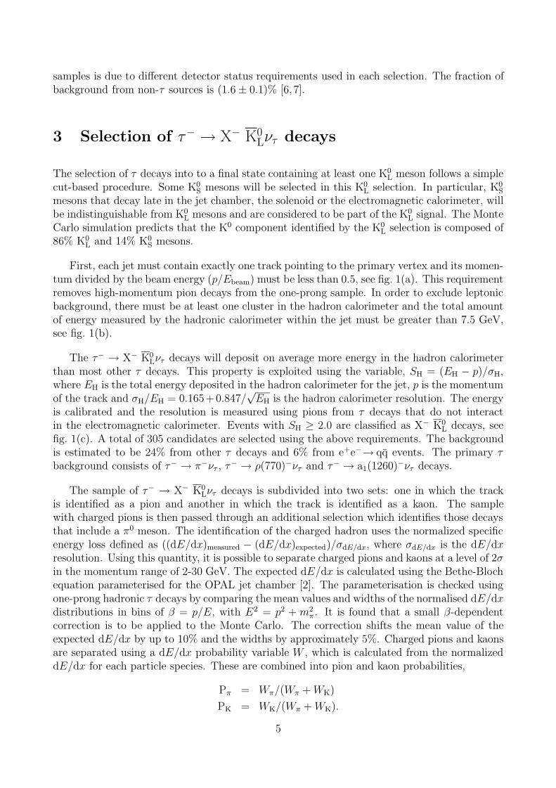
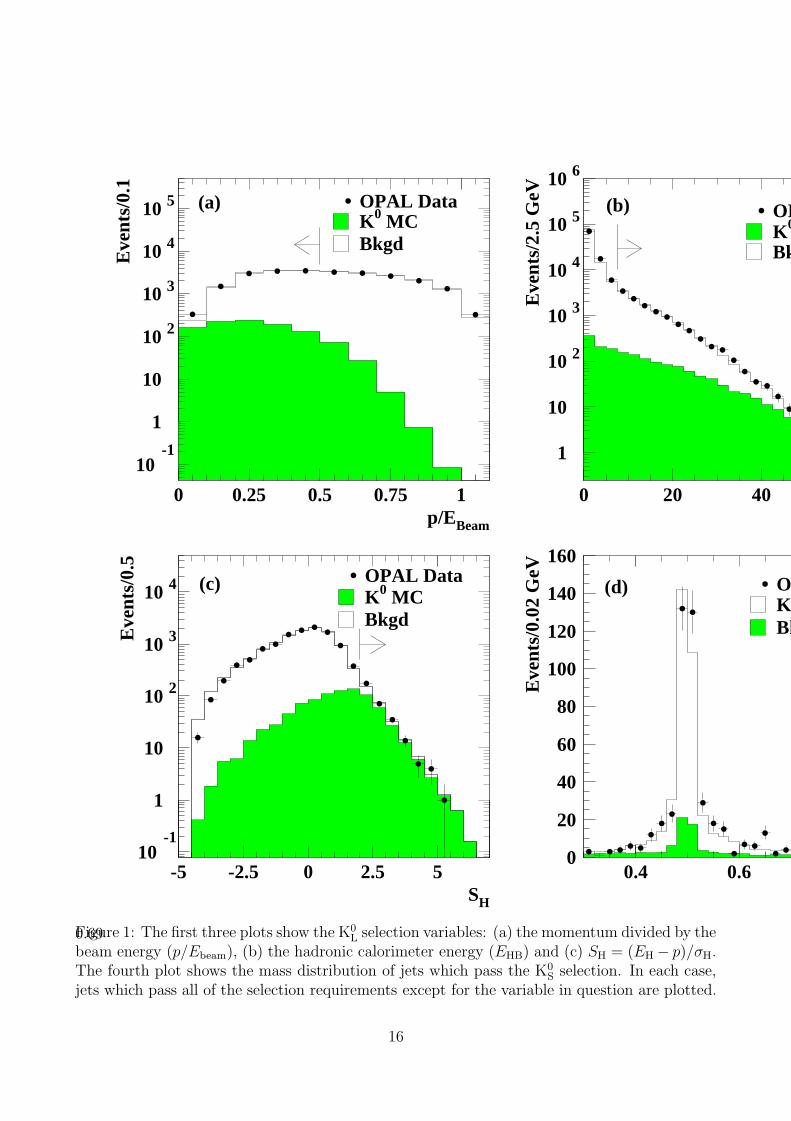
First, each jet must contain exactly one track pointing to the primary vertex and its momen-tum divided by the beam energy (p/Ebeam) must be less than 0.5, see fig. 1(a). This requirementremoves high-momentum pion decays from the one-prong sample. In order to exclude leptonicbackground, there must be at least one cluster in the hadron calorimeter and the total amountof energy measured by the hadronic calorimeter within the jet must be greater than 7.5 GeV,see fig. 1(b).

The τ− → X− K0Lντ decays will deposit on average more energy in the hadron calorimeter

than most other τ decays. This property is exploited using the variable, SH = (EH − p)/σH,where EH is the total energy deposited in the hadron calorimeter for the jet, p is the momentumof the track and σH/EH = 0.165+0.847/

√EH is the hadron calorimeter resolution. The energy

is calibrated and the resolution is measured using pions from τ decays that do not interactin the electromagnetic calorimeter. Events with SH ≥ 2.0 are classified as X− K0

L decays, seefig. 1(c). A total of 305 candidates are selected using the above requirements. The backgroundis estimated to be 24% from other τ decays and 6% from e+e−→ qq events. The primary τbackground consists of τ− → π−ντ , τ− → ρ(770)−ντ and τ− → a1(1260)−ντ decays.

The sample of τ− → X− K0Lντ decays is subdivided into two sets: one in which the track

is identified as a pion and another in which the track is identified as a kaon. The samplewith charged pions is then passed through an additional selection which identifies those decaysthat include a π0 meson. The identification of the charged hadron uses the normalized specificenergy loss defined as ((dE/dx)measured − (dE/dx)expected)/σdE/dx, where σdE/dx is the dE/dxresolution. Using this quantity, it is possible to separate charged pions and kaons at a level of 2σin the momentum range of 2-30 GeV. The expected dE/dx is calculated using the Bethe-Blochequation parameterised for the OPAL jet chamber [2]. The parameterisation is checked usingone-prong hadronic τ decays by comparing the mean values and widths of the normalised dE/dxdistributions in bins of β = p/E, with E2 = p2 + m2

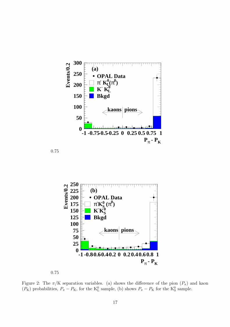
π. It is found that a small β-dependentcorrection is to be applied to the Monte Carlo. The correction shifts the mean value of theexpected dE/dx by up to 10% and the widths by approximately 5%. Charged pions and kaonsare separated using a dE/dx probability variable W , which is calculated from the normalizeddE/dx for each particle species. These are combined into pion and kaon probabilities,

Pπ = Wπ/(Wπ + WK)

PK = WK/(Wπ + WK).

5

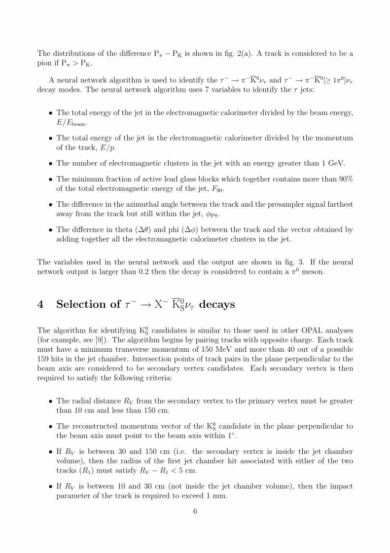
The distributions of the difference Pπ − PK is shown in fig. 2(a). A track is considered to be apion if Pπ > PK.

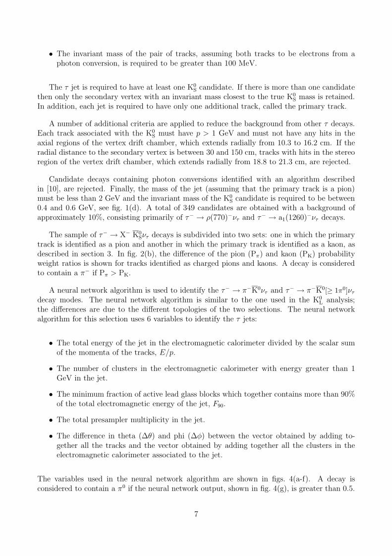
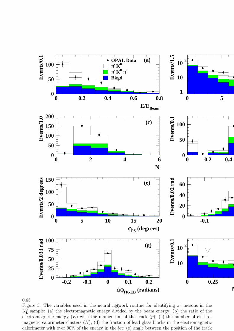
A neural network algorithm is used to identify the τ− → π−K0ντ and τ− → π−K0[≥ 1π0]ντ

decay modes. The neural network algorithm uses 7 variables to identify the τ jets:

• The total energy of the jet in the electromagnetic calorimeter divided by the beam energy,E/Ebeam.

• The total energy of the jet in the electromagnetic calorimeter divided by the momentumof the track, E/p.

• The number of electromagnetic clusters in the jet with an energy greater than 1 GeV.

• The minimum fraction of active lead glass blocks which together contains more than 90%of the total electromagnetic energy of the jet, F90.

• The difference in the azimuthal angle between the track and the presampler signal farthestaway from the track but still within the jet, φPS.

• The difference in theta (∆θ) and phi (∆φ) between the track and the vector obtained byadding together all the electromagnetic calorimeter clusters in the jet.

The variables used in the neural network and the output are shown in fig. 3. If the neuralnetwork output is larger than 0.2 then the decay is considered to contain a π0 meson.

4 Selection of τ− → X− K0Sντ decays

The algorithm for identifying K0S candidates is similar to those used in other OPAL analyses

(for example, see [9]). The algorithm begins by pairing tracks with opposite charge. Each trackmust have a minimum transverse momentum of 150 MeV and more than 40 out of a possible159 hits in the jet chamber. Intersection points of track pairs in the plane perpendicular to thebeam axis are considered to be secondary vertex candidates. Each secondary vertex is thenrequired to satisfy the following criteria:

• The radial distance RV from the secondary vertex to the primary vertex must be greaterthan 10 cm and less than 150 cm.

• The reconstructed momentum vector of the K0S candidate in the plane perpendicular to

the beam axis must point to the beam axis within 1◦.

• If RV is between 30 and 150 cm (i.e. the secondary vertex is inside the jet chambervolume), then the radius of the first jet chamber hit associated with either of the twotracks (R1) must satisfy RV −R1 < 5 cm.

• If RV is between 10 and 30 cm (not inside the jet chamber volume), then the impactparameter of the track is required to exceed 1 mm.

6

• The invariant mass of the pair of tracks, assuming both tracks to be electrons from aphoton conversion, is required to be greater than 100 MeV.

The τ jet is required to have at least one K0S candidate. If there is more than one candidate

then only the secondary vertex with an invariant mass closest to the true K0S mass is retained.

In addition, each jet is required to have only one additional track, called the primary track.

A number of additional criteria are applied to reduce the background from other τ decays.Each track associated with the K0

S must have p > 1 GeV and must not have any hits in theaxial regions of the vertex drift chamber, which extends radially from 10.3 to 16.2 cm. If theradial distance to the secondary vertex is between 30 and 150 cm, tracks with hits in the stereoregion of the vertex drift chamber, which extends radially from 18.8 to 21.3 cm, are rejected.

Candidate decays containing photon conversions identified with an algorithm describedin [10], are rejected. Finally, the mass of the jet (assuming that the primary track is a pion)must be less than 2 GeV and the invariant mass of the K0

S candidate is required to be between0.4 and 0.6 GeV, see fig. 1(d). A total of 349 candidates are obtained with a background ofapproximately 10%, consisting primarily of τ− → ρ(770)−ντ and τ− → a1(1260)−ντ decays.

The sample of τ− → X− K0Sντ decays is subdivided into two sets: one in which the primary

track is identified as a pion and another in which the primary track is identified as a kaon, asdescribed in section 3. In fig. 2(b), the difference of the pion (Pπ) and kaon (PK) probabilityweight ratios is shown for tracks identified as charged pions and kaons. A decay is consideredto contain a π− if Pπ > PK.

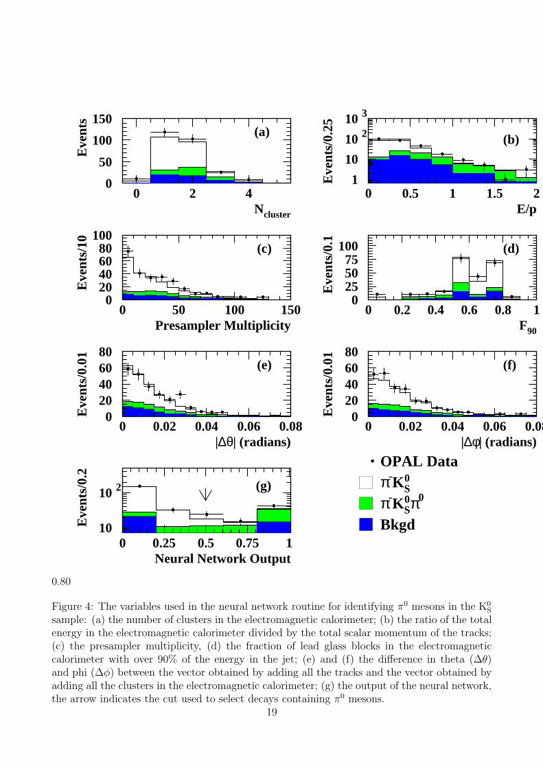
A neural network algorithm is used to identify the τ− → π−K0ντ and τ− → π−K0[≥ 1π0]ντ

decay modes. The neural network algorithm is similar to the one used in the K0L analysis;

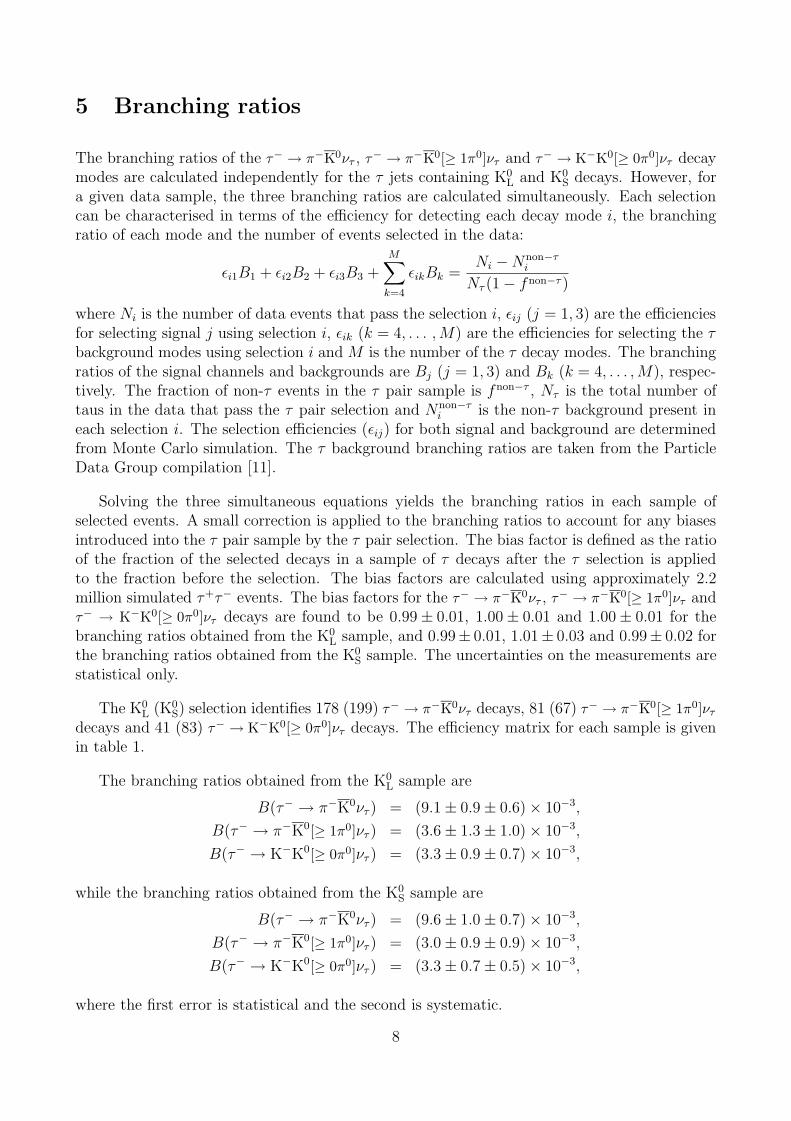
the differences are due to the different topologies of the two selections. The neural networkalgorithm for this selection uses 6 variables to identify the τ jets:

• The total energy of the jet in the electromagnetic calorimeter divided by the scalar sumof the momenta of the tracks, E/p.

• The number of clusters in the electromagnetic calorimeter with energy greater than 1GeV in the jet.

• The minimum fraction of active lead glass blocks which together contains more than 90%of the total electromagnetic energy of the jet, F90.

• The total presampler multiplicity in the jet.

• The difference in theta (∆θ) and phi (∆φ) between the vector obtained by adding to-gether all the tracks and the vector obtained by adding together all the clusters in theelectromagnetic calorimeter associated to the jet.

The variables used in the neural network algorithm are shown in figs. 4(a-f). A decay isconsidered to contain a π0 if the neural network output, shown in fig. 4(g), is greater than 0.5.

7

5 Branching ratios

The branching ratios of the τ− → π−K0ντ , τ− → π−K0[≥ 1π0]ντ and τ− → K−K0[≥ 0π0]ντ decaymodes are calculated independently for the τ jets containing K0

L and K0S decays. However, for

a given data sample, the three branching ratios are calculated simultaneously. Each selectioncan be characterised in terms of the efficiency for detecting each decay mode i, the branchingratio of each mode and the number of events selected in the data:

εi1B1 + εi2B2 + εi3B3 +

M∑k=4

εikBk =Ni −Nnon−τ

i

Nτ (1− fnon−τ )

where Ni is the number of data events that pass the selection i, εij (j = 1, 3) are the efficienciesfor selecting signal j using selection i, εik (k = 4, . . . , M) are the efficiencies for selecting the τbackground modes using selection i and M is the number of the τ decay modes. The branchingratios of the signal channels and backgrounds are Bj (j = 1, 3) and Bk (k = 4, . . . , M), respec-tively. The fraction of non-τ events in the τ pair sample is fnon−τ , Nτ is the total number oftaus in the data that pass the τ pair selection and Nnon−τ

i is the non-τ background present ineach selection i. The selection efficiencies (εij) for both signal and background are determinedfrom Monte Carlo simulation. The τ background branching ratios are taken from the ParticleData Group compilation [11].

Solving the three simultaneous equations yields the branching ratios in each sample ofselected events. A small correction is applied to the branching ratios to account for any biasesintroduced into the τ pair sample by the τ pair selection. The bias factor is defined as the ratioof the fraction of the selected decays in a sample of τ decays after the τ selection is appliedto the fraction before the selection. The bias factors are calculated using approximately 2.2million simulated τ+τ− events. The bias factors for the τ− → π−K0ντ , τ− → π−K0[≥ 1π0]ντ andτ− → K−K0[≥ 0π0]ντ decays are found to be 0.99± 0.01, 1.00± 0.01 and 1.00± 0.01 for thebranching ratios obtained from the K0

L sample, and 0.99± 0.01, 1.01± 0.03 and 0.99± 0.02 forthe branching ratios obtained from the K0

S sample. The uncertainties on the measurements arestatistical only.

The K0L (K0

S) selection identifies 178 (199) τ− → π−K0ντ decays, 81 (67) τ− → π−K0[≥ 1π0]ντ

decays and 41 (83) τ− → K−K0[≥ 0π0]ντ decays. The efficiency matrix for each sample is givenin table 1.

The branching ratios obtained from the K0L sample are

B(τ− → π−K0ντ ) = (9.1± 0.9± 0.6)× 10−3,

B(τ− → π−K0[≥ 1π0]ντ ) = (3.6± 1.3± 1.0)× 10−3,

B(τ− → K−K0[≥ 0π0]ντ ) = (3.3± 0.9± 0.7)× 10−3,

while the branching ratios obtained from the K0S sample are

B(τ− → π−K0ντ ) = (9.6± 1.0± 0.7)× 10−3,

B(τ− → π−K0[≥ 1π0]ντ ) = (3.0± 0.9± 0.9)× 10−3,

B(τ− → K−K0[≥ 0π0]ντ ) = (3.3± 0.7± 0.5)× 10−3,

where the first error is statistical and the second is systematic.

8

6 Systematic errors

The systematic uncertainties on the branching ratios are presented in table 2. The dominantcontributions to the systematic uncertainty arises from the efficiency of the two selections, theuncertainty of the backgrounds, the modelling of the dE/dx, the identification of the π0 and themodelling of Monte Carlo. These uncertainties are discussed in more detail below. In addition,there are straightforward contributions from the limited statistics of the Monte Carlo samplesused to estimate the selection efficiencies and from the uncertainties on the bias factors. Thesystematic error on the branching ratios due to the Monte Carlo statistics is calculated directlyfrom the statistical uncertainties on the elements of the inverse efficiency matrix [12]. Thesystematic error on each branching ratio due to the bias factor is calculated directly from thebias factor error.

K0L and K0

S selection efficiencies:

The K0L selection efficiency is sensitive to the calibration of the momentum, the energy measured

by the hadron calorimeter and the resolution of the hadron calorimeter. The uncertainty onthe momentum scale is typically better than 1% [7]. The uncertainty in the energy scale of thehadron calorimeter is obtained by studying a sample of single charged hadrons from τ decays,the level of agreement between the data and Monte Carlo is 1.5%. The uncertainty due to themeasurement of the resolution of the hadron calorimeter is estimated by varying the resolutionwithin its uncertainties. Also, the shower containment is examined by looking at the leakageof energy out of the back of the hadron calorimeter. It is found that about 8% of K0

L decaysmay not be fully contained, these decays are well modelled by the Monte Carlo and does notresult in a systematic uncertainty.

The K0S selection efficiency is sensitive to the requirements on the impact parameter, the

momentum and the number of hits in the stereo and axial regions of the vertex chamberon the tracks associated to the K0

S . The systematic error on the K0S selection efficiency is

determined by dropping each relevant criterion except for the impact parameter resolution.The impact parameter resolution has been shown to have an uncertainty that is typicallybetter than ±20% [8]. Variations of the impact parameter resolution are found to have almostno contribution to the systematic error on the K0

S selection efficiency.

Background estimation:

The systematic error due to the background in the K0L sample includes the uncertainty in the

branching ratios of the background decays, including the τ− → π−K0K0ντ and τ− → π−K0K0π0ντ

decays, as well as the uncertainty from the Monte Carlo statistics [11, 13]. The non-K0 back-ground consists primarily of π−, ρ(770)− and a1(1260)− decays in which the decays have a lowmomentum track with at least one of the final π mesons leaving some energy in the hadroncalorimeter. To investigate this background, the K0

L selection cut SH is reversed and the in-variant mass spectra are studied for each decay mode. The ratios of the data to the MonteCarlo simulation are consistent with unity: 0.97 ± 0.02, 1.04 ± 0.02 and 0.94 ± 0.06 for theπ−K0, π−K0 ≥ 1π0 and K−K0 ≥ 0π0 selections, respectively. The various contributions to thesystematic error from the background are added in quadrature.

The background in the K0S sample includes τ− → π−K0K0ντ and τ− → π−K0K0π0ντ decays,

9

which contain K0S mesons, and other τ decays, the uncertainty is composed of the Monte Carlo

statistical uncertainty plus a component due to the uncertainty in the branching ratios of thesedecays [11, 13]. A study of the sidebands of the mππ distribution (see fig. 1(d)) showed thatthe background prediction from other τ decays is observed to be about 20% smaller in theMonte Carlo simulation than in the data. As a result, the background is scaled upward by afactor of 1.2 and a 20% uncertainty is assigned to the background estimate. The backgroundestimate is cross-checked using the invariant mass distributions of the tracks associated withthe K0

S candidate for each of the exclusive channels. The ratios of the data to the Monte Carlosimulation are consistent: 1.07 ± 0.12, 1.09 ± 0.06 and 0.93 ± 0.11 for the π−K0

S, π−K0S ≥ 1π0

and K−K0S ≥ 0π0 selections, respectively. The various contributions to the systematic error

from the background are added in quadrature.

Modelling of dE/dx:

For both samples, the normalized dE/dx distributions are studied using the sample of singlecharged hadrons from τ decays. The uncertainty in the branching ratios is estimated by varyingthe means of the normalised dE/dx distributions by ±1 standard deviation of their centralvalues. In addition, to account for possible differences in the dE/dx resolution, the widths ofthe normalized dE/dx distributions are varied by ±30%. Due to the three tracks present inthe K0

S sample, an additional contribution to the systematic error is obtained by measuringthe difference in the branching ratios when two different corrections are applied to the MonteCarlo. The first correction is estimated from the one-prong hadronic tau decays while thesecond correction is estimated using the sample of pions from the decay of the K0

S. The variouscontributions to the systematic error from the dE/dx modelling are added in quadrature.

Identification of π0:

Both the K0L and K0

S samples use a neural network algorithm to separate the τ− → π−K0ντ

and τ− → π−K0[≥ 1π0]ντ decay modes. The most powerful variable for distinguishing betweenthese two decays is the energy deposited in the electromagnetic calorimeter. The systematicerror in the branching ratio is evaluated by shifting the electromagnetic energy scale by ±1%;this variation is assigned after studying the differences between data and Monte Carlo in E/pdistributions for 3-prong τ decays.

The uncertainty affecting the π0 identification also includes the maximum uncertainty wheneach variable (except in those which include the electromagnetic energy) is individually droppedfrom the neural network algorithm. These uncertainties are added in quadrature with thoseobtained from the energy scale uncertainty. The stability of the neural network algorithm isstudied by removing all but the two most significant variables from the neural network, theresults are within the systematic uncertainties for both samples. As a cross check, the cut onthe neural network output for both the K0

L and K0S samples is varied between 0.1 and 0.8, with

the result being consistent within the total systematic uncertainties.

Monte Carlo modelling:

The models used in the Monte Carlo generator can effect both the pion and kaon momentumspectra. This effect can produce biases when determining the K0 identification efficiency, theK/π separation and the π0 identification. The dynamics of the π−K0 decay mode are wellunderstood. The π−K0 decay mode is generated by Tauola via the K∗(892)− resonance. The

10

K−K0 final state is generated by Tauola using phase space only.

The τ− → π−K0[≥ 1π0]ντ decay mode is composed of τ−→ π−K0π0ντ and τ−→π−K0π0π0ντ

decays. The τ− → π−K0π0ντ channel is modelled by Tauola assuming that the decay proceedsvia the K1(1400) resonance. Recent results from ALEPH [14] on one-prong τ decays with kaons,and OPAL [15] using τ− → K−π−π+ντ decays, suggest that the τ− → π−K0π0ντ decay will alsoproceed via the K1(1270) resonance. A special Monte Carlo simulation is generated in whichthe final state is created using the K1(1270) and K1(1400) resonances, using the algorithmdeveloped for the analysis described in [15]. The selection efficiency of the τ− → π−K0π0ντ

final state is estimated from the special Monte Carlo for both resonances. For the K0L analysis,

the efficiencies agree at a level of 10%. For the K0S analysis, the selection efficiencies agree at a

level of 5%.

The τ− → π−K0π0π0ντ decay mode is not modelled by Tauola. The branching ratio of thismode was recently measured to be (0.26 ± 0.24) × 10−3 [13]. A special Monte Carlo sampleof the τ− → π−K0π0π0ντ decay mode is generated using flat phase space and it is found thatthe efficiency of the τ− → π−K0π0π0ντ decay mode agrees within 30% of the efficiency of theτ− → π−K0π0ντ decay mode. For the systematic uncertainty associated with this decay mode,30% of the τ− → π−K0π0π0ντ branching ratio is used.

The τ− → K−K0[≥ 1π0]ντ decay mode is composed of τ− → K−K0π0ντ and τ− →K−K0π0π0ντ decays. The τ− → K−K0π0ντ decay mode is generated by Tauola through acombination of the ρ(1700) and a1(1260) resonances. Monte Carlo simulations of these twomodes are generated separately, again using the algorithm developed for the analysis describedin [15]. The selection efficiencies of the τ− → K−K0π0ντ decay mode are calculated for thesetwo samples and are equivalent within statistical errors. No systematic uncertainty is includedfor this channel. The τ− → K−K0π0π0ντ decay mode is not modelled by Tauola. The ParticleData Group [11] give an upper bound of 0.18 × 10−3 for this channel. A special Monte Carlosample of the τ− → K−K0π0π0ντ decay mode is generated using flat phase space and the effi-ciency of the τ− → K−K0π0π0ντ decay mode is observed to be within 30% of the efficiency ofthe τ− → K−K0π0ντ decay mode. For the systematic uncertainty associated with this decaymode, 30% of the τ− → K−K0π0π0ντ branching ratio is used.

Finally, the τ− → K−K0[≥ 1π0]ντ selection efficiency may depend on the relative τ− →K−K0ντ and τ− → K−K0π0ντ branching ratios. Using the current world averages from [11],the relative contribution of each channel is varied by ±25%. For the K0

S analysis, no effect isobserved on the branching ratio, as the efficiency for selecting the two channels is very similar;hence, no systematic error is included.

7 Summary

The branching ratios of the decays of the τ leptons to neutral kaons are measured using theOPAL data recorded at centre-of-mass energies near the Z0 resonance from a recorded lumi-nosity of 163 pb−1. The measurement is based on two samples which identify τ decays with K0

L

11

and K0S mesons. The branching ratios obtained from the K0

L sample are

B(τ− → π−K0ντ ) = (9.1± 0.9± 0.6)× 10−3,

B(τ− → π−K0[≥ 1π0]ντ ) = (3.6± 1.3± 1.0)× 10−3,

B(τ− → K−K0[≥ 0π0]ντ ) = (3.3± 0.9± 0.7)× 10−3,

while the branching ratios obtained from the K0S sample are

B(τ− → π−K0ντ ) = (9.6± 1.0± 0.7)× 10−3,

B(τ− → π−K0[≥ 1π0]ντ ) = (3.0± 0.9± 0.9)× 10−3,

B(τ− → K−K0[≥ 0π0]ντ ) = (3.3± 0.7± 0.5)× 10−3.

In each case the first error is statistical and the second systematic. The combined results are

B(τ− → π−K0ντ ) = (9.33± 0.68± 0.49)× 10−3,

B(τ− → π−K0[≥ 1π0]ντ ) = (3.24± 0.74± 0.66)× 10−3,

B(τ− → K−K0[≥ 0π0]ντ ) = (3.30± 0.55± 0.39)× 10−3.

The branching ratios are compared with existing measurements and theoretical predictions infig. 5 for the τ− → π−K0ντ and τ− → π−K0[≥ 1π0]ντ decay modes [14, 16]. The solid bandis the new average branching ratio of the OPAL, ALEPH, CLEO and L3 measurements. Theresults of this work are in good agreement with previous measurements.

The branching ratios of the decay modes are predicted from various theoretical models.The measurement of the decay fraction of the τ− → π−K0ντ decay agrees well with the range(8.9−10.3)×10−3 estimated by Braaten et al. in [17] and falls in the range of (6.6−9.6)×10−3

predicted by Finkemeier and Mirkes in [18]. The decay τ− → π−K0[≥ 1π0]ντ , assuming thatthe decay contains only one π0, is predicted to be in the range of (0.9 − 3.7)× 10−3 from [17]and in the range of (8.1−9.6)×10−3 from [18]. The τ− → π−K0π0ντ branching ratio predictionby Finkemeier and Mirkes is significantly higher than the experimental results, however theyargue that the widths of the K1 resonance [11] used in their calculation are unusually narrowand that increasing the K1 width would give a prediction that agrees with the experimentalmeasurements [19].

The branching ratio of the τ− → K−K0[≥ 0π0]ντ decay mode is the sum of the τ− → K−K0ντ

and τ− → K−K0π0ντ decay modes. The decay fraction agrees well with the estimated range(2.4− 4.0)× 10−3 predicted by [17] and (2.3− 2.7)× 10−3 predicted by [18].

The τ− → π−K0ντ decay mode is assumed to be dominated by the K∗(892)− resonance. This

can be observed from the π−K0

invariant mass distributions shown in fig. 6, for the decay modesτ− → π−K0

Sντ and τ− → π−K0Lντ , respectively. Assuming that the τ− → π−K0ντ decay mode

proceeds entirely through the K∗(892)− resonance, then using isospin invariance the branchingratio of the τ− → K∗(892)−ντ decay mode is calculated to be 0.0140 ± 0.0013. This value isconsistent with the current world average 0.0128± 0.0008 [11].

Finally, the ratio of the decay constants fρ and fK∗ can be estimated using the τ− →K∗(892)−ντ branching ratio and the OPAL τ− → h−π0ντ branching ratio of 0.2589±0.0034 [7].The τ− → h−π0ντ decay mode is the sum of the decay modes τ− → π−π0ντ and τ− → K−π0ντ .

12

The branching ratio of the τ to the final state K−π0ντ is calculated to be (4.67± 0.42)× 10−3

using isospin invariance and the τ− → π−K0ντ branching ratio. Consequently, B(τ− → π−π0ντ )is derived to be 0.2543± 0.0034. Using these results, tan θc = 0.227 for the Cabibbo angle andthe particle masses from [11], the decay constant ratio

fρ

fK∗= tan θc

√B(τ− → ρ−ντ )

B(τ− → K∗(892)−ντ )

(m2

τ −m2K∗

m2τ −m2

ρ

) √m2

τ + 2m2K∗

m2τ + 2m2

ρ

= 0.93± 0.05

is obtained. The error is dominated by the uncertainties on the branching ratios. The recentresult from ALEPH [13], 0.94± 0.03, agrees well with the new OPAL result. Finally, this ratiohas been predicted by Oneda [20] using the Das-Mathur-Okubo sum rule relations [21] betweenthe spectral functions based on assumptions of SU(3)f symmetry. At the SU(3)f symmetrylimit (mu = md = ms), the decay constant ratio is expected to be unity, fρ = fK∗ . In theasymptotic SU(3)f symmetry limit at high energies, Oneda predicts that fρ/fK∗ = mρ/mK∗ =0.86.

Acknowledgements

We particularly wish to thank the SL Division for the efficient operation of the LEP acceleratorat all energies and for their continuing close cooperation with our experimental group. Wethank our colleagues from CEA, DAPNIA/SPP, CE-Saclay for their efforts over the years onthe time-of-flight and trigger systems which we continue to use. In addition to the support staffat our own institutions we are pleased to acknowledge theDepartment of Energy, USA,National Science Foundation, USA,Particle Physics and Astronomy Research Council, UK,Natural Sciences and Engineering Research Council, Canada,Israel Science Foundation, administered by the Israel Academy of Science and Humanities,Minerva Gesellschaft,Benoziyo Center for High Energy Physics,Japanese Ministry of Education, Science and Culture (the Monbusho) and a grant under theMonbusho International Science Research Program,Japanese Society for the Promotion of Science (JSPS),German Israeli Bi-national Science Foundation (GIF),Bundesministerium fur Bildung, Wissenschaft, Forschung und Technologie, Germany,National Research Council of Canada,Research Corporation, USA,Hungarian Foundation for Scientific Research, OTKA T-029328, T023793 and OTKA F-023259.

13

References

[1] OPAL Collaboration, K. Ahmet et al., Nucl. Instr. and Meth. A305 (1991) 275;P.P. Allport et al., Nucl. Instr. and Meth. A324 (1993) 34;P.P. Allport et al., Nucl. Instr. and Meth. A346 (1994) 476.

[2] M. Hauschild et al., Nucl. Instr. and Meth. A314 (1992) 74;O. Biebel et al., Nucl. Instr. and Meth. A323 (1992) 169;M. Hauschild, Nucl. Instr. and Meth. A379 (1996) 436.

[3] S. Jadach, B.F.L. Ward, and Z. Was, Comp. Phys. Comm. 79 (1994) 503.

[4] S. Jadach et al., Comp. Phys. Comm. 76 (1993) 361.

[5] J. Allison et al., Nucl. Inst. and Meth. A317 (1992) 47.

[6] OPAL Collaboration, G. Alexander et al., Phys. Lett. B369 (1996) 163.

[7] OPAL Collaboration, K. Ackerstaff et al., Eur. Phys. J. C4 (1998) 193.

[8] OPAL Collaboration, K. Ackerstaff et al., Eur. Phys. J. C8 (1999) 183.

[9] OPAL Collaboration, R. Akers et al., Z. Phys. C67 (1995) 389.

[10] OPAL Collaboration, G. Alexander et al., Z. Phys. C70 (1996) 357.

[11] Particle Data Group, C. Caso et al., Eur. Phys. J. C3 (1998) 1.

[12] M. Lefebvre, R.K. Keeler, R. Sobie and J. White, Propagation of Errors for Matrix Inver-sion, hep-ex/9909031, Submitted to Nucl. Inst. and Meth.

[13] ALEPH Collaboration, R. Barate et al., Study of Tau Decays Involving Kaons, SpectralFunctions and Determination of the Strange Quark Mass, CERN-EP/99-026.

[14] ALEPH Collaboration, R. Barate et al., Eur. Phys. J., C10 (1999) 1.

[15] OPAL Collaboration, G. Abbiendi et al., A Study of three Prong Tau Decays with ChargedKaons, CERN-EP/99-095.

[16] ALEPH Collaboration, R. Barate et al., Eur. Phys. J., C4 (1998) 29;L3 Collaboration, M. Acciarri et al., Phys. Lett. B352 (1995) 487;CLEO Collaboration, T.E. Coan et al., Phys. Rev. D53 (1996) 6037.

[17] E. Braaten, R. Oakes and S. Tse, Int. J. Mod. Phys., A5 (1990) 2737.

[18] M. Finkemeier and E. Mirkes, Z.Phys., C69 (1996) 243.

[19] M. Finkemeier, J.H. Kuhn and E. Mirkes, Nucl. Phys. Proc. Suppl. C55 (1997) 169.

[20] S. Oneda, Phys. Rev. D35 (1987) 397;T. Matsuda and S. Oneda, Phys. Rev. 171 (1968) 1743.

[21] T. Das, V.S. Mathur and S. Okubo, Phys. Rev. Lett. 18 (1967) 761;T. Das, V.S. Mathur and S. Okubo, Phys. Rev. Lett. 19 (1967) 859.

14

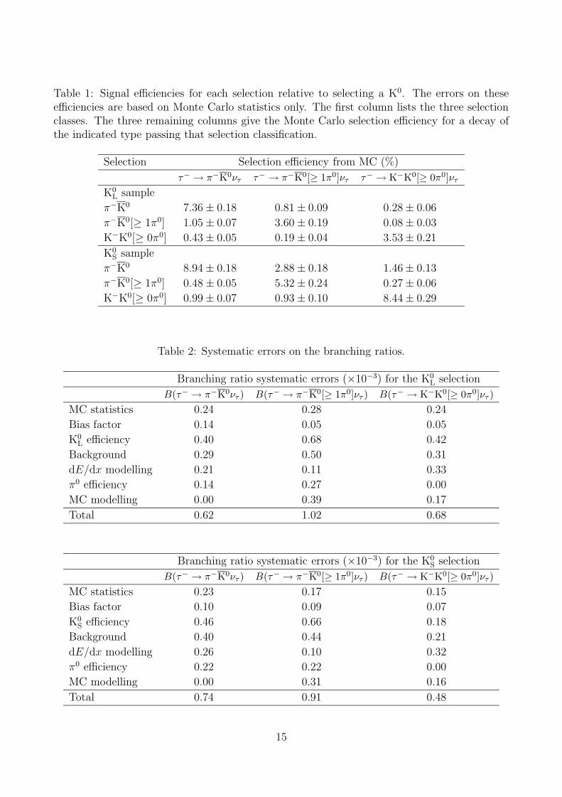
Table 1: Signal efficiencies for each selection relative to selecting a K0. The errors on theseefficiencies are based on Monte Carlo statistics only. The first column lists the three selectionclasses. The three remaining columns give the Monte Carlo selection efficiency for a decay ofthe indicated type passing that selection classification.

Selection Selection efficiency from MC (%)

τ− → π−K0ντ τ− → π−K0[≥ 1π0]ντ τ− → K−K0[≥ 0π0]ντ

K0L sample

π−K0 7.36± 0.18 0.81± 0.09 0.28± 0.06

π−K0[≥ 1π0] 1.05± 0.07 3.60± 0.19 0.08± 0.03

K−K0[≥ 0π0] 0.43± 0.05 0.19± 0.04 3.53± 0.21

K0S sample

π−K0 8.94± 0.18 2.88± 0.18 1.46± 0.13

π−K0[≥ 1π0] 0.48± 0.05 5.32± 0.24 0.27± 0.06

K−K0[≥ 0π0] 0.99± 0.07 0.93± 0.10 8.44± 0.29

Table 2: Systematic errors on the branching ratios.

Branching ratio systematic errors (×10−3) for the K0L selection

B(τ− → π−K0ντ ) B(τ− → π−K0[≥ 1π0]ντ ) B(τ− → K−K0[≥ 0π0]ντ )MC statistics 0.24 0.28 0.24

Bias factor 0.14 0.05 0.05

K0L efficiency 0.40 0.68 0.42

Background 0.29 0.50 0.31

dE/dx modelling 0.21 0.11 0.33

π0 efficiency 0.14 0.27 0.00

MC modelling 0.00 0.39 0.17

Total 0.62 1.02 0.68

Branching ratio systematic errors (×10−3) for the K0S selection

B(τ− → π−K0ντ ) B(τ− → π−K0[≥ 1π0]ντ ) B(τ− → K−K0[≥ 0π0]ντ )MC statistics 0.23 0.17 0.15

Bias factor 0.10 0.09 0.07

K0S efficiency 0.46 0.66 0.18

Background 0.40 0.44 0.21

dE/dx modelling 0.26 0.10 0.32

π0 efficiency 0.22 0.22 0.00

MC modelling 0.00 0.31 0.16

Total 0.74 0.91 0.48

15

0.69

10-1

1

10

10 2

10 3

10 4

10 5

0 0.25 0.5 0.75 1p/EBeam

Eve

nts/

0.1

(a) OPAL Data

BkgdK0 MC

1

10

10 2

10 3

10 4

10 5

10 6

0 20 40

Eve

nts/

2.5

GeV

(b) OP

BkK0

10-1

1

10

10 2

10 3

10 4

-5 -2.5 0 2.5 5SH

Eve

nts/

0.5

(c) OPAL Data

BkgdK0 MC

0

20

40

60

80

100

120

140

160

0.4 0.6

Eve

nts/

0.02

GeV

(d) OPKS

0

Bk

Figure 1: The first three plots show the K0L selection variables: (a) the momentum divided by the

beam energy (p/Ebeam), (b) the hadronic calorimeter energy (EHB) and (c) SH = (EH− p)/σH.The fourth plot shows the mass distribution of jets which pass the K0

S selection. In each case,jets which pass all of the selection requirements except for the variable in question are plotted.

16

0.75

0

50

100

150

200

250

300

-1 -0.75-0.5-0.25 0 0.25 0.5 0.75 1Pπ - PK

Eve

nts/

0.2

(a)OPAL Dataπ- K0

L(π0)K- K0

LBkgd

pionskaons

0.75

0255075

100125150175200225250

-1 -0.8-0.6-0.4-0.2 0 0.20.40.60.8 1

(b)

Pπ - PK

Eve

nts/

0.2

OPAL Dataπ-KS

0 (π0)K-KS

0

Bkgd

pionskaons

Figure 2: The π/K separation variables. (a) shows the difference of the pion (Pπ) and kaon(PK) probabilities, Pπ − PK, for the K0

L sample, (b) shows Pπ − PK for the K0S sample.

17

0.65

0

50

100

0 0.2 0.4 0.6 0.8E/EBeam

Eve

nts/

0.1

(a)OPAL Dataπ- K0

π- K0 π0

Bkgd

1

10

10 2

0 5

Eve

nts/

1.5

0

50

100

150

200

0 2 4 6N

Eve

nts/

1.0

(c)

0

50

100

0 0.2 0.4

Eve

nts/

0.1

0

50

100

150

0 5 10 15 20φPS (degrees)

Eve

nts/

2 de

gree

s

(e)

0

20

40

60

-0.1

Eve

nts/

0.02

rad

0

25

50

75

100

-0.2 -0.1 0 0.1 0.2∆φTK-EB (radians)

Eve

nts/

0.03

3 ra

d

(g)

10

10 2

0 0.25N

Eve

nts/

0.1

Figure 3: The variables used in the neural network routine for identifying π0 mesons in theK0

L sample: (a) the electromagnetic energy divided by the beam energy; (b) the ratio of theelectromagnetic energy (E) with the momentum of the track (p); (c) the number of electro-magnetic calorimeter clusters (N); (d) the fraction of lead glass blocks in the electromagneticcalorimeter with over 90% of the energy in the jet; (e) angle between the position of the track

18

0.80

(a)

Ncluster

Eve

nts

(b)

E/p

Eve

nts/

0.25

Presampler Multiplicity

Eve

nts/

10 (c) (d)

F90E

vent

s/0.

1

(e)

|∆θ| (radians)

Eve

nts/

0.01

(f)

|∆φ| (radians)

Eve

nts/

0.01

(g)

Neural Network Output

Eve

nts/

0.2 OPAL Data

π-KS0

π-KS0π0

Bkgd

0

50

100

150

0 2 41

10

10 210 3

0 0.5 1 1.5 2

020406080

100

0 50 100 1500

255075

100

0 0.2 0.4 0.6 0.8 1

020406080

0 0.02 0.04 0.06 0.080

20406080

0 0.02 0.04 0.06 0.08

10

10 2

0 0.25 0.5 0.75 1

Figure 4: The variables used in the neural network routine for identifying π0 mesons in the K0S

sample: (a) the number of clusters in the electromagnetic calorimeter; (b) the ratio of the totalenergy in the electromagnetic calorimeter divided by the total scalar momentum of the tracks;(c) the presampler multiplicity, (d) the fraction of lead glass blocks in the electromagneticcalorimeter with over 90% of the energy in the jet; (e) and (f) the difference in theta (∆θ)and phi (∆φ) between the vector obtained by adding all the tracks and the vector obtained byadding all the clusters in the electromagnetic calorimeter; (g) the output of the neural network,the arrow indicates the cut used to select decays containing π0 mesons.

19

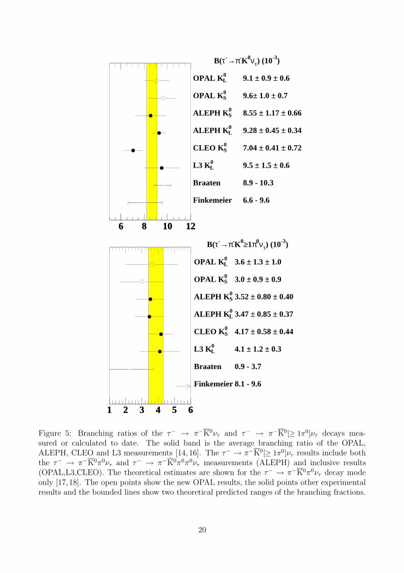
6 8 10 126 8 10 12

OPAL K 0L 9.1 ± 0.9 ± 0.6

OPAL K 0S 9.6± 1.0 ± 0.7

ALEPH K 0S 8.55 ± 1.17 ± 0.66

ALEPH K 0L 9.28 ± 0.45 ± 0.34

CLEO K 0S 7.04 ± 0.41 ± 0.72

L3 K 0L 9.5 ± 1.5 ± 0.6

Braaten 8.9 - 10.3

Finkemeier 6.6 - 9.6

B(τ-→π-K0ντ) (10-3)

1 2 3 4 5 61 2 3 4 5 6

OPAL K 0L 3.6 ± 1.3 ± 1.0

OPAL K 0S 3.0 ± 0.9 ± 0.9

ALEPH K 0S 3.52 ± 0.80 ± 0.40

ALEPH K 0L 3.47 ± 0.85 ± 0.37

CLEO K 0S 4.17 ± 0.58 ± 0.44

L3 K 0L 4.1 ± 1.2 ± 0.3

Braaten 0.9 - 3.7

Finkemeier 8.1 - 9.6

B(τ-→π-K0≥1π0ντ) (10-3)

Figure 5: Branching ratios of the τ− → π−K0ντ and τ− → π−K0[≥ 1π0]ντ decays mea-sured or calculated to date. The solid band is the average branching ratio of the OPAL,ALEPH, CLEO and L3 measurements [14, 16]. The τ− → π−K0[≥ 1π0]ντ results include boththe τ− → π−K0π0ντ and τ− → π−K0π0π0ντ measurements (ALEPH) and inclusive results(OPAL,L3,CLEO). The theoretical estimates are shown for the τ− → π−K0π0ντ decay modeonly [17,18]. The open points show the new OPAL results, the solid points other experimentalresults and the bounded lines show two theoretical predicted ranges of the branching fractions.

20

[scale=.75]pr29306a.eps[scale = .75]pr29306b.eps

Figure 6: The K0Sπ

− and K0Lπ− invariant mass spectra for the the decay channels τ− → π−K0

Sντ

and τ− → π−K0Lντ , respectively.

21