Embed Size (px)
Citation preview
arX
iv:h
ep-e
x/04
0600
7 v1
2
Jun
2004
EUROPEAN ORGANIZATION FOR NUCLEAR RESEARCH
CERN-PH-EP/2004-01018. February 2004
Measurement of the Strange SpectralFunction in Hadronic τ Decays
The OPAL Collaboration
Abstract
Tau lepton decays with open strangeness in the final state are measured with the OPAL detectorat LEP to determine the strange hadronic spectral function of the τ lepton. The decays τ−→(Kπ)−ντ , (Kππ)−ντ and (Kπππ)−ντ with final states consisting of neutral and charged kaons andpions have been studied. The invariant mass distributions of 93.4% of these final states have beenexperimentally determined. Monte Carlo simulations have been used for the remaining 6.6% andfor the strange final states including η mesons. The reconstructed strange final states, correctedfor resolution effects and detection efficiencies, yield the strange spectral function of the τ lepton.The moments of the spectral function and the ratio of strange to non-strange moments, which areimportant input parameters for theoretical analyses, are determined. Furthermore, the branchingfractions B(τ− → K−π0ντ ) = (0.471 ± 0.064stat ± 0.022sys)% and B(τ− → K−π+π−ντ ) = (0.415 ±0.059stat ± 0.031sys)% have been measured.
(To be submitted to Euro.Phys.J. C)

The OPAL Collaboration
G. Abbiendi2, C.Ainsley5, P.F. Akesson3,y, G. Alexander22, J. Allison16, P.Amaral9,G. Anagnostou1, K.J.Anderson9, S.Arcelli2, S.Asai23, D. Axen27, G. Azuelos18,a, I. Bailey26,
E. Barberio8,p, T.Barillari32, R.J. Barlow16, R.J. Batley5, P.Bechtle25 , T.Behnke25, K.W. Bell20,P.J. Bell1, G.Bella22, A. Bellerive6, G. Benelli4, S. Bethke32, O.Biebel31, O. Boeriu10, P. Bock11,
M.Boutemeur31, S. Braibant8, L. Brigliadori2, R.M. Brown20, K.Buesser25, H.J. Burckhart8,S. Campana4, R.K.Carnegie6, A.A. Carter13, J.R.Carter5, C.Y.Chang17, D.G. Charlton1,
C.Ciocca2, A.Csilling29, M. Cuffiani2, S.Dado21, A.De Roeck8, E.A.De Wolf8,s, K.Desch25,B. Dienes30, M. Donkers6, J. Dubbert31, E.Duchovni24, G. Duckeck31, I.P. Duerdoth16, E. Etzion22,
F. Fabbri2, L. Feld10, P. Ferrari8, F. Fiedler31, I. Fleck10, M. Ford5, A. Frey8, P.Gagnon12,J.W. Gary4, G. Gaycken25, C.Geich-Gimbel3, G. Giacomelli2, P.Giacomelli2 , M. Giunta4,
J.Goldberg21, E.Gross24, J.Grunhaus22, M.Gruwe8, P.O. Gunther3, A.Gupta9, C.Hajdu29,M. Hamann25, G.G. Hanson4, A. Harel21, M. Hauschild8, C.M. Hawkes1, R. Hawkings8,R.J.Hemingway6, G. Herten10, R.D. Heuer25, J.C.Hill5, K.Hoffman9, D. Horvath29,c,
P. Igo-Kemenes11, K. Ishii23, H. Jeremie18, P. Jovanovic1, T.R. Junk6,i, N.Kanaya26, J.Kanzaki23,u,D. Karlen26, K.Kawagoe23, T.Kawamoto23, R.K. Keeler26, R.G. Kellogg17, B.W. Kennedy20,K.Klein11,t, A. Klier24, S.Kluth32, T.Kobayashi23, M. Kobel3, S.Komamiya23, T.Kramer25,
P. Krieger6,l, J. von Krogh11, K. Kruger8, T.Kuhl25, M. Kupper24, G.D. Lafferty16, H. Landsman21,D. Lanske14, J.G. Layter4, D. Lellouch24, J. Lettso, L. Levinson24, J. Lillich10, S.L. Lloyd13,
F.K. Loebinger16, J. Lu27,w, A. Ludwig3, J. Ludwig10, W. Mader3, S.Marcellini2, A.J.Martin13,G. Masetti2, T.Mashimo23, P.Mattigm, J.McKenna27, R.A.McPherson26, F. Meijers8,
W. Menges25, S.Menke32, F.S. Merritt9, H.Mes6,a, A. Michelini2, S.Mihara23, G. Mikenberg24,D.J.Miller15, S.Moed21, W. Mohr10, T.Mori23, A. Mutter10, K.Nagai13, I. Nakamura23,v ,
H. Nanjo23, H.A. Neal33, R. Nisius32, S.W.O’Neale23,∗, A. Oh8, A. Okpara11, M.J.Oreglia9,S.Orito23,∗, C. Pahl32, G. Pasztor4,g, J.R.Pater16, J.E. Pilcher9, J. Pinfold28, D.E. Plane8, B. Poli2,O.Pooth14, M. Przybycien8,n, A.Quadt3, K.Rabbertz8,r, C.Rembser8, P. Renkel24, J.M.Roney26,S.Rosati3,y , Y. Rozen21, K.Runge10, K. Sachs6, T. Saeki23, E.K.G. Sarkisyan8,j, A.D. Schaile31,
O. Schaile31, P. Scharff-Hansen8, J. Schieck32, T. Schorner-Sadenius8,a1, M. Schroder8,M. Schumacher3, W.G. Scott20, R. Seuster14,f , T.G. Shears8,h, B.C. Shen4, P. Sherwood15,
A. Skuja17, A.M. Smith8, R. Sobie26, S. Soldner-Rembold15, F. Spano9, A. Stahl3,x, D. Strom19,R. Strohmer31, S. Tarem21, M. Tasevsky8,z, R. Teuscher9, M.A. Thomson5, E. Torrence19,
D. Toya23, P. Tran4, I. Trigger8, Z.Trocsanyi30,e, E. Tsur22, M.F. Turner-Watson1, I. Ueda23,B. Ujvari30,e, C.F.Vollmer31, P. Vannerem10, R.Vertesi30,e, M. Verzocchi17, H. Voss8,q,
J.Vossebeld8,h, D.Waller6, C.P. Ward5, D.R. Ward5, P.M. Watkins1, A.T. Watson1, N.K. Watson1,P.S.Wells8, T.Wengler8, N. Wermes3, D. Wetterling11 G.W. Wilson16,k, J.A.Wilson1, G. Wolf24,
T.R. Wyatt16, S.Yamashita23, D. Zer-Zion4, L. Zivkovic24
1School of Physics and Astronomy, University of Birmingham, Birmingham B15 2TT, UK2Dipartimento di Fisica dell’ Universita di Bologna and INFN, I-40126 Bologna, Italy3Physikalisches Institut, Universitat Bonn, D-53115 Bonn, Germany4Department of Physics, University of California, Riverside CA 92521, USA5Cavendish Laboratory, Cambridge CB3 0HE, UK6Ottawa-Carleton Institute for Physics, Department of Physics, Carleton University, Ottawa, On-tario K1S 5B6, Canada8CERN, European Organisation for Nuclear Research, CH-1211 Geneva 23, Switzerland9Enrico Fermi Institute and Department of Physics, University of Chicago, Chicago IL 60637, USA10Fakultat fur Physik, Albert-Ludwigs-Universitat Freiburg, D-79104 Freiburg, Germany11Physikalisches Institut, Universitat Heidelberg, D-69120 Heidelberg, Germany12Indiana University, Department of Physics, Bloomington IN 47405, USA
13Queen Mary and Westfield College, University of London, London E1 4NS, UK14Technische Hochschule Aachen, III Physikalisches Institut, Sommerfeldstrasse 26-28, D-52056Aachen, Germany15University College London, London WC1E 6BT, UK16Department of Physics, Schuster Laboratory, The University, Manchester M13 9PL, UK17Department of Physics, University of Maryland, College Park, MD 20742, USA18Laboratoire de Physique Nucleaire, Universite de Montreal, Montreal, Quebec H3C 3J7, Canada19University of Oregon, Department of Physics, Eugene OR 97403, USA20CCLRC Rutherford Appleton Laboratory, Chilton, Didcot, Oxfordshire OX11 0QX, UK21Department of Physics, Technion-Israel Institute of Technology, Haifa 32000, Israel22Department of Physics and Astronomy, Tel Aviv University, Tel Aviv 69978, Israel23International Centre for Elementary Particle Physics and Department of Physics, University ofTokyo, Tokyo 113-0033, and Kobe University, Kobe 657-8501, Japan24Particle Physics Department, Weizmann Institute of Science, Rehovot 76100, Israel25Universitat Hamburg/DESY, Institut fur Experimentalphysik, Notkestrasse 85, D-22607 Ham-burg, Germany26University of Victoria, Department of Physics, P O Box 3055, Victoria BC V8W 3P6, Canada27University of British Columbia, Department of Physics, Vancouver BC V6T 1Z1, Canada28University of Alberta, Department of Physics, Edmonton AB T6G 2J1, Canada29Research Institute for Particle and Nuclear Physics, H-1525 Budapest, P O Box 49, Hungary30Institute of Nuclear Research, H-4001 Debrecen, P O Box 51, Hungary31Ludwig-Maximilians-Universitat Munchen, Sektion Physik, Am Coulombwall 1, D-85748 Garch-ing, Germany32Max-Planck-Institute fur Physik, Fohringer Ring 6, D-80805 Munchen, Germany33Yale University, Department of Physics, New Haven, CT 06520, USA
a and at TRIUMF, Vancouver, Canada V6T 2A3c and Institute of Nuclear Research, Debrecen, Hungarye and Department of Experimental Physics, University of Debrecen, Hungaryf and MPI Muncheng and Research Institute for Particle and Nuclear Physics, Budapest, Hungaryh now at University of Liverpool, Dept of Physics, Liverpool L69 3BX, U.K.i now at Dept. Physics, University of Illinois at Urbana-Champaign, U.S.A.j and Manchester Universityk now at University of Kansas, Dept of Physics and Astronomy, Lawrence, KS 66045, U.S.A.l now at University of Toronto, Dept of Physics, Toronto, Canadam current address Bergische Universitat, Wuppertal, Germanyn now at University of Mining and Metallurgy, Cracow, Polando now at University of California, San Diego, U.S.A.p now at Physics Dept Southern Methodist University, Dallas, TX 75275, U.S.A.q now at IPHE Universite de Lausanne, CH-1015 Lausanne, Switzerlandr now at IEKP Universitat Karlsruhe, Germanys now at Universitaire Instelling Antwerpen, Physics Department, B-2610 Antwerpen, Belgiumt now at RWTH Aachen, Germanyu and High Energy Accelerator Research Organisation (KEK), Tsukuba, Ibaraki, Japanv now at University of Pennsylvania, Philadelphia, Pennsylvania, USAw now at TRIUMF, Vancouver, Canadax now at DESY Zeutheny now at CERNz now with University of Antwerpa1 now at DESY∗ Deceased
1 Introduction
The τ lepton is the only lepton heavy enough to decay into hadrons. A comparison of the inclu-sive hadronic decay rate of the τ lepton with QCD predictions allows the measurement of somefundamental parameters of the theory. The inputs to these studies are the spectral functions thatmeasure the transition probability to create hadronic systems of invariant mass squared s = m2.
The energy regime accessible in τ lepton decays can be divided into two different regions: thelow energy regime which has a rich resonance structure where non-perturbative QCD dominates;and the high energy regime near the kinematic limit, s = m2
τ = (1.777GeV)2, where perturbativeQCD dominates. The high energy regime in τ lepton decays provides an environment where thestrong coupling constant αs can be measured [1–6] because the perturbative expansion convergeswell and non-perturbative effects are small. The measurement of the non-strange spectral functionof hadronic τ lepton decays [7–9] has provided one of the most accurate measurements of αs, andsome very stringent tests of perturbative QCD at relatively low mass scales [10]. The spectralfunction of strange decays allows additional and independent tests of QCD and a measurement ofthe mass of the strange quark [1, 11–13].
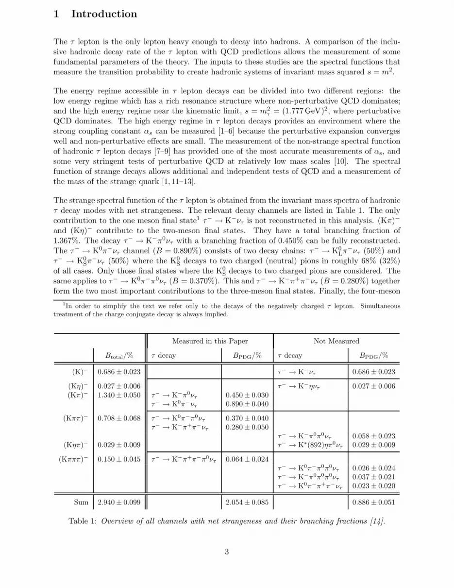
The strange spectral function of the τ lepton is obtained from the invariant mass spectra of hadronicτ decay modes with net strangeness. The relevant decay channels are listed in Table 1. The onlycontribution to the one meson final state1 τ− → K−ντ is not reconstructed in this analysis. (Kπ)−
and (Kη)− contribute to the two-meson final states. They have a total branching fraction of1.367%. The decay τ− → K−π0ντ with a branching fraction of 0.450% can be fully reconstructed.The τ− → K0π−ντ channel (B = 0.890%) consists of two decay chains: τ− → K0
Lπ−ντ (50%) andτ− → K0
Sπ−ντ (50%) where the K0
S decays to two charged (neutral) pions in roughly 68% (32%)of all cases. Only those final states where the K0
S decays to two charged pions are considered. Thesame applies to τ− → K0π−π0ντ (B = 0.370%). This and τ− → K−π+π−ντ (B = 0.280%) togetherform the two most important contributions to the three-meson final states. Finally, the four-meson
1In order to simplify the text we refer only to the decays of the negatively charged τ lepton. Simultaneous
treatment of the charge conjugate decay is always implied.
Measured in this Paper Not Measured
Btotal/% τ decay BPDG/% τ decay BPDG/%
(K)− 0.686± 0.023 τ− → K−ντ 0.686 ± 0.023
(Kη)− 0.027± 0.006 τ− → K−ηντ 0.027 ± 0.006(Kπ)− 1.340± 0.050 τ− → K−π0ντ 0.450± 0.030
τ− → K0π−ντ 0.890± 0.040
(Kππ)− 0.708± 0.068 τ− → K0π−π0ντ 0.370± 0.040τ− → K−π+π−ντ 0.280± 0.050
τ− → K−π0π0ντ 0.058 ± 0.023(Kηπ)− 0.029± 0.009 τ− → K∗(892)ηπ0ντ 0.029 ± 0.009
(Kπππ)− 0.150± 0.045 τ− → K−π+π−π0ντ 0.064± 0.024τ− → K0π−π0π0ντ 0.026 ± 0.024τ− → K−π0π0π0ντ 0.037 ± 0.021τ− → K0π−π+π−ντ 0.023 ± 0.020
Sum 2.940± 0.099 2.054± 0.085 0.886 ± 0.051
Table 1: Overview of all channels with net strangeness and their branching fractions [14].
3
final state (Kπππ)− is detected via the decay τ− → K−π+π−π0ντ . In addition, the decay K−ηπ0ντ
contributes with 0.029%. Hence, 93.4% of all decay channels of the multi-meson final states withopen strangeness, (Kπ)−, (Kππ)− and (Kπππ)−, were measured. This paper describes the selectionof these dominant channels and the measurement of their invariant mass spectra using data collectedwith the OPAL detector during the LEP-I period from 1991 to 1995. The remaining 6.6% and thefinal states including η mesons are taken from Monte Carlo simulation. The spectral function isthen determined from these spectra and the spectral moments are calculated.
From an experimental point of view, one of the key issues of this analysis is the separation ofcharged kaons and pions via the measurement of energy loss in the OPAL jet chamber in thedense environment of multiprong τ lepton decays. Substantial improvements have been achievedcompared to previous publications [15]. In particular, these improvements have made it possibleto obtain a reliable dE/dx measurement in an environment where three tracks are very close toeach other. The reconstruction of neutral pions is based on the study of shower profiles in theelectromagnetic calorimeter. Furthermore the identification and reconstruction of τ lepton decayswith K0
S → π+π− has been achieved with high efficiency and good mass resolution.
The outline of this paper is as follows: Section 2 gives a short description of the OPAL detectorconcentrating on those components which are important for this analysis. In addition, the τ leptonselection and the Monte Carlo samples used are discussed. Section 3 continues with a discussionof the experimental aspects of this work. The selection of the strange hadronic τ lepton decays isdescribed in Section 4. In Section 5, the results for the branching fractions, the strange spectralfunction and the spectral moments are presented together with a discussion of the systematicuncertainties. The results are summarized in Section 6.
2 Detector and Data Samples
2.1 The OPAL Detector
A detailed description of the OPAL detector can be found elsewhere [17]. A short overview isgiven here of those components that are vital for this analysis. Charged particles are tracked inthe central detector, which is enclosed by a solenoidal magnet, providing an axial magnetic fieldof 0.435T. A high-precision silicon micro-vertex detector surrounds the beam pipe. It covers theangular region of | cos θ| ≤ 0.8 and provides tracking information in the r−φ direction2 (and z from1993) [18]. The silicon detector is surrounded by three drift chambers: a high-resolution vertexdetector, a large-volume jet chamber and z-chambers.
The jet chamber measures the momentum and energy loss of charged particles over 98% of thesolid angle. It is subdivided into 24 sectors in r− φ, each containing a radial plane with 159 anodesense wires parallel to the beam pipe. Cathode wire planes form the boundaries between adjacentsectors. The 3D-coordinates of points along the trajectory of a track are determined from the sensewire position, the drift time (r − φ) and a charge division measurement (z) on the sense wire. Thecombined momentum resolution of the OPAL tracking system is σp/p
2 ≈ 1.5 · 10−3 GeV−1. Fromthe total charge on each anode wire, the energy loss dE/dx is calculated and used for particleidentification. This measurement provides a separation between pions and kaons of at least 2σ inthe momentum range relevant for this analysis (3GeV < p < 35GeV).
Outside the solenoid are scintillation counters which measure the time-of-flight from the interaction
2In the OPAL coordinate system the x-axis points to the center of the LEP ring. The z-axis is in the e− beam
direction. The angle θ is defined relative to the z-axis and φ is the azimuthal angle with respect to the x-axis.
4

region and aid in the rejection of cosmic events. Next is the electromagnetic calorimeter (ECAL),which, in the barrel section, is composed of 9440 lead-glass blocks, approximately pointing tothe interaction region, and covering the range | cos θ| < 0.82. Each block has a (10 × 10) cm2
profile with a depth of 24.6 radiation lengths. The resolution of the ECAL in the barrel region,including the effects of the approximately one radiation length of material in front, is σE/E =√
(0.16)2GeV/E + (0.015)2.
The hadron calorimeter (HCAL) is beyond the electromagnetic calorimeter and is instrumentedwith layers of limited streamer tubes in the iron of the solenoid magnet return yoke. The outsideof the hadron calorimeter is surrounded by the muon chamber system, which is composed of fourlayers of drift chambers in the barrel region.
2.2 Selection of τ Lepton Candidates
For the selection of τ lepton candidates, the standard τ selection procedure described in [16]is used. The decay of the Z0 produces a pair of back-to-back highly relativistic τ leptons. Theirdecay products are strongly collimated and well contained within cones of half-angle 35◦. Therefore,each τ decay is treated separately. In order to have a precise and reliable dE/dx measurementand to avoid regions of non-uniform calorimeter response, this analysis is restricted to the region| cos θ| < 0.68. To reject background from hadronic events, exactly two cones are required anda maximum of six good3 tracks in the event is allowed. This background is further reduced byrequiring that the sum of the charges of all tracks in each individual cone is ±1 and the net chargeof the whole event is zero. A total of 162 477 τ cone candidates survive these selection criteria withan estimated non-τ background fraction of 1.5%.
2.3 Simulation of Events
The τ Monte Carlo samples used consist of 200 000 τ pair events generated at√
s = mZ0 usingKORALZ 4.02 [19] and a modified version of TAUOLA 2.4 [20]. Modifications were necessarybecause all four- and five-meson final states with kaons (signal as well as background) are missingin the standard version. Since the resonance structure of these channels is poorly known, onlyphase space distributions of these final states were generated. In addition, the resonance structureof various final states was modified to give a better description of the data [21,22]. The branchingfractions of the decay channels with kaons are enhanced in this sample so that it comprises roughlya factor of ten more τ decays with kaons than expected from data. The Monte Carlo events arethen reweighted to the latest branching fractions given in [14], which are used throughout theselection procedure. The Monte Carlo events were processed through the GEANT OPAL detectorsimulation [23].
The non-τ background was simulated using Monte Carlo samples that consist of 4 000 000 qq eventsgenerated with JETSET [24], 574 000 Bhabha events generated with BHWIDE [25], 792 000 µ-pair events generated with KORALZ [19] and 1 755 000 two-photon events using PHOJET [26],F2GEN [27] and VERMASEREN [28,29].
3A good track has a minimum number of 20 hits in the jet chamber, a maximum |d0| of 2 cm, a maximum |z0|of 75 cm, at least 100 MeV transverse momentum and a maximum radius of the first measured point on the track of
75 cm.
5
3 Identification of Hadrons in τ Final States
3.1 Energy Loss Measurement in τ Decays with Three or More Tracks
A crucial part of this analysis is the identification of charged kaons via energy loss measurement inthe jet chamber. Since this is the only means of distinguishing between charged pions and kaons inOPAL, a very good understanding of the effects present in the multi-track environment in τ leptondecays is vital for any analysis that requires particle identification.
The high Lorentz boost (γ ≈ 25) of the τ lepton results in its decay products being contained ina narrow cone with a typical opening angle of 5◦. In those cases where the final state consists ofmore than one track, the dE/dx measurement is known to be no longer reliable [15]. A systematicshift in the dE/dx distribution is observed which leads to a misidentification of charged pions askaons and thus to a reduced sensitivity in those cases where particle identification is required. Thereason is explained in the following text.
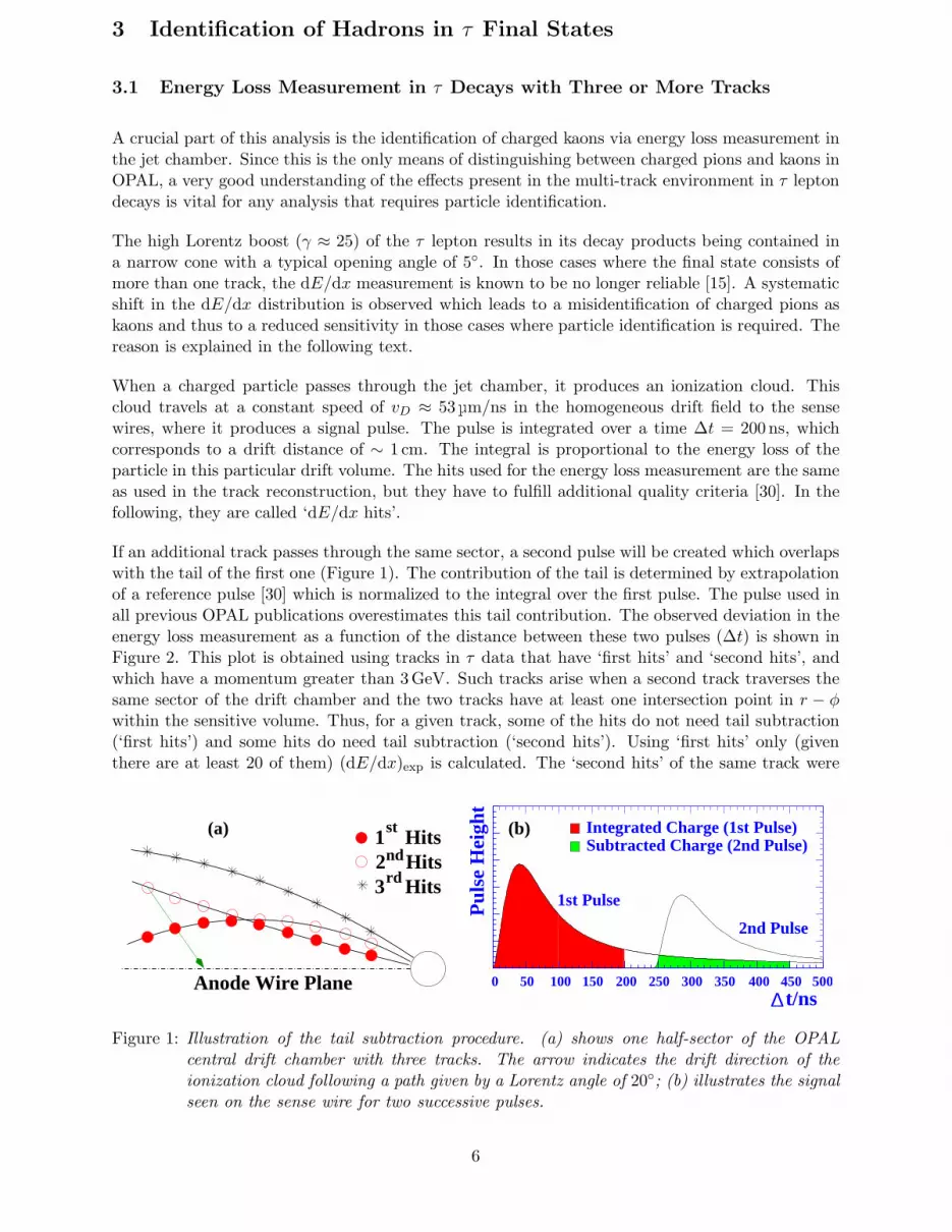
When a charged particle passes through the jet chamber, it produces an ionization cloud. Thiscloud travels at a constant speed of vD ≈ 53µm/ns in the homogeneous drift field to the sensewires, where it produces a signal pulse. The pulse is integrated over a time ∆t = 200ns, whichcorresponds to a drift distance of ∼ 1 cm. The integral is proportional to the energy loss of theparticle in this particular drift volume. The hits used for the energy loss measurement are the sameas used in the track reconstruction, but they have to fulfill additional quality criteria [30]. In thefollowing, they are called ‘dE/dx hits’.
If an additional track passes through the same sector, a second pulse will be created which overlapswith the tail of the first one (Figure 1). The contribution of the tail is determined by extrapolationof a reference pulse [30] which is normalized to the integral over the first pulse. The pulse used inall previous OPAL publications overestimates this tail contribution. The observed deviation in theenergy loss measurement as a function of the distance between these two pulses (∆t) is shown inFigure 2. This plot is obtained using tracks in τ data that have ‘first hits’ and ‘second hits’, andwhich have a momentum greater than 3GeV. Such tracks arise when a second track traverses thesame sector of the drift chamber and the two tracks have at least one intersection point in r − φwithin the sensitive volume. Thus, for a given track, some of the hits do not need tail subtraction(‘first hits’) and some hits do need tail subtraction (‘second hits’). Using ‘first hits’ only (giventhere are at least 20 of them) (dE/dx)exp is calculated. The ‘second hits’ of the same track were
Integrated Charge (1st Pulse)Subtracted Charge (2nd Pulse)
∆ t/ns
Pul
se H
eigh
t
1st Pulse
2nd Pulse
0 50 100 150 200 250 300 350 400 450 500
(a) (b)nd
st
rd2 Hits1 Hits
Anode Wire Plane
3 Hits
Figure 1: Illustration of the tail subtraction procedure. (a) shows one half-sector of the OPALcentral drift chamber with three tracks. The arrow indicates the drift direction of theionization cloud following a path given by a Lorentz angle of 20◦; (b) illustrates the signalseen on the sense wire for two successive pulses.
6
∆
0.80
t/ns
0.90
(dE
/dx)
1.00
mea
s
300
/(dE
/dx)
1000ex
p
4000
OPAL corrected (2nd
OPAL
hits)
Error Band
OPAL corrected (3rd hits) − 0.1
∆t/ns
(dE
/dx)
mea
s / (d
E/d
x)ex
p
0.80
0.90
1.00
300 1000 4000
OPAL
(a) Second Hits
(b) Third Hits
(c)
Error Band
0.80
∆
0.90
t/ns
1.00
(dE
/dx)
mea
s / (d
E/d
x)ex
p
500 1000 1500 2000 2500 3000 3500 4000 4500
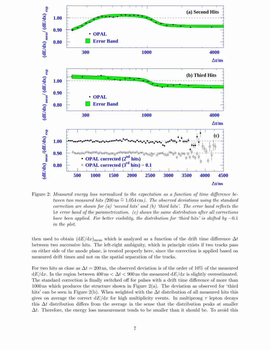
Figure 2: Measured energy loss normalized to the expectation as a function of time difference be-tween two measured hits (200 ns = 1.054 cm). The observed deviations using the standardcorrection are shown for (a) ‘second hits’ and (b) ‘third hits’. The error band reflects the1σ error band of the parametrization. (c) shows the same distribution after all correctionshave been applied. For better visibility, the distribution for ‘third hits’ is shifted by −0.1in the plot.
then used to obtain (dE/dx)meas which is analyzed as a function of the drift time difference ∆tbetween two successive hits. The left-right ambiguity, which in principle exists if two tracks passon either side of the anode plane, is treated properly here, since the correction is applied based onmeasured drift times and not on the spatial separation of the tracks.
For two hits as close as ∆t = 200ns, the observed deviation is of the order of 10% of the measureddE/dx. In the region between 400 ns < ∆t < 900 ns the measured dE/dx is slightly overestimated.The standard correction is finally switched off for pulses with a drift time difference of more than1000 ns which produces the structure shown in Figure 2(a). The deviation as observed for ‘thirdhits’ can be seen in Figure 2(b). When weighted with the ∆t distribution of all measured hits thisgives on average the correct dE/dx for high multiplicity events. In multiprong τ lepton decaysthis ∆t distribution differs from the average in the sense that the distribution peaks at smaller∆t. Therefore, the energy loss measurement tends to be smaller than it should be. To avoid this
7
problem, previous analyses [15] exploited the dE/dx information only of those tracks closest tothe anode plane to classify the τ decay mode. This however significantly reduces the number ofidentified decays.
For this analysis, a new reference pulse has been developed that avoids the shortcomings of thestandard one. In addition, a parametrized pulse shape was used instead of a binned one to avoidartifacts like the dip at ∆t ≈ 500 ns. The new reference pulse is of the form
Pnorm =
(p1∆t exp(−∆t
p2) + p3(∆t)2 exp(−(∆t)2
p4)
)
+
(p5∆t exp(−∆t
p6) + p7(∆t)2 exp(−(∆t)2
p8)
)
+ p1 + p2∆t (1)
with two terms to describe the short-range and the long-range part respectively plus a linearcontribution. The pi are parameters that are optimized for the multi-track environment in τ leptondecays. The correction is applied to all hits. The effect of the correction described above can be seenin Figure 2(c) for ‘second hits’ and ‘third hits’. Apart from this normalization correction, a furtherbias reduction is obtained by also correcting the shape of the reference pulse depending on the chargedeposited by the preceding pulse. In general, the new reference pulse shows a steeper rise at low ∆tand a lower tail to avoid overestimation of the tail subtraction for subsequent pulses as explainedabove. As a result of this procedure, a dE/dx bias reduction to ±1% in (dE/dx)meas/(dE/dx)exp
has been achieved. As the procedure is applied iteratively, i.e. the first pulse is used to correct thesecond, the first and corrected second pulse are used to correct a possible third pulse and so on,the chosen reference pulse is valid for any jet topology [30].
If a track is close to the anode or cathode plane in the jet chamber, the drift field is no longerhomogeneous and one observes a deviation in the measured dE/dx of the order of 3%. Correctionsfor this effect are determined using Z0 → µ−µ+ events.
When a signal is measured at a sense wire, an induced signal at the neighboring wires is also present.This effect depends on the momentum (or curvature) of the track and on cos θ. Corrections havebeen determined using µ-pairs and τ → µνµντ decays. The effect is largest (∼ 5%) for cos θ ∼ 0and large track momenta.
Finally, hits are discarded from tracks where the corresponding hit from the following or thepreceding track is missing. In those cases, the measured dE/dx is overestimated since the chargeis not correctly distributed among the hits but is assigned to one hit only. By discarding this kindof hits, (3 − 5)% of all dE/dx hits are lost.
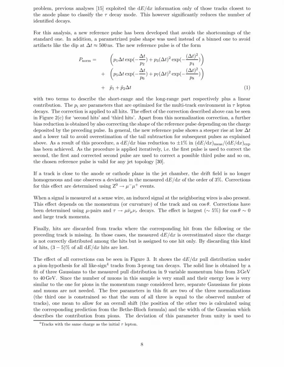
The effect of all corrections can be seen in Figure 3. It shows the dE/dx pull distribution undera pion-hypothesis for all like-sign4 tracks from 3-prong tau decays. The solid line is obtained by afit of three Gaussians to the measured pull distribution in 9 variable momentum bins from 3GeVto 40GeV. Since the number of muons in this sample is very small and their energy loss is verysimilar to the one for pions in the momentum range considered here, separate Gaussians for pionsand muons are not needed. The free parameters in this fit are two of the three normalizations(the third one is constrained so that the sum of all three is equal to the observed number oftracks), one mean to allow for an overall shift (the position of the other two is calculated usingthe corresponding prediction from the Bethe-Bloch formula) and the width of the Gaussian whichdescribes the contribution from pions. The deviation of this parameter from unity is used to
4Tracks with the same charge as the initial τ lepton.
8
Num
ber
of T
rack
s
K e
π/µ
OPAL (corrected)
OPAL (default)
FIT
( dE/dx meas − dE/dxexp )/ σdE/dxexp
10−1
1
10
10 2
10 3
−8 −6 −4 −2 0 2 4 6 8 10
0
2
−8 −6 −4 −2 0 2 4 6 8 10
Figure 3: Pull distribution obtained under a pion hypothesis for all tracks in 3-prong τ lepton decayswith a minimum momentum of 3GeV and a minimum number of 20 hits in the dE/dxmeasurement. Only the tracks with the same charge as the decaying τ lepton are shown.The solid points with error bars are data after all corrections and the function shows theexpectation as explained in the text. The open points in the range between -8 to -2 showthe same distribution but without the corrections mentioned in the text. The smaller plotat the bottom shows the ratio of the full data points to the sum of the functions.
obtain correction factors for the error of the energy loss measurement. The width of the two otherGaussians is calculated assuming that the relative error is constant.
From the measured energy loss, its error and the expectation calculated using the Bethe-Blochequation, χ2 probabilities are calculated that the measured energy deposition is in accordancewith the expectation for a given particle type. Pion- and kaon-weights, Wπ and WK, as used inthis paper, are then calculated by taking one minus the value of this probability. These weightsacquire a sign depending on whether the actual energy loss lies above or below the expectation for acertain particle hypothesis. This means that Wπ is expected to be close to −1 for kaons since theirenergy loss per unit length is smaller in the momentum range relevant in this analysis. For electrontracks, Wπ is expected to be close to +1 due to the higher energy loss in this case. Whenever thesequantities are used in the selection, a cut on at least 20 dE/dx hits for this track is made implicitly.
3.2 Photon Reconstruction and Identification of Neutral Pions
The reconstruction of π0 mesons from photon candidates starts from an algorithm that has beenused in previous OPAL publications (see e.g. [7]). It is based on the analysis of shower profiles inthe ECAL as a function of the energy and direction of photons. In the fit each cluster is treated
9
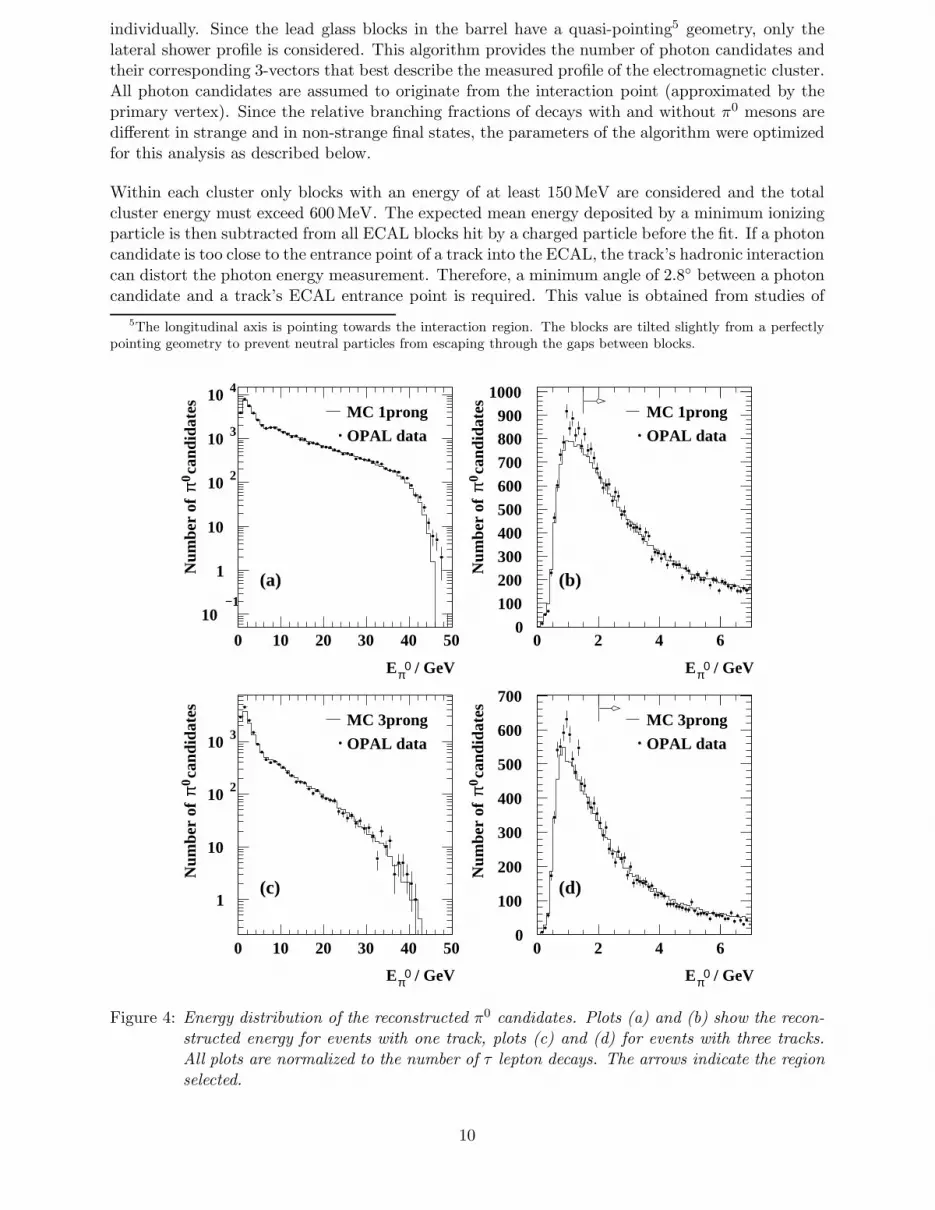
individually. Since the lead glass blocks in the barrel have a quasi-pointing5 geometry, only thelateral shower profile is considered. This algorithm provides the number of photon candidates andtheir corresponding 3-vectors that best describe the measured profile of the electromagnetic cluster.All photon candidates are assumed to originate from the interaction point (approximated by theprimary vertex). Since the relative branching fractions of decays with and without π0 mesons aredifferent in strange and in non-strange final states, the parameters of the algorithm were optimizedfor this analysis as described below.
Within each cluster only blocks with an energy of at least 150MeV are considered and the totalcluster energy must exceed 600MeV. The expected mean energy deposited by a minimum ionizingparticle is then subtracted from all ECAL blocks hit by a charged particle before the fit. If a photoncandidate is too close to the entrance point of a track into the ECAL, the track’s hadronic interactioncan distort the photon energy measurement. Therefore, a minimum angle of 2.8◦ between a photoncandidate and a track’s ECAL entrance point is required. This value is obtained from studies of
5The longitudinal axis is pointing towards the interaction region. The blocks are tilted slightly from a perfectly
pointing geometry to prevent neutral particles from escaping through the gaps between blocks.
Eπ0 / GeV
Num
ber
of
ca
ndid
ates
Num
ber
of
ca
ndid
ates
Num
ber
of
ca
ndid
ates
Num
ber
of
ca
ndid
ates
MC 1prong
OPAL data
(a)
Eπ0 / GeV
MC 1prong
OPAL data
(b)
Eπ0 / GeV
MC 3prong
OPAL data
(c)
Eπ0 / GeV
MC 3prong
OPAL data
(d)
10−1
1
10
10 2
10 3
10 4
0 10 20 30 40 50
ππ π
π
00 0
0
1
10
10 2
10 3
0 10 20 30 40 500
100
200
300
400
500
600
700
0 2 4 6
0
100
200
300
400
500
600
700
800900
1000
0 2 4 6
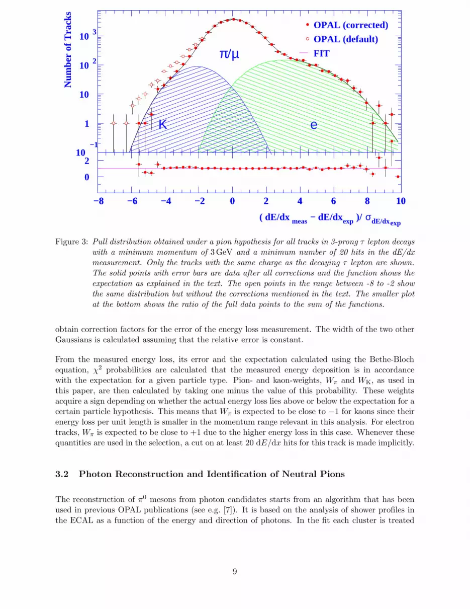
Figure 4: Energy distribution of the reconstructed π0 candidates. Plots (a) and (b) show the recon-structed energy for events with one track, plots (c) and (d) for events with three tracks.All plots are normalized to the number of τ lepton decays. The arrows indicate the regionselected.
10
the rate of fake π0 mesons in the decay τ− → K−ντ and subsequent optimization. To improvethe energy resolution and the purity of the selection, a pairing algorithm is applied to recombinefake photon candidates with the closest photon candidates that were wrongly split up by thereconstruction procedure. The recombination is performed using the Jade jet finding scheme withthe P0 option [31]. Jet resolution parameter ycut values are optimized to obtain the best descriptionof the number of expected photons using Monte Carlo events. Two ycut values are determined, onefor clusters where a track is pointing to one of the blocks in the cluster and one for those withouttracks. This is necessary since the hadronic interaction of charged particles disturbs the showerprofile. The optimized ycut values are −3 and −4.6 for clusters with and without tracks, respectively.The angular resolution of this algorithm is 2.1◦ for clusters with tracks and 1.7◦ for clusters withouttracks. Since these opening angles correspond directly to the energy of the neutral pion, photoncandidates with an energy of more than 7.5GeV are directly interpreted as neutral pion and the4-vector is corrected to account for the π0 mass. The energy of the reconstructed π0 candidates forevents with one and three tracks is shown in Figure 4. The plots are normalized to the number of τdecays in the event sample. Neutral pion candidates with an energy below 1.5GeV in the 1-prongcase and 2GeV in the 3-prong case are rejected.
For the remaining photon candidates, all two-photon combinations are tested. The combinationwhich results in the maximum number of neutral pions with invariant two-photon masses notexceeding the π0 mass by more than 1.5σ is retained. A fit with a π0 mass constraint is then appliedto all π0 candidates. All π0 candidates are assumed to originate from the primary interaction point.
3.3 Identification of K0S
The K0 signal consists of 50% K0L and 50% K0
S. The signature of a K0L decay is a large energy deposit
in the hadron calorimeter without an associated track pointing to the cluster. The resolution of theOPAL hadron calorimeter would not allow for a clean reconstruction of this channel, thus it is notconsidered here. For the K0
S, two decay modes are dominant, K0S → π0π0 (≈ 32%) and K0
S → π+π−
(≈ 68%). In this analysis only the latter is considered since the photon reconstruction algorithmexploits the quasi-pointing geometry of the electromagnetic calorimeter in the barrel (see Section3.2). Thus only photons from the primary vertex can be properly reconstructed.
The selection starts by combining each pair of oppositely charged tracks. Each track must have atransverse momentum with respect to the beam axis of pT ≥ 150MeV, a minimum of 20 out of 159possible hits in CJ, at least 20% of all geometrically possible hits and a maximum χ2 for the trackfit of 50. For each combination of tracks, their intersection points in the plane perpendicular tothe beam axis are calculated. The one with a radius less than 150 cm is selected as the secondaryvertex. If two vertices are found that satisfy this condition, the one with the first measured hitclosest to the intersection point is selected. In addition, the z-coordinate of the vertex has to satisfy|zV| < 80 cm.
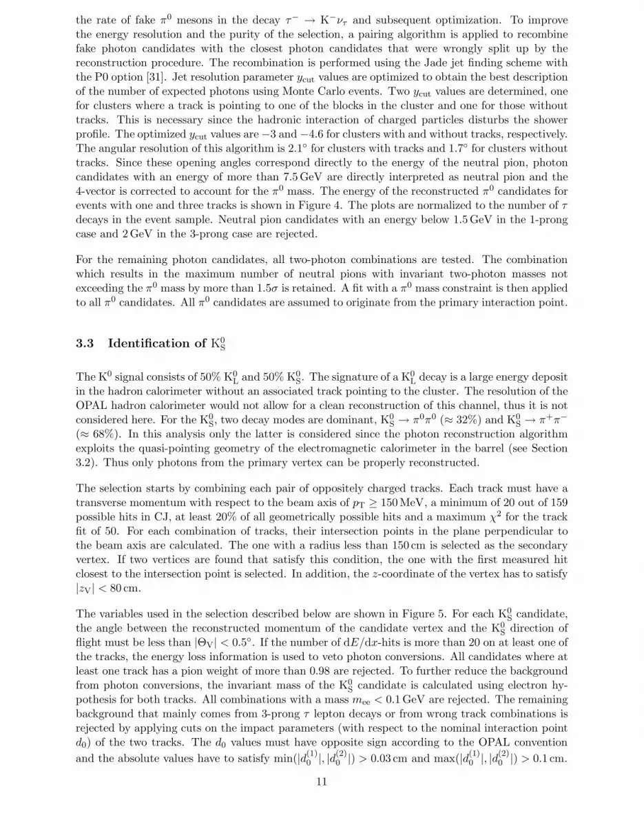
The variables used in the selection described below are shown in Figure 5. For each K0S candidate,
the angle between the reconstructed momentum of the candidate vertex and the K0S direction of
flight must be less than |ΘV| < 0.5◦. If the number of dE/dx-hits is more than 20 on at least one ofthe tracks, the energy loss information is used to veto photon conversions. All candidates where atleast one track has a pion weight of more than 0.98 are rejected. To further reduce the backgroundfrom photon conversions, the invariant mass of the K0
S candidate is calculated using electron hy-pothesis for both tracks. All combinations with a mass mee < 0.1GeV are rejected. The remainingbackground that mainly comes from 3-prong τ lepton decays or from wrong track combinations isrejected by applying cuts on the impact parameters (with respect to the nominal interaction pointd0) of the two tracks. The d0 values must have opposite sign according to the OPAL convention
and the absolute values have to satisfy min(|d(1)0 |, |d(2)
0 |) > 0.03 cm and max(|d(1)0 |, |d(2)
0 |) > 0.1 cm.
11
mee/GeV
(a)
|ΘV|/degree
(b)
min(|d0(1)|,|d0
(2)|)/cm
(c)
max(|d0(1)|,|d0
(2)|)/cm
(d)
π-Weight
(e)OPALK0
SBackgroundPhoton Conversions
0
50
100
150
200
250
0 0.2 0.4 0.6 0.8 10
100
200
300
0 0.2 0.4 0.6 0.8 1
0
200
400
600
0 0.05 0.1 0.15 0.2 0.25 0.30
50
100
150
200
250
0 0.05 0.1 0.15 0.2 0.25 0.3
10
10 2
10 3
-1 -0.8 -0.6 -0.4 -0.2 0 0.2 0.4 0.6 0.8 1
S0K
Num
ber
of
C
andi
date
sS0
KN
umbe
r of
Can
dida
tes
S0K
Num
ber
of
C
andi
date
sS0
KN
umbe
r of
Can
dida
tes
S0K
Num
ber
of
C
andi
date
s
Figure 5: Variables used in the K0S selection. A detailed description of all variables is given in the
text. The dots represent the data and the open histogram is Monte Carlo signal. Theshaded areas show the background where photon conversions are marked separately. Thearrows indicate the region selected. For all plots, all selection cuts have been appliedexcept for the cut on the variable shown. All plots are normalized to the number of τdecays.
12
mππ/GeV
(a)
Radius(Sec. Vertex)/cm
(b)
χ2 Probability
OPALK0
S
BackgroundPhoton Conversions
(c)
0
50
100
150
200
250
300
0.2 0.4 0.6 0.8 1 1.20
20406080
100120140160180200
0 50 100 150
1
10
10 2
0 0.1 0.2 0.3 0.4 0.5 0.6 0.7 0.8 0.9 1
KS0
Num
ber
of
C
andi
date
s
KS0
Num
ber
of
C
andi
date
s
KS0
Num
ber
of
C
andi
date
s
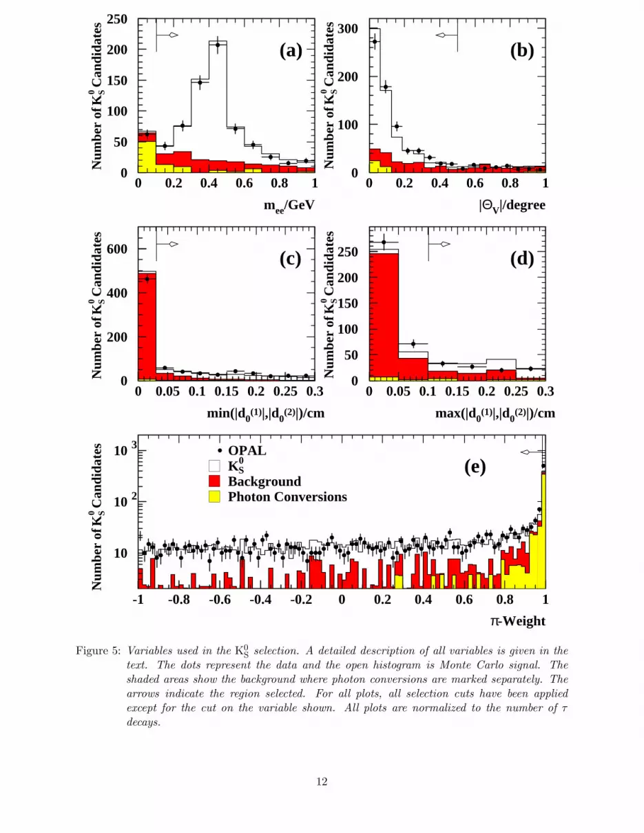
Figure 6: Result of the K0S selection. Plot (a) shows the invariant mass distribution of the K0
S
candidates under pion hypothesis before the kinematic fit. Plot (b) shows the radius ofthe reconstructed secondary vertex and plot (c) the distribution of the χ2-probability ofthe 2C-fit. A cut is applied on the probability at 10−5. The dots represent the data andthe open histogram is the Monte Carlo signal. The shaded areas show the backgroundwhere photon conversions are marked separately. All plots are normalized to the numberof τ decays.
The remaining K0S candidates must have a momentum of pK0
S
> 3GeV. A 3D vertex fit is applied toeach candidate, that includes a constraint of the invariant two-track mass under the pion hypothesisto the nominal K0
S mass. This is a 2C fit and a cut on the χ2 probability at 10−5 is applied.The invariant two-track mass under the pion hypothesis before the kinematic fit can be found inFigure 6 together with the radius of the reconstructed secondary vertex and the χ2 probabilityof the kinematic fit. In Figure 6(a) the ππ-invariant mass spectrum is shown without any vertexconstraint. If more than one K0
S candidate shares the same track, the one with the smallest deviationfrom the nominal K0
S mass before the fit is selected.
After this selection procedure, a total of 535 K0S candidates remain with an estimated purity of
82%. About 70% of the background consists of wrong combinations of tracks, and 30% comes fromphoton conversions. In one data event, two K0
S candidates are found within one cone. This eventis considered to be background.
13
4 Identification of τ Final States
For the selection of the various final states, a cut-based procedure is used where each τ decay istreated independently. For all selected decay modes, the cone axis, calculated from the momentaof all tracks and neutral clusters identified in the electromagnetic calorimeter, must have a polarangle within | cos θ| < 0.68 for the reasons explained above. Each selected cone must have at leastone good track coming from the interaction point and the summed momenta of all tracks have tobe less than the beam energy. Since there is at least one hadron in the final states considered here,the total energy deposited in the hadron calorimeter within the cone is required to exceed 1GeV.
4.1 Corrections to the Invariant Mass Spectra
The spectral function from τ lepton decays is a weighted invariant mass distribution of all hadronicfinal states with strangeness. The various final states have different experimental resolutions andmigration effects that must be corrected for. To correct the observed data, the following methodwas used. The elements cij of the inverse detector response matrix were determined directly fromMonte Carlo. They represent the probability that an event reconstructed in bin j was generatedin bin i. To calculate this probability Monte Carlo samples for the signal channels with massdistributions according to phase space were used. The corrected distribution was then obtained by
gCorrectedi =
∑
j
cij(gDATAj − gBackground
j ) (2)
where gDATAj is the number of events in the data with a reconstructed mass in bin j, gBackground
j
is the number of background events predicted in bin j and gCorrectedi the number of events in mass
bin i after correction.
The corrected distributions will in general be biased towards the Monte Carlo input distributions.To reduce the bias from this approach, the method was applied iteratively. The result of thepreceding iteration was used to refine the elements of the inverse detector matrix. The optimalnumber of iterations was determined, using Monte Carlo simulations, to be two for all final statesconsidered here. The corresponding systematic uncertainties are discussed in Section 5.4. Finally,detection efficiency corrections were applied to the corrected invariant mass distributions. Thebin width of 150MeV of the measured invariant mass spectra were chosen according to the massresolution of the τ decay channels measured.
4.2 (Kπ)− Final States
The (Kπ)− mass spectrum consists of two measured modes, K−π0ντ and K0π−ντ . From the latterdecay mode, only the decays K0
S → π+π− are measured. The K∗(892) dominance is well establishedin both cases.
4.2.1 K−π0ντ
In the K−π0ντ selection, exactly one good track coming from the primary vertex is required. Thistrack must have a minimum momentum of p > 3GeV. For the track to be selected as a kaon, thepion weight has to satisfy Wπ < −0.98 and the kaon weight WK < 0.6. Furthermore, exactly one
14
identified neutral pion is required with Eπ0
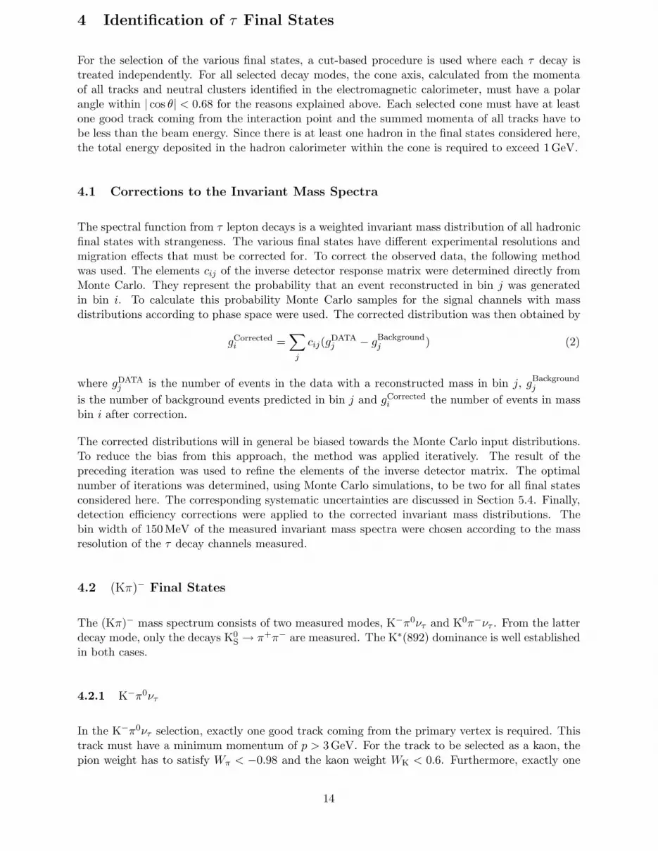
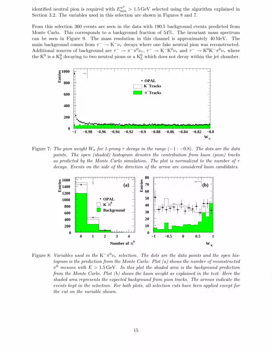
min > 1.5GeV selected using the algorithm explained inSection 3.2. The variables used in this selection are shown in Figures 8 and 7.
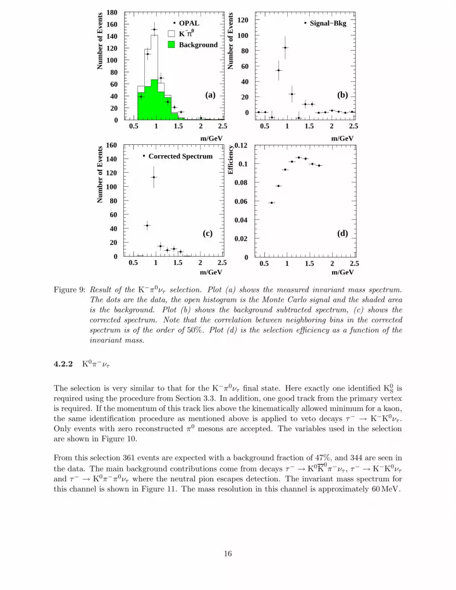
From this selection 360 events are seen in the data with 190.5 background events predicted fromMonte Carlo. This corresponds to a background fraction of 54%. The invariant mass spectrumcan be seen in Figure 9. The mass resolution in this channel is approximately 40MeV. Themain background comes from τ− → K−ντ decays where one fake neutral pion was reconstructed.Additional sources of background are τ− → π−π0ντ , τ− → K−K0ντ and τ− → K0K−π0ντ wherethe K0 is a K0
S decaying to two neutral pions or a K0L which does not decay within the jet chamber.
Wπ
Ent
ries
OPAL
π
K−
−
Tracks
Tracks
0
200
400
600
800
1000
−1 −0.98 −0.96 −0.94 −0.92 −0.9 −0.88 −0.86 −0.84 −0.82 −0.8
Figure 7: The pion weight Wπ for 1-prong τ decays in the range (−1 : −0.8). The dots are the datapoints. The open (shaded) histogram denotes the contribution from kaon (pion) tracksas predicted by the Monte Carlo simulation. The plot is normalized to the number of τdecays. Events on the side of the direction of the arrow are considered kaon candidates.
Number of π0
Ent
ries
OPALK −π0
Background
W K
Ent
ries
0
200
400
600
800
1000
1200
1400
1600
0 1 2 3 40
10
20
30
40
50
60
70
80
−1 −0.5 0 0.5 1
(a) (b)
Figure 8: Variables used in the K−π0ντ selection. The dots are the data points and the open his-togram is the prediction from the Monte Carlo. Plot (a) shows the number of reconstructedπ0 mesons with E > 1.5GeV. In this plot the shaded area is the background predictionfrom the Monte Carlo. Plot (b) shows the kaon weight as explained in the text. Here theshaded area represents the expected background from pion tracks. The arrows indicate theevents kept in the selection. For both plots, all selection cuts have been applied except forthe cut on the variable shown.
15
m/GeV m/GeV
m/GeV
Eff
icie
ncy
Num
ber
of E
vent
sN
umbe
r of
Eve
nts
OPAL
Corrected Spectrum
K−π0
Background
m/GeV
Num
ber
of E
vent
s
Signal−Bkg
0
0.02
0
0.04
20
0.06
40
0.08
60
0.1
80
0.12
100
0
120
20
140
40
160
60
180
80
100
120
140
160
0.5 1 1.5 2 2.5
0.5 1 1.5 2 2.5
0.5 1 1.5 2 2.5
0
20
40
60
80
100
120
0.5 1 1.5 2 2.5
(b)(a)
(d)(c)
Figure 9: Result of the K−π0ντ selection. Plot (a) shows the measured invariant mass spectrum.The dots are the data, the open histogram is the Monte Carlo signal and the shaded areais the background. Plot (b) shows the background subtracted spectrum, (c) shows thecorrected spectrum. Note that the correlation between neighboring bins in the correctedspectrum is of the order of 50%. Plot (d) is the selection efficiency as a function of theinvariant mass.
4.2.2 K0π−ντ
The selection is very similar to that for the K−π0ντ final state. Here exactly one identified K0S is
required using the procedure from Section 3.3. In addition, one good track from the primary vertexis required. If the momentum of this track lies above the kinematically allowed minimum for a kaon,the same identification procedure as mentioned above is applied to veto decays τ− → K−K0ντ .Only events with zero reconstructed π0 mesons are accepted. The variables used in the selectionare shown in Figure 10.
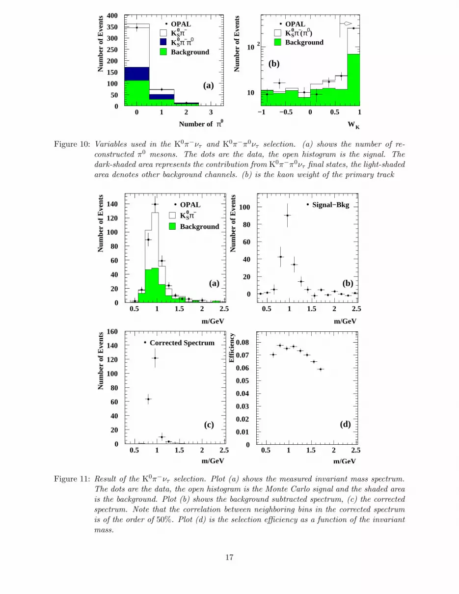
From this selection 361 events are expected with a background fraction of 47%, and 344 are seen in
the data. The main background contributions come from decays τ− → K0K0π−ντ , τ− → K−K0ντ
and τ− → K0π−π0ντ where the neutral pion escapes detection. The invariant mass spectrum forthis channel is shown in Figure 11. The mass resolution in this channel is approximately 60MeV.
16
WK
Num
ber
of E
vent
s
OPALOPALK
KK 0
0
0S
S
S πππ −
−
− (ππ
0
0)
BackgroundBackground
Number of π0
Num
ber
of E
vent
s10
10 2
−1 −0.5 0 0.5 10
50
100
150
200
250
300
350
400
0 1 2 3
(a)
(b)
Figure 10: Variables used in the K0π−ντ and K0π−π0ντ selection. (a) shows the number of re-constructed π0 mesons. The dots are the data, the open histogram is the signal. Thedark-shaded area represents the contribution from K0π−π0ντ final states, the light-shadedarea denotes other background channels. (b) is the kaon weight of the primary track
m/GeV
m/GeV
Num
ber
of E
vent
sN
umbe
r of
Eve
nts
OPAL
Corrected Spectrum
K0Sπ−
Background
m/GeV
Num
ber
of E
vent
s
Signal−Bkg
0
20
40
60
80
100
120
140
160
0.5 1 1.5 2 2.5
0
20
40
60
80
100
120
140
0.5 1 1.5 2 2.5
(b)(a)
(d)(c)
0
20
40
60
80
100
0.5 1 1.5 2 2.5
Effi
cien
cy
0
0.01
0.02
0.03
0.04
0.05
0.06
0.07
0.08
0.5 1 1.5 2 2.5
m/GeV
Figure 11: Result of the K0π−ντ selection. Plot (a) shows the measured invariant mass spectrum.The dots are the data, the open histogram is the Monte Carlo signal and the shaded areais the background. Plot (b) shows the background subtracted spectrum, (c) the correctedspectrum. Note that the correlation between neighboring bins in the corrected spectrumis of the order of 50%. Plot (d) is the selection efficiency as a function of the invariantmass.
17
4.3 (Kππ)− Final States
The (Kππ)− final state consists of the decay modes: K−π+π−ντ , K0π−π0ντ and K−π0π0ντ . Toselect these final states, the following procedure is applied.
4.3.1 K−π+π−ντ
The selection starts by requiring exactly three good tracks coming from the interaction point. Thesetracks are fitted to a common vertex and the fit probability is required to be larger than 10−7. Inaddition, each pair of oppositely charged tracks has to fail the selection criteria for neutral kaonsas defined in Section 3.3. These two requirements reduce the background from photon conversionsand decays containing K0
S.
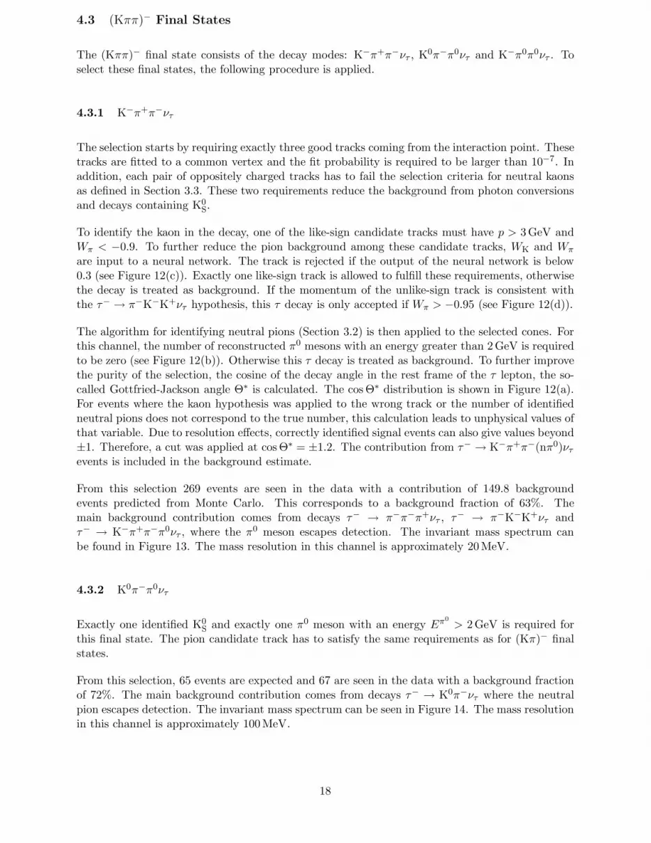
To identify the kaon in the decay, one of the like-sign candidate tracks must have p > 3GeV andWπ < −0.9. To further reduce the pion background among these candidate tracks, WK and Wπ
are input to a neural network. The track is rejected if the output of the neural network is below0.3 (see Figure 12(c)). Exactly one like-sign track is allowed to fulfill these requirements, otherwisethe decay is treated as background. If the momentum of the unlike-sign track is consistent withthe τ− → π−K−K+ντ hypothesis, this τ decay is only accepted if Wπ > −0.95 (see Figure 12(d)).
The algorithm for identifying neutral pions (Section 3.2) is then applied to the selected cones. Forthis channel, the number of reconstructed π0 mesons with an energy greater than 2GeV is requiredto be zero (see Figure 12(b)). Otherwise this τ decay is treated as background. To further improvethe purity of the selection, the cosine of the decay angle in the rest frame of the τ lepton, the so-called Gottfried-Jackson angle Θ∗ is calculated. The cos Θ∗ distribution is shown in Figure 12(a).For events where the kaon hypothesis was applied to the wrong track or the number of identifiedneutral pions does not correspond to the true number, this calculation leads to unphysical values ofthat variable. Due to resolution effects, correctly identified signal events can also give values beyond±1. Therefore, a cut was applied at cos Θ∗ = ±1.2. The contribution from τ− → K−π+π−(nπ0)ντ
events is included in the background estimate.
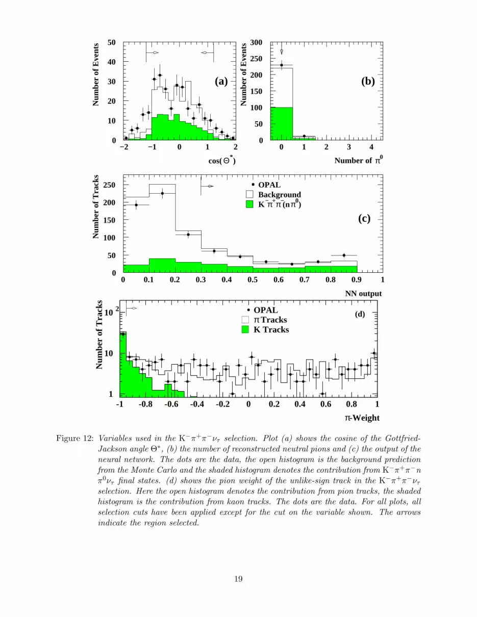
From this selection 269 events are seen in the data with a contribution of 149.8 backgroundevents predicted from Monte Carlo. This corresponds to a background fraction of 63%. Themain background contribution comes from decays τ− → π−π−π+ντ , τ− → π−K−K+ντ andτ− → K−π+π−π0ντ , where the π0 meson escapes detection. The invariant mass spectrum canbe found in Figure 13. The mass resolution in this channel is approximately 20MeV.
4.3.2 K0π−π0ντ
Exactly one identified K0S and exactly one π0 meson with an energy Eπ0
> 2GeV is required forthis final state. The pion candidate track has to satisfy the same requirements as for (Kπ)− finalstates.
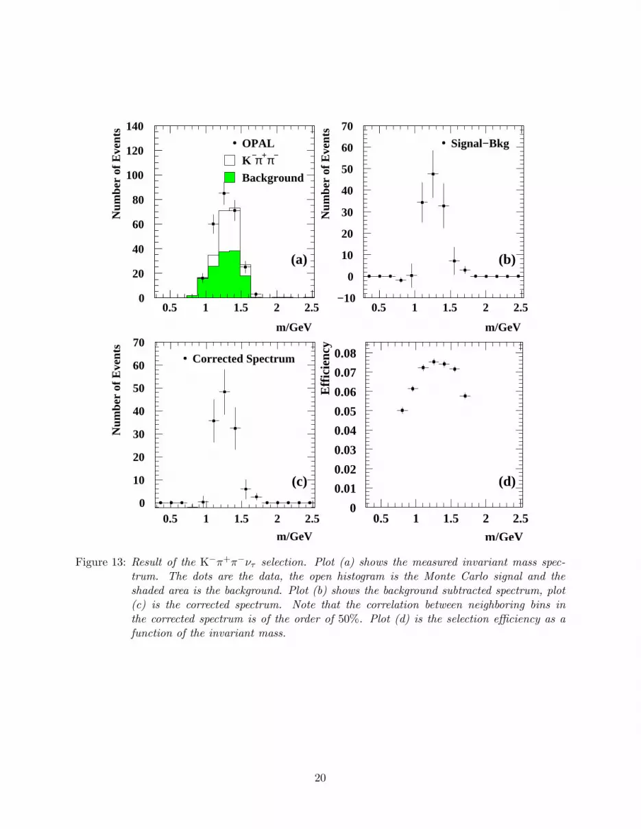
From this selection, 65 events are expected and 67 are seen in the data with a background fractionof 72%. The main background contribution comes from decays τ− → K0π−ντ where the neutralpion escapes detection. The invariant mass spectrum can be seen in Figure 14. The mass resolutionin this channel is approximately 100MeV.
18
cos( Θ*)
Num
ber
of E
vent
s
Number of π0
Num
ber
of E
vent
s
NN output
Num
ber
of T
rack
s
OPALBackgroundK−π+π−(nπ0)
0
10
20
30
40
50
−2 −1 0 1 20
50
100
150
200
250
300
0 1 2 3 4
(a) (b)
(c)
0
50
100
150
200
250
0 0.1 0.2 0.3 0.4 0.5 0.6 0.7 0.8 0.9 1
π-Weight
Num
ber
of T
rack
s
OPALπ TracksK Tracks
1
10
10 2
-1 -0.8 -0.6 -0.4 -0.2 0 0.2 0.4 0.6 0.8 1
(d)
Figure 12: Variables used in the K−π+π−ντ selection. Plot (a) shows the cosine of the Gottfried-Jackson angle Θ∗, (b) the number of reconstructed neutral pions and (c) the output of theneural network. The dots are the data, the open histogram is the background predictionfrom the Monte Carlo and the shaded histogram denotes the contribution from K−π+π−nπ0ντ final states. (d) shows the pion weight of the unlike-sign track in the K−π+π−ντ
selection. Here the open histogram denotes the contribution from pion tracks, the shadedhistogram is the contribution from kaon tracks. The dots are the data. For all plots, allselection cuts have been applied except for the cut on the variable shown. The arrowsindicate the region selected.
19
m/GeV
m/GeV
Num
ber
of E
vent
sN
umbe
r of
Eve
nts
OPAL
Corrected Spectrum
K−π+π−
Background
m/GeVN
umbe
r of
Eve
nts
Signal−Bkg
0
20
40
60
80
100
120
140
0
10
20
30
40
50
0.5
60
1
70
1.5 2 2.5
0.5 1 1.5 2 2.5
−10
0
10
20
30
40
50
60
70
0.5 1 1.5 2 2.5
(a)
(c)
(b)
(d)
0.5 1 1.5 2 2.5
m/GeV
Effi
cien
cy
0
0.01
0.02
0.03
0.04
0.05
0.06
0.07
0.08
Figure 13: Result of the K−π+π−ντ selection. Plot (a) shows the measured invariant mass spec-trum. The dots are the data, the open histogram is the Monte Carlo signal and theshaded area is the background. Plot (b) shows the background subtracted spectrum, plot(c) is the corrected spectrum. Note that the correlation between neighboring bins inthe corrected spectrum is of the order of 50%. Plot (d) is the selection efficiency as afunction of the invariant mass.
20
m/GeV
Num
ber
of E
vent
s
OPAL
K0π−π0
Background
m/GeVN
umbe
r of
Eve
nts
Signal−Bkg
Corrected Spectrum
0
5
10
15
20
25
30
35
40
0.5 1 1.5 2 2.5−4−2024
(a) (b)
(c) (d)
68
101214161820
0.5 1 1.5 2 2.5
m/GeV
0
1
2
3
4
5
6
7
8
9
0.5 1 1.5 2 2.5m/GeV
0
0.005
0.01
0.015
0.02
0.025
0.03
0.035
0.04
0.5 1 1.5 2 2.5
Effi
cien
cy
Num
ber
of E
vent
s
Figure 14: Result of the K0π−π0ντ selection. Plot (a) shows the measured invariant mass spectrum.The dots are the data, the open histogram is the Monte Carlo signal and the shaded areais the background. Plot (b) shows the background subtracted spectrum, (c) the correctedspectrum. Note that the correlation between neighboring bins in the corrected spectrumis of the order of 50%. Plot (d) is the selection efficiency as a function of the invariantmass.
21

4.4 (Kπππ)− Final States
The (Kπππ)− signal consists of the following final states: K−π+π−π0ντ , K0π−π0π0ντ , K−π0π0π0ντ
and K0π−π+π−ντ . From these, only the first one which has the highest branching fraction isinvestigated.
m/GeV
Num
ber
of E
vent
sOPAL
K−π−π+π0
Background
m/GeV
Num
ber
of E
vent
s
Signal−Bkg
0
2
4
6
8
10
12
14
16
18
20
0.5 1 1.5 2 2.5−1012345678
(a) (b)
910
0.5 1 1.5 2 2.5
Figure 15: Result of the K−π+π−π0ντ selection. Plot (a) shows the measured invariant mass spec-trum. The dots are the data, the open histogram is the Monte Carlo signal and theshaded area is the background. Plot (b) shows the background subtracted spectrum.
The same procedure as for the K−π+π−ντ channel is used. In addition, one identified π0 mesonwith an energy of more than 2GeV is required. The invariant mass spectrum can be seen in Figure15. The mass resolution in this channel is approximately 60MeV. From this selection, 14 eventsare seen in the data with a contribution of 10 events from background. The selection efficiency is ofthe order of 1%. The main background contribution comes from τ− → K−π+π−ντ decays, whereone fake neutral pion was identified.
Since the number of signal events in this final state is not significantly different from zero, thischannel is not considered any further in this analysis. For the spectral function, the Monte Carloprediction has been used instead.
5 Results
5.1 Branching Fractions
The measured data used in the spectral function analysis allows the determination of competitivebranching fractions for the channels τ− → K−π0ντ and τ− → K−π+π−ντ . The branching fractionsare determined in a simultaneous χ2 fit, taking all measured final states into account. The fitfunction is
Ni = Nnon−τi + (1 − fnon−τ
bkg ) · N τ∑
j
εijBjFBiasj ,
where i is the signal channel under consideration and index j runs over all τ decay channels. Ni
is the number of decays observed in the data, i.e. the number of τ cones passing the cuts. The
22
number of decays from the non-τ background is denoted by Nnon−τi , fnon−τ
bkg is the fraction of non-
τ background, N τ is the number of τ events, εij the efficiency matrix, FBiasj the bias factor for
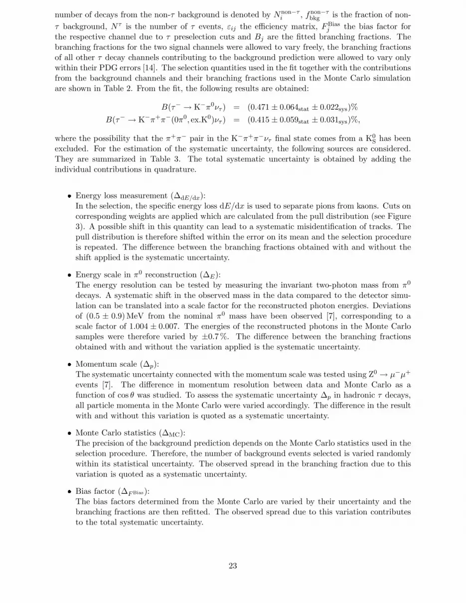
the respective channel due to τ preselection cuts and Bj are the fitted branching fractions. Thebranching fractions for the two signal channels were allowed to vary freely, the branching fractionsof all other τ decay channels contributing to the background prediction were allowed to vary onlywithin their PDG errors [14]. The selection quantities used in the fit together with the contributionsfrom the background channels and their branching fractions used in the Monte Carlo simulationare shown in Table 2. From the fit, the following results are obtained:
B(τ− → K−π0ντ ) = (0.471 ± 0.064stat ± 0.022sys)%
B(τ− → K−π+π−(0π0, ex.K0)ντ ) = (0.415 ± 0.059stat ± 0.031sys)%,
where the possibility that the π+π− pair in the K−π+π−ντ final state comes from a K0S has been
excluded. For the estimation of the systematic uncertainty, the following sources are considered.They are summarized in Table 3. The total systematic uncertainty is obtained by adding theindividual contributions in quadrature.� Energy loss measurement (∆dE/dx):
In the selection, the specific energy loss dE/dx is used to separate pions from kaons. Cuts oncorresponding weights are applied which are calculated from the pull distribution (see Figure3). A possible shift in this quantity can lead to a systematic misidentification of tracks. Thepull distribution is therefore shifted within the error on its mean and the selection procedureis repeated. The difference between the branching fractions obtained with and without theshift applied is the systematic uncertainty.� Energy scale in π0 reconstruction (∆E):The energy resolution can be tested by measuring the invariant two-photon mass from π0
decays. A systematic shift in the observed mass in the data compared to the detector simu-lation can be translated into a scale factor for the reconstructed photon energies. Deviationsof (0.5 ± 0.9)MeV from the nominal π0 mass have been observed [7], corresponding to ascale factor of 1.004 ± 0.007. The energies of the reconstructed photons in the Monte Carlosamples were therefore varied by ±0.7%. The difference between the branching fractionsobtained with and without the variation applied is the systematic uncertainty.� Momentum scale (∆p):The systematic uncertainty connected with the momentum scale was tested using Z0 → µ−µ+
events [7]. The difference in momentum resolution between data and Monte Carlo as afunction of cos θ was studied. To assess the systematic uncertainty ∆p in hadronic τ decays,all particle momenta in the Monte Carlo were varied accordingly. The difference in the resultwith and without this variation is quoted as a systematic uncertainty.� Monte Carlo statistics (∆MC):The precision of the background prediction depends on the Monte Carlo statistics used in theselection procedure. Therefore, the number of background events selected is varied randomlywithin its statistical uncertainty. The observed spread in the branching fraction due to thisvariation is quoted as a systematic uncertainty.� Bias factor (∆FBias):The bias factors determined from the Monte Carlo are varied by their uncertainty and thebranching fractions are then refitted. The observed spread due to this variation contributesto the total systematic uncertainty.
23
τ− → K−π0ντ
No. of Events 360Selection Efficiency /% 8.42 ± 0.17Preselection Bias Factor 1.016 ± 0.011Non-τ Background Fraction 0.006 ± 0.004τ Background Fraction 0.540 ± 0.027
π−π0ντ 13.5% 0.051 ± 0.005 25.41 ± 0.14K−K0π0ντ 9.9% 6.0 ± 0.3 0.155 ± 0.020
K−ντ 8.1% 1.25 ± 0.06 0.686 ± 0.023K−K0ντ 7.3% 4.5 ± 0.2 0.154 ± 0.016
π−π0π0ντ 6.2% 0.07 ± 0.01 9.17 ± 0.14K−π0π0ντ 5.0% 9.6 ± 0.5 0.058 ± 0.023
K−π0π0π0ντ 2.6% 8.9 ± 0.6 0.037 ± 0.021other 1.4%
Bkg. Fraction Efficiency /% BPDG/%
τ− → K−π+π−ντ
No. of Events 269Selection Efficiency/% 6.59 ± 0.06Preselection Bias Factor 0.953 ± 0.013Non-τ Background Fraction 0.007 ± 0.006τ Background Fraction 0.631 ± 0.044
π−π+π−ντ 21.6% 0.15 ± 0.02 9.22 ± 0.10π−K−K+ντ 10.3% 3.9 ± 0.2 0.161 ± 0.019
π−π+π−π0ντ 8.1% 0.5 ± 0.1 4.24 ± 0.10K−π+π−π0ντ 6.7% 2.7 ± 0.2 0.064 ± 0.024
other 16.4%
Bkg. Fraction Efficiency /% BPDG/%
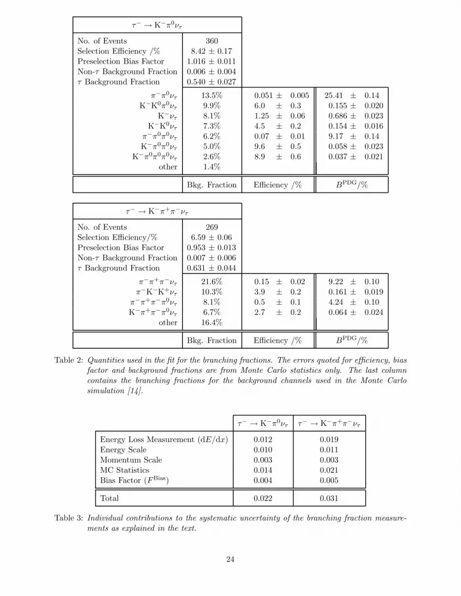
Table 2: Quantities used in the fit for the branching fractions. The errors quoted for efficiency, biasfactor and background fractions are from Monte Carlo statistics only. The last columncontains the branching fractions for the background channels used in the Monte Carlosimulation [14].
τ− → K−π0ντ τ− → K−π+π−ντ
Energy Loss Measurement (dE/dx) 0.012 0.019Energy Scale 0.010 0.011Momentum Scale 0.003 0.003MC Statistics 0.014 0.021Bias Factor (FBias) 0.004 0.005
Total 0.022 0.031
Table 3: Individual contributions to the systematic uncertainty of the branching fraction measure-ments as explained in the text.
24
5.2 Improved Averages for B(τ− → K−π
0ντ ) and B(τ− → K−
π+π−ντ )
For the determination of the spectral function and its moments described below, new average valuesfor the branching fractions of the decays τ− → K−π0ντ and τ− → K−π+π−ντ are determined. Inaddition to the results obtained here, the same measurements are used as inputs for the calculationas in [14]. For the channel τ− → K−π+π−ντ , the previous result from OPAL [32] was replaced bythe measurement obtained in this analysis. Also, the CLEO result was updated using [33]. Thenew averages are:
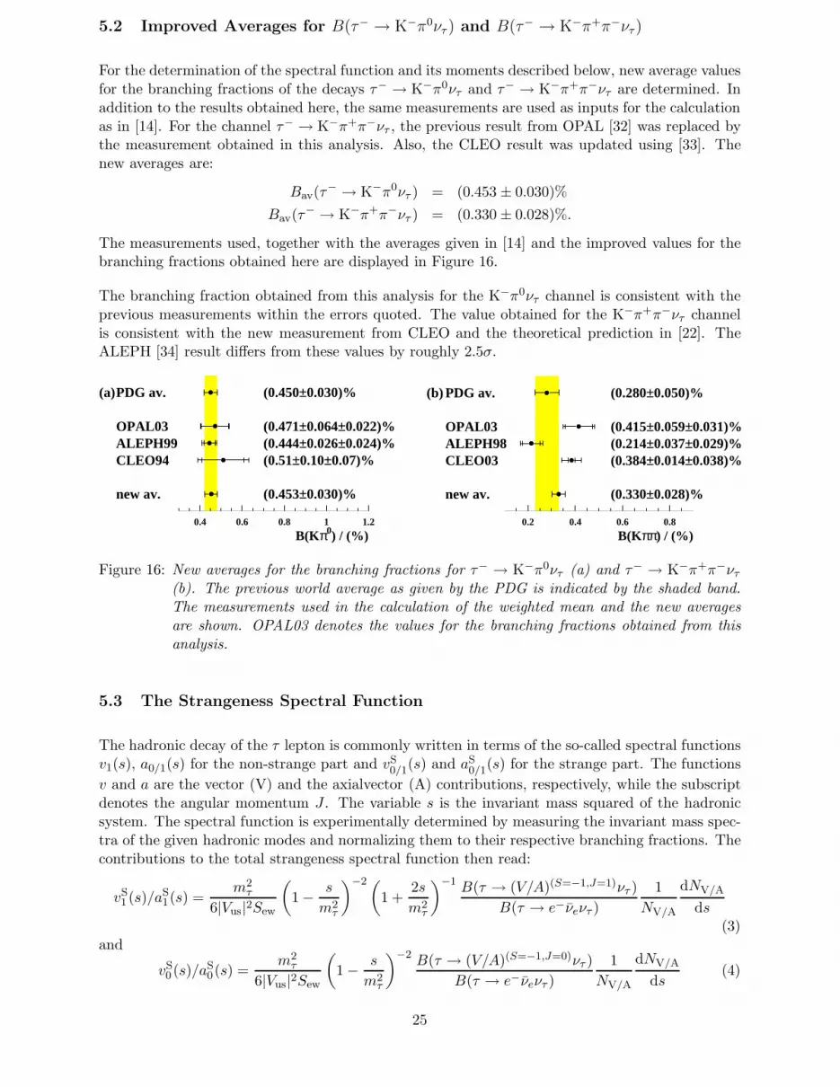
Bav(τ− → K−π0ντ ) = (0.453 ± 0.030)%
Bav(τ− → K−π+π−ντ ) = (0.330 ± 0.028)%.
The measurements used, together with the averages given in [14] and the improved values for thebranching fractions obtained here are displayed in Figure 16.
The branching fraction obtained from this analysis for the K−π0ντ channel is consistent with theprevious measurements within the errors quoted. The value obtained for the K−π+π−ντ channelis consistent with the new measurement from CLEO and the theoretical prediction in [22]. TheALEPH [34] result differs from these values by roughly 2.5σ.
(a)PDG av. (0.450±0.030)%
OPAL03 (0.471±0.064±0.022)%ALEPH99 (0.444±0.026±0.024)%CLEO94 (0.51±0.10±0.07)%
new av. (0.453±0.030)%
B(Kπ0) / (%)0.4 0.6 0.8 1 1.2
(b) PDG av. (0.280±0.050)%
OPAL03 (0.415±0.059±0.031)%ALEPH98 (0.214±0.037±0.029)%CLEO03 (0.384±0.014±0.038)%
new av. (0.330±0.028)%
B(Kππ) / (%)0.2 0.4 0.6 0.8
Figure 16: New averages for the branching fractions for τ− → K−π0ντ (a) and τ− → K−π+π−ντ
(b). The previous world average as given by the PDG is indicated by the shaded band.The measurements used in the calculation of the weighted mean and the new averagesare shown. OPAL03 denotes the values for the branching fractions obtained from thisanalysis.
5.3 The Strangeness Spectral Function
The hadronic decay of the τ lepton is commonly written in terms of the so-called spectral functionsv1(s), a0/1(s) for the non-strange part and vS
0/1(s) and aS0/1(s) for the strange part. The functions
v and a are the vector (V) and the axialvector (A) contributions, respectively, while the subscriptdenotes the angular momentum J . The variable s is the invariant mass squared of the hadronicsystem. The spectral function is experimentally determined by measuring the invariant mass spec-tra of the given hadronic modes and normalizing them to their respective branching fractions. Thecontributions to the total strangeness spectral function then read:
vS1 (s)/aS
1(s) =m2
τ
6|Vus|2Sew
(1 − s
m2τ
)−2 (
1 +2s
m2τ
)−1 B(τ → (V/A)(S=−1,J=1)ντ )
B(τ → e−νeντ )
1
NV/A
dNV/A
ds(3)
and
vS0 (s)/aS
0(s) =m2
τ
6|Vus|2Sew
(1 − s
m2τ
)−2 B(τ → (V/A)(S=−1,J=0)ντ )
B(τ → e−νeντ )
1
NV/A
dNV/A
ds(4)
25
where |Vus| = 0.2196±0.0023 [14] is the CKM weak mixing matrix element, mτ = (1 776.9+0.31−0.27)MeV
[35] and Sew = 1.0194 ± 0.0040 [36] is an electroweak correction factor. The total strangenessspectral function (v + a) is then obtained by adding the individual contributions. To disentanglethe vector and the axialvector contributions for the spin-1 part, a detailed analysis of the resonancestructure of the measured spectra is necessary which is not done here due to the limited statistics.The kaon pole contributes to the pseudoscalar spin-0 part.
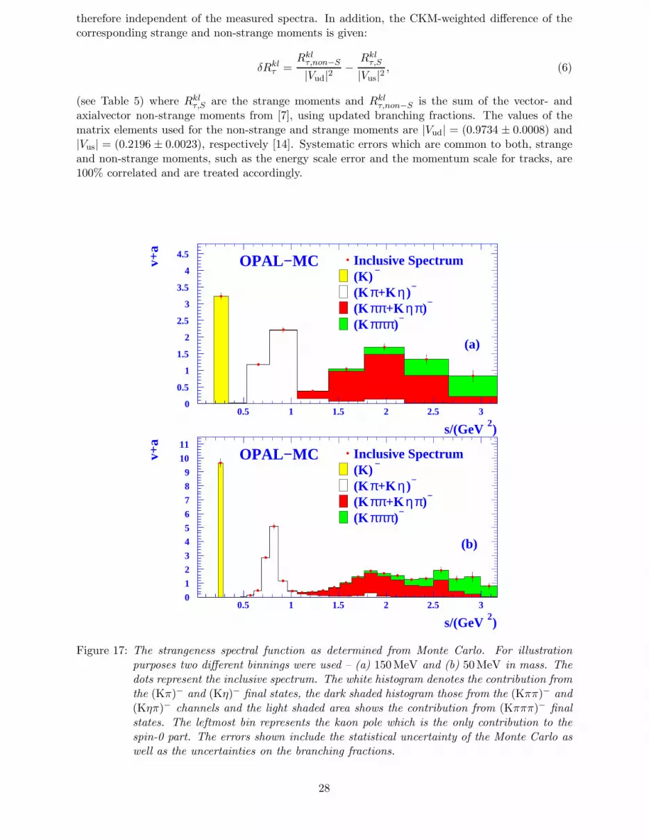
Summing the individual contributions (see Equations 3 and 4), the strangeness spectral functionis obtained. The Monte Carlo prediction of the total strangeness spectral function as a function ofthe invariant mass squared is displayed in Figure 17. The improved version of the τ Monte Carloas explained in Section 2.3 has been used here. The branching fractions as given in Table 1 havebeen used to weight the individual mass spectra. For illustration purposes the spectral function isshown using two different binnings. A non-equidistant binning is chosen which corresponds to abin width of 50MeV and 150MeV in the invariant mass, respectively. The errors given here arefrom Monte Carlo statistics only.
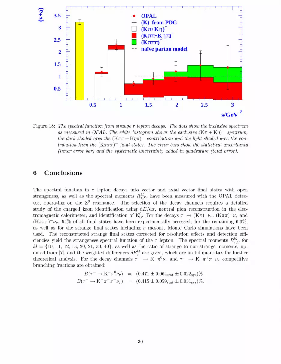
The spectral function obtained from the data is displayed in Figure 18. For τ− → K−π0ντ andτ− → K−π+π−ντ , the new average branching fractions and their respective errors as given inSection 5.2 are used. The binning chosen in this plot corresponds to a bin width of 150MeV in theinvariant mass and is governed by the mass resolution of the K0π−π0ντ final state. The dots witherror bars represent the inclusive spectrum. The inner error bars are the statistical uncertainties.They include the uncertainty on the efficiency and on Monte Carlo statistics. The total error iscalculated by adding up the statistical and systematic uncertainties (explained in the next section)in quadrature. The numerical values are given in Table 4. The systematic uncertainty is dominatedby the uncertainty on the τ branching fractions.
For the (Kπ)− final state both τ decay channels K0π−ντ and K−π0ντ are measured. The channelK−ηντ which also contributes to the two meson final state is taken from Monte Carlo. For the(Kππ)− final state the spectra K0π−π0ντ and K−π+π−ντ are measured. The contribution fromthe decay K−π0π0ντ is added from Monte Carlo as well as the K−ηπ0ντ channel which also con-tributes to the three meson final states. For the (Kπππ)− spectrum, which consists of the channelsK−π+π−π0ντ , K0π−π0π0ντ , K−π0π0π0ντ and K0π−π+π−ντ , the prediction from the Monte Carlois taken.
5.4 Systematic Uncertainties on the Spectral Function
The sources for possible systematic uncertainties listed below have been considered. Since theindividual contributions are different for the different final states, the error is given for each bin ins separately in Table 4.� Energy loss measurement (∆dE/dx):
The systematic variation is described in Section 5.1. In addition, the momentum dependenceof this variation has been investigated. No significant influence has been found.� Energy scale in π0 reconstruction (∆E):The systematic variation is described in Section 5.1.� Momentum scale (∆p):The systematic variation is described in Section 5.1.� PDG errors on branching fractions (∆B):The dominant contribution to the systematic uncertainty comes from the uncertainty in the
26
τ branching fractions (see Table 1). The branching fractions are varied randomly and thedifference in the result is quoted as systematic uncertainty. The channels which populate theregion of high s have branching fractions with relative errors close to 100% leading to largeuncertainty in the spectral function itself. This also covers the uncertainties on the shape.� K0
S identification (∆K0
S
):
A possible origin for systematic effects in the K0S identification is the estimation of the back-
ground using Monte Carlo. In particular the number of photon conversions found in τ leptondecays is not perfectly modeled. The cut on the χ2 probability of the 2C constrained fit to K0
S
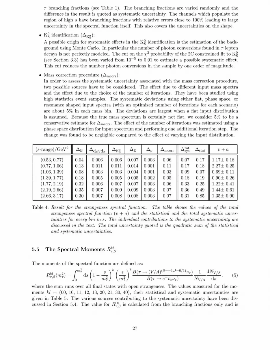
(see Section 3.3) has been varied from 10−5 to 0.01 to estimate a possible systematic effect.This cut reduces the number photon conversions in the sample by one order of magnitude.� Mass correction procedure (∆mcorr):In order to assess the systematic uncertainty associated with the mass correction procedure,two possible sources have to be considered. The effect due to different input mass spectraand the effect due to the choice of the number of iterations. They have been studied usinghigh statistics event samples. The systematic deviations using either flat, phase space, orresonance shaped input spectra (with an optimized number of iterations for each scenario)are about 5% in each mass bin. The deviations are largest when a flat input distributionis assumed. Because the true mass spectrum is certainly not flat, we consider 5% to be aconservative estimate for ∆mcorr. The effect of the number of iterations was estimated using aphase space distribution for input spectrum and performing one additional iteration step. Thechange was found to be negligible compared to the effect of varying the input distribution.
(s-range)/GeV2 ∆B ∆dE/dx ∆K0
S
∆E ∆p ∆mcorr ∆totsys ∆stat v + a
(0.53, 0.77) 0.04 0.006 0.006 0.007 0.003 0.06 0.07 0.17 1.17± 0.18(0.77, 1.06) 0.13 0.011 0.011 0.014 0.001 0.11 0.17 0.18 2.27± 0.25(1.06, 1.39) 0.08 0.003 0.003 0.004 0.001 0.03 0.09 0.07 0.69± 0.11(1.39, 1.77) 0.18 0.005 0.005 0.005 0.002 0.05 0.18 0.19 0.90± 0.26(1.77, 2.19) 0.32 0.006 0.007 0.007 0.003 0.06 0.33 0.25 1.22± 0.41(2.19, 2.66) 0.35 0.007 0.009 0.009 0.003 0.07 0.36 0.49 1.44± 0.61(2.66, 3.17) 0.30 0.007 0.008 0.008 0.003 0.07 0.31 0.85 1.35± 0.90
Table 4: Result for the strangeness spectral function. The table shows the values of the totalstrangeness spectral function (v + a) and the statistical and the total systematic uncer-tainties for every bin in s. The individual contributions to the systematic uncertainty arediscussed in the text. The total uncertainty quoted is the quadratic sum of the statisticaland systematic uncertainties.
5.5 The Spectral Moments Rklτ,S
The moments of the spectral function are defined as:
Rklτ,S(m2
τ ) =
∫ m2τ
0ds
(1 − s
m2τ
)k (s
m2τ
)l B(τ → (V/A)(S=−1,J=0/1)ντ )
B(τ → e−νeντ )
1
NV/A
dNV/A
ds, (5)
where the sum runs over all final states with open strangeness. The values measured for the mo-ments kl = (00, 10, 11, 12, 13, 20, 21, 30, 40), their statistical and systematic uncertainties aregiven in Table 5. The various sources contributing to the systematic uncertainty have been dis-cussed in Section 5.4. The value for R00
τ,S is calculated from the branching fractions only and is
27
therefore independent of the measured spectra. In addition, the CKM-weighted difference of thecorresponding strange and non-strange moments is given:
δRklτ =
Rklτ,non−S
|Vud|2−
Rklτ,S
|Vus|2, (6)
(see Table 5) where Rklτ,S are the strange moments and Rkl
τ,non−S is the sum of the vector- andaxialvector non-strange moments from [7], using updated branching fractions. The values of thematrix elements used for the non-strange and strange moments are |Vud| = (0.9734 ± 0.0008) and|Vus| = (0.2196 ± 0.0023), respectively [14]. Systematic errors which are common to both, strangeand non-strange moments, such as the energy scale error and the momentum scale for tracks, are100% correlated and are treated accordingly.
Inclusive Spectrum(K) −
(K π+K η )−
(K ππ+K ηπ)−
(K πππ)−
OPAL−MC
s/(GeV 2)
v+a
0
0.5
1
1.5
2
2.5
3
3.5
4
4.5
0.5 1 1.5 2 2.5 3
(a)
Inclusive Spectrum(K) −
(K π+K η )−
(K ππ+K ηπ)−
(K πππ)−
OPAL−MC
s/(GeV 2)
v+a
0
1
2
3
4
5
6
7
8
9
10
11
0.5 1 1.5 2 2.5 3
(b)
Figure 17: The strangeness spectral function as determined from Monte Carlo. For illustrationpurposes two different binnings were used – (a) 150MeV and (b) 50MeV in mass. Thedots represent the inclusive spectrum. The white histogram denotes the contribution fromthe (Kπ)− and (Kη)− final states, the dark shaded histogram those from the (Kππ)− and(Kηπ)− channels and the light shaded area shows the contribution from (Kπππ)− finalstates. The leftmost bin represents the kaon pole which is the only contribution to thespin-0 part. The errors shown include the statistical uncertainty of the Monte Carlo aswell as the uncertainties on the branching fractions.
28

kl Rklτ,non−S 00 10 11 12 13 20 21 30 40
00 3.469±0.014 10010 2.493±0.013 66 10011 0.549±0.004 68 65 10012 0.203±0.002 51 9 74 10013 0.092±0.002 33 -26 33 86 10020 1.944±0.011 55 93 45 -11 -40 10021 0.346±0.003 59 86 88 35 -13 71 10030 1.597±0.009 48 85 28 -24 -44 93 58 10040 1.362±0.008 42 77 14 -30 -43 87 43 92 100
kl Rklτ,S ∆stat ∆dE/dx ∆K0
S∆E ∆p ∆mcorr 00 10 11 12 13 20 21 30 40
00 0.1677±0.0050 – – – – – – 10010 0.1161±0.0038 0.0035 0.0006 0.0006 0.0005 0.0002 0.0011 89 10011 0.0298±0.0012 0.0011 0.0001 0.0001 0.0001 0.0001 0.0004 97 83 10012 0.0107±0.0006 0.0005 0.0002 0.0002 0.0002 0.0001 0.0002 86 54 91 10013 0.0048±0.0004 0.0002 0.0002 0.0002 0.0002 0.0001 0.0001 74 36 78 97 10020 0.0862±0.0028 0.0025 0.0006 0.0006 0.0006 0.0002 0.0008 75 97 66 32 13 10021 0.0191±0.0007 0.0006 0.0001 0.0001 0.0001 0.0001 0.0002 92 96 92 66 47 87 10030 0.0671±0.0022 0.0020 0.0005 0.0005 0.0004 0.0002 0.0006 66 92 54 19 1 99 78 10040 0.0539±0.0018 0.0016 0.0003 0.0003 0.0003 0.0001 0.0005 60 87 46 11 -4 96 70 99 100
kl δRklτ 00 10 11 12 13 20 21 30 40
00 0.184 ± 0.128 10010 0.224 ± 0.095 79 10011 -0.039±0.028 88 67 10012 -0.008±0.014 67 37 65 10013 -0.002±0.009 49 20 48 53 10020 0.264 ± 0.070 64 74 51 20 5 10021 -0.031±0.017 81 76 75 46 26 66 10030 0.294 ± 0.055 56 71 42 11 0 73 60 10040 0.320 ± 0.045 52 69 36 6 -4 74 55 77 100
kl Rklτ,S/Rkl
τ,non−S 00 10 11 12 13 20 21 30 40
00 0.0484±0.0015 10010 0.0466±0.0015 79 10011 0.0543±0.0022 88 67 10012 0.0527±0.0030 67 37 66 10013 0.0518±0.0045 49 20 48 53 10020 0.0444±0.0015 64 74 51 20 5 10021 0.0552±0.0021 80 76 75 46 26 66 10030 0.0420±0.0014 57 71 42 12 0 73 59 10040 0.0400±0.0013 53 69 36 7 -4 73 55 76 100
Table 5: The spectral moments for kl = (00, 10, 11, 12, 13, 20, 21, 30, 40). The tables include the values for the non-strange moments, the strangemoments, the weighted difference and the quotient of strange to non-strange moments. The values for the non-strange moments given arecalculated from [7] using updated branching fractions. For the strange moments, statistical and systematic uncertainties are listed separatelyfor the individual sources. The statistical uncertainty also contains the uncertainty on the branching fractions. The uncertainty on R00
τ isthe total error from the branching fractions as given in [14]. On the right hand side of each table, the correlations are given in percent.
29
OPAL(K) from PDG−
(K π+K η)−
(K ππ+K ηπ)−
(K πππ)−
naïve parton model
s/GeV2
(v+
a)
0.5
1
1.5
2
2.5
3
3.5
0.5 1 1.5 2 2.5 3
Figure 18: The spectral function from strange τ lepton decays. The dots show the inclusive spectrumas measured in OPAL. The white histogram shows the exclusive (Kπ + Kη)− spectrum,the dark shaded area the (Kππ + Kηπ)− contribution and the light shaded area the con-tribution from the (Kπππ)− final states. The error bars show the statistical uncertainty(inner error bar) and the systematic uncertainty added in quadrature (total error).
6 Conclusions
The spectral function in τ lepton decays into vector and axial vector final states with openstrangeness, as well as the spectral moments Rkl
τ,S , have been measured with the OPAL detec-
tor, operating on the Z0 resonance. The selection of the decay channels requires a detailedstudy of the charged kaon identification using dE/dx, neutral pion reconstruction in the elec-tromagnetic calorimeter, and identification of K0
S. For the decays τ−→ (Kπ)−ντ , (Kππ)−ντ and(Kπππ)−ντ , 94% of all final states have been experimentally accessed; for the remaining 6.6%,as well as for the strange final states including η mesons, Monte Carlo simulations have beenused. The reconstructed strange final states corrected for resolution effects and detection effi-ciencies yield the strangeness spectral function of the τ lepton. The spectral moments Rkl
τ,S forkl = {10, 11, 12, 13, 20, 21, 30, 40}, as well as the ratio of strange to non-strange moments, up-dated from [7], and the weighted differences δRkl
τ are given, which are useful quantities for furthertheoretical analysis. For the decay channels τ− → K−π0ντ and τ− → K−π+π−ντ competitivebranching fractions are obtained:
B(τ− → K−π0ντ ) = (0.471 ± 0.064stat ± 0.022sys)%
B(τ− → K−π+π−ντ ) = (0.415 ± 0.059stat ± 0.031sys)%.
30
Acknowledgements:
We particularly wish to thank the SL Division for the efficient operation of the LEP accelerator atall energies and for their close cooperation with our experimental group. In addition to the supportstaff at our own institutions we are pleased to acknowledge theDepartment of Energy, USA,National Science Foundation, USA,Particle Physics and Astronomy Research Council, UK,Natural Sciences and Engineering Research Council, Canada,Israel Science Foundation, administered by the Israel Academy of Science and Humanities,Benoziyo Center for High Energy Physics,Japanese Ministry of Education, Culture, Sports, Science and Technology (MEXT) and a grantunder the MEXT International Science Research Program,Japanese Society for the Promotion of Science (JSPS),German Israeli Bi-national Science Foundation (GIF),Bundesministerium fur Bildung und Forschung, Germany,National Research Council of Canada,Hungarian Foundation for Scientific Research, OTKA T-038240, and T-042864,The NWO/NATO Fund for Scientific Research, the Netherlands.
References
[1] E. Braaten, S. Narison and A. Pich, Nucl. Phys. B373, (1992) 581.
[2] E. Braaten, Phys. Rev. Lett. 60, (1988) 1606.
[3] E. Braaten, Phys. Rev. D39, (1989) 1458.
[4] S. Narison and A. Pich, Phys. Lett. B211, (1988) 183.
[5] F. Le Diberder and A. Pich, Phys. Lett. B286, (1992) 147.
[6] A. A. Pivovarov, Z. Phys. C 53, (1992) 461.
[7] OPAL Collaboration, K. Ackerstaff et al., Eur. Phys. J. C7, (1999) 571.
[8] ALEPH Collaboration, R. Barate et al., Eur. Phys. J. C4, (1998) 409.
[9] CLEO Collaboration, T. Coan et al., Phys. Lett. B356, (1995) 580.
[10] See for example A. Pich, ‘QCD predictions for the tau hadronic width: Determination ofαs(mτ )’ in Proceedings of the 2nd Workshop on Tau Lepton Physics, edited by K. K. Ghan,Columbus, Ohio, 1992.
[11] K. G. Chetyrkin, J. H. Kuhn and A. A. Pivovarov, Nucl. Phys. B 533, (1998) 473.
[12] A. Pich and J. Prades, JHEP 9910, (1999) 004.
[13] K. Maltman, eConf C0209101, (2002) WE05.
[14] K. Hagiwara et al., Phys. Rev. D 66, (2002) 010001 (URL: http://pdg.lbl.gov/2003/s035.pdf).
[15] OPAL Collaboration, G. Abbiendi et al., Eur. Phys. J. C13, (2000) 197.
[16] OPAL Collaboration, R. Akers et al., Phys. Lett. B328, (1994) 207.
31
[17] OPAL Collaboration, K. Ahmet et al., Nucl. Instr. and Meth. A 305, (1991) 275.
[18] P.P. Allport et al., Nucl. Instr. and Meth. A 324, (1993) 34;P.P. Allport et al., Nucl. Instr. and Meth. A 346, (1994) 476.
[19] S. Jadach, B.F.L. Ward, and Z. Was, Comp. Phys. Comm. 79, (1994) 503.
[20] S. Jadach, Z. Was, R. Decker, and J.H. Kuhn, Comp. Phys. Comm. 76, (1993) 361.
[21] M. Finkemeier and E. Mirkes, Z. Phys. C 69, (1996) 243.
[22] M. Finkemeier, J. H. Kuhn and E. Mirkes, Nucl. Phys. Proc. Suppl. 55C, (1997) 169.
[23] J. Allison et al., Nucl. Instrum. Methods A317, (1992) 47.
[24] T. Sjostrand, Comp. Phys. Comm. 82, (1994) 74.
[25] S. Jadach, W. Placzek and B. F. Ward, Phys. Lett. B 390, (1997) 298.
[26] R. Engel, and J. Ranft Phys. Rev. D54, (1996) 4244.
[27] A. Buijs, W. G. Langeveld, M. H. Lehto and D. J. Miller, Comput. Phys. Commun. 79, (1994)523.
[28] R. Battacharya, J. Smith, and G. Grammer, Phys. Rev. D15, (1977) 3267.
[29] J. Smith, J.A.M. Vermaseren, and G. Grammer, Phys. Rev. D15, (1977) 3280.
[30] M. Hauschild et al., Nucl. Inst. Meth. A314, (1992) 74.
[31] S. Bethke, Z. Kunszt, D.E. Soper and W.J. Stirling: Nucl. Phys. B370, (1992) 310, erratumibid. B523, (1998) 681.
[32] OPAL Collaboration ,G. Abbiendi et al., Eur. Phys. J. C 13, (2000) 197.
[33] CLEO Collaboration, R. A. Briere et al., Phys. Rev. Lett. 90, (2003) 181802.
[34] ALEPH Collaboration, R. Barate et al., Eur. Phys. J. C 1, (1998) 65.
[35] BES Collaboration, J.Z. Bai et al., Phys. Rev. D53, (1996) 20.
[36] W.J. Marciano and A. Sirlin, Phys. Rev. Lett. 61, (1988) 1815.
32


