University of Massachusetts - AmherstScholarWorks@UMass Amherst

Physics Department Faculty Publication Series Physics Department

2004

Hadronic parity violation: an overviewBR Holsteinholstein@physics.umass.edu

This Article is brought to you for free and open access by the Physics Department at ScholarWorks@UMass Amherst. It has been accepted forinclusion in Physics Department Faculty Publication Series by an authorized administrator of ScholarWorks@UMass Amherst. For more information,please contact scholarworks@library.umass.edu.

Holstein, BR, "Hadronic parity violation: an overview" (2004). Physics Department Faculty Publication Series. Paper 287.http://scholarworks.umass.edu/physics_faculty_pubs/287

arX

iv:n

ucl-

th/0

6070

38v1

18

Jul 2

006

Hadronic Parity Violation: an Analytic Approach

Barry R. Holstein

Department of Physics-LGRT

University of Massachusetts

Amherst, MA 01003

February 5, 2008

Abstract

Using a recent reformulation of the analysis of nuclear parity-violation(PV) using the framework of effective field theory (EFT), we show howpredictions for parity-violating observables in low energy light hadronicsystems can be understood in an analytic fashion. It is hoped that suchan analytic approach may encourage additional experimental work as wellas add to the understanding of such parity-violating phenomena, whichis all too often obscured by its description in terms of numerical resultsobtained from complex two-body potential codes.

1

1 Introduction

I never had the pleasure of meeting Dubravko Tadic , which is a shame, sincehe and I worked on many parallel subjects over the years. An example of this ishis recent work on hypernuclear decay[1] as well as his early papers on what isusually called nuclear parity violation[2]. It is the latter which I wish to focuson in this paper, which I dedicate to Dubravko’s memory.

The cornerstone of traditional nuclear physics is the study of nuclear forcesand, over the years, phenomenological forms of the nuclear potential have be-come increasingly sophisticated. In the nucleon-nucleon (NN) system, wheredata abound, the present state of the art is indicated, for example, by phe-nomenological potentials such as AV18 that are able to fit phase shifts in theenergy region from threshold to 350 MeV in terms of ∼ 40 parameters. Progresshas also been made in the description of few-nucleon systems [3]. At the sametime, in recent years a new technique —effective field theory (EFT)— has beenused in order to attack this problem using the symmetries of QCD [4]. Inthis approach the nuclear interaction is separated into long- and short-distancecomponents. In its original formulation [5], designed for processes with typicalmomenta comparable to the pion mass, Q ∼ mπ, the long-distance component isdescribed fully quantum mechanically in terms of pion exchange, while the short-distance piece is described in terms of a small number of phenomenologically-determined contact couplings. The resulting potential [6, 7] is approaching [8, 9]the degree of accuracy of purely-phenomenological potentials. Even higher pre-cision can be achieved at lower momenta, where all interations can be taken asshort-ranged, as has been demonstrated not only in the NN system [10, 11],but also in the three-nucleon system [12, 13]. Precise —∼ 1%— values havebeen generated also for low-energy, astrophysically-important cross sections forreactions such as n + p → d + γ [14] and p + p → d + e+ + νe[15]. However,besides providing reliable values for such quantities, the use of EFT techniquesallows for the a realistic estimation of the size of possible corrections.

Over the past nearly half century there has also developed a series of mea-surements attempting to illuminate the parity-violating (PV) nuclear interac-tion. Indeed the first experimental paper of which I am aware was that of Tannerin 1957 [16], shortly after the experimental confirmation of parity violation innuclear beta decay by Wu et al. [17]. Following seminal theoretical work byMichel in 1964 [18] and that of other authors in the late 1960’s [19, 20, 21], theresults of such experiments have generally been analyzed in terms of a meson-exchange picture, and in 1980 the work of Desplanques, Donoghue, and Holstein(DDH) developed a comprehensive and general meson-exchange framework forthe analysis of such interactions in terms of seven parameters representing weakparity-violating meson-nucleon couplings [22]. The DDH interaction has be-come the standard setting by which hadronic and nuclear PV processes are nowanalyzed theoretically.

It is important to observe, however, that the DDH framework is, at heart,a model based on a meson-exchange picture. Provided one is interested primar-ily in near-threshold phenomena, use of a model is unnecessary, and one can

1

instead represent the PV nuclear interaction in a model-independent effective-field-theoretic fashion, as recently developed by Zhu et al.[23]. In this approach,the low energy PV NN interaction is entirely short-ranged, and the most generalpotential depends at leading order on 11 independent operators parameterizedby a set of 11 a priori unknown low-energy constants (LEC’s). When applied tolow-energy (Ecm ≤ 50 MeV) two-nucleon PV observables, however, such as theneutron spin asymmetry in the capture reaction ~n+p→ d+γ, the 11 operatorsreduce to a set of five independent PV amplitudes which may be determined byan appropriate set of measurements, as described in [23], and an experimentalprogram which should result in the determination of these couplings is underway.This is an important goal, since such interactions are interesting not only in theirown right but also as background effects entering atomic PV measurements[24]as well as experiments that use parity violation in electromagnetic interactionsin order to probe nuclear structure[25].

Completion of such a low-energy program would serve at least three addi-tional purposes:

i) First, it would provide particle theorists with a set of five benchmark num-bers which are in principle explainable from first principles. This situationwould be analogous to what one encounters in chiral perturbation theoryfor pseudoscalars, where the experimental determination of the ten LEC’sappearing in the O(p4) Lagrangian presents a challenge to hadron struc-ture theory. While many of the O(p4) LEC’s are saturated by t-channelexchange of vector mesons, it is not clear a priori that the analogous PVNN constants are similarly saturated (as assumed implicitly in the DDHmodel).

ii) Moreover, analysis of the PV NN LEC’s involves the interplay of weakand strong interactions in the strangeness conserving sector. A similarsituation occurs in ∆S = 1 hadronic weak interactions, and the interplayof strong and weak interactions in this case are both subtle and onlypartially understood, as evidenced, e.g., by the well-known the ∆I = 1/2rule enigma. The additional information in the ∆S = 0 sector providedby a well-defined set of experimental numbers would undoubtedly shedlight on this fundamental problem.

iii) Finally, the information derived from the low-energy nuclear PV programwould also provide a starting point for a reanalysis of PV effects in many-body systems. Until now, one has attempted to use PV observables ob-tained from both few- and many-body systems in order to determine theseven PV meson-nucleon couplings entering the DDH potential, and sev-eral inconsistencies have emerged. The most blatant is the vastly differentvalue for hπ obtained from the PV γ-decays of 18F, 19F and from the com-bination of the ~pp asymmetry and the cesium anapole moment[24]. Theorigin of this clash could be due to any one of a number of factors. Usingthe operator constraints derived from the few-body program as input into

2

the nuclear analysis could help clarify the situation. It may be, for exam-ple, that the remaining combinations of operators not constrained by thefew-body program play a more significant role in nuclei than implicitlyassumed by the DDH framework. Alternatively, truncation of the modelspace in shell model treatments of the cesium anapole moment may bethe culprit. In any case, approaching the nuclear problem from a moresystematic perspective and drawing upon the results of few-body studieswould undoubtedly represent an advance for the field.

The purpose of the present paper is not, however, to make the case for theeffective field theory program—this has already been undertaken in [23]. Also,it is not our purpose to review the subject of hadronic parity violation—indeedthere exist a number of comprehensive recent reviews of this subject[26][27][28].However, although the basic ideas of the physics are clearly set out in theseworks, because the NN interaction is generally represented in terms of a some-what forbidding two-body interaction, any calculations which are done involvestate of the art potentials and are somewhat mysterious except to those priestswho preach this art. Rather, in this paper, we wish to argue that this need notbe the case. Below we eschew a high precision but complex nuclear wavefunc-tion approach in favor of a simple analytic treatment which captures the flavorof the subject without the complications associated with a more rigorous cal-culation. We show that, provided that one is working in the low energy region,one can use a simple effective interaction approach to the PV NN interactionwherein the the parity violating NN interaction is described in terms of just fivereal numbers, which characterize S-P wave mixing in the spin singlet and tripletchannels, and the experimental and theoretical implications can be extractedwithin a basic effective interaction technique, wherein the nucleon interactionsare represented by short range potentials. This is justified at low energy becausethe scales indicated by the scattering lengths—as ∼ −20 fm, at ∼ 5 fm—areboth much larger than the ∼ 1 fm range of the nucleon-nucleon strong inter-action. Of course, precision analysis should still be done with the best andmost powerful contemporary wavefunctions such as the Argonne V18 or Bonnpotentials. Nevertheless, for a simple introduction to the field, we feel that theelementary discussion given below is didactically and motivationally useful. Inthe next section then we present a brief review of the standard DDH formalism,since this is the basis of most analysis, as well as the EFT picture in which weshall work. Then in the following section we show how the basic physics of theNN system can be elicited in a simple analytic fashion, focusing in particularon the deuteron. With this as a basis we proceed to the parity-violating NN in-teraction and develop a simple analytic description of low energy PV processes.We summarize out findings in a brief concluding section

2 Hadronic Parity Violation: Old and New

The essential idea behind the conventional DDH framework relies on the fairlysuccessful representation of the parity-conserving NN interaction in terms of a

3

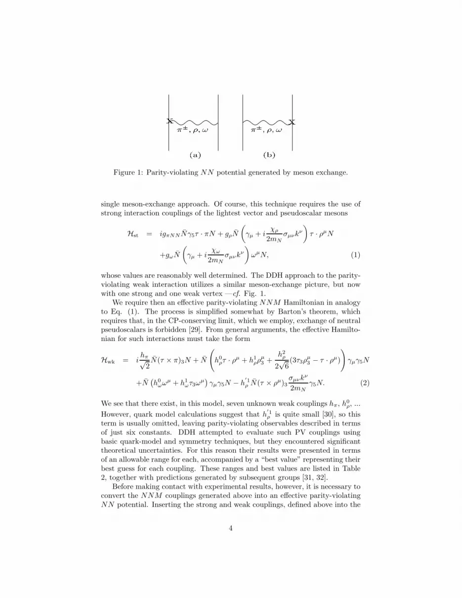
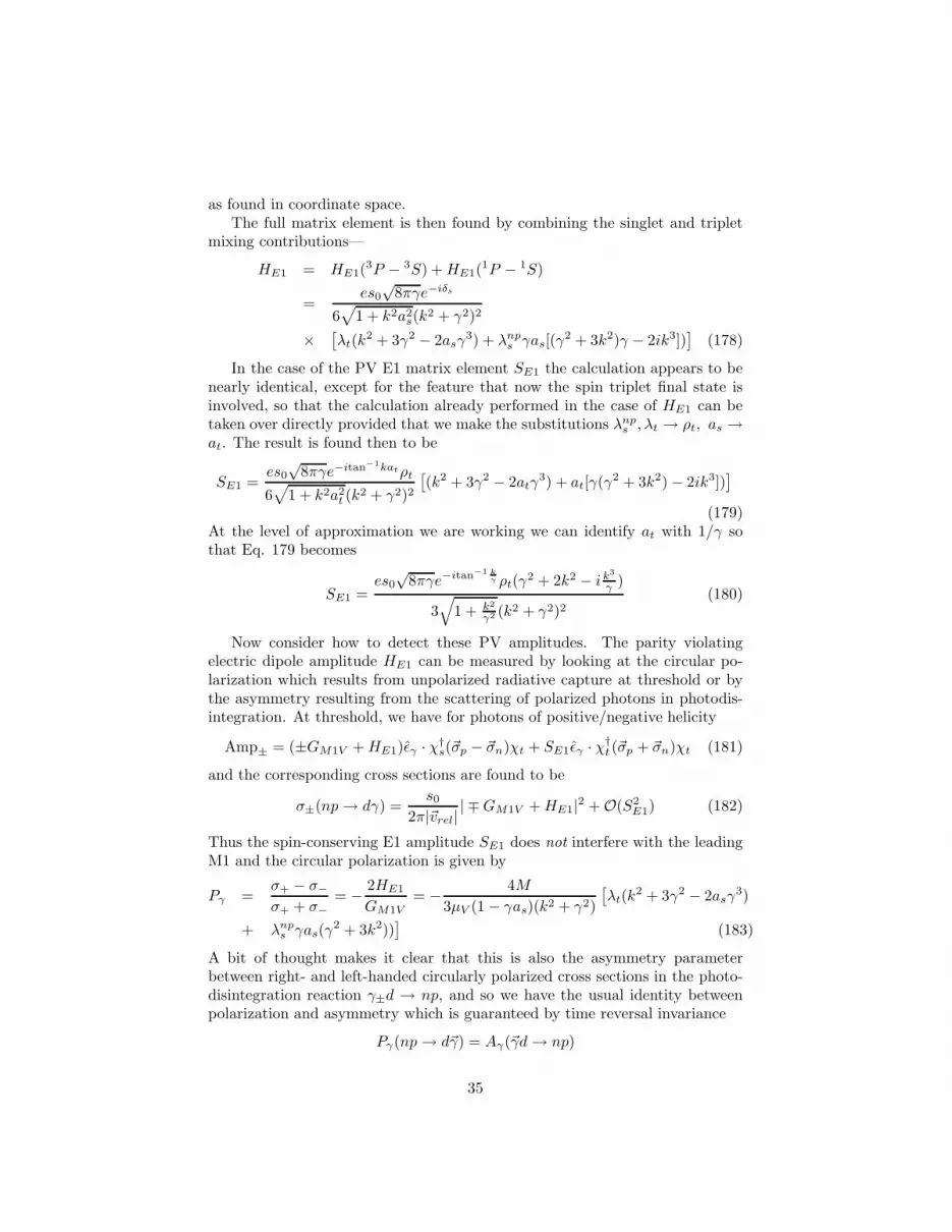
; ; !X (a) ; ; ! X(b)Figure 1: Parity-violating NN potential generated by meson exchange.

single meson-exchange approach. Of course, this technique requires the use ofstrong interaction couplings of the lightest vector and pseudoscalar mesons

Hst = igπNNNγ5τ · πN + gρN

(

γµ + iχρ

2mN

σµνkν

)

τ · ρµN

+gωN

(

γµ + iχω

2mN

σµνkν

)

ωµN, (1)

whose values are reasonably well determined. The DDH approach to the parity-violating weak interaction utilizes a similar meson-exchange picture, but nowwith one strong and one weak vertex —cf. Fig. 1.

We require then an effective parity-violating NNM Hamiltonian in analogyto Eq. (1). The process is simplified somewhat by Barton’s theorem, whichrequires that, in the CP-conserving limit, which we employ, exchange of neutralpseudoscalars is forbidden [29]. From general arguments, the effective Hamilto-nian for such interactions must take the form

Hwk = ihπ√

2N(τ × π)3N + N

(

h0ρτ · ρµ + h1

ρρµ3 +

h2ρ

2√

6(3τ3ρ

µ3 − τ · ρµ)

)

γµγ5N

+N(

h0ωω

µ + h1ωτ3ω

µ)

γµγ5N − h′1ρ N(τ × ρµ)3

σµνkν

2mN

γ5N. (2)

We see that there exist, in this model, seven unknown weak couplings hπ, h0ρ, ...

However, quark model calculations suggest that h′1ρ is quite small [30], so this

term is usually omitted, leaving parity-violating observables described in termsof just six constants. DDH attempted to evaluate such PV couplings usingbasic quark-model and symmetry techniques, but they encountered significanttheoretical uncertainties. For this reason their results were presented in termsof an allowable range for each, accompanied by a “best value” representing theirbest guess for each coupling. These ranges and best values are listed in Table2, together with predictions generated by subsequent groups [31, 32].

Before making contact with experimental results, however, it is necessary toconvert the NNM couplings generated above into an effective parity-violatingNN potential. Inserting the strong and weak couplings, defined above into the

4

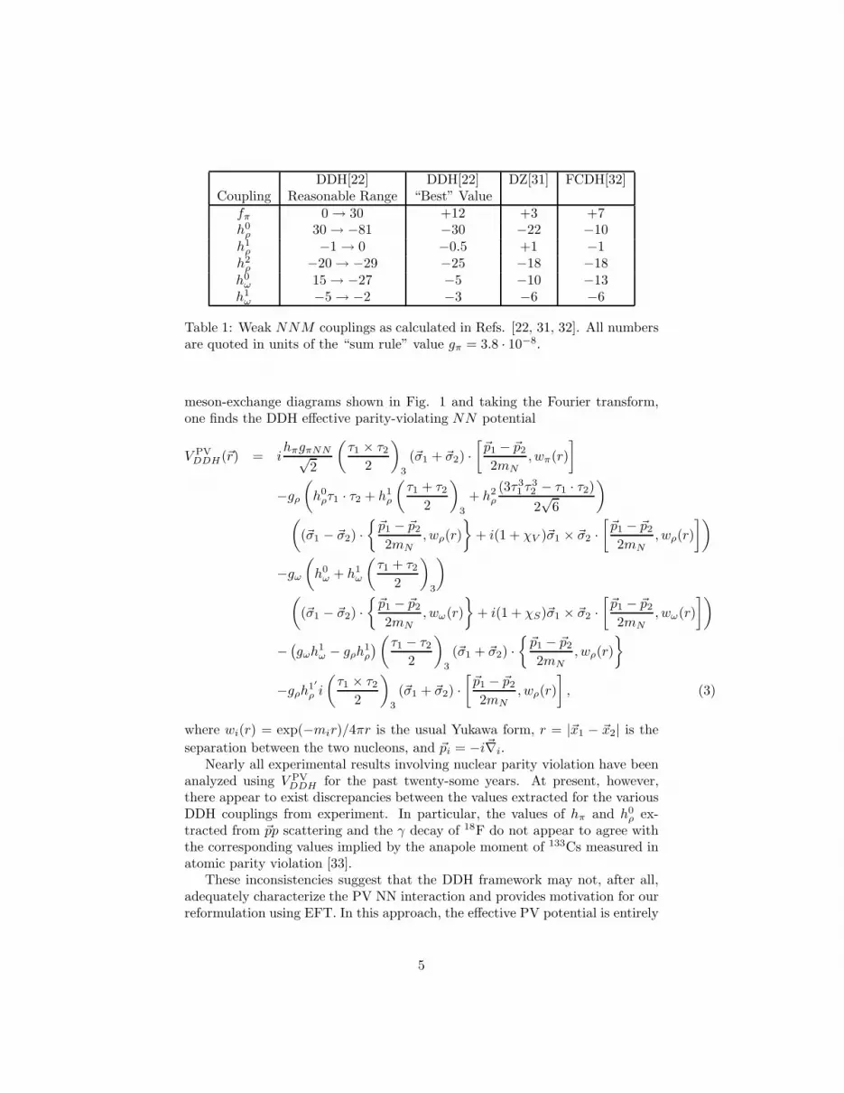
DDH[22] DDH[22] DZ[31] FCDH[32]Coupling Reasonable Range “Best” Value

fπ 0 → 30 +12 +3 +7h0

ρ 30 → −81 −30 −22 −10h1

ρ −1 → 0 −0.5 +1 −1h2

ρ −20 → −29 −25 −18 −18h0

ω 15 → −27 −5 −10 −13h1

ω −5 → −2 −3 −6 −6

Table 1: Weak NNM couplings as calculated in Refs. [22, 31, 32]. All numbersare quoted in units of the “sum rule” value gπ = 3.8 · 10−8.

meson-exchange diagrams shown in Fig. 1 and taking the Fourier transform,one finds the DDH effective parity-violating NN potential

V PVDDH(~r) = i

hπgπNN√2

(

τ1 × τ22

)

3

(~σ1 + ~σ2) ·[

~p1 − ~p2

2mN

, wπ(r)

]

−gρ

(

h0ρτ1 · τ2 + h1

ρ

(

τ1 + τ22

)

3

+ h2ρ

(3τ31 τ

32 − τ1 · τ2)

2√

6

)

(

(~σ1 − ~σ2) ·

~p1 − ~p2

2mN

, wρ(r)

+ i(1 + χV )~σ1 × ~σ2 ·[

~p1 − ~p2

2mN

, wρ(r)

])

−gω

(

h0ω + h1

ω

(

τ1 + τ22

)

3

)

(

(~σ1 − ~σ2) ·

~p1 − ~p2

2mN

, wω(r)

+ i(1 + χS)~σ1 × ~σ2 ·[

~p1 − ~p2

2mN

, wω(r)

])

−(

gωh1ω − gρh

1ρ

)

(

τ1 − τ22

)

3

(~σ1 + ~σ2) ·

~p1 − ~p2

2mN

, wρ(r)

−gρh1′

ρ i

(

τ1 × τ22

)

3

(~σ1 + ~σ2) ·[

~p1 − ~p2

2mN

, wρ(r)

]

, (3)

where wi(r) = exp(−mir)/4πr is the usual Yukawa form, r = |~x1 − ~x2| is the

separation between the two nucleons, and ~pi = −i~∇i.Nearly all experimental results involving nuclear parity violation have been

analyzed using V PVDDH for the past twenty-some years. At present, however,

there appear to exist discrepancies between the values extracted for the variousDDH couplings from experiment. In particular, the values of hπ and h0

ρ ex-tracted from ~pp scattering and the γ decay of 18F do not appear to agree withthe corresponding values implied by the anapole moment of 133Cs measured inatomic parity violation [33].

These inconsistencies suggest that the DDH framework may not, after all,adequately characterize the PV NN interaction and provides motivation for ourreformulation using EFT. In this approach, the effective PV potential is entirely

5

short-ranged and has the co-ordinate space form

V PVeff (~r) =

2

Λ3χ

[

C1 + C2τz1 + τz

2

2

]

(~σ1 − ~σ2) · −i~∇, fm(r)

+

[

C1 + C2τz1 + τz

2

2

]

i (~σ1 × ~σ2) · [−i~∇, fm(r)]

+ [C2 − C4]τz1 − τz

2

2(~σ1 + ~σ2) · −i~∇, fm(r)

+

[

C3τ1 · τ2 + C4τz1 + τz

2

2+ IabC5τ

a1 τ

b2

]

(~σ1 − ~σ2) · −i~∇, fm(r)

+

[

C3τ1 · τ2 + C4τz1 + τz

2

2+ IabC5τ

a1 τ

b2

]

i (~σ1 × ~σ2) · [−i~∇, fm(r)]

+C6iǫab3τa

1 τb2 (~σ1 + ~σ2) · [−i~∇, fm(r)]

, (4)

where

Iab =

1 0 00 1 00 0 −2

, (5)

and fm(~r) is a function which

i) is strongly peaked, with width ∼ 1/m about r = 0, and

ii) approaches δ(3)(~r) in the zero width—m → ∞—limit.

A convenient form, for example, is the Yukawa-like function

fm(r) =m2

4πrexp(−mr) (6)

where m is a mass chosen to reproduce the appropriate short range effects.Actually, for the purpose of carrying out actual calculations, one could just aseasily use the momentum-space form of V PV

SR , thereby avoiding the use of fm(~r)altogether. Nevertheless, the form of Eq. 4 is useful when comparing with theDDH potential. For example, we observe that the same set of spin-space andisospin structures appear in both V PV

eff and the vector-meson exchange terms in

V PVDDH, though the relationship between the various coefficients in V PV

eff is moregeneral. In particular, the DDH model is tantamount to assuming

C1

C1=C2

C2= 1 + χω, (7)

C3

C3=C4

C4=C5

C5= 1 + χρ, (8)

and taking m ∼ mρ,mω, assumptions which may not be physically realistic.Nevertheless, if this ansatz is made, the EFT and DDH results coincide providedthe identifications

6

CDDH1 = −

Λ3χ

2mNm2ω

gωNNh0ω,

CDDH2 = −

Λ3χ

2mNm2ω

gωNNh1ω,

CDDH3 = −

Λ3χ

2mNm2ρ

gρNNh0ρ,

CDDH4 = −

Λ3χ

2mNm2ρ

gρNNh1ρ,

CDDH5 =

Λ3χ

4√

6mNm2ρ

gρNNh2ρ,

CDDH6 = −

Λ3χ

2mNm2ρ

gρNNh′1ρ .

are made[23].Before beginning our analysis of PV NN scattering, however, it is important

to review the analogous PC NN scattering case, since it is more familiar and itis a useful arena wherein to compare conventional and effective field theoreticmethods.

3 Parity Conserving NN Scattering

We begin our discussion with a brief review of conventional scattering theory[34].In the usual partial wave expansion, we can write the scattering amplitude as

f(θ) =∑

ℓ

(2ℓ+ 1)aℓ(k)Pℓ(cos θ) (9)

where aℓ(k) has the form

aℓ(k) =1

keiδ(k) sin δ(k) =

1

k cot δ(k) − ik(10)

3.1 Conventional Analysis

Working in the usual potential model approach, a general expression for thescattering phase shift δℓ(k) is[34]

sin δℓ(k) = −k∫ ∞

0

dr′r′jℓ(kr′)2mrV (r′)uℓ,k(r′) (11)

where mr is the reduced mass and

uℓ,k(r) = r cos δℓ(k)jℓ(kr) + kr

∫ r

0

dr′r′jℓ(kr′)nℓ(kr)uℓ,k(r′)2mrV (r′)

+ kr

∫ ∞

r

dr′r′jℓ(kr)nℓ(kr′)uℓ,k(r′)2mrV (r′) (12)

7

is the scattering wavefunction. At low energies one can characterize the analyticfunction k2ℓ+1 cot δ(k) via an effective range expansion[35]

k2ℓ+1 cot δℓ(k) = −1

a+

1

2rek

2 + . . . (13)

Then from Eq. 11 we can identify the scattering length as

aℓ =1

[(2ℓ+ 1)!!]2

∫ ∞

0

dr′(r′)2ℓ+22mrV (r′) + O(V 2) (14)

For simplicity, we consider only S-wave interactions. Then for neutron-protoninteractions, for example, one finds

as0 = −23.715 ± 0.015 fm, rs

0 = 2.73 ± 0.03 fm

at0 = 5.423 ± 0.005 fm, rt

0 = 1.73 ± 0.02 fm (15)

for scattering in the spin-singlet and spin-triplet channels respectively. Theexistence of a bound state EB = −γ2/2mr is indicated by the presence of a polealong the positive imaginary k-axis—i.e. γ > 0 under the analytic continuationk → iγ—

1

a0+

1

2r0γ

2 − γ = 0 (16)

We see from Eq. 15 that there is no bound state in the np spin-singlet channel,but in the spin-triplet system there exists a solution

κ =1 −

√

1 − 2rt0

at0

rt0

= 45.7 MeV, i.e. EB = −2.23 MeV (17)

corresponding to the deuteron.As a specific example, suppose we utilize a simple square well potential to

describe the interaction

V (r) =

−V0 r ≤ R0 r > R

(18)

For S-wave scattering the wavefunction in the interior and exterior regions canthen be written as

ψ(+)(r) =

Nj0(Kr) r ≤ RN ′(j0(kr) cos δ0 − n0(kr) sin δ0) r > R

(19)

where j0, n0 are spherical harmonics and the interior, exterior wavenumbersare given by k =

√2mrE, K =

√

2mr(E + V0) respectively. The connectionbetween the two forms can be made by matching logarithmic derivatives at theboundary, which yields

k cot δ ≃ − 1

R

[

1 +1

KRF (KR)

]

with F (x) = cotx− 1

x(20)

8

Making the effective range expansion—Eq 13—we find an expression for thescattering length

a0 = R

[

1 − tan(K0R)

K0R

]

where K0 =√

2mrV0 (21)

Note that for weak potentials—K0R << 1—this form agrees with the generalresult Eq. 14—

a0 =

∫ ∞

0

dr′r′22mrV (r′) = −2mr

3R3V0 + O(V 2

0 ) (22)

3.2 Coulomb Effects

When Coulomb interactions are included the analysis becomes somewhat morechallenging. Suppose first that only same charge (e.g., proton-proton) scatteringis considered and that, for simplicity, we describe the interaction in terms of apotential of the form

V (r) =

U(r) r < Rαr

r > R(23)

i.e. a strong attraction—U(r)—at short distances, in order to mimic the stronginteraction, and the repulsive Coulomb potential—α/r—at large distance, whereα ≃ 1/137 is the fine structure constant. The analysis of the scattering thenproceeds as above but with the replacement of the exterior spherical Besselfunctions by corresponding Coulomb wavefunctions F+

0 , G+0

j0(kr) → F+0 (r), n0(kr) → G+

0 (r) (24)

whose explicit form can be found in reference [36]. For our purposes we requireonly the form of these functions in the limit kr << 1—

F+0 (r)

kr<<1−→ C(η+(k))(1 +r

2aB

+ . . .)

G+0 (r)

kr<<1−→ − 1

C(η+(k))

1

kr

+ 2η+(k)

[

h(η+(k)) + 2γE − 1 + lnr

aB

]

+ . . .

(25)

Here γE = 0.577215.. is the Euler constant,

C2(x) =2πx

exp(2πx) − 1(26)

is the usual Coulombic enhancement factor, aB = 1/mrα is the Bohr radius,η+(k) = 1/2kaB, and

h(η+(k)) = ReH(iη+(k)) = η2+(k)

∞∑

n=1

1

n(n2 + η2+(k))

− ln η+(k) − γE (27)

9

where H(x) is the analytic function

H(x) = ψ(x) +1

2x− ln(x) (28)

Equating interior and exterior logarithmic derivatives we find

KF (KR) =cos δ0F

+0

′(R) − sin δ0G

+0

′(R)

cos δ0F+0 (R) − sin δ0G

+0 (R)

=k cot δ0C

2(η+(k)) 12aB

− 1R2

k cot δ0C2(η+(k)) + 1R

+ 1aB

[

h(η+(k)) − ln aB

R+ 2γE − 1

]

(29)

Since R << aB Eq. 29 can be written in the form

k cot δ0C2(η+(k)) +

1

aB

[

h(η+(k)) − lnaB

R+ 2γE − 1

]

≃ − 1

a0(30)

The scattering length aC in the presence of the Coulomb interaction is conven-tionally defined as[37]

k cot δ0C2(η+(k)) +

1

aB

h(η+(k)) = − 1

aC

+ . . . (31)

so that we have the relation

− 1

a0= − 1

aC

− 1

aB

(lnaB

R+ 1 − 2γE) (32)

between the experimental scattering length—aC—and that which would existin the absence of the Coulomb interaction—a0.

As an aside we note that, strictly speaking, a0 is not itself an observablesince the Coulomb interaction cannot be turned off. However, in the case ofthe pp interaction isospin invariance requires app

0 = ann0 so that one has the

prediction

− 1

ann0

= − 1

appC

− αMN (ln1

αMNR+ 1 − 2γE) (33)

While this is a model dependent result, Jackson and Blatt have shown, bytreating the interior Coulomb interaction perturbatively, that a version of thisresult with 1 − 2γE → 0.824 − 2γE is approximately valid for a wide rangeof strong interaction potentials[36] and the correction indicated in Eq. 33 isessential in restoring agreement between the widely discrepant—ann

0 = −18.8fm vs. app

C = −7.82 fm—values obtained experimentally.Returning to the problem at hand, the experimental scattering amplitude

can then be written as

f+C (k) =

e2iσ0C2(η+(k))

− 1aC

− 1aBh(η+(k)) − ikC2(η+(k))

=e2iσ0C2(η+(k))

− 1aC

− 1aBH(iη+(k))

(34)

where σ0 = argΓ(1 − iη+(k)) is the Coulomb phase.

10

3.3 Effective Field Theory Analysis

Identical results may be obtained using effective field theory (EFT) methodsand in many ways the derivation is clearer and more intuitive[38]. The basicidea here is that since we are only interested in interactions at very low energy,a scattering length description is quite adequate. From Eq. 22 we see that, atleast for weak potentials, the scattering length has a natural representation interms of the momentum space potential V (~p = 0)—

a0 =mr

2π

∫

d3rV (r) =mr

2πV (~p = 0) (35)

and it is thus natural to perform our analysis using a simple contact interation.First consider the situation that we have two particles A,B interacting only viaa local strong interaction, so that the effective Lagrangian can be written as

L =B∑

i=A

Ψ†i (i

∂

∂t+

~∇2

2mi

)Ψi − C0Ψ†AΨAΨ†

BΨB + . . . (36)

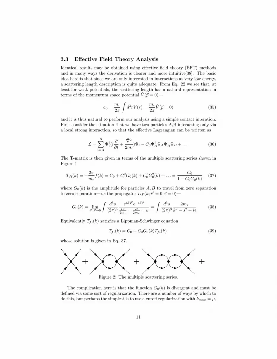
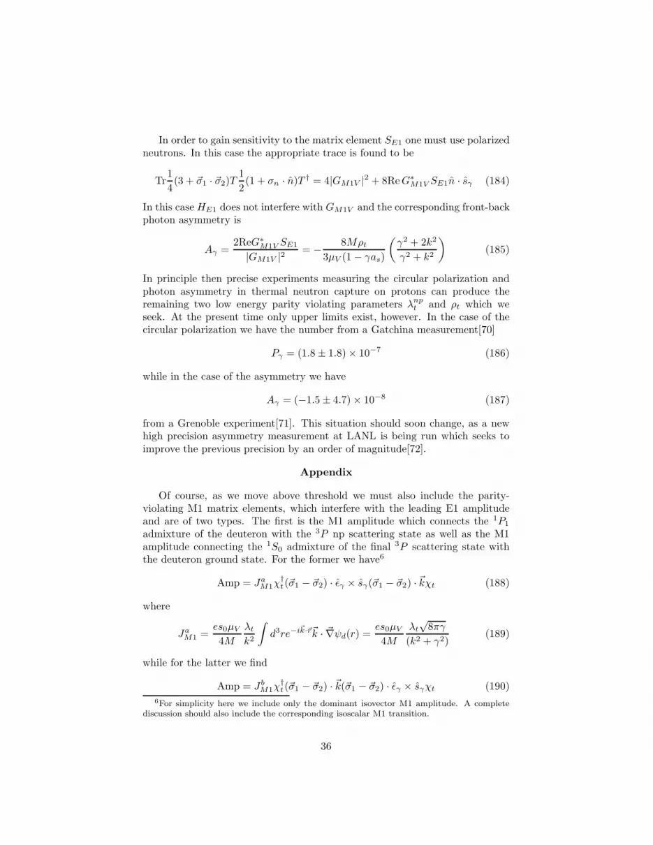
The T-matrix is then given in terms of the multiple scattering series shown inFigure 1

Tfi(k) = − 2π

mr

f(k) = C0 + C20G0(k) + C3

0G20(k) + . . . =

C0

1 − C0G0(k)(37)

where G0(k) is the amplitude for particles A,B to travel from zero separationto zero separation—i.e the propagator DF (k;~r′ = 0, ~r = 0)—

G0(k) = lim~r′,~r→0

∫

d3s

(2π)3ei~s·~r′

e−i~s·~r

k2

2mr− s2

2mr+ iǫ

=

∫

d3s

(2π)32mr

k2 − s2 + iǫ(38)

Equivalently Tfi(k) satisfies a Lippman-Schwinger equation

Tfi(k) = C0 + C0G0(k)Tfi(k). (39)

whose solution is given in Eq. 37.+++ . . .Figure 2: The multiple scattering series.

The complication here is that the function G0(k) is divergent and must bedefined via some sort of regularization. There are a number of ways by which todo this, but perhaps the simplest is to use a cutoff regularization with kmax = µ,

11

which simply eliminates the high momentum components of the wavefunctioncompletely. Then

G0(k) = −mr

2π(2µ

π+ ik) (40)

(Other regularization schemes are similar. For example, one could subtract atan unphysical momentum point, as proposed by Gegelia[39]

G0(k) =

∫

d3s

(2π)3(

2mr

k2 − s2 + iǫ+

2mr

µ2 + s2) = −mr

2π(µ+ ik) (41)

which has been shown by Mehen and Stewart[40] to be equivalent to the powerdivergence subtraction (PDS) scheme proposed by Kaplan, Savage and Wise.[38])In any case, the would-be linear divergence is, of course, cancelled by introduc-tion of a counterterm accounting for the omitted high energy component of thetheory, which renormalizes C0 to C0(µ). That C0(µ) should be a function of thecutoff is clear because by varying the cutoff energy we are varying the amountof higher energy physics which we are including in our effective description. Thescattering amplitude then becomes

f(k) = −mr

2π

(

11

C0(µ) −G0(k)

)

=1

− 2πmrC0(µ) −

2µπ

− ik(42)

Comparing with Eq. 10 we identify the scattering length as

− 1

a0= − 2π

mrC0(µ)− 2µ

π(43)

Of course, since a0 is a physical observable, it is cutoff independent, so that theµ dependence of 1/C0(µ) is cancelled by the cutoff dependence in the Green’sfunction.

3.4 Coulomb Effects in EFT

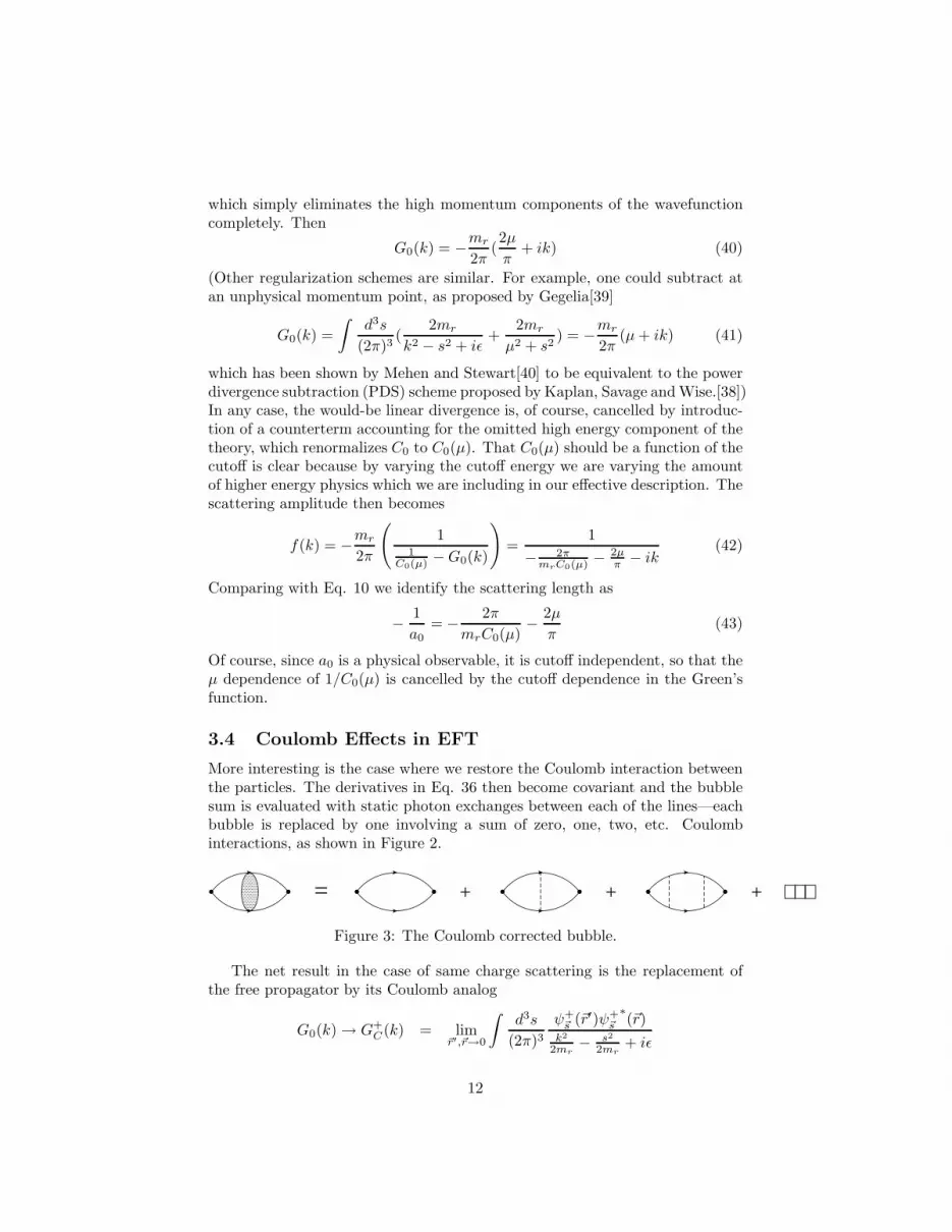
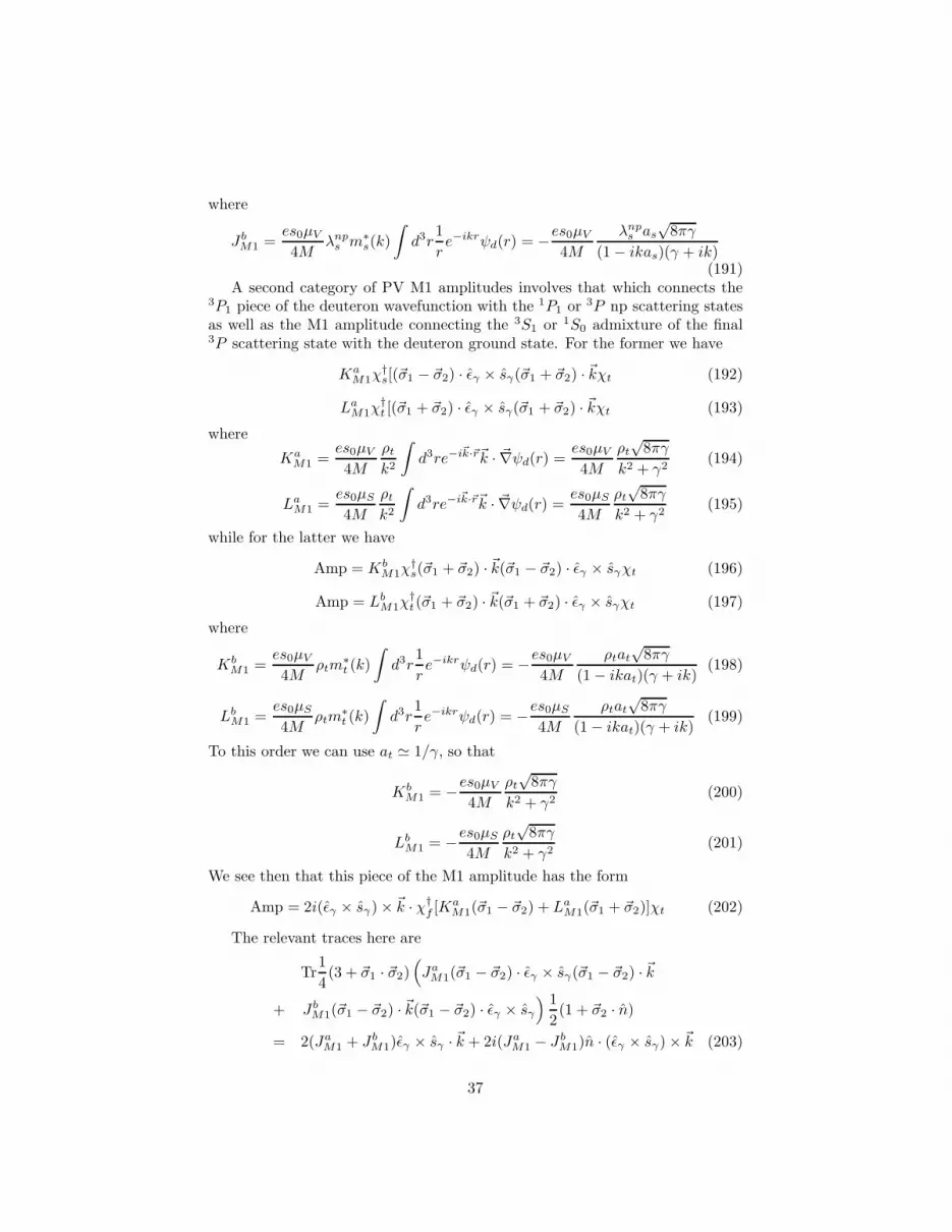
More interesting is the case where we restore the Coulomb interaction betweenthe particles. The derivatives in Eq. 36 then become covariant and the bubblesum is evaluated with static photon exchanges between each of the lines—eachbubble is replaced by one involving a sum of zero, one, two, etc. Coulombinteractions, as shown in Figure 2.

= + + + ⋅ ⋅ ⋅

Figure 3: The Coulomb corrected bubble.

The net result in the case of same charge scattering is the replacement ofthe free propagator by its Coulomb analog

G0(k) → G+C(k) = lim

~r′,~r→0

∫

d3s

(2π)3ψ+

~s (~r′)ψ+~s

∗(~r)

k2

2mr− s2

2mr+ iǫ

12

=

∫

d3s

(2π)32mrC

2(η+(s))

k2 − s2 + iǫ(44)

whereψ+

~s (~r) = C(η+(s))eiσ0ei~s·~r1F1(−iη+(s), 1, isr − i~s · ~r) (45)

is the outgoing Coulomb wavefunction for repulsive Coulomb scattering.[41] Alsoin the initial and final states the influence of static photon exchanges must beincluded to all orders, which produces the factor C2(2πη+(k)) exp(2iσ0). Thusthe repulsive Coulomb scattering amplitude becomes

f+C (k) = −mr

2π

C0C2(η+(k)) exp 2iσ0

1 − C0G+C(k)

(46)

The momentum integration in Eq. 44 can be performed as before using cutoffregularization, yielding

G+C(k) = −mr

2π

2µ

π+

1

aB

[

H(iη+(k)) − lnµaB

π− ζ]

(47)

where ζ = ln 2π − γ. We have then

f+C (k) =

C2(η+(k))e2iσ0

− 2πmrC0(µ) −

2µπ

− 1aB

[

H(iη+(k)) − ln µaB

π− ζ]

=C2(η+(k))e2iσ0

− 1a0

− 1aB

[

h(η+(k) − ln µaB

π− ζ]

− ikC2(η+(k))(48)

Comparing with Eq. 34 we identify the Coulomb scattering length as

− 1

aC

= − 1

a0+

1

aB

(lnµaB

π+ ζ) (49)

which matches nicely with Eq. 32 if a reasonable cutoff µ ∼ mπ ∼ 1/R isemployed. The scattering amplitude then has the simple form

f+C (k) =

C2(η+(k))e2iσ0

− 1aC

− 1aBH(iη+(k))

(50)

in agreement with Eq. 34.Before moving to our ultimate goal, which is the parity violating sector, it is

useful to spend some additional time focusing on the deuteron state, since thiswill be used in our forthcoming PV analysis and provides a useful calibrationof the precision of our approach.

4 The Deuteron

Fermi was fond of asking the question “Where’s the hydrogen atom for thisproblem?” meaning what is the simple model that elucidates the basic physics

13

of a given system[43]? In the case of nuclear structure, the answer is clearly thedeuteron, and it is essential to have a good understanding of this simplest ofnuclear systems at both the qualitative and quantitative levels. The basic staticproperties which we shall try to understand are indicated in Table 2. Thus,for example, from the feature that the deuteron carries unit spin with positiveparity, angular momentum arguments demand that it be constructed from acombination of S- and D-wave components (a P-wave piece is forbidden fromparity considerations—more about that later). Thus the wavefunction can bewritten in the form

ψd(~r) =1√4πr

(

ud(r) +3√8wd(r)Opn

)

χt (51)

where χt is the spin-triplet wavefunction and

Opn = ~σp · r~σn · r − 1

3~σp · ~σn

is the tensor operator. Here ud(r), wd(r) represent the S-wave, D-wave compo-nents of the deuteron wavefunction, respectively. We note that

Opn| ↑↑> = (cos2 θ − 1

3)| ↑↑> + sin2 θei2φ| ↓↓>

+ cos θ sin θeiφ(| ↑↓> +| ↓↑>) (52)

Using∫

dΩ

4πrirj =

1

3δij (53)

we find the normalization condition

1 = < ψd|ψd >=

∫ ∞

0

dr

∫

dΩ[

u2d(r)

+9

8w2

d(r)

(

(cos2 θ − 1

3)2 + 2 cos2 θ sin2 θ + sin4 θ

)]

=

∫ ∞

0

dr

(

u2d(r) +

9

8w2

d(r)(1 − 2

9+

1

9)

)

=

∫ ∞

0

dr(u2d(r) + w2

d(r)) (54)

In lowest order we can neglect the D-wave component wd(r). Then, in the regionoutside the range r0 of the NN interaction we must have

r > ro

(

− 1

M

d2

dr2+γ2

M

)

ud(r) = 0 (55)

where γ = 45.3 MeV is the deuteron binding momentum defined above. Thesolution to Eq. 55 is given by

r > r0 ud(r) ∼ e−γr (56)

14

Binding Energy EB 2.223 MeVSpin-parity JP 1+

Isospin T 0Magnetic Dipole Moment µd 0.856µN

Electric Quadrupole Moment Qd 0.286 efm2

Charge Radius√

r2d ∼ 2 fm

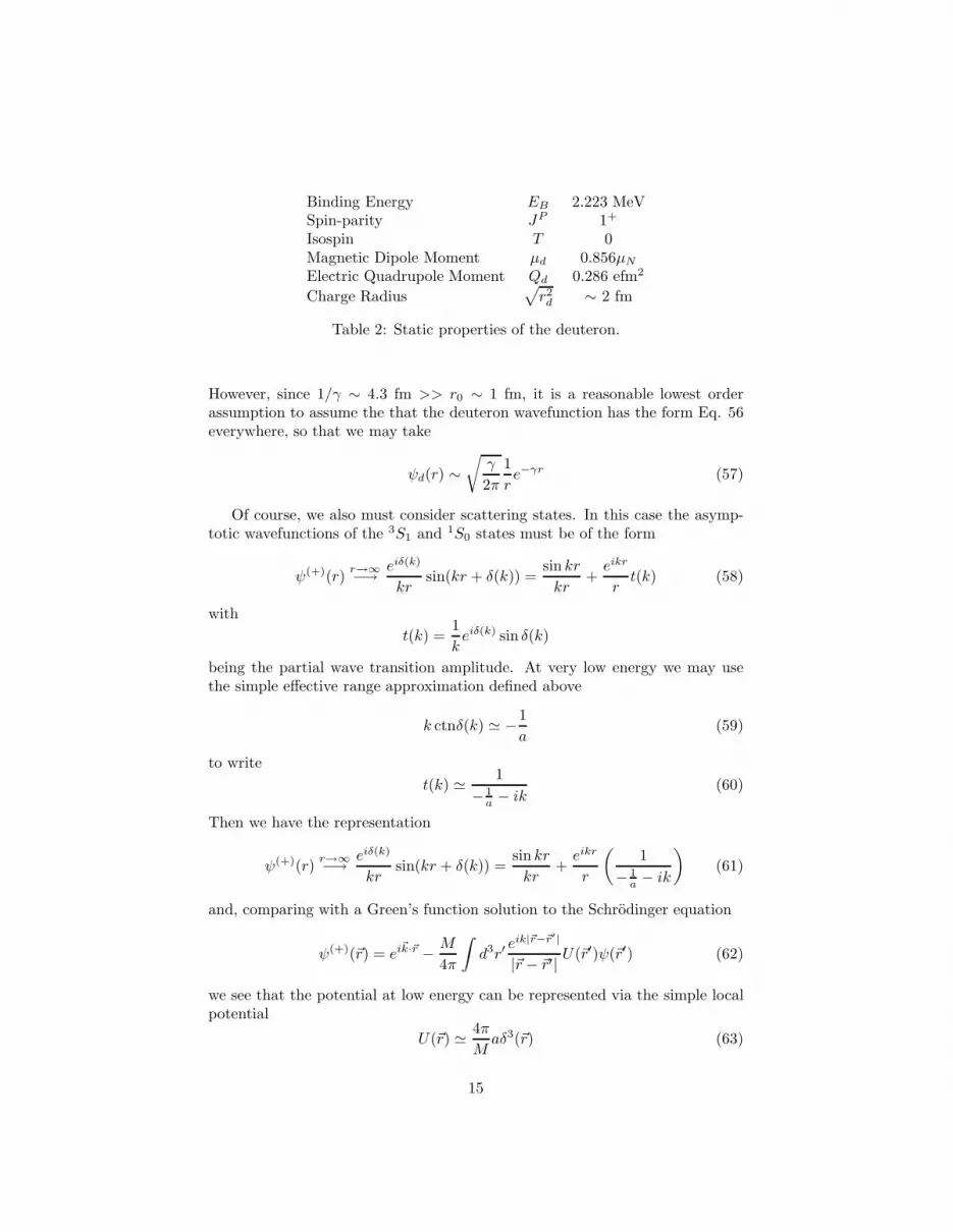
Table 2: Static properties of the deuteron.

However, since 1/γ ∼ 4.3 fm >> r0 ∼ 1 fm, it is a reasonable lowest orderassumption to assume the that the deuteron wavefunction has the form Eq. 56everywhere, so that we may take

ψd(r) ∼√

γ

2π

1

re−γr (57)

Of course, we also must consider scattering states. In this case the asymp-totic wavefunctions of the 3S1 and 1S0 states must be of the form

ψ(+)(r)r→∞−→ eiδ(k)

krsin(kr + δ(k)) =

sin kr

kr+eikr

rt(k) (58)

with

t(k) =1

keiδ(k) sin δ(k)

being the partial wave transition amplitude. At very low energy we may usethe simple effective range approximation defined above

k ctnδ(k) ≃ −1

a(59)

to write

t(k) ≃ 1

− 1a− ik

(60)

Then we have the representation

ψ(+)(r)r→∞−→ eiδ(k)

krsin(kr + δ(k)) =

sin kr

kr+eikr

r

(

1

− 1a− ik

)

(61)

and, comparing with a Green’s function solution to the Schrodinger equation

ψ(+)(~r) = ei~k·~r − M

4π

∫

d3r′eik|~r−~r′|

|~r − ~r′| U(~r′)ψ(~r′) (62)

we see that the potential at low energy can be represented via the simple localpotential

U(~r) ≃ 4π

Maδ3(~r) (63)

15

which is sometimes called the zero-range approximation (ZRA) and is equivalentto the contact potential used in the EFT approach.

The relation between the scattering and bound state descriptions can be ob-tained by using the feature that the deuteron wavefunction must be orthogonalto its 3S1 counterpart. This condition reads

0 =

∫

d3rψ†d(r)ψt(r) =

√

8πγ

∫ ∞

0

dre−γr

(

1

ksin kr + eikrtt(k)

)

=√

8πγ

(

1

γ2 + k2+

1

γ − iktt(k)

)

=

√8πγ

γ − ik

(

1

γ + ik+

1

− 1at

− ik

)

(64)

which requires that γ = 1/at. This necessity is also clear from the alreadymentioned feature that the deuteron represents a pole in tt(k) in the limit ask → iγ—i.e., −1/at+γ = 0. Since 1

γ∼ 4.3 fm, this equality holds to within 20%

or so and indicates the precision of our approximation. In spite of this roughness,there is much which can be learned from this simple analytic approach.

We begin with the charge radius, which is defined via

< r2d >=< r2p > +

∫

d3r1

4r2|ψd(r)|2 (65)

Note here that we have included the finite size of the proton, since it is compa-rable to the deuteron size and have scaled the wavefunction contribution by afactor of four since ~rp = 1

2~r. Performing the integration, we have

∫

d3r1

4r2|ψd(r)|2 = π

∫ ∞

0

drr2u2(r) =1

8γ2(66)

and, since < r2p >≃ 0.65 fm2 we find

√

< r2d > =

√

0.65 +1

8γ2fm ≃ 1.8 fm (67)

which is about 10% too low and again indicates the roughness of our approxi-mation.

Now consider the magnetic moment, for which the relevant operator is

~M =e

2M(µp~σp + µn~σn) +

e

2M~Lp

=e

4M

(

~J + µV (~σp − ~σn) + (µS − 1

2)(~σp + ~σn)

)

(68)

where ~J = ~L+ 12 (~σp +~σn) is the total angular momentum, µV = µp−µn = 4.70,

µS = µp+µn = 0.88 are the isovector, isoscalar moments, and the “extra” factorof 1/2 associated with the orbital angular momentum comes from the obvious

identity ~Lp = ~L/2. We find then

e

2Mµd = < ψd; 1, 1|M3|ψd; 1, 1 >=

e

4M[1 + (2µS − 1) < ψd; 1, 1|S3|ψd; 1, 1 >]

16

=e

4M

[

1 + (2µS − 1)

∫

d3r(u2d(r) +

9

8w2(r)

(

(cos2 θ − 1

3)2 − sin4 θ

)]

=e

2M

[

µS − 3

2(µS − 1

2)

∫ ∞

0

drw2d(r)

]

(69)

In the lowest order approximation—neglecting the D-wave component of thedeuteron—we find

< 1, 1|M3|1, 1 >≃ µS

e

2M(70)

and this prediction—µd = µS = 0.88µN—is in good agreement with the exper-imental value µexp

d = 0.856µN .

4.1 D-Wave Effects

A second static observable is the quadrupole moment Qd, which is a measureof deuteron oblateness. In this case a pure S-wave picture predicts a sphericalshape so that Qd = 0. Thus, in order to generate a quadrupole moment, wemust introduce a D-wave piece of the wavefunction. Now, just as we related theℓ = 0 wavefunction to the np scattering in the spin triplet state, we can relatethe D-wave component to the scattering amplitude provided we include spin.Thus, if we write the general scattering matrix consistent with time reversal andparity-conservation as[43]

M(~k′, ~k) = α+ β~σp · n~σn · n+ ρ(~σp + ~σn) · n+ (κ+ λ)~σp · n+~σn · n− + (κ− λ)~σp · n−~σn · n+ (71)

where

n± =~k ± ~k′

|~k ± ~k′|, n =

~k × ~k′

|~k × ~k′|,

we can represent the asymptotic scattering wavefunction via

ψ(r)r→∞−→ ei~k·~r + M(−i~∇, ~k)

eikr

r(72)

A useful alternative form for M can be found via the identity

~σp · n~σn · n = ~σp · ~σn − ~σp · n+~σn · n+ − ~σp · n−~σn · n− (73)

and, using the deuteron spin vector ~S = 12 (~σp + ~σn), it is easy to see that

M(~k′, ~k) = −at+1

M2

[

c′~S · ~k × ~k′ + g1(~S · (~k + ~k′))2 + g2(~S · (~k − ~k′))2]

(74)

where

c′ =2ρM2

k2 sin θ, g1 =

(κ− β + λ)M2

2k2 cos2 θ2

, g2 =(κ− β − λ)M2

2k2 sin2 θ2

17

Then, since in the ZRA

~k′ → −i~∇δ3(~r), ~k → δ3(~r) · −i~∇ (75)

we find the effective local potential

U(~r) =4π

M

[

atδ3(~r) +

c′

M2ǫijkSi∇jδ

3(~r)∇k

+1

2M2Sij

(

(g1 + g2)∇i∇j , δ3(~r) + (g1 − g2)(∇iδ

3(~r)∇j + ∇jδ3(~r)∇i)

)

]

(76)

where

Sij = SiSj + SjSi −4

3δij (77)

Using the Green’s function representation—Eq. 72, the asymptotic form of thetriplet scattering wavefunction becomes

ψ(r)r→∞−→ ei~k·~r −

(

at +g1 + g22M2

Sij∇i∇j

)

eikr

rχt (78)

and, by continuing to the value k → iγ, we can represent the deuteron wave-function as

ψd(r) ∼√

γ

2π

(

1 +g1 + g22M2at

Sij∇i∇j

)

1

re−γrχt (79)

A little work shows that this can be written in the equivalent form

ψd(r) ∼√

γ

2π

[

1 +g1 + g22M2at

Opn

(

d2

dr2− 1

r

d

dr

)]

1

re−γrχt

=

√

γ

2π

[

1 +g1 + g22M2at

Opn

(

3

r2+

3γ

r+ γ2

)]

1

re−γrχt (80)

Here the asymptotic ratio of S- and D-wave amplitudes is an observable and isdenoted by

η =AD

AS

=

√2(g1 + g2)

3M2a3t

(81)

This quantity has been determined experimentally from elastic dp scatteringand from neutron stripping reactions to be[44]

η = 0.0271 ± 0.0004, i.e., g1 + g2 = 105 fm

Defining the quadrupole operator1

Qij ≡ e

4(3rirj − δijr

2)

1Note that the factor of 1

4arises from the identity ~r2

p = 1

4~r2

18

and using∫

dΩ

4πrirj rk rℓ =

1

15(δijδkℓ + δiℓδjk + δikδjℓ) (82)

we note∫

d3rψ∗d(~r)Qijψd(~r) ≃ 2e

∫

d3rχ†t

1

ru(r)Qij

(g1 + g2)γ

2M2Opn

(

3

r3+

3γ

r2+γ2

r

)

u(r)χt

=3e

2· 1

15

g1 + g2)γ

2M2

γ

2πχ†

t

(

σpiσnj + σpjσni −2

3δij~σp · ~σn

)

χt

× 4π

∫ ∞

0

dre−2γr(3 + 3γr + γ2r2)

=1

5

e(g1 + g2)γ2

2M2χ†

t

(

σpiσnj + σpjσni −2

3δij~σp · ~σn

)

χt

(

3

2γ+

3γ

(2γ)2+

2γ2

(2γ)3

)

=e(g1 + g2)γ

4M2χ†

t

(

σpiσnj + σpjσni −2

3δij~σp · ~σn

)

χt (83)

Then the quadrupole moment is found to be

Qthd =< ψd; 1, 1|Qzz|ψd; 1, 1 >=

e(g1 + g2)

3atM2≃ 0.28 e fm2, (84)

in good agreement with the experimental value

Qexpd = 0.286 e fm2

From its definition, we observe that the quadrupole moment would vanish for aspherical (purely S-wave) deuteron and that a positive value indicates a slightelongation along the spin axis.

Note that in interpreting the meaning of the D-wave piece of the deuteronwavefunction one often sees things described in terms of the D-state probability

PD =

∫ ∞

0

drw2(r)

However, since∫

d3r(3

r2+

3γ

r+ γ2)2 exp(−2γr) (85)

diverges while in reality the D-wave function wd(r) must vanish as r → 0, it isclear that the connection between the asymptotic amplitude η and the D-stateprobability PD must be model dependent. Nevertheless, the D-state piece is asmall but important component of the deuteron wavefunction. As one indicationof this, let’s return to the magnetic moment calculation and insert the D-wavecontribution. We find then

µd = µS − 3

2(µS − 1

2)PD (86)

19

If we insert the experimental value µd = 0.857 we find PD ≃ 0.04 which cannow be used in other venues. However, it should be kept in mind that thisanalysis is only approximate, since we have neglected relativisitic corrections,meson exchange currents, etc.

Of course, static properties represent only one type of probe of deuteronstructure. Another is provided by the use of electromagnetic interactions,for which a well-studied case is photodisintegration—γd → np—or radiativecapture—np→ dγ—which are related by time reversal invariance.

5 Parity Conserving Electromagnetic Interaction:

np ↔ dγ

An important low energy probe of deuteron structure can be found within theelectromagnetic transtion np ↔ dγ. Here the np scattering states include bothspin-singlet and -triplet components and we must include a bound state—thedeuteron. For simplicity, we represent the latter by purely the dominant S-wavecomponent, which has the form

ψd(r) =

√

γ

2π

1

re−γr, or ψd(q) =

√8πγ

γ2 + q2(87)

Since we are considering an electromagnetic transition at very low energy wecan be content to include only the lowest—E1, M1, and E2—mutipoles, whichare described by the Hamiltonian[42]

H = es0ǫγ ·[

±i12~r +

1

4Msγ ×

(

µV (~σp − ~σn) + (µS − 1

2)(~σp + ~σs)

)

− i

8~r~r · ~k

]

(88)Here ~sγ is the photon momentum, µV , µS = µp ±µn are the isoscalar, isovectormagnetic moments, and we have used Siegert’s theorem to convert the conven-tional ~p · ~A/M interaction into the E1 form given above.2 The ± in front of theE1 operator depends upon whether the np → dγ or γd → np reaction is underconsideration. The electromagnetic transition amplitude then can be written inthe form

Amp = χ†f [ǫγ × sγ · (GM1V (~σp − ~σn) +GM1S(~σp + ~σn))

+ GE1ǫγ · k +GE2 (~σp · ǫγ~σn · sγ + ~σn · ǫγ~σp · sγ)]

χi (89)

The leading parity-conserving transition at near-threshold energy is then theisovector M1 amplitude—GM1V —which connects the 3S1 deuteron to the 1S0

scattering state of the np system. From Eq. 88 we identify

GM1V =es0µV

4M

∫

d3rψ(−)∗1S0

(kr)ψd(r) (90)

2Note that the factor of two (eight) in the E1 (E2) component arises from the obviousidentity ~rp →

1

2~r[43].

20

Using the asymptotic form

ψ(−)1S0

(kr) =e−iδs

kr(sin kr cos δs + cos kr sin δs) (91)

the radial integral becomes

∫

d3rψ(−)∗1S0

(kr)ψd(r) =4πeiδs

k

∫ ∞

0

(sin kr cos δs + cos kr sin δs)e−γr

=4πeiδs

k(k2 + γ2)(k cos δs + γ sin δs) (92)

Since by energy conservation

s0 =k2 + γ2

M

we can use the lowest order effective range values for the scattering phase shiftto this result in the form

GM1V =eµV

√8πγe−itan−1kas(1 − γas)

4M2√

1 + k2a2s

(93)

Note here that the phase of the amplitude is required by the Fermi-Watsontheorem, which follows from unitarity.

The M1 cross section is then found by squaring and mutiplying by phasespace. In the case of radiative capture this is found to be

Γnp→dγ =1

|~vrel|

∫

d3s

(2π)32s02πδ(s0 −

γ2

M− k2

M)∑

λγ

1

4TrPtTT

† (94)

Here

∑

λγ

1

4TrPtTT

† =|GM1V |2

4Tr

1

4(3 + ~σ1 · ~σ2)ǫ∗γ × sγ · (~σp − ~σn)ǫγ × sγ · (~σp − ~σn)

=∑

λγ

|GM1V |2ǫ∗γ × sγ · ǫγ × sγ = 2|GM1V |2 (95)

yielding

σM1(np→ dγ) =s0

2π|~vrel|2|GM1V |2 =

2παµ2V γ(1 − γas)2(k2 + γ2)

M5(1 + k2a2s)

(96)

Putting in numbers we find that for an incident thermal neutrons with relativevelocity |~vrel| = 2200 m/sec. the predicted cross section is about 300 mb whichis about 10% smaller than the experimental value

σexp = 334 ± 0.1 mb

21

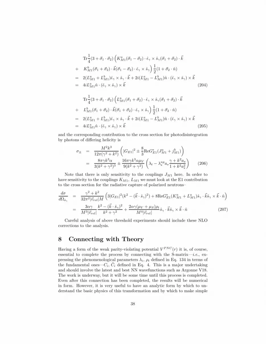
(a) (b)

...

(c)

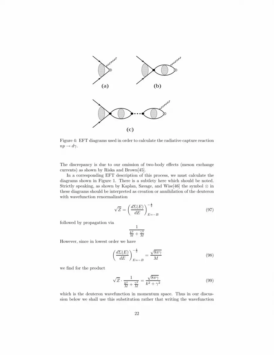
Figure 4: EFT diagrams used in order to calculate the radiative capture reactionnp→ dγ.

The discrepancy is due to our omission of two-body effects (meson exchangecurrents) as shown by Riska and Brown[45].

In a corresponding EFT description of this process, we must calculate thediagrams shown in Figure 1. There is a subtlety here which should be noted.Strictly speaking, as shown by Kaplan, Savage, and Wise[46] the symbol ⊗ inthese diagrams should be interpreted as creation or annihilation of the deuteronwith wavefunction renormalization

√Z =

(

dΣ(E)

dE

)− 1

2

E=−B

(97)

followed by propagation via1

k2

M+ γ2

M

However, since in lowest order we have

(

dΣ(E)

dE

)− 1

2

E=−B

=

√8πγ

M(98)

we find for the product

√Z · 1

k2

M+ γ2

M

=

√8πγ

k2 + γ2(99)

which is the deuteron wavefunction in momentum space. Thus in our discus-sion below we shall use this substitution rather that writing the wavefunction

22

normalization times propagator product. From Figure 4a then we find

GaM1V =

es0µV

4M

∫

d3q

(2π)3ψ

(0)∗~k

(~q)ψd(~q) (100)

Since ψ(0)∗~k

(~q) = (2π)3δ3(~k − ~q) we have

GaM1V =

es0µV

4M

√8πγ

γ2 + k2(101)

On the other hand from Figures 4b+c we find

Gb+cM1V =

es0µV

4M

(

C0s

1 − C0sG0(k)

)∗ ∫d3q

(2π)3G0(~r = 0, ~q)ψd(q) (102)

Since

G0(~r = 0, ~q) =1

k2

M− q2

M+ iǫ

(103)

this becomes

Gb+cM1V =

es0µV

4M

(

C0s

1 − C0sG0(k)

)∗ ∫d3q

(2π)3

√8πγ

(q2 + γ2)(k2

M− q2

M+ iǫ)

=es0µV

4M

(

C0s

1 − C0sG0(k)

)∗ √8πγ

γ2 + k2(G0(k) −G0(iγ))

=es0µV

4M

(

C0s

1 − C0sG0(k)

)∗ √8πγ

γ2 + k2

M

4π(−ik − γ) (104)

Adding the two contributions we have

GM1V =es0µV

4M

√8πγ

γ2 + k2

[

1 −(

−γ − ik−1as

− ik

)]

=es0µV

4M

√8πγ

γ2 + k2

(

1 − γas

1 + ikas

)

(105)

which agrees completely with Eq. 93 obtained via conventional coordinate spaceprocedures. Of course, we still have a ∼ 10% discrepancy with the experimentalcross section, which is handled by inclusion of a four-nucleon M1 countertermconnecting 3S1 and 1S0 states—

LEM2 = eLM1V

1 (NT ~P · ~BN)†(NTP3N) (106)

where here the Pi represent relvant projection operators[47].As the energy increases above threshold, it is necessary to include the cor-

responding P-conserving E1 multipole—

Amp = GE1ǫγ · ~kχ†tχt (107)

23

In this case the matrix element involves the np 3P-wave final state and, neglect-ing final state interactions in this channel, the matrix element is given by

GE1~k =

es02

∫

d3rψ(0)∗~k

(r)~rψd(r) (108)

The radial integral can be found via

− i~k ·∫

d3re−i~k·~r~rψd(r) =d

dλ |λ=1

√

γ

2π

∫

d3re−i~k·~rλ 1

re−γr

=d

dλ |λ=1

√8πγ

γ2 + k2λ2=

−2k2√

8πγ

(k2 + γ2)2(109)

Equivalently using EFT methods we have

∫

d3q

(2π)3ψ

(0)∗~k

(~q)~∇~qψd(q) =−2i

√8πγ~k

(k2 + γ2)2(110)

In either case

GE1 =−ies0

√8πγ

(k2 + γ2)2(111)

and the corresponding cross section is

σE1(np→ dγ) =1

4

3s02π|~vrel|

∫

dΩs

4π(~k · ~k − (~k · s)2)

e28πγs20(k2 + γ2)4

=8παk2γ

|~vrel|M3(k2 + γ2)(112)

It is important to note that we can easily find the corresponding photodis-integration cross sections by multiplying by the appropriate phase space. Forunpolarized photons we have

σ(γd→ np) =1

3 · 2

1

2s0

∫

d3k

(2π)3

∑

λγ

2πδ(s0 −γ2

M− k2

M)|Amp|2

=Mk

24πs0

∑

λγ

∫

dΩk

4π|Amp|2 (113)

Using the results obtained above for radiative capture—

∑

λγ

|Amp|2 = 8|GM1V |2 + 3(~k · ~k − (~k · s)2)|GE1|2 (114)

we find the photodisintegration cross sections to be

σM1(γd→ np) =2πα

3M2

(1 − asγ)2µ2V kγ

(k2 + γ2)(1 + k2a20), σE1(γd→ np) =

8παγk3

3(k2 + γ2)3

(115)

24

Although the leading electromagnetic physics is controlled, as we have seen,by the isovector M1 and E1 amplitudes, there exist small but measurableisoscalar M1 and E2 transitions[48],[49],[50]. In the former case the transition isbetween the S-wave (D-wave) deuteron ground state and into the 3S1(3D) scat-tering state. The amplitude GM1S is small because of the smallness of µS − 1

2and because of the orthogonality restriction. In the case of GE2, the resultis suppressed by the requirement for transfer of two units of angular momen-tum, so that the transition must be between S- and D-wave components of thewavefunction.

We first evaluate the isoscalar M1 amplitude, which from Eq. 88 is given by(cf. Eq. 69)

GM1S =e

2M(µS − 1

2) < ψd; 1, 1|S3|ψd, 1, 1 >

=e

2M(µS − 1

2)

∫ ∞

0

dr(ud(r)ut(r) −1

2wd(r)wt(r))

= − e

2M(µS − 1

2)3

2

∫ ∞

0

drwt(r)wd(r) (116)

where the last form was fouind using the orthogonality condition. In orderto estimate the latter, we follow Danilov in assuming that, since the radialintegral is short-distance dominated, the D-wave deuteron and scattering piecesare related by a simple constant[51], which, using orthogonality, must be givenby

wt(r) ≃ −at

√

2π

γwd(r) (117)

The matrix element then becomes

GM1S ≃ e

2M(µS − 1

2)3

2PDat (118)

Likewise, using Eq. 82 we note that∫

d3r

(

1

rut(r) +

3√8Opn

1

rwt(r)

)

~r · ǫγ~r · sγψd(~r)

=3√8

1

15

∫ ∞

0

drr2(ut(r)wd(r) + wt(r)ud(r)) [~σp · ǫγ~σn · sγ + ~σn · ǫγ~σp · sγ ]

(119)

so that the corresponding E2 coupling is found to be

GE2 =es0

80√

2

∫ ∞

0

drr2(ut(r)wd(r) + wt(r)ud(r)) = − es0

80√

2

g1 + g22M2

(120)

In order to detect these small components we can use the circular polariza-tion induced in the final state photon by an initially polarized neturon, whichis found to be

Pγ = −2

(

GM1S −GE2

GM1V

)

(121)

25

Putting in numbers we find

Pγ = Pγ(M1) + Pγ(E2)

=−γat

µV (1 − γas)

(

µS − µd +2

15

γ2(g1 + g2)

atM2

)

≃ −1.17 × 10−3 − 0.24 × 10−3

= −1.41 × 10−3 (122)

which is in reasonable agreement with the experimental value[52]

P expγ = (−1.5 ± 0.3) × 10−3 (123)

Having familiarized ourselves with the analytic techniques which are needed,we now move to our main subject, which is hadronic parity violation in the NNsystem.

6 Parity-Violating NN Scattering

For simplicity we begin again with a system of two nucleons. Then the NNscattering-matrix can be written at low energies in the phenomenological form[51]

M(~k′, ~k) = mt(k)P1 +ms(k)P0 (124)

where

P1 =1

4(3 + ~σ1 · ~σ2), P0 =

1

4(1 − ~σ1 · ~σ2)

are spin-triplet, -singlet spin projection operators and

mt(k) =−at

1 + ikat

, ms(k) =−as

1 + ikas

(125)

are the S-wave partial wave amplitudes in the lowest order effective range ap-proximation, keeping only the scattering lengths at, as. Here the scattering crosssection is found via

dσ

dΩ= TrM†M (126)

so that at the lowest energy we have the familiar form

dσs,t

dΩ=

|as,t|21 + k2a2

s,t

(127)

The corresponding scattering wavefunctions are then given by

ψ(+)~k

(~r) =

[

ei~k·~r − M

4π

∫

d3r′eik|~r−~r′|

|~r − ~r′| U(~r′)ψ(+)~k

(~r)

]

χ

r→∞−→[

ei~k·~r + M(−i~∇, ~k)eikr

r

]

χ (128)

26

where χ is the spin function. In Born approximation we can represent thewavefunction in terms of an effective delta function potential

Ut,s(~r) =4π

M(atP1 + asP0)δ3(~r) (129)

as can be confirmed by substitution into Eq. 128.

6.1 Including the PV Interaction

Following Danilov,[51], we can introduce parity mixing into this simple represen-tation by generalizing the scattering amplitude to include P-violating structures.Up to laboratory energies of 50 MeV or so, we can omit all but S- and P-wavemixing, in which case there exist only five independent such amplitudes:

i) dt(k) representing 3S1 −−1P1 mixing;

ii) d0,1,2s (k) representing 1S0 −−3P0 mixing with ∆I = 0, 1, 2 respectively;

iii) ct(k) representing 3S1 −−3P1 mixing.

After a little thought, it becomes clear then that the low energy scattering-matrix in the presence of parity violation can be written as

M(~k′, ~k) =

[

ms(k)P0 + ct(k)(~σ1 + ~σ2) · (~k′ + ~k)1

2(τ1 − τ2)z

+ (~σ1 − ~σ2) · (~k′ + ~k)

(

P0d0s(k) +

1

2(τ1 + τ2)zd

1s(k) +

3τ1zτ2z − ~τ1 · ~τ22√

6d2

s(k)

)]

+[

mt(k) + dt(k)(~σ1 − ~σ2) · (~k′ + ~k)]

P1 (130)

Note that since under spatial inversion—~σ → ~σ,~k,~k′ → −~k,−~k′—each of thenew pieces is P-odd, and since under time reversal—~σ → −~σ,~k,~k′ → −~k′,−~kthe terms are each T-even. At very low energies the coefficients in the T-matrixbecome real and we define[51]

limk→0

ms,t(k) = as,t, limk→0

ct(k), ds(k), dt(k) = ρtat, λisas, λtat (131)

(The reason for factoring out the S-wave scattering length will be describedpresently.) The five real numbers ρt, λ

is, λt then completely characterize the low

energy parity-violating interaction and can in principle be determined experi-mentally, as we shall discuss below.3 Alternatively, we can write things in termsof the equivalent notation

λpps = λ0

s + λ1s +

1√6λ2

s

3Note that there exists no singlet analog to the spin-triplet constant ct since the combina-tion ~σ1 + ~σ2 is proportional to the total spin operator and vanishes when operating on a spinsinglet state.

27

λnps = λ0

s −2√6λ2

s

λnns = λ0

s − λ1s +

1√6λ2

s (132)

We can also represent this interaction in terms of a simple effective NNpotential. Integrating by parts, we have

∫

d3r′eik|~r−~r′|

|~r − ~r′| −i~∇, δ3(~r′)ei~k·~r′

= (−i~∇ + ~k)eikr

r(133)

which represents the parity-violating admixture to the the scattering wavefunc-

tion in terms of an S-wave admixture to the scattering P-wave state—∼ ~σ ·~k eikr

r

plus a P-wave admixture the scattering S-state—∼ −i~σ · ~∇ eikr

r. We see then

that the scattering wave function can be described via

U(~r) =4π

M

[(

atδ3(~r) + λtat(~σ1 − ~σ2) · −i~∇, δ3(~r)

)

P1

+ asδ3(~r)P0 + ρtat(~σ1 + ~σ2) · −i~∇, δ3(~r)1

2(τ1 − τ2)z

+ (~σ1 − ~σ2) · −i~∇, δ3(~r)as

(

P0λ0s +

1

2(τ1 + τ2)zλ

1s +

3τ1zτ2z − ~τ1 · ~τ22√

6λ2

s

)]

(134)

However, before application of this effective potential we must worry about thestricture of unitarity, which requires that

2ImT = T †T (135)

In the case of the S-wave partial wave amplitude mt(k) this condition reads

Immt(k) = k|mt(k)|2 (136)

and requires the form

mt(k) =1

keiδt(k) sin δt(k) (137)

Since at zero energy we have

limk→0

mt(k) = −at (138)

It is clear that unitarity can be enforced by modifying this lowest order resultvia

mt(k) =−at

1 + ikat

(139)

which is the lowest order effective range result. Equivalently, this can easily bederived in an effective field theory (EFT) formalism. In this case the lowestorder contact interaction

T0t = C0t(µ) (140)

28

becomes, when summed to all orders in the scattering series,

Tt(k) =C0t(µ)

1 − C0t(µ)G0(k)= −M

4π

1

− 4πMC0t(µ) − µ− ik

(141)

Identifying the scattering length via

− 1

at

= − 4π

MC0t(µ)− µ (142)

and noting the relation mt(k) = −M4πTt(k) connecting the scattering and tran-

sition matrices, we see that Eqs. 139 and 141 are identical.So far, so good. However, things become more interesting in the case of the

parity-violating transitions. In this case the requirement of unitarity reads, e.g.,for the case of scattering in the 3S1 channel

Im dt(k) = k(m∗t (k)dt(k) + d∗t (k)mp(k)) (143)

where mp(k) is the 1P1 analog of the mt(k). Eq. 143 is satisfied by the solution

dt(k) = |dt(k)|ei(δ3S1(k)+δ1P1

(k)) (144)

i.e., the phase of the amplitude should be the sum of the strong interactionphases in the incoming and outgoing channels[63]. At very low energy we canneglect P-wave scattering, and can write

ct(k) ≃ ρtmt(k), dis(k) ≃ λi

sms(k), dt(k) ≃ λtmt(k) (145)

This result is also easily seen in the language of EFT, wherein the full transi-tion matrix must include the weak amplitude to lowest order accompanied byrescattering in both incoming and outgoing channels to all orders in the stronginteraction. If we represent the lowest order weak contact interaction as

T0tp(k) = D0tp(µ)(~σ1 − ~σ2) · (~k + ~k′) (146)

then the full amplitude is given by

Ttp(k) =D0tp(µ)

(1 − C0t(µ)G0(k))(1 − C0p(µ)G1(k))(~σ1 − ~σ2) · (~k + ~k′) (147)

where we have introduced a lowest order contact term C0p which describes the1P1-wave nn interaction. Since the phase of the combination 1 − C0(µ)G0(k)is simply the negative of the strong interaction phase the unitarity stricture isclear, and we can define the physical transition amplitude Atp via

D0tp(µ)

(1 − C0t(µ)G0(k))(1 − C0p(µ)G1(k))≡ Atp

(1 + ikat)(1 + ik3ap)(148)

Making the identification λt = −M4πAtp and noting that

1

1 + ikat

= cos δt(k)eiδt(k)

29

then λt is seen to be identical to the R-matrix element defined by Miller andDriscoll[63].

Now that we have developed a fully unitary transition amplitude we cancalculate observables. For simplicity we begin with nn scattering. In this casethe Pauli principle demands that the initial state must be purely 1S0 at lowenergy. One can imagine longitudinally polarizing one of the neutrons andmeasuring the total scattering cross section on an unpolarized target. Since~σ · ~k is odd under parity, the cross section can depend on the helicity only ifparity is violated. Using trace techniques the helicity correlated cross sectioncan easily be found. Since the initial state must be in a spin singlet we have

σ± =

∫

dΩ1

2TrM(~k′, ~k)

1

2(1 + ~σ2 · k)

1

4(1 − ~σ1 · ~σ2)M†(~k′, ~k)

= |ms(k)|2 ± 4kRem∗s(k)dnn

s (k) + O(d2s) (149)

Defining the asymmetry via the sum and difference of such helicity cross sectionsand neglecting the tiny P-wave scattering, we have then

A =σ+ − σ−σ+ + σ−

=8kRem∗

s(k)dnns (k)

2|ms(k)|2 = 4kλnns (150)

Thus the helicity correlated nn-scattering asymmetry provides a direct measureof the parity-violating parameter λnn

s . Note that in the theoretical evaluation ofthe asymmetry, since the total cross section is involved some investigators optto utilize the optical theorem via[64],[65]

A =4kIm dnn

s (k)

Imms(k)(151)

which, using our unitarized forms, is completely equivalent to Eq. 150.Of course, nn-scattering is purely a gedanken experiment and we have dis-

cussed it only as a warmup to the real problem—pp scattering, which introducesthe complications associated with the Coulomb interaction. In spite of this com-plication, the calculation proceeds quite in parallel to the discussion above withobvious modifications. Specifically, as shown in [66] the unitarized the scatteringamplitude now has the form

ms(k) = −M4π

C0sC2η (η+(k)) exp 2iσ0

1 − C0sGC(k)(152)

where η+(k) = Mα/2k and

C2(x) =2πx

e2πx − 1(153)

is the usual Sommerfeld factor and σ0 = argΓ(ℓ + 1 + iη(k)) is the Coulombphase shift. Of course, the free Green’s function G0(k) has also been replacedby its Coulomb analog

GC(k) =

∫

d3s

(2π)3C2(η+(k))

k2

M− s2

M+ iǫ

(154)

30

Remarkably this integral can be performed analytically and the result is

GC(k) = −M4π

[

µ+Mα(

H(iη+(k)) − logµ

πMα− ζ)]

(155)

Here ζ is defined in terms of the Euler constant γE via ζ = 2π − γE and

H(x) = ψ(x) +1

2x− log x (156)

The resultant scattering amplitude has the form

ms(k) =C2

η (η+(k))e2iσ0

− 4πMC0s

− µ−Mα[

H(iη+(k)) − log µπMα

− ζ]

=C2

η(η+(k))e2iσ0

− 1a0s

−Mα[

h(η+(k)) − log µπMα

− ζ]

− ikC2η(η+(k))

(157)

where we have defined

− 1

a0s

= − 4π

MC0s

− µ, and h(η+(k)) = ReH(iη+(k)) (158)

The experimental scattering length aCs in the presence of the Coulomb inter-action is defined via

− 1

aCs

= − 1

a0s

+Mα(

logµ

πMα− ζ)

(159)

in which case the scattering amplitude takes its traditional form

ms(k) =C2

η(η+(k))e2iσ0

− 1aCs

−MαH(iη+(k))(160)

Of course, this means that the Coulomb-corrected scattering length is differentfrom its non-Coulomb analog, and comparison of the experimental pp scatteringlength—app = −7.82 fm—with its nn analog—ann = −18.8 fm—is roughlyconsistent with Eq. 159 if a reasonable cutoff, say µ ∼ 1GeV is chosen. Havingunitarized the strong scattering amplitude, we can proceed similarly for itsparity-violating analog. Again summing the rescattering bubbles and neglectingthe small p-wave scattering, we find for the unitarized weak amplitude

T0SP =D0sp(µ)C2

η (η+(k))ei(σ0+σ1)

1 − C0s(µ)GC(k)≡ACspC

2η (η+(k))ei(σ0+σ1)

− 1aCs

−MαH(iη+(k))(161)

Here again, the Driscoll-Miller procedure identifies ACsp = λpps via the R-matrix.

Having obtained fully unitarized forms, we can then proceed to evaluate thehelicity correlated cross sections, finding as before

Ah =σ+ − σ−σ+ + σ−

=8kRem∗

s(k)dpps (k)

2|ms(k)|2 ≃ 4kλpps (162)

31

Note here that the superscript pp has been added, in order account for thefeature that in the presence of Coulomb interactions the parity mixing parameterλs which is appropriate for neutral scattering is modified, in much the same wayas the scattering length in the pp channel is modified (cf. Eq. 159). On theexperimental side such asymmetries have been measured both at low energy(13.6 and 45 MeV) as well as at higher energy (221 and 800 MeV) but it is onlythe low energy results4

Ah(13.6 MeV) = −(0.93 ± 0.20 ± 0.05) × 10−7[67]

Ah(45 MeV) = −(1.57 ± 0.23) × 10−7[68] (164)

which are appropriate for our analysis. Note that one consistency check on theseresults is that if the simple discussion given above is correct the two numbersshould be approximately related by the kinematic factor5

Ah(45 MeV)/Ah(13.6 MeV) ≃ k1/k2 = 1.8 (165)

and the quoted numbers are quite consistent with this requirement. We canthen extract the experimental number for the singlet mixing parameter as

λpps =

Ah

4k= −(4.0 ± 0.8) × 10−8 fm (166)

In principle one could extract the triplet parameters by a careful nd scatteringmeasurement. However, extraction of the neeeded np amplitude involves a de-tailed theoretical analysis which has yet not been performed. Thus instead wediscuss the case of electromagnetic interactions and consider np↔ dγ.

7 Parity Violating Electromagnetic Interaction:

np ↔ dγ

A second important low energy probe of hadronic parity violation can be foundwithin the electromagnetic transtion np ↔ dγ. Here the np scattering statesinclude both spin-singlet and -triplet components and we must include a boundstate—the deuteron. Analysis of the corresponding parity-conserving situationhas been given previously, so we concentrate here on the parity violating situ-ation. In this case, the mixing of the scattering states has already been givenin Eq. 130 while for the deuteron the result can be found from demandingorthogonality with the 3S1 scattering state—

ψd(r) =(

1 + ρt(~σp + ~σn) · −i~∇ + λt(~σp − ~σn) · −i~∇)

√

γ

2π

1

re−γr (167)

4Note that the 13.6 MeV Bonn measurement is fully consistent with the earlier but lessprecise number

Ah = −(1.7 ± 0.8) × 10−7[69] (163)

determined at LANL.5There is an additional k-dependence arising from λs but this is small.

32

Having found λs via the pp scattering asymmetry, we now need to focus on thedetermination of the parity-violating triplet parameters ρt, λ

it. In order to do

so, we must evaluate new matrix elements. There are in general two types ofPV E1 matrix elements, which we can write as

Amp =(

HE1χ†s(~σp − ~σn)χt + SE1χ

†t (~σp + ~σn)χt

)

· ǫγ (168)

and there exist two separate contributions to each of these amplitudes, depend-ing upon whether the parity mixing occurs in the inital or final state. We beginwith the matrix element which connects the 1P1 admixture of the deuteron tothe 1S0 scattering state.

HE1(1P − 1S) =es0λt

2

1

3

∫

d3rψ(−)∗1S

(r)~r · ~∇ψd(r)

=es04πλt

6eiδs

∫ ∞

0

drr21

kr(sin kr cos δs + cos kr sin δs)~r · ~∇

√

γ

2π

1

re−γr

=es0

√8πγλt

6

eiδs

k

× (1 − γd

dγ)

∫ ∞

0

dr(sin kr cos δs + cos kr sin δs)e−γr

=es0λt

√8πγe−itan−1kas

6√

1 + k2a2s

×[

k2 + 3γ2

(k2 + γ2)2− γas

2γ2

(k2 + γ2)2

]

(169)

Equivalently we can use EFT methods using the diagrams of Figure 4. We havefrom Figure 4a

HaE1(1P − 1S) =

es0λt

2

1

3

∫

d3q

(2π)3ψ

(0)∗~k

(~q)~∇~q · (~qψd(q))

=es0λt

√8πγ

6

k2 + 3γ2

(k2 + γ2)2(170)

while from the bubble sum in Figure 4b+c we find

Hb+cE1 (1P − 1S) =

es0λt

2

1

3

(

C0s

1 − C0sG0(k)

)∫

d3q

(2π)3G0(~r = 0, ~q)~∇~q · (~qψd(q))

=es0M

√8πγλt

6

(

C0s

1 − C0sG0(k)

)

×∫

d3q

(2π)3q2 + 3γ2

(q2 + γ2)2(k2

M− q2

M+ iǫ)

(171)

Here the integral may be evaluated via∫

d3q

(2π)3q2 + 3γ2

(q2 + γ2)2(k2

M− q2

M+ iǫ)

= (1 − 2γ2 d

dγ2)

1

(k2 + γ2)(G0(k) −G0(iγ))

33

=1

4π

2γ − ik

(γ − ik)2(172)

Summing the two results we find

HE1(1P − 1S) =es0

√8πγλt

2

1

3(k2 + γ2)2

(

k2 + 3γ2 − as

(2γ − ik)(γ + ik)2

1 + ikas

)

=es0

√8πγλt

6

k2 + 3γ2 − 2γ3as

(k2 + γ2)2(1 + ikas)(173)

as found using coordinate space methods.The matrix element HE1 also receives contributions from the E1 amplitude

connecting the deuteron wavefunction with the 3P mixture of the final statewavefunction mixed into the 1S0. This admixture can be read off from theGreen’s function representation of the scattering amplitude as

δ3Pψ1S0= −ims(k)(~σp − ~σn) · ~∇eikr

r(174)

and leads to an E1 amplitude

HE1(3P − 3S) =es0λ

nps m∗

s(k)

2

1

3

∫

d3rψd(r)~r · ~∇e−ikr

rψ∗

1S0(kr)

− es0λnps

√8πγ

6

(

as

1 − ikas

)∫ ∞

0

dr(1 + ikr)e−(γ+ik)r

= −es0λnps

√8πγ

6

(

as

1 − ikas

)

γ + 2ik

(γ + ik)2

= −es0λnps as

√8πγe−itan−1kas

6(k2 + γ2)2√

1 + k2a2s

(γ(γ2 + 3k2) − 2ik3) (175)

Equivalently we can use EFT techniques. In this case there is no analog ofFigure 4a. For the remaining diagrams, however, we find

Hb+cE1 (3P − 3S) =

es0λnps

2

1

3

(

C0s

1 − C0sG0(k)

)

×∫

d3q

(2π)3ψd(q)~∇~q · ~qG0(~r = 0, ~q)

=es0λ

nps

√8πγ

6

(

C0s

1 − C0sG0(k)

)

×(

1 + γ2 d

dγ2

)

2

k2 + γ2(G∗

0(k) −G∗0(−iγ))

=es0λ

nps

6

(

C0s

1 − C0sG0(k)

)

M

4π

γ(γ2 + 3k2) − 2ik3

(γ2 + k2)2(176)

i.e.,

HE1(3P − 3S) = −es0λnps

√8πγe−itan−1kas

6(k2 + γ2)2√

1 + k2a2s

as[(γ2 + 3k2)γ − 2ik3] (177)

34

as found in coordinate space.The full matrix element is then found by combining the singlet and triplet

mixing contributions—

HE1 = HE1(3P − 3S) +HE1(1P − 1S)

=es0

√8πγe−iδs

6√

1 + k2a2s(k2 + γ2)2

×[

λt(k2 + 3γ2 − 2asγ

3) + λnps γas[(γ2 + 3k2)γ − 2ik3])

]

(178)

In the case of the PV E1 matrix element SE1 the calculation appears to benearly identical, except for the feature that now the spin triplet final state isinvolved, so that the calculation already performed in the case of HE1 can betaken over directly provided that we make the substitutions λnp

s , λt → ρt, as →at. The result is found then to be

SE1 =es0

√8πγe−itan−1katρt

6√

1 + k2a2t (k2 + γ2)2

[

(k2 + 3γ2 − 2atγ3) + at[γ(γ2 + 3k2) − 2ik3])

]

(179)At the level of approximation we are working we can identify at with 1/γ sothat Eq. 179 becomes

SE1 =es0

√8πγe−itan−1 k

γ ρt(γ2 + 2k2 − ik3

γ)

3√

1 + k2

γ2 (k2 + γ2)2(180)

Now consider how to detect these PV amplitudes. The parity violatingelectric dipole amplitude HE1 can be measured by looking at the circular po-larization which results from unpolarized radiative capture at threshold or bythe asymmetry resulting from the scattering of polarized photons in photodis-integration. At threshold, we have for photons of positive/negative helicity

Amp± = (±GM1V +HE1)ǫγ · χ†s(~σp − ~σn)χt + SE1ǫγ · χ†

t (~σp + ~σn)χt (181)

and the corresponding cross sections are found to be

σ±(np→ dγ) =s0

2π|~vrel|| ∓GM1V +HE1|2 + O(S2

E1) (182)

Thus the spin-conserving E1 amplitude SE1 does not interfere with the leadingM1 and the circular polarization is given by

Pγ =σ+ − σ−σ+ + σ−

= − 2HE1

GM1V

= − 4M

3µV (1 − γas)(k2 + γ2)

[

λt(k2 + 3γ2 − 2asγ

3)

+ λnps γas(γ2 + 3k2))

]

(183)

A bit of thought makes it clear that this is also the asymmetry parameterbetween right- and left-handed circularly polarized cross sections in the photo-disintegration reaction γ±d → np, and so we have the usual identity betweenpolarization and asymmetry which is guaranteed by time reversal invariance

Pγ(np→ d~γ) = Aγ(~γd→ np)

35

In order to gain sensitivity to the matrix element SE1 one must use polarizedneutrons. In this case the appropriate trace is found to be

Tr1

4(3 + ~σ1 · ~σ2)T

1

2(1 + σn · n)T † = 4|GM1V |2 + 8ReG∗

M1V SE1n · sγ (184)

In this case HE1 does not interfere with GM1V and the corresponding front-backphoton asymmetry is

Aγ =2ReG∗

M1V SE1

|GM1V |2 = − 8Mρt

3µV (1 − γas)

(

γ2 + 2k2

γ2 + k2

)

(185)

In principle then precise experiments measuring the circular polarization andphoton asymmetry in thermal neutron capture on protons can produce theremaining two low energy parity violating parameters λnp

t and ρt which weseek. At the present time only upper limits exist, however. In the case of thecircular polarization we have the number from a Gatchina measurement[70]

Pγ = (1.8 ± 1.8) × 10−7 (186)

while in the case of the asymmetry we have

Aγ = (−1.5 ± 4.7) × 10−8 (187)

from a Grenoble experiment[71]. This situation should soon change, as a newhigh precision asymmetry measurement at LANL is being run which seeks toimprove the previous precision by an order of magnitude[72].

Appendix

Of course, as we move above threshold we must also include the parity-violating M1 matrix elements, which interfere with the leading E1 amplitudeand are of two types. The first is the M1 amplitude which connects the 1P1

admixture of the deuteron with the 3P np scattering state as well as the M1amplitude connecting the 1S0 admixture of the final 3P scattering state withthe deuteron ground state. For the former we have6

Amp = JaM1χ

†t(~σ1 − ~σ2) · ǫγ × sγ(~σ1 − ~σ2) · ~kχt (188)

where

JaM1 =

es0µV

4M

λt

k2

∫

d3re−i~k·~r~k · ~∇ψd(r) =es0µV

4M

λt

√8πγ

(k2 + γ2)(189)

while for the latter we find

Amp = JbM1χ

†t(~σ1 − ~σ2) · ~k(~σ1 − ~σ2) · ǫγ × sγχt (190)

6For simplicity here we include only the dominant isovector M1 amplitude. A completediscussion should also include the corresponding isoscalar M1 transition.

36

where

JbM1 =

es0µV

4Mλnp

s m∗s(k)

∫

d3r1

re−ikrψd(r) = −es0µV

4M

λnps as

√8πγ

(1 − ikas)(γ + ik)(191)

A second category of PV M1 amplitudes involves that which connects the3P1 piece of the deuteron wavefunction with the 1P1 or 3P np scattering statesas well as the M1 amplitude connecting the 3S1 or 1S0 admixture of the final3P scattering state with the deuteron ground state. For the former we have

KaM1χ

†s[(~σ1 − ~σ2) · ǫγ × sγ(~σ1 + ~σ2) · ~kχt (192)

LaM1χ

†t [(~σ1 + ~σ2) · ǫγ × sγ(~σ1 + ~σ2) · ~kχt (193)

where

KaM1 =

es0µV

4M

ρt

k2

∫

d3re−i~k·~r~k · ~∇ψd(r) =es0µV

4M

ρt

√8πγ

k2 + γ2(194)

LaM1 =

es0µS

4M

ρt

k2

∫

d3re−i~k·~r~k · ~∇ψd(r) =es0µS

4M

ρt

√8πγ

k2 + γ2(195)

while for the latter we have

Amp = KbM1χ

†s(~σ1 + ~σ2) · ~k(~σ1 − ~σ2) · ǫγ × sγχt (196)

Amp = LbM1χ

†t(~σ1 + ~σ2) · ~k(~σ1 + ~σ2) · ǫγ × sγχt (197)

where

KbM1 =

es0µV

4Mρtm

∗t (k)

∫

d3r1

re−ikrψd(r) = −es0µV

4M

ρtat

√8πγ

(1 − ikat)(γ + ik)(198)

LbM1 =

es0µS

4Mρtm

∗t (k)

∫

d3r1

re−ikrψd(r) = −es0µS

4M

ρtat

√8πγ

(1 − ikat)(γ + ik)(199)

To this order we can use at ≃ 1/γ, so that

KbM1 = −es0µV

4M

ρt

√8πγ

k2 + γ2(200)

LbM1 = −es0µS

4M

ρt

√8πγ

k2 + γ2(201)

We see then that this piece of the M1 amplitude has the form

Amp = 2i(ǫγ × sγ) × ~k · χ†f [Ka

M1(~σ1 − ~σ2) + LaM1(~σ1 + ~σ2)]χt (202)

The relevant traces here are

Tr1

4(3 + ~σ1 · ~σ2)

(

JaM1(~σ1 − ~σ2) · ǫγ × sγ(~σ1 − ~σ2) · ~k

+ JbM1(~σ1 − ~σ2) · ~k(~σ1 − ~σ2) · ǫγ × sγ

) 1

2(1 + ~σ2 · n)

= 2(JaM1 + Jb

M1)ǫγ × sγ · ~k + 2i(JaM1 − Jb

M1)n · (ǫγ × sγ) × ~k (203)

37

Tr1

4(3 + ~σ1 · ~σ2)

(

KaM1(~σ1 − ~σ2) · ǫγ × sγ(~σ1 + ~σ2) · ~k

+ KbM1(~σ1 + ~σ2) · ~k(~σ1 − ~σ2) · ǫγ × sγ

) 1

2(1 + ~σ2 · n)

= 2(LaM1 + Lb

M1)ǫγ × sγ · ~k + 2i(LaM1 − Lb

M1)n · (ǫγ × sγ) × ~k

= 4iLaM1n · (ǫγ × sγ) × ~k (204)

Tr1

4(3 + ~σ1 · ~σ2)

(

LaM1(~σ1 + ~σ2) · ǫγ × sγ(~σ1 + ~σ2) · ~k

+ LbM1(~σ1 + ~σ2) · ~k(~σ1 + ~σ2) · ǫγ × sγ

) 1

2(1 + ~σ2 · n)

= 2(LaM1 + Lb

M1)ǫγ × sγ · ~k + 2i(LaM1 − Lb

M1)n · (ǫγ × sγ) × ~k

= 4iLaM1n · (ǫγ × sγ) × ~k (205)

and the corresponding contribution to the cross section for photodisintegrationby photons of differing helicity is

σ± =M2k3

12π(γ2 + k2)

(

|GE1|2 ±8

3ReG∗

E1(JaM1 + jb

M1)

)

=8πγk3α

3(k2 + γ2)3± 16πγk3αµV

9(k2 + γ2)

(

λt − λnps as

γ + k2as

1 + k2a2s

)

(206)

Note that there is only sensitivity to the couplings JM1 here. In order tohave sensitivity to the couplings KM1, LM1 we must look at the E1 contributionto the cross section for the radiative capture of polarized neutrons–

dσ

dΩsγ

=γ2 + k2

32π2|~vrel|M(

3|GE1|2(k2 − (~k · sγ)2) + 8ReG∗E1(Ka

M1 + LaM1)sγ · ~ksγ × ~k · n

)

=3αγ

M3|~vrel|k2 − (~k · sγ)2

k2 + γ2+

2αγ(µV + µS)ρt

M4|~vrel|sγ · ~ksγ × ~k · n (207)

Careful analysis of above threshold experiments should include these NLOcorrections to the analysis.

8 Connecting with Theory

Having a form of the weak parity-violating potential V PNC(r) it is, of course,essential to complete the process by connecting with the S-matrix—i.e., ex-pressing the phenomenological parameters λi, ρt defined in Eq. 134 in terms ofthe fundamental ones—Ci, Ci defined in Eq. 4. This is a major undertakingand should involve the latest and best NN wavefunctions such as Argonne V18.The work is underway, but it will be some time until this process is completed.Even after this connection has been completed, the results will be numericalin form. However, it is very useful to have an analytic form by which to un-derstand the basic physics of this transformation and by which to make simple

38

numerical estimates. For this purpose we shall employ simple phenomenologicalNN wavefunctions, as described below.

Examination of the scattering matrix Eq. 130 reveals that the parametersλs,t are associated with the (short-distance) component while ρt contains con-tributions from the both (long-distance) pion exchange as well as short distanceeffects. In the former case, since the interaction is short ranged we can use thisfeature in order to simplify the analysis. Thus, we can determine the shift in thedeuteron wavefunction associated with parity violation by demanding orthogo-nality with the 3S1 scattering state, which yields, using the simple asymptoticform of the bound state wavefunction[42],[43]

ψd(r) =[

1 + ρt(~σp + ~σn) · −i~∇ + λt(~σp − ~σn) · −i~∇)]

√

γ

2π

1

re−γr (208)

where γ2/M = 2.23 MeV is the deuteron binding energy. Now the shift gener-ated by V PV (r) is found to be[42],[43]

δψd(~r) ≃∫

d3r′G(~r, ~r′)V PV (~r′)ψd(r′)

= −M4π

∫

d3r′e−γ|~r−~r′|

|~r − ~r′| VPV (~r′)ψd(r′)

≃ M

4π~∇(

e−γr

r

)

·∫

d3r′~r′V PV (~r′)ψd(r′) (209)

where the last step is permitted by the short range of V PV (~r′). Comparing Eqs.209 and 208 yields then the identification

√

γ

2πλtχt ≡ i

M

16πξ†0

∫

d3r′(~σ1 − ~σ2) · ~r′V PV (~r′)ψd(r′)χtξ0 (210)

where we have included the normalized isospin wavefunction ξ0 since the po-tential involves ~τ1, ~τ2. When operating on such an isosinglet np state the PVpotential can be written as

V PV (~r′) =2

Λ3χ

[

(C1 − 3C3)(~σ1 − ~σ2) · (−i~∇fm(r) + 2fm(r) · −i~∇)

+ (C1 − 3C3)(~σ1 × ~σ2) · ~∇fm(r)]

(211)

where fm(r) is the Yukawa form

fm(r) =m2e−mr

4πr

defined in Eq. 6. Using the identity

(~σ1 × ~σ2)1

2(1 + ~σ1 · ~σ2) = i(~σ1 − ~σ2) (212)

39

Eq. 210 becomes

√

γ

2πλtχt ≃ 2M

16πΛ3χ

4π

3(~σ1 − ~σ2)2χt

∫ ∞

0

drr3

×[

−2(3C3 − C1)fm(r)dψd(r)

dr+ (3C3 − 3C3 − C1 + C1)

dfm(r)

drψd(r)

]

=

√

γ

2π· 4χt

1

12

2Mm2

4πΛ3χ

(

2m(6C3 − 3C3 − 2C1 + C1) + γ(15C3 − 3C3 − 5C1 + C1)

(γ +m)2

)

(213)

or

λt ≃Mm2

6πΛ3χ

(

2m(6C3 − 3C3 − 2C1 + C1) + γ(15C3 − 3C3 − 5C1 + C1)

(γ +m)2

)

(214)In order to determine the singlet parameter λnp

s , we must use the 1S0 np-scattering wavefunction instead of the deuteron, but the procedure is similar,yielding[42],[43]

dnps (k)χs ≡ M

48πξ†1

∫

d3r′(~σ1 − ~σ2) · ~r′V PV (~r′)ψ1S0(r′)χsξ1 (215)

and we can proceed similarly. In this case the potential becomes

V PV (~r′) =2

Λ3χ

[

(C1 + C3 +1

6C5)(~σ1 − ~σ2) · (−i~∇fm(r) + 2fm(r) · −i~∇)

+ (C1 + C3 +1

6C5)(~σ1 × ~σ2) · ~∇fm(r)

]

(216)

and Eq. 215 is found to have the form

dnps (k)χs =

2M

48πΛ3χ

4π

3(~σ1 − ~σ2)2χs

∫ ∞

0

drr3 [

× 2(C1 + C3 + 4C5)fm(r)dψ1S0

(r)

dr

+ (C1 + C1 + C3 + C3 + 4(C5 + C5))dfm(r)

drψ1S0

(r)

]

= −12χs

1

36

2Mm2

4πΛ3χ

eiδs

[

1

(k2 +m2)2

×(

cos δs(4k2(C1 + C3 + 4C5) + (C1 + C1 + C3 + C3 + 4(C5 + C5))(k2 + 3m2))

+2m

ksin δs((C1 + C3 + 4C5)(m2 + 3k2) + (C1 + C1 + C3 + C3 + 4(C5 + C5))m2)

))

(217)

40

which, in the limit as k → 0, yields the predicted value for λnps —

λnps = − 1

anps

limk→0

dnps (k) =

M

6πanps Λ3

χ

[

3(C1 + C1 + C3 + C3 + 4(C5 + C5))

− 2manps (2C1 + C1 + 2C3 + C3 + 4(2C5 + C5)))

]

(218)

Similarly, we may identify

λpps = − 1

apps

limk→0

dpps (k) =

M

6πapps Λ3

χ

[

3(C1 + C1 + C2 + C2 + C3 + C3 + C4 + C4 − 2(C5 + C5))

− 2mapps (2C1 + C1 + 2C2 + C2 + 2C3 + C3 + 2C4 + C4 − 2(2C5 + C5)))

]

λnns = − 1

anns

limk→0

dnns (k) =

M

6πanns Λ3

χ

[

3(C1 + C1 − C2 − C2 + C3 + C3 − C4 − C4 − 2(C5 + C5))

− 2manns (2C1 + C1 − 2C2 − C2 + 2C3 + C3 − 2C4 − C4 − 2(2C5 + C5)))

]

(219)

In order to evaluate the spin-conserving amplitude ρt, we shall assume domi-nance of the long range pion component. The shift in the deuteron wavefunctionis given by

δψd(~r) = ξ†0

∫

d3r′G0(~r, ~r′)V PVπ (~r′)ψd(r′)

= −M4πξ†0

∫

d3r′e−γ|~r−~r′|

|~r − ~r′| VPVπ (~r′)ψd(r′)χtξ0 (220)

but now with7

V PVπ (~r) =

hπgπNN√2Mm2

π

1

2(τ1 − τ2)z(~σ1 + ~σ2) · −i~∇fπ(r) (222)

Of course, the meson which is exchanged is the pion so the short range as-sumption which permitted the replacement in Eq. 209 is not valid and we mustperform the integration exactly. This process is straightforward but tedious[27].Nevertheless, we can get a rough estimate by making a “heavy pion” approxi-mation, whereby we can identify the constant ρt via

√

γ

2πρtχt ≈ −i M

32π

∫

d3r′(~σ1 + ~σ2) · ~r′V PVπ (~r′)ψd(r′)χtξ0 (223)

which leads to[74]√

γ

2πρtχt ≈ 1

32π

4π

3(~σ1 + ~σ2)2χt3

hπgπNN√2

∫ ∞

0

drr3dfπ(r)

drψd(r)

7Here we have used the identity

(~τ1 × ~τ2) = −i(~τ1 − ~τ2)1

2(1 + ~τ1 · ~τ2) (221)

41

=

√

γ

2π8χt

1

96π

hπgπNN√2

γ + 2mπ

(γ +mπ)2(224)

We find then the prediction

ρt =gπNN

12√

2π

γ + 2mπ

(γ +mπ)2hπ (225)

At this point it is useful to obtain rough numerical estimates. This canbe done by use of the numerical estimates given in Table 2. To make thingstractable, we shall use the best values given therein. Since we are after onlyrough estimates and since the best values assume the DDH relationship—Eq.8 between the tilde- and non-tilde- quantities, we shall express our results interms of only the non-tilde numbers. Of course, a future complete evaluationshould include the full dependence. Of course, these predictions are only withina model, but they has the advantage of allowing connection with previous the-oretical estimates. In this way, we find the predictions

λt = [−0.092C3 − 0.014C1]m−1π

λnps = [−0.087(C3 + 4C5) − 0.037C1]m−1

π

λpps = [−0.087(C3 + C4 − 2C5) − 0.037(C1 + C2)]m−1

π

λnns = [−0.087(C3 − C4 − 2C5) − 0.037(C1 − C2)]m−1

π

ρt = 0.346hπm−1π (226)

so that, using the relations Eq. 9 and the best values from Table 1 we estimate

λt = −2.39 × 10−7m−1π = −3.41 × 10−7 fm

λnps = −1.12 × 10−7m−1

π = −1.60 × 10−7 fm

λpps = −3.58 × 10−7 m−1

π = −5.22 × 10−7 fm (227)

λnns = −2.97 × 10−7 m−1

π = −4.33 × 10−7 fm

ρt = 1.50 × 10−7 m−1π = 2.14 × 10−7 fm (228)

At this point we note, however, that λpps is an order of magnitude larger than

the experimentally determined number, Eq. 166. The problem here is not withthe couplings but with an important piece of physics which has thus far beenneglected—short distance effects. There are two issues here. One is that thedeuteron and NN wavefunctions should be modified at short distances from thesimple asymptotic form used up until this point in order to account for finitesize effects. The second is the well-known feature of the Jastrow correlationsthat suppress the nucleon-nucleon wavefunction at short distance.

In order to deal approximately with the short distance properties of thedeuteron wavefunction, we modify the exponential form to become constantinside the deuteron radius R[42],[43]

√

γ

2π

1

re−γr → N

1Re−γR r ≤ R

1re−γr r > R

(229)

42

where

N =

√

γ

2π

exp γR√

1 + 23γR

is the modified normalization factor and we use R=1.6 fm. For the NN wave-function we use

ψ1S0(r) =

Asin

√p2+p2

0r√

p2+p2

0r

r ≤ rs

sin prpr

− 11

as+ip

eipr

rr > rs

(230)

where we choose rs = 2.73 fm and pors = 1.5. The normalization constant A(p)is found by requiring continuity of the wavefunction and its first derivative atr = rs

A(p) =

√

p2 + p20rs

sin√

p2 + p20rs

sin prs − pas cos prsprs(1 + ipas)

(231)

As to the Jastrow correlations we multiply the wavefunction by the simple phe-nomenological form[45]

φ(r) = 1 − ce−dr2

, with c = 0.6, d = 3 fm−2 (232)

With these modifications we find the much more reasonable values for the con-stants λpp,np

s and λt

λpps = [−0.011(C3 + C4 − 2C5) − 0.004(C1 + C2)]m−1

π

λnns = [−0.011(C3 − C4 + 2C5) − 0.004(C1 − C2)]m−1

π

λnps = [−0.011(C3 + 4C5) − 0.004C1]m−1

π

λt = [−0.019C3 − 0.0003C1]m−1π (233)

Using the best values from Table 2 we find then the benchmark values

λpps = −4.2 × 10−8m−1

π = −6.1 × 10−8 fm

λnns = −3.6 × 10−8m−1

π = −5.3 × 10−8 fm

λnps = −1.3 × 10−8m−1

π = −1.9 × 10−8 fm

λt = −4.7 × 10−8m−1π = −6.7 × 10−8 fm (234)

Since ρt is a long distance effect, we use the same value as calculated previouslyas our benchmark number

ρt = 1.50 × 10−7 m−1π = 2.14 × 10−7 fm (235)

Obviously the value of λpps is now in much better agreement with the ex-

perimental value Eq. 166. Of course, our rough estimate is no substitute for areliable state of the art wavefunction evaluation. This has been done recentlyby Carlson et al. and yields, using the Argonne V18 wavefunctions[73]

λpps = [−0.008(C3 + C4 − 2C5) − 0.003(C1 + C2)]m−1

π (236)

43

in reasonable agreement with the value calculated in Eq. 233. Similar effortsshould be directed toward evaluation of the remaining parameters using the bestmodern wavefunctions.

We end our brief discussion here, but clearly this was merely a simplisticmodel calculation. It is important to complete this process by using the bestcontemporary nucleon-nucleon wavefunctions with the most general EFT po-tential developed above, in order to allow the best possible restrictions to beplaced on the unknown counterterms.

9 Summary

For nearly fifty years both theorists and experimentalists have been strugglingto obtain an understanding of the parity-violating nucleon-nucleon interactionand its manifestations in hadronic parity violation. Despite a great deal of efforton both fronts, at the present time there still exists a great deal of confusionboth as to whether the DDH picture is able to explain the data which exists andeven if this is the case as to the size of the basic weak couplings. For this reasonit has recently been advocated to employ and effective field theory approachto the low energy data, which must be describable in terms of five elementaryS-=matrix elements. Above we have discussed both connection between these S-matrix elements and observables in the NN system via simple analytic methodsbased both on a conventional wavefunction approach as well as on effective fieldtheory methods. While the results are only approximate, they are in reasonableagreement with those obtained via precision state of the art nonrelativistic po-tential calculations and serve we hope to aid in the understanding of the basicphysics of the parity-violating NN sector. In this way it is hoped that the roundof experiments which is currently underway can be used to produce a reliableset of weak couplings, which can in turn be used both in order to connect withmore fundamental theory such as QCD as well as to provide a solid basis forcalculations wherein such hadronic parity violation is acting.

Acknowledgement

This work was supported in part by the National Science Foundation underaward PHY/02-44801. I also wish to express my appreciation to Prof. I.B.Khriplovich, from whose work I extracted many of these methods.

References

[1] See, e.g., C. Barbero et al., Phys. Rev. C66, 055209 (2002); J. Phys. G27,B21 (2001); Fizika B

¯10, 307 (2001).

[2] See, e.g., E. Fischbach and D. Tadic, Phys. Rept. 6, 123 (1973).

[3] See, e.g., S.C. Pieper and R.B. Wiringa, Ann. Rev. Nucl. Part. Sci. 51,53 (2001); B.R. Barrett, P. Navratil, W.E. Ormand, and J.P. Vary, ActaPhys. Polon. B33, 297 (2002).

44

[4] See, e.g., U. van Kolck and P.F. Bedaque, nucl-th/0203055; U. van Kolck,Nucl. Phys. A699, 33 (2002).

[5] S. Weinberg, Phys. Lett. B251, 288 (1990); Nucl. Phys. B363, 3 (1991).

[6] C. Ordonez and U. van Kolck, Phys. Lett. B291, 459 (1992); C. Ordonez,L. Ray, and U. van Kolck, Phys. Rev. C53, 2086 (1996); N. Kaiser, R.Brockmann, and W. Weise, Nucl. Phys. A625, 758 (1997); N. Kaiser, S.Gerstendorfer, and W. Weise, Nucl. Phys. A637, 395 (1998); N. Kaiser,Phys. Rev. C65, 017001 (2002) and references therein.

[7] U. van Kolck, Phys. Rev. C49, 2932 (1994); J.L. Friar, D. Huber, and U.van Kolck, Phys. Rev. C59, 53 (1999).

[8] E. Epelbaum, W. Glockle, and U.-G. Meißner, Nucl. Phys. A671, 295(2000); D.R. Entem and R. Machleidt, Phys. Rev. C66, 014002 (2002).

[9] E. Epelbaum, A. Nogga, W. Glockle, H. Kamada, U.-G. Meißner, and H.Wita la, nucl-th/0208023.

[10] U. van Kolck, Nucl. Phys. A645, 273 (1999).

[11] J.-W. Chen, G. Rupak, and M.J. Savage, Nucl. Phys. A653, 386 (1999).

[12] P.F. Bedaque and U. van Kolck, Phys. Lett. B428, 221 (1998); P.F. Be-daque, H.-W. Hammer, and U. van Kolck, Phys. Rev. C58, 641 (1998); F.Gabbiani, P.F. Bedaque, and H.W. Grießhammer, Nucl. Phys. A675, 601(2000).

[13] P.F. Bedaque, H.-W. Hammer, and U. van Kolck, Nucl. Phys. A676, 357(2000); P.F. Bedaque, G. Rupak, H.W. Grießhammer, and H.-W. Hammer,nucl-th/0207034.

[14] T.-S. Park, D.-P. Min, and M. Rho, Nucl. Phys. A596, 515 (1996); J.-W.Chen, G. Rupak, and M.J. Savage, Phys. Lett. B464, 1 (1999);

G. Rupak, Nucl. Phys. A678, 405 (2000); T.-S. Park, K. Kubodera, D.-P.Min, and M. Rho, Phys. Lett. B472, 232 (2000).

[15] F. Ravndal and X. Kong, Phys. Rev. C64, 044002 (2001); T.-S. Park, K.Kubodera, D.-P. Min, and M. Rho, nucl-th/0108050; M. Butler and J.-W.Chen, Phys. Lett. B520, 87 (2001).

[16] N. Tanner, Phys. Rev. 107, 1203 (1957).

[17] C.S. Wu et al., Phys. Rev. 105, 1413 (1957).

[18] F.C. Michel, Phys. Rev. B133, 329 (1964).

[19] B.H.J. McKellar, Phys. Lett. B26, 107 (1967).

45

[20] E. Fischbach, Phys. Rev. 170, 1398 (1968); D. Tadic, Phys. Rev. 174, 1694(1968); W. Kummer and M. Schweda, Acta Phys. Aust. 28, 303 (1968);B.H.J. McKellar and P. Pick, Phys. Rev. D7, 260 (1973).

[21] H.J. Pirner and D.O. Riska, Phys. Lett. B44, 151 (1973).

[22] B. Desplanques, J.F. Donoghue, and B.R. Holstein, Ann. Phys. (NY) 124,449 (1980).

[23] S.-L. Zhu, C.M. Maekawa, B.R. Holstein, M.J. Ramsey-Musolf, and U. vanKolck, arxiv[nucl-th/0407087].

[24] W.C. Haxton, C.P. Liu, and M.J. Ramsey-Musolf, Phys. Rev. C65, 045502(2002); W.C. Haxton and C.E. Wieman, Ann. Rev. Part. Nucl. Sci. 51, 261(2001).

[25] See, e.g., D.H. Beck and B.R. Holstein, Int. J. Mod. Phys. E10, 1 (2001);D.H. Beck and R.D. McKeown, Ann. Rev. Nucl. Part. Sci. 51, 189 (2001).

[26] W. Haeberli and B.R. Holstein, in Symmetries and Fundamental Inter-

actions in Nuclei,” ed. W.C. Haxton and E.M. Henley, World Scientific,Singapore (1995).

[27] B. Desplanques and J. Missimer, Nucl. Phys. A300, 286 (1978); B. Des-planques, Phys. Rept. 297, 2 (1998).

[28] E. Adelberger and W.C. Haxton, Ann. Rev. Nucl. Part. Sci. 35, 501 (1985).

[29] G. Barton, Nuovo Cim. 19, 512 (1961).

[30] B.R. Holstein, Phys. Rev. D23, 1618 (1981).

[31] V.M. Dubovik and S.V. Zenkin, Ann. Phys. (NY) 172, 100 (1986).

[32] G.B. Feldman, G.A. Crawford, J. Dubach, and B.R. Holstein, Phys. Rev.C43, 863 (1991).

[33] C.S. Wood et al., Science 275, 1759 (1997).

[34] E. Merzbacher, Quantum Mechanics, Wiley, New York (1999).

[35] Note that we are using here the standard convention in nuclear physicswherein the scattering length associated with a weak attractive potentialis negative. It is common in particle physics to define the scattering lengthas the negative of that given here so that a weak attractive potential isassociated with a positive scattering length.

[36] J.D. Jackson and J.M. Blatt, ”The Interpretation of Low Energy Proton-Proton Scattering,” Rev. Mod. Phys. 22, 77-118 (1950).

[37] See, e.g. M.A. Preston, Physics of the Nucleus, Addison-Wesley, Reading,MA (1962), Appendix B.

46

[38] See, e.g. D.B. Kaplan, M.J. Savage, and M.B. Wise, ”A New ExpansionScheme for Nucleon-Nucleon Scattering,” Phys. Lett. B424, 390-96 (1998);”Two-Nucleon Systems for Effective Field Theory,” Nucl. Phys. B534, 329-55 (1998).

[39] J. Gegelia, ”EFT and NN Scattering,” Phys. Lett. B429, 227-31 (1998).

[40] T. Mehen and I.W. Stewart, ”A Momentum Subtraction Scheme for Two-Nucleon Effective Field Theory,” Phys. Lett. B445, 378-86 (1999) and”Renormalization Schemes and the Range of Two-Nucleon Effective FieldTheory,” Phys. Rev. C59, 2365-83 (1999).

[41] L.D. Landau and E.M. Lifshitz, Quantum Mechanics: Nonrelativistic

Theory, Pergamon Press, Toronto (1977).

[42] Here we follow the approach of I.B. Khriplovich and R.V. Korkin, Nucl.Phys. A690, 610 (2001).

[43] I.B. Khriplovich, Phys. At. Nucl. 64, 516 (2001).

[44] A.V. Blinov, L.A. Kondratyuk, and I.B. Khriplovich, Sov. J. Nuc. Phys.47, 382 (1988).

[45] D.O Riska and G.E. Brown, Phys. Lett. B38, 193 (1972).

[46] D.B. Kaplan, M.J. Savage, and M.B. Wise, Phys. Rev. C59, 617 (1999).

[47] G. Rupak, Nucl. Phys. A678, 405 (2000).

[48] A.P. Burichenko and I.B. Khriplovich, Nucl. Phys. A515, 139 (1990).

[49] J.-W. Chen, G. Rupak, and M. Savage, Phys. Lett. B464, 1 (1999).

[50] T.S. Park, K. Kubodera, D.P. Min, and M. Rho, Phys. Lett. B472, 232(2000).

[51] G.S. Danilov, in Proc. XI LNPI Winter School, Leningrad, 1976, Vol. 1, p.203.

[52] A.N. Bazhenov et al., Phys. Lett. B289, 17 (1992).

[53] See, e.g., B.R. Holstein, Nucl. Phys. A689, 135c (2001).

[54] G.T. Ewan et al., Nucl. Inst. Meth. A314, 373 (1992).

[55] M. Butler and J.-W. Chen, Nucl. Phys. A675, 575 (2000).

[56] S. Ying, W.C. Haxton, and E.M. Henley, Phys. Rev. C5, 45 (1992) andPhys. Rev. D40, 3211 (1989).

[57] K. Kubodera and S. Nozawa, Int. J. Mod. Phys. E3, 101 (1994).

47

[58] S. Ando, T.S. Park, K. Kubodera, and F. Myrhrer, Phys. Lett. B533, 25(2002).

[59] R. Schiavilla et al., Phys. Rev. C58, 1263 (1998).

[60] X. Kong and F. Ravndal, Phys. Rev. C64, 044002 (2001).

[61] M. Butler and J.-W. Chen, Phys. Lett. B520, 87 (2001).

[62] G.S. Danilov, Phys. Lett. 18, 40 (1965).

[63] D.E. Driscoll and G.E. Miller, Phys. Rev. C39, 1951 (1989).

[64] V.R. Brown, E.M. Henley and F.R. Krejs, Phys. Rev. Lett. 30, 770 (1973);Phys. Rev. C9, 935 (1974).

[65] T. Oka, Prog. Theo. Phys. 66, 977 (1981).

[66] B.R. Holstein, Phys. Rev. D60, 114030 (1999).

[67] P.D. Evershiem et al., Phys. Lett. B256, 11 (1991).

[68] R. Balzer et al., Phys. Rev. Lett. 44, 699 (1980); S. Kystryn et al., Phys.Rev. Lett. 58, 1616 (1987).

[69] J.M. Potter et al., Phys. Rev. Lett. 33, 1307 (1974); D.E. Nagle et al.,in “3rd Intl. Symp. on High Energy Physics with Polarized Beams andTargets”, AIP Conf. Proc. 51, 224 (1978).

[70] V.A. Knyaz’kov et al., Nucl. Phys. A417, 209 (1984).

[71] J. Cavaignac et al., Phys. Lett. B67, 148 (1977); J. Alberi et al., Can. J.Phys. 66, 542 (1988).

[72] M. Snow et al., Nucl. Inst. and Meth. 440, 729 (2000).

[73] J. Carlson, R. Schivilla, V.R. Brown, and B.F. Gibson, nucl-th/0109084.

[74] B. Desplanques, Phys. Lett. B512, 305 (2001).

[75] D.B. Kaplan, M.J. Savage, and M.B. Wise, Phys. Lett. B424, 390 (1998)and Nucl. Phys. B534, 329 (1998).

[76] C.H. Hyun, T.-S. Park, and D-P. Min, Phys. Lett. B516, 321 (2001).

48