Long chain branching in emulsion polymerization

Long Chain Branching in Emulsion Polymerization

ALESSANDRO GHIELMI,1 STEFANO FIORENTINO,1 GIUSEPPE STORTI,2 MARCO MAZZOTTI,3

MASSIMO MORBIDELLI1

1 Laboratorium fur Technische Chemie LTC, ETH Zentrum, CAB, Universitatstrasse 6, CH-8092 Zurich, Switzerland

2 Dipartimento di Ingegneria Chimica e Materiali, Universita degli Studi di Cagliari, Piazza d’Armi, 09123 Cagliari, Italy

3 Dipartimento di Chimica, Politecnico di Milano, Via Mancinelli 7, 20131 Milano, Italy

Received 28 March 1996; accepted 31 July 1996

ABSTRACT: A kinetic model for evaluating the degree of polymerization of a branchedpolymer produced in emulsion is developed. Only chain branching occurring throughchain transfer to polymer has been considered. The model accounts for chain compart-mentalization and, when coupled to a model able to describe the evolution of the poly-merization system, allows to evaluate the cumulative properties of the produced poly-mer both in the pre- and post-gel phases. The difficulties related to the description ofa heterogeneous polymer chain population and of gel formation are overcome by usingthe ‘‘numerical fractionation’’ technique. A parametric analysis of both instantaneousand cumulative properties is reported and discussed, with special attention to the roleof radical compartmentalization in determining the molecular weight properties of anemulsion produced polymer. q 1997 John Wiley & Sons, Inc. J Polym Sci A: Polym Chem 35:827–858, 1997Keywords: emulsion polymerization; branched chains; molecular weight distribution;compartmentalization; gel formation

INTRODUCTION a second one which simulates the entire emulsionpolymerization process, accounting for the evolu-tion of conversion, particle number and size,Several procedures have been proposed in the lit-monomer concentration, etc. Notice that these cu-erature for evaluating the molecular weight dis-mulative properties are the only experimentallytribution (MWD) of linear polymers produced inmeasurable quantities. More recently Clay andemulsion. After the pioneering works by Gardon1

Gilbert5 considered the case of rate coefficientsand Katz et al.2 and the more general model devel-depending on chain length.oped by Min and Ray,3 a convenient and effective

Storti et al.6 presented a model based on theapproach to the problem appeared in 1980 due tomathematics of the Markov chains and exploitingLichti et al.4 In this article the new concepts ofthe same concept of distinguished particle. Thissingly and doubly distinguished particles are in-approach is equivalent to the kinetic one men-troduced to calculate the length distribution oftioned above and, in fact, both models provide theactive and dead polymer chains or the correspond-same results for the MWD evaluation of emulsioning leading moments. This is a kinetic modelhomopolymers. Actually, the Markovian approachwhich allows the evaluation of instantaneousis more general and has been extended to the caseproperties, while the corresponding cumulativeof emulsion copolymerization.7 This allowedproperties can be calculated linking this model toMWDs for copolymers to be rigorously computedand then the approximate procedure based on thepseudo-homopolymerization approach to be veri-Correspondence to: M. Morbidelli

q 1997 John Wiley & Sons, Inc. CCC 0887-624X/97/050827-32 fied.8

827

96035t/ 8g3a$$035t 02-12-97 16:51:56 polca W: Poly Chem

828 GHIELMI ET AL.

From the computational point of view, both ki- using the concept of doubly distinguished parti-cles mentioned above. Not properly accounting fornetic and Markovian models are effective in eval-

uating the first leading moments of the MWD of this aspect may introduce significant errors in thecalculated molecular weight properties of thethe polymer, from which the detailed distribution

can be obtained using techniques such as that polymer, as has been discussed by Lichti et al.15

For example, the instantaneous polydispersity ofsuggested by Hulburt and Katz.9 However, theseprocedures are convenient when only the first few a polymer terminated by combination exhibits a

value of 2.5 for nV á 0.5 (being nV the average num-moments are needed (less than four or five) toreconstruct the distribution, while they become ber of active chains per particle) as calculated by

Arzamendi’s model, while the correct value can-rather onerous when more moments are needed.Usually, this is not the case of linear polymers not be greater than 2.

Tobita et al.16 proposed an alternative andand we may conclude that both the kinetic andthe Markovian approach4,6 provide the solution of rather comprehensive approach for the MWD

evaluation in emulsion polymerization based onthe MWD problem in emulsion polymerization, atleast when linear polymers are concerned and the Monte Carlo method. As it is typical of all

Monte Carlo approaches, this allows very complexrate coefficients are considered independent ofchain length. processes (such as the emulsion polymerization of

nonlinear chains, accounting also for chain lengthIn the case of nonlinear chains the situation isquite different. Initially, the problem was ad- dependent coefficients, nonsteady-state condi-

tions, etc.) to be studied at the expenses of ratherdressed by forcing bulk models to evaluate theMWD of branched or crosslinked polymers pro- significant computational effort, even when evalu-

ating instantaneous properties.duced in emulsion.10,11 In all cases a kinetic ap-proach was considered and the solution obtained In this work a kinetic model for calculating the

MWD of branched polymers prepared in emulsionthrough the method of moments. This involvedthe numerical difficulties typical of highly is developed. The presentation is organized as fol-

lows: first the basic concepts and the model equa-branched or crosslinked systems, where high or-der moments may diverge to untreatable numeri- tions are illustrated; next, several features of the

instantaneous MWD are discussed in connectioncal values. This problem could be overcome onlyby introducing a discontinuity in the model equa- with a series of illustrative calculations. Finally,

some simulations of the entire batch polymeriza-tions which had to be changed from the pre- tothe post-gel phase. With this respect a notable tion are performed to investigate the role played

by branching in determining the cumulative prop-exception is the approach proposed by Charmotand Guillot,12 where the polymer chains are clas- erties of the polymer. The results obtained high-

light some peculiarities of the MWD of the poly-sified in terms of crosslinked units per chain, m .The gelified polymer is not explicitly calculated, mers produced in emulsion in the presence of

chain branching, which are relevant with respectbut it is arbitrarily assumed to be given by poly-mer chains with m ú 2. However, it should be to applications. The model developed contributes

to a better understanding of the formation of thenoted that this is once more a typical bulk model,since it neglects completely the role of chain com- MWDs in emulsion and also provides a useful tool

for designing the operating conditions needed topartmentalization, which is an essential featureof emulsion polymerization systems. produce polymers with a desired MWD.

Arzamendi et al.13 proposed a model for emul-sion polymerization of branched polymers basedon a ‘‘mixed’’ approach. This is a combination of BASIC CONCEPTSthe Markovian model6 and the tendency model byVillermaux and Blavier,14 which yields a compu- The model developed in this work is based on the

combined application of two previously presentedtational procedure accounting for chain compart-mentalization. The resulting model provides good modeling approaches, one suitable for linear

chains in emulsion and the other for branchedresults for polymer chains terminated by mono-molecular mechanisms, while bimolecular termi- chains in bulk, and the introduction of a new con-

cept:nation by combination is not correctly accountedfor. In fact, in the latter case, the growth of bothchains which will eventually terminate by combi- • The heterogeneous compartmentalized emul-

sion polymerization process is describednation must be followed. This is conveniently done


LONG CHAIN BRANCHING 829

through the kinetic approach developed by kinetic rate constants are assumed to beconstant on a time interval which is thatGilbert and co-workers4 in the case of linear

chains, which is here extended to nonlinear typical of chain life. Note that by chain lifewe mean the growth time interval betweenchains. The aim of this analysis is the distri-

bution of active polymer chains and pairs of chain initiation (both by entry and chaintransfer) and termination. Accordingly, inchains with a given growth time in latex par-

ticles in state i , i.e., particles containing i the case of chain transfer to polymer, bychain life we mean only that of the newlyfree radicals.

• The reconstruction of the chain length distri- generated branch. On the other hand, thesystem macro-characteristics change sig-bution (CLD) from its moments is particu-

larly difficult in the presence of chain nificantly over a time scale of the order ofthe polymerization process characteristicbranching, since this tends to make the dis-

tribution rather broad. In the extreme case time. This is usually much larger than thechain lifetime.where a gel phase is formed this problem can-

not be solved, since the moments of order 2. The only kinetic mechanism producingnonlinear chains is chain transfer to poly-higher than one actually diverge. These dif-

ficulties can be overcome using a technique mer. This is the case of some emulsion poly-merizations of industrial interest, such asdeveloped for bulk polymerization and called

numerical fractionation.17 Accordingly, the the homopolymerization of ethylene and vi-nyl acetate. According to the commonly ac-polymer is divided into sub-classes or genera-

tions, whose characterizing property is the cepted view of the progression to polymergelation, which states that gel may bechain size. Thus, polymer chains with in-

creasing degree of polymerization belong to formed only when a connection mechanismbetween polymer chains is active,18 in thisgenerations of increasing order, up to the last

generation, where the gelified polymer is con- case gelation may occur only when chaintransfer to polymer is combined with bimo-tained. If proper fractionation rules are se-

lected (derived from the specific kinetic lecular termination by combination.3. The long chain assumption (LCA) is essen-mechanism under examination), the poly-

mer of each generation has a narrow CLD, tial to chain length calculations, as the de-gree of polymerization is evaluated by mul-which can be safely reconstructed from its

first three moments only. These do not di- tiplying the chain lifetime by the char-acteristic time of chain propagation, averge as the gel phase is formed.

• With reference to a polymer chain, its succes- Å kpCm , kp being the propagation rate con-stant and Cm the monomer concentrationsive deaths, through mono- and bi-molecular

events, and growths, following births and re- in the particles. As it has been shown byusing an alternative modeling approachbirths due to chain transfer to polymer

events, can be taken into account by labelling based on the mathematics of the Markovchains,6 this assumption becomes criticaleach active polymer chain with a new charac-

teristic parameter. This is called pre-life and only when short chains are involved, i.e.,chains of few tens of monomer units, whichrepresents the length, in terms of number of

monomer units, of the active chain due to all is certainly not the case in emulsion poly-merization.its previous growth periods except the cur-

rent one, i.e., its length at the moment of its 4. The same values of the rate constants havebeen assumed both for the sol and the gellast rebirth.polymer fractions in all reported calcula-tions. Moreover, the presence of multi-radi-Before discussing these concepts in greater de-

tail and developing the resulting equations, the cal activity on single active polymer chainshas been neglected.assumptions adopted in the model are summa-

rized below. 5. The molecular weight of newly enteredchains from the aqueous solution is as-sumed negligible with respect to that of the1. All system macro-characteristics (temper-

ature, particle volume and number, mono- dead polymer in particle, due to the usuallyscarce solubility of polymers in aqueous so-mer concentration, active chain distribu-

tion in the particles, etc.) as well as the lutions. However, this approximation could


830 GHIELMI ET AL.

be easily removed by evaluating the chain • Bimolecular termination by disproportiona-tionlength distribution of the live polymer in

the water phase.6. All kinetic rate constants are assumed to

R•n / R•

m rktd

Pn / Pmktd

2NAVPÅ cdbe independent of chain length. In particu-

lar, for the sake of simplicity, the rate con-stant for chain desorption is considered to • Chain transfer to polymerbe the same for all values of chain length.In principle, the more realistic case of de-

R•n / Pm r

k fp

Pn / R•m kf pmPmsorption limited to very low degrees of poly-

merization could also be accounted for byNote that on the right-hand side of each reactionmaking the usual assumption19 that thethe corresponding characteristic frequency oronly radicals which have a nonzero proba-pseudo-first-order rate constant has been re-bility for exit are the monomeric ones cre-ported (all symbols are defined in Appendix IV).ated by chain transfer to monomer. On theThe entry frequency r has been considered indepen-other hand, handling chain length depen-dent of particle volume and simply proportional todent bimolecular terminations would re-the water phase concentration of the active radi-quire a significant increase in the modelcals, R•

w. Parameter k accounts for radical desorp-complexity.tion, burial, and loss of radical activity due to the7. Polymer particles with equal volume arepossible presence of some impurities in the system:considered. When studying a particle sizethese events are referred to in the kinetic schemedistribution, some averaging techniqueas monomolecular terminations. By burial, theshould be introduced through which themechanism through which a growing radical mayoverall MWD is reconstructed by suitablybe trapped into the existing polymer matrix and noweighing and summing up the contribu-longer undergo propagation is referred to.tions corresponding to the different parti-

cle volumes.

Distinguished Particles and Chain Pre-LifeOn the basis of the previous assumptions, the

To properly take into account the active chainfollowing kinetic scheme has been considered:compartmentalization in the polymer particles,i.e., the fact that an active chain can react only• Radical entry in the particleswith the species enclosed in the same particle,the active chain distribution in the latex particles

R•w r

ke

R•0 keR•

wNA Å r must be known. In fact, the reactive conditions ina particle are strongly dependent upon its state,

• Propagation namely, the number of free radicals it contains.The active chain distribution in the latex particlesis obtained as a solution of the Smith–Ewart (S–R•

n / M rkp

R•n/1 kpCm Å a

E) equations20 in terms of Ni , the fraction of par-ticles containing i radicals, with i Å 0, . . . , ` .• Chain transfer to monomer

To compute the CLD of the dead polymer, theCLD of the active polymer must be first calcu-lated. Then, by considering the termination rateR•

n / M rk fm

Pn / R•0 kf mCm

of the live chains, the number of polymer chainswhich die instantaneously with a given length is• Monomolecular terminationreadily obtained, i.e., the instantaneous MWD.This holds true for the polymer formed by mono-

R•n r

kPn k molecular termination mechanisms, which cause

the length of the dead chain to be identical to that• Bimolecular termination by combination of the active radical it derives from.

Therefore, the distributions of the singly distin-guished particles, accounting for both linear andR•

n / R•m r

ktc

Pn/mktc

2NAVPÅ cc branched chains, are introduced. B *i (t , t *, n * ) rep-



resents the distribution of particles containing, at two of which are the distinguishing chains: theolder was reborn at time t , with a pre-life n * ú 0,time t / t *, i active chains, one of which was born,

or better re-born, at time t with length n * ú 0. it lived on its own up to t/ t *, when another chainwas born by radical entry or transfer to monomer;This chain is called ‘‘distinguishing chain’’ and the

parameters n * and t * are the chain pre-life and both chains are still growing at time t / t * / t 9.Consequently, the older chain is branched and thecurrent lifetime, respectively. Since its pre-life is

greater than zero, the growing radical is the result younger linear. Similarly, if the older chain, bornat time t , is linear and the younger branched, theof a transfer to polymer event and, therefore, the

chain is necessarily branched. B *i (t , t *, n * )dt *dn * distribution Y 9i (t , t *, t 9, n 9 ) is used. The parame-ter n 9 is the pre-life of the younger chain, rebornrepresents the fraction of particles containing i

radicals, one of which was reborn by chain trans- at time t / t *. Finally, the distribution N 9i (t , t *,t 9 ) accounts for the case where none of the twofer to polymer at time t , with a length between

n * and n* / dn *, and has been growing for a time chains is branched. In this case, both chains wereborn with no pre-life by entry or chain transfer toperiod between t * and t * / dt *.

On the other hand, linear distinguishing chains monomer. Again, the older chain was born at timet and the younger at time t / t *. Both are stillare described by the distribution N *i (t , t * ) of the

particles containing i radicals at time t / t *, one growing at time t / t * / t 9, when the particle isin state i. Note that this is the same distributionof which, linear, was born at time t by entry or

chain transfer to monomer and is still growing at introduced earlier by Lichti et al.4 for the evaluationof the MWD of linear polymers produced in emul-time t / t *. This last distribution is the same as

that used by Lichti et al.4 N*i (t, t*)dt* represents sion. It is noteworthy that these distributions allowa correct evaluation of the effect of compartmental-the fraction of particles containing i radicals, one of

which, linear, was born at time t and has been grow- ization, since they take into account only pairs ofactive chains belonging to the same particle, anding for a time period between t* and t* / dt*. Both

singly distinguished particle distribution functions, not those belonging to different ones. All these dis-tributions have dimensions [time02].B*i and N*i , have dimensions [time01]. The different

symbols chosen to represent them indicate that, be- All the distributions of distinguished particlesdefined above are summarized in Table I, wheresides being subject to different initial conditions,

they have different functional dependences. the length of the corresponding distinguishingchains is also reported. It is worthwhile makingWhen it comes to evaluating the contribution

to the MWD of the chains terminated by combina- an observation about their meaning. Besides rep-resenting a fraction of distinguished particles con-tion, the knowledge of the singly distinguished

particle distributions is not sufficient. This can be taining distinguishing active chains (or pairs ofchains), they represent a number of distinguish-understood by considering that the length of the

dead chain is given by the sum of the lengths of ing active chains (or pairs) as well. This is trueif the possibility of contemporary occurrence ofthe two active chains in the same particle which

terminate by combination. Accordingly, the distri- two identical kinetic events in the same particleis neglected. The S–E equations implicitly makebutions of the doubly distinguished particles are

defined. B 9i (t , t *, t 9, n *, n 9 ) represents the distri- use of this assumption, and no further approxima-tion must thus be introduced.bution of particles containing i active chains at

time t / t * / t 9, two of which are the distinguish- Finally, it is useful to relate the distinguishedparticle distributions to the active chain distribu-ing chains: one was reborn at time t , with a pre-

life n *ú 0, and lived on its own up to t / t *, when tion, i.e., that given by the S–E equations. Fromthe singly distinguished particle distributions,the other distinguishing chain was reborn with

pre-life n 9 ú 0; both chains are still growing at the number of active chains in all particles instate i is readily obtained by integration over alltime t / t * / t 9. Since they have a pre-life greater

than zero, they are both necessarily branched. possible chain pre-lives and current lifetimes:The chain first reborn will be referred to as theolder chain, while the other chain of the couple as *

te

0dt * *

`

0B *i (te 0 t *, t *, n * ) dn *

the younger. Since the older chain or the youngeror both might not be branched, three other doubly

/ *te

0N *i (te 0 t *, t * ) dt * Å iNi (te ) (1)distinguished particle distributions must be intro-

duced. O 9i (t , t *, t 9, n * ) is the distribution of parti-cles containing i active chains at time t / t * / t 9, Notice that the maximum value that the cur-


832 GHIELMI ET AL.

Table I. Distinguished Particle Distributions and Corresponding Distinguishing Chain Lengths

Singly Distinguishing ChainDistinguished

Particle BirthDistributions Time Pre-Life Actual Length

B*i (t, t *, n * ) t n * n * / at *

N *i (t, t * ) t 0 at *

Doubly Older Chain Younger ChainDistinguished

Particle Birth Birth ActualDistributions Time Pre-Life Actual Length Time Pre-Life Length

B 9i (t, t *, t 9, n *, n 9 ) t n * n * / a(t * / t 9 ) t / t * n 9 n 9 / at 9

O 9i (t, t *, t 9, n * ) t n * n * / a(t * / t 9 ) t / t * 0 at 9

Y 9i (t, t *, t 9, n 9 ) t 0 a(t * / t 9 ) t / t * n 9 n 9 / at 9

N 9i (t, t *, t 9 ) t 0 a(t * / t 9 ) t / t * 0 at 9

rent lifetime can reach is the experimental time chains in an arbitrary number of homogeneoussub-populations, called ‘‘generations.’’te , while any positive value is allowed for the pre-

life n * so as to account for the case of a polymeric Accordingly, the entire polymer mass has beenfractionated in linear chains and in a finiteseed with any given MWD initially fed to the reac-

tor. Similar considerations can be made for the number NG of generations, each consisting ofbranched chains similar in size and branching de-doubly distinguished particle distributions. In

particular, the number of pairs of active chains in gree. Polymer chains leave the linear generationand enter the first branched generation when theyall particles in state i may be evaluated as follows:undergo a chain transfer to polymer reaction. Thechains belonging to the first branched generation*

te

0dt 9 *

te0t 0

0dt * *

`

0dn * *

`

0can add monomer units on a growing number ofbranches without passing to the next generation.

1 B 9i (te 0 t * 0 t 9, t *, t 9, n *, n 9 ) dn 9 Transfer to the second generation occurs onlywhen two first-generation chains are coupled to-

/ *te

0dt 9 *

te0t 0

0dt * *

`

0gether through a connection mechanism, namelytermination by combination in the case under ex-amination. The connection of two chains of the1 O 9i (te 0 t * 0 t 9, t *, t 9, n * ) dn *second generation yields a chain of the third one,

/ *te

0dt 9 *

te0t 0

0dt * *

`

0and so on for all the other generations. Conse-quently, a geometrical growth in size is observedat increasing values of the generation index, and1 Y 9i (te 0 t * 0 t 9, t *, t 9, n 9 ) dn 9eventually the size of a chain with a generationindex higher than a critical one, NG , is assumed/ *

te

0dt 9 *

te0t 0

0N 9i (te 0 t * 0 t 9, t *, t 9 ) dt *

to be large enough for the chain to belong to thegel polymer fraction. The choice of the finite num-

Å i ( i 0 1)2

Ni (te ) (2) ber NG of generations can be carried out numeri-cally, repeating the simulations at increasing val-ues of NG until convergence is achieved. The totalamount of gel is obtained as the difference be-Numerical Fractionationtween the overall polymer formed, readily evalu-ated from the polymerization rate, and the poly-Numerical fractionation is a technique proposedmer belonging to the linear and branched genera-by Teymour and Campbell17 for dividing an ex-

cessively heterogeneous population of polymer tions.



The method of moments can be applied to thebalance equations describing the evolution of each ÌB *i

Ìt *Å rB *i01 0 [r / ik / i ( i 0 1)c / kf mCm

generation separately, and the correspondingMWDs reconstructed from the first few moments / kf ps

(1) ]B *i / ikB *i/1 / ( i / 1) icB *i/2 ,(e.g., three), since each generation is sufficientlyhomogeneous. The technique proposed by Hulburt i Å 2, . . . , N 0 2and Katz9 has been applied for this purpose. Fi-nally the overall MWD is obtained by summing ÌB *N01

Ìt *Å rB *N02 0 [r / (N 0 1)k / (N 0 1)

up the contributions of all generations, eachweighed by the respective amount of polymer. 1 (N 0 2)c / kf mCm / kf ps

(1) ]B *N01

/ [ (N 0 1)k / (N 0 1)r /N ]B *N

MODEL EQUATIONS ÌB *N

Ìt *Å rB *N01 0 [r / Nk / N (N 0 1)c

In this section the overall model equations are/ kf mCm / kf ps

(1) ]B *N (3)presented. For the sake of brevity, the fraction-ated equations, necessary when branching occurs,are reported in Appendix I. Here s (1) represents the first-order moment of the

The distribution of the active chains in the la- formed polymer, expressed as the concentrationtex particles Ni is obtained as the solution of the of polymerized monomer units in the polymer par-S–E equations.20 These can be simplified by as- ticles.suming a maximum number of radicals per parti- In the above equations it is implicitly assumedcle equal to N ; in other words, the radical termi- that N ú 3. Therefore, when N ° 3 they must benation rate is considered infinite in particles properly modified.where i ú N . This means that when a radical The terms on the right-hand side of the popula-from the water phase enters a particle in state N , tion balances for B *i (t , t *, n * ) can be better under-bimolecular termination immediately occurs with stood when considering separately the eventsone of the N active chains already present, and which involve the distinguishing chain, and thosethe particle moves to state N0 1. Hence, particles which affect only its environment and change thecontaining more than N active chains cannot ex- particle state. The events which involve the dis-ist. This termination mechanism is considered tinguishing chain give rise only to consumptionmonomolecular, since the length of the active terms in the balance. On the other hand, an eventchain remains unchanged upon termination, due changing the particle state can yield a particle into the negligible length of the newly entered radi- state i containing a distinguishing chain such ascal (cf. assumption 5 in the previous section). The that under examination, as long as it does notresulting finite set of equations are solved using affect the distinguishing chain itself. Accordingly,the rapidly converging numerical method devel- such events give rise to both production and con-oped by Ballard et al.,21 without applying the com- sumption terms. The relevant events are exam-plete Stockmayer–O’Toole solution.22,23 ined one by one:

• The entry of a radical in a singly distin-Distributions of the Singly Distinguished Particles guished particle increases its state by one

unit and never involves the distinguishingThe singly distinguished particle distributionschain: thus the terms rB *i01 and 0rB *i in the

B *i and N *i can be calculated through the following balance equations.set of population balance equations, which is actu- • The desorption or burial of one of the i chainsally identical for both. Therefore it is written only in a singly distinguished particle of type ionce, with reference to distributions B *i (t , t *, n * ) : decreases its state by one unit: term 0ikB*i .

• The desorption or burial of one of the nondis-tinguishing i chains in a singly distinguishedÌB *1

Ìt *Å 0 (r / k / kf mCm / kf ps

(1) )B *1 particle of type i / 1 decreases its state byone unit and gives birth to a distinguishedparticle of type i : term ikB *i/1 ./ kB *2 / 2cB *3


834 GHIELMI ET AL.

• The bimolecular termination of two chains Distributions of the Doubly Distinguished Particlesin a singly distinguished particle of type i

To calculate the doubly distinguished particle dis-decreases its state by two units: term 0 i ( itributions, population balances similar to those0 1)cB *i . written for the singly distinguished particles can

• The bimolecular termination of a pair of be considered. The resulting equations are thechains, not including the distinguishing same for the four distributions introduced (B 9i ,chain, in a singly distinguished particle of O 9i , Y 9i , and N 9i ) since all the involved kinetictype i / 2 decreases its state by two units events do not depend on whether the chain is lin-and yields a distinguished particle of type i : ear or branched. The relevant system is writtenterm ( i / 1) icB *i/2 . only once, with reference to the distribution

• Chain transfer to monomer and polymer areB 9i (t , t *, t 9, n *, n 9 ) :considered only when concerning the dis-

tinguishing chain, since they do not changethe state of a particle: term 0 (kf mCm ÌB 92

Ìt 9Å 0 (r / 2c / 2k / 2kf mCm / 2kf ps

(1) )B 92/ kf ps(1) )B *i .

• The entry of a radical in a singly distin-/ kB 93 / 2cB 94guished particle in state N gives instanta-

neous termination and leads to a singly dis- ÌB 9i

Ìt 9Å rB 9i01 0 [r / ik / i ( i 0 1)c / 2kf mCmtinguished particle in state N 0 1, as long as

termination involves one of the N0 1 nondis-tinguishing chains: term r(N 0 1)/NB *N in / 2kf ps

(1) ]B 9i / ( i 0 1)kB 9i/1the balance equation for B *N01 .

/ i ( i 0 1)cB 9i/2 , i Å 3, . . . , N 0 2The initial conditions of the differential system

are easily obtained by considering all the mecha- ÌB 9N01

Ìt 9Å rB 9N02 0 [r / (N 0 1)k / (N 0 1)

nisms which can give birth to an active chain. Inparticular, radical entry from the water phase and 1 (N 0 2)c / 2kf mCm / 2kf ps

(1) ]B 9N01chain transfer to monomer produce a linear activechain of negligible length, conventionally as- / [ (N 0 2)k / (N 0 2)r /N ]B 9Nsumed zero (cf. assumption 5 in the previous sec-tion). On the other hand, chain transfer to a dead ÌB 9N

Ìt 9Å rB 9N01 0 [r / Nk / N (N 0 1)c

polymer chain of length n * produces a branchedchain with pre-life n *. Accordingly, the initial con-

/ 2kf mCm / 2kf ps(1) ]B 9N . (6)ditions are different for N *i and B *i :

In the above equations it is implicitly assumedN *i (t , t * Å 0) Å rNi01(t ) / kf mCmiNi (t ) (4)that N ú 4. Therefore when N ° 4 they must beproperly modified.B *i (t , t * Å 0, n * ) Å kf piNi (t )n*D (t , n * ) , (5)

Similarly to the case of singly distinguishedparticles, the equations above can be understoodwhere D (t , n * ) is the chain length distribution of

the dead polymer, so that D (t , n * )dn * represents by considering one by one the events which yieldor consume a doubly distinguished particle inthe particle concentration of dead chains with

length between n * and n* / dn *. state i . However, in this case the distinguishingchains are two. Thus, all events involving at leastThe dependence on t of the equations describ-

ing the evolution of the singly distinguished parti- one of them must be accounted for, together withthose which cause particle state transitions. Thecles appears both in the initial conditions and in

the kinetic constants. These change significantly events which cause a doubly distinguished parti-cle in state i to pass to another state yield a con-in the time scale of t , but not in that of t * (cf.

model assumption 1) and, therefore, they are com- sumption term. On the contrary, those which givebirth to a particle in state i are represented by aputed at t and kept constant with respect to t *.

This means that the equations above can be re- generation term, as long as they do not involveany chain of the distinguishing pair. Finally, thegarded as a system of ODEs with constant coeffi-

cients in the current lifetime t * (with pre-life n * events which do not cause state transition butaffect directly the distinguishing chains (trans-and birth time t as constant parameters).



fer events) yield consumption terms with a coef- these quantities are evaluated at time t (cf. modelassumption 1).ficient 2.

The differences between the four doubly distin- Similarly, in the population balance eqs. (6),guished chain distributions arise in their initial where all rate constants should be calculated atconditions, according to the different mechanisms time t / t * / t 9, since both life times t * and t 9 aregiving birth to a younger linear or branched live negligible with respect to birth time t , all coeffi-chain, combined with the older chain being linear cients are computed at t and assumed indepen-or branched itself: dent of t 9. Thus, the resulting set of equations

reduces to a system of ODEs with constant coeffi-cients, where t , t *, n *, and n 9 are regarded asN 9i (t , t *, t 9 Å 0) Å rN *i01(t , t * )constant parameters.

/ kf mCm( i 0 1)N *i (t , t * ) (7)

O 9i (t , t *, t 9 Å 0, n * ) Å rB *i01(t , t *, n * )Distributions of the Dead Polymer/ kf mCm ( i 0 1)B *i (t , t *, n * ) (8)

Once the active chain distributions are known,Y 9i (t , t *, t 9 Å 0, n 9 ) Å kf p ( i 0 1)the population balance equations for the distribu-

1 N *i (t , t * )n 9D (t , n 9 ) (9) tions of the dead polymer chains can be consid-ered. Monomolecular termination mechanisms

B 9i (t , t *, t 9 Å 0, n *, n 9 ) Å kf p ( i 0 1) and bimolecular termination by combination areaccounted for separately; the two contributions1 B *i (t , t *, n * )n 9D (t , n 9 ) . (10)will then be summed up. This is because in theabsence of combination, active chains die main-The following remarks are worth noting:taining their length, and the knowledge of thesingly distinguished particles is sufficient for cal-• A distinguishing pair of linear chains is bornculating the dead polymer chain length distribu-when radical entry or chain transfer to mono-tion. Thus, bimolecular termination by dispropor-mer occur in a particle containing a lineartionation and radical entry into particles in statedistinguishing chain [eq. (7)] .N are considered together with those mechanisms• A distinguishing pair of chains, the older ofwhich are strictly monomolecular, in the sensewhich is branched and the younger linear, isthat their rate is first order with respect to radicalborn when radical entry or chain transfer toconcentration (chain transfer, desorption, etc.) .monomer occur in a particle containing a

The polymer terminated monomolecularly isbranched distinguishing chain [eq. (8)] .further subdivided into linear and branched sub-• A distinguishing pair of chains, the older ofsets. SM (te , t * ) represents the cumulative distri-which is linear and the younger branched, isbution, at experimental time te , of the polymerborn when chain transfer to polymer occursproduced by monomolecular termination of linearin a particle containing a linear distinguish-active chains having current lifetime t * at the mo-ing chain [eq. (9)] .ment of death, whenever it occurred. Likewise,• A distinguishing pair of branched chains isGM (te , t *, n * ) is the cumulative distribution, atborn when chain transfer to polymer occursexperimental time te , of the polymer produced byin a particle containing a branched distin-monomolecular termination of branched activeguishing chain [eq. (10)] .chains having current lifetime t * and pre-life n *at the moment of death. Their dimensions areNote that the transfer events must not concernsuch that SM (te , t * )dt * and GM (te , t *, n * )dt *dn *the distinguishing chain which is already growingrepresent particle concentrations (mol/cm3) offor a distinguishing pair to be born; this is thelinear and branched dead chains, respectively.reason for the coefficients ( i 0 1) in the transferThese distributions are equivalent to the chainterms above.length distribution of the polymer terminatedStrictly speaking, the rate constants in the ini-monomolecularly, DM (te , n ) . This can be obtainedtial conditions, as well as the dead polymer chainby requiring that the sum of the pre-life and thelength distribution D (t , n 9 ) , should be calculatedcurrent growth of the active chain is exactly n theat t / t *, which is the time at which the younger

chain starts growing. Once more, being t * ! t , moment it ceased growing:


836 GHIELMI ET AL.

distinguishing chains belonging to singly distin-DM (te , n ) Å *n /a

0GM (te , t *, n 0 at * ) dt *

guished particles. The birth time of these chainsis equal to te0 t *, to consider the active polymer attime te , which is the instant at which termination/ 1

aSMSte ,

naD . (11)

events are observed. Since the dead polymer isnot compartmentalized, the state of the particlewhere the chain dies is not relevant. Therefore,It is noteworthy that, in contrast to the activethe singly distinguished particles have beenchain distributions, the dead polymer distributionsummed up on all possible states. With regard tois not characterized by a particle state index i .the entry of a radical into a particle in state N ,This choice is justified by the assumption that,the coefficient 1/N originates from the probabilityalready at a low level of conversion, the dead poly-that this radical has to react with the distinguish-mer distribution is practically the same in all par-ing chain. Finally, the coefficient 2 appearing inticles, since the number of dead chains is muchthe term accounting for disproportionation, de-greater than that of active chains (typically up torives from the definition of the rate constant cd103 per particle) . Therefore, the particles can be(see earlier) . The frequency of this reaction in aregarded as bulk with respect to dead polymerparticle in state i is obtained as the product be-and the compartmentalization of dead chains cantween the constant itself and twice the number ofbe ignored.radical pairs contained in the particle; in a singlyThe population balance equations describingdistinguished type i particle, the number of pairsthe time evolution of the dead polymer distribu-involving the distinguishing chain is ( i 0 1).tions SM (te , t * ) and GM (te , t *, n * ) in a batch reac-

The last negative term takes into account thetor are given by:consumption of the dead polymer under examina-tion following its rebirth due to chain transfer tod[VPSM (te , t * ) ]

dteÅ F (k / kf mCm / kf ps

(1) ) polymer events. Since the rate of this mechanismis proportional to the number of monomer unitsin the dead polymer chains, rather than to thenumber of chains, the distributions have been1 ∑

N

iÅ1

N *i (te 0 t *, t * ) / r

NN *N (te 0 t *, t * )

multiplied by the corresponding chain lengths: at *for linear chains and n* / at * for branched ones.

/ 2cd ∑N

iÅ2

( i 0 1)N *i (te 0 t *, t * ) This term, as well as the initial conditions of thesingly and doubly distinguished particles, re-quires the knowledge of the distribution of the0 kf p (at * )SM (te , t * ) ∑

N

iÅ1

iNi (te )G 1NA

(12) dead polymer and shows the dependence of theinstantaneous MWD properties on the cumulativeMWD: this is peculiar to branched polymers, sinced[VPGM (te , t *, n * ) ]

dteÅ F (k / kf mCm / kf ps

(1) ) the only mechanism involving dead chains is thebranching mechanism.

The chain length distribution of the polymerformed through bimolecular termination by com-1 ∑

N

iÅ1

B *i (te 0 t *, t *, n * ) / r

NB *N (te 0 t *, t *, n * )

bination can be calculated in a similar way fromthe doubly distinguished particle distributions.

/ 2cd ∑N

iÅ2

( i 0 1)B *i (te 0 t *, t *, n * ) For this purpose, dead polymer distributions areintroduced which simply have the meaning ofdead polymer chains deriving from the combina-0 kf p (n* / at * )GM (te , t *, n * ) ∑

N

iÅ1

iNi (te )G 1NA tion of pairs of active chains with certain current

lifetime and prelife characteristics. For instance,(13) GC (te , t *, t 9, n *, n 9 ) represents the cumulative

distribution of dead polymer coming from the com-bination of pairs of active chains: the older chainswhere VP is the volume of a polymer particle.

The two equations are identical in structure. of these pairs had current lifetime t * / t 9 and pre-life n * at the moment of their death, whenever itThe first positive terms on the right-hand side

account for the production of dead polymer chains occurred; the younger chains had current lifetimet 9 and pre-life n 9. The length of the resulting deadresulting from the monomolecular termination of



chains is consequently n Å n * / n 9 / a(t * / 2t 9 ) , The structure of the four equations is identical.The positive production term on the right-handand the defined distribution is thus equivalent to

a chain length distribution. side of each equation accounts for the combinationreaction between the two chains of the distin-Depending on whether the older or the younger

or both active chains yielding the dead chain had guishing pairs. Since the dead polymer has notbeen compartmentalized, the state of the doublyor not a pre-life, three other cumulative distribu-

tions can be similarly defined: V C (te , t *, t 9, n * ) distinguished particle where the reaction occursis not relevant and the corresponding distributionwhen only the older chain of the live pair was

branched; W C (te , t *, t 9, n 9 ) when only the younger is summed up on all possible states. The coeffi-cient 2 in these terms originates from the defini-one was branched; finally, SC (te , t *, t 9 ) when both

active chains were linear. tion of cc . The negative consumption term refersto chain transfer to polymer, the rate of which isAll these distributions are defined so that

GCdt *dt 9dn *dn 9, V Cdt *dt 9dn *, W Cdt *dt 9dn 9 and proportional to the number of monomer units inthe dead polymer chains. Each distribution is con-SCdt *dt 9 represent particle concentrations (mol/

cm3) of chains terminated by combination. sequently multiplied by the corresponding chainlength.The relevant population balance equations are

the following:

Moment Equationsd[VPGC (te , t *, t 9, n *, n 9 ) ]dte Definitions

Å [2cc ∑N

iÅ2

B 9i (te 0 t * 0 t 9, t *, t 9, n *, n 9 ) The population balance equations for the deadpolymer distributions can be solved by means ofthe method of moments. The moments of all the0 kf p (n* / n 9 / at * / 2at 9 )distributions introduced so far are defined in thissection. The distributions of the distinguished1 GC (te , t *, t 9, n *, n 9 ) ∑

N

iÅ1

iNi (te ) ]1

NA(14)

particles are first considered:

d[VPV C (te , t *, t 9, n * ) ]dte

• Moments of singly distinguished particles:—linear distinguishing chain

Å [2cc ∑N

iÅ2

O 9i (te 0 t * 0 t 9, t *, t 9, n * )

r * (k )N ,i (te ) Å *

`

0(at * )kN *i (te , t * ) dt * (18)

0 kf p (n* / at * / 2at 9 )V C (te , t *, t 9, n * )

—branched distinguishing chain1 ∑N

iÅ1

iNi (te ) ]1

NA(15)

r * (k )B ,i (te ) Å *

`

0*

`

0(n* / at * )kd[VPW C (te , t *, t 9, n 9 ) ]

dte

1 B *i (te , t *, n * ) dt * dn * (19)Å [2cc ∑N

iÅ2

Y 9i (te 0 t * 0 t 9, t *, t 9, n 9 )

• Moments of doubly distinguished particles:0 kf p (n 9 / at * / 2at 9 )W C (te , t *, t 9, n 9 )

r 9 (k )B ,i (te )1 ∑

N

iÅ1

iNi (te ) ]1

NA(16)

Å *`

0*

`

0*

`

0*

`

0(n* / n 9 / at * / 2at 9 )k

d[VPSC (te , t *, t 9 ) ]dte 1 B 9i (te , t *, t 9, n *, n 9 ) dt * dt 9 dn * dn 9

Å [2cc ∑N

iÅ2

N 9i (te 0 t * 0 t 9, t *, t 9 )r 9 (k )

O ,i (te )

0 kf p (at * / 2at 9 )rSC (te , t *, t 9 ) Å *`

0*

`

0*

`

0(n* / at * / 2at 9 )k

1 ∑N

iÅ1

iNi (te ) ]1

NA(17)

1 O 9i (te , t *, t 9, n * ) dt * dt 9 dn *


838 GHIELMI ET AL.

s (k )G ,C(te )r 9 (k )

Y ,i (te )

Å *`

0*

`

0*

`

0*

`

0(n* / n 9 / at * / 2at 9 )kÅ *

`

0*

`

0*

`

0(n 9 / at * / 2at 9 )k

1 GC (te , t *, t 9, n *, n 9 ) dt * dt 9 dn * dn 91 Y 9i (te , t *, t 9, n 9 ) dt * dt 9 dn 9

s (k )V ,C(te )r 9 (k )

N ,i (te )

Å *`

0*

`

0*

`

0(n* / at * / 2at 9 )kÅ *

`

0*

`

0(at * / 2at 9 )k

1 V C (te , t *, t 9, n * ) dt * dt 9 dn *1 N 9i (te , t *, t 9 ) dt * dt 9. (20)

s (k )W ,C(te )

In principle, the maximum value that current Å *`

0*

`

0*

`

0(n 9 / at * / 2at 9 )k

lifetimes can reach should be the experimentaltime te . However, since the characteristic lifetime 1 W C (te , t *, t 9, n 9 ) dt * dt 9 dn 9of a radical is negligible with respect to the experi-mental time (cf. model assumption 1), integration s (k )

S ,C(te )can be extended to infinity. Moreover, the birthtime of the distinguishing chain should be te 0 t * Å *

`

0*

`

0(at * / 2at 9 )k

when dealing with singly distinguished particlesand te 0 t * 0 t 9 when considering the older chain

1 SC (te , t *, t 9 ) dt * dt 9 (23)of a doubly distinguished particle. This is becausethe moment is evaluated at time te and this is theinstant at which active chains and active pairsmust be considered. Once more, being t *, t 9 ! te , All these moments are equivalent to those ob-the following approximations are introduced: te tained from the proper chain length distributions0 t * á te and te 0 t * 0 t 9 á te . DM (te , n ) and DC (te , n ) of the polymer formed by

Thus summarizing, the moments above are ob- monomolecular termination and by combinationtained by multiplying each distribution by an in- respectively. However, they are more detailedteger power of the length of the active chain, or since they take into account the branched or lin-of the overall length of the pair of chains, and ear nature of the active chains which gave originintegrating over all possible current lifetimes and to the dead polymer. This equivalence has beenpre-lifes. proven in Appendix II for the polymer formed by

The moments of the dead polymer are defined monomolecular termination. The demonstrationlikewise: can be readily repeated for the polymer termi-

nated by combination, as well as for the active• Moments of the polymer formed by monomo- chain moments.

lecular termination: The zeroth and first order moments have a—linear chains clear physical meaning. In particular, s (0)

S ,M ands (0)

G ,M represent the particle concentration of linearand branched chains respectively formed by

s (k )S ,M(te ) Å *

`

0(at * )kSM (te , t * ) dt * (21)

monomolecular termination. The moments s (0)S ,C ,

s (0)V ,C , s (0)

W ,C and s (0)G ,C represent particle concentra-

tions of chains terminated bimolecularly. Their—branched chainssum gives the overall concentration of the chainsterminated by combination, s (0)

C , which is thes (k )

G ,M(te ) Å *`

0*

`

0(n* / at * )k

zeroth order moment of the chain length distribu-tion DC (te , n ) of the polymer terminated by combi-nation. The corresponding first order moments1 GM (te , t *, n * ) dt *dn * (22)represent particle concentrations of monomerunits bound to chains terminated by monomolecu-• Moments of the polymer formed by combina-

tion: lar mechanism or by combination.



Moment Equations for Active Chains radicals with increasing current life times mustnecessarily decrease.

The equations which characterize the evolution of Thus, the following algebraic linear system isthe above defined moments can be obtained di- obtained:rectly from the relevant population balance equa-tions.

Ar * (k )B Å 0*

`

0(n * )kB * (t , t * Å 0, n * ) dn *The moments of the singly and doubly distin-

guished particles can be calculated by first solvingthe systems (3) and (6) and then substituting the 0 akr * (k01)

B . (27)explicit solutions in the corresponding momentdefinitions. This implies the calculation of eigen- Equation (27) holds for k Å 0, . . . , ` and pro-values and eigenvectors of the matrices of the co- vides the kth order moment as a function of theefficients of these systems, to compute the distri- initial conditions (5) and of the (k 0 1)th orderbutions of the singly and doubly distinguished moment. Thus, the moment of any order r canparticles, which actually are of no real practical be calculated by solving r / 1 linear systems, allinterest. The moments of these distributions can having the same band matrix of coefficients A (t ) .instead be calculated more conveniently by The vector of the initial conditions integrated overapplying the moment operators defined above di- all pre-lifes, which appears as the first term onrectly to the population balance equations, as de- the right-hand side, can be easily calculated fromscribed in the following. eq. (5) and its components are given by:

The system (3) for the singly distinguished par-ticles with branched distinguishing chain can be *

`

0(n * )kB *i (t , t * Å 0, n * ) Å kf piNi (t )s (k/1) ,rewritten in a more synthetic form as follows:

i Å 1, . . . , N (28)ÌB * (t , t *, n * )

Ìt *Å A (t )B * (t , t *, n * ) (24)

where s (k/1) is the (k / 1)th order moment of theoverall dead polymer, obtained from the solutionof the differential system governing the dead poly-where B * (t , t *, n * ) is the column vector for themer moments, which will be considered later. ThisB *i (t , t *, n * ) distributions and A (t ) is the bandmeans that the r / 1 algebraic linear systemsmatrix of the coefficients of the system (3).above cannot be solved independently, but areA similar expression can be written when theonly a subset of a larger system of differential-distinguishing chain is linear, by simply introduc-algebraic equations.ing the column vector N * (t , t * ) .

When it comes to evaluating the momentsApplying the moment operator to both sides ofr * (k )

N ,i of the distribution N *i (t , t * ) , a similar proce-eq. (24) yields:dure can be followed. However, the resulting sys-tem is different depending upon whether k Å 0 ork ¢ 1:*

`

0*

`

0(n* / at * )k

ÌB * (t , t *, n * )

Ìt *dt * dn * Å Ar * (k )

B

• k Å 0(25)

Ar * (0)N Å 0N * (t , t * Å 0) (29)where r * (k )

B is the column vector of the r * (k )B ,i mo-

ments.Equation (25) can now be integrated by parts, • k ¢ 1

reminding that t and n * do not depend on t * andnoticing that: Ar * (k )

N Å 0akr * (k01)N (30)

limt =r`

(n* / at * )kB * (t , t *, n * ) Å 0 . (26)

As for the branched chains, in order to calculatethe moment of order r of the linear active chains,The latter condition holds if the eigenvalues of

the matrix A (t ) have a negative real part, which r / 1 algebraic linear systems have to be solved.The right-hand side is immediately obtained fromis true on a physical basis, since the number of


840 GHIELMI ET AL.

the kth order moments of the distributions B 9i ,the initial conditions (4) for the zeroth order mo-O 9i , Y 9i , and N 9i respectively.ment and from the (k 0 1)th order moment for

By summing up these four sets of systems, thethe kth order moment.final set of systems, reported in Table II, is ob-The overall moments of the live polymer chainstained. Its solution gives the overall momentscan be evaluated by summing up the contribu-r 9 (k )

i of the doubly distinguished particles, inde-tions of linear and branched chains or by directlypendent of the linear or branched nature of thesolving the following set of systems:chains of the distinguishing pair, represented bythe column vector r 9 (k ) . The right-hand side of• k Å 0 [ from eqs. (27) and (29)] :each system of the set requires the knowledge ofthe (k 0 1)th order moment in order to calculate

Ar * (0) Å 0N * (t , t * Å 0) the kth order moment. Moreover, four integralsappear containing the initial conditions of the fourdoubly distinguished particle distributions. These0 *

`

0B * (t , t * Å 0, n * ) dn * (31)

can be evaluated using eqs. (7) – (10) and, whennecessary, the binomial formula:

• k ¢ 1 [ from eqs. (27) and (30)] :

(x / y )n Å ∑n

jÅ0Sn

j Dxn0jy j (34)Ar * (k ) Å 0*`

0(n * )kB * (t , t * Å 0, n * ) dn *

0 akr * (k01) (32)The expressions obtained in terms of moments ofthe dead polymer and of the singly distinguishedparticle distributions are reported in the same Ta-

where r * (k ) Å r * (k )N / r * (k )

B is the column vector ble II.of the overall moments of the singly distinguishedparticles. The final equations are summarized in

Moment Equations for Dead ChainsTable II.The moments of the doubly distinguished parti- The equations for the moments of the polymer

cles can be evaluated following the same proce- formed by monomolecular termination and bydure used for the singly distinguished particles. combination are obtained by applying the momentThe system (6) for the doubly distinguished parti- operator to the corresponding balance eqs. (12),cles with both distinguishing chains branched can (13) and (14) – (17):be rewritten in synthetic form as follows:

• Monomolecular termination:ÌB 9 (t , t *, t 9, n *, n 9 )

Ìt 9 d[VPs(k )G,M]

dteÅ D (t )B 9 (t , t *, t 9, n *, n 9 ) (33)

Å F (k / kf mCm / kf ps(1) ) ∑

N

iÅ1

r * (k )B, i

where B 9 (t , t *, t 9, n *, n 9 ) is the column vector ofthe B 9i (t , t *, t 9, n *, n 9 ) distributions and D (t ) theband matrix of the coefficients of system (6). / r

Nr * (k )

B,N / 2cd ∑N

iÅ2

( i 0 1)r * (k )B, i

In the other cases it is sufficient to introducethe new vectors O 9 (t , t *, t 9, n * ) , Y 9 (t , t *, t 9, n 9 )

0 kf ps(k/1)G,M ∑

N

iÅ1

iNiG 1NA

(35)and N 9 (t , t *, t 9 ) , since matrix D (t ) is always thesame.

The moment operator can be applied to system(33). Integration by parts, recalling that t , t *, n * d[VPs

(k )S,M]

dteand n 9 are independent of t 9, yields four sets oflinear algebraic systems, depending on momentorder k , in the unknowns r 9 (k )

B , r 9 (k )O , r 9 (k )

Y , and Å F (k / kf mCm / kf ps(1) ) ∑

N

iÅ1

r * (k )N, i

r 9 (k )N . These quantities are the column vectors of



through eq. (41) is that of order r . However, whenchain branching mechanisms are operative, the/ r

Nr * (k )

N,N / 2cd ∑N

iÅ2

( i 0 1)r * (k )N, i

resulting CLD may be highly polydisperse and asuitable closure equation may not be found. Nu-

0 kf ps(k/1)S,M ∑

N

iÅ1

iNiG 1NA

. (36) merical fractionation may be helpful to overcomethis problem. As discussed above, this techniqueallows the overall polymer to be subdivided intoseveral more homogeneous subsets. Thus, the• Termination by combination:CLD of each of these subsets can be assumed tobe monomodal and an appropriate closure equa-d[VPs

(k )G,C]

dteÅ [2cc ∑

N

iÅ2

r 9 (k )B, i tion can be found. This equation is reported in

Appendix I, where the fractionated equations areillustrated in detail.0 kf ps

(k/1)G,C ∑

N

iÅ1

iNi ]1

NA(37)

INSTANTANEOUS PROPERTIES: ROLE OFd[VPs(k )V,C]

dteÅ [2cc ∑

N

iÅ2

r 9 (k )O, i

BIMOLECULAR TERMINATIONS

0 kf ps(k/1)V,C ∑

N

iÅ1

iNi ]1

NA(38) As already remarked in the discussion of the

model equations, the instantaneous properties ofa branched polymer, i.e., those related to the poly-d[VPs

(k )W,C]

dteÅ [2cc ∑

N

iÅ2

r 9 (k )Y, i mer formed at a given reaction instant, depend

on the properties of the polymer accumulated inthe reaction locus up to that instant. This is be-0 kf ps

(k/1)W,C ∑

N

iÅ1

iNi ]1

NA(39)

cause the live polymer may have been formed byreactivation of the dead polymer through thebranching mechanism. For this reason, the termd[VPs

(k )S,C]

dteÅ [2cc ∑

N

iÅ2

r 9 (k )N, i

‘‘instantaneous’’ is somewhat less appropriatethan in the case of linear chains, where the prop-

0 kf ps(k/1)S,C ∑

N

iÅ1

iNi ]1

NA(40) erties of the polymer produced at a certain time

depend only on the reaction conditions at thattime, and not on the properties of the polymerproduced earlier.

The equations describing the evolution of the To assess the role of compartmentalization, alloverall dead polymer moments are obtained by calculations of instantaneous properties havesumming up eqs. (35) – (40): been performed both with the model developed in

this work and with a pseudo-bulk model, whereequations for homogeneous polymerization ared[VPs

(k ) ]dte forced to describe the heterogeneous emulsion

system, thus neglecting the active chain distribu-Å F (k / kf mCm / kf ps

(1) ) ∑N

iÅ1

r * (k )i / r

Nr * (k )

N tion in the particles. The comparison between thetwo models has been performed by imposing thesame active chain concentrations (nV Å R•NAVp ,being R• the radical concentration in the pseudo-/ 2cd ∑

N

iÅ2

( i 0 1)r * (k )i / 2cc ∑

N

iÅ2

r 9 (k )i

bulk case). The pseudo-bulk equations adoptedfor calculating the first three leading moments of

0 kf ps(k/1) ∑

N

iÅ1

iNiG 1NA

(41) the molecular weight distribution are the same asthose typically used for homogeneous polymeriza-tion24 and have been summarized in Appendix III.As a consistency check of the compartmentalizedThis equation indicates the emergence of a clo-

sure problem, since every moment depends on the model, the two models are expected to provide thesame results both at large and at small values ofnext higher. Therefore, a further equation must

be introduced for calculating the (r / 1)th order the average number of active chains per particle.In fact, in both cases, the effect related to activemoment, if the highest moment to be evaluated


842 GHIELMI ET AL.

Table II. Equations for Active and Dead Polymer Moments

Moments of Singly Distinguished Particles

rk Å 0Ar *(0) Å 0N*(t, t * Å 0) 0 *

`

0B *(t, t * Å 0, n * ) dn *

rk ¢ 1Ar *(k) Å 0 *

`

0(n *)kB *(t, t * Å 0, n * ) dn * 0 akr *(k01)

where (i Å 1, . . . , N ):*

`

0(n * )kB *i (t, t * Å 0, n * ) dn * Å kfpiNis

(k/1) [cf. eq. (5)]

Moments of Doubly Distinguished Particles

Dr 9(k) Å 02akr 9(k01) 0 *`

0(at * )kN 9(t, t *, t 9 Å 0) dt *

0*`

0*

`

0(n * / at * )kO 9(t, t *, t 9 Å 0, n * ) dt * dn *

0 *`

0*

`

0(n 9 / at * )kY 9(t, t *, t 9 Å 0, n 9 )dt * dn *

0 *`

0*

`

0*

`

0(n * / n 9 / at * )kB 9(t, t *, t 9 Å 0, n *, n 9 )dt * dn * dn 9

where (i Å 2, . . . , N ):

*`

0(at * )kN 9i (t, t *, t 9 Å 0) dt * Å rr*(k)

N,i01 / kfmCm (i 0 1)r*(k )N,i [cf. eq. (7)]

*`

0*

`

0(n * / at * )kO 9i (t, t *, t 9 Å 0, n * ) dt * dn * Å rr*(k )

B,i01 / kfmCm (i 0 1)r*(k)B,i [cf. eq. (8)]

*`

0*

`

0(n 9 / at * )kY 9i (t, t *, t 9 Å 0, n 9 ) dt * dn 9 Å kfp (i 0 1) (

k

jÅ0Sk

jD r *(k0j )N,i s ( j/1) [cf. eq. (9)]

*`

0*

`

0*

`

0(n * / n 9 / at * )kB 9i (t, t *, t 9 Å 0, n *, n 9 ) dt * dn * dn 9 Å kfp (i 0 1) (

k

jÅ0Sk

jD r *(k0j )B,i s ( j/1) [cf. eq. (10)]

Moments of the Dead Polymer

d [Vps(k )]

dteÅ [(k / kfmCm / kfps

(1)) (N

iÅ1r *(k )

i / r

Nr *(k )

N / 2cd (N

iÅ2(i 0 1)r*(k )

i / 2cc (N

iÅ2r9(k)

i 0 kfps(k/1) (

N

iÅ1iNi ]

1NA

chain compartmentalization vanishes: at high nV mination reaction has been assumed the same inthe two cases, i.e., the value of the parameter cvalues pseudo-bulk conditions are approached,

while at very low nV values all bimolecular events (where c Å cc / cd ) is the same. Moreover, in bothcases, other termination mechanisms are presenttend to disappear.

The selected numerical values of the model pa- (such as chain transfer to monomer and desorp-tion, see Table III) , but no chain transfer to poly-rameters are summarized in Table III. They corre-

spond to typical values of a free-radical polymer- mer. Thus, at this point, only linear chains aredealt with.ization.

To investigate the effect of the bimolecular ter- In Figure 1, the calculated values of (a) polydis-persity ratio and (b) weight average chain lengthmination mechanisms on the molecular weight of

the produced polymer, two cases have been exam- are shown as a function of the average number ofactive chains per particle, nV , in the case where theined. In the first case combination is present

alone, while in the second one only disproportion- only active bimolecular termination mechanism iscombination. The value of nV has been increasedation is active. The extent of the bimolecular ter-



Table III. Numerical Values of the Model is actually equivalent to a monomolecular termi-Parameters Used for the Calculations of nation, since the active chain terminates approxi-Instantaneous Propertiesa

mately with its own length.The same arguments above justify the behavior

Parameter Value of the weight average chain length shown in Fig-ure 1(b). In particular, for increasing concentra-Cm 5.7 1 1003 mol/cm3

tions of the active radicals, the average chaink 1.3 1 1003 1/slength obviously decreases. However this effect iskfm 10 cm3/(mol s)less rapid in the case of the compartmentalizedkfp 0 4 10 cm3/(mol s)system due to the partial segregation of the grow-kp 2.6 1 105 cm3/(mol s)

ktc 1.16 1 109 cm3/(mol s) ing radicals.ktd 1.16 1 109 cm3/(mol s) In Figure 2, the calculated values of (a) polydis-VP 1.21 1 10015 cm3 persity and (b) weight average chain length ares(0) 2.38 1 1007 mol/cm3

shown as a function of the average number of ac-s (1) 3.22 1 1003 mol/cm3

tive chains per particle, nV , in the case where thes (2) 105.3 mol/cm3

only active bimolecular termination is dispropor-tionation. Again, the compartmentalized anda The moments s(k) of the dead polymer are referred to the

particle volume. pseudo-bulk models provide identical polydisper-sity values at nV Å 0 and at large nV values. Sincedisproportionation for bulk systems provides the

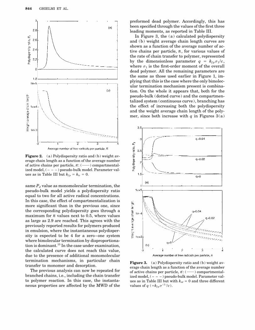
by increasing the entry parameter, r. As expected,the polydispersity values predicted by the com-partmentalized (solid curve) and the pseudo-bulk(dotted curve) models coincide for nV Å 0 as wellas for sufficiently high values of nV . It is worthnoting that in the region where nV ! 1 monomolec-ular terminations are prevailing (since here allbimolecular events are strongly depressed) whilein the region of large nV values bimolecular termi-nations are dominant. Accordingly, in Figure 1the pseudo-bulk model predicts Pd Å 2 and 1.5for low and large nV values, respectively, whichcorrespond to the well known ideal polydispersityvalues for monomolecular and bimolecular bycombination terminations. The effect of compart-mentalization on this behavior can now be ob-served. It can be seen that the solid curve is actu-ally identical in shape to the dotted one, but sim-ply shifted towards larger nV values by an amountequal to about 0.5. This can be explained by con-sidering that, as soon as nV increases above zero, inthe pseudo-bulk system bimolecular terminationsstart to play a role and Pd immediately decreasesbelow two. In the compartmentalized system thiseffect is delayed since there must be a significantamount of particles containing at least two radi-cals before bimolecular termination starts to playa role. Therefore, in this case nV has to increase upto about 0.5 before Pd starts decreasing below 2.A further comment is worth in the case where a Figure 1. (a) Polydispersity ratio and (b) weight av-radical entering the particle terminates immedi- erage chain length as a function of the average numberately with a radical already present in the parti- of active chains per particle, n

V: ( ) compartmental-

cle. In fact, this happens also when nV ! 1. Al- ized model, ( – – – ) pseudo-bulk model. Parameter val-ues as in Table III but kf p Å ktd Å 0.though this is formally a combination reaction, it


844 GHIELMI ET AL.

preformed dead polymer. Accordingly, this hasbeen specified through the values of the first threeleading moments, as reported in Table III.

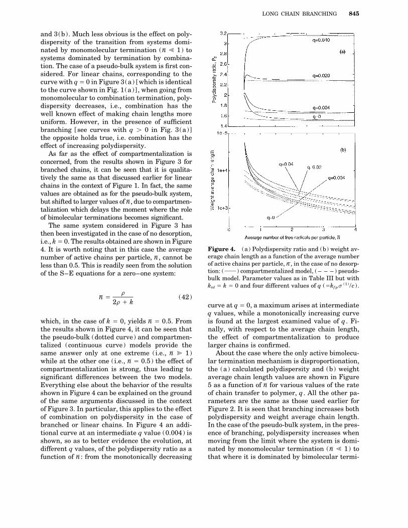
In Figure 3, the (a) calculated polydispersityand (b) weight average chain length curves areshown as a function of the average number of ac-tive chains per particle, nV , for various values ofthe rate of chain transfer to polymer, representedby the dimensionless parameter q Å kf ps1 /c ,where s1 is the first-order moment of the overalldead polymer. All the remaining parameters arethe same as those used earlier in Figure 1, im-plying that this is the case where the only bimolec-ular termination mechanism present is combina-tion. On the whole it appears that, both for thepseudo-bulk (dotted curve) and the compartmen-talized system (continuous curve), branching hasthe effect of increasing both the polydispersityand the weight average chain length of the poly-mer, since both increase with q in Figures 3(a)

Figure 2. (a) Polydispersity ratio and (b) weight av-erage chain length as a function of the average numberof active chains per particle, nV : ( ) compartmental-ized model, ( – – – ) pseudo-bulk model. Parameter val-ues as in Table III but kf p Å ktc Å 0.

same Pd value as monomolecular termination, thepseudo-bulk model yields a polydispersity ratioequal to two for all active radical concentrations.In this case, the effect of compartmentalization ismore significant than in the previous one, sincethe corresponding polydispersity goes through amaximum for nV values next to 0.5, where valuesas large as 2.9 are reached. This agrees with thepreviously reported results for polymers producedin emulsion, where the instantaneous polydisper-sity is expected to be 4 for a zero–one systemwhere bimolecular termination by disproportiona-tion is dominant.15 In the case under examination,the calculated curve does not reach this value,due to the presence of additional monomoleculartermination mechanisms, in particular chain Figure 3. (a) Polydispersity ratio and (b) weight av-transfer to monomer and desorption. erage chain length as a function of the average number

The previous analysis can now be repeated for of active chains per particle, nV : ( ) compartmental-branched chains, i.e., including the chain transfer ized model, ( – – – ) pseudo-bulk model. Parameter val-to polymer reaction. In this case, the instanta- ues as in Table III but with ktd Å 0 and three different

values of q (Åkf ps(1) /c ) .neous properties are affected by the MWD of the



and 3(b). Much less obvious is the effect on poly-dispersity of the transition from systems domi-nated by monomolecular termination (nV ! 1) tosystems dominated by termination by combina-tion. The case of a pseudo-bulk system is first con-sidered. For linear chains, corresponding to thecurve with qÅ 0 in Figure 3(a) [which is identicalto the curve shown in Fig. 1(a)] , when going frommonomolecular to combination termination, poly-dispersity decreases, i.e., combination has thewell known effect of making chain lengths moreuniform. However, in the presence of sufficientbranching [see curves with q ú 0 in Fig. 3(a)]the opposite holds true, i.e. combination has theeffect of increasing polydispersity.

As far as the effect of compartmentalization isconcerned, from the results shown in Figure 3 forbranched chains, it can be seen that it is qualita-tively the same as that discussed earlier for linearchains in the context of Figure 1. In fact, the samevalues are obtained as for the pseudo-bulk system,but shifted to larger values of nV , due to compartmen-talization which delays the moment where the roleof bimolecular terminations becomes significant.

The same system considered in Figure 3 hasthen been investigated in the case of no desorption,i.e., kÅ 0. The results obtained are shown in Figure

Figure 4. (a) Polydispersity ratio and (b) weight av-4. It is worth noting that in this case the averageerage chain length as a function of the average numbernumber of active chains per particle, nV , cannot beof active chains per particle, n

V, in the case of no desorp-less than 0.5. This is readily seen from the solution

tion: ( ) compartmentalized model, ( – – – ) pseudo-of the S–E equations for a zero–one system:bulk model. Parameter values as in Table III but withktd Å k Å 0 and four different values of q (Åkf ps

(1) /c ) .

nV År

2r / k(42)

curve at q Å 0, a maximum arises at intermediateq values, while a monotonically increasing curveis found at the largest examined value of q . Fi-which, in the case of k Å 0, yields nV Å 0.5. From

the results shown in Figure 4, it can be seen that nally, with respect to the average chain length,the effect of compartmentalization to producethe pseudo-bulk (dotted curve) and compartmen-

talized (continuous curve) models provide the larger chains is confirmed.About the case where the only active bimolecu-same answer only at one extreme (i.e., nV @ 1)

while at the other one (i.e., nV Å 0.5) the effect of lar termination mechanism is disproportionation,the (a) calculated polydispersity and (b) weightcompartmentalization is strong, thus leading to

significant differences between the two models. average chain length values are shown in Figure5 as a function of nV for various values of the rateEverything else about the behavior of the results

shown in Figure 4 can be explained on the ground of chain transfer to polymer, q . All the other pa-rameters are the same as those used earlier forof the same arguments discussed in the context

of Figure 3. In particular, this applies to the effect Figure 2. It is seen that branching increases bothpolydispersity and weight average chain length.of combination on polydispersity in the case of

branched or linear chains. In Figure 4 an addi- In the case of the pseudo-bulk system, in the pres-ence of branching, polydispersity increases whentional curve at an intermediate q value (0.004) is

shown, so as to better evidence the evolution, at moving from the limit where the system is domi-nated by monomolecular termination (nV ! 1) todifferent q values, of the polydispersity ratio as a

function of nV : from the monotonically decreasing that where it is dominated by bimolecular termi-


846 GHIELMI ET AL.

tive rather than instantaneous properties. This isso because the chemical mechanism which pro-duces branched polymer chains acts on the pre-formed dead polymer, which is characterized bythe cumulative quantities.

To calculate the cumulative properties of thepolymer, the kinetic model developed in this workhas to be linked to another model which simulatesthe emulsion polymerization process at a macro-scale. In particular, a model discussed by Stortiet al.25 has been used, which evaluates the timeevolution of the typical quantities of an emulsionpolymerization: concentrations of monomer, poly-mer, emulsifier and initiator. Moreover, thismodel accounts for diffusive limitations on therate constants as a function of conversion and pro-vides kinetic expressions for radical entry intoand exit from the polymer particles.

The adopted numerical values of the model pa-rameters are reported in Table IV. They corre-spond to a typical emulsion polymerization pro-cess where a chain transfer to polymer reactionis present, leading to polymer gelation at a conver-sion value slightly larger than 90%. Moreover, aseeded polymerization has been considered, thussimulating intervals II and III of the emulsionpolymerization process only, so as to avoid the

Figure 5. (a) Polydispersity ratio and (b) weight av- simulation of the particle nucleation stage. Thiserage chain length as a function of the average number implies that particle volume monodispersion canof active chains per particle, n

V: ( ) compartmental- be assumed. The seed causes the reaction to start

ized model, ( – – – ) pseudo-bulk model. Parameter val- from about 15% conversion and its influence onues as in Table III but with ktc Å 0 and three different the cumulative properties decreases as the reac-values of q (Åkf ps

(1) /c ) . tion proceeds. Table IV reports also the character-istics of the seed.

nation by disproportionation. The effect of com- The conversion profile obtained as a functionpartmentalization, besides shifting the value of n

V of time (not reported) exhibits the expected be-at which bimolecular termination overtakes the havior, whereas more interesting remarks can bemonomolecular ones, is to produce a maximum made on the time evolution of the average numberin polydispersity at about n

VÅ 0.5, typical of the of active chains per particle. Increasing values of

termination by disproportionation mechanism. nV are observed, namely from nV Å 0.5 (initial zero–From the results above it can be concluded that one system) up to about 1.5. This is due to the

the role of chain compartmentalization on the Trommsdorff effect which causes the terminationMWD of a polymer produced in emulsion is im- by combination frequency constant, c , to decrease.portant for both linear and branched chains. The increasing value of nV produces increasingUsing a pseudo-bulk model for calculating the mo- values of the ratio between termination by com-lecular weight distribution in an emulsion poly- bination and monomolecular termination rates,merization system can introduce significant inac- namely chain transfer to monomer. This is furthercuracies, particularly in the range of values 0õ n

V enhanced by the progressive decrease of theõ 2 (typical of these systems), even when dealing monomer to polymer ratio in the particle, with awith instantaneous properties. corresponding increase of the rate of chain trans-

fer to polymer. All these effects, and in particularCUMULATIVE PROPERTIES the growth of the kinetic mechanism responsiblefor gelation (i.e., termination by combination inIt is probably more significant to analyze the role

of chain transfer to polymer in terms of cumula- the presence of branched chains), allow us to ex-



Table IV. Numerical Values of the Model Parameters Usedfor the Illustrative Calculations of Cumulative Properties

Symbol Value Meaning

aM 5.54 1 108 cm2/mol Molecular surface of the micellar emulsifierB 0.939 Trommsdorff effect parameter25

C 3.875 Trommsdorff effect parameter25

C`e,a 4.74 1 10010 mol/cm2 Surface adsorbed emulsifier concentration at saturation

CMC 1.77 1 1006 mol/cm3H2O Critical micellar concentration

Csatm,w 3.68 1 1006 mol/cm3

H2O Monomer water concentration at saturationD 00.494 Trommsdorff effect parameter25

ke 2 1 10013 cm3/s Entry rate constantkfm 9.07 cm3/(mol s) Chain transfer to monomer rate constantkfp 30 cm3/(mol s) Chain transfer to polymer rate constantki 1.18 1 1006 1/s Initiator decomposition rate constantkp 2.59 1 105 cm3/(mol s) Propagation rate constantktc 5.97 1 109 cm3/(mol s) Termination by combination rate constantktd 0 cm3/(mol s) Termination by disproportionation rate constantM seed

n 1 1 104 Seed number average chain lengthNP 1 1 1014 1/cm3

H2O Particles concentrationP seed

d 2 Seed polydispersity ratioPMe 288.5 g/mol Emulsifier molecular weightPMi 270.31 g/mol Initiator molecular weightPMm 104.2 g/mol Monomer molecular weightQe 3.8 g Feed emulsifierQi 0.584 g Feed initiatorVm 113.8 cm3 Feed monomer volumeVP,0 5 1 10016 cm3 Initial particle volumeVw 1012.3 cm3 Feed waterh 1.0 Initiator efficiencyf* 0.68 Particle monomer volume fraction at saturationrm 0.878 g/cm3 Monomer densityrp 1.05 g/cm3 Polymer density

pect that gel formation will occur at a certain con- with those corresponding to the case of linearchains (i.e., q Å 0). Before the gel point, the num-version value and, in fact, this is predicted by the

model. In Figure 6 the gel weight fraction is re- ber average chain length is not influenced bychain transfer to polymer, while the weight aver-ported as a function of time for various values of

NG , i.e. the number of generations adopted in age chain length increases as the reaction pro-ceeds, due to the continuous formation ofthe numerical fractionation technique described

above. The results of the calculations performed branched chains. As soon as the gel point isreached the curves in the figure show a sharpat an increasing number of generations (from 3

to 8) show a convergence in the predicted outset discontinuity of the derivative: this is an effect ofthe gel polymer growth, which causes a continu-of gel formation at about 190 min. The results

obtained allow us to select NG Å 7 as the mini- ous extraction of the polymer from the sol fraction.After this critical time, the polymer chains belong-mum number of generations to be used in the frac-

tionation procedure to obtain reliable predictions. ing to the highest generations are the first to dis-appear, and the polydispersity ratio of the solThese results do not deserve further comments,

since they are qualitatively similar to those ob- polymer decreases.The observed behavior of the overall propertiestained by Teymour and Campbell17 for a bulk sys-

tem and are characteristic of the numerical frac- close to the gel point may be better understood byexamining the evolution of the first order momenttionation technique adopted.

In Figure 7 the evolution of the number and for each generation of the sol polymer, shown inFigure 8. The different curves are identified byweight average chain lengths of the sol polymer

are shown as a function of time and compared the generation index, g ; note that g Å 0 indicates


848 GHIELMI ET AL.

Figure 6. Gel weight fraction as a function of time at Figure 8. First order moments for each generationan increasing number of branched generations, NG . as a function of time (g Å 0 indicates linear chains).Parameter values as in Table IV. Parameter values as in Table IV.

linear chains. The effect of sol polymer extraction be observed as the result of the superimpositionby the gelified polymer is once more evident and of several homogeneous classes. The distributionits role can be seen to increase with the generation of each generation has been reconstructed usingindex. As a limit behavior, the highest genera-tions are formed and disappear around the gelpoint and this is the reason for the numerical con-vergence shown in Figure 6: highest order genera-tions are quickly vanishing and of negligibleamount. The maxima in the first moment vs. con-version or time curves of the highest generationsidentify the gel point.

The overall weight distribution of the polymer-ization degree of the sol fraction has been calcu-lated before and after the gel point. The distribu-tion is shown in Figure 9 together with the contri-butions of each sol generation, scaled by theirrespective first moments. A complex behavior can

Figure 9. Overall weight distribution of the polymer-ization degree (a) before and (b) after the gel point onhorizontal logarithmic scale. Parameter values as inFigure 7. Number and weight average chain length

as a function of time. Parameter values as in Table IV. Table IV.



the Schultz distribution26 as model distribution,thus using the first three moments only. The accu-racy of this procedure could be questionable whenthe distribution under examination is too differ-ent from the selected model distribution, i.e.,when it is too wide and complex.27 Thus, as a testof the reliability of the calculated distributions,the polydispersity ratios for each generation areshown in Figure 10 as a function of time. Noticethat, apart from linear and first branched genera-tions, these values are surprisingly low and, inparticular, less than 2. This is an indirect checkof the effectiveness of the adopted fractionationtechnique. However, the first two classes (g Å 0and g Å 1) exhibit increasing polydispersity ra- Figure 11. Tail ends of the polymerization degree dis-tios, to the extent that they may affect the reliabil- tribution at increasing conversions. Parameter valuesity of the reconstructed distributions shown in as in Table IV.Figure 9 and, in particular, their bimodal nature.To overcome this difficulty, the fractionation rules

Effect of Termination by Combinationcould be improved so as to increase the ‘‘selectiv-ity’’ with respect to the polymer chains of the first To investigate the effect of bimolecular termina-

tion by combination on the properties of thetwo generations. In this direction, some effort hasbeen made and reported very recently in the liter- formed polymer and on the gel point, a compari-

son has been made between two simulations withature.28 Here this problem will not be further ex-amined. different values of the combination rate constant.

The first simulation has been performed using theFinally in Figure 11 the tail ends of the poly-merization degree distribution are shown at four parameter values of Table IV, while in the other

one ktc has been increased by one order of magni-different times, two before and two after the gelpoint. Notice that approaching the gel point the tude, with the other parameters unchanged.

A different behavior of nV values can be observedtail ends move to high chain length values (curvesat 82 and 92% conversion), while after the gel in the two cases. In Figure 12(a) the average

number of active chains per particle is plotted aspoint they move back to lower values. This behav-ior confirms the effect of the extraction of macro- a function of conversion. As expected, in the case

of larger ktc , the curve for nV lies below the othermolecules with large polymerization degrees dueto gel formation. one, slightly exceeding 0.6, while it reaches 1.5

for the lower value of ktc .By analyzing the rates of the various termina-

tion mechanisms, it can be seen that these aresubstantially unchanged in the two cases. A com-pensation between the increased value of ktc andthe subsequently decreased number of particlescontaining at least two radicals can be observed,which leads to comparable rates of the bimolecu-lar termination by combination reaction. Thismechanism is less important than monomoleculartermination mechanisms at low conversion val-ues, while it becomes prevalent above about 65%conversion, thus leading to gelation. Gelation oc-curs earlier in the case of a lower ktc value, sincelarger nV imply a larger rate of the branching reac-tion. Thus, it can be concluded that, at least in thiscase, lower ktc values favor gelation. This result isFigure 10. Polydispersity ratios for each generationapparently in contrast with the mechanism of gelas a function of time (g Å 0 indicates linear chains).

Parameter values as in Table IV. formation discussed earlier. According to this,


850 GHIELMI ET AL.

tial amount of polymer to be the same in the twocases, but with different values of the initial parti-cle volume VP0 . The first simulation has been per-formed using the values of the parameters in Ta-ble IV, while for the second the initial particlevolume has been assumed to be doubled and theinitial number of particles per unit volume of wa-ter halved, with the other parameters unchanged.

In Figure 13(a) the average number of activechains per particle nV is shown as a function ofconversion for the two different initial volumes.At larger VP values the bimolecular terminationfrequency c Å ktc /2NAVP is lower and, therefore,the corresponding nV values are larger.

By analyzing the rates of the various involvedtermination mechanisms, it is found that, in thecase of larger VP values, the accumulation of radi-cals in the particles due to the decreased bimolec-ular termination constant c , leads to an increaseof the number of dead polymer chains produced

Figure 12. (a) Average number of free radicals perparticle and (b) number and weight average chainlength as a function of conversion, for two different val-ues of the bimolecular termination rate constant, ktc .Other parameter values as in Table IV.

since gelation occurs because of the combinationbetween branched chains, one would expect largervalues of the termination by combination constantto lead to earlier gelation, which is not the casein the instance shown in Figure 12(b). This isdue to radical compartmentalization in emulsionpolymerization systems, which prevents a sig-nificant increase of the dead polymer chains pro-duced by bimolecular termination (even thoughktc is increased). Instead, the accumulation of ac-tive chains in the polymer particles obtained atsmaller values of ktc increases the degree ofbranching and therefore makes gelation morelikely to occur.

Figure 13. (a) Average number of free radicals perparticle and (b) number and weight average chainEffect of the Particle Volumelength as a function of conversion, for two different val-

The role of the particle volume has been investi- ues of the seed initial particle volume, VP0 . Other pa-gated by simulating two seeded polymerizations. rameter values as in Table IV, except for the particle

concentration NP .The seeds have been selected by requiring the ini-



by bimolecular combination. Since also the strate the applicability of the model to the predic-tion of both the pre- and post-gelation phases ofbranching reaction is favored by larger nV values,

it results that gelation is favored. This can be seen the process. In particular, the MWD of the solpolymer fraction can be determined during allin Figure 13(b), where the number and weight

average chain lengths are shown as a function of phases of polymerization.Finally, evidence for some unexpected behaviorconversion, indicating that gelation occurs first

for larger particle volumes of the seed. If the of the polymer MWD and of the occurrence of gela-tion has been obtained through a series of simula-mechanism of gel formation discussed earlier is

recalled, which requires that bimolecular termi- tions involving some parameters peculiar to emul-sion polymerizations (i.e., the bimolecular termi-nation by combination be responsible for gelation,

the fact that gel is formed earlier at lower values nation by combination rate constant and theparticle volume). These results show clearly theof the pseudo-first-order termination rate con-

stant c , is again an unexpected result. Once more, need for detailed models to predict the molecularweight properties of the product and the gel for-this apparent contradiction is a clear effect of rad-

ical compartmentalization in emulsion polymer- mation in emulsion polymerizations. This is be-cause the interactions between the phenomenaization systems.typical of this kind of reactions, such as compart-mentalization, radical accumulation in the poly-mer particles, chain branching and bimolecularCONCLUSIONStermination, may be rather complex.

In this work, a model has been developed for eval-uating the MWD of a polymer produced in an APPENDIX I: FRACTIONATED EQUATIONSemulsion process when a kinetic mechanism forlong chain branching is active, namely chain When the numerical fractionation technique istransfer to polymer. This model combines a ki- applied, all quantities referring to polymernetic model, developed to describe linear polymer chains, both active and dead, must be labelled bychains in emulsion polymerization, and a recently an index specifying which generation the chainproposed technique, i.e. numerical fractionation, belongs to. Doubly distinguished particle distribu-introduced to calculate the MWD of branched tions require two generation indices, since therepolymer chains formed in bulk polymerizations are two distinguishing chains. This holds also forbefore and after the gel point. These two ap- the distribution of the dead polymer produced byproaches, together with the new concept of chain the bimolecular termination of pairs of chains,pre-life, allow the calculation of the MWD of since the generation of the resulting chain is de-branched polymer chains produced in emulsion, termined by the generations which the two termi-as well as the description of the formation of a gel nating chains belong to.phase. Using this model, a rigorous analysis of The polymer population is subdivided into gen-the role of chain compartmentalization, both in erations by labelling linear chains by the index 0terms of instantaneous and cumulative proper- and branched chains by an index g , with g Å 1,ties, has been developed. The former have been . . . , NG , being NG the maximum number ofstudied in parallel with the results obtained fol- branched generations adopted. Accordingly, therelowing the approximate approach which consists is no longer a need for the singly distinguishedin forcing a bulk model to describe an emulsion particle distributions to be represented by two dif-system (the so called pseudo-bulk model) . The ferent symbols N *i and B *i , since the generationcomparison allows the role of compartmentaliza- index immediately evidences if the distinguishingtion in determining the peculiarities of emulsion chain is linear or branched. Thus, a single symbolproduced polymers to be well characterized. The B *i ,g = is adopted. When g * Å 0 the chain is linearsimplified approach to molecular weight calcula- and the distribution does not depend on pre-lifetions based on a pseudo-bulk model has been n *. In all other cases, i.e., for g * ¢ 1, B*g =

Å B*i ,g =(t , t *, n * ) . Similarly, doubly distinguishedproved inadequate.With reference to cumulative properties, the particle distributions can be represented by a sin-

gle symbol labelled by two generation indices:model developed has been combined with a kineticmodel of emulsion polymerization in order to cal- B 9i ,g =,g 0 . If g * Å 0 the older distinguishing chain is

linear, i.e., n * Å 0; if g 9 Å 0 the younger chain isculate the MWD of the polymer formed during thereaction. The simulation results obtained demon- linear, i.e., n 9 Å 0.


852 GHIELMI ET AL.

The equations resulting from the application of active chain of the first branched generation. Inall other cases, chain transfer to polymer yieldsnumerical fractionation are similar to the original

equations reported earlier. Differences arise only an active chain of the same generation of the in-volved dead chain.when transitions of polymer chains from one gen-

eration to another must be accounted for.

Doubly Distinguished ParticlesSingly Distinguished Particles

Similarly to the previous case, the equations de-scribing the evolution of the doubly distinguishedThe differential system describing the evolution

of the singly distinguished particle distributions, particle distributions are independent of the gen-eration indices g * and g 9 are identical to eqs. (6).B *i ,g = , does not depend on the value of the indexBy introducing the column vector B 9g =,g 0 they cang * and coincides with that written for the overallbe written in matrix form as:distribution given by eq. (3). It can be written

synthetically in matrix form as:ÌB 9g =,g 0

Ìt 9Å D (t )B 9g =,g 0 (A5)ÌB *g =

Ìt *Å A (t )B *g = , (A1)

where D is the same band matrix used in eq. (33).The form of the initial conditions depends onwhere A is the same band matrix used in eq. (24).

the value of the generation index g 9:Note that the moment s (1) appearing in the diago-nal terms of this matrix accounts for the overall

• g 9 Å 0dead polymer, i.e., both sol and gel fractions ifgelation occurred, since an active chain can give

B 9i ,g =,0 (t , t *, t 9 Å 0, n * )chain transfer to any dead chain.Although the equations describing the singly

Å rB *i01,g =(t , t *, n * )distinguished particle distributions do not dependon the generation index g *, the initial conditions / kf mCm( i 0 1)B *i ,g =(t , t *, n * ) (A6)do, according to the following scheme:

• g 9 Å 1• g * Å 0

B 9i ,g =,1 (t , t *, t 9 Å 0, n *, n 9 )B *i ,0 (t , t * Å 0)

Å kf p ( i 0 1)B *i ,g =(t , t *, n * )n 9Å rNi01(t ) / kf mCmiNi (t ) (A2)1 [D0(t , n 9 ) / D1(t , n 9 ) ] (A7)

• g * Å 1• g 9 ¢ 2

B *i ,1 (t , t * Å 0, n * ) Å kf piNi (t )n *B 9i ,g =,g 0 (t , t *, t 9 Å 0, n *, n 9 )1 [D1(t , n * ) / D0(t , n * ) ] (A3)

• g * ¢ 2 Å kf p ( i 0 1)B *i ,g =(t , t *, n * )

1 n 9Dg 0(t , n 9 ) (A8)B *i ,g = (t , t * Å 0, n * )

Å kf piNi (t )n*Dg =(t , n * ) (A4)where 2 ° i ° N and 0 ° g * ° NG (with n * Å 0when g * Å 0).

where 1 ° i ° N and Dg =(t , n * ) is the CLD of thedead polymer of generation g *. These equations Polymer Formed by Monomolecular Terminationhave been derived considering that an active lin-ear chain can be generated only through radical As for the active chain distributions, a single sym-

bol can be used to describe the distributions GMg *entry or transfer to monomer, while chain trans-

fer to polymer causes generation transfer only of the polymer belonging to a certain generationwhich has been formed by monomolecular termi-when it affects a linear dead chain, producing an



nation. This follows again from the presence of Polymer Formed by Combinationthe generation index g *, which indicates whether

Two generation indices are used to label the dis-the chain is linear or branched.tributions GC

g =,g 0 of the polymer chains terminatedThe equations describing the distributionsby combination, corresponding to the generationGM

g = do not depend on the generation index g * andindices of the two active chains from which thehave the same structure as the equations for thedead chain derived. Note that at this point thecorresponding overall distribution derived earlier.generation of the resulting dead chain is not to beThis is because no monomolecular terminationcomputed and, therefore, no terms in the equa-event causes an active chain to undergo a genera-tions must account for generation transitions.tion transfer on dying. Thus, for 0 ° g * ° NG :Thus, once more the resulting equation is identi-cal to that written earlier for the overall distribu-tion of the polymer terminated by combination:d[VPGM

g = (te , t *, n * ) ]dte

Å [ (k / kf mCm / kf ps(1) ) d[VPGC

g =,g 0(te , t *, t 9, n *, n 9 ) ]dte

1 ∑N

iÅ1

B *i ,g =(te 0 t *, t *, n * )Å [2cc ∑

N

iÅ2

B 9i ,g =,g 0(te 0 t * 0 t 9, t *, t 9, n *, n 9 )

/ r

NB *N ,g =(te 0 t *, t *, n * )

0 kf pnGCg =,g 0(te , t *, t 9, n *, n 9 ) ∑

N

iÅ1

iNi ]1

NA/ 2cd ∑N

iÅ2

( i 0 1)B *i ,g =(te 0 t *, t *, n * )(A10)

0 kf pnGMg = (te , t *, n * ) ∑

N

iÅ1

iNi ]1

NA, (A9) where n is the length of the dead chain, which

depends on the generation indices as reported inTable AI.where n is the length of the dead chain, given by

Equation (A10) holds for 0 ° g *, g 9 ° NG .n Å n * / at * in the case where g * ¢ 1. When g *However, when g *Å 0 or g 9Å 0, there is no depen-Å 0, the pre-life of the active chain producing thedence on n * or n 9 respectively.dead polymer chain is zero. Accordingly, the de-

pendence on n * must be eliminated in eq. (A9)[GM

0 Å GM0 (te , t * ) ] and the chain length is n Å at *. Moment Equations

The chain length n of the dead polymer chain issummarized in Table AI according to the genera- The moments of all the fractionated distributions

introduced above are defined in analogy with thetion index.

Table AI. Fractionated Dead Chain Distributions and Corresponding Chain Lengths

Distribution of thePolymer Terminated Generation of the

Monomolecularly Chain Chain Length

GM0 (te , t * ) 0 at *

GMg= (te , t *, n * ) g * ¢ 1 n * / at *

Distribution of thePolymer Terminated by Generation of the Generation of the

Combination Older Chain Younger Chain Chain Length

GC0,0 (te , t *, t 9 ) 0 0 a(t * / 2t 9 )

GCg=,0 (te , t *, t 9, n * ) g * ¢ 1 0 n * / a(t * / 2t 9 )

GC0,g0 (te , t *, t 9, n 9 ) 0 g 9 ¢ 1 n 9 / a(t * / 2t 9 )

GCg=,g0 (te , t *, t 9, n *, n 9 ) g * ¢ 1 g 9 ¢ 1 n * / n 9 / a(t * / 2t 9 )


854 GHIELMI ET AL.

overall moments defined earlier. Likewise, their bination between two chains of different genera-tions gives a chain belonging to the higher one.evaluation is rather similar.

The moments of the singly and doubly distin- The combination between two chains of the samegeneration g¢ 1 gives a chain belonging to gener-guished particle distributions can be obtained by

applying the moment definition to eqs. (A1) and ation g / 1. Accordingly, the relationships which(A5) and then integrating by parts. The resulting allow to obtain s (k )

C ,g from sV

(k )C ,g =,g 0 are given by:

equations, reported in Tables AII and AIII, implythe solution of sets of algebraic systems. The inte- • g Å 0grated initial conditions appearing on the right-hand side can be evaluated using eqs. (A2) – (A4) s (k )

C ,0 Å sV

(k )C ,0,0 (A13)

and (A6) – (A8).The moment equations of the polymer formed • g Å 1

by monomolecular termination and by combina-tion, s (k )

M ,g = and sV

(k )C ,g =,g 0 respectively, can be obtained s (k )

C ,1 Å sV

(k )C ,1,0 / s

V

(k )C ,0,1 (A14)

from eqs. (A9) and (A10) by applying the momentdefinition to both sides. It must be observed that • g ¢ 2moment s

V

(k )C ,g =,g 0 , similarly to distribution GC

g =,g 0

from which it takes origin, accounts for both gen-s(k)

C,gÅ ∑g01

rÅ0

(sV

(k)C,r,g / s

V

(k)C,g,r) / s

V

(k)C,g01,g01 (A15)

erations of the active chains which produced thedead chain, disregarding the generation of the re-sulting chain. The moment equations are the fol- The overall moments of the dead polymer oflowing: generation g can be evaluated by summing up the

moments of the polymer formed by monomolecu-• Polymer formed by monomolecular termina- lar termination and by combination:

tions (k )

g Å s (k )M ,g / s (k )

C ,g (A16)d[VPs

(k )M ,g =]

dteThe resulting overall moment equations for

each generation follow from the application of re-lationships (A13) – (A16) to eqs. (A11) andÅ [ (k/ kf mCm/ kf ps

(1) ) ∑N

iÅ1

r * (k )i ,g = /

r

Nr * (k )

N ,g = (A12), as reported in Table AIV. Note that these

/ 2cd ∑N

iÅ2

( i0 1)r * (k )i ,g =

Table AII. Fractionated Moment Equations of theSingly Distinguished Particle Distributions

0 kf ps(k/1)M ,g = ∑

N

iÅ1

iNi ]1

NA(A11)

g * Å 0

rk Å 0 A r *(0)0 Å 0B *0(t, t * Å 0)

• polymer formed by combination

rk ¢ 1 A r *(k )0 Å 0akr *(k01)

0d[VPsV(k )C ,g =,g 0]

dteÅ [2cc ∑

N

iÅ2

r 9 (k )i ,g =,g 0

g * ¢ 1

0 kf psV(k )C ,g =,g 0 ∑

N

iÅ1

iNi ]1

NA(A12) A r *(k)

g= Å 0*`

0(n * )kB *g= (t , t * Å 0, n * ) dn * 0 akr *(k01)

g=

where (i Å 1, . . . , N ):

Finally, the moment s (k )C ,g of the polymer of gen-

rg * Å 1 *`

0(n * )kB *i,1 (t, t * Å 0, n * ) dn *eration g terminated by combination can be ob-Å kfpiNi [s (k/1)

0 / s (k/1)1 ]tained from the quantities s

V

(k )C ,g =,g 0 by properly

applying the transfer rules between generations.rg * ¢ 2 *

`

0(n * )kB *i,g= (t, t * Å 0, n * ) dn *It is sufficient to recall that the combination be-

tween two linear active chains yields a linear dead Å kfpiNis(k/1)g=chain, thus belonging to generation zero. The com-



Table AIII. Fractionated Moment Equations of the Doubly Distinguished ParticleDistributions

g * Å 0, g 9 Å 0

D r 9(k )0,0 Å 02akr 9(k01)

0,0 0 *`

0(at * )kB 90,0 (t, t *, t 9 Å 0) dt *

where (i Å 2, . . . , N ):

*`

0(at * )kB 9i,0,0 (t, t *, t 9 Å 0) dt * Å rr*(k )

i01,0 / kfmCm (i 0 1)r*(k)i,0

g * ¢ 1, g 9 Å 0

D r 9(k)=,0 Å 02akr9(k01)

g=,0 0 *`

0*

`

0(n * / at * )kB 9g=,0 (t, t *, t 9 Å 0, n * ) dt * dn *

where (i Å 2, . . . , N ):

*`

0*

`

0(n * / at * )kB 9i,g=,0(t, t *, t 9 Å 0, n * ) dt * dn * Å rr*(k)

i01,g= / kfmCm (i 0 1)r *(k)i,g=

g * Å 0, g 9 ¢ 1

D r 9(k )0,g0 Å 02akr 9(k01)

0,g0 0 *`

0*

`

0(n 9 / at * )kB 90,g0 (t, t *, t 9 Å 0, n 9 ) dt * dn 9

where (i Å 2, . . . , N ):

rg 9 Å 1 *`

0*

`

0(n 9 / at * )kB 9i,0,1 (t, t *, t 9 Å 0, n 9) dt * dn 9

Å kfp (i 0 1) (k

jÅ0Sk

jD r *(k0j )i,0 [s( j/1)

0 / s ( j/1)1 ]

rg 9 ¢ 2 *`

0*

`

0(n 9 / at * )kB 9i,0,g0 (t, t *, t 9 Å 0, n 9) dt * dn 9

Å kfp (i 0 1) (k

jÅ0Sk

jD r *(k0j )i,0 s( j/1)

g0

g * ¢ 1, g 9 ¢ 1

D r 9(k)g=,g0 Å 02akr 9(k01)

g=,g0 0 *`

0*

`

0*

`

0(n * / n 9 / at * )kB 9g=,g0 (t, t *, t 9 Å 0, n *, n 9 ) dt * dn * dn 9

where (i Å 2, . . . , N ):

rg 9 Å 1 *`

0*

`

0*

`

0(n * / n 9 / at * )kB 9i,g=,1 (t, t *, t 9 Å 0, n *, n 9) dt * dn * dn 9

Å kfp (i 0 1) (k

jÅ0Sk

jD r *(k0j )i,g= [s( j/1)

0 / s ( j/1)1 ]

rg 9 ¢ 2 *`

0*

`

0*

`

0(n * / n 9 / at * )kB 9i,g=,g0(t, t *, t 9 Å 0, n *, n 9) dt * dn * dn 9

Å kfp (i 0 1) (k

jÅ0Sk

jD r *(k0j )i,g= s( j/1)

g0


856 GHIELMI ET AL.

Table AIV. Fractionated Moment Equations of the Dead Polymer

g Å 0

d[VPs(k )0 ]


(1)) (N

iÅ1r *(k )

i,0 / r

Nr *(k )

N,0 / 2cd (N

iÅ2(i 0 1)r *(k )

i,0

/ 2cc (N

iÅ2r 9(k)

i,0,0 0 kfps(k/1)0 (

N

iÅ1iNi ]

1NA

g Å 1

d[VPs(k )1 ]


(1)) (N

iÅ1r *(k )

i,1 / r

Nr *(k )

N,1

/ 2cd (N

iÅ2(i 0 1)r *(k )

i,1 / 2cc (N

iÅ2(r 9(k)

i,1,0 / r 9(k)i,0,1 ) 0 kfps

(k/1)1 (

N

iÅ1iNi ]

1NA

g ¢ 2

d[VPs(k )g ]


(1)) (N

iÅ1r *(k )

i,g / r

Nr *(k )

N,g / 2cd (N

iÅ2(i 0 1)r *(k )

i,g

/ 2cc (N

iÅ2( (g01

rÅ0(r 9(k)

i,r,g / r 9(k)i,g,r) / r 9(k )

i,g01,g01) 0 kfps(k/1)g (

N

iÅ1iNi ]

1NA

Closure equation:

s (3)g Å 2

(s (2)g )2

s (1)g

0 s (2)g s (1)

g

s (0)g

equations provide evidence for the occurrence of For this purpose, definition (A17) can be ap-plied to eq. (11), thus obtaining:a closure problem, since every moment depends

on the next higher. However, since each genera-tion is expected to be homogeneous enough, the

s (k )M Å *

`

0nkDM (te , n ) dnsimple closure equation reported in Table AIV has

been used. This equation results from the modelÅ *

`

0nk dn *

n /a

0GM (te , t *, n 0 at * ) dt *distribution selected for the reconstruction of the

CLDs and is reliable if three moments only aresufficient for an accurate description of the CLD

/ *`

0nk 1

aSMSte ,

naD dnof each generation.9

Tables AII–AIV summarize the equationsneeded for the computation of the moments of

Å *`

0dt * *

`

at =nkGM (te , t *, n 0 at * ) dnthe MWD.

/ *`

0nk 1

aSMSte ,

naD dnAPPENDIX II

The aim of this appendix is to show that the mo-ments of the distributions GM (te , t *, n * ) and Recalling that for the branched contribution nSM (te , t * ) , defined through eqs. (21) and (22), Å n * / at * and that for the linear one n Å at *,respectively, are equivalent to those of the chain the demonstration can be completed:length distribution DM (te , n ) of the polymerformed by monomolecular termination according

s (k )M Å *

`

0dt * *

`

0(n* / at * )kGM (te , t *, n * ) dn *to the usual definition of moment:

s (k )M Å *

`

0nkDM (te , n ) dn (A17) / *

`

0(at * )kSM (te , t * ) dt * Å s (k )

G ,M / s (k )S ,M



cd termination by disproportionation fre-APPENDIX III: PSEUDO-BULK MODELquency, s01

The equations of the pseudo-bulk model used for Cm monomer concentration in the particles,comparison with the compartmentalized model mol cm03

developed in this work are summarized in the fol- D matrix of the coefficients of the balancelowing: system for doubly distinguished parti-

clesD CLD of the dead polymerr (1) Å (1 / t / b / cps

(2) )(t / b / cps

(1) )r (0)

DC CLD of the polymer terminated by combi-nation

DM CLD of the polymer terminated monomo-ds (0)

dtÅ kpCmr

(0)St / b

2D lecularlyDg CLD of the dead polymer of generation gg * generation of the older distinguishingds (1)

dtÅ kpCmr

(0) (1 / t / b )chain

g 9 generation of the younger distinguishingds (2)

dtÅ kpCmr

(0) chainGC distribution of the polymer terminated by

combination coming from a pair of dis-1 F1 / t / b / 2r (1)

r (0) / bSr (1)

r (0)D2G (A18) tinguishing chains, both branchedGM distribution of the polymer terminated

monomolecularly, branchedwhere s ( j ) and r ( j ) are the jth order moments GC

g =,g 0 fractionated distribution of the polymerof the dead and active polymer, respectively. The terminated by combinationparameter cp Å kf p / (kpCm ) accounts for chain GM

g = fractionated distribution of the polymertransfer to polymer, while t and b account for terminated monomolecularlymonomolecular and bimolecular termination, re- k desorption frequency, s01

spectively. In particular, t takes into account also ke rate constant for entry, cm3 s01

the typical emulsion reaction mechanisms, such kf m rate constant for chain transfer to mono-as desorption and entry: mer, cm3 mol01 s01

kf p rate constant for chain transfer to poly-mer, cm3 mol01 s01

t Å kf mCm / ktdr(0) / k / rNN

kpCm kp rate constant for chain propagation, cm3

mol01 s01

b Å ktcr(0)

kpCmktc rate constant for termination by combina-

tion, cm3 mol01 s01

ktd rate constant for termination by dispro-portionation, cm3 mol01 s01APPENDIX IV: NOMENCLATURE

n number of monomeric units bound to achainA matrix of the coefficients of the balance

system for singly distinguished parti- n * pre-life of the older distinguishing chainn 9 pre-life of the younger distinguishingcles

distribution of the singly distinguished chainB *iparticles, branched nV average number of free radicals per par-

ticledistribution of the doubly distinguishedB 9iparticles, branched N maximum number of free radicals in a

particlefractionated distribution of the singly dis-B *i ,g =tinguished particles NA Avogadro’s number

Ni distribution of the particles containing ifractionated distribution of the doublyB 9i ,g =,g 0

distinguished particles radicalsdistribution of the singly distinguishedc Å (cc / cd ) , overall bimolecular termina- N *i

particles, lineartion frequency, s01

cc termination by combination frequency, distribution of the doubly distinguishedN 9iparticles, linears01


858 GHIELMI ET AL.

NG number of branched generations REFERENCES AND NOTESdistribution of the doubly distinguishedO 9i 1. J. L. Gardon, J. Polym. Sci. A-1, 6, 623 (1968).particles with the older distinguishing

2. S. Katz, R. Shinnar, and G. M. Saidel, Adv. Chem.chain branchedSer., 91, 145 (1969).Pd polydispersity ratio 3. K. W. Min and W. H. Ray, J. Macromol. Sci. Rev.

Pn dead polymer chain of length n Macromol. Chem., C11, 177 (1974).q dimensionless parameter for chain trans- 4. G. Lichti, R. G. Gilbert, and D. H. Napper, J.

fer to polymer Polym. Sci. Polym. Chem. Ed., 18, 1292 (1980).R•

n active polymer chain of length n 5. P. A. Clay and R. G. Gilbert, Macromolecules, 28,552 (1995).R•

w water phase concentration of the active6. G. Storti, G. Polotti, M. Cociani, and M. Morbidelli,radicals

J. Polym. Sci. Part A: Polym. Chem., 30, 731SC distribution of the polymer terminated by(1992).combination, linear

7. G. Storti, G. Polotti, M. Cociani, and M. Morbidelli,SM distribution of the polymer terminatedJ. Polym. Sci. Part A: Polym. Chem., 30, 751monomolecularly, linear(1992).t birth time of the older distinguishing 8. G. Storti, G. Polotti, P. Canu, S. Carra, and M.

chain Morbidelli, Makromol. Chem. Macromol. Symp.,t * current life time 35/36, 213 (1990).t 9 current life time of the younger distin- 9. H. M. Hulburt and S. Katz, Chem. Eng. Sci., 19,

guishing chain 555 (1964).10. H. Tobita, Polym. React. Eng., 1, 357 (1992–93).te experimental time11. H. Tobita, Polymer, 35, 3023 (1994).V C distribution of the polymer terminated by12. D. Charmot and J. Guillot, Polymer, 33, 352combination coming from a pair of dis-

(1992).tinguishing chains, the older of which13. G. Arzamendi, J. Forcada, and J. M. Asua, Macro-branched and the younger linear

molecules, 27, 6068 (1994).VP volume of a monomer swollen particle14. J. Villermaux and L. Blavier, Chem. Eng. Sci., 39,W C distribution of the polymer terminated by 87 (1984).

combination coming from a pair of dis- 15. G. Lichti, R. G. Gilbert, and D. H. Napper, in Emul-tinguishing chains, the older of which sion Polymerization, I. Piirma, Ed., Academic, Lon-linear and the younger branched don, 1982, p. 146.

distribution of the doubly distinguished 16. H. Tobita, Y. Takada, and M. Nomura, J. Polym.Y 9iparticles with the younger distinguish- Sci. Part A: Polym. Chem., 33, 441 (1995).

17. F. Teymour and J. D. Campbell, Macromolecules,ing chain branched27, 2460 (1994).

18. P. J. Flory, in Principles of Polymer Chemistry, Cor-Greek Lettersnell University Press, Ithaca, NY, 1953, chapter 9,

a propagation frequency, s01p. 384.

r entry frequency, s0119. R. G. Gilbert, in Emulsion Polymerization. A Mech-

anistic Approach, Academic, London, 1995, p. 94.r * (k )B ,i kth order moment of distribution B *i

20. W. V. Smith and R. M. Ewart, J. Chem. Phys., 16,r 9 (k )B ,i kth order moment of distribution B 9i

592 (1943).r * (k )

i ,g = kth order moment of distribution B *i ,g = 21. M. Ballard, R. G. Gilbert, and D. H. Napper, J.r 9 (k )

i ,g =,g 0 kth order moment of distribution B 9i ,g =,g 0 Polym. Sci. Polym. Lett. Ed., 19, 533 (1981).s (k ) kth order moment of the dead polymer 22. W. H. Stockmayer, J. Chem. Phys., 13, 199 (1945).

23. J. T. O’Toole, J. Appl. Polym. Sci., 9, 1291 (1965).kth order moment of distribution GCs (k )G ,C

24. T. Y. Xie and A. E. Hamielec, Makromol. Chem.kth order moment of distribution GMs (k )G ,M

Theory. Simul., 2, 455 (1993).kth order moment of the dead polymers (k )g

25. G. Storti, G. Polotti, S. Carra, and M. Morbidelli,belonging to generation g4th International Workshop on Polymer Reactionkth order moment of the polymer formeds (k )

M ,g Engineering, Dechema, 1992, Vol. 127, p. 407.by monomolecular termination, belonging 26. F. W. Billmeyer, in Textbook of Polymer Science,to generation g Wiley, New York, 1962.kth order moment of the polymer formeds (k )

C ,g 27. H. Tobita and K. Ito, Polym. React. Eng., 1, 407by combination, belonging to genera- (1992–93).tion g 28. G. Arzamendi and J. M. Asua, Macromolecules, 28,kth order moment of distribution GC

g =,g 0sV

(k )C ,g =,g 0 7479 (1995).


Documents

Long chain branching in emulsion polymerization