Real-time monitoring and parameter estimation of the emulsion polymerization of carboxylated styrene/butadiene latexes

Real-Time Monitoring and Parameter Estimationof the Emulsion Polymerization of CarboxylatedStyrene/Butadiene Latexes

Matheus Soares,1 Fabricio Machado,2 Alessandro Guimaraes,3 Marcelo M. Amaral,4 Jose Carlos Pinto1

1 Programa de Engenharia Quımica/COPPE, Universidade Federal do Rio de Janeiro, Cidade Universitaria,CP 68502, Rio de Janeiro 21941-972 RJ, Brazil

2 Instituto de Quımica, Universidade de Brasılia, Campus Universitario Darcy Ribeiro, CP 04478,Brasılia 70910-900 DF, Brazil

3 IQT – Industrias Quımicas Taubate, Rua Irmaos Albernaz 300, Taubate 12050-190 SP, Brazil

4 Accenture – Av. Republica do Chile, 500/188 andar, Rio de Janeiro 20031-170 RJ, Brazil

This work presents a mathematical model for semibatchcarboxylated styrene/butadiene (XSBR) emulsion poly-merizations, intended for the online and real-time datareconciliation and monitoring of the polymerization re-actor. Proposed procedures assume that some parame-ters must be estimated in real time, for accommodationof the unavoidable fluctuations of industrial operationconditions. Pressure, temperature, and feed rate profilesare used for parameter estimation, allowing for real-timeprediction of important properties of XSBR latexes,including monomer conversions, solids contents, andcopolymer compositions. The proposed scheme wasvalidated with actual data obtained in Pilot-plant andfull-scale reactors. In all cases, estimated n valuesranged from 0.1 to 1.7, which agree with results reportedpreviously. As observed at plant, heat transfer coeffi-cients can change from batch-to-batch and experiencelarge changes during the batch due to modification ofthe reactor volume and accumulation of polymer mate-rial on the heat transfer areas. POLYM. ENG. SCI., 51:1919–1932, 2011. ª 2011 Society of Plastics Engineers

INTRODUCTION

The carboxylated styrene-butadiene (XSBR) industry

has suffered drastic changes in the last 20 years, due to

increasing demand for new products with enhanced per-

formance, the fierce negotiation between customers and

suppliers and the strong competition among producers.

These driving forces obliged XSBR latex producers to reply

rapidly to new demands from the market, through the offer

of high quality products at competitive prices [1].

Nowadays, emulsion polymers are extensively used in

several technological applications, although standard for-

mulations and reaction strategies used to perform emul-

sion polymerizations are still largely based on scientific

and technological developments carried out in the early

1950s [2]. However, it is also true that recent fundamental

discoveries and industrial applications are enabling the

development of the next generation of consumer and

industrial products [3]. Particularly, despite the wide-

spread use of XSBR latexes, there is an enormous gap

between the open scientific information and the industrial

practice in this field [4].

Polymer latexes produced by free-radical emulsion po-

lymerization are applied in multiple applications, includ-

ing paper and paperboard coating, adhesives, carpet back-

ing, textiles, among others [4, 5]. One of the main fields

of application of XSBR latexes is the paper and paper-

board industry. Copolymers of styrene-butadiene are

modified by the incorporation of a,b-unsaturated carbox-

ylic acids, whose presence contribute to change the opti-

cal properties and surface characteristics of the particle,

to enhance the colloidal stability, to increase the compati-

bility with inorganic fillers, and to produce films with

improved mechanical properties [6].

Because of the inherent characteristics of the polymeriza-

tion mechanism, emulsion polymerization processes are very

sensitive to small changes of the operation conditions, such

Correspondence to: Jose Carlos Pinto; e-mail: [email protected]

Contract grant sponsor: IQT – Industrias Quımicas Taubate (Sao Paulo,

Brazil); contract grant sponsor: CNPQ – Conselho Nacional de Desen-

volvimento Cientıfico e Tecnologico (Brazil).

DOI 10.1002/pen.22002

Published online in Wiley Online Library (wileyonlinelibrary.com).

VVC 2011 Society of Plastics Engineers

POLYMER ENGINEERING AND SCIENCE—-2011

as the presence of contaminants in the feed streams and mod-

ification of heat transfer coefficients due to fouling [7, 8].

Consequently, undesired fluctuations of the final products

properties are observed at plant site very frequently, impos-

ing the modification of production and operation policies

and leading to frequent plant intervention. Quite often, these

interventions are performed based solely on previous experi-

ence or tacit knowledge of plant engineers and operators,

making difficult the implementation of rational operation

and control strategies.

To control the final polymer quality, possibly compen-

sate for unknown perturbations of the process operation,

and assure the product specification, the on-line monitor-

ing of some key process variables, such as the monomer

conversion and the copolymer composition, can be of par-

amount importance [9]. In fact, it is well known that the

implementation of on-line monitoring and control strat-

egies leads to reduction of process variability and of pro-

duction costs, improvement of process consistency and

faster development of novel products, and responding to

client demands [10, 11].

Given the strong effect that reaction temperature exerts

on the chemical kinetics and final product properties, on

its importance for development and implementation of

safety procedures and on the easy and cheap measurement

of temperature signals at plant site, temperature profiles

are usually available in most polymerization processes.

For this reason, calorimetric techniques have been widely

used for the on-line monitoring and controlling of poly-

merization reactors in batch, semibatch, and continuous

operations [12–21]. Calorimetry can be defined as the

monitoring of heat balances in a reacting system, which

allows inferring of the rates of exothermic (or endother-

mic) reactions and of some additional correlated variables,

such as compositions. The technique is characterized by

its simplicity, as it depends almost exclusively on the

availability of temperature and flow-rate measurements of

the main process streams, which can be accomplished in

real time with the help of versatile, robust, and cheap

plant equipments.

Despite the many potential uses of calorimetry in a

real production environment, calorimetric techniques have

been normally used to monitor small lab-scale reactors,

usually in off-line mode [13, 14]. Besides, calorimetric

techniques have never been combined with first-principles

fundamental models to provide useful information about

the states of real full-scale industrial reactors, including

monomer conversions, copolymer composition, and solids

content.

Based on the previous paragraphs, the main objective

of this work is the development of a first-principles math-

ematical model to describe semibatch XSBR emulsion

polymerizations, intended for the online and real-time

data reconciliation and monitoring of polymerization reac-

tors. The proposed procedure assumes that some parame-

ters must be estimated in real time, for accommodation

of the unavoidable fluctuation of operation conditions, as

observed at plant site. A direct search complex algorithm

was used for estimation of model parameters based on

available pressure, temperature, and feed flow rate pro-

files, allowing for prediction of important properties of

XSBR latexes in real-time, such as the monomer conver-

sion, the solids content, and the copolymer composition.

The proposed model and monitoring strategy were vali-

dated with actual data obtained in a pilot plant reactor

and in a full-scale industrial process for the first time.

NUMERICAL PROCEDURES

Modeling

The kinetic mechanism used to describe the emulsion

copolymerization of XSBR latexes is based on the classi-

cal free radical polymerization model, comprising the

usual reaction steps: initiation, propagation, chain transfer

to monomer, chain transfer to a chain transfer agent,

chain transfer to dead polymer chains, and termination by

disproportionation and combination [22]. The terminal po-

lymerization model was used to describe the copolymer-

ization reactions [23, 24]. The basic reaction steps are

presented in Eqs. 1–25.

Initiation

I �!kD 2R (1)

RþM1 �!k1 P�1 (2)

RþM2 �!k2 Q�1 (3)

Propagation

P�i þM1 �!

kP11P�iþ1 (4)

P�i þM2 �!

kP12Q�

iþ1 (5)

Q�i þM1 �!

kP21P�iþ1 (6)

Q�i þM2 �!

kP22Q�

iþ1 (7)

Chain Transfer to Monomer

P�i þM1 �!

ktrM11 Ci þ P�1 (8)

P�i þM2 �!

ktrM12 Ci þ Q�1 (9)

Q�i þM1 �!

ktrM21 Ci þ P�1 (10)

Q�i þM2 �!

ktrM22 Ci þ Q�1 (11)

1920 POLYMER ENGINEERING AND SCIENCE—-2011 DOI 10.1002/pen

Chain Transfer to Polymer

P�i þ Gj �!

ktrP11 Gi þ P�j (12)

P�i þ Gj �!

ktrP12 Gi þ Q�j (13)

Q�i þ Gj �!

ktrP21 Gi þ P�j (14)

Q�i þ Gj �!

ktrP22 Gi þ Q�j (15)

Incorporation of Pendant Double Bonds

P�i þ Gj �!

ktR1Q�

iþj (16)

Q�i þ Gj �!

ktR2Q�

iþj (17)

Transfer to Chain Transfer Agent

P�i þ CTA �!

ktrCTA1 Gi þ P�1 (18)

Q�i þ CTA �!

ktrCTA2 Gi þ Q�1 (19)

Termination by Disproportionation

P�i þ P�

j �!kTD11 Gi þ Gj (20)

P�i þ Q�


Q�i þ Q�


Termination by Combination

P�i þ P�

j �!kTC11 Giþj (23)

P�i þ Q�


Q�i þ Q�


In Eqs. 1–25 I, R, M1, M2, P�i , and Q�

i represent the ini-

tiator, primary radicals, monomers 1 (styrene) and 2 (buta-

diene), and living chains of size i containing mers 1 and 2

at the active site, respectively. kd, k1, and k2 correspond to

the rate constants for initiator decomposition and initiation

of monomers 1 and 2, respectively. Gi is a dead polymer

chain of size i, while CTA represents a chain transfer agent.

kPi,j, kTCi,j, kTDi,j, ktrMi,j, ktrATCi, ktrPij, and ktRi are, respec-tively, the kinetic rate constants for propagation of radical iwith monomer j, for termination by combination of radicals

i and j, for termination by disproportionation of radicals iand j, for chain transfer of radical i to monomer j, for chain

transfer of radical i to the chain transfer agent, for chain

transfer of radical i to incorporate monomer j in the dead

polymer chain, and for incorporation of pendant double

bonds in the dead polymer chain by radical i.Besides the kinetic mechanism, the following hypothe-

ses were also assumed to be valid during model develop-

ment: (a) living radical chains are sufficiently long (long-

chain assumption); (b) rates of production and consumption

of living radical chains are equal (quasi-steady state

assumption); (c) the initiator is soluble in water, where it

decomposes and form radicals; (d) polymerization takes

place predominantly within the polymer particles, without

relevant nucleation of new particles (polymerizations are

seeded and performed in starved conditions, in absence of

monomer droplets); (e) the mass of the gas phase is negligi-

ble; (f) reactor phases are in thermal equilibrium; (g) the

jacket dynamics can be described as the dynamics of a

stirred tank; (h) volumes are additive and the copolymer

densities are computed as composition-averages of the

homopolymer densities; (i) the XSBR polymerization reac-

tion can be properly parameterized in terms of the styrene

and butadiene monomers.

For the purposes of this work and according to

assumption i, the XSBR reactor can be represented as a

binary copolymerization system and the addition of a,b-unsaturated carboxylic acids to the reacting system can be

disregarded. It is important to emphasize that this is not

equivalent to saying that the carboxylic acids are not im-

portant for description of some of the final properties of

the latexes, but that carboxylic acids are added in small

quantities and do not affect the dynamic trajectory of

most reaction variables very significantly. This is very im-

portant to reduce the dimension of the reactor model and

allow for real-time implementation of the process estima-

tor. Besides, as discussed in the following paragraphs,

some process parameters are estimated on-line and in real

time, which can compensate for perturbations of the pro-

cess operation conditions due to modification of the car-

boxylic acids content.

Based on these hypotheses, the mass balance equations

can be derived for the XSBR emulsion polymerization

process performed in batch or semibatch mode, as

described below.

dI

dt¼ �kDI þ FI; Ið0Þ ¼ I0 (26)

where FI is the molar feed rate of initiator.

dCTA

dt¼ � �nNT

NAktrCTA1X1 þ ktrCTA2X2

� �CTA

Voþ FCTA;

CTAð0Þ ¼ CTA0: ð27Þ

where n represents the average number of radicals per

polymer particle, NT represents the total number of poly-

mer particles, FCTA is the molar feed rate of chain trans-

fer agent and

DOI 10.1002/pen POLYMER ENGINEERING AND SCIENCE—-2011 1921

Xi ¼kPjiMi

kPjiMi þ kPijMjand Xj ¼ 1� Xi; i ¼ 1; 2 (28)

dM1

dt¼ � �nNT

NA

kP11X1 þ kP21X2ð ÞM1

Vo

� �nNT

NA

ktrM11X1 þ ktrM21

X2

� �M1

VO

þ F1; M1ð0Þ¼M10 ð29Þ

where F1 is the molar feed rate of monomer 1.

dM2

dt¼ � �nNT

NA


Vo

� �nNT

NA

ktrM12X1 þ ktrM22

X2

� �M2

VO

þ F2;

M2ð0Þ ¼ M20

(30)

where F2 is the molar feed rate of monomer 2.

d}1

dt¼ �nNT

NA


Vo

þ �nNT

NA

ktrM11X1 þ ktrM21

X2

� �M1

VO

; }1 0ð Þ ¼ }10 ð31Þ

d}2

dt¼ �nNT

NA


VO

þ �nNT

NA

ktrM12X1 þ ktrM22

X2

� �M2

VO

; }2 0ð Þ ¼ }20 ð32Þ

where }i represents the moles of monomer i that were

incorporated into polymer chains.

dMw

dt¼ Fw; Mwð0Þ ¼ Mw0 (33)

where Fw is the molar feed rate of water.

The total volumes of the organic, aqueous, and liquid

phases are:

VO ¼ M1

r1MW1 þM2

r2MW2 þ }1

r}1

MW1 þ }2

r}2

MW2 (34)

VW ¼ Mw

rwMWw (35)

VT ¼ VO þ VW (36)

where MWi and ri represent the molecular weights and

densities of species i.The vapor pressures can be calculated as

ln PSATi

� � ¼ Ai � Bi

T þ Ci(37)

where PSATi corresponds to the vapor pressure of compo-

nent i, and Ai, Bi, and Ci are the constants of the Antoine

Equation. Therefore, the total pressure of the gas phase

can be calculated as

P ¼Xi

pi þ PSATw þ PInert i ¼ 1; 2 (38)

where pi is the partial pressure of monomer i, calculatedas

lnpi

PSATi

� �¼ lnfi þ 1� 1

m

� �fP þ wf2

P i ¼ 1; 2 (39)

where

fi ¼wi=riPNCj¼1 wj

.rj

i ¼ 1; 2 (40)

where wi represents the mass fraction of monomer i in the

organic phase.

fP ¼ 1� f1 þ f2ð Þ (41)

where w is the Flory–Huggins interaction parameter and mrepresents the molar volume ratio of polymer and mono-

mer (n2/n1).It assumed that one of the components in the gas phase

is an inert, which accumulates during the reaction process.

The presence of the inert originates from impurities in the

butadiene stream and standard limitations of the vacuum

system. The mass balance of the inert component is given

by:

dMInert

dt¼ wInertF2; MInert ¼ MInert0 (42)

where wInert is the molar fraction of volatile impurities in

the butadiene stream, and MInert0 is the initial volatile

mass in the reactor. Both MInert and MInert0 can be related

to the reactor pressure as:

PInert ¼ MInertRT

VR � VT

(43)

where VR is the total reactor volume and ideal gas

behavior was assumed. Before the addition of the feed

streams, MInert0 can be given by:

MInert0 ¼ P0 � VR

R � T (44)

where P0 is the total reactor pressure when reactor load-

ing is initiated.

The overall energy balance equation can be written in

the form:

Xni¼1

riCpiVTdT

dt¼Xni¼1

FiCpiðTei � TÞþQR þ QA � QT�QP

(45)


The energy generated by the agitation shaft, QA, can

be monitored during the process. In most cases, QA can

be neglected without compromising the overall heat bal-

ance. The rate of energy loss to the surroundings can be

estimated as QP ¼ (UA)a(T 2 Ta). The overall heat trans-

fer coefficient (UA)a can be estimated with available

operation data. Generally, for large insulated industrial

reactors, as in the case considered here, this term can be

neglected. Consequently, Eq. 45 can be rewritten as:

Xni¼1

riCpiVTdT

dt¼

Xni¼1

FiCpiðTei � TÞ þ QR � QT;

Tð0Þ ¼ T0 ð46Þwhere Cpi is the specific heat capacity of chemical spe-

cies i, and the remaining heat terms are defined below.

Similarly, the heat balance for the jacket can be given by:

rCCpCVC

dTCdt

¼ FCCpCðTeC � TCÞ þ QT; TCð0Þ ¼ TC0

(47)where:

QR ¼X2i¼1

Rið�DHiÞ (48)

andQT ¼ UAðT � TCÞ (49)

Finally, the overall monomer conversion, the solids

content, and the average copolymer compositions can be

calculated, respectively, in the form:

xM ¼ MW1}1 þMW2}2

MW1 }1 þM1ð Þ þMW2 }2 þM2ð Þ (50)

xS ¼ MW1}1 þMW2}2

MW1 }1 þM1ð Þ þMW2 }2 þM2ð Þ þMWwMw

(51)

= ¼ }1

}1 þ }2

(52)

Model equations were implemented in FORTRAN and

solved numerically with the integration package DDASSL

[25]. It is very important to emphasize that there is very little

information in the literature regarding the XSBR latex poly-

merization process, when polymerization is performed at high

temperature (above 60 8C). Whenever possible, kinetic pa-

rameters available in the open literature were used for simula-

tions [26–30]. When parameters were unavailable, estimation

was performed off-line with experimental data obtained from

the industrial polymerization process. All parameters required

for model simulations are presented in Table 1.

On-Line Data Reconciliation and Parameter Estimation

During real time applications, model parameters were

estimated on-line with the Monte Carlo method [31].

(Other methods, including the Complex algorithm [32],

the Gradient technique [33, 34], and the Newton method

[35], were also tested, but the performance of stochastic

optimization procedures were always much better both in

terms of computation speed and rate of failure, as also

described in the literature [36].) Direct search methods

are very useful for real-time applications, because they do

not require the calculation of the derivatives, the inversion

of matrices or definition of continuous objective functions

and constraints. As good initial guesses are always avail-

able in real-time applications, direct search methods are

usually faster and more robust [37].

The optimization problem can be defined as

minf x1; x2; :::; xnð Þ (53)

subject to

li � xi � ui i ¼ 1; 2; :::;m (54)

where x1,x2,. . .,xn, are the manipulated variables, and f isthe objective function that must be minimized. In this ar-

ticle, the objective function was defined as:

f x1; x2; :::; xnð Þ ¼XNYi¼1

yci � yei� �2

s2i(55)

where y is a model output (superscript c) that can be

compared to an available process measurement (reactor

pressure, reactor temperature, and jacket temperature, as

indicated by superscript e). s2i is an estimate of the var-

iance of the measurement error. The upper (ui) and lower

(li) limits of the constraints can be constant or functions

of the manipulated variables.

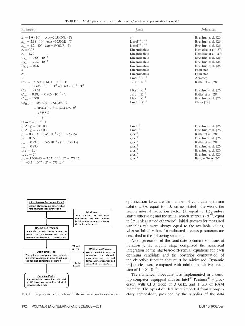
As the obtained optimum solution must satisfy the pro-

cess model, as described in Eqs. 1–52, the sequential optimi-

zation procedure was implemented as recommended in the

literature and presented in Fig. 1 [38]. According to the se-

quential optimization procedure, the first stage corresponded

to the optimization task, when optimum candidates were

generated. According to the Monte Carlo procedure, the can-

didate optimum solutions of the estimation problem must be

obtained by generating random numbers in the form

xjð Þ

i;k ¼ xj�1ð Þi;k þ r

ðjÞi;kD

ðjÞi i ¼ 1; :::;m k ¼ 1; :::; n ð56Þ

where rðjÞi;k are pseudorandom numbers uniformly distributed

in the interval (�1, 1) and DðjÞi defines a search interval for

variable i at iteration j. Convergence can be achieved by

reducing the search interval along the iterative procedure in

the form

DðjÞi ¼ Dðj�1Þ

i

li ¼ 1; :::;m (57)

where l is a real number greater than 1. The numerical pa-

rameters that must be defined for implementation of the


optimization tasks are the number of candidate optimum

solutions (n, equal to 10, unless stated otherwise), the

search interval reduction factor (l, equal to 1.5, unless

stated otherwise) and the initial search intervals (Dð0Þi , equal

to 3si, unless stated otherwise). Initial guesses for measured

variables xð0Þi;k were always equal to the available values,

whereas initial values for estimated process parameters are

described in the following sections.

After generation of the candidate optimum solutions at

iteration j, the second stage comprised the numerical

integration of the algebraic-differential equations for each

optimum candidate and the posterior computation of

the objective function that must be minimized. Dynamic

trajectories were computed with minimum relative preci-

sion of 1.0 3 1026.

The numerical procedure was implemented in a desk-

top computer, equipped with an Intel1 Pentium1 4 proc-

essor, with CPU clock of 3 GHz, and 1 GB of RAM

memory. The operation data were imported from a propri-

etary spreadsheet, provided by the supplier of the dataFIG. 1. Proposed numerical scheme for the in-line parameter estimation.

TABLE 1. Model parameters used in the styrene/butadiene copolymerization model.

Parameters Units References

kd ¼ 1.0 � 1022 � cxp(2205000/R � T) s21 Brandrup et al. [26]

kp11 ¼ 2.16 � 107 � exp(232500/R � T) L mol21 s21 Brandrup et al. [26]

kp22 ¼ 1.2 � 107 � exp(239000/R � T) L mol21 s21 Brandrup et al. [26]

r1 ¼ 0.78 Dimensionless Hamielec et al. [27]

r2 ¼ 1.39 Dimensionless Hamielec et al. [27]

CtrM11¼ 0.65 � 1024 Dimensionless Brandrup et al. [26]

CtrM22¼ 2.32 � 1024 Dimensionless Brandrup et al. [26]

CtrATC¼ 0.66 Dimensionless Brandrup et al. [26]

n Dimensionless Estimated

NT Dimensionless Estimated

R J mol21 K21 Admitted

Cp1 ¼ 26.747 þ 1471 � 1021 � T29.609 � 1025 � T2 – 2.373 � 1028 � T3

cal g21 K21 Kalfas et al. [28]

Cp2 ¼ 123.60 J Kg21 K21 Brandrup et al. [26]

Cp}1¼ 0.283 2 0.966 � 1023 � T cal g21 K21 Kalfas et al. [28]

Cp}2¼ 1600 J Kg21 K21 Brandrup et al. [26]

CpH2O¼ �203:606þ 1523:290 � h

� 3196:413 � h2 þ 2474:455 � h3

þ 3:855532

h2

Com y ¼ 1023 � T

J mol21 K21 Chase [29]

(2DH1) ¼ 68500.0 J mol21 Brandrup et al. [26]

(2DH2) ¼ 73000.0 J mol21 Brandrup et al. [26]

q1 ¼ 0.9193 2 6.65�1024 � (T 2 273.15) g cm3 Kalfas et al. [28]

q2 ¼ 0.650 g cm3 Brandrup et al. [26]

q}1¼ 0.9926 2 2.65�1024 � (T 2 273.15) g cm3 Kalfas et al. [28]

q}2¼ 0.890 g cm3 Brandrup et al. [26]

qInic ¼ 2.5 g cm3 Brandrup et al. [26]

qCTA ¼ 2.1 g cm3 Brandrup et al. [26]

qw ¼ 1.000663 2 7.35�1025 � (T 2 273.15)

23.5 � 1026 � (T 2 273.15)2g cm3 Perry e Green [30]


acquisition system, and stored as text input files for poste-

rior manipulation of the FORTRAN code. Similarly,

estimated monomer conversion, solids content, and copol-

ymer composition were exported to the data acquisition

spreadsheet for posterior analysis and manipulation.

Unless stated otherwise, sampling times of 5 min were

used for estimation of model parameters and states, taking

less than 2 min for the optimization task to be finished.

RESULTS AND DISCUSSION

Model Validation

First, the process model was validated with experimen-

tal datasets obtained from polymerization reactions carried

out in a small Pilot-plant reactor (3 l) and in a full-scale

industrial plant. Detailed description of reactor geometry

and of polymerization recipe is not provided for proprie-

tary reasons.

Temperature and Pressure Profiles in the Industrial Plant

For validation of model performance in the industrial

process, available jacket temperatures and polymerization

recipes were used as inputs to calculate pressure and tem-

perature profiles, which were then compared to available

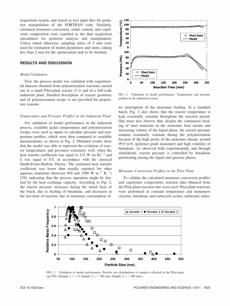
measurements, as shown in Fig. 2. Obtained results show

that the model was able to represent the evolution of reac-

tor temperatures and pressures extremely well, when the

heat transfer coefficient was equal to 214 W (m K)21 and

n was equal to 0.5, in accordance with the classical

Smith-Ewart-Harkins Theory. The estimated heat transfer

coefficient was lower than usually reported for other

aqueous emulsions (between 850 and 1500 W m21 K21)

[39], indicating that the process operation might be lim-

ited by the heat exchange capacity. According to Fig. 2,

the reactor pressure increases during the initial hour of

the batch, due to feeding of butadiene, and decreases in

the last hour of reaction, due to monomer consumption af-

ter interruption of the monomer feeding. In a standard

batch, Fig. 2 also shows that the reactor temperature is

kept essentially constant throughout the reaction period.

One must also observe that, despite the continuous feed-

ing of inert materials in the monomer feed stream and

increasing volume of the liquid phase, the reactor pressure

remains essentially constant during the polymerization

because of the high purity of the monomer stream, around

99.9 wt% (polymer grade monomer) and high volatility of

butadiene. As observed both experimentally and through

simulations, reactor pressure is controlled by butadiene

partitioning among the liquid and gaseous phases.

Monomer Conversion Profiles in the Pilot Plant

To validate the calculated monomer conversion profiles

and copolymer composition, reaction data obtained from

the Pilot-plant reaction runs were used. Pilot plant reactions

were performed at constant temperature and monomers

(styrene, butadiene, and carboxylic acids), surfactant, initia-

FIG. 2. Validation of model performance. Temperature and pressure

profiles in the industrial reactor.

FIG. 3. Validation of model performance. Particle size distributions of samples collected in the Pilot-plant

run P40. (Sample 1, t ¼ 0; Sample 2, t ¼ 200 min; Sample 3, t ¼ 400 min.)


tor (ammonium persulfate, APS) and water were fed at con-

stant flow rates for a period of 240 min. After that, a second

stream of initiator was fed into the system for an additional

period of 30 min.

Initially, as the emulsion polymerizations were seeded

and the classical n value was found to be equal to 0.5 in the

previous validation test, the parameter (n � NT) was esti-

mated as a constant value for the whole Pilot-plant poly-

merization runs. However, obtained results were not good.

As shown in Fig. 3, the particle size distribution (measured

offline with the help of a Brookhaven ultracentrifuge) was

shifted toward higher particle diameters during the course

of the polymerization, but average particle sizes did not

change significantly between the beginning and the end of

the run (about two times, whereas the polymer mass

increased about 20 times), indicating that particle nuclea-

tion took place during the batch. Although this experimen-

tal result contradicts one of the assumptions used to

build the mathematical model, the fact is that the parameter

(n � NT) can be estimated with the available data as a func-

tion of the reaction time without having to model the nucle-

ation step and significantly increasing the model size.

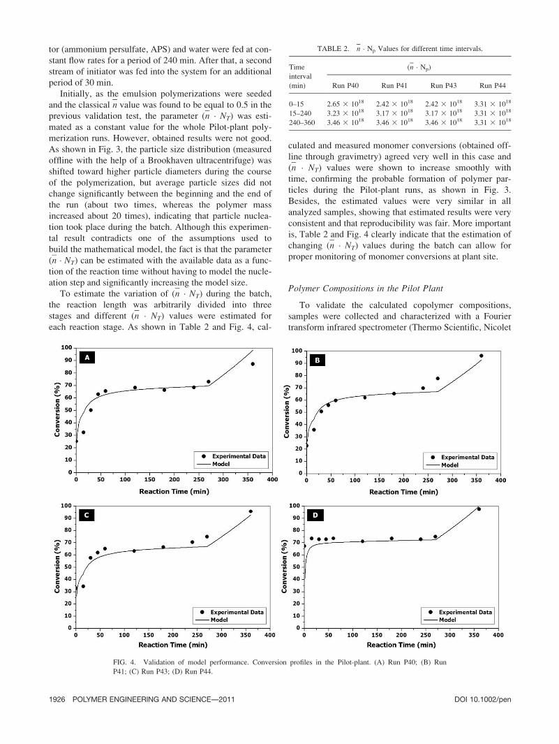
To estimate the variation of (n � NT) during the batch,

the reaction length was arbitrarily divided into three

stages and different (n � NT) values were estimated for

each reaction stage. As shown in Table 2 and Fig. 4, cal-

culated and measured monomer conversions (obtained off-

line through gravimetry) agreed very well in this case and

(n � NT) values were shown to increase smoothly with

time, confirming the probable formation of polymer par-

ticles during the Pilot-plant runs, as shown in Fig. 3.

Besides, the estimated values were very similar in all

analyzed samples, showing that estimated results were very

consistent and that reproducibility was fair. More important

is, Table 2 and Fig. 4 clearly indicate that the estimation of

changing (n � NT) values during the batch can allow for

proper monitoring of monomer conversions at plant site.

Polymer Compositions in the Pilot Plant

To validate the calculated copolymer compositions,

samples were collected and characterized with a Fourier

transform infrared spectrometer (Thermo Scientific, Nicolet

TABLE 2. n � Np Values for different time intervals.

Time

interval

(min)

(n � Np)

Run P40 Run P41 Run P43 Run P44

0–15 2.65 3 1018 2.42 3 1018 2.42 3 1018 3.31 3 1018

15–240 3.23 3 1018 3.17 3 1018 3.17 3 1018 3.31 3 1018

240–360 3.46 3 1018 3.46 3 1018 3.46 3 1018 3.31 3 1018

FIG. 4. Validation of model performance. Conversion profiles in the Pilot-plant. (A) Run P40; (B) Run

P41; (C) Run P43; (D) Run P44.


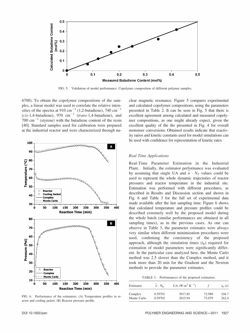
6700). To obtain the copolymer compositions of the sam-

ples, a linear model was used to correlate the relative inten-

sities of the spectra at 910 cm21 (1,2-butadiene), 740 cm21

(cis-1,4-butadiene), 970 cm21 (trans-1,4-butadiene), and

700 cm21 (styrene) with the butadiene content of the resin

[40]. Standard samples used for calibration were prepared

at the industrial reactor and were characterized through nu-

clear magnetic resonance. Figure 5 compares experimental

and calculated copolymer compositions, using the parameters

presented in Table 2. It can be seen in Fig. 5 that there is

excellent agreement among calculated and measured copoly-

mer compositions, as one might already expect, given the

excellent quality of the fits presented in Fig. 4 for overall

monomer conversions. Obtained results indicate that reactiv-

ity ratios and kinetic constants used for model simulations can

be used with confidence for representation of kinetic rates.

Real Time Applications

Real-Time Parameter Estimation in the Industrial

Plant. Initially, the estimator performance was evaluated

by assuming that single UA and n � NT values could be

used to represent the whole dynamic trajectories of reactor

pressures and reactor temperature in the industrial site.

Estimation was performed with different procedures, as

described in Results and Discussion section and shown in

Fig. 6 and Table 3 for the full set of experimental data

made available after the last sampling time. Figure 6 shows

that calculated temperature and pressure profiles could be

described extremely well by the proposed model during

the whole batch (similar performances are obtained in all

sampling times), as in the previous cases. As one can

observe in Table 3, the parameter estimates were always

very similar when different minimization procedures were

used, confirming the consistency of the proposed

approach, although the simulation times (tE) required for

estimation of model parameters were significantly differ-

ent. In the particular case analyzed here, the Monte Carlo

method was 2.5 slower than the Complex method, and it

took more than 20 min for the Gradient and the Newton

methods to provide the parameter estimates.

FIG. 6. Performance of the estimators. (A) Temperature profiles in re-

actor and cooling jacket; (B) Reactor pressure profile.

FIG. 5. Validation of model performance. Copolymer composition of different polymer samples.

TABLE 3. Performances of the proposed estimators.

Estimator n � Np UA (W�m2 K21) f tE (s)

Complex 0.59701 3017.85 72.988 104.7

Monte Carlo 0.59702 3015.94 73.079 262.4


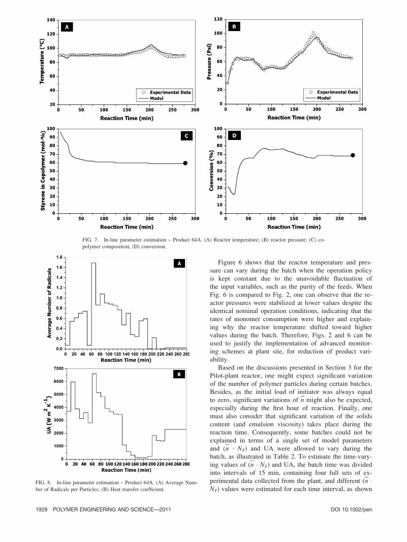
Figure 6 shows that the reactor temperature and pres-

sure can vary during the batch when the operation policy

is kept constant due to the unavoidable fluctuation of

the input variables, such as the purity of the feeds. When

Fig. 6 is compared to Fig. 2, one can observe that the re-

actor pressures were stabilized at lower values despite the

identical nominal operation conditions, indicating that the

rates of monomer consumption were higher and explain-

ing why the reactor temperature shifted toward higher

values during the batch. Therefore, Figs. 2 and 6 can be

used to justify the implementation of advanced monitor-

ing schemes at plant site, for reduction of product vari-

ability.

Based on the discussions presented in Section 3 for the

Pilot-plant reactor, one might expect significant variation

of the number of polymer particles during certain batches.

Besides, as the initial load of initiator was always equal

to zero, significant variations of n might also be expected,

especially during the first hour of reaction. Finally, one

must also consider that significant variation of the solids

content (and emulsion viscosity) takes place during the

reaction time. Consequently, some batches could not be

explained in terms of a single set of model parameters

and (n � NT) and UA were allowed to vary during the

batch, as illustrated in Table 2. To estimate the time-vary-

ing values of (n � NT) and UA, the batch time was divided

into intervals of 15 min, containing four full sets of ex-

perimental data collected from the plant, and different (n �NT) values were estimated for each time interval, as shown

FIG. 7. In-line parameter estimation – Product 64A. (A) Reactor temperature; (B) reactor pressure; (C) co-

polymer composition; (D) conversion.

FIG. 8. In-line parameter estimation – Product 64A. (A) Average Num-

ber of Radicals per Particles; (B) Heat transfer coefficient.


in Figs. 7 and 8. (The use of Kalman filters was avoided to

avoid the increase of the system dimension and the manipu-

lation and inversion of matrixes of derivatives.)

Figures 7 and 8 show that the parameter estimates can

change quite significantly during some batches, as already

explained, allowing for proper representation of reactor

temperature and pressure trajectories. Particularly, Fig. 7A

and B show that the reactor operation was driven to run-

away operation conditions, probably due to the uncon-

trolled increase of particle nucleation, followed afterward

by particle coagulation. In the analyzed case, feeding of

organic and aqueous streams was kept constant during the

first 200 min of operation and was halted after runaway

for safety reasons (therefore, normal operation was inter-

rupted after 200 min). Particle nucleation can justify the

continuous increase of (n � NT) during the first part of the

batch (represented in terms of n, when NT is assumed

constant and equal to the initial particle seed concentra-

tion), whereas particle coagulation can justify the steep

decrease of n � NT and UA during the second part of the

run. Despite that, it is important to note that the n values

shown in Fig. 8 are also consistent with experimental

results reported by Abdollahi and Sharifpour [41], as

these authors showed that n can be significantly influ-

enced by the nature of the carboxylic acid used in XSBR

emulsion polymerizations and can range from 0.3 to 1.7

in presence of acrylic, methacrylic, and itaconic acids.

Figure 7C and D illustrate how important the imple-

mentation of soft sensors can be at plant site, as there

were clear indications of dangerous monomer accumula-

tion inside the reactor during the first hour of reaction,

given the very low estimated monomer conversions in the

first part of the run, before the sudden increase of n � NT.

If estimated conversion data are compared to the mono-

mer solubility in the polymer particles (ranging from 39

to 40 wt%), it can clearly be concluded that formation of

monomer droplets takes place, as predicted by the pro-

posed polymerization model. Figure 7C also illustrates the

very significant drift of the copolymer composition during

the first reaction stage, as butadiene was accumulated pri-

marily in the gas phase. Both pieces of information could

be used for posterior optimization of the operation proce-

dure.

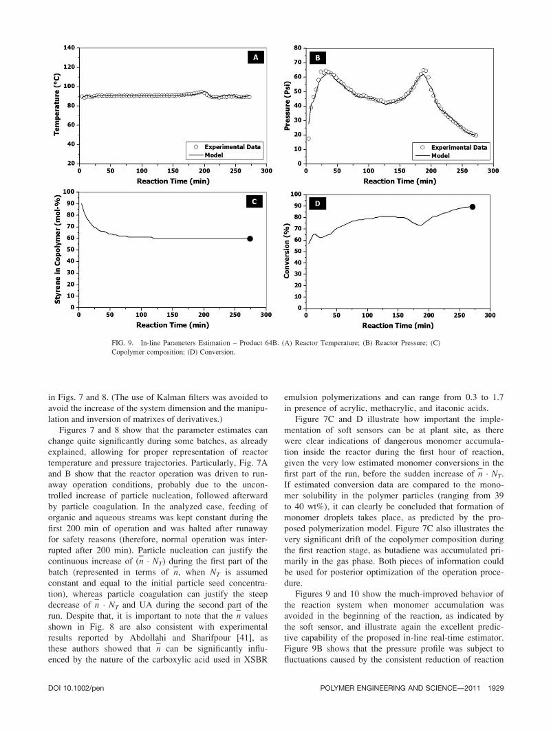
Figures 9 and 10 show the much-improved behavior of

the reaction system when monomer accumulation was

avoided in the beginning of the reaction, as indicated by

the soft sensor, and illustrate again the excellent predic-

tive capability of the proposed in-line real-time estimator.

Figure 9B shows that the pressure profile was subject to

fluctuations caused by the consistent reduction of reaction

FIG. 9. In-line Parameters Estimation – Product 64B. (A) Reactor Temperature; (B) Reactor Pressure; (C)

Copolymer composition; (D) Conversion.


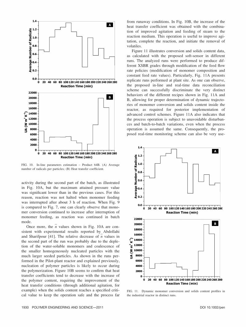
activity during the second part of the batch, as illustrated

in Fig. 10A, but the maximum attained pressure value

was significant lower than in the previous cases. For this

reason, reaction was not halted when monomer feeding

was interrupted after about 3 h of reaction. When Fig. 9

is compared to Fig. 7, one can clearly observe that mono-

mer conversion continued to increase after interruption of

monomer feeding, as reaction was continued in batch

mode.

Once more, the n values shown in Fig. 10A are con-

sistent with experimental results reported by Abdollahi

and Sharifpour [41]. The relative decrease of n values in

the second part of the run was probably due to the deple-

tion of the water-soluble monomers and coalescence of

the smaller homogeneously nucleated particles with the

much larger seeded particles. As shown in the runs per-

formed in the Pilot-plant reactor and explained previously,

nucleation of polymer particles is likely to occur during

the polymerization. Figure 10B seems to confirm that heat

transfer coefficients tend to decrease with the increase of

the polymer content, requiring the improvement of the

heat transfer conditions (through additional agitation, for

example) when the solids content reaches a specified criti-

cal value to keep the operation safe and the process far

from runaway conditions. In Fig. 10B, the increase of the

heat transfer coefficient was obtained with the combina-

tion of improved agitation and feeding of steam to the

reaction medium. This operation is useful to improve agi-

tation, complete the reaction, and initiate the removal of

volatiles.

Figure 11 illustrates conversion and solids content data,

as calculated with the proposed soft-sensor in different

runs. The analyzed runs were performed to produce dif-

ferent XSBR grades through modification of the feed flow

rate policies (modification of monomer composition and

constant feed rate values). Particularly, Fig. 11A presents

replicate runs performed at plant site. As one can observe,

the proposed in-line and real-time data reconciliation

scheme can successfully discriminate the very distinct

behaviors of the different recipes shown in Fig. 11A and

B, allowing for proper determination of dynamic trajecto-

ries of monomer conversion and solids content inside the

reactor, as required for posterior implementation of

advanced control schemes. Figure 11A also indicates that

the process operation is subject to unavoidable disturban-

ces and batch-to-batch variations, even when the process

operation is assumed the same. Consequently, the pro-

posed real-time monitoring scheme can also be very use-

FIG. 11. Dynamic monomer conversion and solids content profiles in

the industrial reactor in distinct runs.

FIG. 10. In-line parameters estimation – Product 64B. (A) Average

number of radicals per particles; (B) Heat transfer coefficient.


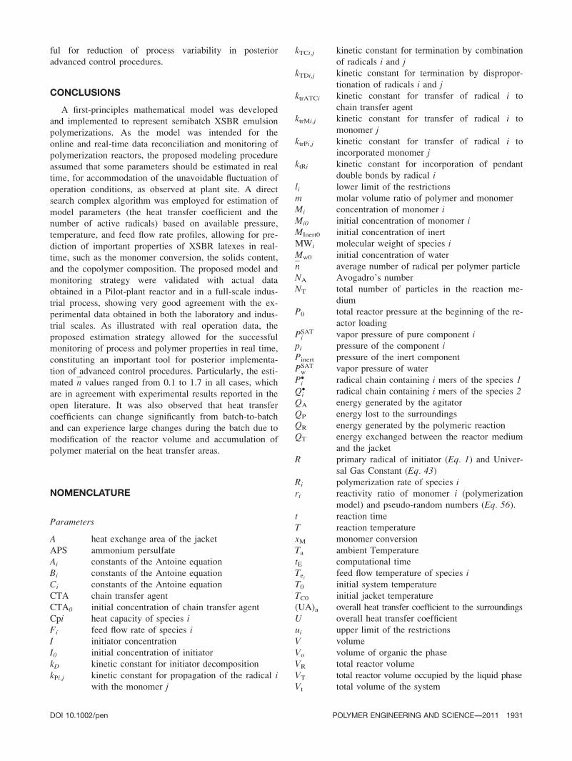
ful for reduction of process variability in posterior

advanced control procedures.

CONCLUSIONS

A first-principles mathematical model was developed

and implemented to represent semibatch XSBR emulsion

polymerizations. As the model was intended for the

online and real-time data reconciliation and monitoring of

polymerization reactors, the proposed modeling procedure

assumed that some parameters should be estimated in real

time, for accommodation of the unavoidable fluctuation of

operation conditions, as observed at plant site. A direct

search complex algorithm was employed for estimation of

model parameters (the heat transfer coefficient and the

number of active radicals) based on available pressure,

temperature, and feed flow rate profiles, allowing for pre-

diction of important properties of XSBR latexes in real-

time, such as the monomer conversion, the solids content,

and the copolymer composition. The proposed model and

monitoring strategy were validated with actual data

obtained in a Pilot-plant reactor and in a full-scale indus-

trial process, showing very good agreement with the ex-

perimental data obtained in both the laboratory and indus-

trial scales. As illustrated with real operation data, the

proposed estimation strategy allowed for the successful

monitoring of process and polymer properties in real time,

constituting an important tool for posterior implementa-

tion of advanced control procedures. Particularly, the esti-

mated n values ranged from 0.1 to 1.7 in all cases, which

are in agreement with experimental results reported in the

open literature. It was also observed that heat transfer

coefficients can change significantly from batch-to-batch

and can experience large changes during the batch due to

modification of the reactor volume and accumulation of

polymer material on the heat transfer areas.

NOMENCLATURE

Parameters

A heat exchange area of the jacket

APS ammonium persulfate

Ai constants of the Antoine equation

Bi constants of the Antoine equation

Ci constants of the Antoine equation

CTA chain transfer agent

CTA0 initial concentration of chain transfer agent

Cpi heat capacity of species iFi feed flow rate of species iI initiator concentration

I0 initial concentration of initiator

kD kinetic constant for initiator decomposition

kPi,j kinetic constant for propagation of the radical iwith the monomer j

kTCi,j kinetic constant for termination by combination

of radicals i and jkTDi,j kinetic constant for termination by dispropor-

tionation of radicals i and jktrATCi kinetic constant for transfer of radical i to

chain transfer agent

ktrMi,j kinetic constant for transfer of radical i to

monomer jktrPi,j kinetic constant for transfer of radical i to

incorporated monomer jktRi kinetic constant for incorporation of pendant

double bonds by radical ili lower limit of the restrictions

m molar volume ratio of polymer and monomer

Mi concentration of monomer iMi0 initial concentration of monomer iMInert0 initial concentration of inert

MWi molecular weight of species iMw0 initial concentration of water

n average number of radical per polymer particle

NA Avogadro’s number

NT total number of particles in the reaction me-

dium

P0 total reactor pressure at the beginning of the re-

actor loading

PSATi vapor pressure of pure component i

pi pressure of the component iPinert pressure of the inert component

PSATw vapor pressure of water

P�i radical chain containing i mers of the species 1

Q�i radical chain containing i mers of the species 2

QA energy generated by the agitator

QP energy lost to the surroundings

QR energy generated by the polymeric reaction

QT energy exchanged between the reactor medium

and the jacket

R primary radical of initiator (Eq. 1) and Univer-

sal Gas Constant (Eq. 43)Ri polymerization rate of species iri reactivity ratio of monomer i (polymerization

model) and pseudo-random numbers (Eq. 56).t reaction time

T reaction temperature

xM monomer conversion

Ta ambient Temperature

tE computational time

Tei feed flow temperature of species iT0 initial system temperature

TC0 initial jacket temperature

(UA)a overall heat transfer coefficient to the surroundings

U overall heat transfer coefficient

ui upper limit of the restrictions

V volume

Vo volume of organic the phase

VR total reactor volume

VT total reactor volume occupied by the liquid phase

Vt total volume of the system


Vw volume of aqueous phase

xi independent variables

xM monomers conversion

xS solid content

wi mass fraction of component iwInert molar fraction of volatile impurities (inert) in

the butadiene stream

Greek Symbols

I copolymer composition

/i volume fraction of component iGk dead polymer chain containing k mers

}i concentration of polymer i}i0 initial concentration of polymer iRk radical of polymer containing k mers

Oi probability of radicals in the polymer particle

present a mer of type i at the end of the polymer

chain

mi molar volume of component ipi pure density of species iv Flory–Huggins interaction parameter

(2DHi) enthalpy of homopolymerization of species i

Subscripts

1 styrene

2 butadiene

REFERENCES

1. T. Cosse. ‘‘Structural Changes in the Global Carboxylated

Styrene-Butadiene Latex Industry,’’ in International LatexConference, Rubber & Plastics News, Akron, USA (2003).

2. D.C. Blackley, Emulsion Polymerization: Theory and Prac-tice, Springer, New York (1975).

3. R.B. Gilbert, Emulsion Polymerization: A MechanisticApproach, Academic Press, London (1995).

4. J.C. Daniel and C. Pichot, Les Latex Synthetiques, Tec &

Doc Lavoisier, Paris (2006).

5. P.A. Lovell and M.S. El-Aasser, Emulsion Polymerizationand Emulsion Polymers, Wiley, New York (1997).

6. L. Vorwerg and R.G. Gilbert,Macromolecules, 33, 6693 (2000).

7. J.Y.M. Chew, S.J. Tonneijk, W.R. Paterson, and D.I. Wil-

son, Ind. Eng. Chem. Res., 44, 4605 (2005).

8. J.S. Nettleton, M.J.G. Davidson, and H.L. Williams, Ind.Eng. Chem., 45, 1896 (1953).

9. J.R. Leiza and J.C. Pinto, ‘‘Control of Polymerization Reac-

tors,’’ in Polymer Reaction Engineering, J.M. Asua, Ed.

Blackwell Publishing, Oxford (2007).

10. J.M. de Faria Jr., F. Machado, E.L. Lima, and J.C. Pinto,

Macromol. React. Eng., 4, 11 (2010).

11. J.M. de Faria Jr., F. Machado, E.L. Lima, and J.C. Pinto,

Macromol. React. Eng., 4, 486 (2010).

12. I.S. De Buruaga, M. Arotcarena, P.D. Armitage, L.M. Gugliotta,

J.R. Leiza, and J.M. Asua, Chem. Eng. Sci., 51, 2781 (1996).

13. L.M. Gugliotta, M. Arotcarena, J.R. Leiza, and J.M. Asua,

Polymer, 36, 2019 (1995).

14. B. Alhamad, V.G. Gomes, and J.A. Romagnoli, Int. J.

Chem. Reac. Eng., 4, 1 (2006).

15. I.W. Cheong and J.H. Kimu, Coll. Surf. A: Physicochem.Eng. Asp., 153, 137 (1999).

16. M. Vicente, S. Benamor, L.M. Gugliotta, J.R. Leiza, and

J.M. Asua, Ind. Eng. Chem. Res., 40, 218 (2001).

17. M.F. Kemmere, J. Meuldijk, A.A.H. Drinkenburg, and A.L.

German, J. Appl. Polym. Sci., 79, 944 (2001).

18. F. Korber, K. Hauschild, and G. Fink, Macromol. Chem.

Phys., 202, 3329 (2001).

19. F. Korber, K. Hauschild, M. Winter, and G. Fink, Macro-

mol. Chem. Phys., 202, 3323 (2001).

20. G. Maschio, I. Ferrara, C. Bassani, and H. Nieman, Chem.

Eng. Sci., 54, 3273 (1999).

21. J.R. Vega, L.M. Gugliotta, and G.R. Meira, Polym. React.

Eng., 10, 59 (2002).

22. L.M. Gugliotta, M.C. Brandolini, J.R. Vega, E.O. Iturralde,

J.L. Azum, and G.R. Meira, Polym. React. Eng., 3, 201 (1995).

23. C. Sayer, E.L. Lima, and J.C. Pinto, Chem. Eng. Sci., 52,

341 (1997).

24. C.C. Chang, A.F. Halasa, J.W. Miller Jr., and W.L. Hsu,

Polym. Int., 33, 151 (1994).

25. IMSL STAT/LIBRARY User’s Manual, 1991, Version 2.0,

IMSL, Houston.

26. J. Brandup, E.H. Immergut, and E.A. Grulke, PolymerHandbook, 4 ed., Wiley, New York (1999).

27. A.E. Hamielec, J.F. Mcgregor, S. Webb, and T. Spychaj,

‘‘Thermal and Chemical Initiated Copolymerization of Styrene

Acrylic Acid at High Temperatures and Conversions in a Con-

tinuous Stirred Tank Reactor,’’ in Polymer Reaction Engineering,

K.H.G. Reichert, W., Eds., Huthig and Wepf: Basel, 185 (1986).

28. G. Kalfas, H. Yuan, and W.H. Ray, Ind. Eng. Chem. Res.,32, 1831 (1993).

29. M.W. Chase Jr., J. Phys. Chem. Ref. Data, 9, 1 (1998).

30. R.H. Perry and D.W. Green, Perry’s Chemical Engineers’

Handbook, 7th ed., McGraw-Hill, New York (1997).

31. B. Hesselbo and R.B. Stinchcombe, Phys. Rev. Lett., 74,2151 (1995).

32. N.J. Box, Comput. J., 8, 42 (1965).

33. E.S. Lee, Ind. Eng. Chem. Fund., 3, 373 (1964).

34. P.E. Gill, W. Murray, and M.H. Wright, Practical Optimiza-tion, Academic Press, New York (1982).

35. E.K.P. Chong and S.H. Zak, An Introduction to Optimiza-

tion, 2nd ed., Wiley, New York (2001).

36. D.M. Prata, M. Schwaab, E.L. Lima, and J.C. Pinto, Chem.

Eng. Sci., 64, 3953 (2009).

37. W.H. Swann, ‘‘Constrained Optimization by Direct Search,’’ in

Numerical Methods for Constrained Optimization, P.E. Gill and

W. Murray, Eds., Academic Press, New York, USA (1974).

38. F. Machado, E.L. Lima, and J.C. Pinto, Polym. Eng. Sci.,

50, 697 (2010).

39. F.P. Incropera and D.P. Dewitt, Fundamentos de Transferen-

cia de Calor e de Massa, LTC Editora, Rio de Janeiro (2003).

40. J.G. Ivaschenko, N.N. Karpova, and O.V. Fedotova, Chem.Comput. Simul. Butlerov Commun., 4, 21 (2001).

41. M. Abdollahi and M. Sharifpour, Polymer, 48, 2035 (2007).


Documents

Real-time monitoring and parameter estimation of the emulsion polymerization of carboxylated styrene/butadiene latexes