Embed Size (px)
Citation preview
Steps and traces∗JURRIAAN ROT, Institute for Computing and Information Sciences, RadboudUniversiteit, Nijmegen 6525 EC, The Netherlands.E-mail: [email protected]
BART JACOBS, Institute for Computing and Information Sciences, RadboudUniversiteit, Nijmegen 6525 EC, The Netherlands.
PAUL BLAIN LEVY, School of Computer Science, University of Birmingham,Birmingham B15 2TT, UK.
AbstractIn the theory of coalgebras, trace semantics can be defined in various distinct ways, including through algebraic logics,the Kleisli category of a monad or its Eilenberg–Moore category. This paper elaborates two new unifying ideas: (i)coalgebraic,draftrules trace semantics is naturally presented in terms of corecursive algebras, and (ii) all three approachesarise as instances of the same abstract setting. Our perspective puts the different approaches under a common roof and allowsto derive conditions under which some of them coincide.
Keywords: Coalgebra, trace semantics, corecursive algebras
1 Introduction
Traces are used in the semantics of state-based systems as a way of recording the consecutivebehaviour of a state in terms of sequences of observable (input and/or output) actions. Tracesemantics leads to, for instance, the notion of trace equivalence, which expresses that two statescannot be distinguished by only looking at their iterated in/output behaviour.
Trace semantics is a central topic of interest in the coalgebra community—and not only there, ofcourse. One of the key features of the area of coalgebra is that states and their coalgebras can beconsidered in different universes, formalized as categories. The break-through insight is that tracesemantics for a system in universe A can often be obtained by switching to a different universe B.More explicitly, where the (ordinary) behaviour of the system can be described via a final coalgebrain universe A, the trace behaviour arises by finality in the different universe B. Typically, thealternative universe B is a category of algebraic logics, the Kleisli category or the category ofEilenberg–Moore algebras, of a monad on universe A.
This paper elaborates two new unifying ideas.1. We observe that the trace map from the state space of a coalgebra to a carrier of traces is in all
three situations the unique ‘coalgebra-to-algebra’ map to a corecursive algebra [7] of traces.
∗ This is a revised and extended version of a paper which appeared in the proceedings of CMCS 2018 [21].
Vol. 31, No. 6, © The Author(s) 2021. Published by Oxford University Press.This is an Open Access article distributed under the terms of the Creative Commons Attribution License (http://creativecommons.org/licenses/by/4.0/), which permits unrestricted reuse, distribution, and reproduction in any medium,provided the original work is properly cited.Advance Access Publication on 23 August 2021 https://doi.org/10.1093/logcom/exab050
Dow
nloaded from https://academ
ic.oup.com/logcom
/article/31/6/1482/6355531 by guest on 01 June 2022
Steps and traces 1483
This differs from earlier work which tries to describe traces as final coalgebras. For us, it isquite natural to view languages as algebras, certainly when they consist of finite words/traces.
2. Next, these corecursive algebras, used as spaces of traces, all arise via a uniform construction,in a setting given by an adjunction together with a special natural transformation that we calla ‘step’. We heavily rely on a basic result saying that in this situation, the (lifting of the) rightadjoint preserves corecursive algebras, sending them from one universe to another. This is aknown result [6], but its fundamental role in trace semantics has not been recognized before.For an arbitrary coalgebra, there is then a unique map to the transferred corecursive algebra;this is the trace map that we are after.
The main contribution of this paper is the unifying step-based approach to coalgebraic tracesemantics: it is shown that three existing f lavours of trace semantics—logical, Eilenberg–Mooreand Kleisli—are all instances of our approach. Moreover, comparison results are given relatingtheses. We focus only on finite trace semantics and also exclude at this stage the ‘iteration’ basedapproaches, e.g. in [9, 10, 31, 38].
Outline. The paper is organized as follows. It starts in Section 1 with the abstract step-and-adjunction setting and the relevant definitions and results for corecursive algebras. In the nextthree sections, it is explained how this setting gives rise to trace semantics, by presenting theabove-mentioned three approaches to coalgebraic trace semantics in terms of steps and adjunctions:Eilenberg–Moore (Section 3), logical (Section 4) and Kleisli (Section 5). In each case, the relevantcorecursive algebra is described. These sections are illustrated with several examples. In Section 6,we study partial traces for coalgebras with input and output [5], as another instance of the step-and-adjunction setting, but it is helpful to express that setting in the language of bimodules, which we doin Appendix B.
The next section establishes a connection between the Eilenberg–Moore and the logical approach,between the Kleisli and logical approach and between the Kleisli and Eilenberg–Moore approach(Section 7). In Section 8, we show that our construction yields algebras that are not merelycorecursive but completely iterative, a stronger property that provides more general trace semantics.Finally, in Section 9, we provide some directions for future work.
Notation. In the context of an adjunction F � G, we shall use overline notation (−) for adjointtransposition. The unit and counit of an adjunction are, as usual, written as η and ε.
For an endofunctor H , we write Alg(H) for its algebra category and CoAlg(H) for its coalgebracategory. For a monad (T , η, μ) on C, we write EM(T) for the Eilenberg–Moore category and K�(T)
for the Kleisli category.We recall that any functor S : Sets → Sets has a unique strength st. We write st : S(X A) → S(X )A
for st(t)(a) = S(eva)(t), where eva = λf .f (a) : X A → X .
2 Coalgebraic semantics from a step
This section is about the construction of corecursive algebras and their use for semantics. The notionof corecursive algebra, studied in [7, 11] as the dual of Taylor’s notion of recursive coalgebra [12],is defined as follows.
DEFINITION 2.1Let H be an endofunctor on a category C.
Dow
nloaded from https://academ
ic.oup.com/logcom
/article/31/6/1482/6355531 by guest on 01 June 2022
1484 Steps and traces
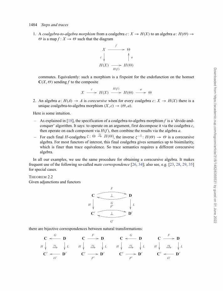
1. A coalgebra-to-algebra morphism from a coalgebra c : X → H(X ) to an algebra a : H(Θ) →Θ is a map f : X → Θ such that the diagram
commutes. Equivalently: such a morphism is a fixpoint for the endofunction on the homsetC(X , Θ) sending f to the composite
2. An algebra a : H(A) → A is corecursive when for every coalgebra c : X → H(X ) there is aunique coalgebra-to-algebra morphism (X , c) → (Θ , a).
Here is some intuition.
– As explained in [18], the specification of a coalgebra-to-algebra morphism f is a ‘divide-and-conquer’ algorithm. It says: to operate on an argument, first decompose it via the coalgebra c,then operate on each component via H(f ), then combine the results via the algebra a.
– For each final H-coalgebra , the inverse ζ−1 : H(Θ) → Θ is a corecursivealgebra. For most functors of interest, this final coalgebra gives semantics up to bisimilarity,which is finer than trace equivalence. So trace semantics requires a different corecursivealgebra.
In all our examples, we use the same procedure for obtaining a corecursive algebra. It makesfrequent use of the following so-called mate correspondence [26, 34]; also see, e.g. [23, 28, 29, 35]for special cases.
THEOREM 2.2Given adjunctions and functors
there are bijective correspondences between natural transformations:
Dow
nloaded from https://academ
ic.oup.com/logcom
/article/31/6/1482/6355531 by guest on 01 June 2022
Steps and traces 1485
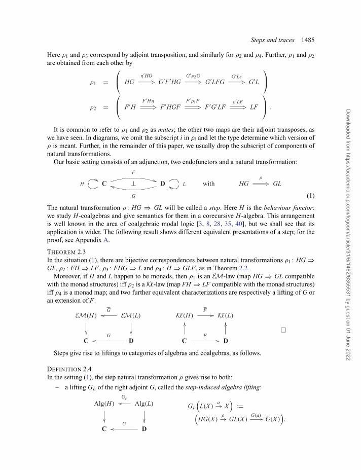
Here ρ1 and ρ3 correspond by adjoint transposition, and similarly for ρ2 and ρ4. Further, ρ1 and ρ2are obtained from each other by
It is common to refer to ρ1 and ρ2 as mates; the other two maps are their adjoint transposes, aswe have seen. In diagrams, we omit the subscript i in ρi and let the type determine which version ofρ is meant. Further, in the remainder of this paper, we usually drop the subscript of components ofnatural transformations.
Our basic setting consists of an adjunction, two endofunctors and a natural transformation:
(1)
The natural transformation ρ : HG ⇒ GL will be called a step. Here H is the behaviour functor:we study H-coalgebras and give semantics for them in a corecursive H-algebra. This arrangementis well known in the area of coalgebraic modal logic [3, 8, 28, 35, 40], but we shall see that itsapplication is wider. The following result shows different equivalent presentations of a step; for theproof, see Appendix A.
THEOREM 2.3In the situation (1), there are bijective correspondences between natural transformations ρ1 : HG ⇒GL, ρ2 : FH ⇒ LF, ρ3 : FHG ⇒ L and ρ4 : H ⇒ GLF, as in Theorem 2.2.
Moreover, if H and L happen to be monads, then ρ1 is an EM-law (map HG ⇒ GL compatiblewith the monad structures) iff ρ2 is a K�-law (map FH ⇒ LF compatible with the monad structures)iff ρ4 is a monad map; and two further equivalent characterizations are respectively a lifting of G oran extension of F:
Steps give rise to liftings to categories of algebras and coalgebras, as follows.
DEFINITION 2.4In the setting (1), the step natural transformation ρ gives rise to both:
– a lifting Gρ of the right adjoint G, called the step-induced algebra lifting:
Dow
nloaded from https://academ
ic.oup.com/logcom
/article/31/6/1482/6355531 by guest on 01 June 2022
1486 Steps and traces
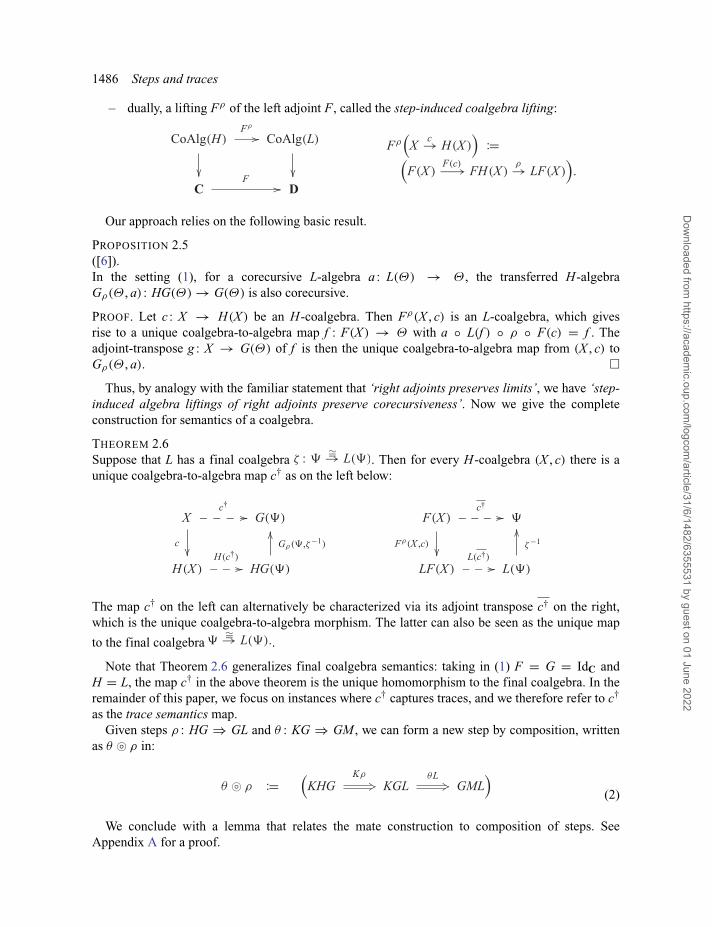
– dually, a lifting Fρ of the left adjoint F, called the step-induced coalgebra lifting:
Our approach relies on the following basic result.
PROPOSITION 2.5([6]).In the setting (1), for a corecursive L-algebra a : L(Θ) → Θ , the transferred H-algebraGρ(Θ , a) : HG(Θ) → G(Θ) is also corecursive.
PROOF. Let c : X → H(X ) be an H-coalgebra. Then Fρ(X , c) is an L-coalgebra, which givesrise to a unique coalgebra-to-algebra map f : F(X ) → Θ with a ◦ L(f ) ◦ ρ ◦ F(c) = f . Theadjoint-transpose g : X → G(Θ) of f is then the unique coalgebra-to-algebra map from (X , c) toGρ(Θ , a). �
Thus, by analogy with the familiar statement that ‘right adjoints preserves limits’, we have ‘step-induced algebra liftings of right adjoints preserve corecursiveness’. Now we give the completeconstruction for semantics of a coalgebra.
THEOREM 2.6Suppose that L has a final coalgebra . Then for every H-coalgebra (X , c) there is aunique coalgebra-to-algebra map c† as on the left below:
The map c† on the left can alternatively be characterized via its adjoint transpose c† on the right,which is the unique coalgebra-to-algebra morphism. The latter can also be seen as the unique map
to the final coalgebra .
Note that Theorem 2.6 generalizes final coalgebra semantics: taking in (1) F = G = IdC andH = L, the map c† in the above theorem is the unique homomorphism to the final coalgebra. In theremainder of this paper, we focus on instances where c† captures traces, and we therefore refer to c†
as the trace semantics map.Given steps ρ : HG ⇒ GL and θ : KG ⇒ GM , we can form a new step by composition, written
as θ � ρ in:
(2)
We conclude with a lemma that relates the mate construction to composition of steps. SeeAppendix A for a proof.
Dow
nloaded from https://academ
ic.oup.com/logcom
/article/31/6/1482/6355531 by guest on 01 June 2022
Steps and traces 1487
LEMMA 2.7Let ρ : HG ⇒ GL, θ : KG ⇒ GM be steps. Then
(θ � ρ
)2 = Mρ2 ◦ θ2H .
3 Traces via Eilenberg–Moore
We recall the approach to trace semantics developed in [4, 22, 43], putting it in the framework ofthe previous section. The approach deals with coalgebras for the composite functor BT , where T isa monad that captures the ‘branching’ aspect. The following assumptions are required.
ASSUMPTION 3.1(Traces via Eilenberg–Moore).In this section, we assume the following:
1. An endofunctor B : C → C with a final coalgebra .2. A monad (T , η, μ), with the standard adjunction F � U between categories C ←−−−−−−→ EM(T),
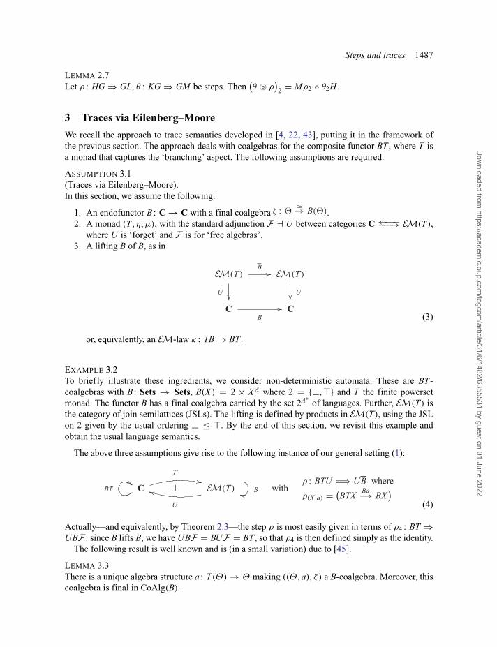
where U is ‘forget’ and F is for ‘free algebras’.3. A lifting B of B, as in
(3)
or, equivalently, an EM-law κ : TB ⇒ BT .
EXAMPLE 3.2To brief ly illustrate these ingredients, we consider non-deterministic automata. These are BT-coalgebras with B : Sets → Sets, B(X ) = 2 × X A where 2 = {⊥, } and T the finite powersetmonad. The functor B has a final coalgebra carried by the set 2A∗
of languages. Further, EM(T) isthe category of join semilattices (JSLs). The lifting is defined by products in EM(T), using the JSLon 2 given by the usual ordering ⊥ ≤ . By the end of this section, we revisit this example andobtain the usual language semantics.
The above three assumptions give rise to the following instance of our general setting (1):
(4)
Actually—and equivalently, by Theorem 2.3—the step ρ is most easily given in terms of ρ4 : BT ⇒UBF : since B lifts B, we have UBF = BUF = BT , so that ρ4 is then defined simply as the identity.
The following result is well known and is (in a small variation) due to [45].
LEMMA 3.3There is a unique algebra structure a : T(Θ) → Θ making ((Θ , a), ζ ) a B-coalgebra. Moreover, thiscoalgebra is final in CoAlg(B).
Dow
nloaded from https://academ
ic.oup.com/logcom
/article/31/6/1482/6355531 by guest on 01 June 2022
1488 Steps and traces
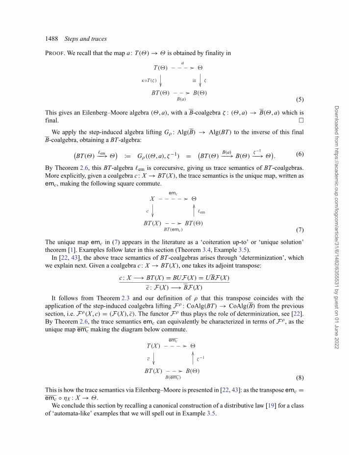
PROOF. We recall that the map a : T(Θ) → Θ is obtained by finality in
(5)
This gives an Eilenberg–Moore algebra (Θ , a), with a B-coalgebra ζ : (Θ , a) → B(Θ , a) which isfinal. �
We apply the step-induced algebra lifting Gρ : Alg(B) → Alg(BT) to the inverse of this finalB-coalgebra, obtaining a BT-algebra:(
BT(Θ)�em−−→ Θ
):= Gρ((Θ , a), ζ−1) = (
BT(Θ)B(a)−−→ B(Θ)
ζ−1
−−→ Θ). (6)
By Theorem 2.6, this BT-algebra �em is corecursive, giving us trace semantics of BT-coalgebras.More explicitly, given a coalgebra c : X → BT(X ), the trace semantics is the unique map, written asemc, making the following square commute.
(7)
The unique map emc in (7) appears in the literature as a ‘coiteration up-to’ or ‘unique solution’theorem [1]. Examples follow later in this section (Theorem 3.4, Example 3.5).
In [22, 43], the above trace semantics of BT-coalgebras arises through ‘determinization’, whichwe explain next. Given a coalgebra c : X → BT(X ), one takes its adjoint transpose:
c : X −→ BT(X ) = BUF(X ) = UBF(X )
c : F(X ) −→ BF(X )
It follows from Theorem 2.3 and our definition of ρ that this transpose coincides with theapplication of the step-induced coalgebra lifting Fρ : CoAlg(BT) → CoAlg(B) from the previoussection, i.e. Fρ(X , c) = (F(X ), c). The functor Fρ thus plays the role of determinization, see [22].By Theorem 2.6, the trace semantics emc can equivalently be characterized in terms of Fρ , as theunique map emc making the diagram below commute.
(8)
This is how the trace semantics via Eilenberg–Moore is presented in [22, 43]: as the transpose emc =emc ◦ ηX : X → Θ .
We conclude this section by recalling a canonical construction of a distributive law [19] for a classof ‘automata-like’ examples that we will spell out in Example 3.5.
Dow
nloaded from https://academ
ic.oup.com/logcom
/article/31/6/1482/6355531 by guest on 01 June 2022
Steps and traces 1489
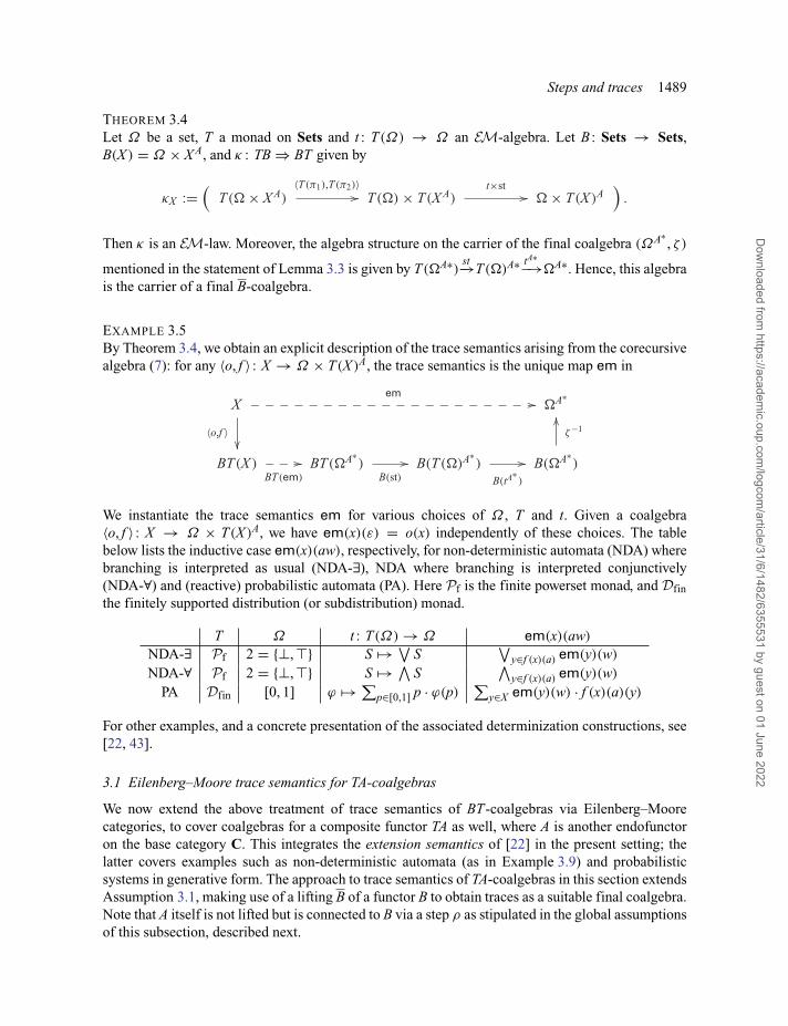
THEOREM 3.4Let Ω be a set, T a monad on Sets and t : T(Ω) → Ω an EM-algebra. Let B : Sets → Sets,B(X ) = Ω × X A, and κ : TB ⇒ BT given by
Then κ is an EM-law. Moreover, the algebra structure on the carrier of the final coalgebra (ΩA∗, ζ )
mentioned in the statement of Lemma 3.3 is given by T(�A∗) st−→T(�)A∗ tA∗−→�A∗. Hence, this algebrais the carrier of a final B-coalgebra.
EXAMPLE 3.5By Theorem 3.4, we obtain an explicit description of the trace semantics arising from the corecursivealgebra (7): for any 〈o, f 〉 : X → Ω × T(X )A, the trace semantics is the unique map em in
We instantiate the trace semantics em for various choices of Ω , T and t. Given a coalgebra〈o, f 〉 : X → Ω × T(X )A, we have em(x)(ε) = o(x) independently of these choices. The tablebelow lists the inductive case em(x)(aw), respectively, for non-deterministic automata (NDA) wherebranching is interpreted as usual (NDA-∃), NDA where branching is interpreted conjunctively(NDA-∀) and (reactive) probabilistic automata (PA). Here Pf is the finite powerset monad, and Dfinthe finitely supported distribution (or subdistribution) monad.
T Ω t : T(Ω) → Ω em(x)(aw)
NDA-∃ Pf 2 = {⊥, } S �→ ∨S
∨y∈f (x)(a) em(y)(w)
NDA-∀ Pf 2 = {⊥, } S �→ ∧S
∧y∈f (x)(a) em(y)(w)
PA Dfin [0, 1] ϕ �→ ∑p∈[0,1] p · ϕ(p)
∑y∈X em(y)(w) · f (x)(a)(y)
For other examples, and a concrete presentation of the associated determinization constructions, see[22, 43].
3.1 Eilenberg–Moore trace semantics for TA-coalgebras
We now extend the above treatment of trace semantics of BT-coalgebras via Eilenberg–Moorecategories, to cover coalgebras for a composite functor TA as well, where A is another endofunctoron the base category C. This integrates the extension semantics of [22] in the present setting; thelatter covers examples such as non-deterministic automata (as in Example 3.9) and probabilisticsystems in generative form. The approach to trace semantics of TA-coalgebras in this section extendsAssumption 3.1, making use of a lifting B of a functor B to obtain traces as a suitable final coalgebra.Note that A itself is not lifted but is connected to B via a step ρ as stipulated in the global assumptionsof this subsection, described next.
Dow
nloaded from https://academ
ic.oup.com/logcom
/article/31/6/1482/6355531 by guest on 01 June 2022
1490 Steps and traces
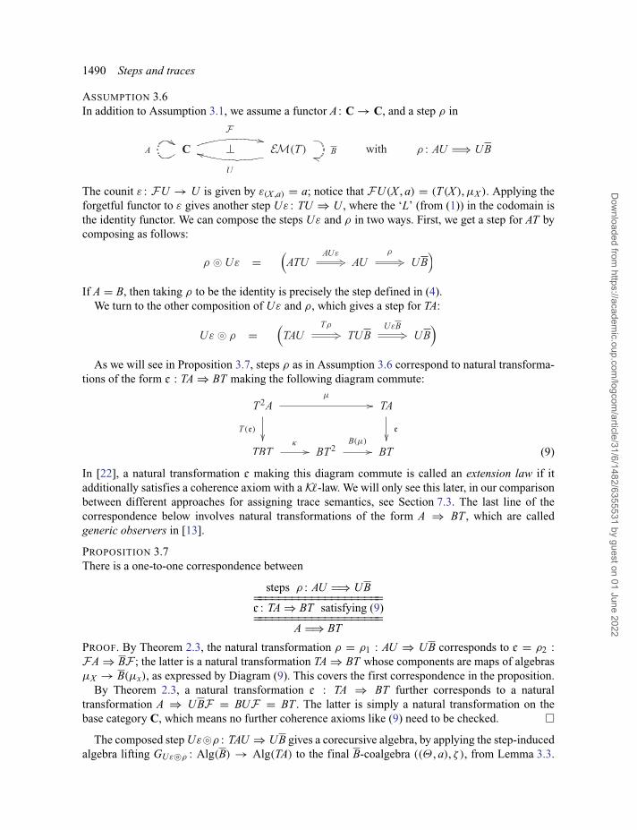
ASSUMPTION 3.6In addition to Assumption 3.1, we assume a functor A : C → C, and a step ρ in
The counit ε : FU → U is given by ε(X ,a) = a; notice that FU(X , a) = (T(X ), μX ). Applying theforgetful functor to ε gives another step Uε : TU ⇒ U , where the ‘L’ (from (1)) in the codomain isthe identity functor. We can compose the steps Uε and ρ in two ways. First, we get a step for AT bycomposing as follows:
If A = B, then taking ρ to be the identity is precisely the step defined in (4).We turn to the other composition of Uε and ρ, which gives a step for TA:
As we will see in Proposition 3.7, steps ρ as in Assumption 3.6 correspond to natural transforma-tions of the form e : TA ⇒ BT making the following diagram commute:
(9)
In [22], a natural transformation e making this diagram commute is called an extension law if itadditionally satisfies a coherence axiom with a K�-law. We will only see this later, in our comparisonbetween different approaches for assigning trace semantics, see Section 7.3. The last line of thecorrespondence below involves natural transformations of the form A ⇒ BT , which are calledgeneric observers in [13].
PROPOSITION 3.7There is a one-to-one correspondence between
steps ρ : AU �⇒ UB====================e : TA ⇒ BT satisfying (9)====================
A �⇒ BT
PROOF. By Theorem 2.3, the natural transformation ρ = ρ1 : AU ⇒ UB corresponds to e = ρ2 :FA ⇒ BF ; the latter is a natural transformation TA ⇒ BT whose components are maps of algebrasμX → B(μx), as expressed by Diagram (9). This covers the first correspondence in the proposition.
By Theorem 2.3, a natural transformation e : TA ⇒ BT further corresponds to a naturaltransformation A ⇒ UBF = BUF = BT . The latter is simply a natural transformation on thebase category C, which means no further coherence axioms like (9) need to be checked. �
The composed step Uε�ρ : TAU ⇒ UB gives a corecursive algebra, by applying the step-inducedalgebra lifting GUε�ρ : Alg(B) → Alg(TA) to the final B-coalgebra ((Θ , a), ζ ), from Lemma 3.3.
Dow
nloaded from https://academ
ic.oup.com/logcom
/article/31/6/1482/6355531 by guest on 01 June 2022
Steps and traces 1491
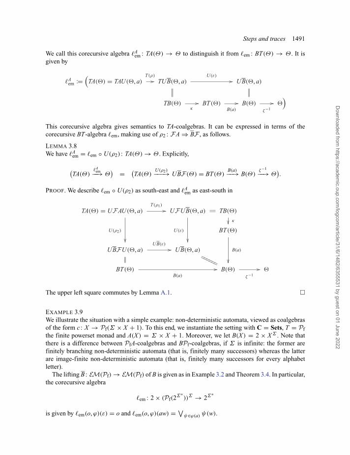
We call this corecursive algebra �Aem : TA(Θ) → Θ to distinguish it from �em : BT(Θ) → Θ . It is
given by
This corecursive algebra gives semantics to TA-coalgebras. It can be expressed in terms of thecorecursive BT-algebra �em, making use of ρ2 : FA ⇒ BF , as follows.
LEMMA 3.8We have �A
em = �em ◦ U(ρ2) : TA(Θ) → Θ . Explicitly,
(TA(Θ)
�Aem−−→ Θ
) = (TA(Θ)
U(ρ2)−−−→ UBF(Θ) = BT(Θ)B(a)−−→ B(Θ)
ζ−1
−−→ Θ).
PROOF. We describe �em ◦ U(ρ2) as south-east and �Aem as east-south in
The upper left square commutes by Lemma A.1. �
EXAMPLE 3.9We illustrate the situation with a simple example: non-deterministic automata, viewed as coalgebrasof the form c : X → Pf(Σ × X + 1). To this end, we instantiate the setting with C = Sets, T = Pfthe finite powerset monad and A(X ) = Σ × X + 1. Moreover, we let B(X ) = 2 × X Σ . Note thatthere is a difference between PfA-coalgebras and BPf-coalgebras, if Σ is infinite: the former arefinitely branching non-deterministic automata (that is, finitely many successors) whereas the latterare image-finite non-deterministic automata (that is, finitely many successors for every alphabetletter).
The lifting B : EM(Pf) → EM(Pf) of B is given as in Example 3.2 and Theorem 3.4. In particular,the corecursive algebra
�em : 2 × (Pf(2Σ∗))Σ → 2Σ∗
is given by �em(o, ϕ)(ε) = o and �em(o, ϕ)(aw) = ∨ψ∈ϕ(a) ψ(w).
Dow
nloaded from https://academ
ic.oup.com/logcom
/article/31/6/1482/6355531 by guest on 01 June 2022
1492 Steps and traces
The relevant step ρ : AU ⇒ UB is most easily given by ρ4 : A ⇒ UBF = BPf. On a componentX , we define (ρ4)X : Σ × X + 1 → 2 × (PfX )Σ by
(ρ4)X (a, x) =(
⊥, λb.
{{x} if a = b
∅ otherwise
), (ρ4)X (∗) = (, λb.∅) .
Then (ρ2)X : Pf(Σ × X + 1) → 2 × (PfX )Σ is the adjoint transpose, given by
ρ2(S) =(∨
∗∈S
, λa.{x | (a, x) ∈ S})
.
This coincides with the extension law given in [22].By Lemma 3.8, the corecursive PfA-algebra obtained from the final B-coalgebra is given by �A
em =�em ◦ U(ρ2) : Pf(Σ × 2Σ∗ + 1) → 2Σ∗
, which is
�Aem(S)(ε) =
∨∗∈S
, �Aem(S)(aw) =
∨(a,ψ)∈S
ψ(w) .
Given a coalgebra c : X → Pf(Σ × X + 1), the unique coalgebra-to-algebra morphismemA : X → 2Σ∗
from c to �Aem is thus given by emA(x)(ε) = ∨
∗∈c(x) and emA(x)(aw) =∨(a,y)∈c(x) emA(y)(w).
For examples of extension laws for weighted and probabilistic automata, see [22].
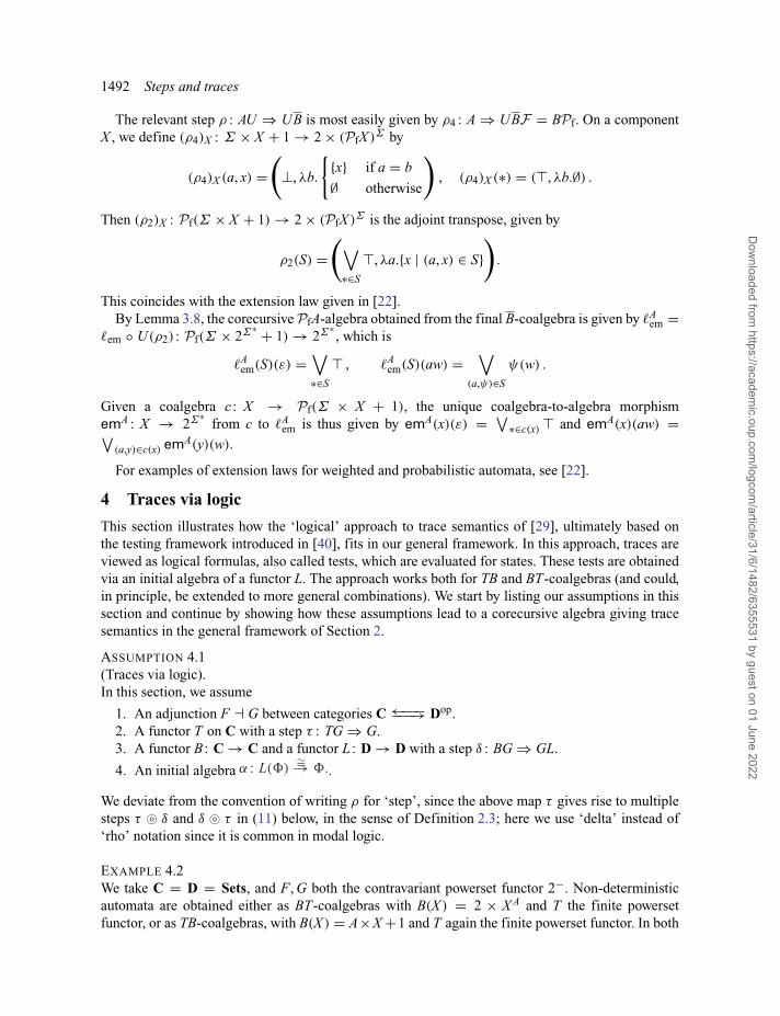
4 Traces via logic
This section illustrates how the ‘logical’ approach to trace semantics of [29], ultimately based onthe testing framework introduced in [40], fits in our general framework. In this approach, traces areviewed as logical formulas, also called tests, which are evaluated for states. These tests are obtainedvia an initial algebra of a functor L. The approach works both for TB and BT-coalgebras (and could,in principle, be extended to more general combinations). We start by listing our assumptions in thissection and continue by showing how these assumptions lead to a corecursive algebra giving tracesemantics in the general framework of Section 2.
ASSUMPTION 4.1(Traces via logic).In this section, we assume
1. An adjunction F � G between categories C ←−−−−−−→ Dop.2. A functor T on C with a step τ : TG ⇒ G.3. A functor B : C → C and a functor L : D → D with a step δ : BG ⇒ GL.
4. An initial algebra .
We deviate from the convention of writing ρ for ‘step’, since the above map τ gives rise to multiplesteps τ � δ and δ � τ in (11) below, in the sense of Definition 2.3; here we use ‘delta’ instead of‘rho’ notation since it is common in modal logic.
EXAMPLE 4.2We take C = D = Sets, and F, G both the contravariant powerset functor 2−. Non-deterministicautomata are obtained either as BT-coalgebras with B(X ) = 2 × X A and T the finite powersetfunctor, or as TB-coalgebras, with B(X ) = A×X +1 and T again the finite powerset functor. In both
Dow
nloaded from https://academ
ic.oup.com/logcom
/article/31/6/1482/6355531 by guest on 01 June 2022
Steps and traces 1493
cases, L is given by L(X ) = A × X + 1, which has the set of words A∗ as carrier of an initial algebra.The map τ : T2− ⇒ 2− is defined by τX (S)(x) = ∨
ϕ∈S ϕ(x) and intuitively models the existentialchoice in the semantics of non-deterministic automata. The step δ and the language semantics aredefined later in this section.
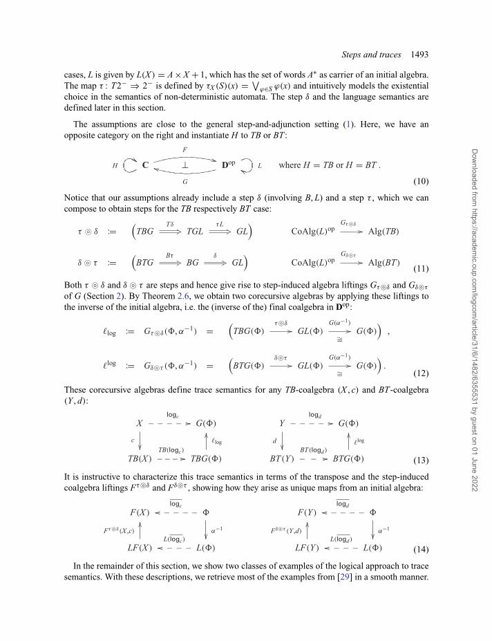
The assumptions are close to the general step-and-adjunction setting (1). Here, we have anopposite category on the right and instantiate H to TB or BT :
(10)
Notice that our assumptions already include a step δ (involving B, L) and a step τ , which we cancompose to obtain steps for the TB respectively BT case:
(11)
Both τ � δ and δ � τ are steps and hence give rise to step-induced algebra liftings Gτ�δ and Gδ�τ
of G (Section 2). By Theorem 2.6, we obtain two corecursive algebras by applying these liftings tothe inverse of the initial algebra, i.e. the (inverse of the) final coalgebra in Dop:
(12)
These corecursive algebras define trace semantics for any TB-coalgebra (X , c) and BT-coalgebra(Y , d):
(13)
It is instructive to characterize this trace semantics in terms of the transpose and the step-inducedcoalgebra liftings Fτ�δ and Fδ�τ , showing how they arise as unique maps from an initial algebra:
(14)
In the remainder of this section, we show two classes of examples of the logical approach to tracesemantics. With these descriptions, we retrieve most of the examples from [29] in a smooth manner.
Dow
nloaded from https://academ
ic.oup.com/logcom
/article/31/6/1482/6355531 by guest on 01 June 2022
1494 Steps and traces
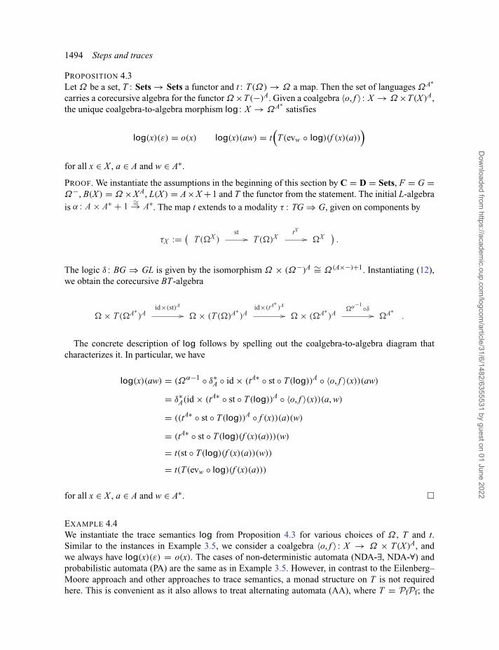
PROPOSITION 4.3Let Ω be a set, T : Sets → Sets a functor and t : T(Ω) → Ω a map. Then the set of languages ΩA∗
carries a corecursive algebra for the functor Ω ×T(−)A. Given a coalgebra 〈o, f 〉 : X → Ω ×T(X )A,the unique coalgebra-to-algebra morphism log : X → ΩA∗
satisfies
log(x)(ε) = o(x) log(x)(aw) = t(
T(evw ◦ log)(f (x)(a)))
for all x ∈ X , a ∈ A and w ∈ A∗.
PROOF. We instantiate the assumptions in the beginning of this section by C = D = Sets, F = G =Ω−, B(X ) = Ω ×X A, L(X ) = A×X +1 and T the functor from the statement. The initial L-algebra
is . The map t extends to a modality τ : TG ⇒ G, given on components by
The logic δ : BG ⇒ GL is given by the isomorphism Ω × (Ω−)A ∼= Ω(A×−)+1. Instantiating (12),we obtain the corecursive BT-algebra
The concrete description of log follows by spelling out the coalgebra-to-algebra diagram thatcharacterizes it. In particular, we have
log(x)(aw) = (Ωα−1 ◦ δ∗A ◦ id × (tA∗ ◦ st ◦ T(log))A ◦ 〈o, f 〉(x))(aw)
= δ∗A(id × (tA∗ ◦ st ◦ T(log))A ◦ 〈o, f 〉(x))(a, w)
= ((tA∗ ◦ st ◦ T(log))A ◦ f (x))(a)(w)
= (tA∗ ◦ st ◦ T(log)(f (x)(a)))(w)
= t(st ◦ T(log)(f (x)(a))(w))
= t(T(evw ◦ log)(f (x)(a)))
for all x ∈ X , a ∈ A and w ∈ A∗. �
EXAMPLE 4.4We instantiate the trace semantics log from Proposition 4.3 for various choices of Ω , T and t.Similar to the instances in Example 3.5, we consider a coalgebra 〈o, f 〉 : X → Ω × T(X )A, andwe always have log(x)(ε) = o(x). The cases of non-deterministic automata (NDA-∃, NDA-∀) andprobabilistic automata (PA) are the same as in Example 3.5. However, in contrast to the Eilenberg–Moore approach and other approaches to trace semantics, a monad structure on T is not requiredhere. This is convenient as it also allows to treat alternating automata (AA), where T = PfPf; the
Dow
nloaded from https://academ
ic.oup.com/logcom
/article/31/6/1482/6355531 by guest on 01 June 2022
Steps and traces 1495
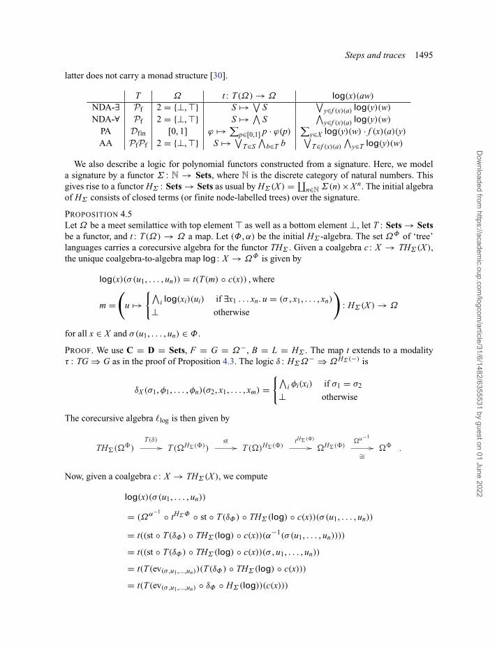
latter does not carry a monad structure [30].
T Ω t : T(Ω) → Ω log(x)(aw)
NDA-∃ Pf 2 = {⊥, } S �→ ∨S
∨y∈f (x)(a) log(y)(w)
NDA-∀ Pf 2 = {⊥, } S �→ ∧S
∧y∈f (x)(a) log(y)(w)
PA Dfin [0, 1] ϕ �→ ∑p∈[0,1] p · ϕ(p)
∑y∈X log(y)(w) · f (x)(a)(y)
AA PfPf 2 = {⊥, } S �→ ∨T∈S
∧b∈T b
∨T∈f (x)(a)
∧y∈T log(y)(w)
We also describe a logic for polynomial functors constructed from a signature. Here, we modela signature by a functor Σ : N → Sets, where N is the discrete category of natural numbers. Thisgives rise to a functor HΣ : Sets → Sets as usual by HΣ(X ) = ∐
n∈N Σ(n)×X n. The initial algebraof HΣ consists of closed terms (or finite node-labelled trees) over the signature.
PROPOSITION 4.5Let Ω be a meet semilattice with top element as well as a bottom element ⊥, let T : Sets → Setsbe a functor, and t : T(Ω) → Ω a map. Let (Φ, α) be the initial HΣ -algebra. The set ΩΦ of ‘tree’languages carries a corecursive algebra for the functor THΣ . Given a coalgebra c : X → THΣ(X ),the unique coalgebra-to-algebra map log : X → ΩΦ is given by
log(x)(σ (u1, . . . , un)) = t(T(m) ◦ c(x)) , where
m =(
u �→{∧
i log(xi)(ui) if ∃x1 . . . xn. u = (σ , x1, . . . , xn)
⊥ otherwise
): HΣ(X ) → Ω
for all x ∈ X and σ(u1, . . . , un) ∈ Φ.
PROOF. We use C = D = Sets, F = G = Ω−, B = L = HΣ . The map t extends to a modalityτ : TG ⇒ G as in the proof of Proposition 4.3. The logic δ : HΣΩ− ⇒ ΩHΣ(−) is
δX (σ1, φ1, . . . , φn)(σ2, x1, . . . , xm) ={∧
i φi(xi) if σ1 = σ2
⊥ otherwise
The corecursive algebra �log is then given by
Now, given a coalgebra c : X → THΣ(X ), we compute
log(x)(σ (u1, . . . , un))
= (Ωα−1 ◦ tHΣΦ ◦ st ◦ T(δΦ) ◦ THΣ(log) ◦ c(x))(σ (u1, . . . , un))
= t((st ◦ T(δΦ) ◦ THΣ(log) ◦ c(x))(α−1(σ (u1, . . . , un))))
= t((st ◦ T(δΦ) ◦ THΣ(log) ◦ c(x))(σ , u1, . . . , un))
= t(T(ev(σ ,u1,...,un))(T(δΦ) ◦ THΣ(log) ◦ c(x)))
= t(T(ev(σ ,u1,...,un) ◦ δΦ ◦ HΣ(log))(c(x)))
Dow
nloaded from https://academ
ic.oup.com/logcom
/article/31/6/1482/6355531 by guest on 01 June 2022
1496 Steps and traces
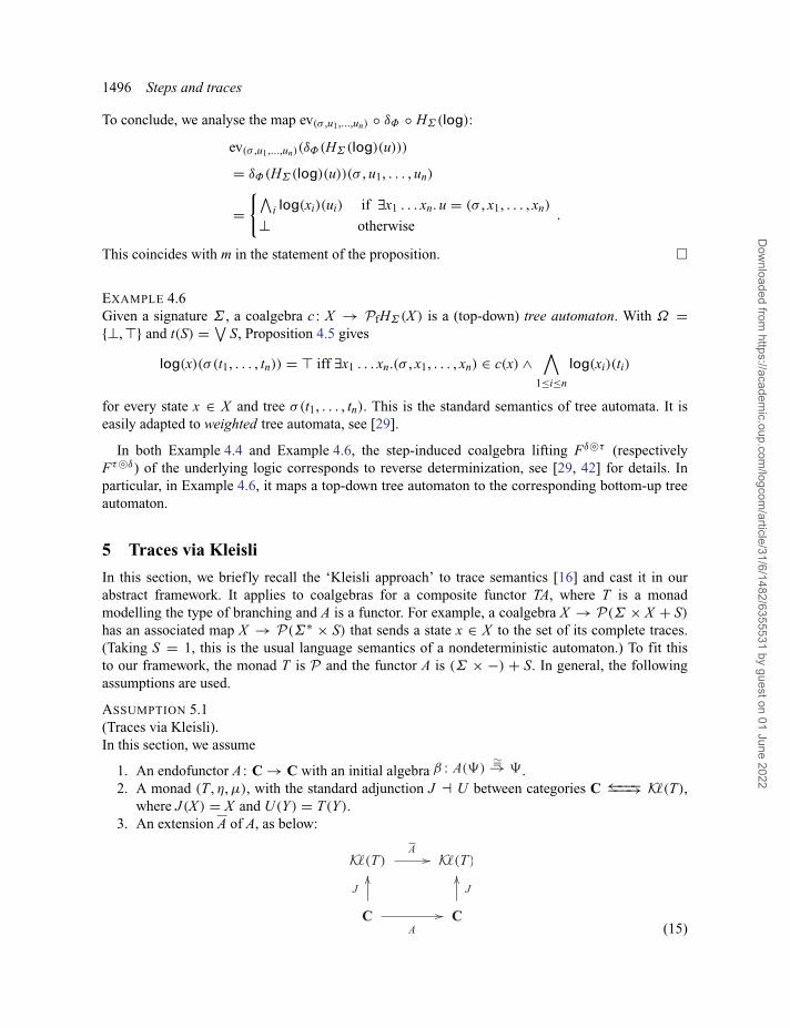
To conclude, we analyse the map ev(σ ,u1,...,un) ◦ δΦ ◦ HΣ(log):
ev(σ ,u1,...,un)(δΦ(HΣ(log)(u)))
= δΦ(HΣ(log)(u))(σ , u1, . . . , un)
={∧
i log(xi)(ui) if ∃x1 . . . xn. u = (σ , x1, . . . , xn)
⊥ otherwise.
This coincides with m in the statement of the proposition. �
EXAMPLE 4.6Given a signature Σ , a coalgebra c : X → PfHΣ(X ) is a (top-down) tree automaton. With Ω ={⊥, } and t(S) = ∨
S, Proposition 4.5 gives
log(x)(σ (t1, . . . , tn)) = iff ∃x1 . . . xn.(σ , x1, . . . , xn) ∈ c(x) ∧∧
1≤i≤n
log(xi)(ti)
for every state x ∈ X and tree σ(t1, . . . , tn). This is the standard semantics of tree automata. It iseasily adapted to weighted tree automata, see [29].
In both Example 4.4 and Example 4.6, the step-induced coalgebra lifting Fδ�τ (respectivelyFτ�δ) of the underlying logic corresponds to reverse determinization, see [29, 42] for details. Inparticular, in Example 4.6, it maps a top-down tree automaton to the corresponding bottom-up treeautomaton.
5 Traces via Kleisli
In this section, we brief ly recall the ‘Kleisli approach’ to trace semantics [16] and cast it in ourabstract framework. It applies to coalgebras for a composite functor TA, where T is a monadmodelling the type of branching and A is a functor. For example, a coalgebra X → P(Σ × X + S)
has an associated map X → P(Σ∗ × S) that sends a state x ∈ X to the set of its complete traces.(Taking S = 1, this is the usual language semantics of a nondeterministic automaton.) To fit thisto our framework, the monad T is P and the functor A is (Σ × −) + S. In general, the followingassumptions are used.
ASSUMPTION 5.1(Traces via Kleisli).In this section, we assume
1. An endofunctor A : C → C with an initial algebra .2. A monad (T , η, μ), with the standard adjunction J � U between categories C ←−−−−−−→ K�(T),
where J(X ) = X and U(Y ) = T(Y ).3. An extension A of A, as below:
(15)
Dow
nloaded from https://academ
ic.oup.com/logcom
/article/31/6/1482/6355531 by guest on 01 June 2022
Steps and traces 1497
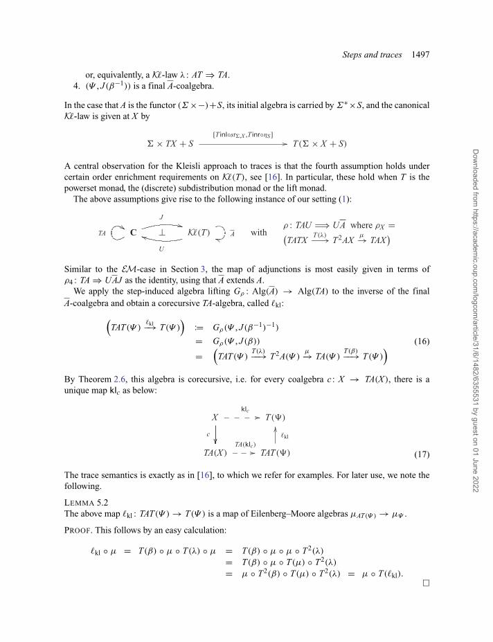
or, equivalently, a K�-law λ : AT ⇒ TA.4. (Ψ , J(β−1)) is a final A-coalgebra.
In the case that A is the functor (Σ ×−)+S, its initial algebra is carried by Σ∗×S, and the canonicalK�-law is given at X by
A central observation for the Kleisli approach to traces is that the fourth assumption holds undercertain order enrichment requirements on K�(T), see [16]. In particular, these hold when T is thepowerset monad, the (discrete) subdistribution monad or the lift monad.
The above assumptions give rise to the following instance of our setting (1):
Similar to the EM-case in Section 3, the map of adjunctions is most easily given in terms ofρ4 : TA ⇒ UAJ as the identity, using that A extends A.
We apply the step-induced algebra lifting Gρ : Alg(A) → Alg(TA) to the inverse of the finalA-coalgebra and obtain a corecursive TA-algebra, called �kl:(
TAT(Ψ )�kl−→ T(Ψ )
):= Gρ(Ψ , J(β−1)−1)
= Gρ(Ψ , J(β))
=(
TAT(Ψ )T(λ)−−→ T2A(Ψ )
μ−→ TA(Ψ )T(β)−−→ T(Ψ )
) (16)
By Theorem 2.6, this algebra is corecursive, i.e. for every coalgebra c : X → TA(X ), there is aunique map klc as below:
(17)
The trace semantics is exactly as in [16], to which we refer for examples. For later use, we note thefollowing.
LEMMA 5.2The above map �kl : TAT(Ψ ) → T(Ψ ) is a map of Eilenberg–Moore algebras μAT(Ψ ) → μΨ .
PROOF. This follows by an easy calculation:
�kl ◦ μ = T(β) ◦ μ ◦ T(λ) ◦ μ = T(β) ◦ μ ◦ μ ◦ T2(λ)
= T(β) ◦ μ ◦ T(μ) ◦ T2(λ)
= μ ◦ T2(β) ◦ T(μ) ◦ T2(λ) = μ ◦ T(�kl).�
Dow
nloaded from https://academ
ic.oup.com/logcom
/article/31/6/1482/6355531 by guest on 01 June 2022
1498 Steps and traces
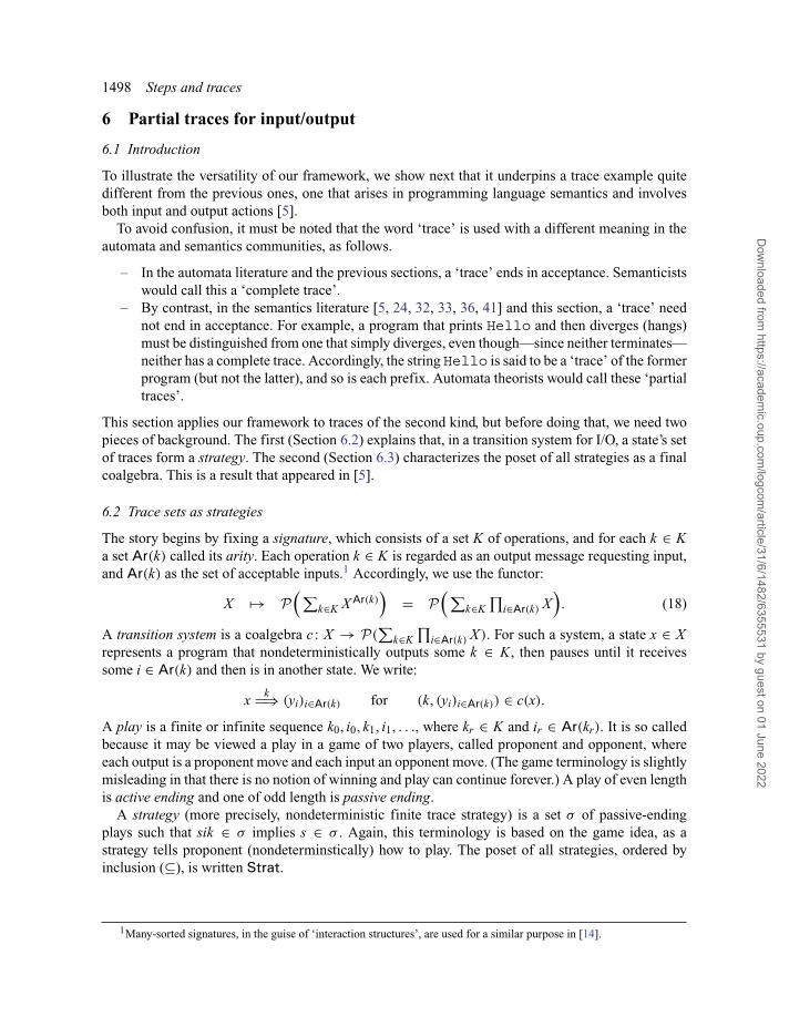
6 Partial traces for input/output
6.1 Introduction
To illustrate the versatility of our framework, we show next that it underpins a trace example quitedifferent from the previous ones, one that arises in programming language semantics and involvesboth input and output actions [5].
To avoid confusion, it must be noted that the word ‘trace’ is used with a different meaning in theautomata and semantics communities, as follows.
– In the automata literature and the previous sections, a ‘trace’ ends in acceptance. Semanticistswould call this a ‘complete trace’.
– By contrast, in the semantics literature [5, 24, 32, 33, 36, 41] and this section, a ‘trace’ neednot end in acceptance. For example, a program that prints Hello and then diverges (hangs)must be distinguished from one that simply diverges, even though—since neither terminates—neither has a complete trace. Accordingly, the string Hello is said to be a ‘trace’ of the formerprogram (but not the latter), and so is each prefix. Automata theorists would call these ‘partialtraces’.
This section applies our framework to traces of the second kind, but before doing that, we need twopieces of background. The first (Section 6.2) explains that, in a transition system for I/O, a state’s setof traces form a strategy. The second (Section 6.3) characterizes the poset of all strategies as a finalcoalgebra. This is a result that appeared in [5].
6.2 Trace sets as strategies
The story begins by fixing a signature, which consists of a set K of operations, and for each k ∈ Ka set Ar(k) called its arity. Each operation k ∈ K is regarded as an output message requesting input,and Ar(k) as the set of acceptable inputs.1 Accordingly, we use the functor:
X �→ P(∑
k∈K X Ar(k))
= P( ∑
k∈K∏
i∈Ar(k) X)
. (18)
A transition system is a coalgebra c : X → P(∑
k∈K∏
i∈Ar(k) X ). For such a system, a state x ∈ Xrepresents a program that nondeterministically outputs some k ∈ K, then pauses until it receivessome i ∈ Ar(k) and then is in another state. We write:
xk�⇒ (yi)i∈Ar(k) for (k, (yi)i∈Ar(k)) ∈ c(x).
A play is a finite or infinite sequence k0, i0, k1, i1, . . ., where kr ∈ K and ir ∈ Ar(kr). It is so calledbecause it may be viewed a play in a game of two players, called proponent and opponent, whereeach output is a proponent move and each input an opponent move. (The game terminology is slightlymisleading in that there is no notion of winning and play can continue forever.) A play of even lengthis active ending and one of odd length is passive ending.
A strategy (more precisely, nondeterministic finite trace strategy) is a set σ of passive-endingplays such that sik ∈ σ implies s ∈ σ . Again, this terminology is based on the game idea, as astrategy tells proponent (nondeterminstically) how to play. The poset of all strategies, ordered byinclusion (⊆), is written Strat.
1Many-sorted signatures, in the guise of ‘interaction structures’, are used for a similar purpose in [14].
Dow
nloaded from https://academ
ic.oup.com/logcom
/article/31/6/1482/6355531 by guest on 01 June 2022
Steps and traces 1499
Let (X , c) be a transition system and x ∈ X a state. A passive-ending play k0, i0, . . . , kn is said tobe a trace of x when there is a sequence
x = x0k0�⇒ (y0
i )i∈Ar(k0) , y0i0 = x1
k1�⇒ (y1i )i∈Ar(k1) , · · ·
The set of all such traces forms a strategy. Note that active-ending traces need not be considered,since these are determined by the passive-ending traces. Infinite traces are not considered in [5], norare they here. Conversely, every strategy can be obtained in this way [5, Proposition 6.1].
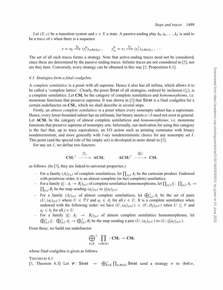
6.3 Strategies form a final coalgebra
A complete semilattice is a poset with all suprema. Hence it also has all infima, which allows it tobe called a ‘complete lattice’. Clearly, the poset Strat of all strategies, ordered by inclusion (⊆), isa complete semilattice. Let CSL be the category of complete semilattices and homomorphisms, i.e.monotone functions that preserve suprema. It was shown in [5] that Strat is a final coalgebra for acertain endofunctor on CSL, which we shall describe in several steps.
Firstly, an almost complete semilattice is a poset where every nonempty subset has a supremum.Hence, every lower-bounded subset has an infimum, but binary meets a∧b need not exist in general.Let ACSL be the category of almost complete semilattices and homomorphisms, i.e. monotonefunctions that preserve suprema of nonempty sets. Informally, our motivation for using this categoryis the fact that, up to trace equivalence, an I/O action such as printing commutes with binarynondeterminism, and more generally with I-ary nondeterministic choice for any nonempty set I .This point (and the special role of the empty set) is developed in more detail in [5].
For any set J , we define two functors:
as follows. (In [5], they are linked to universal properties.)
– For a family (Aj)j∈J of complete semilattices, let∏
j∈J Aj be the cartesian product. Endowedwith pointwise order, it is an almost complete (in fact complete) semilattice.
– For a family (fj : Aj → Bj)j∈J of complete semilattice homomorphisms, let∏
j∈J fj :∏
j∈J Aj →∏j∈J Bj be the map sending (aj)j∈J to (fjaj)j∈J .
– For a family (Aj)j∈J of almost complete semilattices, let⊕⊥
j∈J Aj be the set of pairs(U , (aj)j∈U ) where U ∈ PJ and aj ∈ Aj for all j ∈ U . It is a complete semilattice whenendowed with the following order: we have (U , (aj)j∈U ) � (V , (bj)j∈V ) when U ⊆ V andaj � bj for all j ∈ U .
– For a family (fj : Aj → Bj)j∈J of almost complete semilattice homomorphisms, let⊕⊥j∈J fj :
⊕⊥j∈J Aj → ⊕⊥
j∈J Bj be the map sending a pair (U , (aj)j∈U ) to (U , (fjaj)j∈U ).
From these, we build our endofunctor⊕k∈K
⊥ ∏i∈Ar(k)
: CSL → CSL
whose final coalgebra is given as follows.
THEOREM 6.1[5, Theorem 6.3] Let Ψ : Strat → ⊕⊥
k∈K∏
i∈Ar(k) Strat send a strategy σ to (Init σ ,
Dow
nloaded from https://academ
ic.oup.com/logcom
/article/31/6/1482/6355531 by guest on 01 June 2022
1500 Steps and traces
((σ/kii)i∈Ar(k))k∈Init σ ), where
Init σdef= {k ∈ K | (k) ∈ σ }
σ/kidef= {s | k.i.s ∈ σ }
Then (Strat, Ψ ) is a final⊕⊥
k∈K∏
i∈Ar(k)-coalgebra.
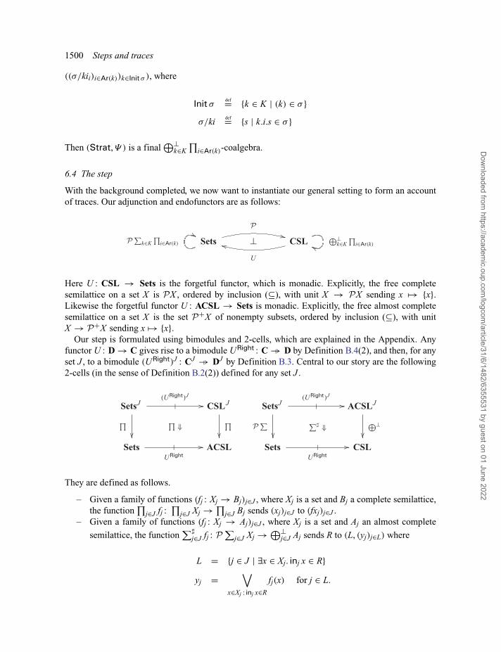
6.4 The step
With the background completed, we now want to instantiate our general setting to form an accountof traces. Our adjunction and endofunctors are as follows:
Here U : CSL → Sets is the forgetful functor, which is monadic. Explicitly, the free completesemilattice on a set X is PX , ordered by inclusion (⊆), with unit X → PX sending x �→ {x}.Likewise the forgetful functor U : ACSL → Sets is monadic. Explicitly, the free almost completesemilattice on a set X is the set P+X of nonempty subsets, ordered by inclusion (⊆), with unitX → P+X sending x �→ {x}.
Our step is formulated using bimodules and 2-cells, which are explained in the Appendix. Anyfunctor U : D → C gives rise to a bimodule URight : C →� D by Definition B.4(2), and then, for anyset J , to a bimodule (URight)J : CJ →� DJ by Definition B.3. Central to our story are the following2-cells (in the sense of Definition B.2(2)) defined for any set J .
They are defined as follows.
– Given a family of functions (fj : Xj → Bj)j∈J , where Xj is a set and Bj a complete semilattice,the function
∏j∈J fj :
∏j∈J Xj → ∏
j∈J Bj sends (xj)j∈J to (fxj)j∈J .– Given a family of functions (fj : Xj → Aj)j∈J , where Xj is a set and Aj an almost complete
semilattice, the function∑�
j∈J fj : P∑
j∈J Xj → ⊕⊥j∈J Aj sends R to (L, (yj)j∈L) where
L = {j ∈ J | ∃x ∈ Xj. inj x ∈ R}yj =
∨x∈Xj : inj x∈R
fj(x) for j ∈ L.
Dow
nloaded from https://academ
ic.oup.com/logcom
/article/31/6/1482/6355531 by guest on 01 June 2022
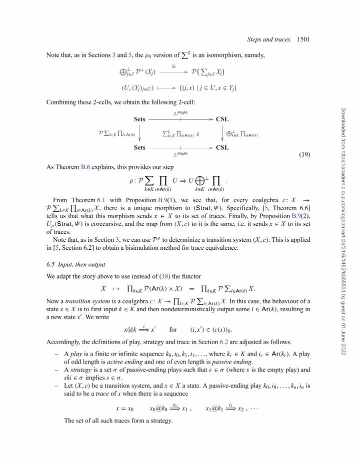
Steps and traces 1501
Note that, as in Sections 3 and 5, the ρ4 version of∑� is an isomorphism, namely,
Combining these 2-cells, we obtain the following 2-cell:
(19)
As Theorem B.6 explains, this provides our step
ρ : P∑k∈K
∏i∈Ar(k)
U ⇒ U⊕k∈K
⊥ ∏i∈Ar(k)
.
From Theorem 6.1 with Proposition B.9(1), we see that, for every coalgebra c : X →P
∑k∈K
∏i∈Ar(k) X , there is a unique morphism to (Strat, Ψ ). Specifically, [5, Theorem 6.6]
tells us that what this morphism sends x ∈ X to its set of traces. Finally, by Proposition B.9(2),Uρ(Strat, Ψ ) is corecursive, and the map from (X , c) to it is the same, i.e. it sends x ∈ X to its setof traces.
Note that, as in Section 3, we can use Pρ to determinize a transition system (X , c). This is appliedin [5, Section 6.2] to obtain a bisimulation method for trace equivalence.
6.5 Input, then output
We adapt the story above to use instead of (18) the functor
X �→ ∏k∈K P(Ar(k) × X ) = ∏
k∈K P∑
i∈Ar(k) X .
Now a transition system is a coalgebra c : X → ∏k∈K P
∑i∈Ar(k) X . In this case, the behaviour of a
state x ∈ X is to first input k ∈ K and then nondeterministically output some i ∈ Ar(k), resulting ina new state x′. We write
x@ki�⇒ x′ for (i, x′) ∈ (c(x))k .
Accordingly, the definitions of play, strategy and trace in Section 6.2 are adjusted as follows.
– A play is a finite or infinite sequence k0, i0, k1, i1, . . ., where kr ∈ K and ir ∈ Ar(kr). A playof odd length is active ending and one of even length is passive ending.
– A strategy is a set σ of passive-ending plays such that ε ∈ σ (where ε is the empty play) andski ∈ σ implies s ∈ σ .
– Let (X , c) be a transition system, and x ∈ X a state. A passive-ending play k0, i0, . . . , kn, in issaid to be a trace of x when there is a sequence
x = x0 x0@k0i0�⇒ x1 , x1@k1
i1�⇒ x2 , · · ·The set of all such traces form a strategy.
Dow
nloaded from https://academ
ic.oup.com/logcom
/article/31/6/1482/6355531 by guest on 01 June 2022
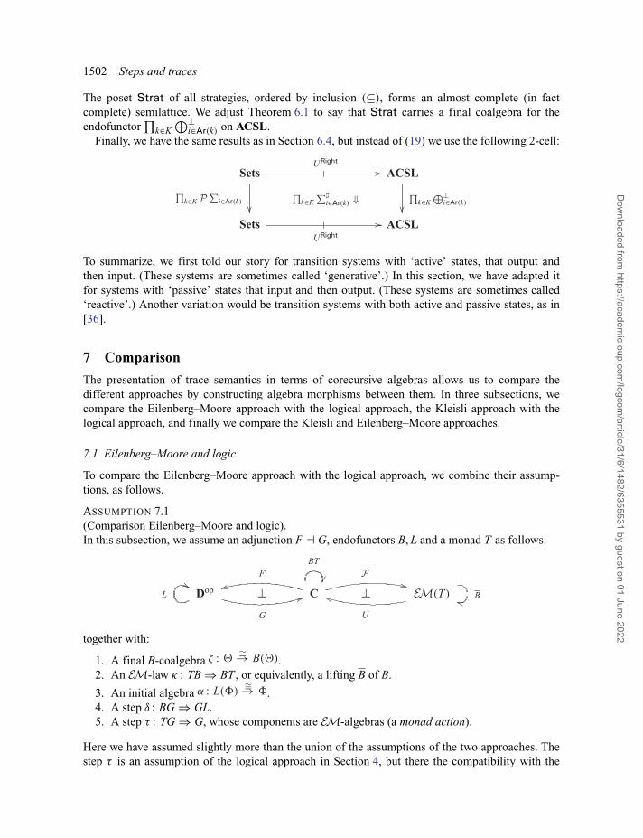
1502 Steps and traces
The poset Strat of all strategies, ordered by inclusion (⊆), forms an almost complete (in factcomplete) semilattice. We adjust Theorem 6.1 to say that Strat carries a final coalgebra for theendofunctor
∏k∈K
⊕⊥i∈Ar(k) on ACSL.
Finally, we have the same results as in Section 6.4, but instead of (19) we use the following 2-cell:
To summarize, we first told our story for transition systems with ‘active’ states, that output andthen input. (These systems are sometimes called ‘generative’.) In this section, we have adapted itfor systems with ‘passive’ states that input and then output. (These systems are sometimes called‘reactive’.) Another variation would be transition systems with both active and passive states, as in[36].
7 Comparison
The presentation of trace semantics in terms of corecursive algebras allows us to compare thedifferent approaches by constructing algebra morphisms between them. In three subsections, wecompare the Eilenberg–Moore approach with the logical approach, the Kleisli approach with thelogical approach, and finally we compare the Kleisli and Eilenberg–Moore approaches.
7.1 Eilenberg–Moore and logic
To compare the Eilenberg–Moore approach with the logical approach, we combine their assump-tions, as follows.
ASSUMPTION 7.1(Comparison Eilenberg–Moore and logic).In this subsection, we assume an adjunction F � G, endofunctors B, L and a monad T as follows:
together with:
1. A final B-coalgebra .2. An EM-law κ : TB ⇒ BT , or equivalently, a lifting B of B.
3. An initial algebra .4. A step δ : BG ⇒ GL.5. A step τ : TG ⇒ G, whose components are EM-algebras (a monad action).
Here we have assumed slightly more than the union of the assumptions of the two approaches. Thestep τ is an assumption of the logical approach in Section 4, but there the compatibility with the
Dow
nloaded from https://academ
ic.oup.com/logcom
/article/31/6/1482/6355531 by guest on 01 June 2022
Steps and traces 1503
monad structure was not assumed—simply because T was not assumed to be a monad before. Here,we use this assumption as a first compatibility requirement between the logical and Eilenberg–Mooreapproaches.
We note that τ being a monad action is the same thing as τ being an EM-law, involving themonad T on the left and the identity monad on the right. The next result is therefore an instance ofTheorem 2.3.
LEMMA 7.2The following are equivalent:
1. a monad action τ1 : TG ⇒ G;2. a map τ2 : F ⇒ FT , satisfying the obvious dual action equations;3. a monad morphism τ4 : T ⇒ GF;4. an extension F : K�(T) → Dop (= K�(Id)) of F.5. a lifting G : Dop → EM(T) of G.
Such monad actions and the corresponding liftings are used, e.g. in [15, 17, 20] where F is calledPred. We use · to indicate liftings associated with the step τ , in order to create a distinction with thelifting · associated with κ .
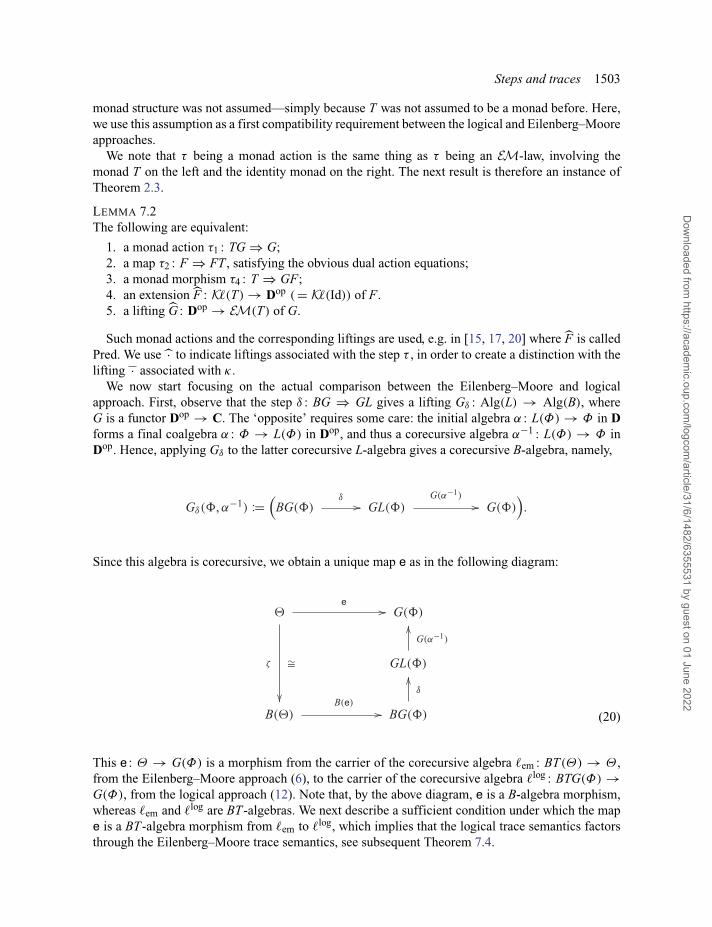
We now start focusing on the actual comparison between the Eilenberg–Moore and logicalapproach. First, observe that the step δ : BG ⇒ GL gives a lifting Gδ : Alg(L) → Alg(B), whereG is a functor Dop → C. The ‘opposite’ requires some care: the initial algebra α : L(Φ) → Φ in Dforms a final coalgebra α : Φ → L(Φ) in Dop, and thus a corecursive algebra α−1 : L(Φ) → Φ inDop. Hence, applying Gδ to the latter corecursive L-algebra gives a corecursive B-algebra, namely,
Since this algebra is corecursive, we obtain a unique map e as in the following diagram:
(20)
This e : Θ → G(Φ) is a morphism from the carrier of the corecursive algebra �em : BT(Θ) → Θ ,from the Eilenberg–Moore approach (6), to the carrier of the corecursive algebra �log : BTG(Φ) →G(Φ), from the logical approach (12). Note that, by the above diagram, e is a B-algebra morphism,whereas �em and �log are BT-algebras. We next describe a sufficient condition under which the mape is a BT-algebra morphism from �em to �log, which implies that the logical trace semantics factorsthrough the Eilenberg–Moore trace semantics, see subsequent Theorem 7.4.
Dow
nloaded from https://academ
ic.oup.com/logcom
/article/31/6/1482/6355531 by guest on 01 June 2022
1504 Steps and traces
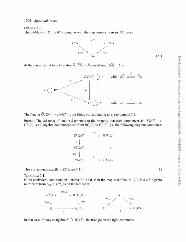
LEMMA 7.3The EM-law κ : TB ⇒ BT commutes with the step compositions in (11), as in
(21)
iff there is a natural transformation δ : BG ⇒ GL satisfying U (δ) = δ in
The functor G : Dop → EM(T) is the lifting corresponding to τ , see Lemma 7.2.
PROOF. The existence of such a δ amounts to the property that each component δX : BG(X ) →GL(X ) is a T-algebra homomorphism from BG(X ) to GL(X ), i.e. the following diagram commutes:
This corresponds exactly to (21), see (11). �THEOREM 7.4If the equivalent conditions in Lemma 7.3 hold, then the map e defined in (20) is a BT-algebramorphism from �em to �log, as on the left below.
In that case, for any coalgebra Xc→ BT(X ), the triangle on the right commutes.
Dow
nloaded from https://academ
ic.oup.com/logcom
/article/31/6/1482/6355531 by guest on 01 June 2022
Steps and traces 1505
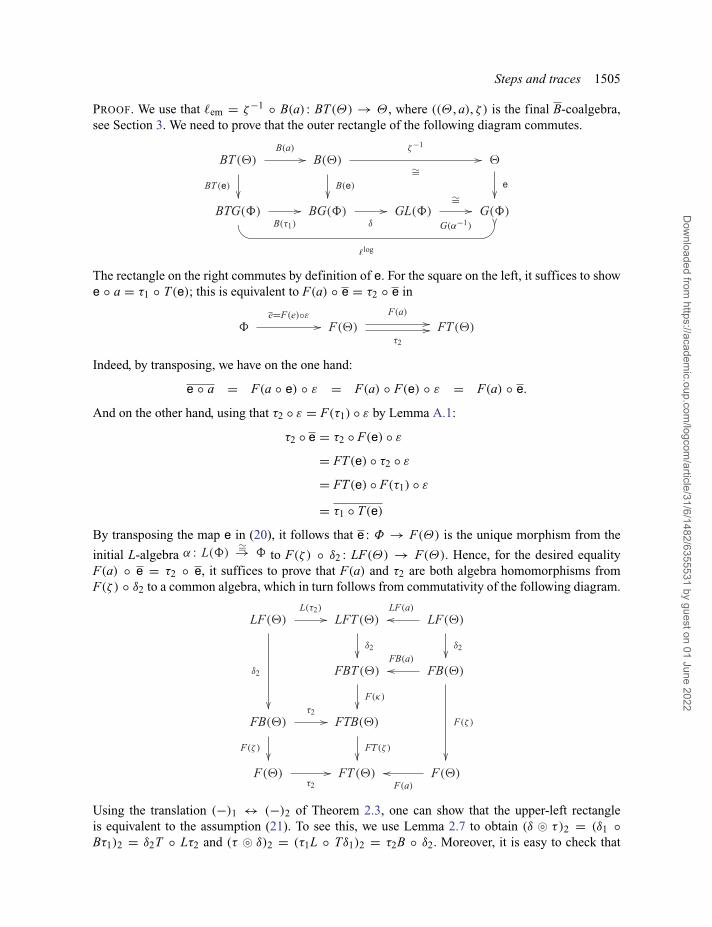
PROOF. We use that �em = ζ−1 ◦ B(a) : BT(Θ) → Θ , where ((Θ , a), ζ ) is the final B-coalgebra,see Section 3. We need to prove that the outer rectangle of the following diagram commutes.
The rectangle on the right commutes by definition of e. For the square on the left, it suffices to showe ◦ a = τ1 ◦ T(e); this is equivalent to F(a) ◦ e = τ2 ◦ e in
Indeed, by transposing, we have on the one hand:
e ◦ a = F(a ◦ e) ◦ ε = F(a) ◦ F(e) ◦ ε = F(a) ◦ e.
And on the other hand, using that τ2 ◦ ε = F(τ1) ◦ ε by Lemma A.1:
τ2 ◦ e = τ2 ◦ F(e) ◦ ε
= FT(e) ◦ τ2 ◦ ε
= FT(e) ◦ F(τ1) ◦ ε
= τ1 ◦ T(e)
By transposing the map e in (20), it follows that e : Φ → F(Θ) is the unique morphism from the
initial L-algebra to F(ζ ) ◦ δ2 : LF(Θ) → F(Θ). Hence, for the desired equalityF(a) ◦ e = τ2 ◦ e, it suffices to prove that F(a) and τ2 are both algebra homomorphisms fromF(ζ ) ◦ δ2 to a common algebra, which in turn follows from commutativity of the following diagram.
Using the translation (−)1 ↔ (−)2 of Theorem 2.3, one can show that the upper-left rectangleis equivalent to the assumption (21). To see this, we use Lemma 2.7 to obtain (δ � τ)2 = (δ1 ◦Bτ1)2 = δ2T ◦ Lτ2 and (τ � δ)2 = (τ1L ◦ Tδ1)2 = τ2B ◦ δ2. Moreover, it is easy to check that
Dow
nloaded from https://academ
ic.oup.com/logcom
/article/31/6/1482/6355531 by guest on 01 June 2022
1506 Steps and traces
(δ1 ◦ Bτ1 ◦ κG)2 = Fκ ◦ (δ1 ◦ Bτ1)2. The lower-right rectangle commutes since ((Θ , a), ζ ) is aB-coalgebra. The other two squares commute by naturality.
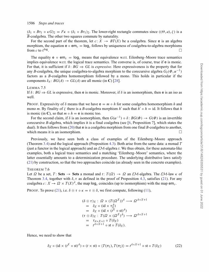
For the second part of the theorem, let c : X → BT(X ) be a coalgebra. Since e is an algebramorphism, the equation e ◦ emc = logc follows by uniqueness of coalgebra-to-algebra morphismsfrom c to �log. �
The equality e ◦ emc = logc means that equivalence w.r.t. Eilenberg–Moore trace semanticsimplies equivalence w.r.t. the logical trace semantics. The converse is, of course, true if e is monic.For that, it is sufficient if δ : BG ⇒ GL is expressive. Here expressiveness is the property that forany B-coalgebra, the unique coalgebra-to-algebra morphism to the corecursive algebra Gδ(Φ, α−1)
factors as a B-coalgebra homomorphism followed by a mono. This holds in particular if thecomponents δA : BG(A) → GL(A) are all monic (in C) [28].
LEMMA 7.5If δ : BG ⇒ GL is expressive, then e is monic. Moreover, if δ is an isomorphism, then e is an iso aswell.
PROOF. Expressivity of δ means that we have e = m ◦ h for some coalgebra homomorphism h andmono m. By finality of ζ there is a B-coalgebra morphism h′ such that h′ ◦ h = id. It follows that his monic (in C), so that m ◦ h = e is monic too.
For the second claim, if δ is an isomorphism, then G(α−1) ◦ δ : BG(Φ) → G(Φ) is an invertiblecorecursive B-algebra, which implies it is a final coalgebra (see [6, Proposition 7], which states thedual). It then follows from (20) that e is a coalgebra morphism from one final B-coalgebra to another,which means it is an isomorphism. �
Previously, we have seen both a class of examples of the Eilenberg–Moore approach(Theorem 3.4) and the logical approach (Proposition 4.3). Both arise from the same data: a monad T(just a functor in the logical approach) and an EM-algebra t. We thus obtain, for these automata-likeexamples, both a logical trace semantics and a matching ‘Eilenberg–Moore’ semantics, where thelatter essentially amounts to a determinization procedure. The underlying distributive laws satisfy(21) by construction, so that the two approaches coincide (as already seen in the concrete examples).
THEOREM 7.6Let Ω be a set, T : Sets → Sets a monad and t : T(Ω) → Ω an EM-algebra. The EM-law κ ofTheorem 3.4, together with δ, τ as defined in the proof of Proposition 4.3, satisfies (21). For anycoalgebra c : X → Ω × T(X )A, the map logc coincides (up to isomorphism) with the map emc.
PROOF. To prove (21), i.e. δ � τ ◦ κ = τ � δ, we first compute, following (11),
(δ � τ)X : Ω × (T(ΩX ))A −→ ΩA×X+1
= δX ◦ (id × τAX )
= δX ◦ (id × (tX ◦ st)A)
(τ � δ)X : T(Ω × (ΩX )A) −→ ΩA×X+1
= τA×X+1 ◦ T(δX )
= tA×X+1 ◦ st ◦ T(δX ).
Hence, we need to show that
δX ◦ (id × (tX ◦ st)A) ◦ (t × st) ◦ 〈T(π1), T(π2)〉 = tA×X+1 ◦ st ◦ T(δX ) (22)
Dow
nloaded from https://academ
ic.oup.com/logcom
/article/31/6/1482/6355531 by guest on 01 June 2022
Steps and traces 1507
for every set X . To this end, let S ∈ T(Ω × (ΩX )A) and u ∈ (A × X + 1). We first spell out theright-hand side:
(tA×X+1 ◦ st ◦ T(δX )(S))(u)
= t((st ◦ T(δX )(S))(u))
= t(T(evu ◦ δX )(S))
={
t(T(π1)(S)) if u = ∗ ∈ 1
t(T(evx ◦ eva ◦ π2)(S)) if u = (a, x) ∈ A × X
In the last step, we used the definition of δ:
ev∗ ◦ δX (ω, f ) = δX (ω, f )(∗) = ω = π1(ω, f ) ,
ev(a,x) ◦ δX (ω, f ) = δX (ω, f )(a, x) = f (a)(x) = evx ◦ eva ◦ π2(ω, f ) .
For the left-hand side of (22), distinguish cases ∗ ∈ 1 and (a, x) ∈ A × X .
(δX ◦ (id × (tX ◦ st)A) ◦ (t × st) ◦ 〈T(π1), T(π2)〉(S))(∗)
= π1(id × (tX ◦ st)A) ◦ (t × st) ◦ 〈T(π1), T(π2)〉(S))
= t(T(π1)(S))
which matches the right-hand side of (22). For (a, x) ∈ A × X , we have
(δX ◦ (id × (tX ◦ st)A) ◦ (t × st) ◦ 〈T(π1), T(π2)〉(S))(a, x)
= (((tX ◦ st)A ◦ st)(T(π2)(S)))(a)(x)
= (((tX )A ◦ stA ◦ st)(T(π2)(S)))(a)(x)
= (tX ◦ st(st(T(π2)(S))(a)))(x)
= (tX ◦ st(T(eva)(T(π2)(S)))(x)
= (tX ◦ st(T(eva ◦ π2)(S)))(x)
= t(st(T(eva ◦ π2)(S))(x))
= t(T(evx) ◦ T(eva ◦ π2)(S))
= t(T(evx ◦ eva ◦ π2)(S))
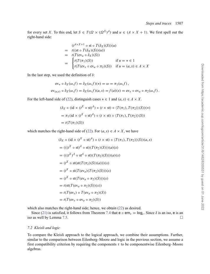
which also matches the right-hand side; hence, we obtain (22) as desired.Since (21) is satisfied, it follows from Theorem 7.4 that e ◦ emc = logc. Since δ is an iso, e is an
iso as well by Lemma 7.5. �
7.2 Kleisli and logic
To compare the Kleisli approach to the logical approach, we combine their assumptions. Further,similar to the comparison between Eilenberg–Moore and logic in the previous section, we assume afirst compatibility criterion by requiring the components τ to be componentwise Eilenberg–Moorealgebras.
Dow
nloaded from https://academ
ic.oup.com/logcom
/article/31/6/1482/6355531 by guest on 01 June 2022
1508 Steps and traces
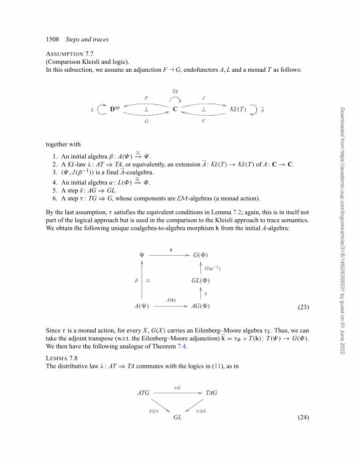
ASSUMPTION 7.7(Comparison Kleisli and logic).In this subsection, we assume an adjunction F � G, endofunctors A, L and a monad T as follows:
together with
1. An initial algebra β : A(Ψ )∼=−→ Ψ .
2. A K�-law λ : AT ⇒ TA, or equivalently, an extension A : K�(T) → K�(T) of A : C → C.3. (Ψ , J(β−1)) is a final A-coalgebra.
4. An initial algebra α : L(Φ)∼=−→ Φ.
5. A step δ : AG ⇒ GL.6. A step τ : TG ⇒ G, whose components are EM-algebras (a monad action).
By the last assumption, τ satisfies the equivalent conditions in Lemma 7.2; again, this is in itself notpart of the logical approach but is used in the comparison to the Kleisli approach to trace semantics.We obtain the following unique coalgebra-to-algebra morphism k from the initial A-algebra:
(23)
Since τ is a monad action, for every X , G(X ) carries an Eilenberg–Moore algebra τX . Thus, we cantake the adjoint transpose (w.r.t. the Eilenberg–Moore adjunction) k = τΦ ◦ T(k) : T(Ψ ) → G(Φ).We then have the following analogue of Theorem 7.4.
LEMMA 7.8The distributive law λ : AT ⇒ TA commutes with the logics in (11), as in
(24)
Dow
nloaded from https://academ
ic.oup.com/logcom
/article/31/6/1482/6355531 by guest on 01 June 2022
Steps and traces 1509
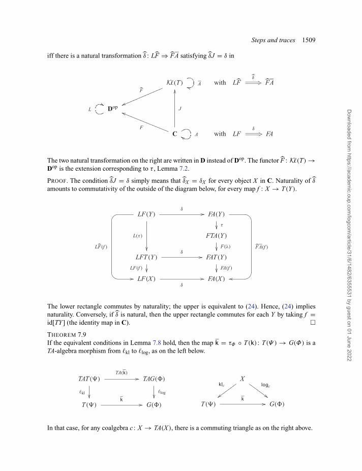
iff there is a natural transformation δ : LF ⇒ FA satisfying δJ = δ in
The two natural transformation on the right are written in D instead of Dop. The functor F : K�(T) →Dop is the extension corresponding to τ , Lemma 7.2.
PROOF. The condition δJ = δ simply means that δX = δX for every object X in C. Naturality of δ
amounts to commutativity of the outside of the diagram below, for every map f : X → T(Y ).
The lower rectangle commutes by naturality; the upper is equivalent to (24). Hence, (24) impliesnaturality. Conversely, if δ is natural, then the upper rectangle commutes for each Y by taking f =id[TY ] (the identity map in C). �THEOREM 7.9If the equivalent conditions in Lemma 7.8 hold, then the map k = τΦ ◦ T(k) : T(Ψ ) → G(Φ) is aTA-algebra morphism from �kl to �log, as on the left below.
In that case, for any coalgebra c : X → TA(X ), there is a commuting triangle as on the right above.
Dow
nloaded from https://academ
ic.oup.com/logcom
/article/31/6/1482/6355531 by guest on 01 June 2022
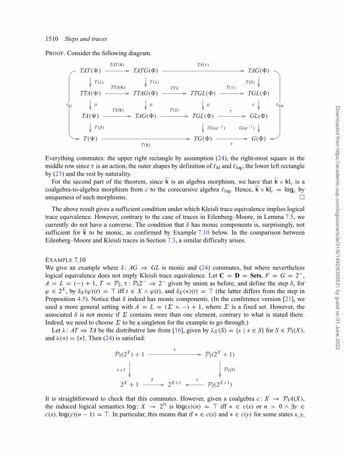
1510 Steps and traces
PROOF. Consider the following diagram.
Everything commutes: the upper right rectangle by assumption (24), the right-most square in themiddle row since τ is an action, the outer shapes by definition of �kl and �log, the lower left rectangleby (23) and the rest by naturality.
For the second part of the theorem, since k is an algebra morphism, we have that k ◦ klc is acoalgebra-to-algebra morphism from c to the corecursive algebra �log. Hence, k ◦ klc = logc byuniqueness of such morphisms. �
The above result gives a sufficient condition under which Kleisli trace equivalence implies logicaltrace equivalence. However, contrary to the case of traces in Eilenberg–Moore, in Lemma 7.5, wecurrently do not have a converse. The condition that δ has monic components is, surprisingly, notsufficient for k to be monic, as confirmed by Example 7.10 below. In the comparison betweenEilenberg–Moore and Kleisli traces in Section 7.3, a similar difficulty arises.
EXAMPLE 7.10We give an example where δ : AG ⇒ GL is monic and (24) commutes, but where neverthelesslogical equivalence does not imply Kleisli trace equivalence. Let C = D = Sets, F = G = 2−,A = L = (−) + 1, T = Pf, τ : Pf2− ⇒ 2− given by union as before, and define the step δ, forϕ ∈ 2X , by δX (ϕ)(t) = iff t ∈ X ∧ ϕ(t), and δX (∗)(t) = (the latter differs from the step inProposition 4.5). Notice that δ indeed has monic components. (In the conference version [21], weused a more general setting with A = L = (Σ × −) + 1, where Σ is a fixed set. However, theassociated δ is not monic if Σ contains more than one element, contrary to what is stated there.Indeed, we need to choose Σ to be a singleton for the example to go through.)
Let λ : AT ⇒ TA be the distributive law from [16], given by λX (S) = {x | x ∈ S} for S ∈ Pf(X ),and λ(∗) = {∗}. Then (24) is satisfied:
It is straightforward to check that this commutes. However, given a coalgebra c : X → PfA(X ),the induced logical semantics log : X → 2N is log(x)(n) = iff ∗ ∈ c(x) or n > 0 ∧ ∃y ∈c(x). log(y)(n − 1) = . In particular, this means that if ∗ ∈ c(x) and ∗ ∈ c(y) for some states x, y,
Dow
nloaded from https://academ
ic.oup.com/logcom
/article/31/6/1482/6355531 by guest on 01 June 2022

Steps and traces 1511
then they are trace equivalent. This differs from the Kleisli semantics, which amounts to the usuallanguage semantics of non-deterministic automata (over a singleton alphabet) [16].
Cîrstea [9] compares logical traces to a ‘path-based semantics’, which resembles the Kleisliapproach (as well as [31]) but does not require a final A-coalgebra. In particular, given a commutativemonad T on Sets and a signature Σ , she considers a canonical distributive law λ : HΣT ⇒ THΣ ,which coincides with the one in [16]. Cîrstea shows that, with Ω = T(1), t = μ1 : TT(1) → T(1)
and δ from the proof of Proposition 4.5 (assuming T1 to have enough structure to define that logic),the triangle (24) commutes (see [9, Lemma 5.12]).
7.3 Kleisli and Eilenberg–Moore
To compare the Eilenberg–Moore and Kleisli approaches, we first combine their assumptions. TheKleisli approach applies to TA-coalgebras; to match this, we make use of the variant of the Eilenberg–Moore approach for TA-coalgebras presented in Section 3.1. The latter approach uses a lifting of afunctor B as well as a step relating A and B.
ASSUMPTION 7.11(Comparison Kleisli and Eilenberg–Moore).In this subsection, we assume to endofunctors A, B and a monad T , on a base category C, and liftingsA, B to Kleisli and Eilenberg–Moore-categories as follows:
In this situation, we further assume the following ingredients, which combine earlier assumptions.
1. An initial algebra β : A(Ψ )∼=−→ Ψ .
2. A K�-law λ : AT ⇒ TA, or equivalently, an extension A : K�(T) → K�(T) of the functor A.3. (Ψ , J(β−1)) is a final A-coalgebra.4. An EM-law κ : TB ⇒ BT , or equivalently, a lifting B : EM(T) → EM(T).
5. A final coalgebra ζ : Θ∼=−→ B(Θ).
6. A step ρ : AU ⇒ UB.
The step ρ : AU ⇒ UB is an assumption of the Eilenberg–Moore approach for TA-coalgebras inSection 3.1, defined on top of the assumptions for the Eilenberg–Moore approach for BT-coalgebras.Under a further assumption such a law corresponds to an extension natural transformation as in [22],see Proposition 7.12.
Recall from Section 3 that the final B-coalgebra (Θ , ζ ) gives rise to a final B-coalgebra((Θ , a), ζ ). We will make use of the counit ε of the EM-adjunction F � U as a step Uε : TU ⇒ U .Its components are EM-algebras. For the trace semantics of TA-coalgebras via Eilenberg–Moore,see Section 3.1, we make use of the composed step:
(25)
These assumptions form an instance of the assumptions in Section 7.2, where we compared Kleislito logical trace semantics. In particular, in the latter we instantiate Dop with EM(T), L with B, δ with
Dow
nloaded from https://academ
ic.oup.com/logcom
/article/31/6/1482/6355531 by guest on 01 June 2022
1512 Steps and traces
ρ : AU ⇒ UB and τ with Uε : UT ⇒ U . Thus, we immediately obtain the comparison result fromTheorem 7.9. For presentation purposes, we restate the relevant results and definitions.
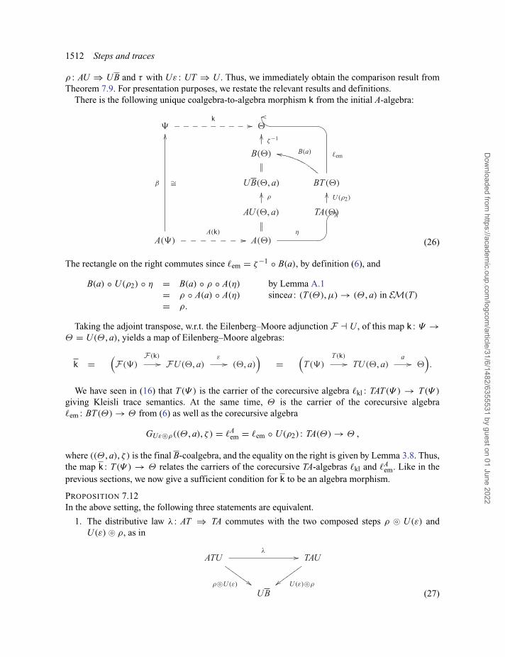
There is the following unique coalgebra-to-algebra morphism k from the initial A-algebra:
(26)
The rectangle on the right commutes since �em = ζ−1 ◦ B(a), by definition (6), and
B(a) ◦ U(ρ2) ◦ η = B(a) ◦ ρ ◦ A(η) by Lemma A.1= ρ ◦ A(a) ◦ A(η) sincea : (T(Θ), μ) → (Θ , a) in EM(T)
= ρ.
Taking the adjoint transpose, w.r.t. the Eilenberg–Moore adjunction F � U , of this map k : Ψ →Θ = U(Θ , a), yields a map of Eilenberg–Moore algebras:
We have seen in (16) that T(Ψ ) is the carrier of the corecursive algebra �kl : TAT(Ψ ) → T(Ψ )
giving Kleisli trace semantics. At the same time, Θ is the carrier of the corecursive algebra�em : BT(Θ) → Θ from (6) as well as the corecursive algebra
GUε�ρ((Θ , a), ζ ) = �Aem = �em ◦ U(ρ2) : TA(Θ) → Θ ,
where ((Θ , a), ζ ) is the final B-coalgebra, and the equality on the right is given by Lemma 3.8. Thus,the map k : T(Ψ ) → Θ relates the carriers of the corecursive TA-algebras �kl and �A
em. Like in theprevious sections, we now give a sufficient condition for k to be an algebra morphism.
PROPOSITION 7.12In the above setting, the following three statements are equivalent.
1. The distributive law λ : AT ⇒ TA commutes with the two composed steps ρ � U(ε) andU(ε) � ρ, as in
(27)
Dow
nloaded from https://academ
ic.oup.com/logcom
/article/31/6/1482/6355531 by guest on 01 June 2022
Steps and traces 1513
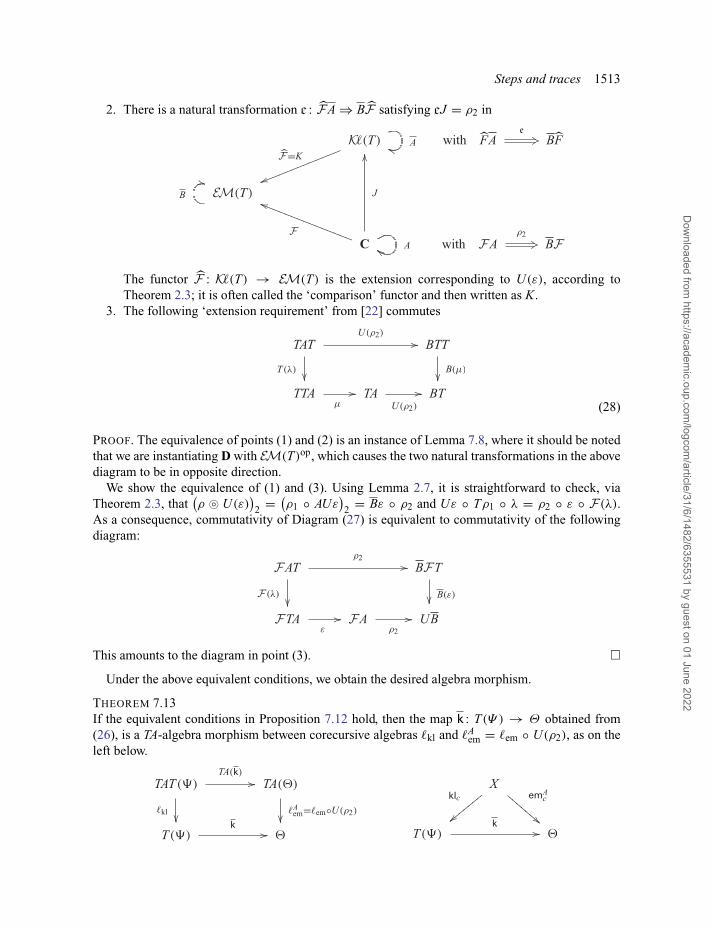
2. There is a natural transformation e : FA ⇒ BF satisfying eJ = ρ2 in
The functor F : K�(T) → EM(T) is the extension corresponding to U(ε), according toTheorem 2.3; it is often called the ‘comparison’ functor and then written as K.
3. The following ‘extension requirement’ from [22] commutes
(28)
PROOF. The equivalence of points (1) and (2) is an instance of Lemma 7.8, where it should be notedthat we are instantiating D with EM(T)op, which causes the two natural transformations in the abovediagram to be in opposite direction.
We show the equivalence of (1) and (3). Using Lemma 2.7, it is straightforward to check, viaTheorem 2.3, that
(ρ � U(ε)
)2 = (
ρ1 ◦ AUε)
2 = Bε ◦ ρ2 and Uε ◦ Tρ1 ◦ λ = ρ2 ◦ ε ◦ F(λ).As a consequence, commutativity of Diagram (27) is equivalent to commutativity of the followingdiagram:
This amounts to the diagram in point (3). �Under the above equivalent conditions, we obtain the desired algebra morphism.
THEOREM 7.13If the equivalent conditions in Proposition 7.12 hold, then the map k : T(Ψ ) → Θ obtained from(26), is a TA-algebra morphism between corecursive algebras �kl and �A
em = �em ◦ U(ρ2), as on theleft below.
Dow
nloaded from https://academ
ic.oup.com/logcom
/article/31/6/1482/6355531 by guest on 01 June 2022
1514 Steps and traces
In that case, for any coalgebra c : X → TA(X ), there is a commuting triangle as on the right above,where emA
c is the unique map from (X , c) to the corecursive algebra �em ◦ U(ρ2).
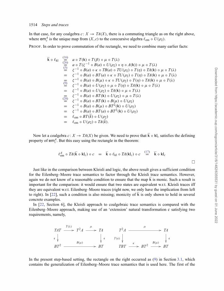
PROOF. In order to prove commutation of the rectangle, we need to combine many earlier facts:
k ◦ �kl(16)= a ◦ T(k) ◦ T(β) ◦ μ ◦ T(λ)(26)= a ◦ T(ζ−1 ◦ B(a) ◦ U(ρ2) ◦ η ◦ A(k)) ◦ μ ◦ T(λ)(5)= ζ−1 ◦ B(a) ◦ κ ◦ TB(a) ◦ TU(ρ2) ◦ T(η) ◦ TA(k) ◦ μ ◦ T(λ)
= ζ−1 ◦ B(a) ◦ BT(a) ◦ κ ◦ TU(ρ2) ◦ T(η) ◦ TA(k) ◦ μ ◦ T(λ)
= ζ−1 ◦ B(a) ◦ B(μ) ◦ κ ◦ TU(ρ2) ◦ T(η) ◦ TA(k) ◦ μ ◦ T(λ)(9)= ζ−1 ◦ B(a) ◦ U(ρ2) ◦ μ ◦ T(η) ◦ TA(k) ◦ μ ◦ T(λ)
= ζ−1 ◦ B(a) ◦ U(ρ2) ◦ TA(k) ◦ μ ◦ T(λ)
= ζ−1 ◦ B(a) ◦ BT(k) ◦ U(ρ2) ◦ μ ◦ T(λ)(28)= ζ−1 ◦ B(a) ◦ BT(k) ◦ B(μ) ◦ U(ρ2)
= ζ−1 ◦ B(a) ◦ B(μ) ◦ BT2(k) ◦ U(ρ2)
= ζ−1 ◦ B(a) ◦ BT(a) ◦ BT2(k) ◦ U(ρ2)
= �em ◦ BT(k) ◦ U(ρ2)
= �em ◦ U(ρ2) ◦ TA(k).
Now let a coalgebra c : X → TA(X ) be given. We need to prove that k ◦ klc satisfies the definingproperty of emA
c . But this easy using the rectangle in the theorem:
�Aem ◦ TA(k ◦ klc) ◦ c = k ◦ �kl ◦ TA(klc) ◦ c
(17)= k ◦ klc
�Just like in the comparison between Kleisli and logic, the above result gives a sufficient condition
for the Eilenberg–Moore trace semantics to factor through the Kleisli trace semantics. However,again we do not know of a reasonable condition to ensure that the map k is monic. Such a result isimportant for the comparison: it would ensure that two states are equivalent w.r.t. Kleisli traces iffthey are equivalent w.r.t. Eilenberg–Moore traces (right now, we only have the implication from leftto right). In [22], such a condition is also missing; monicity of k is only shown to hold in severalconcrete examples.
In [22, Section 6], the Kleisli approach to coalgebraic trace semantics is compared with theEilenberg–Moore approach, making use of an ‘extension’ natural transformation e satisfying tworequirements, namely,
In the present step-based setting, the rectangle on the right occurred as (9) in Section 3.1, whichcontains the generalization of Eilenberg–Moore trace semantics that is used here. The first of the
Dow
nloaded from https://academ
ic.oup.com/logcom
/article/31/6/1482/6355531 by guest on 01 June 2022
Steps and traces 1515
above two rectangles captures compatibility in Proposition 7.12 and is used for a comparison ofKleisli and Eilenberg–Moore semantics in Theorem 7.13. The conclusion is that the approach ofthis paper not only covers the approach of [22, Section 6] but also puts it in a wider step-basedperspective, using corecursive algebras.
8 Completely iterative algebras
Milius [37] introduced a notion of ‘complete iterativity’ of algebras that is stronger than corecursive-ness and has the advantage of being preserved by various constructions. So, whenever we encountera corecursive algebra, it is natural to ask whether it is in fact completely iterative. This section showsthat all our corecursive algebras are completely iterative (Theorem 8.3), and that this yields tracemaps in more general settings.
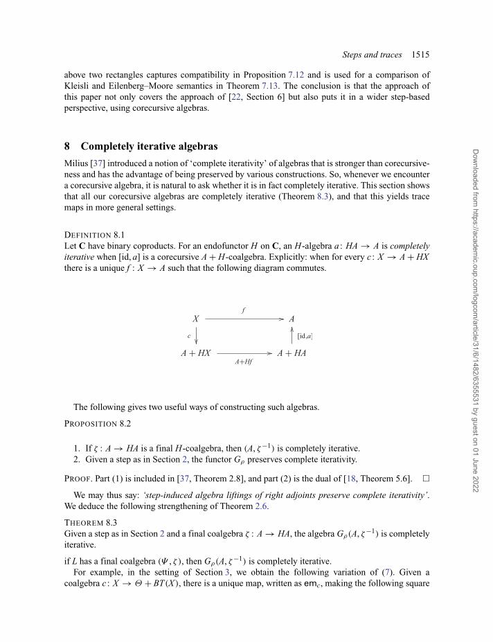
DEFINITION 8.1Let C have binary coproducts. For an endofunctor H on C, an H-algebra a : HA → A is completelyiterative when [id, a] is a corecursive A + H-coalgebra. Explicitly: when for every c : X → A + HXthere is a unique f : X → A such that the following diagram commutes.
The following gives two useful ways of constructing such algebras.
PROPOSITION 8.2
1. If ζ : A → HA is a final H-coalgebra, then (A, ζ−1) is completely iterative.2. Given a step as in Section 2, the functor Gρ preserves complete iterativity.
PROOF. Part (1) is included in [37, Theorem 2.8], and part (2) is the dual of [18, Theorem 5.6]. �We may thus say: ‘step-induced algebra liftings of right adjoints preserve complete iterativity’.
We deduce the following strengthening of Theorem 2.6.
THEOREM 8.3Given a step as in Section 2 and a final coalgebra ζ : A → HA, the algebra Gρ(A, ζ−1) is completelyiterative.
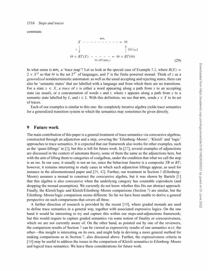
if L has a final coalgebra (Ψ , ζ ), then Gρ(A, ζ−1) is completely iterative.For example, in the setting of Section 3, we obtain the following variation of (7). Given a
coalgebra c : X → Θ + BT(X ), there is a unique map, written as emc, making the following square
Dow
nloaded from https://academ
ic.oup.com/logcom
/article/31/6/1482/6355531 by guest on 01 June 2022
1516 Steps and traces
commute:
(29)
In what sense is emc a ‘trace map’? Let us look at the special case of Example 3.2, where B(X ) =2 × X A so that Θ is the set 2A∗
of languages, and T is the finite powerset monad. Think of c as ageneralized nondeterministic automaton: as well as the usual accepting and rejecting states, there canalso be ‘semantic states’ that are labelled with a language and from which there are no transitions.For a state x ∈ X , a trace of x is either a word appearing along a path from x to an acceptingstate (as usual), or a concatenation of words s and t, where s appears along a path from x to asemantic state labelled by L, and t ∈ L. With this definition, we see that emc sends x ∈ X to its setof traces.
Each of our examples is similar to this one: the completely iterative algebra yields trace semanticsfor a generalized transition system in which the semantics may sometimes be given directly.
9 Future work
The main contribution of this paper is a general treatment of trace semantics via corecursive algebras,constructed through an adjunction and a step, covering the ‘Eilenberg–Moore’, ‘Kleisli’ and ‘logic’approaches to trace semantics. It is expected that our framework also works for other examples, suchas the ‘quasi-liftings’ in [2], but this is left for future work. In [27], several examples of adjunctionsare discussed in the context of automata theory, some of them the same as the adjunctions here, butwith the aim of lifting them to categories of coalgebras, under the condition that what we call the stepis an iso. In our case, it usually is not an iso, since the behaviour functor is a composite TB or BT ;however, it remains interesting to study cases in which such adjunction liftings appear, as used forinstance in the aforementioned paper and [29, 42]. Further, our treatment in Section 3 (Eilenberg–Moore) assumes a monad to construct the corecursive algebra, but it was shown by Bartels [1]that this algebra is also corecursive when the underlying category has countable coproducts (anddropping the monad assumption). We currently do not know whether this fits our abstract approach.Finally, the Kleisli/logic and Kleisli/Eilenberg–Moore comparisons (Section 7) are similar, but theEilenberg–Moore/logic comparison seems different. So far we have been unable to derive a generalperspective on such comparisons that covers all three.
A further direction of research is provided by the recent [10], where graded monads are usedto define trace semantics in a general way, together with associated expressive logics. On the onehand it would be interesting to try and capture this within our steps-and-adjunctions framework;but this would require to capture graded semantics via some notion of finality or corecursiveness,which we are not currently aware of. On the other hand, as pointed out by one of the reviewers,the comparison results of Section 7 can be viewed as expressivity results of one semantics w.r.t. theother—this insight is interesting on its own, and might help in devising a more general method formaking comparisons as in Section 7, also discussed above. Further, the expressiveness criteria in[10] may be useful to address the issues in the comparison of Kleisli semantics to Eilenberg–Mooreand logical trace semantics. We leave these considerations for future work.
Dow
nloaded from https://academ
ic.oup.com/logcom
/article/31/6/1482/6355531 by guest on 01 June 2022
Steps and traces 1517
Funding
The research leading to these results has received funding from the European Research Council underthe European Union’s Seventh Framework Programme (FP7/2007-2013)/ERC grant agreement nr.320571.
Acknowledgements
We are grateful to the anonymous referees of both the conference version and this extended paperfor various comments and suggestions.
References[1] F. Bartels. Generalised coinduction. Mathematical Structures in Computer Science, 13, 321–
348, 2003.[2] F. Bonchi, A. Silva and A. Sokolova. The power of convex algebras. In CONCUR, pp. 23:1–
23:18. Vol. 85 of LIPIcs. Schloss Dagstuhl—Leibniz-Zentrum für Informatik, 2017.[3] M. M. Bonsangue and A. Kurz. Duality for logics of transition systems. In FoSSaCS, pp. 455–
469. Vol. 3441 of Lect. Notes Comp. Sci. Springer, 2005.[4] M. M. Bonsangue, S. Milius and A. Silva. Sound and complete axiomatizations of coalgebraic
language equivalence. ACM Transactions on Computational Logic, 14, 7:1–7:52, 2013.[5] N. J. Bowler, P. B. Levy and G. D. Plotkin. Initial algebras and final coalgebras consisting of
nondeterministic finite trace strategies. In MFPS, pp. 23–44. Vol. 341 of Elect. Notes in Theor.Comp. Sci. Elsevier, 2018.
[6] V. Capretta, T. Uustalu and V. Vene. Recursive coalgebras from comonads. Information andComputation, 204, 437–468, 2006.
[7] V. Capretta, T. Uustalu and V. V. C. algebras. A study of general structured corecursion. InSBMF, pp. 84–100. Vol. 5902 of Lect. Notes Comp. Sci. Springer, 2009.
[8] L.-T. Chen and A. Jung. On a categorical framework for coalgebraic modal logic. ElectronicNotes in Theoretical Computer Science, 308, 109–128, 2014.
[9] C. Cîrstea. A coalgebraic approach to quantitative linear time logics. CoRR, abs/1612.07844,2016. https://arxiv.org/abs/1612.07844v1.
[10] U. Dorsch, S. Milius and L. Schröder. Graded monads and graded logics for the lineartime—branching time spectrum. In CONCUR, pp. 36:1–36:16. Vol. 140 of LIPIcs. SchlossDagstuhl—Leibniz-Zentrum für Informatik, 2019.
[11] A. Eppendahl. Coalgebra-to-algebra morphisms. Electronic Notes in Theoretical ComputerScience, 29, 42–49, 1999.
[12] J. Y. Girard, Y. Lafont and P. Taylor. Proofs and Types. Vol. 7 of Cambridge Tracts inTheoretical Computer Science. Cambridge University Press, 1988.
[13] S. Goncharov. Trace semantics via generic observations. In CALCO, pp. 158–174. Vol. 8089of Lect. Notes Comp. Sci. Springer, 2013.
[14] P. Hancock and P. Hyvernat. Programming interfaces and basic topology. Annals of Pure andApplied Logic, 137, 189–239, 05 2009.
[15] I. Hasuo. Generic weakest precondition semantics from monads enriched with order. Theoret-ical Computer Science, 604, 2–29, 2015.
[16] I. Hasuo, B. Jacobs and A. Sokolova. Generic trace semantics via coinduction. Logical Methodsin Computer Science, 3, 2007.
Dow
nloaded from https://academ
ic.oup.com/logcom
/article/31/6/1482/6355531 by guest on 01 June 2022
1518 Steps and traces
[17] W. Hino, H. Kobayashi, I. Hasuo and B. Jacobs. Healthiness from duality. In LICS. IEEE,Computer Science Press, 2016.
[18] R. Hinze, N. Wu and J. Gibbons. Conjugate hylomorphisms—or: the mother of all structuredrecursion schemes. In POPL, pp. 527–538. ACM, 2015.
[19] B. Jacobs. A bialgebraic review of deterministic automata, regular expressions and languages.In Essays Dedicated to Joseph A. Goguen, pp. 375–404. Vol. 4060 of Lect. Notes Comp. Sci.Springer, 2006.
[20] B. Jacobs. A recipe for state and effect triangles. Logical Methods in Computer Science, 13,2017.
[21] B. Jacobs, P. Levy and J. Rot. Steps and traces. In CMCS, pp. 122–143. Vol. 11202 of Lect.Notes Comp. Sci. Springer, 2018.
[22] B. Jacobs, A. Silva and A. Sokolova. Trace semantics via determinization. Journal of Computerand System Sciences, 81, 859–879, 2015.
[23] B. Jacobs and A. Sokolova. Exemplaric expressivity of modal logics. Journal of Logic andComputation, 20, 1041–1068, 2010.
[24] R. Jagadeesan, C. Pitcher and J. Riely. Open bisimulation for aspects. In AOSD,pp. 107–120. Vol. 208 of ACM International Conference Proceeding Series. ACM,2007.
[25] P. Johnstone. Adjoint lifting theorems for categories of algebras. Bulletin of the LondonMathematical Society, 7, 294–297, 1975.
[26] G. M. Kelly and R. Street. Review of the elements of 2-categories. In Category Seminar:Proceedings Sydney Category Seminar 1972/1973, G. M. Kelly, ed. Vol. 420 in Lecture Notesin Mathematics. Springer, 1974.
[27] H. Kerstan, B. König and B. Westerbaan. Lifting adjunctions to coalgebras to (re)discoverautomata constructions. In CMCS, pp. 168–188. Vol. 8446 of Lect. Notes Comp. Sci. Springer,2014.
[28] B. Klin. Coalgebraic modal logic beyond sets. In MFPS, M. Fiore, ed. Vol. 173 in Elect. Notesin Theor. Comp. Sci. Elsevier, Amsterdam, 2007.
[29] B. Klin and J. Rot. Coalgebraic trace semantics via forgetful logics. Logical Methods inComputer Science, 12, 2016.
[30] B. Klin and J. Salamanca. Iterated covariant powerset is not a monad. Electronic Notes inTheoretical Computer Science, 341, 261–276, 2018.
[31] A. Kurz, S. Milius, D. Pattinson and L. Schröder. Simplified coalgebraic trace equivalence.In Software, Services, and Systems, pp. 75–90. Vol. 8950 of Lect. Notes Comp. Sci. Springer,2015.
[32] J. Laird. A fully abstract trace semantics for general references. In ICALP, pp. 667–679. Vol.4596 of Lect. Notes Comp. Sci. Springer, 2007.
[33] S. B. Lassen and P. B. Levy. Typed normal form bisimulation. In CSL, pp. 283–297. Vol. 4646of Lect. Notes Comp. Sci. Springer, 2007.
[34] T. Leinster. Higher Operads, Higher Categories. Vol. 298 of London Mathematical SocietyLecture Notes. Cambridge University Press, 2004.
[35] P. B. Levy. Final coalgebras from corecursive algebras. In CALCO, pp. 221–237. Vol. 35 ofLIPIcs. Schloss Dagstuhl—Leibniz-Zentrum für Informatik, 2015.
[36] P. B. Levy and S. Staton. Transition systems over games. In CSL-LICS, pp. 64:1–64:10. ACM,2014.
[37] S. Milius. Completely iterative algebras and completely iterative monads. Information andComputation, 196, 1–41, 2005.
Dow
nloaded from https://academ
ic.oup.com/logcom
/article/31/6/1482/6355531 by guest on 01 June 2022
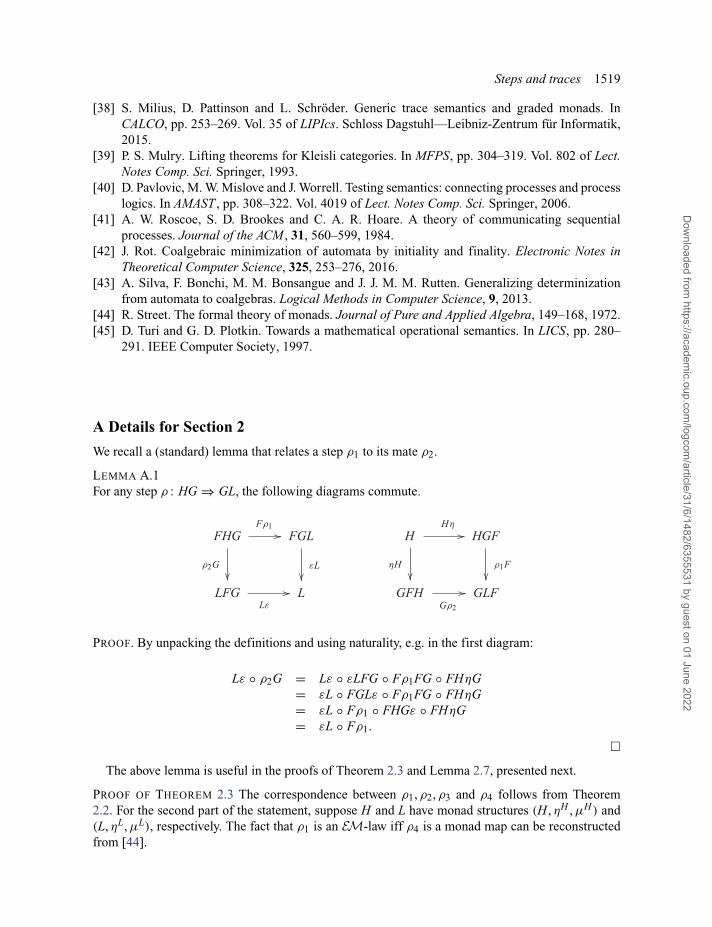
Steps and traces 1519
[38] S. Milius, D. Pattinson and L. Schröder. Generic trace semantics and graded monads. InCALCO, pp. 253–269. Vol. 35 of LIPIcs. Schloss Dagstuhl—Leibniz-Zentrum für Informatik,2015.
[39] P. S. Mulry. Lifting theorems for Kleisli categories. In MFPS, pp. 304–319. Vol. 802 of Lect.Notes Comp. Sci. Springer, 1993.
[40] D. Pavlovic, M. W. Mislove and J. Worrell. Testing semantics: connecting processes and processlogics. In AMAST , pp. 308–322. Vol. 4019 of Lect. Notes Comp. Sci. Springer, 2006.
[41] A. W. Roscoe, S. D. Brookes and C. A. R. Hoare. A theory of communicating sequentialprocesses. Journal of the ACM , 31, 560–599, 1984.
[42] J. Rot. Coalgebraic minimization of automata by initiality and finality. Electronic Notes inTheoretical Computer Science, 325, 253–276, 2016.
[43] A. Silva, F. Bonchi, M. M. Bonsangue and J. J. M. M. Rutten. Generalizing determinizationfrom automata to coalgebras. Logical Methods in Computer Science, 9, 2013.
[44] R. Street. The formal theory of monads. Journal of Pure and Applied Algebra, 149–168, 1972.[45] D. Turi and G. D. Plotkin. Towards a mathematical operational semantics. In LICS, pp. 280–
291. IEEE Computer Society, 1997.
A Details for Section 2
We recall a (standard) lemma that relates a step ρ1 to its mate ρ2.
LEMMA A.1For any step ρ : HG ⇒ GL, the following diagrams commute.
PROOF. By unpacking the definitions and using naturality, e.g. in the first diagram:
Lε ◦ ρ2G = Lε ◦ εLFG ◦ Fρ1FG ◦ FHηG= εL ◦ FGLε ◦ Fρ1FG ◦ FHηG= εL ◦ Fρ1 ◦ FHGε ◦ FHηG= εL ◦ Fρ1.
�The above lemma is useful in the proofs of Theorem 2.3 and Lemma 2.7, presented next.
PROOF OF THEOREM 2.3 The correspondence between ρ1, ρ2, ρ3 and ρ4 follows from Theorem2.2. For the second part of the statement, suppose H and L have monad structures (H , ηH , μH ) and(L, ηL, μL), respectively. The fact that ρ1 is an EM-law iff ρ4 is a monad map can be reconstructedfrom [44].
Dow
nloaded from https://academ
ic.oup.com/logcom
/article/31/6/1482/6355531 by guest on 01 June 2022
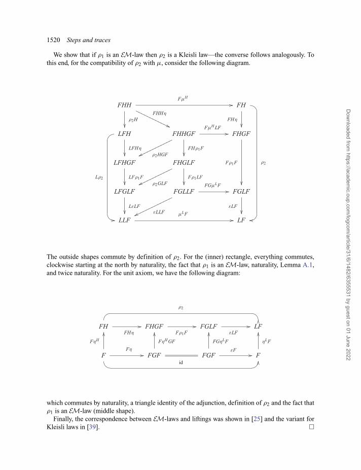
1520 Steps and traces
We show that if ρ1 is an EM-law then ρ2 is a Kleisli law—the converse follows analogously. Tothis end, for the compatibility of ρ2 with μ, consider the following diagram.
The outside shapes commute by definition of ρ2. For the (inner) rectangle, everything commutes,clockwise starting at the north by naturality, the fact that ρ1 is an EM-law, naturality, Lemma A.1,and twice naturality. For the unit axiom, we have the following diagram:
which commutes by naturality, a triangle identity of the adjunction, definition of ρ2 and the fact thatρ1 is an EM-law (middle shape).
Finally, the correspondence between EM-laws and liftings was shown in [25] and the variant forKleisli laws in [39]. �
Dow
nloaded from https://academ
ic.oup.com/logcom
/article/31/6/1482/6355531 by guest on 01 June 2022
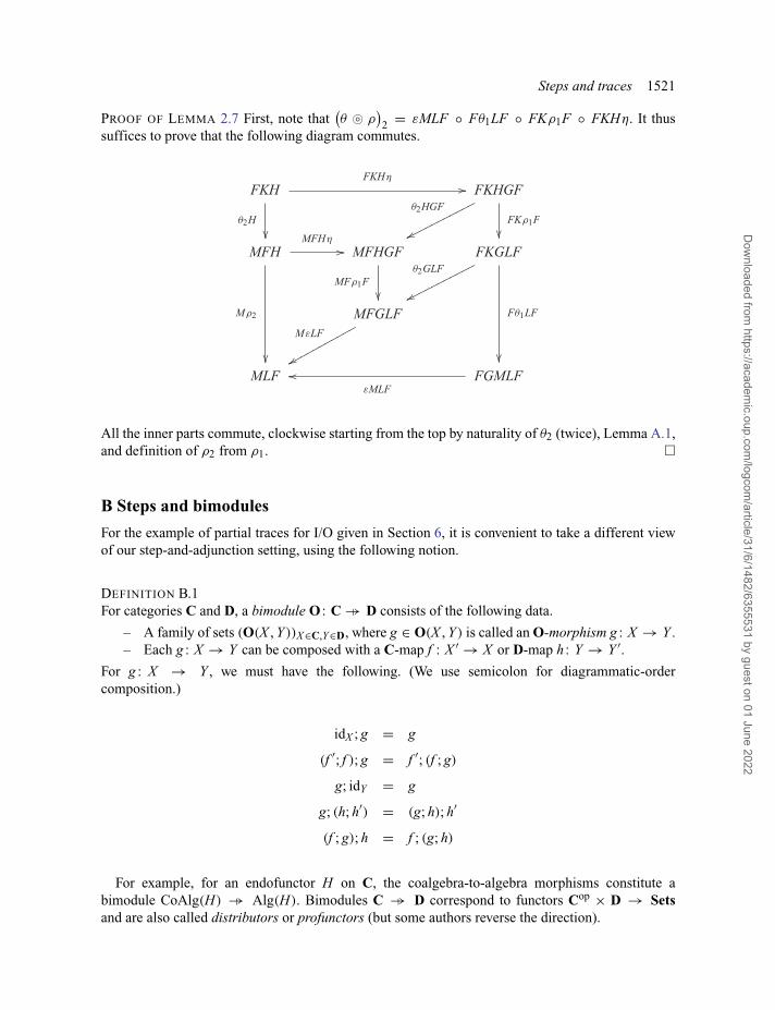
Steps and traces 1521
PROOF OF LEMMA 2.7 First, note that(θ � ρ
)2 = εMLF ◦ Fθ1LF ◦ FKρ1F ◦ FKHη. It thus
suffices to prove that the following diagram commutes.
All the inner parts commute, clockwise starting from the top by naturality of θ2 (twice), Lemma A.1,and definition of ρ2 from ρ1. �
B Steps and bimodules
For the example of partial traces for I/O given in Section 6, it is convenient to take a different viewof our step-and-adjunction setting, using the following notion.
DEFINITION B.1For categories C and D, a bimodule O : C →� D consists of the following data.
– A family of sets (O(X , Y ))X∈C,Y∈D, where g ∈ O(X , Y ) is called an O-morphism g : X → Y .– Each g : X → Y can be composed with a C-map f : X ′ → X or D-map h : Y → Y ′.
For g : X → Y , we must have the following. (We use semicolon for diagrammatic-ordercomposition.)
idX ; g = g
(f ′; f ); g = f ′; (f ; g)
g; idY = g
g; (h; h′) = (g; h); h′
(f ; g); h = f ; (g; h)
For example, for an endofunctor H on C, the coalgebra-to-algebra morphisms constitute abimodule CoAlg(H) →� Alg(H). Bimodules C →� D correspond to functors Cop × D → Setsand are also called distributors or profunctors (but some authors reverse the direction).
Dow
nloaded from https://academ
ic.oup.com/logcom
/article/31/6/1482/6355531 by guest on 01 June 2022

1522 Steps and traces
DEFINITION B.2
1. A map of bimodules
sends each O-morphism g : X → Y to an O′-morphism Rg : X → Y with the followingcommuting:
2. More generally, a 2-cell
sends each O-morphism g : X → Y to an O′-morphism Rg : HX → LY with the followingcommuting:
The product construction on categories extends to bimodules:
DEFINITION B.3Let (Oj : Cj →� Dj)j∈J be a family of bimodules. Then the bimodule
∏j∈J Oj :
∏j∈J Cj →� ∏
j∈J Djis defined by saying that a morphism (Xj)j∈J → (Yj)j∈J is a family (gj : Xj → Yj)j∈J , where gj is anOj-morphism for all j ∈ J . Composition is defined componentwise.
Of course this construction extends also to maps and 2-cells between bimodules.Here are two ways of constructing a bimodule C →� D.
Dow
nloaded from https://academ
ic.oup.com/logcom
/article/31/6/1482/6355531 by guest on 01 June 2022
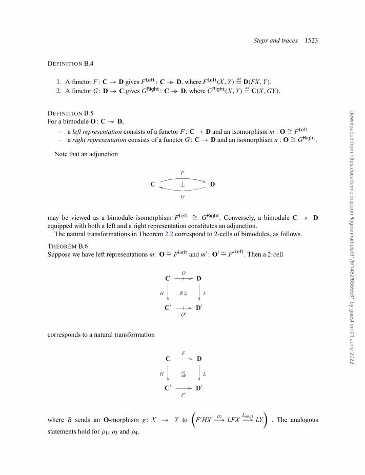
Steps and traces 1523
DEFINITION B.4
1. A functor F : C → D gives FLeft : C →� D, where FLeft(X , Y )def= D(FX , Y ).
2. A functor G : D → C gives GRight : C →� D, where GRight(X , Y )def= C(X , GY ).
DEFINITION B.5For a bimodule O : C →� D,
– a left representation consists of a functor F : C → D and an isomorphism m : O ∼= FLeft
– a right representation consists of a functor G : C → D and an isomorphism n : O ∼= GRight.
Note that an adjunction
may be viewed as a bimodule isomorphism FLeft ∼= GRight. Conversely, a bimodule C →� Dequipped with both a left and a right representation constitutes an adjunction.
The natural transformations in Theorem 2.2 correspond to 2-cells of bimodules, as follows.
THEOREM B.6Suppose we have left representations m : O ∼= FLeft and m′ : O′ ∼= F′Left. Then a 2-cell
corresponds to a natural transformation
where R sends an O-morphism g : X → Y to(
F′HXρ2−→ LFX
Lm(g)−→ LY
). The analogous
statements hold for ρ1, ρ3 and ρ4.
Dow
nloaded from https://academ
ic.oup.com/logcom
/article/31/6/1482/6355531 by guest on 01 June 2022
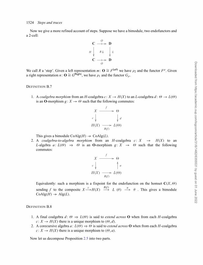
1524 Steps and traces
Now we give a more refined account of steps. Suppose we have a bimodule, two endofunctors anda 2-cell:
We call R a ‘step’. Given a left representation m : O ∼= FLeft we have ρ2 and the functor Fρ . Givena right representation n : O ∼= GRight, we have ρ1 and the functor Gρ .
DEFINITION B.7
1. A coalgebra morphism from an H-coalgebra c : X → H(X ) to an L-coalgebra d : Θ → L(Θ)
is an O-morphism g : X → Θ such that the following commutes:
This gives a bimodule CoAlg(H) →� CoAlg(L).2. A coalgebra-to-algebra morphism from an H-coalgebra c : X → H(X ) to an
L-algebra a : L(Θ) ⇒ Θ is an O-morphism g : X → Θ such that the followingcommutes:
Equivalently: such a morphism is a fixpoint for the endofunction on the homset C(X , Θ)
sending f to the composite Xc−→H(X )
R(f )−→ L (θ)a−→ θ . This gives a bimodule
CoAlg(H) →� Alg(L).
DEFINITION B.8
1. A final coalgebra d : Θ ⇒ L(Θ) is said to extend across O when from each H-coalgebrac : X → H(X ) there is a unique morphism to (Θ , d).
2. A corecursive algebra a : L(Θ) ⇒ Θ is said to extend across O when from each H-coalgebrac : X → H(X ) there is a unique morphism to (Θ , a).
Now let us decompose Proposition 2.5 into two parts.
Dow
nloaded from https://academ
ic.oup.com/logcom
/article/31/6/1482/6355531 by guest on 01 June 2022
Steps and traces 1525
PROPOSITION B.9
1. Let O have a left representation m : O ∼= FLeft. Then any corecursive L-algebra (Θ , a) extendsacross O. (And hence also any final L-algebra.) Explicitly, the map (X , c) → (Θ , a) is m−1
applied to the map Fρ(X , c) → (Θ , a).2. Let O have a right representation n : O ∼= GRight. Then any corecursive L-algebra (Θ , a)
extending across O is sent by Gρ to a corecursive H-algebra. Explicitly, the map (X , c) →Gρ(Θ , a) is n applied to the map (X , c) → (Θ , a).
Note that this story also appears, in contravariant form, in [35, Propositions 16–17].
Received 27 January 2019
Dow
nloaded from https://academ
ic.oup.com/logcom
/article/31/6/1482/6355531 by guest on 01 June 2022


