Embed Size (px)
Citation preview
arX
iv:a
stro
-ph/
0205
202v
1 1
4 M
ay 2
002
Inflation and non–Gaussianity
Alejandro Gangui∗
Instituto de Astronomıa y Fısica del Espacio, Ciudad Universitaria, 1428 Buenos Aires, Argentina, and
Dept. de Fısica, Universidad de Buenos Aires, Ciudad Universitaria – Pab. 1, 1428 Buenos Aires, Argentina.
Jerome Martin†
Institut d’Astrophysique de Paris, 98bis boulevard Arago, 75014 Paris, France.
Mairi Sakellariadou‡
Department of Astrophysics, Astronomy, and Mechanics,
University of Athens, Panepistimiopolis, GR-15784 Zografos, Hellas, and
Institut d’Astrophysique de Paris, 98bis boulevard Arago, 75014 Paris, France.
(Dated: February 1, 2008)
We study non-Gaussian signatures on the cosmic microwave background (CMB) radiation pre-dicted within inflationary models with non-vacuum initial states for cosmological perturbations.The model incorporates a privileged scale, which implies the existence of a feature in the primordialpower spectrum. This broken-scale-invariant model predicts a vanishing three-point correlation func-tion for the CMB temperature anisotropies (or any other odd-numbered-point correlation function)whilst an intrinsic non-Gaussian signature arises for any even-numbered-point correlation function.We thus focus on the first non-vanishing moment, the CMB four-point function at zero lag, namelythe kurtosis, and compute its expected value for different locations of the primordial feature in thespectrum, as suggested in the literature to conform to observations of large scale structure. Theexcess kurtosis is found to be negative and the signal to noise ratio for the dimensionless excesskurtosis parameter is equal to |S/N | ≃ 4 × 10⁻⁴, almost independently of the free parameters ofthe model. This signature turns out to be undetectable. We conclude that, subject to current tests,Gaussianity is a generic property of single field inflationary models. The only uncertainty concern-ing this prediction is that the effect of back-reaction has not yet been properly incorporated. Theimplications for the trans-Planckian problem of inflation are also briefly discussed.
PACS numbers: 98.80.Cq, 98.70.Vc
I. INTRODUCTION
The theory of inflation is presently the most appealing candidate for describing the early universe. Inflationessentially consists of a phase of accelerated expansion which took place at a very high energy scale. One of the mainreasons for such an appeal is the fact that inflation is deeply rooted in the basic principles of general relativity andfield theory, which are well-tested theories. It is because all the forms of energy gravitate in general relativity thatone of them, the pressure, which can be negative in field theory, is able to cause the acceleration in the expansionof the universe. In addition, when the principles of quantum mechanics are taken into account, inflation providesa natural explanation for the origin of the large scale structures and the associated temperature anisotropies in theCosmic Microwave Background (CMB) radiation [1].
Inflation makes four key predictions: (i) the curvature of the space-like sections vanishes, i.e. the total energy density,relative to the critical density, is Ω0 = 1, (ii) the power spectrum of density fluctuations is almost scale invariant,i.e. its spectral index is n
S≃ 1, (iii) there is a background of primordial gravitational waves (which is also scale
invariant), and (iv) the statistical properties of the CMB are Gaussian. In this article we focus on the last predictionand investigate whether it is a robust and generic property of inflationary models. The statistical properties of theCMB will be measured with high accuracy by the MAP and Planck satellites [2]. So far the preliminary measurementsof the three- and four-point correlation functions [3, 4, 5] seem to be consistent with Gaussianity.
The fact that the statistical properties of the CMB are Gaussian can be directly traced back to the commonassumption that the quantum fluctuations of the inflaton field are placed in the vacuum state [6]. Therefore, in
∗Electronic address: [email protected]†Electronic address: [email protected]‡Electronic address: [email protected], [email protected]
2
order to answer the above question, one has to investigate which kind of non-Gaussianity shows up if the vacuumstate assumption is relaxed [7, 8, 9, 10]. In particular, one crucial point is to study whether this modification yieldsa detectable signal for future CMB or large-scale structure observations. Let us also notice that there exist othermechanisms to produce non-Gaussianity within the framework of inflation. Some of them have been studied inRefs. [11, 12].
Assuming that the quantum state of the perturbations is a non-vacuum state immediately leads to the followingdifficulty: non-vacuum initial states imply, in general, a large energy density of inflaton field quanta, not of a cosmo-logical term type [13]. In other words, generically, if the initial state is not the vacuum then there is a back-reactionproblem that could upset the inflationary phase. However, as we will argue below, one cannot directly conclude thatthis would prevent inflation from occurring altogether because, without a detailed calculation, it is difficult to guesswhat the back-reaction effect on the background would be. Such a detailed calculation is in principle possible bymeans of the formalism developed in Ref. [14]. To our knowledge, such a computation has never been performed. Thecalculation of second order effects is clearly a complicated issue and is still the subject of discussions in the literature,see [15] for example. Moreover there exist situations where it can be avoided, and this is in fact the case if the numberof e-folds is not too large. In this article, we will not address the general question mentioned above but will ratherconcentrate on the more modest aim of calculating the non-Gaussianity in a case where the back-reaction problem isnot too severe, hoping in this way to capture some features of the real situation.
There exist other arguments to study the non-Gaussianity that arises from a non-vacuum state. One of these isthe so-called trans-Planckian problem of inflation [16]: the quantum fluctuations are typically generated from sub-Planckian scales and therefore the predictions of inflation depend in fact on hidden assumptions about the physicson length scales smaller than the Planck scale. However, it has recently been shown that inflation is robust to somechanges of the standard laws of physics beyond the Planck scale. More precisely, inflation is robust to a modification ofthe dispersion relation, at least if those changes are not too drastic, in practice if the Wigner-Kramer-Brillouin (WKB)evolution of the cosmological perturbations is preserved. However, modeling trans-Planckian physics by a change inthe dispersion relation is clearly ad-hoc. Therefore, it is interesting to consider other possibilities; for example, onecould imagine that the inflaton field emerges from the trans-Planckian regime in a non-vacuum state. Non-Gaussianitywould then be, in this case, a signature of non standard physics and it seems to us interesting to quantify this effect.Let us note that similar ideas have been suggested in Ref. [17] in a slightly different context. Let us also remark thatit has been shown recently in Ref. [18] that placing the cosmological perturbations in a non-vacuum state would leadto possible observable effects, for instance a modification of the consistency check of inflation.
Another motivation for calculating non-Gaussianity when the initial state is not the vacuum is that this modelcould be used to test the methods that are being developed to detect non-Gaussianity in the future CMB maps.There have been approaches based on the nth order moments or the cumulants of the temperature distribution [19],the n-point correlation functions or their spherical harmonic transforms [20], and also works based on the detection ofgradients in the wavelet space [21], to mention just a few methods. In the last approach, namely the wavelet analysisof a signal [21], the test maps which were employed were characterized by a non-skewed non-Gaussian distribution.Therefore, any non-Gaussianity was indicated by a non-zero excess kurtosis of the coefficients associated with thegradients of the signal. As we will show, this is exactly our case. This wavelet analysis of a signal was then applied [22]to search for the CMB non-Gaussian signatures. More precisely, these authors investigated the detectability of a non-Gaussian signal induced by secondary anisotropies, while assuming Gaussian-distributed primary anisotropies. Theirmethod [22] is unable to detect such non-Gaussianity for the MAP-like instrumental configuration while it can do itfor Planck-like capabilities.
From the theoretical point of view the simplest way to generalize the vacuum initial state, which contains noprivileged scale, is to consider an initial state with a built-in characteristic scale, kb [8]. Here, we will consider a non-vacuum state which is simpler and more generic than the one considered in this previous work. Several observablescan be used to constrain the parameter space. A first possibility is to use the CMB anisotropy multipole momentsto constrain the number of quanta n around the privileged scale. It has been shown in Ref. [8] that, typically, thisnumber cannot be large and in the present article we will always consider that n is a few. With the recent release ofthe BOOMERanG [23], MAXIMA [24] and DASI [25] data, which revealed the existence of a first acoustic peak inthe angular power spectrum at ℓ ∼ 200, followed by a second acoustic peak located at ℓ ∼ 500 and an evidence for athird peak, one can hope to obtain stronger constraints on kb and n very soon. Of course, another observable whichcan also be used is the matter density power spectrum. We will compare the predictions of our model for differentcosmologies with the result of recent observations below.
The model we are studying here belongs to a class with a Broken Scale Invariant (BSI) power spectrum for thematter density. Such a primordial spectrum could also be generated [26] during an inflationary era where the inflatonpotential is endowed with steps, e.g., induced by a spontaneous symmetry breaking phase transition. The mainmotivation behind this class of models comes from Abell/ACO galaxy cluster redshift surveys which indicate [27] thatthe matter power spectrum seems to contain large amplitude features close to a scale of 100h−1Mpc (see however
3
[28]). In support of this finding are the preliminary results of the recently released [29, 30] power spectrum analysis ofthe redshift surveys of Quasi-Stellar Objects (QSOs). Using the 10k catalogue from the 2dF QSO Redshift Survey [31],it has been tentatively identified [29] a “spike” feature at a scale ≈ 90h−1Mpc (≈ 65h−1Mpc) assuming a Lambdacontribution ΩΛ = 0.7 and an ordinary matter contribution Ωm = 0.3 (respectively, ΩΛ = 0 and Ωm = 1.0). Providedthis feature is confirmed, it might also have originated from acoustic oscillations in the tightly-coupled baryon-radiationfluid prior to decoupling. Using the CMBFAST code it was found [29] that this spike in the spectrum is seen at a≥ 25 per cent smaller wavenumber than the second acoustic peak, while higher values of the baryon contribution Ωb
may be needed to fit the amplitude of this feature. If we interpret this feature as originating from the primordialspectrum then, in order to be consistent with observations, the preferred scale kb must lie way below the horizontoday, possibly at a scale corresponding to the turn of the power spectrum [27] or at the scale matching the firstacoustic peak of the CMB temperature anisotropies [32]. One then sees that the presently available data alreadyrestricts the parameter space for the quantities kb and n [33].
For the class of models which contain a preferred scale, a generic prediction is that the three-point correlationfunction vanishes (as well as any higher-order odd-point function), whereas the four-point (as well as any higher-ordereven-point) correlation function no longer satisfies the relation
⟨(
δT
T
)4⟩
= 3
⟨(
δT
T
)2⟩2
, (1)
which is typical of Gaussian statistics. Since the third-order moment (the skewness) vanishes, a first step is tocalculate the fourth-order statistics (the kurtosis). It is interesting to perform this calculation for very large (COBE-size) angular scales, for which one can be confident that the source of non-Gaussianity is primordial. On the otherhand, if the non-Gaussian signature was calculated on intermediate scales, a stronger signal would be obtained;however, in that case the secondary sources would be more difficult to subtract and thus the transparency of the effectwould be compromised. To quantify the relevant amplitude of the signal, the excess kurtosis should be comparedwith its cosmic variance. This was computed, e.g., in Ref. [34], for a Gaussian field. Although, strictly speaking, oneshould compute the cosmic variance for the actual case and not rely on a mildly non-Gaussian analysis, the actualsmallness of the obtained signal largely justifies our approach.
We organize the rest of the paper as follows: in Section II, we discuss in detail the argument developed in Ref. [13]regarding the back-reaction problem. We show that any theory with a non-vacuum initial state has to face this issue.However, we also argue that it is not clear at all whether inflation will be prevented in this context. In Section III,we discuss our choice of a non-vacuum initial state for cosmological perturbations of quantum-mechanical origin andwe give some basic formulas for the two-point function. We calculate the CMB angular correlation function and theassociated matter power-spectrum for our choice of non-vacuum initial states, comparing the latter against currentobservations. In Section IV, we calculate the angular four-point correlation function and the related CMB excesskurtosis, while in Section V we discuss our results explicitly and present both analytical and full numerical estimatesof the normalized excess kurtosis for a typical case. In this Section we also compare this non-Gaussian signal withits corresponding cosmic variance. We round up with our conclusions in Section VII. In this paper, we use units suchthat c = 1.
II. INITIAL STATE FOR THE COSMOLOGICAL PERTURBATIONS AND THE BACK-REACTION
PROBLEM
In this Section we discuss the relevance of non-vacuum initial states for cosmological quantum perturbations. Theargument of Ref. [13] is based on the calculation of the energy density of the perturbed inflaton scalar field in a givennon-vacuum initial state. Since the perturbed inflaton and the Bardeen potential are linked through the Einsteinequations, it is clear that they should be placed in the same quantum state. Let us consider a quantum scalar fieldliving in a (spatially flat) Friedmann–Lemaıtre–Roberston–Walker background. The expression of the correspondingoperator reads
ϕ(η,x) =1
a(η)
1
(2π)3/2
∫
d3k1√2k
[
µk(η)ck(ηi)eik·x + µ∗
k(η)c†k(ηi)e−ik·x
]
, (2)
where ck(ηi) and c†k(ηi) are the annihilation and creation operators (respectively) satisfying the commutation relation
[ck, c†p] = δ(k−p), and where a(η) is the scale factor depending on conformal time η. The equation of motion for themode function µk(η) can be written as [35, 36, 37]
µ′′k +
(
k2 − a′′
a
)
µk = 0, (3)
4
where “primes” stand for derivatives with respect to conformal time. The above is the characteristic equation ofa parametric oscillator whose time-dependent frequency depends on the scale factor and its derivative. The energydensity and pressure for a scalar field are given by the following expressions
ρ =1
2a2ϕ′2 + V (ϕ) +
1
2a2δij∂iϕ∂jϕ, p =
1
2a2ϕ′2 − V (ϕ) − 1
6a2δij∂iϕ∂jϕ. (4)
Let us now calculate the energy and pressure in a state characterized by a distribution n(k) (giving the number n ofquanta with comoving wave-number k) for a free (i.e. V = 0) field. Let us denote such a state by |n(k)〉. Using somesimple algebra it is easy to find
〈n(k)|ρ|n(k)〉 =1
8π2a4
∫ +∞
0
dk
kk2
[
µ′kµ′∗
k − a′
a(µkµ′∗
k + µ∗kµ′
k) +
(
a′2
a2+ k2
)
µkµ∗k
]
(5)
+21
8π2a4
∫ +∞
0
dk
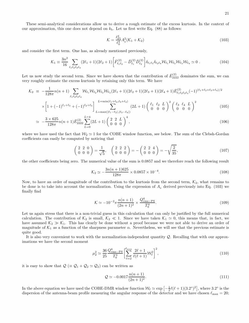
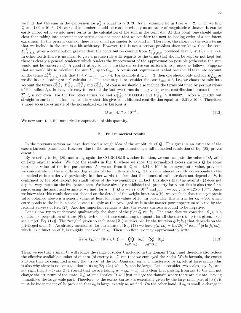
kk2n(k)
[
µ′kµ′∗
k − a′
a(µkµ′∗
k + µ∗kµ′
k) +
(
a′2
a2+ k2
)
µkµ∗k
]
, (6)
〈n(k)|p|n(k)〉 =1
8π2a4
∫ +∞
0
dk
kk2
[
µ′kµ′∗
k − a′
a(µkµ′∗
k + µ∗kµ′
k) +
(
a′2
a2− k2
3
)
µkµ∗k
]
(7)
+21
8π2a4
∫ +∞
0
dk
kk2n(k)
[
µ′kµ′∗
k − a′
a(µkµ′∗
k + µ∗kµ′
k) +
(
a′2
a2− k2
3
)
µkµ∗k
]
. (8)
We can evaluate these quantities in the high-frequency regime and take µk ≃ exp[−ik(η− ηi)], where ηi is some giveninitial conformal time. We get
〈n(k)|ρ|n(k)〉 =1
4π2a4
∫ +∞
0
dk
kk4 + 2
1
4π2a4
∫ +∞
0
dk
kk4n(k), (9)
〈n(k)|p|n(k)〉 =1
4π2a4
1
3
∫ +∞
0
dk
kk4 + 2
1
4π2a4
1
3
∫ +∞
0
dk
kk4n(k). (10)
Several comments are in order at this point. Firstly, the lower limit of the integral is certainly not zero because atsome fixed time, k → 0 corresponds to modes outside the horizon. So if we evaluate the previous integral at timeη then we should only integrate over those modes whose wavelength is smaller than the Hubble radius. But in theinfra-red sector, the integral is finite and so the contributions of those modes will be small. Therefore, in practicewe can keep a vanishing lower bound. Secondly, the first term of each expression is the contribution of the vacuum,i.e., is present even if n(k) = 0. This is clearly divergent in the ultra-violet regime. At this point, one should adopta regularization procedure (in curved space-time). Once this infinite vacuum contribution is subtracted out, ourrenormalized expressions for the density and pressure in the |n(k)〉 state read
〈n(k)|ρ|n(k)〉 =1
2π2a4
∫ +∞
0
dk
kk4n(k), 〈n(k)|p|n(k)〉 =
1
2π2a4
1
3
∫ +∞
0
dk
kk4n(k). (11)
For a well-behaved distribution function n(k) this result is finite. Thirdly, the perturbed inflaton (scalar) particlesbehave as radiation, as clearly indicated by the equation of state p = (1/3)ρ and as could have been guessed from thebeginning since the scalar field studied is free. To go further, we need to specify the function n(k). If we assume thatthe distribution n(k) is peaked around a value kb, it can be approximated by a constant distribution of n quanta,with n(kb) ≃ n, in the interval [kb − ∆k, kb + ∆k] centered around kb. If the interval is not too large, i.e. ∆k ≪ kb
then, at first order in ∆k/kb, we get
〈n(k)|ρ|n(k)〉 ≃ n
π2
∆k
kb
k4b
a4=
n
π2
∆k
kbH4
infe4Ne , (12)
where Ne is the number of e-folds counted back from the time of exit, see Fig 1. The time of exit is determined bythe condition kphys ≡ k/a ≃ Hinf , where Hinf is the Hubble parameter during inflation. It is simply related to thescale of inflation, Minf , by the relation Hinf ≃ M2
inf/mPl
. We have also assumed that, during inflation, the scale factorbehaves as a(t) ∝ exp(Hinf t). From Eq. (12), we see that the back-reaction problem occurs when one goes back intime since the energy density of the quanta scales as ≃ 1/a4. In this case, the number of e-folds Ne increases and thequantity 〈n(k)|ρ|n(k)〉 raises. This calculation is valid as long as 〈n(k)|ρ|n(k)〉 < ρinf = m2
PlH2
inf . When these twoquantities are equal, the energy density of the fluctuations is equal to the energy density of the background and thelinear theory breaks down. This happens for Ne = Nbr such that
Nbr ≃ 1
2ln
(
mPl
Hinf
)
, (13)
5
where we have assumed n∆k/(π2kb) ≃ O(1). Interestingly enough, this number does not depend on the scale k but
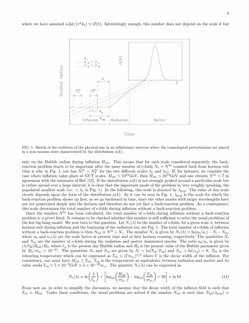
FIG. 1: Sketch of the evolution of the physical size in an inflationary universe where the cosmological perturbations are placedin a non-vacuum state characterized by the distribution n(k).
only on the Hubble radius during inflation Hinf . This means that for each scale considered separately, the back-reaction problem starts to be important after the same number of e-folds Ne = Nbr counted back from horizon exit(this is why in Fig. 1, one has Nbr
1 = Nbr3 for the two different scales λ1 and λ3). If, for instance, we consider the
case where inflation takes place at GUT scales, Minf ≃ 1016GeV, then Hinf ≃ 1013GeV and one obtains Nbr ≃ 7 inagreement with the estimates of Ref. [13]. If the distribution n(k) is not strongly peaked around a particular scale butis rather spread over a large interval, it is clear that the important mode of the problem is, very roughly speaking, thepopulated smallest scale (i.e. ≃ λ1 in Fig. 1). In the following, this scale is denoted by λpop. The value of this scaleclearly depends upon the form of the distribution n(k). As it can be seen in Fig. 1, λpop is the scale for which theback-reaction problem shows up first, as we go backward in time, since the other modes with larger wavelengths havenot yet penetrated deeply into the horizon and therefore do not yet face a back-reaction problem. As a consequence,this scale determines the total number of e-folds during inflation without a back-reaction problem.
Once the number Nbr has been calculated, the total number of e-folds during inflation without a back-reactionproblem is a priori fixed. It remains to be checked whether this number is still sufficient to solve the usual problems ofthe hot big bang model. We now turn to this question. Let N∗(λ) be the number of e-folds, for a given scale λ, betweenhorizon exit during inflation and the beginning of the radiation era, see Fig. 1. The total number of e-folds of inflationwithout a back-reaction problem is then Ninf ≡ Nbr + N∗. The number N∗ is given by N∗(λ) = ln(a0/a∗)−Nr −Nm,where a0 and a∗(λ) are the scale factor at present time and at first horizon crossing, respectively. The quantities Nr
and Nm are the number of e-folds during the radiation and matter dominated epochs. The ratio a0/a∗ is given by(λ/ℓH)Hinf/H0, where ℓ
His the present day Hubble radius and H0 is the present value of the Hubble parameter given
by H0/mPl
≃ 10−61. The quantities Nr and Nm are given by Nr = ln(Trh/Teq) and Nm ≃ ln(zeq) ≃ 9. Trh is the
reheating temperature which can be expressed as Trh ≃ (ΓmPl
)1/2 where Γ is the decay width of the inflaton. Forconsistency, one must have Minf ≥ Trh. Teq is the temperature at equivalence between radiation and matter and itsvalue reads Teq ≃ 5 × 10⁻⁹GeV ≃ 5 × 10⁻²⁸m
Pl. The quantity N∗(λ) can be expressed as
N∗(λ) ≃ ln
(
λ
ℓH
)
+
[
log10
(
Hinf
mPl
)
− log10
(
Trh
mPl
)
+ 29
]
× ln 10 . (14)
From now on, in order to simplify the discussion, we assume that the decay width of the inflaton field is such thatTrh ≃ Minf . Under these conditions, the usual problems are solved if the number Ninf is such that Ninf(λpop) ≃
6
ln(λpop/ℓH) + 29 × ln 10 > −4 + ln zend, where the quantity zend is the redshift at which the standard evolution (hot
big bang model) starts. It is linked to the reheating temperature by the relation log10(zend) ≃ 32 + log10(Trh/mPl
).This gives a constraint on the scale of inflation, namely
log10
(
Hinf
mPl
)
< 2 log10
(
λpop
ℓH
)
− 2.5 . (15)
It is known that inflation can take place between the TeV scale and the Planck scale which amounts to −32 <log10(Hinf/m
Pl) < 0. We see that the constraint given by Eq. (15) is not too restrictive. In particular, if we take
λpop = 0.1ℓH
and Hinf = 1013GeV, it is satisfied. However, if we decrease the scale λpop, the constraint becomes morerestrictive. The constraint derived in the present article appears to be less restrictive than in Ref. [13] because we donot assume that all scales are populated.
Another condition must be taken into account. We have seen that the duration of inflation without a back-reactionproblem is determined by the evolution of λpop. However, at the time at which the back-reaction problem showsup, one must also check that all the scales of astrophysical interest today were inside the horizon so that physicallymeaningful initial conditions can be chosen. This property is one of the most important advantages of the inflationaryscenario. If we say that the largest scale of interest today is the horizon, this condition is equivalent to
N∗(ℓH) < N∗(λpop) + Nbr ⇒ Nbr > ln
(
ℓH
λpop
)
. (16)
This condition is also not very restrictive, especially for large scales. As previously, the condition can be morerestrictive of one wants to populate smaller scales.
Before concluding this section, a last comment is in order. What is actually shown above is that, roughly Nbr
e-folds before the relevant mode left the horizon, we face a back-reaction problem, as the energy density of theperturbation 〈n(k)|ρ|n(k)〉 becomes of the same order of magnitude as the background ρ. So, before concluding thatnon-vacuum initial states may or may not turn off the inflationary phase, one should calculate the back-reaction effect,i.e., extend the present framework to second order as it was done in Ref. [14]. To our knowledge, this analysis is stillto be performed. Moreover, even if we take the most pessimistic position, that is, one in which we assume that theback-reaction of the perturbations on the background energy density prevents the inflationary phase, there still existmodels of inflation where the previous difficulties do not show up. Therefore, in the most pessimistic situation, thereis still a hope to reconcile non-vacuum initial states with inflation. Admittedly, the price to pay is a fine-tuning ofthe free parameters describing inflation and/or the non-vacuum state.
III. TWO-POINT CORRELATION FUNCTION FOR NON-VACUUM INITIAL STATES
A. General expressions
We now turn to consider the non-vacuum states for the cosmological perturbations of quantum mechanical origin.Let D(σ) be a domain in momentum space, such that if k is between 0 and σ, the domain D(σ) is filled by n quanta,while otherwise D contains nothing. Let us note that this domain is slightly different from the one considered inRef. [8]. The state |Ψ1(σ, n)〉 is defined by
|Ψ1(σ, n)〉 ≡∏
k∈D(σ)
(c†k)n
√n!
|0k〉⊗
p 6∈D(σ)
|0p〉 =⊗
k∈D(σ)
|nk〉⊗
p 6∈D(σ)
|0p〉. (17)
The state |nk〉 is an n-particle state satisfying, at conformal time η = ηi: ck|nk〉 =√
n|(n − 1)k〉 and c†k|nk〉 =√n + 1|(n + 1)k〉. We have the following property1
〈Ψ1(σ, n)|Ψ1(σ′, n′)〉 = δ(σ − σ′)δnn′ . (18)
It is clear from the definition of the state |Ψ1〉 that the transition between the empty and the filled modes is sharp.In order to “smooth out” the state |Ψ1〉, we consider a state |Ψ2〉 as a quantum superposition of |Ψ1〉. In doing so,
1 This normalization is in agreement with Eq. (2.25) of Ref. [38].
7
we introduce an, a priori, arbitrary function g(σ; kb) of σ. The definition of the state |Ψ2(n, kb)〉 is
|Ψ2(n, kb)〉 ≡∫ +∞
0
dσg(σ; kb)|Ψ1(σ, n)〉, (19)
where g(σ; kb) is a given function which defines the privileged scale kb. We assume that the state is normalized and
therefore∫ +∞0
g2(σ; kb)dσ = 1. In the state |Ψ1(σ, n)〉, for any domain D one has [8]:
〈Ψ1(σ, n)|cpcq|Ψ1(σ, n)〉 = 〈Ψ1(σ, n)|c†pc†q|Ψ1(σ, n)〉 = 0, (20)
〈Ψ1(σ, n)|cpc†q|Ψ1(σ, n)〉 = nδ(q ∈ D)δ(p − q) + δ(p − q), (21)
〈Ψ1(σ, n)|c†pcq|Ψ1(σ, n)〉 = nδ(q ∈ D)δ(p − q). (22)
In these formulas, δ(q ∈ D) is a function that is equal to 1 if q ∈ D and 0 otherwise. These relations will be employedin the sequel for the computation of the CMB temperature anisotropies for the different non-vacuum initial states.
B. Two-point correlation function of the CMB temperature anisotropy
The spherical harmonic expansion of the cosmic microwave background temperature anisotropy, as a function ofangular position, is given by
δT
T(e) =
∑
ℓm
aℓmWℓYℓm(e) with aℓm =
∫
dΩe
δT
T(e)Y ∗
ℓm(e). (23)
The Wℓ stands for the ℓ-dependent window function of the particular experiment. In the work presented here, we areinterested in a non-Gaussian signature of primordial origin. We are thus focusing on large angular scales, for whichthe main contribution to the temperature anisotropy is given by the Sachs-Wolfe effect, implying
δT
T(e) ≃ 1
3Φ[ηlss, e(η0 − ηlss)], (24)
where Φ(η,x) is the Bardeen potential, while η0 and ηlss denote respectively the conformal times now and at the lastscattering surface. Note that the previous expression is only valid for the standard Cold Dark Matter model (sCDM).In the following, we will also be interested in the case where a cosmological constant is present (ΛCDM model) sincethis seems to be favored by recent observations. Then, the integrated Sachs-Wolfe effect plays a non-negligible roleon large scales and the expression giving the temperature fluctuations is not as simple as the previous one.
In the theory of cosmological perturbations of quantum mechanical origin, the Bardeen variable becomes an oper-ator, and its expression can be written as [8]
Φ(η,x) =ℓPl
ℓ0
3
4π
∫
dk
[
ck(ηi)fk(η)eik·x + c†k(ηi)f
∗k (η)e−ik·x
]
, (25)
where ℓPl = (G~)1/2 is the Planck length. In the following, we will consider the class of models of power-lawinflation since the power spectrum of the fluctuations is then explicitly known. In this case, the scale factor readsa(η) = ℓ0|η|1+β , where β ≤ −2 is a priori a free parameter. However, in order to obtain an almost scale-invariantspectrum, β should be close to −2. In the previous expression of the scale factor, the quantity ℓ0 has the dimensionof a length and is equal to the Hubble radius during inflation if β = −2. The parameter ℓ0 also appears in Eq. (25).The factor 3/(4π) in that equation has been introduced for future convenience: the factor 3 will cancel the 1/3 inthe Sachs-Wolfe formula and the factor 1/(4π) will cancel the factor 4π appearing when the complex exponentials areexpressed in terms of Bessel functions and spherical harmonics. The mode function fk(η) of the Bardeen operator isrelated to the mode function µk(η) of the perturbed inflaton through the perturbed Einstein equations. In the caseof power-law inflation and in the long wavelength limit, the function fk(η) is given in terms of the amplitude A
Sand
the spectral index ns of the induced density perturbations by
k3|fk|2 = ASkns−1 . (26)
Using the Rayleigh equation and the completeness relation for the spherical harmonics we have
exp
[
i(η0 − ηlss)k · e]
= 4π∑
ℓm
iℓjℓ[k(η0 − ηlss)]Y∗ℓm(k)Yℓm(e) , (27)
8
where jℓ denotes the spherical Bessel function of order ℓ. Equations (23), (24), (25) and (27) imply
aℓm =ℓPl
ℓ0eiπℓ/2
∫
dk
[
ck(ηi)fk(η) + c†−k(ηi)f∗k (η)
]
jℓ[k(η0 − ηlss)]Y∗ℓm(k) . (28)
At this point we need to somehow restrict the shape of the domain D. We assume that the domain only restricts themodulus of the vectors, while it does not act on their direction. Then, from Eq. (28), one deduces
〈Ψ1(σ, n)|aℓ1m1a∗
ℓ2m2|Ψ1(σ, n)〉 = δℓ1ℓ2δm1m2
ℓ2Pl
ℓ20
∫ +∞
0
dk
kj2ℓ1 [k(η0 − ηlss)]k
3|fk|2[1 + 2nδ(k ∈ D)]
=ℓ2Pl
ℓ20
[
Cℓ1 + 2nD(1)ℓ1
(σ)
]
δℓ1ℓ2δm1m2, (29)
with
D(1)ℓ (σ) ≡
∫ σ
0
j2ℓ [k(η0 − ηlss)]k
3|fk|2dk
k=
π
2A
S
∫ σ
0
J2ℓ+1/2(k)knS−3dk ≡ π
2A
SD
(1)ℓ (σ) , (30)
where Jℓ(z) is an ordinary Bessel function of order ℓ. In the last equality and in what follows we take η0 − ηlss = 1.
The amplitude AS
and the spectral index ns are defined by Eq. (26). Thus, the multipole moments C(1)ℓ , in the state
|Ψ1〉, are given by
C(1)ℓ (σ) = Cℓ + 2nD
(1)ℓ (σ) , (31)
where Cℓ is the “standard” multipole, i.e., the multipole obtained in the case where the quantum state is the vacuum,i.e., n = 0. Let us calculate the same quantity in the state |Ψ2〉. Performing a similar analysis as the above one, wefind
〈Ψ2(n, kb)|aℓ1m1a∗
ℓ2m2|Ψ2(n, kb)〉 = δℓ1ℓ2δm1m2
ℓ2Pl
ℓ20
[∫ +∞
0
j2ℓ1 [k(η0 − ηlss)]k
3|fk|2dk
k
+2n
∫ +∞
0
dσg2(σ; kb)
∫ σ
0
j2ℓ1 [k(η0 − ηlss)]k
3|fk|2dk
k
]
. (32)
Defining g2(σ; kb) ≡ dh/dσ [we will see below that this function h, actually h(kb), cannot be arbitrary] and integratingby parts leads to
〈Ψ2(n, kb)|aℓ1m1a∗
ℓ2m2|Ψ2(n, kb)〉 = δℓ1ℓ2δm1m2
ℓ2Pl
ℓ20
∫ +∞
0
j2ℓ1 [k(η0 − ηlss)]k
3|fk|2
1 + 2nh(∞)
[
1 − h(k)
h(∞)
]
dk
k
=ℓ2Pl
ℓ20
[
Cℓ1 + 2nD(2)ℓ1
]
δℓ1ℓ2δm1m2, (33)
with
D(2)ℓ ≡ h(∞)
∫ +∞
0
j2ℓ [k(η0 − ηlss)]
[
1 − h(k)
h(∞)
]
k3|fk|2dk
k=
π
2A
S
∫ +∞
0
J2ℓ+1/2(k)h(k)knS−3dk ≡ π
2A
SD
(2)ℓ , (34)
where h(k) ≡ h(∞)[1−h(k)/h(∞)]. To perform this calculation, we have not assumed anything on h(∞) or h(0). Wesee that the relation g2(k) ≡ dh/dk requires the function h(k) to be monotonically increasing with k. It is interestingthat, already at this stage of the calculations, very stringent conditions are required on the function h(k) which istherefore not arbitrary. This implies that the function h(k) which appears in the correction to the multipole moments isalways positive, vanishes at infinity and is monotonically decreasing with k. An explicit profile for h(k) is given below.In addition, the state |Ψ2(n, kb)〉 must be normalized, which amounts to take, see Section III,
∫ ∞0
g2(σ; kb)dσ = 1.
Using the definition of the function g2, we easily find
h(∞) − h(0) = 1 ⇒ h(0) = 1. (35)
The total power spectrum of the Bardeen potential can be written as
k3|Φk|2 ∝ ASknS−1
1 + 2nh(∞)
[
1 − h(k)
h(∞)
]
= ASkn
S−1[1 + 2nh(k)]. (36)
9
The exact proportionality coefficient is derived below. Observations indicate that nS≃ 1 and for simplicity we will
take nS
= 1. Then, if the function h(k) is chosen such that it contains a preferred scale, see the Introduction, and suchthat it is approximatively constant on both sides, the model becomes very similar to the one presented in Ref. [7] for,in the notation of that article, p > 1. In Ref. [7] the allowed range of parameters is 0.8 < p < 1.7 with an especiallygood agreement for the inverted step p < 1. In our case, another difference consists in the fact that the oscillations inthe spectrum studied in Ref. [7] are not present due to the monotony condition on the function h(k). In the following,in order to perform concrete calculations, we will choose an analytical form for h(k) which mimics the behavior of thespectrum considered in Ref. [7] with p > 1. Interestingly enough, we will see that the final result does not stronglydepend on the values of the free parameters that describe the function h(k). As we have seen previously, we can writethe multipole moments in the state |Ψ2〉 as
C(2)ℓ = Cℓ + 2nD
(2)ℓ . (37)
Substituting the well-known expression for the Cℓ’s and the definition of D(2)ℓ given by Eq. (34), one finds that the
coefficients C(2)ℓ are given by
C(2)ℓ = A
S
π
2
1
23−ns
Γ(3 − ns)Γ[ℓ + (ns − 1)/2]
Γ2[(4 − ns)/2]Γ[ℓ − (ns − 5)/2]+ 2nD
(2)ℓ
. (38)
As a next step, one has to normalize the spectrum or, in other words, we need to determine the value of AS. We
choose to use the value of Qrms−PS = T0[5C(2)2 W2
2/(4π)]1/2(ℓPl/ℓ0) ∼ 18µK with T0 = 2.7K measured by the COBEsatellite. The quadrupole is then
C(2)2 = A
S
π
2
1
23−ns
Γ(3 − ns)Γ[2 + (ns − 1)/2]
Γ2[(4 − ns)/2]Γ[4 − (ns − 1)/2]+ 2nD
(2)2
⇒ AS
=8
5W22
Q2rms−PS
T 20
ℓ20
ℓ2Pl
[
1
6π+ 2nD
(2)2
]−1
, (39)
where, in order to establish the last relation, and hereafter, we have assumed nS
= 1. The measurements are oftenexpressed in terms of band powers δTℓ defined by
δTℓ =
√
ℓ(ℓ + 1)
2π
ℓ2Pl
ℓ20
C(2)ℓ . (40)
For nS
= 1, Eq. (39) can be simplified and the band powers defined by Eq. (40) lead to
δTℓ =Qrms−PS
T0
1
W2
√
12
5
√
√
√
√
1 + 2nπℓ(ℓ + 1)D(2)ℓ
1 + 12nπD(2)2
. (41)
The n-dependence in the above expression is the correction due to the non-vacuum initial state. One can easily checkthat if n = 0 the corresponding band powers are constant at large scales, a property which is well-known.
Finally, we calculate the two-point correlation function at zero lag in the state |Ψ2〉. Using Eqs. (23), (33), (37),the second moment, µ2, of the distribution is given by
µ2 ≡⟨[
δT
T(e)
]2⟩
=ℓ2Pl
ℓ20
∑
ℓ
2ℓ + 1
4πC
(2)ℓ W2
ℓ . (42)
Once we have reached this point, an obvious first thing to do is to check that the two-point correlation functioncalculated above is consistent with present observations.
C. Comparison with observations
Among the available observations that one can use to check the predictions of theoretical models, two are key incosmology: the CMB anisotropy and the matter-density power spectra. Since the initial spectrum is very similar tothe one considered in Ref. [7], it is clear that the multipole moments and the matter power spectrum will also besimilar to the ones obtained in that article. This already guarantees that there will be no clash with the observations.Therefore, we will not study in details all the predictions that can be done from the two-point correlation functionsince our main purpose in this article is to calculate the non-Gaussianity which is a clear specific signature of a non
10
vacuum state (in Ref. [7], the CMB statistics is Gaussian). Here, we just calculate the matter power spectrum todemonstrate that it fits reasonably well the available astrophysical observations for some values of the free parameters.In addition, this illustrates well the fact that, using the available observations, we can already put some constraintson the free parameters. In Ref. [8], although the model considered was slightly different, the multipole moments werecomputed and shown to be in agreement with the data if the number of quanta is a few. Therefore, having given allthese reasons, it seems logical to concentrate in the present article on the matter power spectrum.
1. Choice of the weight function
We first need to choose the function h(k) such that it satisfies the conditions described above. A simple ansatz is
h(k) = A + B tanh
(
α lnk
kb
)
. (43)
In this equation, kb represents the privileged (comoving) wave-number and α is a parameter which controls thesharpness of the function h(k). The argument of the hyperbolic tangent is expressed in terms of the logarithm of thewave-number in order to guarantee that k ∈ [0, +∞[, see, e.g., Ref. [32]. A and B are two coefficients that we aregoing to fix now. We have h(0) = A−B and h(∞) = A+B. Therefore, the requirement that the state be normalizedtranslates into the condition B = 1/2. In fact, it is easy to see that h(k) does not depend on A. The function h(k)can be written as
h(k) =1
2
[
1 − tanh
(
α lnk
kb
)]
. (44)
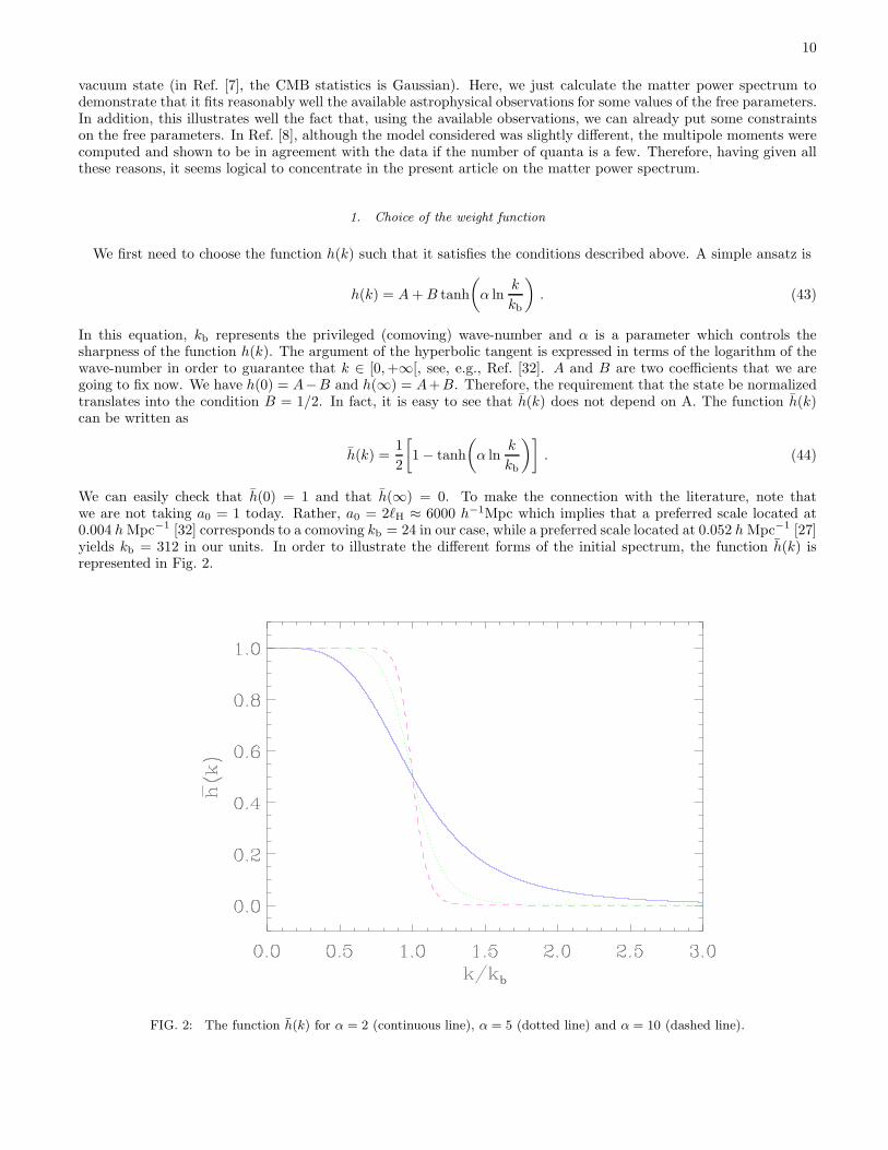
We can easily check that h(0) = 1 and that h(∞) = 0. To make the connection with the literature, note thatwe are not taking a0 = 1 today. Rather, a0 = 2ℓH ≈ 6000 h−1Mpc which implies that a preferred scale located at0.004 h Mpc−1 [32] corresponds to a comoving kb = 24 in our case, while a preferred scale located at 0.052 h Mpc−1 [27]yields kb = 312 in our units. In order to illustrate the different forms of the initial spectrum, the function h(k) isrepresented in Fig. 2.
FIG. 2: The function h(k) for α = 2 (continuous line), α = 5 (dotted line) and α = 10 (dashed line).
11
At this point, we need to re-investigate the back-reaction problem described before but now for the two non-vacuumstates |Ψ1〉 and |Ψ2〉. In particular, we are going to see that we can put some constraints on the free parameters onlyfrom theoretical considerations. An analogous analysis to the one performed in Section II, now for the state |Ψ1〉leads to
〈Ψ1|ρ|Ψ1〉 =1
8π3a4
∫ +∞
0
dk
kk2[1 + 2nδ(k ∈ D)]
[
µ′kµ′∗
k − a′
a(µkµ′∗
k + µ∗kµ′
k) +
(
a′2
a2+ k2
)
µkµ∗k
]
, (45)
〈Ψ1|p|Ψ1〉 =1
8π3a4
∫ +∞
0
dk
kk2[1 + 2nδ(k ∈ D)]
[
µ′kµ′∗
k − a′
a(µkµ′∗
k + µ∗kµ′
k) +
(
a′2
a2− k2
3
)
µkµ∗k
]
. (46)
Again, as in Section II, the term which is not proportional to n should be subtracted since it represents the vacuumcontribution. Now, for the state |Ψ2〉, one gets
〈Ψ2|ρ|Ψ2〉 =
∫ +∞
0
∫ +∞
0
dσdσ′g∗(σ)g(σ′)〈Ψ1(σ, n)|ρ|Ψ1(σ′, n)〉 (47)
=
∫ +∞
0
dσ|g(σ)|2〈Ψ1(σ, n)|ρ|Ψ1(σ, n)〉, (48)
where we used the fact that ρ does not act on σ. In the high-frequency regime, one obtains
〈Ψ2|ρ|Ψ2〉 = 〈0|ρ|0〉 +n
16π2a4
∫ ∞
0
σ4|g(σ)|2dσ, (49)
〈Ψ2|p|Ψ2〉 = 〈0|p|0〉 +1
3
n
16π2a4
∫ ∞
0
σ4|g(σ)|2dσ. (50)
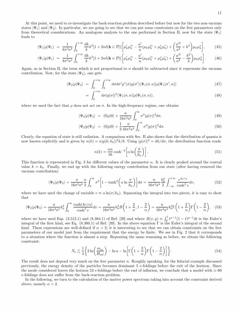
Clearly, the equation of state is still radiation. A comparison with Sec. II also shows that the distribution of quanta isnow known explicitly and is given by n(k) = n|g(k; kb)|2k/8. Using |g(σ)|2 = dh/dσ, the distribution function reads
n(k) =αn
16cosh−2
[
α ln
(
k
kb
)]
. (51)
This function is represented in Fig. 3 for different values of the parameter α. It is clearly peaked around the centralvalue k = kb. Finally, we end up with the following energy contribution from our state (after having removed thevacuum contribution)
〈Ψ2|ρ|Ψ2〉 =n
16π2a4
α
2
∫ ∞
0
σ3
[
1 − tanh2
(
α lnσ
kb
)]
dσ =n
16π2a4
k4b
2
∫ +∞
−∞
e4v/α
cosh2 vdv, (52)
where we have used the change of variable v ≡ α ln(σ/kb). Separating the integral into two pieces, it is easy to showthat
〈Ψ2|ρ|Ψ2〉 =n
16π2a4k4b
∫ ∞
0
cosh(4v/α)
cosh2 vdv =
n
16π2a4k4bB
(
1 +2
α, 1 − 2
α
)
=n
16π2a4k4bΓ
(
1 +2
α
)
Γ
(
1 − 2
α
)
, (53)
where we have used Eqs. (3.512.1) and (8.384.1) of Ref. [39] and where B(x, y) ≡∫ 1
0 tx−1(1 − t)y−1dt is the Euler’sintegral of the first kind, see Eq. (8.380.1) of Ref. [39]. In the above equation Γ is the Euler’s integral of the secondkind. These expressions are well-defined if α > 2; it is interesting to see that we can obtain constraints on the freeparameters of our model just from the requirement that the energy be finite. We see in Fig. 2 that it correspondsto a situation where the function is almost a step. Repeating the same reasoning as before, we obtain the followingconstraint:
Ne .1
4
2 ln
(
mPl
Hinf
)
− lnn − ln
[
Γ
(
1 +2
α
)
Γ
(
1 − 2
α
)]
. (54)
The result does not depend very much on the free parameter n. Roughly speaking, for the fiducial example discussedpreviously, the energy density of the particles becomes dominant 5 e-foldings before the exit of the horizon. Sincethe mode considered leaves the horizon 53 e-foldings before the end of inflation, we conclude that a model with ≃ 60e-foldings does not suffer from the back-reaction problem.
In the following, we turn to the calculation of the matter power spectrum taking into account the constraint derivedabove, namely α > 2.
12
FIG. 3: The function n(k) for kb = 312, n = 1, α = 2 (continuous line), α = 5 (dotted line) and α = 10 (dashed line).
2. Calculation of the power spectrum
The first step is to calculate the two-point correlation function of the Bardeen potential. Most of the calculation hasalready been done in the previous subsection, see Eq. (36), but what matters now is the coefficient of proportionalitywhich was not determined previously. One finds
〈Ψ2(n, kb)|Φ(η,x)Φ(η,x + r)|Ψ2(n, kb)〉 =ℓ2Pl
ℓ20
9
4π
∫ ∞
0
dk
k
sin kr
krk3|fk|2[1 + 2nh(k)]. (55)
The link between the power spectrum and the classical Fourier component of the Bardeen potential Φ(η,k), withΦ(η,x) = 1/(2π)3/2
∫
dkΦ(η,k)eik·x, is obtained if one uses an ergodic hypothesis and identifies the “quantum”two-point correlation function with the spatial average 〈Φ(η,x)Φ(η,x + r)〉V. In this case, one finds
〈Φ(η,x)Φ(η,x + r)〉V =1
2π2
∫ ∞
0
dk
k
sin kr
krk3|Φ(η,k)|2 ⇒ 1
2π2k3|Φ(η,k)|2 =
ℓ2Pl
ℓ20
9
4πA
SknS−1[1 + 2nh(k)]. (56)
Then, the matter power spectrum can be directly derived since the density contrast is linked to the Bardeen potentialby the perturbed Einstein equations. As we mentioned above, we take n
S= 1 for simplicity and get from the Poisson’s
equation
|δ(η,k)|2 =4
9
(
kphys
H0
)4
|Φ(η,k)|2 ⇒ |δ(η,k)|2 =π
4H0
ℓ2Pl
ℓ20
ASkphys[1 + 2nh(k)], (57)
where AS
is the constant fixed by the COBE normalization, see Eq. (39). The quantity δ(η,k) in the last equationsis dimensionless. The dimension-full (physical) Fourier component of the square of the density contrast is just a6
0
times the previous one, a0 being the value of the scale factor today. Defining, as usual, the spectrum P (k) byP (k) ≡ |δphys(η,k)|2/a3
0 and choosing the normalization of the scale factor as a0 = 2ℓH where ℓH is the Hubble radiustoday, one finds
P (k) =16π
5H40
Q2rms−PS
T 20
1
W22
[
1
6π+ 2nD
(2)2 (kb)
]−1[
1 + 2nh(k)
]
kphys . (58)
13
This equation gives the initial matter power spectrum. In order to obtain the matter power spectrum today, we needto take into account the transfer function T (k) which describes the evolution of the Fourier modes inside the horizon.In that case, one has
P (k) = T 2(k)16π
5H40
Q2rms−PS
T 20
1
W22
[
1
6π+ 2nD
(2)2 (kb)
]−1[
1 + 2nh(k)
]
kphys . (59)
The sCDM transfer function is given approximatively by the following numerical fit [40]
T (k) =ln(1 + 2.34q)
2.34q
[
1 + 3.89q + (16.1q)2 + (5.46q)3 + (6.71q)4]−1/4
, q ≡ k/[(hΓ)Mpc−1] , (60)
where Γ is the so-called shape parameter, which can be written as [40]
Γ ≡ Ω0he−Ωb−√
2hΩb/Ω0 , (61)
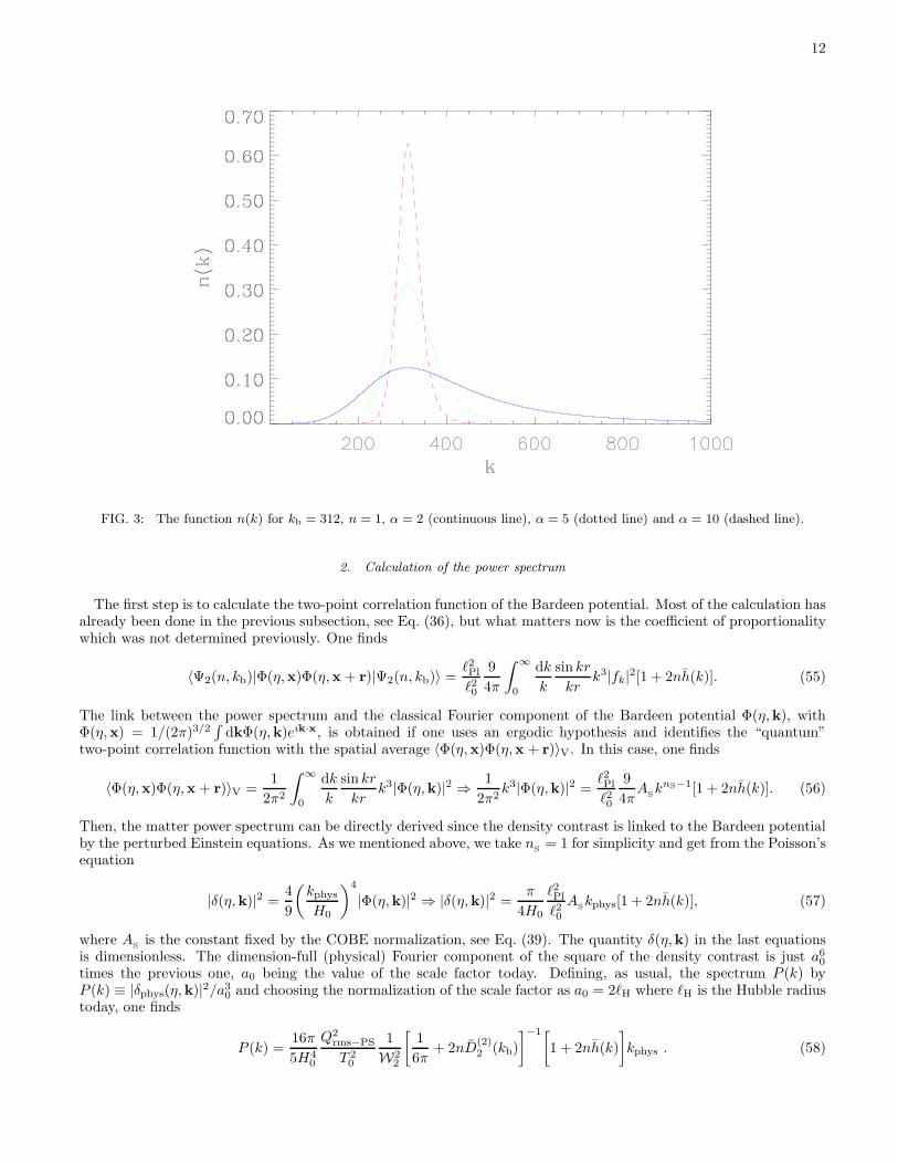
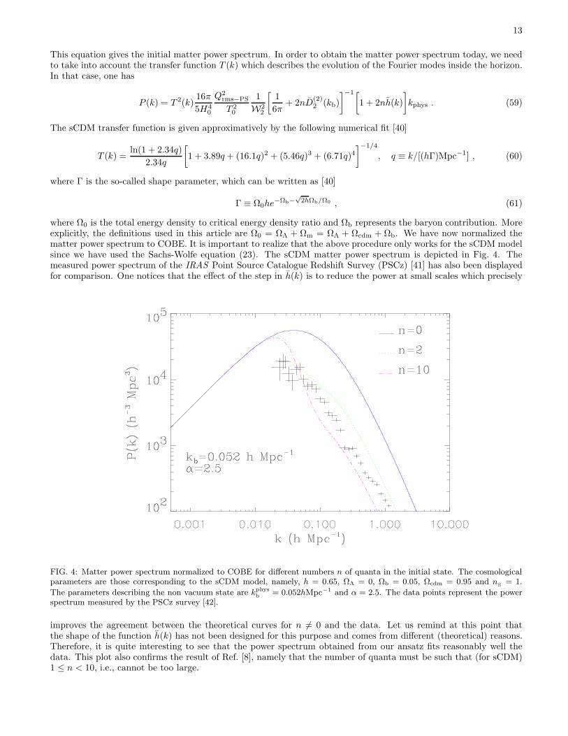
where Ω0 is the total energy density to critical energy density ratio and Ωb represents the baryon contribution. Moreexplicitly, the definitions used in this article are Ω0 = ΩΛ + Ωm = ΩΛ + Ωcdm + Ωb. We have now normalized thematter power spectrum to COBE. It is important to realize that the above procedure only works for the sCDM modelsince we have used the Sachs-Wolfe equation (23). The sCDM matter power spectrum is depicted in Fig. 4. Themeasured power spectrum of the IRAS Point Source Catalogue Redshift Survey (PSCz) [41] has also been displayedfor comparison. One notices that the effect of the step in h(k) is to reduce the power at small scales which precisely
FIG. 4: Matter power spectrum normalized to COBE for different numbers n of quanta in the initial state. The cosmologicalparameters are those corresponding to the sCDM model, namely, h = 0.65, ΩΛ = 0, Ωb = 0.05, Ωcdm = 0.95 and n
S= 1.
The parameters describing the non vacuum state are kphysb = 0.052hMpc−1 and α = 2.5. The data points represent the power
spectrum measured by the PSCz survey [42].
improves the agreement between the theoretical curves for n 6= 0 and the data. Let us remind at this point thatthe shape of the function h(k) has not been designed for this purpose and comes from different (theoretical) reasons.Therefore, it is quite interesting to see that the power spectrum obtained from our ansatz fits reasonably well thedata. This plot also confirms the result of Ref. [8], namely that the number of quanta must be such that (for sCDM)1 ≤ n < 10, i.e., cannot be too large.
14
Another more accurate test to check the consistency of the model with the observations is to compute the rms massfluctuation at a scale of r0 = 8h−1Mpc. Its definition for a top hat window function reads
σ28 ≡
(
δM
M
)2
(r0 = 8h−1Mpc) =1
(4πr30/3)2
∫ ∞
0
k3P (k)
2π2W 2(k)
dk
k, (62)
with
W (k) = 4πr30
[
sin kr0
(kr0)3− cos kr0
(kr0)2
]
. (63)
For n = 0 (i.e. standard sCDM model) with the following choice for the cosmological parameters, h = 0.65, Ω0 = 1,Ωb = 0.05, a numerical calculation of the previous integral gives σ8 ≃ 1.67, in agreement with previous estimates, seeFig. 15 of Ref. [43]. For h = 0.5, the result becomes σ8 ≃ 1.28 which is also consistent with Ref. [43]. Let us now
calculate the rms mass fluctuation for n 6= 0. For α = 2, kphysb = 0.052h Mpc−1 one finds, for our fiducial choice of
the cosmological parameters, σ8 ≃ 0.99, 0.79, 0.68 for n = 1, 2, 3 respectively. In the same conditions, but for α = 5,one obtains σ8 ≃ 0.98, 0.77, 0.66 which illustrates explicitly the fact that σ8 is not sensitive to the parameter α. Thesenumbers should now be compared with those inferred from cluster abundance constraints [44] which give
σclu8 = (0.5 ± 0.1)Ω−γ
m , (64)
where γ ≃ 0.5. We recover the well-known conclusion that the n = 0 sCDM model is ruled out because the CMB andclusters normalization are not consistent with each other (i.e. the difference is greater than 5σ). On the other hand,we see that putting a few quanta improves the situation and that the n = 2 model becomes compatible with the dataat the 3σ level whereas the model n = 3 gives the correct value at less than 2σ. Fine-tuning the other cosmologicalparameters would allows us to achieve an even better agreement. Therefore, as announced, there exists a region inthe space of parameters where the model is in agreement with the presently available data.
Now, we would like also to test the predictions of the model in the case where a cosmological constant is present. Afirst problem is that the value of the coefficient A
Sis no longer the same. The reason is that the integrated Sachs-Wolfe
effect now plays a role at large scales and modifies the relation (24). This changes the COBE normalization and we
have C(2)2 (ΩΛ 6= 0) 6= C
(2)2 (ΩΛ = 0). As a consequence, the constant A
Sin Eq. (26) is no longer given by Eq. (39) and
has to be evaluated numerically for each value of the cosmological constant. We can parameterize this dependence byintroducing a coefficient B
S(ΩΛ) such that A
S(ΩΛ 6= 0) = B
S(ΩΛ)A
S(ΩΛ = 0). Obviously, one has B
S(ΩΛ = 0) = 1.
A second problem is that the transfer function is also modified by the presence of a cosmological constant. However,the change can be easily parameterized by using a new numerical fit to the transfer function. Finally, the powerspectrum can be written as
P (k) = T 2(k)g2(Ω0)
g2(Ωm)B
S(ΩΛ)
16π
5H40
Q2rms−PS
T 20
1
W22
[
1
6π+ 2nD
(2)2 (kb)
]−1[
1 + 2nh(k)
]
kphys , (65)
where the function g(Ω) takes into account the modification induced in the transfer function by the presence of acosmological constant. Its expression can be written as [45]:
g(Ω) ≡ 5Ω
2
[
Ω4/7 − ΩΛ +
(
1 +Ω
2
)(
1 +ΩΛ
70
)]−1
. (66)
Using the previous expression, we deduce that
σ28(Ω0, Ωcdm, Ωb, ΩΛ, n) =
g2(Ω0)
g2(Ωm)B
S(ΩΛ)σ2
8(Ω0, Ωcdm, Ωb, ΩΛ = 0, n), (67)
where the last term, σ28(Ω0, Ωcdm, Ωb, ΩΛ = 0, n) does not depend explicitly on Ωcdm since this one does not appear
in the shape parameter and therefore neither in the transfer function. Therefore, this term is equal to the valuecomputed previously for the sCDM model. From this last equation one can easily deduce the constant B
S(ΩΛ), and
we finally obtain
σ28(Ω0, Ωcdm, Ωb, ΩΛ, n) =
σ28(Ω0, Ωcdm, Ωb, ΩΛ, n = 0)
σ28(Ω0, Ωcdm, Ωb, ΩΛ = 0, n = 0)
σ28(Ω0, Ωcdm, Ωb, ΩΛ = 0, n). (68)
The quantity σ28(Ω0, Ωcdm, Ωb, ΩΛ, n = 0) is known in the literature since it is nothing but the value for the ΛCDM
model. For our choice of the cosmological parameters, one has, for the ΛCDM model with ΩΛ = 0.7, σ8 ≃ 1 in
15
agreement with Fig. 16 of Ref. [43]. The quantity σ28(Ω0, Ωcdm, Ωb, ΩΛ = 0, n = 0) is the value corresponding to
sCDM. Finally, the quantity σ28(Ω0, Ωm, Ωb, ΩΛ = 0, n) is known from the previous calculations. Hence, for the values
of the parameters considered above, one finds σ8 ≃ 0.59, 0.47, 0.40 for n = 1, 2, 3 respectively. This has to be comparedwith σclu
8 which is now equal to σclu8 ≃ 0.91 [46, 47, 48]. In this case, we see that already the first value n = 1 gives a
too small contribution. This had already been noticed in Ref. [8] for the CMB anisotropy. In this case the presenceof the cosmological constant increases the height of the first acoustic peak which is also the effect of adding moreand more quanta. This can result in an acoustic peak which is too high. The cure is obvious: one has to decreasethe value of the cosmological constant as also noticed in Ref. [7]. For instance, for ΩΛ = 0.5, the value of σ8 for theΛCDM model becomes σ8 ≃ 1.25, see Fig. 16 of Ref. [43]. This gives for our model σ8 ≃ 0.74, 0.59, 0.51 for n = 1, 2, 3which goes in the right direction. The model with n = 1 is now compatible at the 1.5σ level. One can decrease morethe value of ΩΛ in order to obtain a better agreement. These numbers are in full agreement with those proposed inRef. [7] where the range for the cosmological constant in a BSI model with p > 1 was found to be 0.2 < ΩΛ < 0.5.Again, this is not surprising since we essentially deal with (almost) the same two-point correlation function.
IV. FOUR-POINT CORRELATION FUNCTION FOR NON-VACUUM INITIAL STATES
A. General expressions
In this section we proceed with the calculation of the four-point correlation function. We first perform the calculationfor the state |Ψ1〉, which we then generalize for the state |Ψ2〉. The first step is to establish the expression of all thecombinations of four creation and/or annihilation operators taken in the state |Ψ1(σ, n)〉. One finds
〈Ψ1(σ, n)|ckcpc†qc†s|Ψ1(σ, n)〉 =
[
δ(p − s)δ(k − q) + δ(p − q)δ(k − s)
]
×[
1 + nδ(s ∈ D) + nδ(q ∈ D) + n2δ(s ∈ D)δ(q ∈ D)
]
−n(n + 1)δ(s ∈ D)δ(q − s)δ(p − s)δ(k − q) , (69)
〈Ψ1(σ, n)|c†kc†pcqcs|Ψ1(σ, n)〉 = n2δ(s ∈ D)δ(q ∈ D)
[
δ(p − s)δ(k − q) + δ(p − q)δ(k − s)
]
−n(n + 1)δ(s ∈ D)δ(q − s)δ(p − s)δ(k − q) , (70)
〈Ψ1(σ, n)|c†kcpc†qcs|Ψ1(σ, n)〉 = nδ(s ∈ D)δ(p − q)δ(k − s) + n2δ(s ∈ D)δ(q ∈ D)δ(p − q)δ(k − s)
+n2δ(s ∈ D)δ(p ∈ D)δ(q − s)δ(k − p)
−n(n + 1)δ(s ∈ D)δ(q − s)δ(p − q)δ(k − s) , (71)
〈Ψ1(σ, n)|ckc†pc†qcs|Ψ1(σ, n)〉 = nδ(s ∈ D)
[
δ(q − s)δ(k − p) + δ(p − s)δ(k − q)
]
+n2δ(s ∈ D)δ(k ∈ D)
[
δ(q − s)δ(k − p) + δ(p− s)δ(k − q)
]
−n(n + 1)δ(s ∈ D)δ(q − s)δ(p − s)δ(k − q) , (72)
〈Ψ1(σ, n)|c†kcpcqc†s|Ψ1(σ, n)〉 = +nδ(k ∈ D)
[
δ(p − s)δ(k − q) + δ(q − s)δ(k − p)
]
+n2δ(s ∈ D)δ(k ∈ D)
[
δ(q − s)δ(k − p) + δ(p− s)δ(k − q)
]
−n(n + 1)δ(s ∈ D)δ(q − s)δ(p − s)δ(k − q) , (73)
〈Ψ1(σ, n)|ckc†pcqc†s|Ψ1(σ, n)〉 = δ(q − s)δ(k − p) + nδ(s ∈ D)δ(q − s)δ(k − p)
+nδ(q ∈ D)δ(p − q)δ(k − s) + nδ(p ∈ D)δ(q − s)δ(k − p)
+n2δ(s ∈ D)δ(p ∈ D)
[
δ(q − s)δ(k − p) + δ(p − q)δ(k − s)
]
−n(n + 1)δ(s ∈ D)δ(q − s)δ(p − q)δ(k − s) . (74)
16
Then we can use the previous equations to calculate the expectation value of four coefficients aℓm in the state|Ψ1(σ, n)〉. Using Eq. (28) which links the operators aℓm to the operators ck, one obtains
〈Ψ1(σ, n)|aℓ1m1aℓ2m2
aℓ3m3aℓ4m4
|Ψ1(σ, n)〉 =ℓ4Pl
ℓ40
(−1)m1+m2
[
Cℓ1Cℓ2 + 2nCℓ1D(1)ℓ2
+ 2nCℓ2D(1)ℓ1
+ 4n2D(1)ℓ1
D(1)ℓ2
]
δℓ1ℓ3δℓ2ℓ4δm1,−m3δm2,−m4
+(−1)m1+m2
[
Cℓ1Cℓ2 + 2nCℓ1D(1)ℓ2
+ 2nCℓ2D(1)ℓ1
+ 4n2D(1)ℓ1
D(1)ℓ2
]
δℓ1ℓ4δℓ2ℓ3δm1,−m4δm2,−m3
+(−1)m1+m3
[
Cℓ1Cℓ3 + 2nCℓ1D(1)ℓ3
+ 2nCℓ3D(1)ℓ1
+ 4n2D(1)ℓ1
D(1)ℓ3
]
δℓ1ℓ2δℓ3ℓ4δm1,−m2δm3,−m4
−2n(n + 1)E(1)ℓ1ℓ2ℓ3ℓ4
Hm1m2m3m4
ℓ1ℓ2ℓ3ℓ4eiπ(ℓ1+ℓ2+ℓ3+ℓ4)/2
[
(−1)ℓ1+ℓ2+ℓ3+ℓ4 + (−1)ℓ1+ℓ3 + (−1)ℓ2+ℓ3
]
, (75)
with
E(1)ℓ1ℓ2ℓ3ℓ4
≡∫ σ
0
jℓ1 [k(η0 − ηlss)]jℓ2 [k(η0 − ηlss)]jℓ3 [k(η0 − ηlss)]jℓ4 [k(η0 − ηlss)]k3|fk|4
dk
k, (76)
Hm1m2m3m4
ℓ1ℓ2ℓ3ℓ4≡
∫
dΩeY∗ℓ1m1
(−e)Y ∗ℓ2m2
(−e)Y ∗ℓ3m3
(e)Y ∗ℓ4m4
(e) . (77)
Let us notice the following technical trick. Originally, in front of the first squared bracket in Eq. (75) appears a termof the form (−1)ℓ1+ℓ2eiπ(ℓ1+ℓ2+ℓ3+ℓ4)/2. Using the fact that the presence of the Kronecker symbols implies that thecorresponding expression inside the squared bracket is non vanishing only if ℓ1 = ℓ3 and ℓ2 = ℓ4, the previous termcan be rewritten as e2iπ(ℓ1+ℓ2) = 1. This explains why it does not appear explicitly in Eq. (75). Similar manipulationscan be performed for the terms in front of the following two squared brackets. Let us also notice that Eq. (75) includesa complex exponential factor, namely exp[iπ(ℓ1 + ℓ2 + ℓ3 + ℓ4)/2]. However, by inspection of the properties of thequantity Hm1m2m3m4
ℓ1ℓ2ℓ3ℓ4, see its definition in terms of Clebsh-Gordan coefficients in the Appendix, it is possible to show
that this term is in fact real. Indeed since the Clebsh-Gordan coefficients are non-vanishing only if ℓ1 + ℓ2 + L = 2pand ℓ3 + ℓ4 +L = 2q where p, q are integers, we have ℓ1 + ℓ2 + ℓ3 + ℓ4 = 2(p+ q−L), i.e., an even number. Therefore,the complex exponential factor in Eq. (75) is real and equal to either 1 or −1. These technical considerations will beemployed in the formulas below. We also see that we now have (−1)ℓ1+ℓ2+ℓ3+ℓ4 = 1. Finally, Eq. (75) can be castinto a more compact form
〈Ψ1(σ, n)|aℓ1m1aℓ2m2
aℓ3m3aℓ4m4
|Ψ1(σ, n)〉 =ℓ4Pl
ℓ40
(−1)m1+m2C(1)ℓ1
C(1)ℓ2
δℓ1ℓ3δℓ2ℓ4δm1,−m3δm2,−m4
+(−1)m1+m2C(1)ℓ1
C(1)ℓ2
δℓ1ℓ4δℓ2ℓ3δm1,−m4δm2,−m3
+ (−1)m1+m3C(1)ℓ1
C(1)ℓ3
δℓ1ℓ2δℓ3ℓ4δm1,−m2δm3,−m4
−2n(n + 1)E(1)ℓ1ℓ2ℓ3ℓ4
Hm1m2m3m4
ℓ1ℓ2ℓ3ℓ4eiπ(ℓ1+ℓ2+ℓ3+ℓ4)/2
[
1 + (−1)ℓ1+ℓ3 + (−1)ℓ2+ℓ3
]
. (78)
The first part of this equation has the same structure as the corresponding well-known equation for the vacuum state.
It is sufficient to replace Cℓ with C(1)ℓ in the latter to obtain the first part of Eq. (78). However, in addition, there
is a non trivial term proportional to the coefficient E(1)ℓ1ℓ2ℓ3ℓ4
which cannot be guessed a priori. Obviously, for n = 0,one recovers the standard result.
The calculation of the four-point correlation function in the state |Ψ2〉 is a bit more involved. Using the fact thatthe operators aℓm do not act on σ, one finds that the general expression is given by
〈Ψ2(n, kb)|aℓ1m1aℓ2m2
aℓ3m3aℓ4m4
|Ψ2(n, kb)〉 =
∫ ∞
0
dσg2(σ; kb)〈Ψ1(σ, n)|aℓ1m1aℓ2m2
aℓ3m3aℓ4m4
|Ψ1(σ, n)〉. (79)
The integration of terms of the type Cℓ1Cℓ2 , Cℓ1D(1)ℓ2
and E(1)ℓ1ℓ2ℓ3ℓ4
is easy and proceeds as before. The most difficult
part is the integration of terms of the type D(1)ℓ1
D(1)ℓ2
. We find that, in the state |Ψ2〉, the four-point correlationfunction is given by
〈Ψ2(n, kb)|aℓ1m1aℓ2m2
aℓ3m3aℓ4m4
|Ψ2(n, kb)〉 =ℓ4Pl
ℓ40
17
(−1)m1+m2
[
Cℓ1Cℓ2 + 2nCℓ1D(2)ℓ2
+ 2nCℓ2D(2)ℓ1
+ 4n2F(2)ℓ1ℓ2
]
δℓ1ℓ3δℓ2ℓ4δm1,−m3δm2,−m4
+(−1)m1+m2
[
Cℓ1Cℓ2 + 2nCℓ1D(2)ℓ2
+ 2nCℓ2D(2)ℓ1
+ 4n2F(2)ℓ1ℓ2
]
δℓ1ℓ4δℓ2ℓ3δm1,−m4δm2,−m3
+(−1)m1+m3
[
Cℓ1Cℓ3 + 2nCℓ1D(2)ℓ3
+ 2nCℓ3D(2)ℓ1
+ 4n2F(2)ℓ1ℓ3
]
δℓ1ℓ2δℓ3ℓ4δm1,−m2δm3,−m4
−2n(n + 1)E(2)ℓ1ℓ2ℓ3ℓ4
Hm1m2m3m4
ℓ1ℓ2ℓ3ℓ4eiπ(ℓ1+ℓ2+ℓ3+ℓ4)/2
[
1 + (−1)ℓ1+ℓ3 + (−1)ℓ2+ℓ3
]
, (80)
with
F(2)ℓ1ℓ2
≡∫ +∞
0
dσh(σ)d
dσ
[
D(1)ℓ1
D(1)ℓ2
]
=π2
4A2
S
∫ +∞
0
dσh(σ)d
dσ
[
D(1)ℓ1
D(1)ℓ2
]
≡ π2
4A2
SF
(2)ℓ1ℓ2
(81)
E(2)ℓ1ℓ2ℓ3ℓ4
≡∫ +∞
0
jℓ1 [k(η0 − ηlss)]jℓ2 [k(η0 − ηlss)]jℓ3 [k(η0 − ηlss)]jℓ4 [k(η0 − ηlss)]h(k)k3|fk|4dk
k
=π2
4A2
S
∫ +∞
0
Jℓ1+1/2(k)Jℓ2+1/2(k)Jℓ3+1/2(k)Jℓ4+1/2(k)h(k)k2nS−8dk ≡ π2
4A2
SE
(2)ℓ1ℓ2ℓ3ℓ4
. (82)
We now see clearly the complication brought into the problem by the term F(2)ℓ1ℓ2
. This term prevents us to reduce
the terms within the squared brackets to the natural form C(2)ℓ1
C(2)ℓ2
because F(2)ℓ1ℓ2
6= D(2)ℓ1
D(2)ℓ2
.
B. Calculation of the excess kurtosis
We are now in a position to calculate the excess kurtosis. In the previous section, we have established the expressionof the four-point correlation functions for the operator aℓm. In order to establish an analytical formula for the CMBexcess kurtosis, one just needs to use the equation linking aℓm and δT/T and to play with the properties of thespherical harmonics. Explicitly, the excess kurtosis is defined as
K ≡ µ4 − 3µ22 , (83)
where the second moment has already been introduced and where the fourth moment, µ4, of the distribution is definedas
µ4 = 〈K〉 with K ≡[
δT
T(e)
]4
. (84)
An important shortcoming of the previous definition is that the value of K depends on the normalization. It is muchmore convenient to work with a normalized (dimensionless) quantity. Therefore, we also define the normalized excesskurtosis as
Q ≡ Kµ2
2
=µ4
µ22
− 3 , (85)
which is the one more commonly used in the literature. In what follows we work with either K or Q parameters.Thus, Eqs. (33), (80) and (83) imply
K =ℓ4Pl
ℓ40
34n2
(4π)2
∑
ℓ1ℓ2
(2ℓ1 + 1)(2ℓ2 + 1)
[
F(2)ℓ1ℓ2
− D(2)ℓ1
D(2)ℓ2
]
W2ℓ1W
2ℓ2
−2n(n + 1)∑
ℓ1m1
∑
ℓ2m2
∑
ℓ3m3
∑
ℓ4m4
E(2)ℓ1ℓ2ℓ3ℓ4
Hm1m2m3m4
ℓ1ℓ2ℓ3ℓ4eiπ(ℓ1+ℓ2+ℓ3+ℓ4)/2
[
1 + (−1)ℓ1+ℓ3 + (−1)ℓ2+ℓ3
]
×Wℓ1Wℓ2Wℓ3Wℓ4Yℓ1m1(e)Yℓ2m2
(e)Yℓ3m3(e)Yℓ4m4
(e)
. (86)
Let us first concentrate on the first term in the above equation. The terms (2ℓ1 + 1)(2ℓ2 + 1) and 1/(4π)2 originatefrom the addition theorem of spherical harmonics
∑
m
Yℓm(e)Y ∗ℓm(k) =
2ℓ + 1
4πPℓ(cos e · k) . (87)
18
The factor 3 comes from the definition of K, see Eq. (83). The fact that F(2)ℓ1ℓ2
6= D(2)ℓ1
D(2)ℓ2
prevents this first term fromvanishing. This is consistent with the previous considerations, as we have seen that in the absence of this conditionthe structure of the four-point correlation function would be similar to the one in the vacuum state, up to the term
proportional to E(2)ℓ1ℓ2ℓ3ℓ4
of course. Let us now treat in more detail the second term in Eq. (86). Using again theaddition theorem of spherical harmonics and the expression of a Legendre polynomial in terms of a spherical harmonic,Yℓ0 =
√
(2ℓ + 1)/(4π)Pℓ(cos θ), we can perform the sum over the indices mi’s and express the corresponding factorin terms of the coefficient H0000
ℓ1ℓ2ℓ3ℓ4, and therefore in terms of Clebsh-Gordan coefficients, see the Appendix.
After some lengthy but straightforward algebra, one finds that the excess kurtosis in our class of models is finallygiven by
K =ℓ4Pl
ℓ40
3n2
4π2
∑
ℓ1ℓ2
(2ℓ1 + 1)(2ℓ2 + 1)
[
F(2)ℓ1ℓ2
− D(2)ℓ1
D(2)ℓ2
]
W2ℓ1W
2ℓ2
− 1
32π3n(n + 1)
∑
ℓ1ℓ2ℓ3ℓ4
(2ℓ1 + 1)(2ℓ2 + 1)(2ℓ3 + 1)(2ℓ4 + 1)E(2)ℓ1ℓ2ℓ3ℓ4
eiπ(ℓ1+ℓ2+ℓ3+ℓ4)/2Wℓ1Wℓ2Wℓ3Wℓ4
×[
1 + (−1)ℓ1+ℓ3 + (−1)ℓ2+ℓ3
] L=min(ℓ1+ℓ2,ℓ3+ℓ4)∑
L=max(|ℓ1−ℓ2|,|ℓ3−ℓ4|)(2L + 1)
(
ℓ1 ℓ2 L0 0 0
)2 (
ℓ3 ℓ4 L0 0 0
)2
. (88)
Let us emphasize that Eq. (88) is the general expression for the excess kurtosis for any non-vacuum state, since theonly information we have used about the function h(k) is that it is always positive, it vanishes at infinity, and it isa monotonically decreasing function of k. This expression is just a pure number, and it is our main result. In thefollowing, as we did in previous sections, we will choose an adequate ansatz for h(k), namely that one from Eq. (43),and compute the excess kurtosis K, as well as the normalized excess kurtosis Q defined by Eq. (85). We will thencompare the calculated value for Q to the one quantified by the cosmic variance.
In an analogous way as for the definition of the second moment µ2 given in Eq. (42), and for future convenience,we can express the excess kurtosis in terms of its “multipole moments” Kℓ1ℓ2ℓ3ℓ4 , as
K =∑
ℓ1ℓ2ℓ3ℓ4
Wℓ1Wℓ2Wℓ3Wℓ4Kℓ1ℓ2ℓ3ℓ4 . (89)
Then, from Eqs. (34), (81) and (82), it is easy to establish that the moments Kℓ1ℓ2ℓ3ℓ4 can be put under the form
Kℓ1ℓ2ℓ3ℓ4 =ℓ4Pl
ℓ40
A2S
3n2
16(2ℓ1 + 1)(2ℓ2 + 1)
[
F(2)ℓ1ℓ2
− D(2)ℓ1
D(2)ℓ2
]
δℓ1ℓ3δℓ2ℓ4
− 1
128πn(n + 1)(2ℓ1 + 1)(2ℓ2 + 1)(2ℓ3 + 1)(2ℓ4 + 1)E
(2)ℓ1ℓ2ℓ3ℓ4
(−1)(ℓ1+ℓ2+ℓ3+ℓ4)/2
×[
1 + (−1)ℓ1+ℓ3 + (−1)ℓ2+ℓ3
] L=min(ℓ1+ℓ2,ℓ3+ℓ4)∑
L=max(|ℓ1−ℓ2|,|ℓ3−ℓ4|)(2L + 1)
(
ℓ1 ℓ2 L0 0 0
)2 (
ℓ3 ℓ4 L0 0 0
)2
. (90)
The last step consists in normalizing the spectrum. For that, we use the value of AS
determined previously (in thesCDM case with non-vanishing quanta n in the vacuum state). We obtain
Kℓ1ℓ2ℓ3ℓ4 =Q4
rms−PS
T 40
64
25
1
W42
1
23−ns
Γ(3 − ns)Γ[2 + (ns − 1)/2]
Γ2[(4 − ns)/2]Γ[4 − (ns − 1)/2]+ 2nD
(2)2
−2
×
3n2
16(2ℓ1 + 1)(2ℓ2 + 1)
[
F(2)ℓ1ℓ2
− D(2)ℓ1
D(2)ℓ2
]
δℓ1ℓ3δℓ2ℓ4 −1
128πn(n + 1)(2ℓ1 + 1)(2ℓ2 + 1)
×(2ℓ3 + 1)(2ℓ4 + 1)E(2)ℓ1ℓ2ℓ3ℓ4
(−1)(ℓ1+ℓ2+ℓ3+ℓ4)/2
[
1 + (−1)ℓ1+ℓ3 + (−1)ℓ2+ℓ3
]
×L=min(ℓ1+ℓ2,ℓ3+ℓ4)
∑
L=max(|ℓ1−ℓ2|,|ℓ3−ℓ4|)(2L + 1)
(
ℓ1 ℓ2 L0 0 0
)2 (
ℓ3 ℓ4 L0 0 0
)2
. (91)
In particular, we have the following expression for Kℓℓℓℓ:
Kℓℓℓℓ =Q4
rms−PS
T 40
64
25
1
W42
1
23−ns
Γ(3 − ns)Γ[2 + (ns − 1)/2]
Γ2[(4 − ns)/2]Γ[4 − (ns − 1)/2]+ 2nD
(2)2
−2
19
×
3n2
16(2ℓ + 1)2
[
F(2)ℓℓ − D
(2)ℓ D
(2)ℓ
]
− 3
128πn(n + 1)(2ℓ + 1)4E
(2)ℓℓℓℓ
L=2ℓ∑
L=0
(2L + 1)
(
ℓ ℓ L0 0 0
)4
. (92)
This expression for the multipole moments will be employed in the next section to estimate the overall amplitude ofthe non-Gaussian signal from non-vacuum states in a semi-analytical manner.
Let us end this section by signaling that the explicit expression for the normalized excess kurtosis parameter can beeasily derived from the above formulas. Then, since this derivation is not especially illuminating, we prefer to jumpdirectly to the numerical evaluation.
V. RESULTS
Having established the formal expression of the excess kurtosis, we now turn to the question of its numericalevaluation. As we are going to see, it turns out that it is not possible to calculate everything analytically for ourspecific ansatz. Therefore, we start with giving a detailed order-of-magnitude estimate of the excess kurtosis employingthe model described above. After this, in the second subsection, we present a full numerical evaluation of Q. Theanalytical estimate will help us in roughly understanding the full numerical results. Finally, a comparison with thecosmic variance of the excess kurtosis will tell us about the feasibility of detecting this non-Gaussian signal. Readersinterested in just the final result can skip this first subsection and continue reading in section V.B.
A. Approximate analysis
In what follows, we estimate the order of magnitude of the expected excess kurtosis. We first study the function
D(1)ℓ (σ), defined in Section III as
D(1)ℓ (σ) ≡
∫ σ
0
J2ℓ+1/2(k)knS−3dk . (93)
The plot of this function is represented in Fig. 5. We can easily understand the qualitative behavior of this function.For small values of the argument, we take the first term of the Taylor expansion of the Bessel function and performthe integration exactly. The result reads
D(1)ℓ (σ) ≃ 1
22ℓ+1(2ℓ + nS − 1)Γ2(ℓ + 3/2)σ2ℓ+nS−1, σ ≪ 1 . (94)
On the other hand, for large values of the argument, using Eq. (6.574.2) of Ref. [39], we obtain
D(1)ℓ (σ) ≃ Γ[3 − nS]Γ[ℓ + (nS − 1)/2]
23−nSΓ2[2 − nS/2]Γ[ℓ + (5 − nS)/2], σ ≫ 1 . (95)
For nS = 1, the above amounts to D(1)ℓ (σ) ≃ 1/[πℓ(ℓ + 1)] which, for ℓ = 2, gives D
(1)2 (σ) ≃ 1/(6π) ≃ 0.053 in
agreement with Fig. 5. As a next step we want to understand the qualitative behavior of D(2)ℓ as a function of kb and
ℓ. Its definition, given in Section III, reads
D(2)ℓ ≡
∫ +∞
0
J2ℓ+1/2(k)h(k)knS−3dk ≃
∫ kb
0
J2ℓ+1/2(k)knS−3dk = D
(1)ℓ (kb), (96)
where we have used the fact that the behavior of h(k), especially for large value of the parameter α, is very similarto a Heaviside function. In practice, for large kb and for the range of angular frequencies we are interested in, we will
have kb ≫ ℓ. In this case, D(2)ℓ ≃ 1/[πℓ(ℓ + 1)]. Let us now try to evaluate F
(2)ℓ1ℓ2
defined by
F(2)ℓ1ℓ2
≡∫ +∞
0
dσh(σ)d
dσ
[
D(1)ℓ1
D(1)ℓ2
]
. (97)
Using again the fact that h(k) behaves like a step function, we find
F(2)ℓ1ℓ2
≃∫ kb
0
dσd
dσ
[
D(1)ℓ1
D(1)ℓ2
]
= D(1)ℓ1
(kb)D(1)ℓ2
(kb). (98)
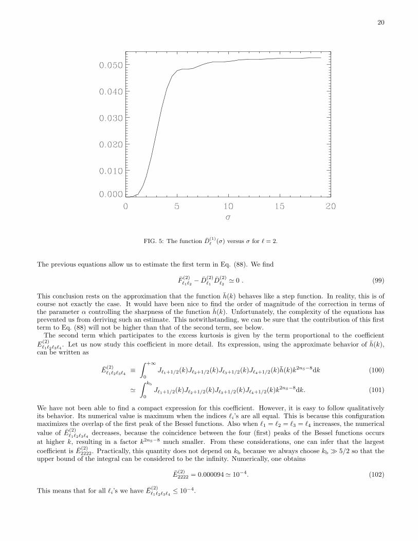
20
FIG. 5: The function D(1)ℓ
(σ) versus σ for ℓ = 2.
The previous equations allow us to estimate the first term in Eq. (88). We find
F(2)ℓ1ℓ2
− D(2)ℓ1
D(2)ℓ2
≃ 0 . (99)
This conclusion rests on the approximation that the function h(k) behaves like a step function. In reality, this is ofcourse not exactly the case. It would have been nice to find the order of magnitude of the correction in terms ofthe parameter α controlling the sharpness of the function h(k). Unfortunately, the complexity of the equations hasprevented us from deriving such an estimate. This notwithstanding, we can be sure that the contribution of this firstterm to Eq. (88) will not be higher than that of the second term, see below.
The second term which participates to the excess kurtosis is given by the term proportional to the coefficient
E(2)ℓ1ℓ2ℓ3ℓ4
. Let us now study this coefficient in more detail. Its expression, using the approximate behavior of h(k),can be written as
E(2)ℓ1ℓ2ℓ3ℓ4
≡∫ +∞
0
Jℓ1+1/2(k)Jℓ2+1/2(k)Jℓ3+1/2(k)Jℓ4+1/2(k)h(k)k2nS−8dk (100)
≃∫ kb
0
Jℓ1+1/2(k)Jℓ2+1/2(k)Jℓ3+1/2(k)Jℓ4+1/2(k)k2nS−8dk. (101)
We have not been able to find a compact expression for this coefficient. However, it is easy to follow qualitativelyits behavior. Its numerical value is maximum when the indices ℓi’s are all equal. This is because this configurationmaximizes the overlap of the first peak of the Bessel functions. Also when ℓ1 = ℓ2 = ℓ3 = ℓ4 increases, the numerical
value of E(2)ℓ1ℓ2ℓ3ℓ4
decreases, because the coincidence between the four (first) peaks of the Bessel functions occurs
at higher k, resulting in a factor k2nS−8 much smaller. From these considerations, one can infer that the largest
coefficient is E(2)2222. Practically, this quantity does not depend on kb because we always choose kb ≫ 5/2 so that the
upper bound of the integral can be considered to be the infinity. Numerically, one obtains
E(2)2222 = 0.000094 ≃ 10−4. (102)
This means that for all ℓi’s we have E(2)ℓ1ℓ2ℓ3ℓ4
≤ 10−4.
21
These semi-analytical considerations allow us to derive a rough estimate of the excess kurtosis. In the context ofour approximation, this one does not depend on kb. Let us first write Eq. (88) as follows:
K =ℓ4Pl
ℓ40
A2S(K1 + K2) (103)
and consider the first term. One has, as already mentioned previously,
K1 ≡ 3n2
16
∑
ℓ1ℓ2ℓ3ℓ4
(2ℓ1 + 1)(2ℓ2 + 1)
[
F(2)ℓ1ℓ2
− D(2)ℓ1
D(2)ℓ2
]
δℓ1ℓ3δℓ2ℓ4Wℓ1Wℓ2Wℓ3Wℓ4 ≃ 0 . (104)
Let us now study the second term. Since we have shown that the contribution of E(2)2222 dominates the sum, we can
very roughly estimate the excess kurtosis by retaining only this term. We have
K2 ≡ − 1
128πn(n + 1)
∑
ℓ1ℓ2ℓ3ℓ4
Wℓ1Wℓ2Wℓ3Wℓ4(2ℓ1 + 1)(2ℓ2 + 1)(2ℓ3 + 1)(2ℓ4 + 1)E(2)ℓ1ℓ2ℓ3ℓ4
(−1)(ℓ1+ℓ2+ℓ3+ℓ4)/2
×[
1 + (−1)ℓ1+ℓ3 + (−1)ℓ2+ℓ3
] L=min(ℓ1+ℓ2,ℓ3+ℓ4)∑
L=max(|ℓ1−ℓ2|,|ℓ3−ℓ4|)(2L + 1)
(
ℓ1 ℓ2 L0 0 0
)2 (
ℓ3 ℓ4 L0 0 0
)2
(105)
≃ −3 × 625
128πn(n + 1)E
(2)2222
L=4∑
L=0
(2L + 1)
(
2 2 L0 0 0
)4
, (106)
where we have used the fact that W2 ≃ 1 for the COBE window function, see below. The sum of the Clebsh-Gordancoefficients can easily be computed by noticing that
(
2 2 00 0 0
)
=1√5,
(
2 2 20 0 0
)
= −(
2 2 40 0 0
)
= −√
2
35, (107)
the other coefficients being zero. The numerical value of the sum is 0.0857 and we therefore reach the following result
K2 ≃ −3n(n + 1)625
128π× 0.0857× 10−4. (108)
Now, to have an order of magnitude of the contribution to the kurtosis from the second term, K2, what remains tobe done is to take into account the normalization. Using the expression of A
Sderived previously into Eq. (103) we
finally find
K ≃ −10−2πn(n + 1)
(2n + 1)2× Q4
rms−PS
T 40
. (109)
Let us again stress that there is a non-trivial guess in this calculation that can only be justified by the full numericalcalculation. The contribution of K2 is small, K2 ≪ 1. Since we have taken K1 ≃ 0, this means that, in fact, wehave assumed K2 ≫ K1. This has clearly be done without a proof because we were not able to derive an order ofmagnitude of K1 as a function of the sharpness parameter α. Nevertheless, we will see that the previous estimate isquite good.
It is also very convenient to work with the normalization-independent quantity Q. Recalling that with our approx-imations we have the second moment
µ22 ≃ 36
25
Q4rms−PS
T 40
[ℓmax∑
ℓ=2
2ℓ + 1
ℓ(ℓ + 1)W2
ℓ
]2
, (110)
it is easy to show that Q (≡ Q1 + Q2 ≃ Q2) can be written as
Q ≃ −0.0017n(n + 1)
(2n + 1)2. (111)
In the above equation we have used the COBE-DMR window function Wℓ ≃ exp[
− 12ℓ(ℓ + 1)(3.2)2
]
, where 3.2 is thedispersion of the antenna-beam profile measuring the angular response of the detector and we have chosen ℓmax = 20;
22
we find that the sum in the expression for µ22 is equal to ≃ 3.73. As an example let us take n = 2. Then we find
Q ≃ −4.09 × 10⁻⁴. Of course this number should be considered only as an order-of-magnitude estimate. It can beeasily improved if we add more terms in the calculation of the sum in the term K2. At this point, one should makeclear that taking into account more terms does not mean that we consider the next-to-leading order of a consistentexpansion. In the present context there is no small parameter to expand in. Therefore, the choice of the extra termsthat we include in the sum is a bit arbitrary. However, this is not a serious problem since we know that the term
E(2)ℓ1ℓ2ℓ3ℓ4
gives a contribution greater than the contribution coming from E(2)ℓ′1ℓ′2ℓ′3ℓ′4
provided that ℓi ≪ ℓ′i, i = 1 · · · 4.
In other words there is no mean to give a precise rule with regards to the terms that should be kept or not kept butthere is clearly a general tendency which renders the improvement of the approximation possible (otherwise the sumwould not be convergent). A good strategy to calculate the successive corrections is to proceed as follows. Supposethat we would like to calculate the sum K2 up to ℓmax. A consistent requirement is that one should take into account
all the terms E(2)ℓ1ℓ2ℓ2ℓ4
such that ℓi ≤ ℓmax, i = 1, · · · 4. For example if ℓmax = 2, then one should only include E(2)2222 as
we did in our “leading order” calculation. The next step is to consider the case ℓmax = 3, i.e., we choose to take into
account the terms E(2)2233, E
(2)3333, E
(2)2333 and E
(2)2223 (of course we should also include the terms obtained by permutations
of the indices ℓi). In fact, it is easy to see that the last two terms do not give an extra contribution because the sum∑
i ℓi is not even. For the two other terms, we find E(2)2233 ≃ 0.000041 and E
(2)3333 ≃ 0.000021. After a lengthy but
straightforward calculation, one can show that this gives an additional contribution equal to −8.51×10⁻⁶. Therefore,a more accurate estimate of the normalized excess kurtosis is
Q ≃ −4.17 × 10⁻⁴ . (112)
We now turn to a full numerical computation of this quantity.
B. Full numerical results
In the previous section we have developed a rough idea of the amplitude of Q. This gives us an estimate of theexcess kurtosis parameter. However, due to the various approximations, a full numerical resolution of Eq. (85) provesessential.
By resorting to Eq. (89) and using again the COBE-DMR window function, we can compute the value of Q, validon large angular scales. We plot the results in Fig. 6, where we show the normalized excess kurtosis Q for someparticular values of the free parameters. As we see from it, Q ≃ −4.24 × 10⁻⁴ is an asymptotic value, providedwe concentrate on the middle and big values of the built-in scale kb. This value almost exactly corresponds to thenumerical estimate derived previously. In other words, the fact that the numerical estimate does not depend on kb isconfirmed by the plot, except for small values of the wave-numbers. In fact, this shows that the quantity Q does notdepend very much on the free parameters. We have already established this property for α but this is also true for nsince, using the analytical estimate, we find, for n = 1, Q ≃ −3.77 × 10⁻⁴ and for n → ∞, Q ≃ −4.25 × 10⁻⁴. Sincewe know that this result does not depend on the details of the weight function h(k), we conclude that the asymptoticvalue obtained above is a generic value, at least for large values of kb. In particular, this is true for kb ≈ 300 whichcorresponds to the built-in scale located roughly at the privileged scale in the matter power spectrum selected by theredshift surveys of Ref. [27]. Another important remark is that the excess kurtosis is found to be negative.
Let us now try to understand qualitatively the shape of the plot Q vs. kb. The state that we consider, |Ψ2〉, is aquantum superposition of states |Ψ1〉, each one of these containing nk quanta for all the scales k up to a given, fixedscale σ [cf. Eq. (17)]. The “weight” given to each state |Ψ1〉 is described by the function g(k; kb) that depends on theprivileged scale kb. As already mentioned, for our ansatz of Eq. (43) we have g(k; kb) = (α/2k)1/2 cosh−1[α ln(k/kb)],which, as a function of k, is roughly “peaked” at kb. Then, in effect, we may approximately write
|Ψ2(n, kb)〉 ≃ |Ψ1(n, kb)〉 =⊗
k∈D(kb)
|nk〉⊗
p6∈D(kb)
|0p〉. (113)
Thus, we see that a small kb will reduce the range of scales k included in the domain D(kb), and therefore also reducethe effective available number of quanta (of energy k). Given that we employed the Sachs–Wolfe formula, the excesskurtosis that we computed is only the “trace” of the non-Gaussian signal characterized by kb left at large scales [thisis also why there is no contradiction in using Eq. (24) while kb can be large]. Let us consider two scales, say, kb1 andkb2 such that kb2 > kb1 ≫ 1 (recall that we are taking η0 − ηlss = 1). It is clear that passing from kb1 to kb2 will notchange the structure of the state |Ψ2〉 at small scales. It will just enlarge the domain where there are quanta, leavingunmodified the large scale part. Therefore, as the excess kurtosis is essentially given by the large scale part of |Ψ2〉, itmust be independent of kb provided that kb is large, exactly as we find. On the other hand, if kb is small, a change in
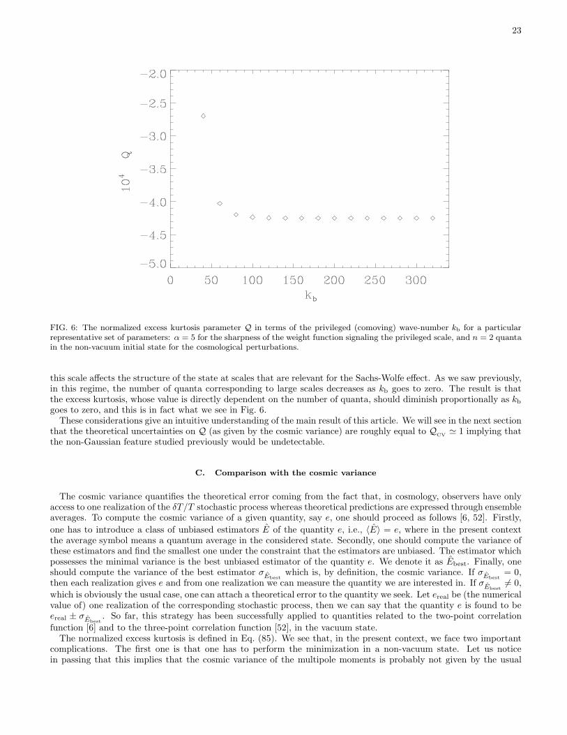
23
FIG. 6: The normalized excess kurtosis parameter Q in terms of the privileged (comoving) wave-number kb for a particularrepresentative set of parameters: α = 5 for the sharpness of the weight function signaling the privileged scale, and n = 2 quantain the non-vacuum initial state for the cosmological perturbations.
this scale affects the structure of the state at scales that are relevant for the Sachs-Wolfe effect. As we saw previously,in this regime, the number of quanta corresponding to large scales decreases as kb goes to zero. The result is thatthe excess kurtosis, whose value is directly dependent on the number of quanta, should diminish proportionally as kb
goes to zero, and this is in fact what we see in Fig. 6.These considerations give an intuitive understanding of the main result of this article. We will see in the next section
that the theoretical uncertainties on Q (as given by the cosmic variance) are roughly equal to QCV
≃ 1 implying thatthe non-Gaussian feature studied previously would be undetectable.
C. Comparison with the cosmic variance
The cosmic variance quantifies the theoretical error coming from the fact that, in cosmology, observers have onlyaccess to one realization of the δT/T stochastic process whereas theoretical predictions are expressed through ensembleaverages. To compute the cosmic variance of a given quantity, say e, one should proceed as follows [6, 52]. Firstly,
one has to introduce a class of unbiased estimators E of the quantity e, i.e., 〈E〉 = e, where in the present contextthe average symbol means a quantum average in the considered state. Secondly, one should compute the variance ofthese estimators and find the smallest one under the constraint that the estimators are unbiased. The estimator whichpossesses the minimal variance is the best unbiased estimator of the quantity e. We denote it as Ebest. Finally, oneshould compute the variance of the best estimator σEbest
which is, by definition, the cosmic variance. If σEbest= 0,
then each realization gives e and from one realization we can measure the quantity we are interested in. If σEbest6= 0,
which is obviously the usual case, one can attach a theoretical error to the quantity we seek. Let ereal be (the numericalvalue of) one realization of the corresponding stochastic process, then we can say that the quantity e is found to beereal ± σEbest
. So far, this strategy has been successfully applied to quantities related to the two-point correlation
function [6] and to the three-point correlation function [52], in the vacuum state.The normalized excess kurtosis is defined in Eq. (85). We see that, in the present context, we face two important
complications. The first one is that one has to perform the minimization in a non-vacuum state. Let us noticein passing that this implies that the cosmic variance of the multipole moments is probably not given by the usual
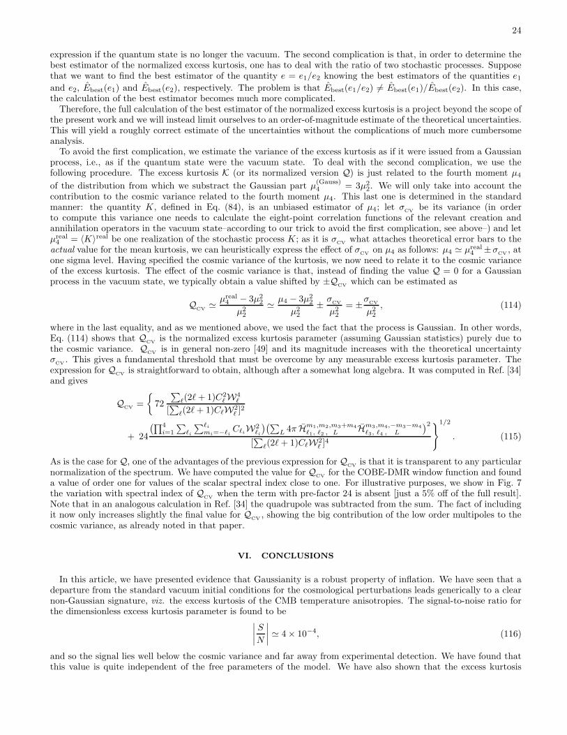
24
expression if the quantum state is no longer the vacuum. The second complication is that, in order to determine thebest estimator of the normalized excess kurtosis, one has to deal with the ratio of two stochastic processes. Supposethat we want to find the best estimator of the quantity e = e1/e2 knowing the best estimators of the quantities e1
and e2, Ebest(e1) and Ebest(e2), respectively. The problem is that Ebest(e1/e2) 6= Ebest(e1)/Ebest(e2). In this case,the calculation of the best estimator becomes much more complicated.
Therefore, the full calculation of the best estimator of the normalized excess kurtosis is a project beyond the scope ofthe present work and we will instead limit ourselves to an order-of-magnitude estimate of the theoretical uncertainties.This will yield a roughly correct estimate of the uncertainties without the complications of much more cumbersomeanalysis.
To avoid the first complication, we estimate the variance of the excess kurtosis as if it were issued from a Gaussianprocess, i.e., as if the quantum state were the vacuum state. To deal with the second complication, we use thefollowing procedure. The excess kurtosis K (or its normalized version Q) is just related to the fourth moment µ4
of the distribution from which we substract the Gaussian part µ(Gauss)4 = 3µ2
2. We will only take into account thecontribution to the cosmic variance related to the fourth moment µ4. This last one is determined in the standardmanner: the quantity K, defined in Eq. (84), is an unbiased estimator of µ4; let σ
CVbe its variance (in order
to compute this variance one needs to calculate the eight-point correlation functions of the relevant creation andannihilation operators in the vacuum state–according to our trick to avoid the first complication, see above–) and letµreal
4 = 〈K〉real be one realization of the stochastic process K; as it is σCV
what attaches theoretical error bars to theactual value for the mean kurtosis, we can heuristically express the effect of σ
CVon µ4 as follows: µ4 ≃ µreal
4 ±σCV
, atone sigma level. Having specified the cosmic variance of the kurtosis, we now need to relate it to the cosmic varianceof the excess kurtosis. The effect of the cosmic variance is that, instead of finding the value Q = 0 for a Gaussianprocess in the vacuum state, we typically obtain a value shifted by ±Q
CVwhich can be estimated as
QCV
≃ µreal4 − 3µ2
2
µ22
≃ µ4 − 3µ22
µ22
± σCV
µ22
= ±σCV
µ22
, (114)
where in the last equality, and as we mentioned above, we used the fact that the process is Gaussian. In other words,Eq. (114) shows that Q
CVis the normalized excess kurtosis parameter (assuming Gaussian statistics) purely due to
the cosmic variance. QCV
is in general non-zero [49] and its magnitude increases with the theoretical uncertaintyσ
CV. This gives a fundamental threshold that must be overcome by any measurable excess kurtosis parameter. The
expression for QCV
is straightforward to obtain, although after a somewhat long algebra. It was computed in Ref. [34]and gives
QCV
=
72
∑
ℓ(2ℓ + 1)C2ℓ W4
ℓ
[∑
ℓ(2ℓ + 1)CℓW2ℓ ]2
+ 24
(∏4
i=1
∑
ℓi
∑ℓi
mi=−ℓiCℓi
W2ℓi
)(∑
L 4π Hm1,m2,m3+m4
ℓ1, ℓ2 , L Hm3,m4,−m3−m4
ℓ3, ℓ4 , L
)2
[∑
ℓ(2ℓ + 1)CℓW2ℓ ]4
1/2
. (115)
As is the case for Q, one of the advantages of the previous expression for QCV
is that it is transparent to any particularnormalization of the spectrum. We have computed the value for Q
CVfor the COBE-DMR window function and found
a value of order one for values of the scalar spectral index close to one. For illustrative purposes, we show in Fig. 7the variation with spectral index of Q
CVwhen the term with pre-factor 24 is absent [just a 5% off of the full result].
Note that in an analogous calculation in Ref. [34] the quadrupole was subtracted from the sum. The fact of includingit now only increases slightly the final value for Q
CV, showing the big contribution of the low order multipoles to the
cosmic variance, as already noted in that paper.
VI. CONCLUSIONS
In this article, we have presented evidence that Gaussianity is a robust property of inflation. We have seen that adeparture from the standard vacuum initial conditions for the cosmological perturbations leads generically to a clearnon-Gaussian signature, viz. the excess kurtosis of the CMB temperature anisotropies. The signal-to-noise ratio forthe dimensionless excess kurtosis parameter is found to be
∣
∣
∣
∣
S
N
∣
∣
∣
∣
≃ 4 × 10⁻⁴, (116)
and so the signal lies well below the cosmic variance and far away from experimental detection. We have found thatthis value is quite independent of the free parameters of the model. We have also shown that the excess kurtosis
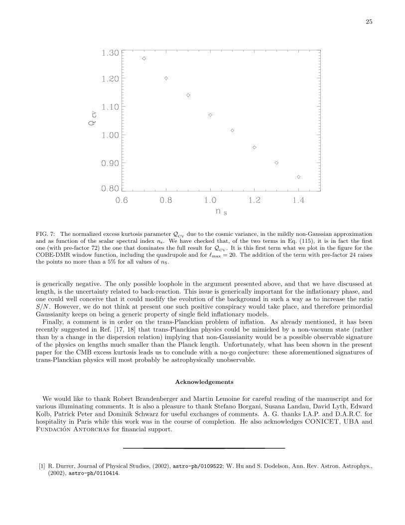
25
FIG. 7: The normalized excess kurtosis parameter QCV
due to the cosmic variance, in the mildly non-Gaussian approximationand as function of the scalar spectral index ns. We have checked that, of the two terms in Eq. (115), it is in fact the firstone (with pre-factor 72) the one that dominates the full result for Q
CV. It is this first term what we plot in the figure for the
COBE-DMR window function, including the quadrupole and for ℓmax = 20. The addition of the term with pre-factor 24 raisesthe points no more than a 5% for all values of nS.
is generically negative. The only possible loophole in the argument presented above, and that we have discussed atlength, is the uncertainty related to back-reaction. This issue is generically important for the inflationary phase, andone could well conceive that it could modify the evolution of the background in such a way as to increase the ratioS/N . However, we do not think at present one such positive conspiracy would take place, and therefore primordialGaussianity keeps on being a generic property of single field inflationary models.
Finally, a comment is in order on the trans-Planckian problem of inflation. As already mentioned, it has beenrecently suggested in Ref. [17, 18] that trans-Planckian physics could be mimicked by a non-vacuum state (ratherthan by a change in the dispersion relation) implying that non-Gaussianity would be a possible observable signatureof the physics on lengths much smaller than the Planck length. Unfortunately, what has been shown in the presentpaper for the CMB excess kurtosis leads us to conclude with a no-go conjecture: these aforementioned signatures oftrans-Planckian physics will most probably be astrophysically unobservable.
Acknowledgements
We would like to thank Robert Brandenberger and Martin Lemoine for careful reading of the manuscript and forvarious illuminating comments. It is also a pleasure to thank Stefano Borgani, Susana Landau, David Lyth, EdwardKolb, Patrick Peter and Dominik Schwarz for useful exchanges of comments. A. G. thanks I.A.P. and D.A.R.C. forhospitality in Paris while this work was in the course of completion. He also acknowledges CONICET, UBA andFundacion Antorchas for financial support.
[1] R. Durrer, Journal of Physical Studies, (2002), astro-ph/0109522; W. Hu and S. Dodelson, Ann. Rev. Astron. Astrophys.,(2002), astro-ph/0110414.
26
[2] See, e.g., http://map.gsfc.nasa.gov/ and http://astro.estec.esa.nl/Planck/ .[3] J. H. P. Wu et al., Phys. Rev. Lett. 87, 251303 (2001), astro-ph/0104248; E. Komatsu et al., submitted to Astrophys. J.,
astro-ph/0107605 ; M. G. Santos et al., astro-ph/0107588.[4] M. Kunz et al. to be published in Astrophys. J. Lett., astro-ph/0111250.[5] G. Polenta et al., astro-ph/0201133.[6] L. P. Grishchuk and J. Martin, Phys. Rev. D56, 1924 (1997), gr-qc/9702018.[7] J. Lesgourgues, D. Polarski, A. A. Starobinsky, Nucl. Phys. B 497, 479 (1997), astro-ph/9711139.[8] J. Martin, A. Riazuelo and M. Sakellariadou, Phys. Rev. D 61, 083518 (2000), astro-ph/9904167.[9] D. Boyanovsky, F. J. Cao, H. J. de Vega, astro-ph/0102474.
[10] C. R. Contaldi, R. Bean and J. Magueijo, Phys. Lett. B468, 189 (1999), astro-ph/9910309.[11] A. Linde and V. Mukhanov, Phys. Rev. D56, 535 (1997), astro-ph/9610219.[12] N. Bartolo, S. Matarrese and A. Riotto, astro-ph/0112261.[13] A. R. Liddle, D. H. Lyth, Phys. Reports 231, 1 (1993), astro-ph/9303019.[14] L. R. W. Abramo, R. H. Brandenberger and V. Mukhanov, Phys. Rev. D56, 3248 (1997), gr-qc/9704037; V. Mukhanov,
L. R. W. Abramo and R. H. Brandenberger, Phys. Rev. Lett. 78, 1624 (1997), gr-qc/9609026.[15] W. Unruh, astro-ph/9802323.[16] J. Martin and R. H. Brandenberger, Phys. Rev. D63, 123501 (2000), hep-th/0005209; R. H. Brandenberger and J. Martin,
Mod. Phys. Lett. A16, 999 (2001), astro-ph/0005432; J. Niemeyer, Phys. Rev. D63, 123502 (2000), astro-th/0005533;M. Lemoine, M. Lubo, J. Martin and J. P. Uzan, Phys. Rev. D64, 043508 (2001), hep-th/0109128; R. H. Brandenberger,S. E. Joras and J. Martin, hep-th/0112122.
[17] R. Easther, B. R. Greene, W. H. Kinney and G. Shiu, Phys. Rev. D64, 103502 (2001), hep-th/0011241; R. Easther,B. R. Greene, W. H. Kinney and G. Shiu, hep-th/0110226.
[18] L. Hui and W. H. Kinney, astro-ph/0109107.[19] P. G. Ferreira, J. Magueijo and J. Silk, Phys. Rev. D56, 4592 (1997), astro-ph/9704261.[20] P. G. Ferreira, J. Magueijo, and K. M. Gorski, Astrophys. J. 503, L1 (1998), astro-ph/9803256; A. F. Heavens,
Mon. Not. R. Astron. Soc. 299, 805 (1998), astro-ph/9804222; D. Spergel and D. Goldberg, Phys. Rev. D 59, 103001(1999), astro-ph/9811252; D. Goldberg and D. Spergel, Phys.Rev. D 59, 103002 (1999), astro-ph/9811251; L. Verde,L. Wang, A. Heavens and M. Kamionkowski, Mon. Not. R. Astron. Soc. 313, L141 (2000), astro-ph/9906301; A. Coorayand W. Hu, Astrophys. J. 534, 533 (2000), astro-ph/9910397; A. Gangui and J. Martin, Mon. Not. R. Astron. Soc. 313,323 (2000), astro-ph/9908009; A. Gangui and J. Martin, Phys. Rev. D62, 103004 (2000), astro-ph/0001361; E. Komatsuand D. Spergel, Phys. Rev. D63, 063002 (2001), astro-ph/0005036; A. Gangui, L. Pogosian, and S. Winitzki, Phys. Rev.D64, 043001 (2001), astro-ph/0101453.
[21] O. Forni and N. Aghanim, astro-ph/9905125.[22] N. Aghanim and O. Forni, astro-ph/9905124.[23] P. de Bernardis et al., Nature 404, 955 (2000), astro-ph/0004404.[24] S. Hanany et al., Astrophys. J. 545, L5 (2000), astro-ph/0005123.[25] C. Pryke et al., astro-ph/0104490; N. W. Halverson, astro-ph/0104489.[26] J. Adams, B. Cresswell, R. Easther, Phys. Rev. D64 123514 (2001), astro-ph/0102236.[27] J. Einasto et al., Nature 385, 139 (1997), astro-ph/9701018; J. A. Peacock, Mon. Not. R. Astron. Soc. 284, 885 (1997);
T. J. Broadhurst et al., Nature 343, 726 (1990).[28] A. Zandivarez, M. G. Abadi and D. Garcıa Lambas, astro-ph/0103378.[29] F. Hoyle et al., astro-ph/0102163.[30] B. F. Roukema, G. A. Mamon and S. Bajtlik, Astron. Astrophys. 382, 397 (2002), astro-ph/0106135.[31] S. M. Croom et al., astro-ph/0012375.[32] L. M. Griffiths, J. Silk and S. Zaroubi, Mon. Not. R. Astron. Soc. 324, 712 (2001), astro-ph/0010571.[33] S. Landau and A. Gangui, in preparation.[34] A. Gangui and L. Perivolaropoulos, Astrophys. J. 447, 1 (1995), astro-ph/9408034.[35] V. F. Mukhanov, H. A. Feldman and R. H. Brandenberger, Phys. Rep. 215, 203 (1995).[36] J. Martin and D. J. Schwarz, Phys. Rev. D57, 3302 (1998), gr-qc/9704049.[37] L. P. Grishchuk, Phys. Rev. D57, 7154 (1994), gr-qc/9405059.[38] N. D. Birrell and P. C. W. Davis, “Quantum fields in curved space, Cambridge university press (1982).[39] I. S. Gradshteyn, I. M. Ryzhik, “Table of Integrals, Series, and Products”, Sixth edition (2000), Academic Press.[40] N. Sugiyama, Astrophys. J. Suppl. 100, 281 (1995).[41] W. Saunders et al., Mon. Not. R. Astron. Soc. 317, 55 (2000), astro-ph/0001117.[42] A. J. S. Hamilton and M. Tegmark, astro-ph/0008392.[43] E. F. Bunn and M. White, Astrophys. J. 480, 6 (1997), astro-ph/9607060.[44] L. Wang and P. J. Steinhardt, Astrophys. J. 508, 483 (1998), astro-ph/9804015.[45] S. Carroll et al., Ann. Rev. Astron. Astrophys. 30, 499 (1992).[46] S. Borgani et al., astro-ph/0106428.[47] E. Pierpaoli et al., Mon. Not. R. Astron. Soc. 325, 77 (2001), astro-ph/0010039.[48] T. H. Reiprich and H. Boehringer, astro-ph/0111285.[49] R. Scaramella, N. Vittorio, Astrophys. J.375, 439 (1991); M. Srednicki , Astrophys. J. 416, L1 (1993).[50] A. Gangui, F. Lucchin, S. Matarrese and S. Mollerach, Astrophys. J. 430, 447 (1994), astro-ph/9312033.[51] S. Mollerach, A. Gangui, F. Lucchin and S. Matarrese, Astrophys. J. 453, 1 (1995), astro-ph/9503115.
27
[52] A. Gangui and J. Martin, in Ref. [20].[53] A. Messiah, Quantum Mechanics, Vol.2 (Amsterdam: North–Holland, 1976).
Appendix
We review here some definitions and properties of quantities involving Wigner 3-j symbols which are useful for themain text. We define the integral of four spherical harmonics as
Hm1m2m3m4
ℓ1ℓ2ℓ3ℓ4≡
∫
dΩeYℓ1m1(e)Yℓ2m2
(e)Yℓ3m3(e)Yℓ4m4
(e) (117)
= (−)m3+m4
∑
L
Hm1, m2, m3+m4
ℓ1, ℓ2, L Hm3, m4,−(m3+m4)ℓ3, ℓ4, L , (118)
where, following the notation of Ref. [50, 51, 52], we wrote
Hm1, m2, m3
ℓ1, ℓ2, ℓ3≡ Hm1m2m3
ℓ1ℓ2ℓ3≡
∫
dΩeYm1
ℓ1(e)Y m2
ℓ2(e)Y m3
ℓ3(e) . (119)
Hm1m2m3
ℓ1ℓ2ℓ3has the following simple expression in terms of Wigner 3-j symbols [53]:
Hm1m2m3
ℓ1ℓ2ℓ3=
√
(2ℓ1 + 1)(2ℓ2 + 1)(2ℓ3 + 1)
4π
(
ℓ1 ℓ2 ℓ3
0 0 0
) (
ℓ1 ℓ2 ℓ3
m1 m2 m3
)
. (120)
In the main text we employed the quantity Hm1m2m3m4
ℓ1ℓ2ℓ3ℓ4which is simply related to Hm1m2m3m4
ℓ1ℓ2ℓ3ℓ4defined above by
Hm1m2m3m4
ℓ1ℓ2ℓ3ℓ4= (−)ℓ1+ℓ2 [Hm1m2m3m4
ℓ1ℓ2ℓ3ℓ4]∗ = (−)ℓ1+ℓ2 Hm1m2m3m4
ℓ1ℓ2ℓ3ℓ4. (121)
The last equality holds since the 3-j symbols, as well as the Clebsh-Gordan coefficients, are all real.


