Embed Size (px)
Citation preview

CERN-TH/2003-017
Low-scale Quintessential Inflation
Massimo Giovannini∗
Theoretical Physics Division, CERN,CH-1211, Switzerland
Abstract
In quintessential inflationary model, the same master field that drives in-
flation becomes, later on, the dynamical source of the (present) accelerated
expansion. Quintessential inflationary models require a curvature scale at the
end of inflation around 10−6MP in order to explain the large scale fluctuations
observed in the microwave sky. If the curvature scale at the end of inflation is
much smaller than 10−6MP, the large scale adiabatic mode may be produced
thanks to the relaxation of a scalar degree of freedom, which will be generically
denoted, according to the recent terminology, as the curvaton field. The pro-
duction of the adiabatic mode is analysed in detail in the case of the minimal
quintessential inflationary model originally proposed by Peebles and Vilenkin.
∗Electronic Address: [email protected]

I. INTRODUCTION
Following the discovery [1,2] that distant supernovae are fainter than inferred from local
samples, models of scalar fields that are able to develop a negative pressure at the present
time have been proposed. These scalar fields only interact gravitationally and they have
been generically named quintessence [3–7].
In recent years, an interesting class of quintessence models have been proposed by Peebles
and Vilenkin [8] (see also [9]). The peculiar feature of quintessential inflation is that the
master field that drove inflation becomes again dominant, at the present time. Hence, in
the context of quintessential inflation, the inflaton and the quintessence field are identified
in a single scalar degree of freedom, driving inflation in the past and acting as quintessence
today. A simple example of this dynamics is represented by “dual” potentials [8] going as a
power during inflation and as an inverse power after [3] inflation. Owing to this dual form of
the potential,the dynamics of the background will experience, right after inflation, a pretty
long phase in which the potential term is subleading with respect to the kinetic term. In
quintessential inflation the reheating can be entirely gravitational, since the energy density
in the light quanta produced at the end of inflation decreases slower than the (kinetic-energy-
dominated) background geometry [8,10].
Quintessential inflationary models are consistent with observations provided the curva-
ture scale at the end of inflation is not too low and O ∼ (10−6MP). In the present paper a
complementary possibility will be analysed. Consider the situation where He, the curvature
scale at the end of inflation, is indeed much smaller than 10−6MP. Along this line we sup-
pose, for simplicity, that during inflation there is degree of freedom, ψ, which is not coupled
with the inflaton field and remains constant, thanks to its potential, during the later stages
of inflation. The (potential) energy density of ψ is subleading with resepect to the energy
density of ϕ. At the end of inflation, during the kinetic phase, the large scale fluctuations
of ψ will be converted into adiabatic fluctuations. This possibility has recently been studied
by many authors [11–17] in different contexts, and it was originally invoked in [18]. As dis-
1

cussed in [19], even the simplest chaotic inflationary models develop new constraints when
combined with the curvaton idea. The purpose of the present paper is to analyse low-scale
quintessential inflation in a specific set-up, which is the one originally suggested by Peebles
and Vilenkin in [8]. In this model the late-time behaviour of the quintessential evolution
does not show the tracking behaviour of the inflaton and matter mass densities, as argued
in [6].
Particular attention will be given to the evolution of the fluctuations. This is quite
essential since, by lowering the curvature scale at which inflation ends, we have to make
sure that the isocurvature mode of ψ is efficiently turned into an adiabatic one. While in
ordinary inflationary models (such as those analysed, for instance, in [19]) the radiation-
dominated phase starts at the end of inflation, in quintessential inflation the evolution may
be very different and the onset of the radiation-dominated phase is delayed. One of the
purposes of the present paper is indeed to generalize the analysis of the curvaton evolution
to backgrounds where inflation is not immediately followed by a radiation-dominated phase.
The curvature perturbation will be followed through all the stages of the model and its final
value computed. This analysis will be performed both analytically and numerically.
The plan of the present paper is the following. In Section II the constraints on the post-
inflationary evolution will be derived in the specific case where the inflaton and quintessence
field are identified. In Section III the constraints pertaining to the quintessential evolution
will be scrutinized. Section IV contains the basic ingredients for the evolution of the fluc-
tuations. Sections V and VI deal with the conversion of the initial isocurvature mode into
an adiabatic one. In Section V the initial and the kinetic stages will be scrutinized, while
Section VI is more oriented towards the phase where ψ dominates and eventually decays.
In Section VII some concluding remarks will be presented.
2

II. FROM INFLATION TO QUINTESSENCE
Consider the minimal realization of a low-scale quintessential inflationary model extend-
ing the original proposal of [8]:
M2PH
2 =[ ϕ2
2+ψ2
2+ V (ϕ) +W (ψ)
], (2.1)
M2P(H2 + H) =
[−ϕ2 − ψ2 + V (ϕ) +W (ψ)
], (2.2)
ϕ+ 3Hϕ+∂V
∂ϕ= 0, (2.3)
ψ + 3Hψ +∂W
∂ψ= 0. (2.4)
The potential of ϕ can be chosen to be a typical power law during inflation and an inverse
power during the quintessential regime:
V (ϕ) = λ(ϕ4 +M4), ϕ < 0,
V (ϕ) =λM8
ϕ4 +M4, ϕ ≥ 0, (2.5)
where λ is the inflaton self-coupling and M is the typical scale of quintessential evolution.
The field ψ is subleading during inflation and it is characterized by a potential, which
we will take, for simplicity, to be quadratic, i.e.
W (ψ) =m2
2ψ2. (2.6)
This set-up can be generalized to the case where the field ψ is replaced by an arbitrary
number of scalar degrees of freedom ψi.
Inflation ends when V (ϕ) ∼ λM4P at a curvature scale He
√λ ' He
MP
. (2.7)
In ordinary inflationary models, the large scale inhomogeneities determining the CMB
anisotropies come from the Gaussian fluctuations of the inflaton ϕ, and, consequently,
λ ∼ 10−13 [8]. In the present investigation a complementary possibility will be discussed,
namely the case when
3

He � 10−6MP. (2.8)
In this case the fluctuations of ϕ are too small to be interesting for CMB physics. However,
this conclusion can be evaded by taking into account the fluctuations of the field ψ. Quali-
tatively the picture is the following. Right after inflation, the fluctuations of the geometry
will be determined by the fluctuations both of ϕ and ψ. Because of Eq. (2.8), the metric
fluctuations generated by ϕ will vanish at te. In other words, the initial conditions for the
system at te will be of isocurvature type. Later on, the isocurvature mode can be converted
into an adiabatic one. This is the idea explored, for instance, in [11,12]. In the usual picture
of curvaton evolution, right after inflation, radiation takes place immediately. In the case
of quintessential inflation, on the contrary, the onset of the radiation-dominated epoch may
be delayed. Hence, the analysis of the evolution of the fluctuations must be repeated, with
particular attention to the different features of the model.
During inflation, the field ψ is subdominant with respect to the inflaton energy density,
W (ψ)� V (ϕ). (2.9)
The field ψ remains nearly constant during the later stages of inflation, i.e. ψ ∼ ψe. At the
end of inflation, Eq. (2.9) implies that
( m
MP
)�√
2(He
ψe
). (2.10)
After the end of inflation, because of the inverse power-law form of the potential, the
field ϕ is mainly driven by its kinetic energy and the approximate solution of the background
geometry will be of the type
ϕ =√
2MP ln( aae
), (2.11)
with a(t) ∼ t1/3. In this phase the potential, V (ϕ) ∼ λ(M/MP)4 ln−4 (a/ae), is subleading
since λ � 10−13 and M � MP. More specifically, phenomenological considerations related
to the present dominance of ϕ (see Section III) suggest that M � 10−9MP.
4

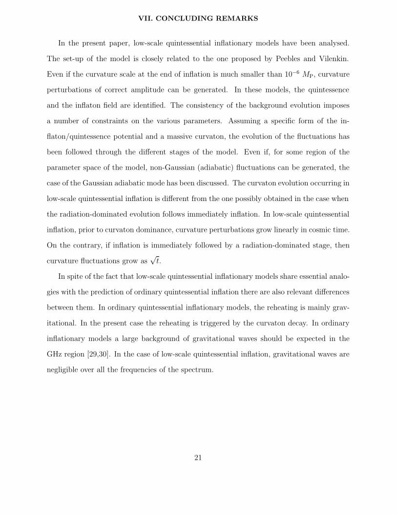
0 100 200 300 400 500 600 700 800 900 10000
1
2
3
4
5
6
7
8
9
M t
He =10−9 M
P
M =106 GeV
m = 107 GeV
He =10−11 M
P
M= 106 GeV
m =106 GeV
ϕ
100 200 300 400 500 600 700 800 900 1000−1
0
1x 10
−3
M t
ψ
He =10 −11 M
P
M =106 GeV
m = 106 GeV
ψe =0.001
FIG. 1. The result of the numerical integration of the background are illustrated for different
values of the parameters (indicated above each curve).
While the background is dominated by ϕ2, the field ψ slightly decreases with a rate given
by W,ψ. From Eq. (2.4), the field ψ slowly rolls toward the minimum of its potential in a
kinetic-energy-dominated environment and its approximate equation obeys
ψ ' − 1
6H
∂W
∂ψ, (2.12)
where the factor 1/6 comes from dropping consistently the terms of Eq. (2.4) containing
more than one derivative of the potential. This type of approximation has been exploited
in [13], but in the case of a slow-roll occurring during the radiation epoch.
Using Eq. (2.12), and recalling that a(t) ∼ t1/3, it can be checked that the evolution of
ψ slightly deviates from a constant value. For instance, in the case of a quadratic potential
the solution of Eq. (2.12) can be written as
ψ(t) ' ψe
[1− m2
4(t2 − t2e)
]. (2.13)
Equation (2.12) is useful in the case when the potential is more complicated than the
quadratic ansatz of Eq. (2.6) where Eq. (2.4) can be solved exactly. In fact, during
the kinetic regime the curvature scale decreases, and when H ∼ Hosc ∼ m the field ψ, still
subdominant, will start oscillating. The case of massive potential allows analytical solutions
of Eq. (2.4) during the kinetic phase for ψ:
5

ψ = ψe
√t
a3/2J0(mte)J0(mt), (2.14)
which leads to Eq. (2.12) in the limit mt� 1 and mte � 1. Since ψ decays as a−3/2 during
the oscillating regime, it will become dominant with respect to the kinetic energy of ϕ at a
scale
Hd ∼ 5 m( ψe
MP
)2
. (2.15)
The field ψ eventually decays at a curvature scale
Hr ∼ m3
M2P
. (2.16)
At Hm the potential of ϕ is still subdominant with respect to the kinetic energy. In fact
V (ϕm) ∼ λM4( M
MP
)4
ln−4(He
m
)� ϕ2
m
2' 1
9
(M2P
m2
), (2.17)
where the last equality comes from the kinetic term of ϕ at tm, evaluated on the basis of
Eq. (2.11). An example of the numerical integration is reported in Fig. 1. Furthermore,
the analytical evolution of ψ, as reported in Eq. (2.14), is in excellent agreement with the
numerical results.
Between Hd and Hr,
(ad
ar
)'
(mψe
)2
, (2.18)
the background geometry is effectively dominated by the oscillations of ψ, i.e. a(t) ∼ (mt)2/3.
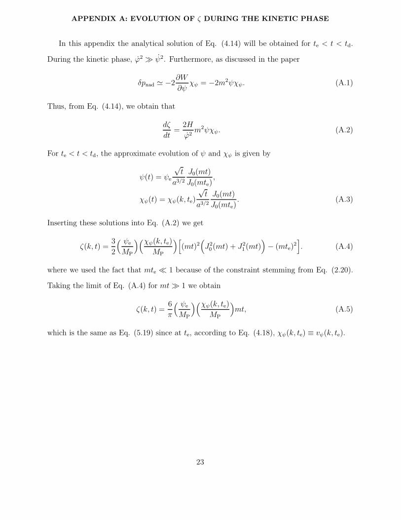
It is interesting to combine in the physical picture the constraints and the requirements
introduced so far. According to Eqs. (2.15) and (2.16) the quintessence field may become
subdominant either prior to or after the decay of ψ. In Fig. 2, with the (diagonal) dashed
line, the condition coming from the interplay between the decay of ψ and the dominance of
ϕ is illustrated for the specific case He ∼ 10−9MP. Above the dashed line, ψ decays during
the kinetic phase. Below, the dashed line the decay occurs when ψ already dominates. The
requirement of Eq. (2.10) also imposes a constraint on Fig. 2, implying that ψe and the
6

−18 −16 −14 −12 −10 −8 −6 −4 −2 0−18
−16
−14
−12
−10
−8
−6
−4
−2
0
log(
m/M
P)
log(ψe/M
P)
curvaton dominace
BBN bound
gaussianity
FIG. 2. The quantitative constraints pertaining to the combined analysis of the evolution of ψ
and ϕ during the kinetic phase are illustrated. With the dashed line the constraint coming from
the dominance of ψ is reported. The dot-dashed lined (from top to bottom) represent, respectively,
the bound (2.20) and the BBN bound. The full (vertical) line refers to Eq. (2.19). The shaded
region defines the allowed portion of the parameter space of the model.
7

mass should lie below the full fine in the right-hand corner. Consider now the situation
where the fluctuations of ψ are amplified, during inflation, with a scale-invariant spectrum.
Therefore, denoting by χψ the fluctuation of ψ, we do know that the power spectrum will
be δχψ ∼ He/2π. If
He
MP
< 2πψe
MP
, (2.19)
then the fluctuations of ψ will be predominantly Gaussian. In the opposite case they will
have some non-negligible non-Gaussian component. In order to have a nearly scale-invariant
spectrum for χψ, m should always be smaller than the curvature scale He. More precisely,
looking at the evolution equation for χψ (in conformal time) we are led to require
m <√
2He. (2.20)
Equation (2.20) is illustrated in Fig.2 with the dotted horizontal line. Finally, since the
decay of ψ should occur prior to BBN, an absolute lower bound on m, i.e. m > 10 TeV,
should be imposed. Therefore, already from these considerations it is possible to say that the
dashed area in Fig. 2 is allowed. Thus, the quintessence field has to become subdominant
before the decay of ψ if we want χψ to be Gaussian with nearly scale-invariant spectrum.
III. QUINTESSENTIAL EVOLUTION
In order to satisfy the physical constraints for the consistency of the scenario, it is
reasonable to require that the decay of ψ occur when ϕ is already sub dominant. If this is
the situation, Hd > Hr and, consequently,
ψe >∼1√5m. (3.1)
It is important, for the purposes of the present investigation, to analyse in some detail, the
evolution of ϕ around the curvature scales Hd and Hr.
After Hd, the evolution of ϕ results from the interplay between the smallness of its
potential term V (ϕ) and the coherent oscillations of ψ, which tend to make the average
8

expansion matter-dominated. The effect of the potential is, however, to introduce a growing
mode in the evolution of ϕ. This growing mode can be estimated by solving Eq. (2.3) with
the inverse power-law potential of Eq. (2.5). The solution is
ϕg(t) ' 31/3 λ1/6M4/3t1/3, td < t < tr. (3.2)
For t > tr, when the Universe is effectively radiation-dominated, a similar solution holds:
ϕg(t) '(72
5
)1/6
λ1/6M4/3t1/3, t > tr. (3.3)
The effective evolution of ϕ depends upon the balance of the growing mode with the
decaying modes obtained from Eq. (2.3) when the potential is neglected. During the regime
where ψ dominates and in the subsequent radiation-dominated regime, the evolution of ϕ is
given, respectively, by
ϕd(t) '√
2 MP
3
{[ln
(tdte
)+ 1
]− td
t
}, td < t < tr, (3.4)
ϕr(t) '√
2 MP
3
{[ln
(tdte
)+ 1 +
tdtr
]− 2
tdtr
√trt
}, t > tr. (3.5)
Equations (3.4) and(3.5) are continuous in tr. Furthermore Eqs. (2.11) and (3.4) are con-
tinuous in td. As obtained in [8] the growing solution never comes to dominate against the
decreasing mode. If
λ−1/2 ln3(tdte
)(MP
M
)4
>(H0
MP
)−1
, (3.6)
the growing mode becomes dominant only after the present expansion time t0 ∼ H−10 . We
will see that this condition is always verified because of the smallness of λ.
After tr the quintessence field is nearly constant and its potential energy is given by
V (ϕr) ' λM8
M4P
[ln
(tdte
)]−4
. (3.7)
The condition that the potential energy in the quintessence field is comparable with the
present energy density,
V (ϕr) ' H20M
2P, (3.8)
9

fixes a relation among M and λ
M
MP'
(9
2
)−1/4(H0
MP
)1/4
λ−1/8{
ln[√λ
5
(MP
m
)(MP
ψe
)2]}1/2
. (3.9)
Note that, for the typical parameters discussed so far, M is always greater than 105 GeV.
IV. LARGE SCALE FLUCTUATIONS
Having discussed the main features of the post-inflationary evolution, it is now mandatory
to understand the behaviour of the fluctuations. Available calculations on the curvaton
dynamics in different models [11–17] always deal with a post-inflationary phase, which is
dominated by radiation. Here, as discussed in the previous sections, the scenario is different.
Right after inflation the background evolution is not determined by radiation but by the
dynamics of ϕ, whose potential is now very steep. The fluctuation of the metric induced
by the fluctuations of ϕ will be, at the onset of the post-inflationary epoch, very small
since He < 10−6MP. Hence, had we to classify the metric fluctuations at te, we would say
that their modes are of the isocurvature type. However, as time goes by, the curvature
fluctuations, initially negligible at te, will be driven to a constant value so that, much later,
the initial isocurvature mode turns into an adiabatic one.
In order to describe this picture quantitatively, we are led to consider the coupled system
formed by the fluctuations of the metric and by the fluctuations of ϕ and ψ . The fluctuations
will then be discussed in the longitudinal gauge, where it is particularly simple to relate the
gauge-dependent quantities to gauge-invariant observables [20,21].
In the longitudinal gauge, the non-vanishing entries of the perturbed metric are
δg00 = 2φ, δgij = −2a2φ, (4.1)
where we used the fact that the fluctuations of the energy-momentum tensor are free of
shear. For the fluctuations of ϕ and ψ, in the longitudinal gauge the following notation will
also be adopted:
10

ϕ→ ϕ+ δϕ, δϕ = χϕ,
ψ → ψ + δψ, δψ = χψ. (4.2)
With these notations the evolution equations of the fluctuations can be written as
φ+ 4Hφ+ (2H + 3H2)φ = − 3
2M2P
[(ϕ2 + ψ)2φ− (ψχψ + ϕχϕ) +
∂V
∂ϕχϕ +
∂W
∂ψχψ
], (4.3)
3H(Hφ+ φ)− 1
a2∇2φ = − 3
2M2P
[−(ϕ2 + ψ)2φ+ (ψχψ + ϕχϕ) +
∂V
∂ϕχϕ +
∂W
∂ψχψ
], (4.4)
χϕ + 3Hχϕ − 1
a2∇2χϕ +
∂2V
∂ϕ2χϕ − 4ϕφ+ 2
∂V
∂ϕφ = 0, (4.5)
χψ + 3Hχψ − 1
a2∇2χψ +
∂2W
∂ψ2χψ − 4ψφ+ 2
∂W
∂ψφ = 0, (4.6)
where (4.3) and (4.4), come, respectively, from the (i, j) and (0, 0) components of the per-
turbed Einstein equations and (4.5) and (4.6) describe the evolution of the inhomogeneities
in the inflaton/quintessence field and in the curvaton field. Equations (4.3)–(4.6) are sub-
jected to the momentum constraint
Hφ+ φ =3
2M2P
(ϕχϕ + ψχψ). (4.7)
Using Eq. (4.7) together with Eqs. (4.3)–(4.6), it is possible to obtain a nicer form of the
perturbation equations [22–24,26]:
vϕ + 3Hvϕ − 1
a2∇2vϕ +
[∂2V
∂ϕ2− 3
M2Pa
3
∂
∂t
(a3
Hϕ2
)]vϕ − 3
M2Pa
3
∂
∂t
(a3
Hϕψ
)vψ = 0, (4.8)
vψ + 3Hvψ − 1
a2∇2vψ +
[∂2W
∂ψ2− 3
M2Pa
3
∂
∂t
(a3
Hψ2
)]vψ − 3
M2Pa
3
∂
∂t
(a3
Hϕψ
)vϕ = 0, (4.9)
where
vϕ = χϕ +ϕ
Hφ, (4.10)
vψ = χψ +ψ
Hφ. (4.11)
Eqs. (4.8) and (4.9) can be generalized to the case of an arbitrary number of fields [22,23]:
in this case the number of equations will clearly match the number of fields but the relative
structure of the equations will be the same.
11

Eqs. (4.4)–(4.6) or, equivalently, Eqs. (4.8) and(4.9), have to be studied and solved
along the different stages of the evolution of the background. In terms of vϕ and vψ, the
spatial curvature perturbation can be written as
ζ = − H
ϕ2 + ψ2[ϕvϕ + ψvψ]. (4.12)
The variable ζ is related also to φ by the usual expression
ζ =H
H(Hφ+ φ)− φ. (4.13)
Eq. (4.13) can be obtained from Eq. (4.12) (or vice versa) by using the momentum constraint
(4.7) expressed in terms of the of vϕ and vψ given in Eqs. (4.10) and (4.11).
An interesting (complementary) strategy in order to solve the system (4.3)–(4.6) and
(4.7) is to write down directly the evolution equation for ζ . Mutiplying Eq. (4.4) by the
sound of speed and subtracting it from Eq. (4.3) we obtain, at large scales [25],
dζ
dt= − H
ψ2 + ϕ2δpnad, (4.14)
where δpnad is, in our case,
δpnad = (c2s − 1)φ(ϕ+ ψ) + (1− c2s)(ϕχϕ + ψχψ)− (1 + c2s)(∂V∂ϕ
χϕ +∂W
∂ψχψ
), (4.15)
with
c2s =p
ρ= 1 +
2
3H(ϕ2 + ψ2)
(∂V∂ϕ
ϕ +∂W
∂ψψ
). (4.16)
In the first equality of Eq. (4.16) p and ρ are, respectively, the total pressure and energy
density of the system written in terms of the two background fields ϕ and ψ. Notice that in
order to get to (4.16) the background equations of motion (2.1)–(2.4) have been used.
The initial conditions of the system (4.4)–(4.6) after the end of inflation are dictated by
the smallness of λ. Going to Fourier space and considering only the super-horizon scales,
the initial conditions of the system are, for λ� 10−14,
φ(k, te) = 0, χϕ(k, te) = 0, χψ(k, te) =He
2π. (4.17)
12

In terms of vϕ and vψ, we have at the end of inflation, from Eqs. (4.8) and (4.9), on
super-horizon scales,
vϕ(k, te) = 0, vψ(k, te) = χψ(k, te), (4.18)
as is made clear by inserting Eqs. (4.17) into Eqs. (4.8) and (4.9). Physically Eqs. (4.17) and
(4.18) guarantee the absence of adiabatic modes at te. This aspect can also be appreciated
by looking at the initial conditions for ζ
ζ(k, te) = 0, (4.19)
as they follow from Eq. (4.12).
V. EVOLUTION DURING THE KINETIC PHASE
Using the initial conditions given by Eqs. (4.17)–(4.19), the evolution of the fluctuations
can be solved in slightly different but, ultimately, equivalent ways. In the following, as a first
step, the asymptotes for the evolution of the fluctuations will be discussed analytically in the
vicinity of te. The consistency of the analytical solutions with the results of the numerical
integration is an important check to be done. Following recent techniques developed in a
different framework [13], the solutions in the vicinity of te can be obtained without specifying
the form of the potential for the field ψ. Later on, in order to perform the numerical
integration, the case of massive potential will be mainly discussed.
A. The initial stages around te for generic potential
During this phase the field ψ slowly rolls down its own potential W (ψ), and the solution
to Eq. (2.4) is given by (2.12). The same expansion in the gradients of the potential W (ψ)
can be used in order to get the approximate evolution of the fluctuations.
Eqs. (4.8) and (4.9) can then be approximately solved by keeping the leading terms in the
derivatives of W (ψ). As done in the case of the background evolution, an equation analogous
13

to (2.12) can also be obtained for the canonical perturbation variable vψ. Eq. (4.9) can then
be expanded in gradients of the potential leading to the following approximate equation
vψ = − 1
6H
∂2W
∂ψ2vψ, (5.1)
whose solution implies that vψ is approximately constant. For instance, inserting into Eq.
(5.1) the explicit expression for W (ψ) given in Eq. (2.6), we get
vψ(k, t) ' vψ(k, te)[1− m2
4(t2 − t2e)
], t < tm. (5.2)
This expression has been verified numerically for various values of the physical parameters.
Using Eq. (5.2), Eq. (4.8) can be solved in the same approximation. Note, in fact, that
in Eq. (4.8) the term in square brackets is subleading with respect to the other terms for
two separate reasons. First V,ϕϕ is negligible in its own right, given the smallness of λ and
recalling that M/MP is O(10−13). Second, since a3ϕ2/H is constant, its time derivative
appearing in Eq. (4.8) is also negligible. The approximate evolution of vϕ(k, t) is then
given, at large scales, by
vϕ + 3Hvϕ − 3
M2Pa
3
∂
∂t
(a3
Hϕψ
)vψ = 0, (5.3)
whose solution, using Eqs. (2.12) and (5.1), becomes
vϕ(k, t) ' − 3
4M2P
( ϕH
)∂W∂ψ
vψ(k, t)[a6(t)− a6(te)]. (5.4)
Given that during the kinetic phase ϕ ' H , then vϕ(k, t) ∝ a6. Again, in the case of Eq.
(2.6), from Eq. (5.4) we obtain
vϕ(k, t) ' −3√
2
4
( ψe
MP
)m2(t2 − t2e)χψ(k, te), (5.5)
where, according to Eq. (4.18), vψ(k, te) = χψ(k, te) has been used. With the results of Eqs.
(5.2) and (5.5), from Eqs. (4.10)–(4.12) we can also obtain the approximate form of the
evolution of φk(t), ζk(t) and χϕ(k, t):
14

ζk(t) ' 3
2M2P
∂W
∂ψχψ(k, te)[a
6(t)− a6(te)], (5.6)
φk(t) ' − 3
10ζk(t), (5.7)
χϕ(k, t) ' − 3
10M2P
( ϕH
)∂W∂ψ
χψ[a6(t)− a6(te)]. (5.8)
The same results derived in Eqs. (5.6)–(5.8) and based on the solution of Eqs. (4.8) and
(4.9), with the initial conditions dictated by Eq. (4.18), can be obtained by integrating Eqs.
(4.4)–(4.6). As a check of the consistency of the approach, it is in fact useful to insert Eqs.
(5.7) and (5.8) back into Eqs. (4.3)–(4.6) and see that they are satisfied during the kinetic
phase and prior to the oscillations of ψ. Furthermore, the evolution of ζk, as obtained in
Eq. (5.6), can be also obtained directly from Eq. (4.14). In fact, during the kinetic phase
ψ � ϕ and, from Eq. (4.16) evaluated in the kinetic limit:
c2s ' 1− 1
18M2PH
4
∂W
∂ψ. (5.9)
Hence, from Eq. (4.15) we find
δpnad = −2∂W
∂ψχψ. (5.10)
Inserting (5.10) into Eq. (4.14) and performing the integral, we get exactly Eq. (5.6). The
analytic expressions derived so far allow a full control of the initial conditions of the system
in the vicinity of te.
B. Evolution for te < t < td
After the onset of the kinetic phase at te, but before the dominance of ψ at td, the
evolution of the system can be solved numerically for various sets of initial conditions; an
example of this behaviour is reported in Fig. 3 for the case of the potential given in Eq.
(2.6).
It will now be shown that the numerical evolution can be very accurately reproduced
analytically by direct integration of the evolution equation in a well defined approximation
15

10 20 30 40 50 60 70 80 90 100
−1.2
−1
−0.8
−0.6
−0.4
−0.2
0
0.2
0.4
0.6
0.8
x 10−8
m t
ζ
ζ
vψ
vφ
He = 10−8 M
P
ψ e
=0.01 MP
m = 10−3He
0 10 20 30 40 50 60 70 80 90 100−1.5
−1
−0.5
0
0.5
1
1.5x 10
−9
m t
ζ
ζ
vψ
vφ
He = 10−9 M
P
m = 10−3 He
ψ e
= 0.01 MP
FIG. 3. The result of the numerical integration for the evolution of the fluctuations are illus-
trated for the case M/MP = 10−13 and for a set of fiducial parameters chosen within the shaded
region of Fig. 2. In the left plot the analytical results (dashed lines) obtained in Eqs. (5.14), (5.17)
and (5.19) are compared with the numerical ones (full lines).
scheme. The evolution of the fluctuations will be analysed first using Eqs. (4.8) and (4.9)
and then using directly the evolution equation for ζ , i.e. Eq. (4.14).
In the case of the potential (2.6), Eqs. (4.8) and (4.9) can be written as
d
dt
(a3vϕ
)= −3
√2
MPm2ψvψ, (5.11)
vψ + 3Hvψ +m2[1 +
6
HM2P
ψψ]vψ +
3√
2
MP
m2ψvϕ = 0, (5.12)
where Eqs. (2.11) and (2.4) have been used. Recalling now the exact solution for the
evolution of (2.4), i.e. Eq. (2.14), it can be easily checked that, in Eq. (5.12):
6
HM2P
ψψ ∼ 18t
M2P
ψ2em < 1 (5.13)
for t < td ∼ m−1(MP/ψe)2. Neglecting the term containing vϕ in Eq. (5.12), the solution
for the evolution of vψ is given by
vψ(k, t) =vψ(k, te)
J0(xe)J0(x), (5.14)
where x = mt and J0(x) is the Bessel function of order 0 [27]. Eq. (5.14) reproduces exactly
the numerical solutions for vψ reported, for a particular case, in Fig. 3. Since it is always
16

true that mte � 1 for the constraints displayed in Fig. 2, the interesting limits of Eq. (5.14)
are for mt � 1 and mt � 1. In the limit mt � 1 Eq. (5.14) reproduces, as it should, the
time dependence obtained in Eq. (5.2). For mt� 1 we have [27], from Eq. (5.14):
vψ(k, t) = vψ(k, te)
√2
πxcos
(x− π
4
)(5.15)
Note the similarity between Eqs. (5.14) and (2.14), which is a simple consequence of the
quadratic form of the potential.
Inserting now Eq. (5.14) in Eq. (5.11), and integrating a first time between te and a
generic time t we get
dvϕdx
= − 3√
2
2MP
ψevψ(k, te)
J0(xe)
[x(J2
0 (x) + J21 (x)
)− F (xe)
x
], (5.16)
where F (xe) = x2e[J0(xe)
2 + J1(xe)2].
Direct integration of Eq. (5.16) implies that
vϕ(k, x) = −3√
2
4
ψevψ(k, te)
J0(xe)2
[x2
(J2
0 (x) + 2J21 (x)− J0(x)J2(x)
)−G(xe)− 2F (xe)
], (5.17)
where G(xe) = x2e [J
20 (xe)+ 2J2
1 (xe)−J0(xe)J2(xe)] and where, as usual, xe ∼ m/He. Taking
the limit for large x of Eq. (5.17) the following result can be obtained
vϕ(k, t) = −6√
2
πψevψ(k, te)(mt) +
3√
2
4ψevψ(k, te)(mte)
2 lnt
te, (5.18)
showing off the linear growth of vϕ with time.
Inserting now the solutions for vψ and vϕ given, respectively, in Eqs. (5.14) and (5.17)
into Eq. (4.12), the evolution of ζ for t < td, turns out to be, for mt > 1,
ζ(k, t) ' 6
π
( ψe
MP
)[vψ(k, te)
MP
](mt). (5.19)
Note that, for t = td, Eq. (5.19) gives
ζ(k, td) =2
5π
(vψ(k, te)
ψe
). (5.20)
Using the result of Eq. (5.19) into Eq. (4.13) the evolution for the large-scale modes of the
metric fluctuations can be obtained:
17

φ(k, t) ' −18
7π
( ψe
MP
)[vψ(k, te)
MP
](mt). (5.21)
Again we verified that the same results can be obtained directly by integrating the Hamil-
tonian constraint (4.4).
The time has come to compare the accuracy of the analytical expressions derived in Eqs.
(5.14), (5.17) and (5.19). These expressions have been plotted in Fig. 3 (left plot) with
the dashed lines. For the same set of parameters (and with the full line) the outcome of
the numerical integration has been reported. In the right plot the results for a different
set of parameters are displayed. The analytical expressions match rather accurately the
numerical results. Notice that the small wiggles in the evolution of ζ(k, t), modulating the
linear growth, are due to the fact that we decided to plot the full expression of ζ(k, t), which
contains Bessel functions, and not only its asymptotic limit for mt > 1. The same evolution
for ζ(k, t) derived in this section can be directly inferred from Eq. (4.14), recalling the
approximate form of δpnad. This calculation is reported in the appendix.
It is now appropriate to compare the situation of low-scale quintessential inflation with
the situation occurring in the more conventional case of curvaton models where the infla-
tionary phase is suddenly followed by the radiation-dominated phase. In this case the ζ(k, t)
variable grows as√t (i.e. linearly in conformal time) before the curvaton becomes domi-
nant. Here we found that the growth is linear in cosmic time. In spite of this difference,
the final amplitude of ζ(k, t) is given approximately by χψ(k, td)/ψe. In fact, in the case of
a quadratic potential evolving in a radiation-dominated environment,
ζ ∼( ψe
MP
)[χψ(k, teMP
]Ha(t), (5.22)
where we now have a(t) ∼ √t. Integrating once the previous formula we get ζ(k, t) ∼ √t.If the evolution occurs during radiation, the curvaton will become dominant at a typical
curvature scale Hd ∼ m(ψe/MP)4 [13]. Using this result, the amplitude of ζ(k, td) is given,
as previously anticipated, by χψ(k, td)/ψe.
18

VI. DOMINANCE OF ψ
Since ψ starts dominating the background at td, for t > td the evolution of the system is
described by the following set of equations
H2M2P =
[ ψ2
2+m2ψ2
], (6.1)
HM2P = −3
2ψ2, (6.2)
ψ + 3Hψ +m2ψ = 0. (6.3)
For large times Eqs. (6.1)–(6.3) lead to an effectively matter-dominated phase where the
oscillations of ψ,
ψ(t) ' ψ(td)cosmt
(Hdt)2, (6.4)
induce oscillations in the Hubble parameter and in the scale factor, which increases, on
average, as t2/3.
It is not difficult to see that, under these conditions, the evolution of vψ is dominated by
a constant mode. In Eq. (4.9) the term containing vϕ is always suppressed for large times
since,from Eq. (3.4)
ϕ '√
2
3MP
tdt2, (6.5)
and the quintessence field goes very rapidly to a constant. Thus, in this regime, the evolution
of vψ is given by
vψ(k, t) = vψ(k, td)ψ
H. (6.6)
Eq. (4.8) allows us to deduce that
vϕ(k, t) ∼ t−3. (6.7)
Inserting now Eqs. (6.4)–(6.7) into (4.12) we find that, for t > td, ζ is frozen to its constant
value. Therefore, right before the decay of ψ, the metric fluctuation will be given by
19

φ(k, tr) ∼ χψ(k, te)
ψe. (6.8)
After tr the field ψ decays and the evolution of the generated adiabatic mode becomes
standard, namely we have the fluctuations of the quintessence field evolving in a radiation-
dominated environment together with the constant mode of ζ . The evolution equations for
the fluctuations of the quintessence field will then obey, at large scales,
χϕ + 3Hχϕ +∂2V
∂ϕ2χϕ = 4ϕφ− 2
∂V
∂ϕφ. (6.9)
The other equations are the standard ones, namely
−3H(Hφ+ φ) =3
2M2P
ρrδr +3
2M2P
[−φϕ2 + ϕχϕ +
∂V
∂ϕχϕ
], (6.10)
φ+ 4Hφ+ (3H2 + 2H)φ =1
2M2P
ρrδr − 3
2M2P
[ϕ2φ− χϕ +∂V
∂ϕχϕ
](6.11)
Hφ+ φ =3
2M2P
[ϕχϕ +
4
3ρrur
], (6.12)
δr − 4φ = 0, (6.13)
ur − 1
4δr − φ = 0, (6.14)
where δr = δρr/ρr and ur is the velocity potential.
As discussed in the context of the quintessential evolution of the background, the
quintessence field, in the present model, does not lead to a tracking behaviour, as also
noticed in [8]. Thus, the evolution of the fluctuations during the radiation-dominated stage
of expansion will effectively be the one implied by a standard cosmological term. In fact we
can recall, from Eq. (3.5), that ϕ approaches a constant value as t−1/2 while the potential
is constant. Then, from Eq. (6.9) it can be deduced that also χϕ ∼ t−1/2 at large scales. As
a consequence, combining Eqs. (6.10) and (6.11) we have, at large scales,
φ+ 5Hφ+ 2(H + 2H2)φ = 0. (6.15)
leading to the usual constant mode which was present prior to matter-radiation equality, a
known feature of these types of models [28].
20
VII. CONCLUDING REMARKS
In the present paper, low-scale quintessential inflationary models have been analysed.
The set-up of the model is closely related to the one proposed by Peebles and Vilenkin.
Even if the curvature scale at the end of inflation is much smaller than 10−6 MP, curvature
perturbations of correct amplitude can be generated. In these models, the quintessence
and the inflaton field are identified. The consistency of the background evolution imposes
a number of constraints on the various parameters. Assuming a specific form of the in-
flaton/quintessence potential and a massive curvaton, the evolution of the fluctuations has
been followed through the different stages of the model. Even if, for some region of the
parameter space of the model, non-Gaussian (adiabatic) fluctuations can be generated, the
case of the Gaussian adiabatic mode has been discussed. The curvaton evolution occurring in
low-scale quintessential inflation is different from the one possibly obtained in the case when
the radiation-dominated evolution follows immediately inflation. In low-scale quintessential
inflation, prior to curvaton dominance, curvature perturbations grow linearly in cosmic time.
On the contrary, if inflation is immediately followed by a radiation-dominated stage, then
curvature fluctuations grow as√t.
In spite of the fact that low-scale quintessential inflationary models share essential analo-
gies with the prediction of ordinary quintessential inflation there are also relevant differences
between them. In ordinary quintessential inflationary models, the reheating is mainly grav-
itational. In the present case the reheating is triggered by the curvaton decay. In ordinary
inflationary models a large background of gravitational waves should be expected in the
GHz region [29,30]. In the case of low-scale quintessential inflation, gravitational waves are
negligible over all the frequencies of the spectrum.
21

ACKNOWLEDGMENTS
The author wishes to thank, V. Bozza, M. Gasperini and G. Veneziano for useful discus-
sions.
22
APPENDIX A: EVOLUTION OF ζ DURING THE KINETIC PHASE
In this appendix the analytical solution of Eq. (4.14) will be obtained for te < t < td.
During the kinetic phase, ϕ2 � ψ2. Furthermore, as discussed in the paper
δpnad ' −2∂W
∂ψχψ = −2m2ψχψ. (A.1)
Thus, from Eq. (4.14), we obtain that
dζ
dt=
2H
ϕ2m2ψχψ. (A.2)
For te < t < td, the approximate evolution of ψ and χψ is given by
ψ(t) = ψe
√t
a3/2
J0(mt)
J0(mte),
χψ(t) = χψ(k, te)
√t
a3/2
J0(mt)
J0(mte). (A.3)
Inserting these solutions into Eq. (A.2) we get
ζ(k, t) =3
2
( ψe
MP
)(χψ(k, te)MP
)[(mt)2
(J2
0 (mt) + J21 (mt)
)− (mte)
2]. (A.4)
where we used the fact that mte � 1 because of the constraint stemming from Eq. (2.20).
Taking the limit of Eq. (A.4) for mt� 1 we obtain
ζ(k, t) =6
π
( ψe
MP
)(χψ(k, te)MP
)mt, (A.5)
which is the same as Eq. (5.19) since at te, according to Eq. (4.18), χψ(k, te) ≡ vψ(k, te).
23

REFERENCES
[1] A. G. Riess et al., Astron. J. 116, 1009 (1998).
[2] S. Perlmutter et al., Astrophys. J. 517, 565 (1999).
[3] B. Ratra and J. Peebles, Phys. Rev. D 37, 3046 (1988).
[4] R. R. Caldwell, R. Dave, and P. J. Steinhardt, Phys. Rev. Lett. 80, 1582 (1998).
[5] L. Wang and P.J. Steinhardt, Astrophys.J. 508, 483 (1998).
[6] I. Zlatev, L. Wang, and P. J. Steinhardt, Phys. Rev. Lett. 82, 896 (1999 ).
[7] S. M. Carroll, Phys. Rev. Lett. 81, 3067 (1998).
[8] J. Peebles and A. Vilenkin, Phys. Rev. D 59, 063505 (1999).
[9] J. Peebles and A. Vilenkin, Phys. Rev. D 60, 103506 (1999).
[10] B. Spokoiny, Phys. Lett. B 315, 40 (1993).
[11] K. Enqvist and M. S. Sloth, Nucl. Phys. B626, 395 (2002).
[12] D. H. Lyth and D. Wands, Phys. Lett. B524, 5 (2002).
[13] V. Bozza, et al. Phys. Lett. B 543, 14 (2002); CERN/TH-2002-352, hep-ph/0212112.
[14] M. S. Sloth, hep-ph/0208241.
[15] T. Moroi and T. Takahashi, Phys. Lett. B 522, 15 (2001).
[16] M. Bastero-Gil, V. Di Clemente, and S.F. King, hep-ph/0211011
[17] C. Gordon, and A. Lewis, astro-ph/0212248
[18] S. Mollerach, Phys. Rev. D 42, 313 (1990).
[19] N. Bartolo and A. Liddle, Phys. Rev. D 65, 121301 (2002).
[20] V.F. Mukhanov, H.A. Feldman, and R. H. Brandenberger, Phys. Rep. 215, 203 (1992)..
24

[21] J. M. Bardeen, Phys. Rev. D22, 1882 (1980).
[22] J. Hwang, Phys. Rev. D 48, 3544 (1993); Class. Quant. Grav. 11, 2305 (1994).
[23] J. Hwang, Phys. Rev. D 53, 762 (1996); gr-qc/9608018.
[24] J. Hwang, Astrophys. J. 375, 443 (1991).
[25] H. Kodama and M. Sasaki, Prog. Theor. Phys. Suppl. 78, 1 (1984).
[26] A. Taruya and Y. Nambu, Phys. Lett. B 428, 37 (1998).
[27] A. Erdelyi, W. Magnus, F. Obehettinger, and F. R. Tricomi, Higher Trascendental
Functions (McGraw-Hill, New York, 1953).
[28] P. Viana and A. Liddle, Phys. Rev. D 57, 674 (1998)
[29] M. Giovannini, Class. Quant. Grav.16, 2905 (1999).
[30] M. Giovannini, Phys. Rev. D 60, 123511 (1999).
25