Embed Size (px)
Citation preview
www.elsevier.com/locate/geomorph
Geomorphology 72 (
Probabilistic landslide hazard assessment at the basin scale
Fausto Guzzetti *, Paola Reichenbach, Mauro Cardinali,
Mirco Galli, Francesca Ardizzone
IRPI CNR, via Madonna Alta 126, 06128 Perugia, Italy
Received 8 November 2004; received in revised form 24 May 2005; accepted 16 June 2005
Available online 15 August 2005
Abstract
We propose a probabilistic model to determine landslide hazard at the basin scale. The model predicts where landslides will
occur, how frequently they will occur, and how large they will be. We test the model in the Staffora River basin, in the northern
Apennines, Italy. For the study area, we prepare a multi-temporal inventory map through the interpretation of multiple sets of
aerial photographs taken between 1955 and 1999. We partition the basin into 2243 geo-morpho-hydrological units, and obtain
the probability of spatial occurrence of landslides by discriminant analysis of thematic variables, including morphological,
lithological, structural and land use. For each mapping unit, we obtain the landslide recurrence by dividing the total number of
landslide events inventoried in the unit by the time span of the investigated period. Assuming that landslide recurrence will
remain the same in the future, and adopting a Poisson probability model, we determine the exceedance probability of having
one or more landslides in each mapping unit, for different periods. We obtain the probability of landslide size by analysing the
frequency–area statistics of landslides, obtained from the multi-temporal inventory map. Assuming independence, we obtain a
quantitative estimate of landslide hazard for each mapping unit as the joint probability of landslide size, of landslide temporal
occurrence and of landslide spatial occurrence.
D 2005 Elsevier B.V. All rights reserved.
Keywords: Landslides; Mathematical model; Hazard; Susceptibility; Frequency; Magnitude; GIS; Maps
1. Introduction
Landslides are important natural hazards and an
active process that contributes to erosion and landscape
evolution. Different natural phenomena and human dis-
turbances trigger landslides. Natural triggers include
0169-555X/$ - see front matter D 2005 Elsevier B.V. All rights reserved.
doi:10.1016/j.geomorph.2005.06.002
* Corresponding author. Tel.: +39 075 501 4413; fax: +39 075
501 4420.
E-mail address: [email protected] (F. Guzzetti).
meteorological changes, such as intense or prolonged
rainfall or snowmelt, and rapid tectonic forcing, such as
earthquakes or volcanic eruptions. Human disturbances
include land use changes, deforestation, excavation,
changes in the slope profile, irrigation, etc. On Earth,
the volume of mass movements spans 15 orders of
magnitude, and landslide velocity extends over 14
orders of magnitude, from millimetres per year to hun-
dreds of kilometres per hour. Similarly,massmovements
can occur singularly or in groups of up to several thou-
2005) 272–299
F. Guzzetti et al. / Geomorphology 72 (2005) 272–299 273
sands. Multiple landslides, for example, occur almost
simultaneously when slopes are shaken by an earth-
quake, or over a period of hours or days when failures
are triggered by intense rainfall or snow melting. Land-
slides can involve flowing, sliding, toppling or falling
movements, and many landslides exhibit a combination
of these types of movements (Cruden and Varnes,
1996). The extraordinary breadth of the spectrum of
landslides makes it difficult to define a single metho-
dology to ascertain landslide hazard (Guzzetti, 2002).
Many methods have been proposed to evaluate
quantitatively landslide hazard geographically at the
basin scale (Carrara, 1983; Carrara et al., 1991, 1995;
van Westen, 1994; Soeters and van Westen, 1996;
Chung and Frabbri, 1999; Guzzetti et al., 1999 and
references herein). Such models are best classified as
susceptibility models (Brabb, 1984), because they pro-
vide an estimate of bwhereQ landslides are expected. Afew attempts have been made to establish the temporal
frequency of slope failures (Keaton et al., 1988; Lips
and Wieczorek, 1990; Coe et al., 2000; Crovelli, 2000;
RIVANAZZANO
Piedmont
Lombardy
Emilia-RomagnaTURIN
MILAN
BOLOGN
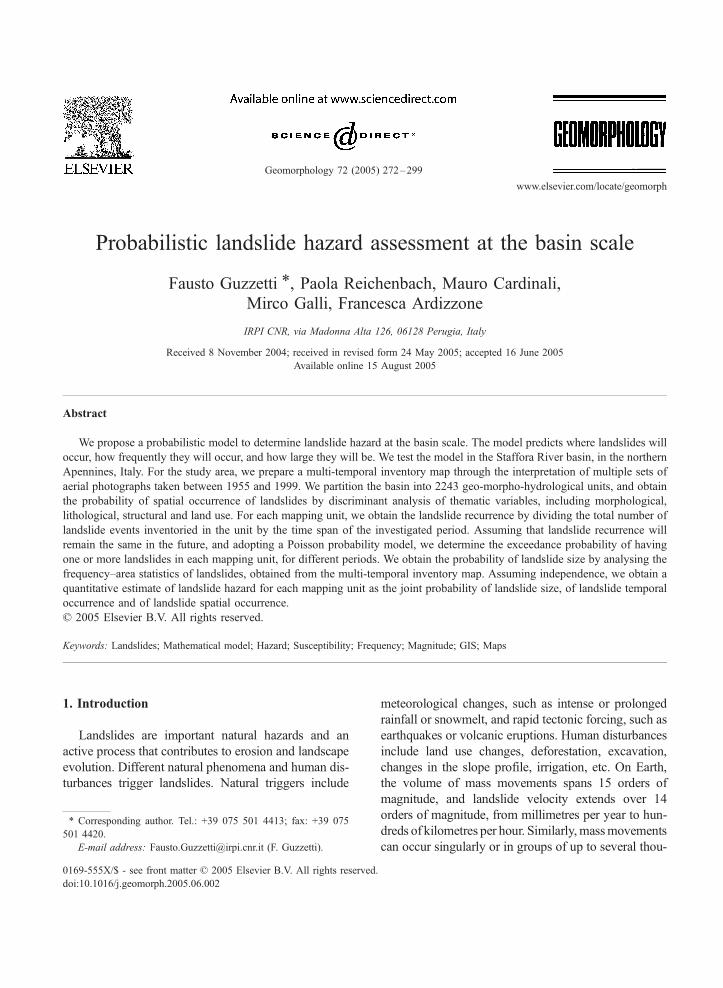
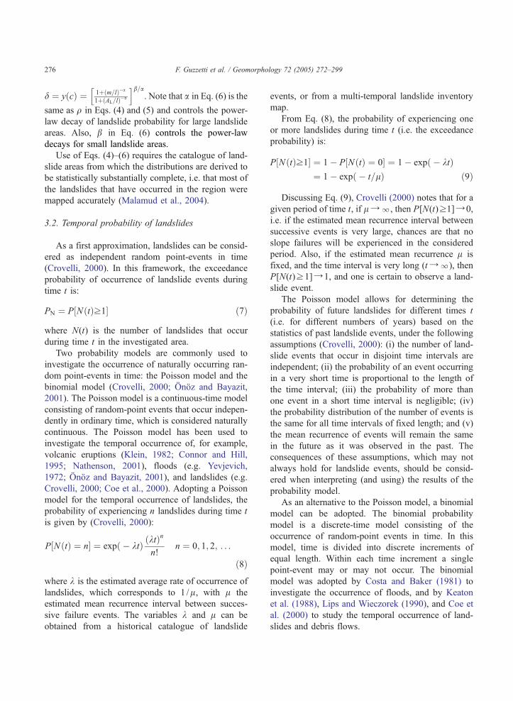
Fig. 1. Location of the study area
Guzzetti et al., 2002a,b). The latter models attempt to
predict bwhenQ a landslide will occur by establishing
the exceedance probability of landslide occurrence
during an established period. Most commonly, the
exceedance probability is obtained from catalogues
of historical landslide events, which are lists showing
the time (or period) of occurrence of single or multiple
slope failures. No single measure of landslide magni-
tude exists (Guzzetti, 2002). For certain landslide
types, including slides and complex failures, landslide
area is a reasonable proxy for landslide magnitude.
Recently, information has become available on the
frequency–area statistics of landslides (Hovius et al.,
1997; Stark and Hovius, 2001; Guzzetti et al., 2002a,b;
Guthrie and Evans, 2004a,b; Malamud et al., 2004).
This information can be used to determine the
expected probability of landslide area and magnitude.
In this paper, we propose a probabilistic model to
determine landslide hazards at the basin scale. The
model exploits information obtained from a multi-
temporal inventory map to predict where landslides
VARZI
M. CHIAPPA
A
N0 2 4 km1
, the Staffora River basin.
F. Guzzetti et al. / Geomorphology 72 (2005) 272–299274
will occur, how frequently they will occur, and how
large they will be. We test this model in the Staffora
River basin, in the Northern Apennines, and we dis-
cuss the results obtained.
2. The study area
The study area extends for 275 km2 in the southern
Lombardy region, in northern Italy (Fig. 1). Elevation
in the area ranges from about 150 m at Rivanazzano to
1699 m at M. Chiappa. The Staffora River, a tributary
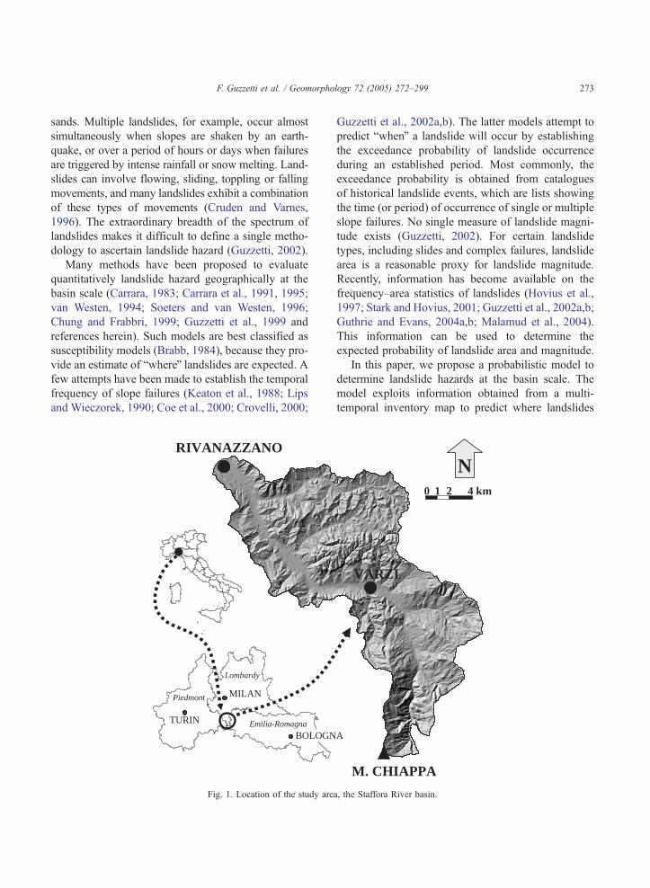
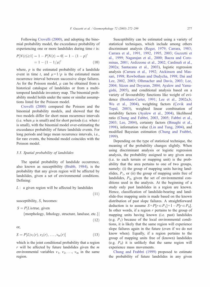
of the Po River, drains the area. In the 42-year period
from 1951 to 1991, annual rainfall in the area ranged
from 410 to 1357 mm, with an average value of 802
mm. Precipitation is most abundant in the autumn and
in the spring (Fig. 2).
Marine, transitional and continental sedimentary
rocks, Cretaceous to Holocene in age (Servizio Geo-
logico Nazionale, 1971) outcrop in the Staffora River
basin. Marine sediments include: (i) sequences of
layered limestone, marly-limestone, marl and clay,
with ophiolites, (ii) disorganized, and highly fractured
marl and clay, overlaid by massive sandstones, and
(iii) shallow marine sediments pertaining to the Ges-
soso-Solfifera Fm. Transitional deposits feature con-
glomerates, with lenses of marl and sand, which are
Oligocene in age. Fluvial and terraced deposits, Holo-
cene in age, represent the continental deposits and
outcrop along the main valley bottoms.
The area has a complex structural setting resulting
from the superposition of two tectonic phases asso-
20
40
60
80
100
Jan
Feb
Mar
Apr
May Jun
Jul
Aug Sep
Oct
Nov
Dec
Mea
n m
onth
ly r
ainf
all (
mm
)
2
4
6
8
10
12
14
Perc
enta
ge o
f m
ean
annu
al r
ainf
all (
%)
Fig. 2. Monthly rainfall values (left y-axis) and percentages (right y-
axis) for the period between 1951 and 1990 for the Varzi rain gauge,
416 m a.s.l.
ciated to the formation of the Apennines mountain
chain. A compressive phase of Cretaceous to Eocene
age produced large, north–east verging thrusts with
associated anticlines, synclines and transcurrent faults,
and was followed by an extensional tectonic phase of
Oligocene to Holocene age, which produced chiefly
normal faults. The lithological and the structural set-
tings control the morphology of the area, which fea-
tures steep and asymmetric slopes, dissected by a
dense, locally actively eroding stream network. Land-
slides are abundant in the area, and range in type and
size from large rotational and translational slides to
deep and shallow flows. Some of the landslides are
presumably very old in age. Very old landslides are
mostly relict or dormant, and are partially concealed
by forest and the intensive farming activity.
3. Mathematical model
Varnes and the IAEG Commission on Landslides
and other Mass-Movements (1984) proposed that the
definition adopted by the United Nations Disaster
Relief Organization (UNDRO) for all natural hazards
be applied to the hazard posed by mass movements.
Varnes and his co-workers defined the landslide
hazard as bthe probability of occurrence within a
specified period of time and within a given area of a
potentially damaging phenomenonQ. Guzzetti et al.
(1999) amended the definition to include the magni-
tude of the event. In contrast to other natural hazards,
no unique measure of landslide magnitude is available
(Hungr, 1997). For earthquakes, magnitude is a mea-
sure of the energy released during an event. For land-
slides, a measure of the energy released during failure
is difficult to obtain. Hungr (1997) proposed destruc-
tiveness to be a measure of landslide magnitude.
Cardinali et al. (2002b) and Reichenbach et al.
(2005) defined landslide destructiveness as a function
of the landslide volume and of the expected landslide
velocity, the latter obtained from the landslide type.
For large areas, landslide volume and velocity are
difficult to evaluate systematically, making the
approach impracticable. Alternatively, where slope
failures are chiefly slow-moving slides and slide
earth-flows, destructiveness can be related to the
area of the landslide, information that is readily avail-
able from accurate landslide inventory maps.
F. Guzzetti et al. / Geomorphology 72 (2005) 272–299 275
The definition of landslide hazard incorporates the
concepts of location, time and size. To complete a
hazard assessment one has to predict (quantitatively)
bwhereQ a landslide will occur, bwhenQ or how fre-
quently it will occur, and bhow largeQ the landslide
will be. In mathematical terms, this can be written as:
HL ¼ P½ALzaLin a time interval t; given
fmorphology; lithology; structure; landuse; . . . g�ð1Þ
where, AL is the area of a landslide greater or equal
than a minimum size, aL, measured, for example, in
square meters. For any given area, Eq. (1) expresses
landslide hazard as the conditional probability of land-
slide size, PAL, of landslide occurrence in an estab-
lished period t, PN, and of landslide spatial
occurrence, S, given the local environmental setting.
Assuming independence among the three probabil-
ities, the landslide hazard, i.e. the joint probability is:
HL ¼ PAL� PN � S ð2Þ
From a geomorphological point of view, the
assumption that the three probabilities (i.e., the three
components of landslide hazard) are independent is
strong and may not hold always and everywhere. In
many areas we expect slope failures to be more fre-
quent (time component) where landslides are more
abundant and landslide area is large (spatial compo-
nent). However, given the lack of understanding of the
landslide phenomena, independence is an acceptable
first-approximation that makes the problem mathema-
tically tractable and easier to work with.
3.1. Probability of landslide size
The probability that a landslide will have an area
greater or equal than aL is:
PAL¼ P ALzaL½ � ð3Þ
and can be estimated from the analysis of the fre-
quency–area distribution of known landslides,
obtained from landslide inventory maps. Analysis of
accurate landslide inventories reveals that the abun-
dance of landslides increases with landslide area up to
a maximum value, where landslides are most frequent,
then it decays rapidly along a power law (Pelletier et
al., 1997; Hovius et al., 1997; Stark and Hovius, 2001;
Guzzetti et al., 2002a,b; Guthrie and Evans, 2004a,b;
Malamud et al., 2004).
Malamud et al. (2004) analysed three recent and
well documented landslide inventories from California
(Harp and Jibson, 1996), central Italy (Cardinali et al.,
2000; Guzzetti et al., 2002a,b) and Guatemala (Buck-
nam et al., 2001), and found the probability density
function (PDF) of landslide area, AL, to be in good
agreement with a truncated inverse gamma distribu-
tion. These authors proposed that the PDF of landslide
area can be estimated as (Malamud et al., 2004):
p AL; q; a; sð Þ ¼ 1
aC qð Þa
AL s
� �qþ1
exp a
AL s
� �ð4Þ
where: C(q) is the gamma function of q, and q N0,
aN0, and sVALbl are parameters of the distribution.
In Eq. (4), q controls the power–law decay for medium
and large landslide areas, a primarily controls the
location of the maximum of the probability distribu-
tion, and s primarily controls the exponential decay for
small landslide areas. Fitting Eq. (4) to the three avail-
able inventories, Malamud et al. (2004) found
q =1.40, a =1.28d 103 m2, and s=1.32d 102 m2
(determination coefficient r2=0.965).
Using Eq. (4), PALis given by:
PAL¼Z l
aL
p AL; q; a; sð ÞdAL ¼Z l
aL
1
aC qð Þa
AL s
� �qþ1
� exp a
AL s
� �dAL ð5Þ
In another study of frequency–area statistics of
landslides, Stark and Hovius (2001) analyzed three
landslide datasets obtained from New Zealand and
Taiwan and found the PDF of landslide area to be in
good agreement with a double Pareto probability dis-
tribution. Using this distribution, PALis given by (Stark
and Hovius, 2001):
PAL¼
Z l
aL
p AL; a; b; l;m; cð ÞdAL
¼Z l
aL
bl 1 dð Þ
1þ m=lð Þa½ �b=a
1þ AL=lð Þa½ �1þ b=að Þ
" #
� AL=lð Þ aþ1ð ÞdAL ð6Þ
where: a N0, b N0, 0VcV lVmVl, and with
F. Guzzetti et al. / Geomorphology 72 (2005) 272–299276
d ¼ y cð Þ ¼ 1þ m=lð Þa
1þ AL=lð Þa
h ib=a. Note that a in Eq. (6) is the
same as q in Eqs. (4) and (5) and controls the power-
law decay of landslide probability for large landslide
areas. Also, b in Eq. (6) controls the power-law
decays for small landslide areas.
Use of Eqs. (4)–(6) requires the catalogue of land-
slide areas from which the distributions are derived to
be statistically substantially complete, i.e. that most of
the landslides that have occurred in the region were
mapped accurately (Malamud et al., 2004).
3.2. Temporal probability of landslides
As a first approximation, landslides can be consid-
ered as independent random point-events in time
(Crovelli, 2000). In this framework, the exceedance
probability of occurrence of landslide events during
time t is:
PN ¼ P N tð Þz1½ � ð7Þ
where N(t) is the number of landslides that occur
during time t in the investigated area.
Two probability models are commonly used to
investigate the occurrence of naturally occurring ran-
dom point-events in time: the Poisson model and the
binomial model (Crovelli, 2000; Onoz and Bayazit,
2001). The Poisson model is a continuous-time model
consisting of random-point events that occur indepen-
dently in ordinary time, which is considered naturally
continuous. The Poisson model has been used to
investigate the temporal occurrence of, for example,
volcanic eruptions (Klein, 1982; Connor and Hill,
1995; Nathenson, 2001), floods (e.g. Yevjevich,
1972; Onoz and Bayazit, 2001), and landslides (e.g.
Crovelli, 2000; Coe et al., 2000). Adopting a Poisson
model for the temporal occurrence of landslides, the
probability of experiencing n landslides during time t
is given by (Crovelli, 2000):
P N tð Þ ¼ n½ � ¼ exp ktð Þ ktð Þn
n!n ¼ 0; 1; 2; . . .
ð8Þ
where k is the estimated average rate of occurrence of
landslides, which corresponds to 1 /l, with l the
estimated mean recurrence interval between succes-
sive failure events. The variables k and l can be
obtained from a historical catalogue of landslide
events, or from a multi-temporal landslide inventory
map.
From Eq. (8), the probability of experiencing one
or more landslides during time t (i.e. the exceedance
probability) is:
P N tð Þz1½ � ¼ 1 P N tð Þ ¼ 0½ � ¼ 1 exp ktð Þ¼ 1 exp t=lð Þ ð9Þ
Discussing Eq. (9), Crovelli (2000) notes that for a
given period of time t, if lYl, then P[N(t)z1]Y0,
i.e. if the estimated mean recurrence interval between
successive events is very large, chances are that no
slope failures will be experienced in the considered
period. Also, if the estimated mean recurrence l is
fixed, and the time interval is very long (tYl), then
P[N(t)z1]Y1, and one is certain to observe a land-
slide event.
The Poisson model allows for determining the
probability of future landslides for different times t
(i.e. for different numbers of years) based on the
statistics of past landslide events, under the following
assumptions (Crovelli, 2000): (i) the number of land-
slide events that occur in disjoint time intervals are
independent; (ii) the probability of an event occurring
in a very short time is proportional to the length of
the time interval; (iii) the probability of more than
one event in a short time interval is negligible; (iv)
the probability distribution of the number of events is
the same for all time intervals of fixed length; and (v)
the mean recurrence of events will remain the same
in the future as it was observed in the past. The
consequences of these assumptions, which may not
always hold for landslide events, should be consid-
ered when interpreting (and using) the results of the
probability model.
As an alternative to the Poisson model, a binomial
model can be adopted. The binomial probability
model is a discrete-time model consisting of the
occurrence of random-point events in time. In this
model, time is divided into discrete increments of
equal length. Within each time increment a single
point-event may or may not occur. The binomial
model was adopted by Costa and Baker (1981) to
investigate the occurrence of floods, and by Keaton
et al. (1988), Lips and Wieczorek (1990), and Coe et
al. (2000) to study the temporal occurrence of land-
slides and debris flows.
F. Guzzetti et al. / Geomorphology 72 (2005) 272–299 277
Following Crovelli (2000), and adopting the bino-
mial probability model, the exceedance probability of
experiencing one or more landslides during time t is:
P N tð Þz1½ � ¼ 1 P N tð Þ ¼ 0½ � ¼ 1 1 pð Þt
¼ 1 1 1=lð Þt ð10Þ
where, p is the estimated probability of a landslide
event in time t, and l =1 /p is the estimated mean
recurrence interval between successive slope failures.
As for the Poisson model, l can be obtained from a
historical catalogue of landslides or from a multi-
temporal landslide inventory map. The binomial prob-
ability model holds under the same or similar assump-
tions listed for the Poisson model.
Crovelli (2000) compared the Poisson and the
binomial probability models, and showed that the
two models differ for short mean recurrence intervals
(i.e. when l is small) and for short periods (i.e. when t
is small), with the binomial model over-estimating the
exceedance probability of future landslide events. For
long periods and large mean recurrence intervals, i.e.,
for rare events, the bimodal model coincides with the
Poisson model.
3.3. Spatial probability of landslides
The spatial probability of landslide occurrence,
also known as susceptibility (Brabb, 1984), is the
probability that any given region will be affected by
landslides, given a set of environmental conditions.
Defining:
L : a given region will be affected by landslides
ð11Þ
susceptibility, S, becomes:
S ¼ P L is true; given½fmorphology; lithology; structure; landuse; etc:g�
ð12Þ
or,
S ¼ P Ljv1 rð Þ; v2 rð Þ; . . . ; vm rð Þ½ � ð13Þ
which is the joint conditional probability that a region
r will be affected by future landslides given the m
environmental variables v1, v2, . . ., vm in the same
region.
Susceptibility can be estimated using a variety of
statistical techniques, which include among others
discriminant analysis (Reger, 1979; Carrara, 1983;
Carrara et al., 1991, 1992, 1995, 2003; Guzzetti et
al., 1999; Nagarajan et al., 2000; Baeza and Coro-
minas, 2001; Ardizzone et al., 2002; Cardinali et al.,
2002a; Santacana et al., 2003), logistic regression
analysis (Carrara et al., 1992; Atckinson and Mas-
sari, 1998; Rowbotham and Dudycha, 1998; Dai and
Lee, 2002, 2003; Olhmacher and Davis, 2003; Lee,
2004; Suzen and Doyuran, 2004; Ayalew and Yama-
gishi, 2005), and conditional analysis based on a
variety of favourability functions like weight of evi-
dence (Bonham-Carter, 1991; Lee et al., 2002a,b;
Wu et al., 2004), weighting factors (Cevik and
Topal, 2003), weighted linear combination of
instability factors (Ayalew et al., 2004), likelihood
ratio (Chung and Fabbri, 2003, 2005; Fabbri et al.,
2003; Lee, 2004), certainty factors (Binaghi et al.,
1998), information value (Lin and Tung, 2004), and
modified Bayesian estimation (Chung and Frabbri,
1999).
Depending on the type of statistical technique, the
meaning of the probability changes slightly. When
using discriminant analysis or logistic regression
analysis, the probability assigned to any given area
(i.e. to each terrain or mapping unit) is the prob-
ability that the area pertains to one of two groups,
namely: (i) the group of mapping units having land-
slides, P1, or (ii) the group of mapping units free of
landslides, P0, given the set of environmental con-
ditions used in the analysis. At the beginning of a
study only past landslides in a region are known.
Hence, classification of landslide-bearing and land-
slide-free mapping units is made based on the known
distribution of past slope failures. A straightforward
deduction is to assume S =P[raP1]=1P[raP0].
In other words, if a region r pertains to the group of
mapping units having known (i.e. past) landslides
(e.g. P1) because of the local environmental condi-
tions, it is likely that the same region will experience
slope failures again in the future (even if we do not
know when). Equally, if a region pertains to the
group of mapping units free of (known) landslides
(e.g. P0) it is unlikely that the same region will
experience mass movements.
Chung and Frabbri (1999) proposed to estimate
the probability of future landslides in any given
F. Guzzetti et al. / Geomorphology 72 (2005) 272–299278
region, S, from the probability of past landslides in
the same region, given a set of environmental vari-
ables. Letting:
F : a given region has been affected by landslides;
ð14Þ
the joint conditional probability of past landslides in
a region r, given the m environmental variables v1,
v2, . . ., vm in the same region is:
D ¼ P Fjv1 rð Þ; v2 rð Þ; . . . ; vm rð Þ½ � ð15Þ
From Eqs. (13) and (15) it follows that:
P Ljv1 rð Þ; v2 rð Þ; . . . ; vm rð Þ½ � ¼ P Fjv1 rð Þ;½v2 rð Þ; . . . ; vm rð Þ�; ð16Þ
or S =D. To estimate the spatial probability of past
landslides (and infer from it the spatial probability
of future failures), the study area is partitioned into
unique condition units (UCU), i.e. areas character-
ized by an exclusive (unique) combination of envir-
onmental conditions. This can be easily obtained in
a GIS by the geographical union of all thematic
layers available for the study area. The spatial
probability of past landslide occurrence is then sim-
ply estimated from the density of landslides in each
UCU.
Chung and Frabbri (1999) showed that D is a
good descriptor of the past (known) landslides,
conditioned to the available environmental informa-
tion, but it may not be a good estimator of the
future spatial occurrence of landslides, S. They
proposed more efficient indexes to estimate the
future occurrence of landslides from the observed
past distribution of slope failures, including: (i) a
Bayesian estimation under the condition of indepen-
dence, (ii) a regression model based on bivariate
conditional probabilities, (iii) a modified Bayesian
estimator under the condition of independence, and
(iv) a modified regression model based on bivariate
conditional probabilities. The two modified models
incorporate expert knowledge, i.e. information
which is not included in the original landslide or
thematic data, and that is used to modify the
observed frequency of occurrence of landslides to
fit the expert’s understanding of landslide phenom-
ena (Chung and Frabbri, 1999). This is an improve-
ment over other modelling approaches, particularly
where information on past landslides is limited or
imprecise.
Quantitative susceptibility models can predict the
spatial occurrence of future landslides under the gen-
eral assumption that in any given area slope failures
will occur in the future under the same circumstances
and because of the same conditions that caused them
in the past. This is a geomorphological rephrase of
bthe past is the key to the futureQ, which is a direct
consequence of the well-known principle of unifor-
mitarianism. However, the principle may not hold for
landslides. New, first-time failures occur under con-
ditions of peak resistance (friction and cohesion),
whereas reactivations occur under intermediate or
residual conditions. It is well known that terrain
gradient is an important factor for the occurrence of
landslides. An obvious effect of a slope failure is to
change the morphology of the terrain where the fail-
ure occurs. In addition, when a landslide moves it
may change the hydrological conditions of the slope.
It is also well known that landslides can change their
type of movement and velocity with time. Lastly,
landslide occurrence and abundance are a function
of environmental conditions that vary with time at
different rates. Some of the environmental variables
are affected by human actions (e.g. land use, defor-
estation, irrigation, etc.), which are also highly
changeable. Because of these complications, each
landslide occurs in a distinct environmental context,
which may have been different in the past and that
might be different in the future. Despite these limita-
tions, in this work we assume that the principle of
uniformity hold bstatisticallyQ, i.e. that in the investi-
gated region future landslides will occur on average
under the same circumstances and because of the
same conditions that triggered them in the past. We
further assume that our knowledge of the distribution
of past failures is reasonably accurate and complete.
We accept these simplifications to make the problem
tractable.
4. Landslide hazard assessment
To ascertain landslide hazard we partitioned the
Staffora basin into mapping units (Guzzetti et al.,
F. Guzzetti et al. / Geomorphology 72 (2005) 272–299 279
1999), adopting the procedure proposed by Carrara
et al. (1991). Starting from a digital terrain model
with a ground resolution of 20 m�20 m and a
simplified representation of the main drainage lines,
specialized software (Carrara et al., 1991; Detti and
Pasqui, 1995) was used to partition the territory
into individual slope units, bounded by drainage
and divide lines. For each slope unit, the software
computed 21 morphometric and hydrological para-
meters useful in explaining the spatial distribution
of landslides (Carrara et al., 1991, 1995). We
further subdivided the slope units according to the
main rock types cropping out in the basin. In this
way, we partitioned the study area into 2243 map-
ping units based on lithology, morphology and
hydrology (geo-morpho-hydrological terrain units),
which represent the mapping units used for the
hazard assessment.
4.1. Landslide identification and mapping
We obtained information on the geographical and
temporal distribution of landslides and on landslide
size from a detailed multi-temporal inventory map,
prepared through the interpretation of multiple sets
of aerial photographs. For the study area, five sets of
aerial photographs were available to us (Table 1). We
used each set of aerial photographs separately to
obtain different landslide inventory maps (Fig. 3).
We then merged in a GIS the five individual land-
slide maps to obtain the multi-temporal inventory
map (Fig. 3F).
Table 1
Staffora River basin
Code Flight Date Type Nominal scale
A GAI-IGMI 18 July
1955
Black and
white
1 :33,000
B ALI FOTO Winter
1975
Black and
white
1 :15,000
C TEM 1 Summer
1980
Colour 1 :22,000
D Lombardy Summer
1994
Black and
white
1 :25,000
E IT 2000 22 June
1999
Colour 1 :40,000
Aerial photographs used to compile the multi-temporal landslide
inventory map.
A team of three geomorphologists carried out inter-
pretation of the aerial photographs in a period of 6
months. Two team members looked at each pair of
aerial photographs using a mirror stereoscope (with a
magnification of 4�) that allowed both interpreters to
map contemporaneously on the same stereo pair. The
third photo-interpreter independently reviewed, and
where necessary corrected the interpretations of the
other two, using a high magnification (up to 20�)
stereoscope. For the interpretation, we used all geolo-
gical and geomorphological information available to
us from published maps, previous works carried out in
the same area, and discussion with other geologists
(Rossetti, 1997; Antonini et al., 2000; Ardizzone et
al., 2002).
Landslide information collected through the inter-
pretation of aerial photographs was visually trans-
ferred to topographic maps at 1 :10,000 scale. We
transferred geomorphological information from the
base maps onto stable, transparent sheets and scanned
these to obtain black and white, raster images of each
map sheet. We used a scanning resolution of 300–400
dpi, which corresponded to a ground resolution of less
than 0.1 m. The raster representation of the geomor-
phological line images was changed in a GIS into
vector format using a semi-automatic procedure,
which allowed us to assign attributes to each line
segment. Polygons were then constructed and labelled
with the appropriate codes, depending on their land-
slide properties.
In the separate inventory maps (Fig. 3A–E), we
classified landslides according to the type of move-
ment, and the estimated age, activity, depth, and
velocity. We defined landslide type according to
Cruden and Varnes (1996), and the WP/WLI
(1990). For deep-seated slope failures, we mapped
separately the landslide crown (depletion area) from
the deposit. Landslide age, activity, depth, and
velocity were determined based on the type of
movement, the morphological characteristics and
appearance of the landslide on the aerial photo-
graphs, the local lithological and structural setting,
and the date of the aerial photographs. We categor-
ized landslide age as recent, old or very old,
despite ambiguity in the definition of the age of a
mass movement based on its appearance (Wiec-
zorek, 1984). Landslides were classified active
(WP/WLI, 1993) where they appeared fresh on
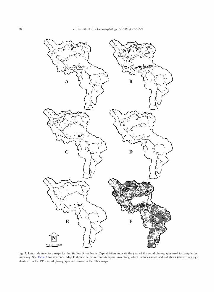
Fig. 3. Landslide inventory maps for the Staffora River basin. Capital letters indicate the year of the aerial photographs used to compile the
inventory. See Table 2 for reference. Map F shows the entire multi-temporal inventory, which includes relict and old slides (shown in grey)
identified in the 1955 aerial photographs not shown in the other maps.
F. Guzzetti et al. / Geomorphology 72 (2005) 272–299280
F. Guzzetti et al. / Geomorphology 72 (2005) 272–299 281
the aerial photographs (of a given date). Mass move-
ments were classified as deep-seated or shallow,
depending on the type of movement and the estimated
landslide volume. The latter was based on the type of
failure, and the morphology and geometry of the
detachment area and the deposition zone. Landslide
velocity (WP/WLI, 1995; Cruden and Varnes, 1996)
was considered a proxy of landslide type, and classi-
fied accordingly. We acknowledge that the adopted
classification scheme suffers from simplifications and
required geomorphological deduction, but it fits the
available information on landslide types and process in
the northern Apennines (Rossetti, 1997).
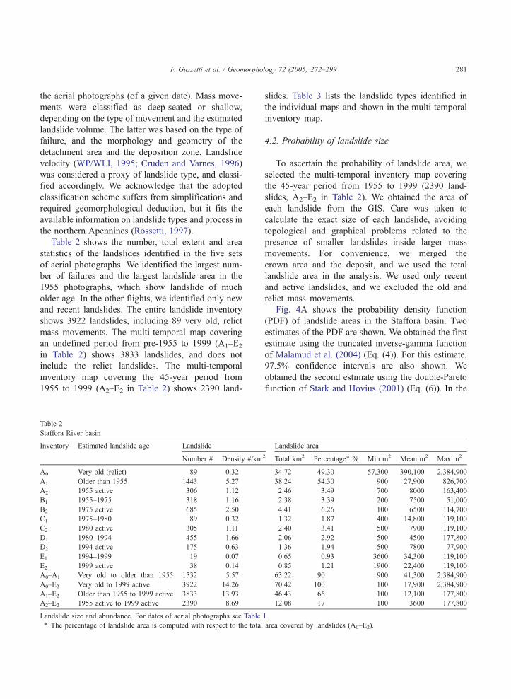
Table 2 shows the number, total extent and area
statistics of the landslides identified in the five sets
of aerial photographs. We identified the largest num-
ber of failures and the largest landslide area in the
1955 photographs, which show landslide of much
older age. In the other flights, we identified only new
and recent landslides. The entire landslide inventory
shows 3922 landslides, including 89 very old, relict
mass movements. The multi-temporal map covering
an undefined period from pre-1955 to 1999 (A1–E2
in Table 2) shows 3833 landslides, and does not
include the relict landslides. The multi-temporal
inventory map covering the 45-year period from
1955 to 1999 (A2–E2 in Table 2) shows 2390 land-
Table 2
Staffora River basin
Inventory Estimated landslide age Landslide
Number # Density #/km
A0 Very old (relict) 89 0.32
A1 Older than 1955 1443 5.27
A2 1955 active 306 1.12
B1 1955–1975 318 1.16
B2 1975 active 685 2.50
C1 1975–1980 89 0.32
C2 1980 active 305 1.11
D1 1980–1994 455 1.66
D2 1994 active 175 0.63
E1 1994–1999 19 0.07
E2 1999 active 38 0.14
A0–A1 Very old to older than 1955 1532 5.57
A0–E2 Very old to 1999 active 3922 14.26
A1–E2 Older than 1955 to 1999 active 3833 13.93
A2–E2 1955 active to 1999 active 2390 8.69
Landslide size and abundance. For dates of aerial photographs see Table
* The percentage of landslide area is computed with respect to the total
slides. Table 3 lists the landslide types identified in
the individual maps and shown in the multi-temporal
inventory map.
4.2. Probability of landslide size
To ascertain the probability of landslide area, we
selected the multi-temporal inventory map covering
the 45-year period from 1955 to 1999 (2390 land-
slides, A2–E2 in Table 2). We obtained the area of
each landslide from the GIS. Care was taken to
calculate the exact size of each landslide, avoiding
topological and graphical problems related to the
presence of smaller landslides inside larger mass
movements. For convenience, we merged the
crown area and the deposit, and we used the total
landslide area in the analysis. We used only recent
and active landslides, and we excluded the old and
relict mass movements.
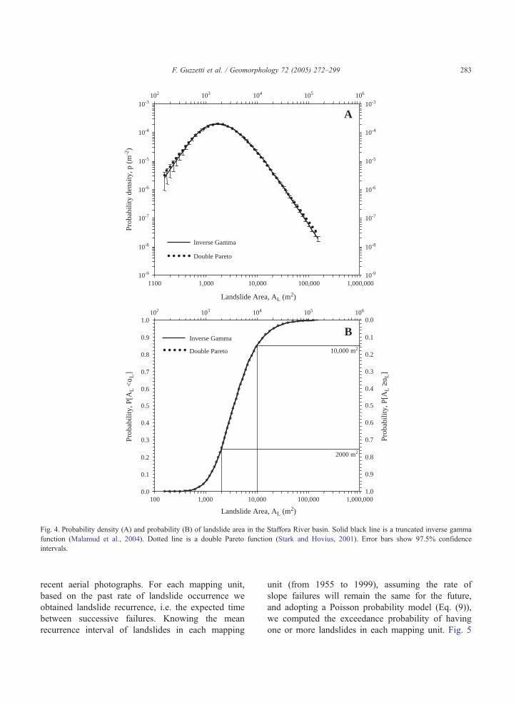
Fig. 4A shows the probability density function
(PDF) of landslide areas in the Staffora basin. Two
estimates of the PDF are shown. We obtained the first
estimate using the truncated inverse-gamma function
of Malamud et al. (2004) (Eq. (4)). For this estimate,
97.5% confidence intervals are also shown. We
obtained the second estimate using the double-Pareto
function of Stark and Hovius (2001) (Eq. (6)). In the
Landslide area
2 Total km2 Percentage* % Min m2 Mean m2 Max m2
34.72 49.30 57,300 390,100 2,384,900
38.24 54.30 900 27,900 826,700
2.46 3.49 700 8000 163,400
2.38 3.39 200 7500 51,000
4.41 6.26 100 6500 114,700
1.32 1.87 400 14,800 119,100
2.40 3.41 500 7900 119,100
2.06 2.92 500 4500 177,800
1.36 1.94 500 7800 77,900
0.65 0.93 3600 34,300 119,100
0.85 1.21 1900 22,400 119,100
63.22 90 900 41,300 2,384,900
70.42 100 100 17,900 2,384,900
46.43 66 100 12,100 177,800
12.08 17 100 3600 177,800
1.
area covered by landslides (A0–E2).
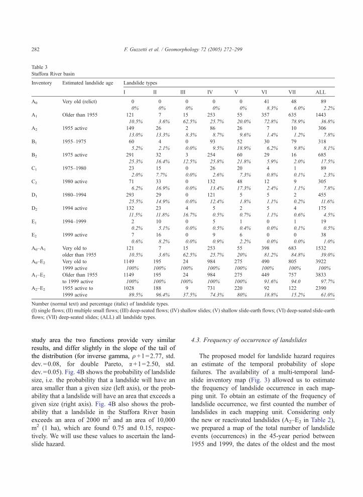
Table 3
Staffora River basin
Inventory Estimated landslide age Landslide types
I II III IV V VI VII ALL
A0 Very old (relict) 0 0 0 0 0 41 48 89
0% 0% 0% 0% 0% 8.3% 6.0% 2.2%
A1 Older than 1955 121 7 15 253 55 357 635 1443
10.5% 3.6% 62.5% 25.7% 20.0% 72.8% 78.9% 36.8%
A2 1955 active 149 26 2 86 26 7 10 306
13.0% 13.3% 8.3% 8.7% 9.6% 1.4% 1.2% 7.8%
B1 1955–1975 60 4 0 93 52 30 79 318
5.2% 2.1% 0.0% 9.5% 18.9% 6.2% 9.8% 8.1%
B2 1975 active 291 32 3 254 60 29 16 685
25.3% 16.4% 12.5% 25.8% 21.8% 5.9% 2.0% 17.5%
C1 1975–1980 23 15 0 26 20 4 1 89
2.0% 7.7% 0.0% 2.6% 7.3% 0.8% 0.1% 2.3%
C2 1980 active 71 33 0 132 48 12 9 305
6.2% 16.9% 0.0% 13.4% 17.3% 2.4% 1.1% 7.8%
D1 1980–1994 293 29 0 121 5 5 2 455
25.5% 14.9% 0.0% 12.4% 1.8% 1.1% 0.2% 11.6%
D2 1994 active 132 23 4 5 2 5 4 175
11.5% 11.8% 16.7% 0.5% 0.7% 1.1% 0.6% 4.5%
E1 1994–1999 2 10 0 5 1 0 1 19
0.2% 5.1% 0.0% 0.5% 0.4% 0.0% 0.1% 0.5%
E2 1999 active 7 16 0 9 6 0 0 38
0.6% 8.2% 0.0% 0.9% 2.2% 0.0% 0.0% 1.0%
A0–A1 Very old to
older than 1955
121 7 15 253 55 398 683 1532
10.5% 3.6% 62.5% 25.7% 20% 81.2% 84.8% 39.0%
A0–E2 Very old to
1999 active
1149 195 24 984 275 490 805 3922
100% 100% 100% 100% 100% 100% 100% 100%
A1–E2 Older than 1955
to 1999 active
1149 195 24 984 275 449 757 3833
100% 100% 100% 100% 100% 91.6% 94.0 97.7%
A2–E2 1955 active to
1999 active
1028 188 9 731 220 92 122 2390
89.5% 96.4% 37.5% 74.3% 80% 18.8% 15.2% 61.0%
Number (normal text) and percentage (italic) of landslide types.
(I) single flows; (II) multiple small flows; (III) deep-seated flows; (IV) shallow slides; (V) shallow slide-earth flows; (VI) deep-seated slide-earth
flows; (VII) deep-seated slides; (ALL) all landslide types.
F. Guzzetti et al. / Geomorphology 72 (2005) 272–299282
study area the two functions provide very similar
results, and differ slightly in the slope of the tail of
the distribution (for inverse gamma, q +1=2.77, std.
dev.=0.08, for double Pareto, a +1=2.50, std.
dev.=0.05). Fig. 4B shows the probability of landslide
size, i.e. the probability that a landslide will have an
area smaller than a given size (left axis), or the prob-
ability that a landslide will have an area that exceeds a
given size (right axis). Fig. 4B also shows the prob-
ability that a landslide in the Staffora River basin
exceeds an area of 2000 m2 and an area of 10,000
m2 (1 ha), which are found 0.75 and 0.15, respec-
tively. We will use these values to ascertain the land-
slide hazard.
4.3. Frequency of occurrence of landslides
The proposed model for landslide hazard requires
an estimate of the temporal probability of slope
failures. The availability of a multi-temporal land-
slide inventory map (Fig. 3) allowed us to estimate
the frequency of landslide occurrence in each map-
ping unit. To obtain an estimate of the frequency of
landslide occurrence, we first counted the number of
landslides in each mapping unit. Considering only
the new or reactivated landslides (A2–E2 in Table 2),
we prepared a map of the total number of landslide
events (occurrences) in the 45-year period between
1955 and 1999, the dates of the oldest and the most
Landslide Area, AL (m2)
Prob
abili
ty d
ensi
ty, p
(m
-2)
Double Pareto
Inverse Gamma
Landslide Area, AL (m2)
0.0
0.1
0.2
0.3
0.4
0.5
0.6
0.7
0.8
0.9
1.0
Prob
abili
ty, P
[AL <
L]
Double Pareto
Inverse Gamma
102 103 104 105 106
100 1,000 10,000 100,000 1,000,0001.0
0.9
0.8
0.7
0.6
0.5
0.4
0.3
0.2
0.1
0.0
Prob
abili
ty, P
[AL ≥
L]
10,000 m2
2000 m2
10-9
10-8
10-7
10-6
10-5
10-4
10-3
10-9
10-8
10-7
10-6
10-5
10-4
10-3
1100 1,000 10,000 100,000 1,000,000
102 103 104 105 106
A
B
a a
Fig. 4. Probability density (A) and probability (B) of landslide area in the Staffora River basin. Solid black line is a truncated inverse gamma
function (Malamud et al., 2004). Dotted line is a double Pareto function (Stark and Hovius, 2001). Error bars show 97.5% confidence
intervals.
F. Guzzetti et al. / Geomorphology 72 (2005) 272–299 283
recent aerial photographs. For each mapping unit,
based on the past rate of landslide occurrence we
obtained landslide recurrence, i.e. the expected time
between successive failures. Knowing the mean
recurrence interval of landslides in each mapping
unit (from 1955 to 1999), assuming the rate of
slope failures will remain the same for the future,
and adopting a Poisson probability model (Eq. (9)),
we computed the exceedance probability of having
one or more landslides in each mapping unit. Fig. 5
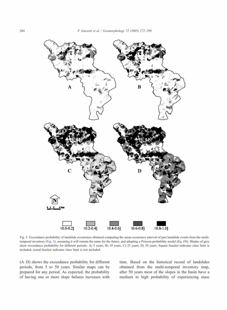
Fig. 5. Exceedance probability of landslide occurrence obtained computing the mean recurrence interval of past landslide events from the multi-
temporal inventory (Fig. 3), assuming it will remain the same for the future, and adopting a Poisson probability model (Eq. (9)). Shades of grey
show exceedance probability for different periods: A) 5 years, B) 10 years, C) 25 years, D) 50 years. Square bracket indicates class limit is
included; round bracket indicates class limit is not included.
F. Guzzetti et al. / Geomorphology 72 (2005) 272–299284
(A–D) shows the exceedance probability for different
periods, from 5 to 50 years. Similar maps can be
prepared for any period. As expected, the probability
of having one or more slope failures increases with
time. Based on the historical record of landslides
obtained from the multi-temporal inventory map,
after 50 years most of the slopes in the basin have a
medium to high probability of experiencing mass
A
0
5
10
15
20
25
30
35
1850
1860
1870
1880
1890
1900
1910
1920
1930
1940
1950
1960
1970
1980
1990
0
50
100
150
200
250
300
350
400
Num
ber
of la
ndsl
ides
Cum
ulat
ive
num
ber
of la
ndsl
ides
B
C
Recurrence from Inventory
Rec
urre
nce
from
Cat
alog
ue
0.0
0.1
0.2
0.3
0.4
0.5
0.6
0.7
0.0 0.1 0.2 0.3 0.4 0.5 0.6 0.7
N0 2 4 km 1
F. Guzzetti et al. / Geomorphology 72 (2005) 272–299 285
movements. We will use the obtained estimates to
ascertain landslide hazard.
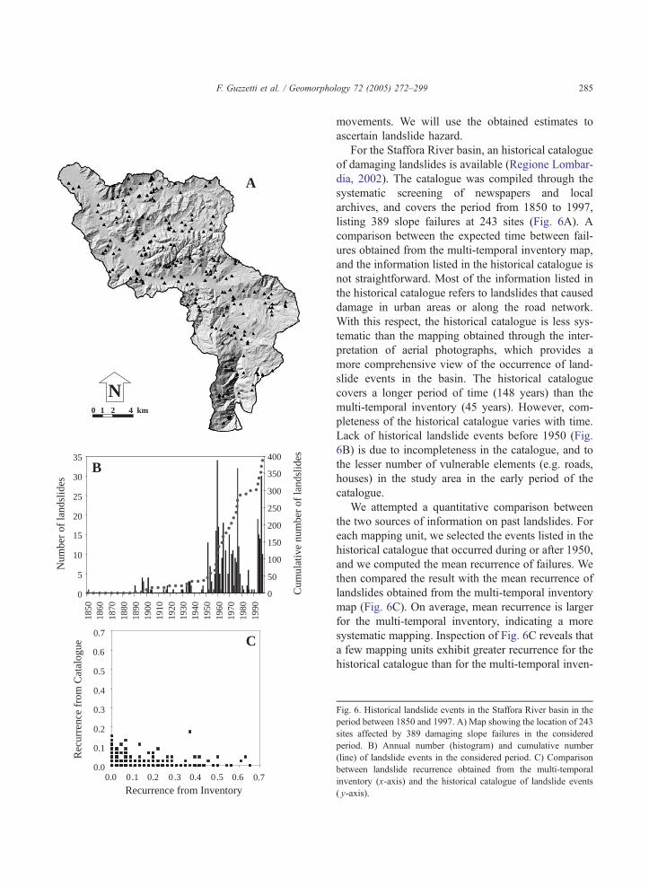
For the Staffora River basin, an historical catalogue
of damaging landslides is available (Regione Lombar-
dia, 2002). The catalogue was compiled through the
systematic screening of newspapers and local
archives, and covers the period from 1850 to 1997,
listing 389 slope failures at 243 sites (Fig. 6A). A
comparison between the expected time between fail-
ures obtained from the multi-temporal inventory map,
and the information listed in the historical catalogue is
not straightforward. Most of the information listed in
the historical catalogue refers to landslides that caused
damage in urban areas or along the road network.
With this respect, the historical catalogue is less sys-
tematic than the mapping obtained through the inter-
pretation of aerial photographs, which provides a
more comprehensive view of the occurrence of land-
slide events in the basin. The historical catalogue
covers a longer period of time (148 years) than the
multi-temporal inventory (45 years). However, com-
pleteness of the historical catalogue varies with time.
Lack of historical landslide events before 1950 (Fig.
6B) is due to incompleteness in the catalogue, and to
the lesser number of vulnerable elements (e.g. roads,
houses) in the study area in the early period of the
catalogue.
We attempted a quantitative comparison between
the two sources of information on past landslides. For
each mapping unit, we selected the events listed in the
historical catalogue that occurred during or after 1950,
and we computed the mean recurrence of failures. We
then compared the result with the mean recurrence of
landslides obtained from the multi-temporal inventory
map (Fig. 6C). On average, mean recurrence is larger
for the multi-temporal inventory, indicating a more
systematic mapping. Inspection of Fig. 6C reveals that
a few mapping units exhibit greater recurrence for the
historical catalogue than for the multi-temporal inven-
Fig. 6. Historical landslide events in the Staffora River basin in the
period between 1850 and 1997. A) Map showing the location of 243
sites affected by 389 damaging slope failures in the considered
period. B) Annual number (histogram) and cumulative numbe
(line) of landslide events in the considered period. C) Comparison
between landslide recurrence obtained from the multi-tempora
inventory (x-axis) and the historical catalogue of landslide events
( y-axis).
r
l
F. Guzzetti et al. / Geomorphology 72 (2005) 272–299286
tory map. Most of the slope failures listed in the
historical catalogue and located in these mapping
units (60%) occurred from 1956 to 1974, a period
for which aerial photographs were not available. Spe-
cific triggers (e.g., in 1959, 1960 and 1985) produced
many historical damaging landslides. For these trig-
gers, aerial photographs were also not available. In
addition, damaging slope failures in these mapping
units were small or very small, making their recogni-
tion on the aerial photographs very difficult.
4.4. Landslide susceptibility
The model for landslide hazard involves a quanti-
tative estimate of the probability of spatial landslide
occurrence, i.e. of susceptibility. We obtained land-
slide susceptibility through discriminant analysis of
46 thematic variables, including morphology (24 vari-
ables derived from a 20 m�20 m DTM), lithology
(14 variables), structure (3 variables) and land use (5
variables). Using GIS technology, we computed the
percentage of the individual thematic variables in each
mapping unit. The obtained values were the indepen-
dent variables in the statistical analysis. We then
computed the percentage of landslide area in each
mapping unit. Very old landslides (A0 in Table 2)
were excluded from the landslide inventory, and con-
sidered as a thematic variable, i.e., as an additional
independent variable describing the strength of the
lithological types. Following the procedure adopted
by Carrara et al. (1991), we selected a threshold of 3%
of landslide area to establish if a mapping unit was: (i)
free of landslides (V3%), or (ii) contained slope fail-
ures (N3%). We selected the threshold to account for
possible mapping, drafting and digitizing errors in the
compilation of the landslide inventory map (Carrara et
al., 1991).
Fig. 7 shows the results of five statistical models
prepared using the same set of environmental vari-
ables, and changing incrementally the landslide inven-
tory map. We prepared the first susceptibility model
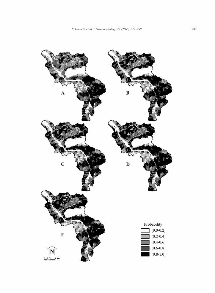
Fig. 7. Landslide susceptibility models obtained through discriminate anal
changing the landslide inventory map (dependent variable, Fig. 3 and Table
using landslides in the period A1–B2; C) using landslides in the period A1
the period A1–E2. Shades of gray indicate spatial probability, in 5 class
indicates class limit is not included.
(Fig. 7A) using only landslides identified in the 1955
photographs (Fig. 3A). These landslides included
recent (in 1955) and old landslides that were visible
in the aerial photographs used to compile the inven-
tory, but not the very old and relict landslides present
in the study area (A1–A2 in Table 2). We then added to
the inventory map the new landslides identified in the
1975 aerial photographs (Fig. 3B) and we obtained a
new estimate of the probability of spatial landslide
occurrence (Fig. 7B). We repeated the same procedure
adding the slope failures that we identified and
mapped using the 1980, 1994, and 1999 aerial photo-
graphs (Fig. 3C–E). Results are shown in Fig. 7C, D
and E, respectively. At each step, we obtained a
different susceptibility map, i.e. a different estimate
of the probability of spatial landslide occurrence.
Table 4 lists the variables entered into the five dis-
criminant models. In Table 4, the standard discrimi-
nant function coefficients (SDFC) show the relative
importance of each variable in the discriminant func-
tion as a predictor of slope instability. Variables with
large coefficients (in absolute value) are strongly
associated with the presence/absence of landslides.
The sign of the coefficient tells if the variable is
positively or negatively correlated to the stability of
the mapping unit.
Twenty-six of the 46 thematic variables (58%)
entered in all five susceptibility models, confirming
their importance in explaining the geographical distri-
bution of past landslides. Variables entered in all five
models include (Table 4) morphological (ORDER,
LINK_LEN, SLO_AREA, R, SLO_ANG, SLO_
ANG2, ANG_STD, LNK_ANG, CONV, COC_COV,
RET, CC, TR1), lithological (ALLUVIO, AR_
BIS, AR_R_M_P, DETRITO, MR_AN_LO, MR_
B_R_C, MR_BOSM, MR_P_R_B), and land use
(BD, BMD, INC, PRA, SEM, REG) parameters, and
the presence of very old, relict landslide deposits
(FRA_OLD). Inspection of Table 4 reveals that 8
thematic variables entered all five models with
large standard discriminant function coefficients
ysis of the same set of independent thematic variables (Table 4) and
2). A) Using landslides identified in the period A1–A2 (Table 2); B)
–C2; D) using landslides in the period A1–D2; E) using landslides in
es. Square bracket indicates class limit is included; round bracket
F. Guzzetti et al. / Geomorphology 72 (2005) 272–299 287
F. Guzzetti et al. / Geomorphology 72 (2005) 272–299288
(SDFCN |0.200|), equally distributed between nega-
tive (unstable) and positive (stable) values, including
the slope-unit hydrological order (ORDER), the
slope-unit gradient (SLO_ANG, SLO_ANG2), the
slope of the drainage channel (LNK_ANG), the topo-
graphic profile of the slope-unit (CC), the presence of
alluvial deposits (ALLUVIO) and of massive sand-
stone (AR_BIS), and the presence of uncultivated or
abandoned land (INC).
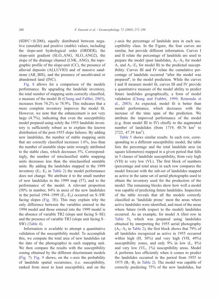
Fig. 8 allows for a comparison of the models
performance. By upgrading the landslide inventory,
the total number of mapping units correctly classified,
a measure of the model fit (Chung and Fabbri, 2003),
increases from 74.2% to 78.9%. This indicates that a
more complete inventory improves the model fit.
However, we note that the enhancement is not very
large (4.7%), indicating that even the susceptibility
model prepared using solely the 1955 landslide inven-
tory is sufficiently robust as to explain the known
distribution of the post-1955 slope failures. By adding
new landslides, the number of stable mapping units
that are correctly classified increases 1.6%, less than
the number of unstable slope units wrongly attributed
to the stable class, which decreases 5%. Correspond-
ingly, the number of misclassified stable mapping
units decreases less than the misclassified unstable
units. By adding the landslides mapped in the 1999
inventory (E1–E2 in Table 2) the model performance
does not change. We attribute it to the small number
of new landslides in the 1999 map (57), and to the
performance of the model. A relevant proportion
(50% in number, 84% in area) of the new landslides
in the period 1994–1999 (E1–E2) occurred on S–SW
facing slopes (Fig. 3E). This may explain why the
only difference between the variables entered in the
1994 model and those entered into the 1999 model is
the absence of variable TR2 (slope unit facing S–SE)
and the presence of variable TR3 (slope unit facing S–
SW) (Table 4).
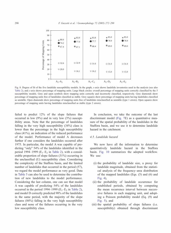
Information is available to attempt a quantitative
validation of the susceptibility model. To accomplish
this, we compute the total area of new landslides (at
the date of the photographs) in each mapping unit.
We then compare the results with the susceptibility
zoning obtained by the different discriminant models
(Fig. 7). Fig. 9 shows, on the x-axis the probability
of landslide spatial occurrence, (i.e. susceptibility,
ranked from most to least susceptible), and on the
y-axis the percentage of landslide area in each sus-
ceptibility class. In the Figure, the four curves are
similar, but provide different information. Curves I
and II relate the percentage of landslide are used to
prepare the model (past landslides, A1–A2 for model
A, and A1–E2 for model B) to the predicted suscept-
ibility. Curves III and IV relate the cumulative per-
centage of landslide occurred bafter the model was
preparedQ, to the model prediction. While the curves
I and II measure model fit, curves III and IV provide
a quantitative measure of the model ability to predict
future landslides geographically, a form of model
validation (Chung and Frabbri, 1999; Remondo et
al., 2003). As expected, model fit is better than
model performance, which decreases with the
increase of the time span of the prediction. We
attribute the improved performance of the model
(e.g. from model III to IV) chiefly to the augmented
number of landslides (from 1719, 40.76 km2 to
2722, 47.39 km2).
Table 5 shows similar results. In each row, corre-
sponding to a different susceptibility model, the table
lists the percentage and the total landslide area (in
square kilometres) mapped in a given period that falls
in 5 classes of landslide susceptibility, from very high
(VH) to very low (VL). The first block of numbers
(percentage and total area) in each row compares the
model forecast with the sub-set of landslides mapped
as active in the same set of aerial photographs used to
obtain the inventory used for the production of the
model. The remaining blocks show how well a model
was capable of predicting future landslides. Inspection
of the table reveals that all the models correctly
classified as dlandslide proneT most the areas where
active landslides were identified, and most of the areas
where future (with respect to the model) landslides
occurred. As an example, for model A (first row in
Table 5), which was prepared using landslides
obtained by interpreting the 1955 aerial photography
(A1–A2 in Table 2), the first block shows that 79% of
all landslides recognized as active in 1955 occurred
within high (H, 30%) and very high (VH, 49%)
susceptibility zones, and only 9% in low (L, 8%)
and very low (VL, 1%) susceptibility areas. Model
A performs less efficiently when it comes to predict
the landslides occurred in the period from 1955 to
1975 (B1–B2 in Table 2). The model was capable of
correctly predicting 75% of the new landslides, but
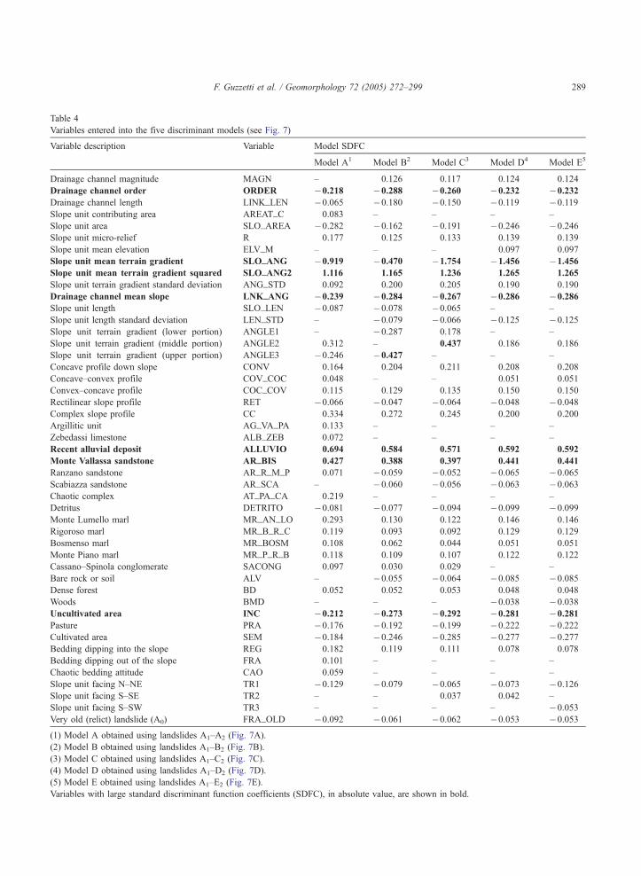
Table 4
Variables entered into the five discriminant models (see Fig. 7)
Variable description Variable Model SDFC
Model A1 Model B2 Model C3 Model D4 Model E5
Drainage channel magnitude MAGN – 0.126 0.117 0.124 0.124
Drainage channel order ORDER 0.218 0.288 0.260 0.232 0.232
Drainage channel length LINK_LEN 0.065 0.180 0.150 0.119 0.119
Slope unit contributing area AREAT_C 0.083 – – – –
Slope unit area SLO_AREA 0.282 0.162 0.191 0.246 0.246
Slope unit micro-relief R 0.177 0.125 0.133 0.139 0.139
Slope unit mean elevation ELV_M – – – 0.097 0.097
Slope unit mean terrain gradient SLO_ANG 0.919 0.470 1.754 1.456 1.456
Slope unit mean terrain gradient squared SLO_ANG2 1.116 1.165 1.236 1.265 1.265
Slope unit terrain gradient standard deviation ANG_STD 0.092 0.200 0.205 0.190 0.190
Drainage channel mean slope LNK_ANG 0.239 0.284 0.267 0.286 0.286
Slope unit length SLO_LEN 0.087 0.078 0.065 – –
Slope unit length standard deviation LEN_STD – 0.079 0.066 0.125 0.125
Slope unit terrain gradient (lower portion) ANGLE1 – 0.287 0.178 – –
Slope unit terrain gradient (middle portion) ANGLE2 0.312 – 0.437 0.186 0.186
Slope unit terrain gradient (upper portion) ANGLE3 0.246 0.427 – – –
Concave profile down slope CONV 0.164 0.204 0.211 0.208 0.208
Concave–convex profile COV_COC 0.048 – – 0.051 0.051
Convex–concave profile COC_COV 0.115 0.129 0.135 0.150 0.150
Rectilinear slope profile RET 0.066 0.047 0.064 0.048 0.048
Complex slope profile CC 0.334 0.272 0.245 0.200 0.200
Argillitic unit AG_VA_PA 0.133 – – – –
Zebedassi limestone ALB_ZEB 0.072 – – – –
Recent alluvial deposit ALLUVIO 0.694 0.584 0.571 0.592 0.592
Monte Vallassa sandstone AR_BIS 0.427 0.388 0.397 0.441 0.441
Ranzano sandstone AR_R_M_P 0.071 0.059 0.052 0.065 0.065
Scabiazza sandstone AR_SCA – 0.060 0.056 0.063 0.063
Chaotic complex AT_PA_CA 0.219 – – – –
Detritus DETRITO 0.081 0.077 0.094 0.099 0.099
Monte Lumello marl MR_AN_LO 0.293 0.130 0.122 0.146 0.146
Rigoroso marl MR_B_R_C 0.119 0.093 0.092 0.129 0.129
Bosmenso marl MR_BOSM 0.108 0.062 0.044 0.051 0.051
Monte Piano marl MR_P_R_B 0.118 0.109 0.107 0.122 0.122
Cassano–Spinola conglomerate SACONG 0.097 0.030 0.029 – –
Bare rock or soil ALV – 0.055 0.064 0.085 0.085
Dense forest BD 0.052 0.052 0.053 0.048 0.048
Woods BMD – – – 0.038 0.038
Uncultivated area INC 0.212 0.273 0.292 0.281 0.281
Pasture PRA 0.176 0.192 0.199 0.222 0.222
Cultivated area SEM 0.184 0.246 0.285 0.277 0.277
Bedding dipping into the slope REG 0.182 0.119 0.111 0.078 0.078
Bedding dipping out of the slope FRA 0.101 – – – –
Chaotic bedding attitude CAO 0.059 – – – –
Slope unit facing N–NE TR1 0.129 0.079 0.065 0.073 0.126
Slope unit facing S–SE TR2 – – 0.037 0.042 –
Slope unit facing S–SW TR3 – – – – 0.053
Very old (relict) landslide (A0) FRA_OLD 0.092 0.061 0.062 0.053 0.053
(1) Model A obtained using landslides A1–A2 (Fig. 7A).
(2) Model B obtained using landslides A1–B2 (Fig. 7B).
(3) Model C obtained using landslides A1–C2 (Fig. 7C).
(4) Model D obtained using landslides A1–D2 (Fig. 7D).
(5) Model E obtained using landslides A1–E2 (Fig. 7E).
Variables with large standard discriminant function coefficients (SDFC), in absolute value, are shown in bold.
F. Guzzetti et al. / Geomorphology 72 (2005) 272–299 289
80.083.9 83.8 85.0 85.0
74.277.0 77.7 78.9 78.9
67.4 67.1 68.4 69.0 69.0
20.016.1 16.2 15.0 15.0
32.6 32.9 31.6 31.0 31.0
0
10
20
30
40
50
60
70
80
90
100
Perc
enta
ge o
f M
appi
ng U
nits
A1–A2 A1–B2 A1–C2 A1–D2 A1–E2
Fig. 8. Degree of fit of the five landslide susceptibility models. In the graph, x-axis shows landslide inventories used in the analysis (see also
Table 2), and y-axis shows percentage of mapping units. Large black circles: overall percentage of mapping units correctly classified by the 5
susceptibility models. Grey and open symbols show mapping units correctly and incorrectly classified, respectively. Grey diamonds show
percentage of mapping units free of landslides classified as stable. Grey squares show percentage of mapping units having landslides classified
as unstable. Open diamonds show percentage of mapping units free of landslides misclassified as unstable (type 1 errors). Open squares show
percentage of mapping units having landslides misclassified as stable (type 2 errors).
F. Guzzetti et al. / Geomorphology 72 (2005) 272–299290
failed to predict 12% of the slope failures that
occurred in low (9%) and in very low (3%) suscept-
ibility areas. Note that the percentage of landslides
falling in the very high susceptibility (34%) class is
lower than the percentage in the high susceptibility
class (41%), an indication of the reduced performance
of the model. Performance of model A decreases
further if one considers the landslides occurred after
1975. In particular, the model A was capable of pre-
dicting bonlyQ 54% of the landslides identified in the
period 1994–1999 (E1–E2 in Table 2), with a consid-
erable proportion of slope failures (31%) occurring in
the unclassified (U) susceptibility class. Considering
the complexity of the Staffora basin, and the limited
number of landslides that occurred in the period (57),
we regard the model performance as very good. Data
in Table 5 can also be used to determine the contribu-
tion of new landslides to the model performance.
Considering the last column, one can see that model
A was capable of predicting 54% of the landslides
occurred in the period 1994–1999 (E1–E2 in Table 2),
and model D correctly predicted 98% of the landslides
in the same period, with the majority of the slope
failures (84%) falling in the very high susceptibility
class and none of the failures occurring in the very
low susceptibility class.
In conclusion, we take the outcome of the last
discriminant model (Fig. 7E) as a quantitative mea-
sure of the spatial probability of the landslides in the
Staffora basin, and we use it to determine landslide
hazard in the catchment.
4.5. Landslide hazard
We now have all the information to determine
quantitatively landslide hazard in the Staffora
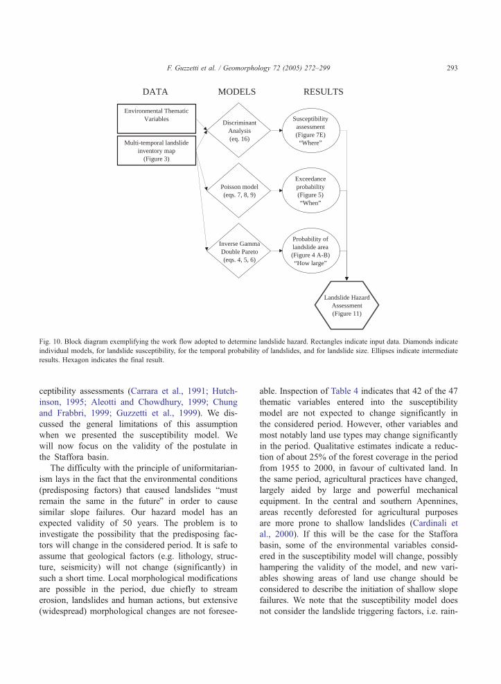
basin. Fig. 10 summarizes the adopted workflow.
We use:
(i) the probability of landslide size, a proxy for
landslide magnitude, obtained from the statisti-
cal analysis of the frequency–area distribution
of the mapped landslides (Eqs. (5) and (6) and
Fig. 4),
(ii) the probability of landslide occurrence for
established periods, obtained by computing
the mean recurrence interval between succes-
sive failures in each mapping unit, and adopt-
ing a Poisson probability model (Eq. (9) and
Fig. 5), and
(iii) the spatial probability of slope failures (i.e.
susceptibility) obtained through discriminant
0
10
20
30
40
50
60
70
80
90
100
0 10 20 30 40 50 60 70 80 90 100
I
II
III
IV
Percentage of study area in the susceptibility classes
Perc
enta
ge o
f la
ndsl
ide
area
in th
e su
scep
tibili
ty c
lass
es
most susceptible least susceptible
Fig. 9. Graph comparing model fit and model performance (prediction rate). In the graph, the x-axis shows the probability of landslide spatial
occurrence (susceptibility), ranked from most (left) to least (right) susceptible, and y-axis shows the percentage of landslide area in each
susceptibility class. Curve I and II illustrate model fit. Curve I shows the ability of the model obtained using landslides identified in the period
A1–A2 (Table 2) to forecast the same set of landslides. Curve II shows the capacity of the model prepared using landslides in the period A1–E2 to
forecast recent landslides identified in the 1999 aerial photographs (E1–E2). Curve III and IV illustrate model performance. Curve III indicates
the ability of the model prepared using landslides identified in the period A1–A2 to forecast bfutureQ landslides occurred in the period B1–E2.
Curve IV indicates the ability of the model prepared using landslides identified in the period A1–B2 to forecast bfutureQ landslides occurred in
the period C1–E2.
F. Guzzetti et al. / Geomorphology 72 (2005) 272–299 291
analysis of 46 environmental variables (Eq. (13)
and Fig. 7).
Assuming independence (Eq. (2)), we multiply the
three probabilities and we obtain landslide hazard, i.e.
the joint probability that a mapping unit will be
affected by future landslides that exceed a given
size, in a given time, and because of the local envir-
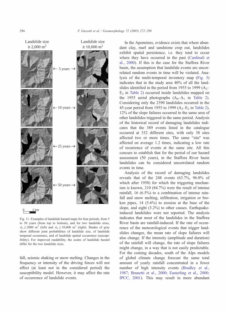
onmental setting. Fig. 11 shows examples of the land-
slide hazard assessment. The figure portrays landslide
hazard for mapping units in the central part of the
Staffora river basin, for four periods (5, 10, 25 and 50
years), and for two different landslide sizes, greater or
equal than 2000 m2, and greater or equal than 10,000
m2 (1 ha).
5. Discussion of the results
The proposed method allowed us to determine
quantitatively landslide hazard in the Staffora River
basin. We obtained most of the information used in
the analysis from a detailed multi-temporal inven-
tory map. Production of the multi-temporal in-
ventory required a total of 6 months of three
geomorphologists. Digitization and validation of
the map required a total of one month of two GIS
experts. Statistical analysis and hazard modelling
required three weeks of two geomorphologists. Con-
sidering the thematic information used to ascertain
susceptibility (i.e., DTM, geology, land use) was
already available in digital format (Antonini et al.,
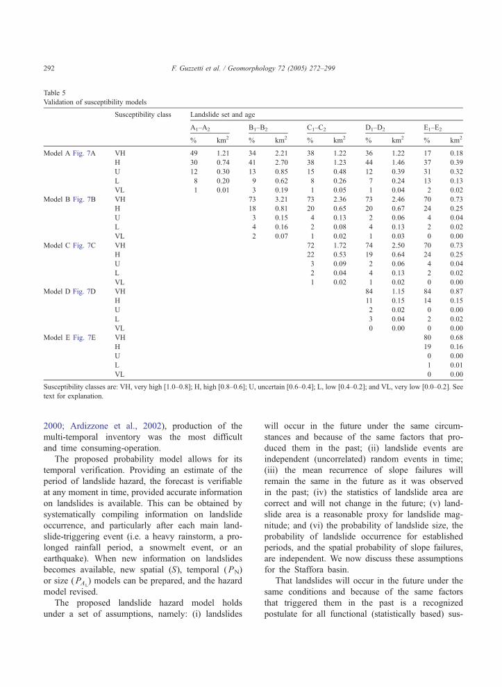
Table 5
Validation of susceptibility models
Susceptibility class Landslide set and age
A1–A2 B1–B2 C1–C2 D1–D2 E1–E2
% km2 % km2 % km2 % km2 % km2
Model A Fig. 7A VH 49 1.21 34 2.21 38 1.22 36 1.22 17 0.18
H 30 0.74 41 2.70 38 1.23 44 1.46 37 0.39
U 12 0.30 13 0.85 15 0.48 12 0.39 31 0.32
L 8 0.20 9 0.62 8 0.26 7 0.24 13 0.13
VL 1 0.01 3 0.19 1 0.05 1 0.04 2 0.02
Model B Fig. 7B VH 73 3.21 73 2.36 73 2.46 70 0.73
H 18 0.81 20 0.65 20 0.67 24 0.25
U 3 0.15 4 0.13 2 0.06 4 0.04
L 4 0.16 2 0.08 4 0.13 2 0.02
VL 2 0.07 1 0.02 1 0.03 0 0.00
Model C Fig. 7C VH 72 1.72 74 2.50 70 0.73
H 22 0.53 19 0.64 24 0.25
U 3 0.09 2 0.06 4 0.04
L 2 0.04 4 0.13 2 0.02
VL 1 0.02 1 0.02 0 0.00
Model D Fig. 7D VH 84 1.15 84 0.87
H 11 0.15 14 0.15
U 2 0.02 0 0.00
L 3 0.04 2 0.02
VL 0 0.00 0 0.00
Model E Fig. 7E VH 80 0.68
H 19 0.16
U 0 0.00
L 1 0.01
VL 0 0.00
Susceptibility classes are: VH, very high [1.0–0.8]; H, high [0.8–0.6]; U, uncertain [0.6–0.4]; L, low [0.4–0.2]; and VL, very low [0.0–0.2]. See
text for explanation.
F. Guzzetti et al. / Geomorphology 72 (2005) 272–299292
2000; Ardizzone et al., 2002), production of the
multi-temporal inventory was the most difficult
and time consuming-operation.
The proposed probability model allows for its
temporal verification. Providing an estimate of the
period of landslide hazard, the forecast is verifiable
at any moment in time, provided accurate information
on landslides is available. This can be obtained by
systematically compiling information on landslide
occurrence, and particularly after each main land-
slide-triggering event (i.e. a heavy rainstorm, a pro-
longed rainfall period, a snowmelt event, or an
earthquake). When new information on landslides
becomes available, new spatial (S), temporal (PN)
or size (PAL) models can be prepared, and the hazard
model revised.
The proposed landslide hazard model holds
under a set of assumptions, namely: (i) landslides
will occur in the future under the same circum-
stances and because of the same factors that pro-
duced them in the past; (ii) landslide events are
independent (uncorrelated) random events in time;
(iii) the mean recurrence of slope failures will
remain the same in the future as it was observed
in the past; (iv) the statistics of landslide area are
correct and will not change in the future; (v) land-
slide area is a reasonable proxy for landslide mag-
nitude; and (vi) the probability of landslide size, the
probability of landslide occurrence for established
periods, and the spatial probability of slope failures,
are independent. We now discuss these assumptions
for the Staffora basin.
That landslides will occur in the future under the
same conditions and because of the same factors
that triggered them in the past is a recognized
postulate for all functional (statistically based) sus-
Environmental ThematicVariables
Multi-temporal landslideinventory map
(Figure 3)
Susceptibilityassessment(Figure 7E)
“Where”
DiscriminantAnalysis(eq. 16)
Exceedanceprobability(Figure 5)“When”
Poisson model(eqs. 7, 8, 9)
Probability oflandslide area(Figure 4 A-B)“How large”
Inverse GammaDouble Pareto(eqs. 4, 5, 6)
DATA MODELS RESULTS
Landslide HazardAssessment(Figure 11)
Fig. 10. Block diagram exemplifying the work flow adopted to determine landslide hazard. Rectangles indicate input data. Diamonds indicate
individual models, for landslide susceptibility, for the temporal probability of landslides, and for landslide size. Ellipses indicate intermediate
results. Hexagon indicates the final result.
F. Guzzetti et al. / Geomorphology 72 (2005) 272–299 293
ceptibility assessments (Carrara et al., 1991; Hutch-
inson, 1995; Aleotti and Chowdhury, 1999; Chung
and Frabbri, 1999; Guzzetti et al., 1999). We dis-
cussed the general limitations of this assumption
when we presented the susceptibility model. We
will now focus on the validity of the postulate in
the Staffora basin.
The difficulty with the principle of uniformitarian-
ism lays in the fact that the environmental conditions
(predisposing factors) that caused landslides bmust
remain the same in the futureQ in order to cause
similar slope failures. Our hazard model has an
expected validity of 50 years. The problem is to
investigate the possibility that the predisposing fac-
tors will change in the considered period. It is safe to
assume that geological factors (e.g. lithology, struc-
ture, seismicity) will not change (significantly) in
such a short time. Local morphological modifications
are possible in the period, due chiefly to stream
erosion, landslides and human actions, but extensive
(widespread) morphological changes are not foresee-
able. Inspection of Table 4 indicates that 42 of the 47
thematic variables entered into the susceptibility
model are not expected to change significantly in
the considered period. However, other variables and
most notably land use types may change significantly
in the period. Qualitative estimates indicate a reduc-
tion of about 25% of the forest coverage in the period
from 1955 to 2000, in favour of cultivated land. In
the same period, agricultural practices have changed,
largely aided by large and powerful mechanical
equipment. In the central and southern Apennines,
areas recently deforested for agricultural purposes
are more prone to shallow landslides (Cardinali et
al., 2000). If this will be the case for the Staffora
basin, some of the environmental variables consid-
ered in the susceptibility model will change, possibly
hampering the validity of the model, and new vari-
ables showing areas of land use change should be
considered to describe the initiation of shallow slope
failures. We note that the susceptibility model does
not consider the landslide triggering factors, i.e. rain-
5 years
0 1 km
Landslide size≥ 2,000 m2
Landslide size≥ 10,000 m2
10 years
25 years
50 years
Fig. 11. Examples of landslide hazard maps for four periods, from 5
to 50 years (from top to bottom), and for two landslide sizes,
ALz2000 m2 (left) and ALz10,000 m2 (right). Shades of gray
show different joint probabilities of landslide size, of landslide
temporal occurrence, and of landslide spatial occurrence (suscept-
ibility). For improved readability, the scales of landslide hazard
differ for the two landslide sizes.
F. Guzzetti et al. / Geomorphology 72 (2005) 272–299294
fall, seismic shaking or snow melting. Changes in the
frequency or intensity of the driving forces will not
affect (at least not in the considered period) the
susceptibility model. However, it may affect the rate
of occurrence of landslide events.
In the Apennines, evidence exists that where abun-
dant clay, marl and sandstone crop out, landslides
exhibit spatial persistence, i.e. they tend to occur
where they have occurred in the past (Cardinali et
al., 2000). If this is the case for the Staffora River
basin, the assumption that landslide events are uncor-
related random events in time will be violated. Ana-
lysis of the multi-temporal inventory map (Fig. 3)
indicates that in the study area 40% of all the land-
slides identified in the period from 1955 to 1999 (A2–
E2 in Table 2) occurred inside landslides mapped on
the 1955 aerial photographs (A0–A1 in Table 2).
Considering only the 2390 landslides occurred in the
45-year period from 1955 to 1999 (A2–E2 in Table 2),
12% of the slope failures occurred in the same area of
other landslides triggered in the same period. Analysis
of the historical record of damaging landslides indi-
cates that the 389 events listed in the catalogue
occurred at 332 different sites, with only 38 sites
affected two or more times. The same bsiteQ was
affected on average 1.2 times, indicating a low rate
of recurrence of events at the same site. All this
concurs to establish that for the period of our hazard
assessment (50 years), in the Staffora River basin
landslides can be considered uncorrelated random
events in time.
Analysis of the record of damaging landslides
reveals that of the 248 events (63.7%, 96.0% of
which after 1950) for which the triggering mechan-
ism is known, 210 (84.7%) were the result of intense
rainfall, 16 (6.5%) to a combination of intense rain-
fall and snow melting, infiltration, irrigation or bro-
ken pipes, 14 (5.6%) to erosion at the base of the
slope, and eight (3.2%) to other causes. Earthquake-
induced landslides were not reported. The analysis
indicates that most of the landslides in the Staffora
River basin are rainfall-induced. If the rate of occur-
rence of the meteorological events that trigger land-
slides changes, the mean rate of slope failures will
also change. If the intensity (amplitude and duration)
of the rainfall will change, the rate of slope failures
might change, in a way that is not easily predictable.
For the coming decades, south of the Alps models
of global climate change forecast the same total
amount of yearly rainfall concentrated in a fewer
number of high intensity events (Bradley et al.,
1987; Brunetti et al., 2000; Easterling et al., 2000;
IPCC, 2001). This may result in more abundant
F. Guzzetti et al. / Geomorphology 72 (2005) 272–299 295
shallow landslides, and in less frequent deep-seated
slope failures (Buma and Dehn, 1998; Malet et al.,
2005). Modifications in land use induced by changes
in agricultural practices may also change the rate of
occurrence of landslides.
Determining the statistics of landslide areas is no
trivial task (Malamud et al., 2004). Only a handful of
inventories are available which are substantially
complete and have enough cartographic detail to
allow for determining unambiguously the PDF of
landslide areas (Stark and Hovius, 2001; Guzzetti
et al., 2002a,b; Guthrie and Evans, 2004a,b; Mala-
mud et al., 2004). The (scant) available information
indicates that the frequency–area statistics of land-
slide areas does not change significantly across litho-
logical or physiographical boundaries. Malamud et
al. (2004) showed that three different populations of
landslides produced by different triggers (i.e. seismic
shaking, intense rainfall, rapid snow melting) in
different physiographical regions (southern Califor-
nia, central America, central Italy), exhibit virtually
identical PDFs. Unpublished work conducted in cen-
tral Italy indicates that for the same physiographical
region the PDF of landslide area does not change in
time. It is, therefore, safe to assume that in the
Staffora River basin the frequency–area statistics of
landslide area will not change in the period of the
hazard assessment. It is also justified to use a single
PDF for the entire basin. Since the most abundant
landslides in the catchment are small (~2000 m2, Fig.
4A), great care must be taken in mapping accurately
(and completely) the small slope failures. The slope
of the heavy tail of the PDF in Fig. 4A is controlled
by a limited number of landslides. There are 16
landslides larger than 50,000 m2 (5 ha) and only
one landslide larger than 100,000 m2 (10 ha). Care
must be taken in mapping the largest landslides, and
in deciding whether they represent an individual
slope failure or the result of two or more coalescent
landslides.
Hungr (1997) argued that no unique measure of
landslide magnitude is available, and proposed to
adopt destructiveness as measure of landslide mag-
nitude. In this work, we have taken landslide area as
a proxy for landslide destructiveness (and of land-
slide magnitude). We obtained the area of the in-
dividual slope failures from the multi-temporal
landslide inventory in GIS format. However, is land-
slide area a good measure of landslide destructiveness
in the Staffora basin? Analysis of the historical cat-
alogue of damaging slope failures reveals that infor-
mation on the size (area, length and width) of
landslides is available for 26 events (6.7%), which
range from 600 m2 to 600,000 m2 (mean=58,000 m2,
std. dev.=13,500 m2). Damage caused by these land-
slides was mostly to the road network and, sub-
ordinately, to private homes and to the aqueduct.
Casualties were not reported. Information on the land-
slide type is available for 28 events (7.2%), of which
15 were slides, 6 flows and 5 falls. Slides and flows
caused the most severe damage, and falls produced
only minor interruptions along the roads. Information
on landslide velocity is available for five events, and
ranges from 1.2�101 to 5.8�103 mm/s (moderate
landslide velocity (Cruden and Varnes, 1996)). As a
whole, the available historical information on dama-
ging slope failures suggests that: (i) damage in the
Staffora River basin is caused mostly by slow to
rapid moving slides and flows, i.e. the type of failures
considered in the hazard assessment, and (ii) large
landslides tend to produce larger damage, particularly
to roads.
The last assumption of the proposed model is that
the probabilities of landslide size, of temporal occur-
rence, and of spatial incidence of mass movements are
independent. The legitimacy of this assumption is
difficult to prove quantitatively. We have shown that
the probability of landslide area is largely independent
from the physiographical setting. As a first-approxi-
mation, it is safe to conclude that the probability of
landslide area is independent from susceptibility. The
susceptibility model was constructed without consid-
ering the driving forces (meteorological or else) that
control the rate of occurrence of slope failures in the
Staffora River basin. We conclude that the rate of
landslide events is independent from susceptibility.
The catalogue of historical damaging landslides
reveals that landslides occurred in all sizes. We con-
sider this an indication that the rate of failures is
independent from landslide size.
Finally, the main scope of a landslide hazard
assessment is to provide quantitative expertise on
future slope failures to planners, decision-makers,
civil defence authorities, insurance companies, land
developers, and individual landowners. The pro-
posed method allowed us to prepare a large number
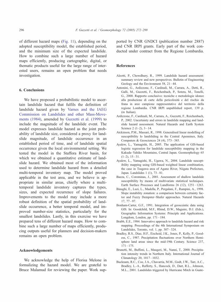
F. Guzzetti et al. / Geomorphology 72 (2005) 272–299296
of different hazard maps (Fig. 11), depending on the
adopted susceptibility model, the established period,
and the minimum size of the expected landslide.
How to combine such a large number of hazard
maps efficiently, producing cartographic, digital, or
thematic products useful for the large range of inter-
ested users, remains an open problem that needs
investigation.
6. Conclusions
We have proposed a probabilistic model to ascer-
tain landslide hazard that fulfils the definition of
landslide hazard given by Varnes and the IAEG
Commission on Landslides and other Mass-Move-
ments (1984), amended by Guzzetti et al. (1999) to
include the magnitude of the landslide event. The
model expresses landslide hazard as the joint prob-
ability of landslide size, considered a proxy for land-
slide magnitude, of landslide occurrence in an
established period of time, and of landslide spatial
occurrence given the local environmental setting. We
tested the model in the Staffora River basin, for
which we obtained a quantitative estimate of land-
slide hazard. We obtained most of the information
used to determine landslide hazard from a detailed
multi-temporal inventory map. The model proved
applicable in the test area, and we believe is ap-
propriate in similar areas, chiefly where a multi-
temporal landslide inventory captures the types,
sizes, and expected recurrence of slope failures.
Improvements to the model may include a more
robust definition of the spatial probability of land-
slide occurrence, a better temporal model, and im-
proved number-size statistics, particularly for the
smallest landslides. Lastly, in this exercise we have
prepared tens of different hazard maps. How to com-
bine such a large number of maps efficiently, produ-
cing outputs useful for planners and decision-makers
remains an open problem.
Acknowledgements
We acknowledge the help of Florisa Melone in
formalizing the hazard model. We are grateful to
Bruce Malamud for reviewing the paper. Work sup-
ported by CNR GNDCI (publication number 2887)
and CNR IRPI grants. Early part of the work con-
ducted under contract from the Regione Lombardia.
References
Aleotti, P., Chowdhury, R., 1999. Landslide hazard assessment:
summary review and new perspectives. Bulletin of Engineering
Geology and the Environment 58, 21–44.
Antonini, G., Ardizzone, F., Cardinali, M., Carrara, A., Detti, R.,
Galli, M., Guzzetti, F., Reichenbach, P., Sotera, M., Tonelli,
G., 2000. Rapporto conclusivo: tecniche e metodologie idonee
alla produzione di carte della pericolosita e del rischio da
frana in aree campione rappresentative del territorio della
regione Lombardia. CNR IRPI unpublished report, 139 p.
(in Italian).
Ardizzone, F., Cardinali, M., Carrara, A., Guzzetti, F., Reichenbach,
P., 2002. Uncertainty and errors in landslide mapping and land-
slide hazard assessment. Natural Hazards and Earth System
Science 2 (1–2), 3–14.
Atckinson, P.M., Massari, R., 1998. Generalised linear modelling of
susceptibility lo landsliding in the Central Apennines, Italy.
Computers & Geosciences 24 (4), 373–385.
Ayalew, L., Yamagishi, H., 2005. The application of GIS-based
logistic regression for landslide susceptibility mapping in the
Kakuda–Yahiko Mountains, Central Japan. Geomorphology 65
(1–2), 15–31.
Ayalew, L., Yamagishi, H., Ugawa, N., 2004. Landslide suscept-
ibility mapping using GIS-based weighted linear combination,
the case in Tsugawa area of Agano River, Niigata Prefecture,
Japan. Landslides 1 (1), 73–81.
Baeza, C., Corominas, J., 2001. Assessment of shallow landslide
susceptibility by means of multivariate statistical techniques.
Earth Surface Processes and Landforms 26 (12), 1251–1263.
Binaghi, E., Luzi, L., Madella, P., Pergalani, F., Rampini, A., 1998.
Slope instability zonation: a comparison between certainty fac-
tor and Fuzzy Dempster–Shafer approaches. Natural Hazards
17, 77–97.
Bonham-Carter, G.F., 1991. Integration of geosceintic data using
GIS. In: Goodchild, M.F., Rhind, D.W., Maguire, D.J. (Eds.),
Geographic Information Systems: Principle and Applications.
Longdom, London, pp. 171–184.
Brabb, E.E., 1984. Innovative approach to landslide hazard and risk
mapping. Proceedings of the 4th International Symposium on
Landslides, Toronto, vol. 1, pp. 307–324.
Bradley, R.S., Diaz, H.F., Eischeid, J.K., Jones, P., Kelly, P., Good-
ess, C., 1987. Precipitation fluctuations over Northern Hemi-
sphere land areas since the mid-19th Century. Science 237,
171–175.
Brunetti, M., Buffoni, L., Maugeri, M., Nanni, T., 2000. Precipita-
tion intensity trends in Northern Italy. International Journal of
Climatology 20, 1017–1032.
Bucknam, R.C., Coe, J.A., Chavarria, M.M., Godt, J.W., Tarr, A.C.,
Bradley, L.-A., Rafferty, S., Hancock, D., Dart, R.L., Johnson,
M.L., 2001. Landslides triggered by Hurricane Mitch in Guate-
F. Guzzetti et al. / Geomorphology 72 (2005) 272–299 297
mala — inventory and discussion. U.S. Geological Survey Open
File Report 01-443 (38 pp.).
Buma, J., Dehn, M., 1998. A method for predicting the impact of
climate change on slope stability. Environmental Geology 35
(2–3), 190–196.
Cardinali, M., Ardizzone, F., Galli, M., Guzzetti, F., Reichenbach,
P., 2000. Landslides triggered by rapid snow melting: the
December 1996–January 1997 event in Central Italy. In:
Claps, P., Siccardi, F. (Eds.), Proceedings 1st Plinius Con-
ference on Mediterranean Storms. Bios Publisher, Cosenza,
pp. 439–448.
Cardinali, M., Carrara, A., Guzzetti, F., Reichenbach, P., 2002a.
Landslide hazard map for the Upper Tiber River basin.
CNR GNDCI Publication number 2116, map at 1 :100,000
scale.
Cardinali, M., Reichenbach, P., Guzzetti, F., Ardizzone, F.,
Antonini, G., Galli, M., Cacciano, M., Castellani, M., Sal-
vati, P., 2002b. A geomorphological approach to estimate
landslide hazard and risk in urban and rural areas in Umbria,
central Italy. Natural Hazards and Earth System Science 2
(1–2), 57–72.
Carrara, A., 1983. A multivariate model for landslide hazard eva-
luation. Mathematical Geology 15, 403–426.
Carrara, A., Cardinali, M., Detti, R., Guzzetti, F., Pasqui, V., Reich-
enbach, P., 1991. GIS techniques and statistical models in
evaluating landslide hazard. Earth Surface Processes and Land-
form 16 (5), 427–445.
Carrara, A., Cardinali, M., Guzzetti, F., 1992. Uncertainty in asses-
sing landslide hazard and risk. ITC Journal 2, 172–183.
Carrara, A., Cardinali, M., Guzzetti, F., Reichenbach, P., 1995. GIS
technology in mapping landslide hazard. In: Carrara, A., Guz-
zetti, F. (Eds.), Geographical Information Systems in Assessing
Natural Hazards. Kluwer Academic Publisher, Dordrecht, The
Netherlands, pp. 135–175.
Carrara, A., Crosta, G.B., Frattini, P., 2003. Geomorphological and
historical data in assessing landslide hazard. Earth Surface
Processes and Landforms 28 (10), 1125–1142.
Cevik, E., Topal, T., 2003. GIS-based landslide susceptibility map-
ping for a problematic segment of the natural gas pipeline,
Hendek (Turkey). Environmental Geology 44 (8), 949–962.
Chung, C.J., Frabbri, A.G., 1999. Probabilistic prediction models
for landslide hazard mapping. Photogrammetric Engineering
and Remote Sensing 65 (12), 1389–1399.
Chung, C.J., Fabbri, A.G., 2003. Validation of spatial prediction
models for landslide hazard mapping. Natural Hazards 30 (3),
451–472.
Chung, C.J., Fabbri, A.G., 2005. Systematic procedures of landslide
hazard mapping for risk assessment using spatial prediction
models. In: Glade, C.J., et al., (Eds.), Landslide Risk Assess-
ment. John Wiley, pp. 139–174.
Coe, J.A., Michael, J.A., Crovelli, R.A., Savage, W.Z., 2000. Pre-
liminary map showing landslide densities, mean recurrence
intervals, and exceedance probabilities as determined from his-
toric records, Seattle, Washington. United States Geological
Survey Open File Report 00-303.
Connor, C.B., Hill, B.E., 1995. Three nonhomogeneous Poisson
models for the probabilita of basaltic volcanism: application to
the Yucca Mountain region, Nevada. Journal of Geophysical
Research 100, 10107–10125.
Costa, J.A., Baker, V.R., 1981. Surficial Geology — Building with
the Earth. John Wiley and Sons, New York. 498 pp.
Crovelli, R.A., 2000. Probability models for estimation of number
and costs of landslides. United States Geological Survey Open
File Report 00-249.
Cruden, D.M., Varnes, D.J., 1996. Landslide types and processes.
In: Turner, A.K., Schuster, R.L. (Eds.), Landslides, Investigation
and Mitigation, Special Report, vol. 247. Transportation
Research Board, Washington, D.C, pp. 36–75.
Dai, F.C., Lee, C.F., 2002. Landslide characteristics and slope
instability modelling using GIS, Lantau Island, Hong Kong.
Geomorphology 42, 213–228.
Dai, F.C, Lee, C.F., 2003. A spatiotemporal probabilistic modelling
of storm-induced shallow landsliding using aerial photographs
and logistic regression. Earth Surface Processes and Landforms
28 (5), 527–545.
Detti, R., Pasqui, V., 1995. Vector and raster structures in generating
drainage-divide networks from Digital Terrain Models. In: Car-
rara, A., Guzzetti, F. (Eds.), Geographical Information Systems
in Assessing Natural Hazards. Kluwer Academic Publisher,
Dordrecht, The Netherlands, pp. 35–55.
Easterling, D.R., Meehl, G.M., Parmesan, C., Changnon, S.A., Karl,
T.R., Mearns, L.O., 2000. Climate extremes: observations, mod-
eling, and impacts. Science 289, 2068–2074.
Fabbri, A.G., Chung, C.J., Cendrero, C., Remondo, J., 2003. Is
prediction of future landslides possible with a GIS? Natural
Hazards 30 (3), 487–503.
Guthrie, R.H., Evans, S.G., 2004a. Magnitude and frequency of
landslides triggered by a storm event, Loughborough Inlet,
British Columbia. Natural Hazards and Earth System Science
4, 475–483.
Guthrie, R.H., Evans, S.G., 2004b. Analysis of landslide frequen-
cies and characteristics in a natural system, coastal British
Columbia. Earth Surface Processes and Landforms 29 (11),
1321–1339.
Guzzetti, F., 2002. Landslide hazard assessment and risk evaluation:
overview, limits and prospective. Proceedings 3rd MITCH
Workshop Floods, Droughts and Landslides — Who Plans,
Who Pays, pp. 24–26. November 2002, Potsdam, available at
http://www.mitch-ec.net/workshop3/Papers/paper_guzzetti.pdf.
Guzzetti, F., Carrara, A., Cardinali, M., Reichenbach, P., 1999.
Landslide hazard evaluation: an aid to a sustainable develop-
ment. Geomorphology 31, 181–216.
Guzzetti, F., Reichenbach, P., Cardinali, M., Ardizzone, F., Galli, M.,
2002a. Impact of landslides in the Umbria Region Central Italy.
Natural Hazards and Earth System Science 3 (5), 469–486.
Guzzetti, F., Malamud, B.D., Turcotte, D.L., Reichenbach, P.,
2002b. Power-law correlations of landslide areas in Central
Italy. Earth and Planetary Science Letters 195, 169–183.
Harp, E.L., Jibson, R.L., 1996. Landslides triggered by the 1994
Northridge, California earthquake. Seismological Society of
America Bulletin 86, S319–S332.
Hovius, N., Stark, C.P., Allen, P.A., 1997. Sediment flux from a
mountain belt derived by landslide mapping. Geology 25,
231–234.
F. Guzzetti et al. / Geomorphology 72 (2005) 272–299298
Hungr, O., 1997. Some methods of landslide hazard intensity map-
ping. In: Cruden, D.M., Fell, R. (Eds.), Landslide Risk Assess-
ment. Balkema Publisher, Rotterdam, pp. 215–226.
Hutchinson, J.N., 1995. Keynote paper: landslide hazard assess-
ment. In: Bell, J.N. (Ed.), Landslides. Balkema, Rotterdam,
pp. 1805–1841.
Intergovernmental Panel on Climate Change, IPCC, 2001. Third
Assessment Report, Working Group I. Summary for policy-
makers. Available at: www.ipcc.ch.
Keaton, J.R., Anderson, L.R., Mathewson, C.C., 1988. Assessing
debris flow hazards on alluvial fans in Davis County, Utah. In:
Fragaszy, R.J. (Ed.), Proceedings 24th Annual Symposium on
Engineering Geology and Soil Engineering. Washington State
University, Pullman, pp. 89–108.
Klein, F.W., 1982. Patters of historical eruptions at Hawaiian vol-
canoes. Journal of Volcanology and Geothermal Research 12,
1–35.
Lee, S., 2004. Application of likelihood ratio and logistic regression
models to landslide susceptibility mapping using GIS. Environ-
mental Management 34 (2), 223–232.
Lee, S., Choi, J., Min, K., 2002a. Landslide susceptibility analysis
and verification using the Bayesian probability model. Environ-
mental Geology 43 (1–2), 120–131.
Lee, S., Chwae, U., Min, K., 2002b. Landslide susceptibility
mapping by correlation between topography and geological struc-
ture: the Janghung area, Korea. Geomorphology 46 (3–4),
149–162.
Lin, M.-L., Tung, C.C., 2004. A GIS-based potential analysis of the
landslides induced by the Chi-Chi earthquake. Engineering
Geology 71 (1–2), 63–77.
Lips, E.W., Wieczorek, G.F., 1990. Recurrence of debris
flows on an alluvial fan in central Utah. In: French, R.H.
(Ed.), Hydraulic/Hydrology of Arid Lands, Proceedings of the
International Symposium. American Society of Civil Engineers,
pp. 555–560.
Malamud, B.D., Turcotte, D.L., Guzzetti, F., Reichenbach, P., 2004.
Landslide inventories and their statistical properties. Earth Sur-
face Processes and Landforms 29 (6), 687–711.
Malet, J.-P., van Asch, T.H.W.J., van Beek, R., Maquaire, O., 2005.
Forecasting the behaviours of complex landslides with a spa-
tially distributed hydrological model. Natural Hazards and Earth
System Sciences 5 (1), 71–85.
Nagarajan, R., Roy, A., Vinod Kumar, R., Mukhetjess, A., Khire,
M.V., 2000. Landslide hazard susceptibility mapping based on
terrain and climatic factors for tropical monsoon regions.
Bulletin of Engineering Geology and the Environment 58 (4),
275–287.
Nathenson, M., 2001. Probabilities of volcanic eruptions and appli-
cation to the recent history of Medicine Lake Volcano. In:
Vecchia, A.V. (Ed.), U.S. Geological Survey Open-file Report
2001-324, pp. 71–74.
Olhmacher, G.C., Davis, J.C., 2003. Using multiple logistic regres-
sion and GIS technology to predict landslide hazard in northeast
Kansas, USA. Engineering Geology 69, 331–343.
Onoz, B., Bayazit, M., 2001. Effect of the occurrence process of the
peaks over threshold on the flood estimates. Journal of Hydrol-
ogy 244, 86–96.
Pelletier, J.D., Malamud, B.D., Blodgett, T., Turcotte, D.L., 1997.
Scale-invariance of soil moisture variability and its implications
for the frequency–size distribution of landslides. Engineering
Geology 48, 255–268.
Reger, J.P., 1979. Discriminant analysis as a possible tool in land-
slide investigations. Earth Surface Processes and Landforms 4,
267–273.
Regione Lombardia, 2002. Inventario delle frane e dei dissesti
idrogeologici della Regione Lombardia. Unita Operativa Dis-
sesti Idrogeologici, 2 CD-ROMs (in Italian).
Reichenbach, P., Galli, M., Cardinali, M., Guzzetti, F., Ardizzone,
F., 2005. Geomorphologic mapping to assess landslide risk:
concepts, methods and applications in the Umbria Region of
central Italy. In: Glade, P., et al., (Eds.), Landslide Risk Assess-
ment. John Wiley, pp. 429–468.
Remondo, J., Gonzalez, A., Diaz De Teran, J.R., Cendrero, A.,
Fabbri, A., Chung, C.F., 2003. Validation of landslide suscept-
ibility maps; examples and applications from a case study in
Northern Spain. Natural Hazards 30, 437–449.
Rossetti, R., 1997. Centri abitati instabili della Provincia di Pavia —
Vol. 1, CNR GNDCI Publication number 1780.
Rowbotham, D., Dudycha, D.N., 1998. GIS modelling of slope
stability in Phewa Tal watershed, Nepal. Geomorphology 26,
151–170.
Santacana, N., Baeza, B., Corominas, J., De Paz, A., Marturia,
J., 2003. A GIS-based multivariate statistical analysis for
shallow landslide susceptibility mapping in La Pobla de
Lillet Area (Eastern Pyrenees, Spain). Natural Hazards 30
(3), 281–295.
Servizio Geologico Nazionale, 1971. Carta Geologica d’Italia,
Foglio 71 Voghera, scale 1 :100,000.
Soeters, R., van Westen, C.J., 1996. Slope instability recognition
analysis and zonation. In: Turner, A.K., Schuster, R.L. (Eds.),
Landslide Investigation and Mitigation, Special Report, vol. 247.
National Research Council, Transportation Research Board,
pp. 129–177.
Stark, C.P., Hovius, N., 2001. The characterization of landslide size
distributions. Geophysics Research Letters 28 (6), 1091–1094.
Suzen, M.L., Doyuran, V., 2004. A comparison of the GIS based
landslide susceptibility assessment methods: multivariate versus
bivariate. Environmental Geology 45 (5), 665–679.
van Westen, C.J., 1994. In: Price, M.F., Heywood, D.I. (Eds.),
GIS in Landslide Hazard Zonation: a Review With Exam-
ples from the Colombian Andes. Taylor and Francis, Lon-
don, pp. 135–165.
Varnes, D.J., IAEG Commission on Landslides and other Mass-
Movements, 1984. Landslide Hazard Zonation: a Review of
Principles and Practice. NESCO Press, Paris. 63 pp.
Wieczorek, G.F., 1984. Preparing a detailed landslide-inventory
map for hazard evaluation and reduction. Bulletin Association
Engineering Geologists 21 (3), 337–342.
WP/WLI — International Geotechnical societies’ UNESCO Work-
ing Party on World Landslide Inventory, 1990. A suggested
method for reporting a landslide. International Association Engi-
neering Geology Bulletin 41, 5–12.
WP/WLI — International Geotechnical societies’ UNESCO Work-
ing Party on World Landslide Inventory, 1993. A suggested

F. Guzzetti et al. / Geomorphology 72 (2005) 272–299 299
method for describing the activity of a landslide. International
Association Engineering Geology Bulletin 47, 53–57.
WP/WLI — International Geotechnical societies’ UNESCO Work-
ing Party on World Landslide Inventory, 1995. A suggested
method for describing the rate of movement of a landslide.
International Association Engineering Geology Bulletin 52,
75–78.
Wu, S., Jin, Y., Zhang, Y., Shi, J., Dong, C., Lei, W., Shi, L., Tan,
C., Hu, D., 2004. Investigations and assessment of the landslide
hazards of Fengdu county in the reservoir region of the Three
Gorges project on the Yangtze River. Environmental Geology
45 (4), 560–566.
Yevjevich, V., 1972. Probability and Statistics in Hydrology. Water
Resources Publications, Fort Collins, Colorado. 302 pp.