Embed Size (px)
Citation preview

PRAWN FARM EFFLUENT: COMPOSITION, ORIGIN AND TREATMENT
N. Preston, C. Jackson, P. Thompson, M. Austin, M. Burford, P. Rothlisberg
PROJECT No. 95/162

Page 2
Table of Contents
1. NON TECHNICAL SUMMARY ..................................................................................................................... 5
2. BACKGROUND ................................................................................................................................................ 8
2.1 RELATED PROJECTS........................................................................................................................................ 8 2.1.1 CRC project E1: Pond and Effluent Management ................................................................................. 8 2.1.2 FRDC 94/132: The use of oysters as natural filters of aquaculture effluent.......................................... 9 2.1.3 FRDC 97/212: Quantifying and predicting the impact of prawn farm effluent on the assimilative capacity of coastal waterways......................................................................................................................... 9
2.2 THE CURRENT PROJECT (FRDC 95-162) ...................................................................................................... 10
3. NEED ................................................................................................................................................................ 11
3.1 ALTERATIONS TO ORIGINAL RESEARCH PLAN............................................................................................... 12 3.2 ADDITIONAL STUDIES PERFORMED............................................................................................................... 12
4. OBJECTIVES .................................................................................................................................................. 13
5. METHODS....................................................................................................................................................... 14
5.1 STUDY LOCATIONS AND OBJECTIVES............................................................................................................ 14 5.1.1 TruBlu Prawn Farm............................................................................................................................. 14 5.1.2 Seafarm ................................................................................................................................................ 15 5.1.3 Rocky Point Prawn Farm..................................................................................................................... 16 5.1.4 Gold Coast Marine Prawn Farm ......................................................................................................... 17
5.2 DETAILED METHODS .................................................................................................................................... 19 5.2.1 Whole-farm budget sampling ............................................................................................................... 19
5.2.1.1 Water flow ......................................................................................................................................................19 5.2.1.2 Water samples.................................................................................................................................................20 5.2.1.3 Sediment samples............................................................................................................................................20 5.2.1.4 Farm management data ...................................................................................................................................20
5.2.2 Intensive sampling................................................................................................................................ 20 5.2.3 Treatment pond sampling..................................................................................................................... 20
5.2.3.1 Rocky Point Prawn Farm ................................................................................................................................20 5.2.3.2 Large settlement pond, Gold Coast Marine Prawn Farm, 1997/98 .................................................................21 5.2.3.3 Pilot settlement pond, Gold Coast Marine Prawn Farm, 1998/99 ...................................................................21
5.2.4 Aqualab sampling................................................................................................................................. 21 5.2.4.1 Seafarm...........................................................................................................................................................22 5.2.4.2 Rocky Point Prawn Farm, Treatment pond D .................................................................................................23
5.2.5 Analysis methods.................................................................................................................................. 24 5.2.5.1 Phosphorus and Nitrogen (water samples) ......................................................................................................24 5.2.5.2 TSS and Particulate Organic matter ................................................................................................................24 5.2.5.3 TAN, NOx ......................................................................................................................................................24 5.2.5.4 Reactive Phosphate .........................................................................................................................................24 5.2.5.5 Chlorophyll .....................................................................................................................................................24 5.2.5.6 Bacteria ...........................................................................................................................................................24 5.2.5.7 Sediments........................................................................................................................................................24 5.2.5.8 Plant material ..................................................................................................................................................24
5.2.6 Analysis verification............................................................................................................................. 25
6. RESULTS AND DISCUSSION ...................................................................................................................... 26
6.1 NUTRIENT AND TSS BUDGETS ..................................................................................................................... 26 6.1.1 TruBlu Prawn Farm, 1995/96 season .................................................................................................. 26
6.1.1.1 Flooding during May 1996 .............................................................................................................................26 6.1.1.2 Import and export due to water exchange .......................................................................................................26
6.1.1.2.1 Water budget ...........................................................................................................................................26 6.1.1.2.2 Intake and discharge nutrient concentrations ..........................................................................................27

Page 3
6.1.1.2.3 Nutrient import and export ......................................................................................................................28 6.1.2 Seafarm, 1996/97 season...................................................................................................................... 30
6.1.2.1 Import and export due to water exchange .......................................................................................................30 6.1.2.1.1 Water budget ...........................................................................................................................................30 6.1.2.1.2 Intake and discharge nutrient concentrations ..........................................................................................30 6.1.2.1.3 Nutrient import and export ......................................................................................................................31
6.1.2.2 Food additions.................................................................................................................................................32 6.1.2.3 Sediment removal ...........................................................................................................................................32 6.1.2.4 Prawn harvest..................................................................................................................................................32 6.1.2.5 Overall budget summary, Seafarm, 1996/97 season .......................................................................................33
6.1.2.5.1 Nitrogen budget.......................................................................................................................................33 6.1.3 Rocky Point Prawn Farm, 1997/98 season .......................................................................................... 34
6.1.3.1 Import and export due to water exchange .......................................................................................................34 6.1.3.1.1 Water flow through farm.........................................................................................................................34 6.1.3.1.2 Water budget ...........................................................................................................................................35 6.1.3.1.3 Intake and discharge nutrient concentrations ..........................................................................................35 6.1.3.1.4 Nutrient import and export ......................................................................................................................36
6.1.4 Budget comparison between the three farms........................................................................................ 37 6.1.4.1 Seasonal patterns of nutrient import and export..............................................................................................37
6.1.4.1.1 Total Suspended Solids ...........................................................................................................................37 6.1.4.1.2 Total Phosphorus.....................................................................................................................................38 6.1.4.1.3 Total Nitrogen .........................................................................................................................................39
6.1.4.2 Overall budget characteristics .........................................................................................................................40 6.1.4.2.1 TruBlu Prawn Farm.................................................................................................................................40 6.1.4.2.2 Seafarm ...................................................................................................................................................40 6.1.4.2.3 Rocky Point Prawn Farm ........................................................................................................................41
6.2 DISCHARGE COMPONENTS............................................................................................................................ 42 6.2.1 Discharge nutrients.............................................................................................................................. 42 6.2.2 Discharge nitrogen components........................................................................................................... 43
6.3 EFFLUENT TREATMENT ................................................................................................................................ 44 6.3.1 RPPF treatment ponds, 1997/98 season .............................................................................................. 44
6.3.1.1 Water flow through the treatment ponds.........................................................................................................44 6.3.1.2 Changes in nitrogen concentration within treatment ponds ............................................................................44 6.3.1.3 Nitrogen reduction performance of treatment ponds.......................................................................................45 6.3.1.4 Comparison of RPPF treatment pond types ....................................................................................................46
6.3.2 Gold Coast Marine Prawn Farm, 1997/98 season .............................................................................. 47 6.3.2.1 Growth of biota in the treatment system .........................................................................................................48
6.3.3 Gold Coast Marine Prawn Farm, 1998/99 season .............................................................................. 48 6.3.3.1 Pond operation ................................................................................................................................................49 6.3.3.2 Sampling and analysis.....................................................................................................................................49 6.3.3.3 Results.............................................................................................................................................................49
6.3.3.3.1 Growth of biota and effects of first cleanout ...........................................................................................49 6.3.3.3.2 Overall reduction in nutrients and TSS ...................................................................................................50 6.3.3.3.3 Particulate components ...........................................................................................................................52
6.3.4 Summary: performance comparison of the treatment systems ............................................................. 53 6.3.4.1 Total suspended solids (TSS)..........................................................................................................................54 6.3.4.2 Total phosphorus (TP) ....................................................................................................................................55 6.3.4.3 Total Nitrogen (TN)........................................................................................................................................56 6.3.4.4 Percent treatment area and retention time .......................................................................................................56 6.3.4.5 How much treatment area should be used? .....................................................................................................57 6.3.4.6 Improving nutrient removal performance .......................................................................................................58
7. FURTHER DEVELOPMENT........................................................................................................................ 60
8. CONCLUSION ................................................................................................................................................ 61
9. REFERENCES................................................................................................................................................. 63
10. INTELLECTUAL PROPERTY................................................................................................................... 65
11. STAFF............................................................................................................................................................. 66
12. APPENDICES................................................................................................................................................ 67
12.1 A1. PROJECT OUTPUTS ............................................................................................................................... 67

Page 4
12.1.1 Peer-reviewed publications................................................................................................................ 67 12.1.2 Non-refereed publications.................................................................................................................. 67 12.1.3 Manuscripts in preparation................................................................................................................ 67 12.1.4 Conference presentations................................................................................................................... 67 12.1.5 Industry presentations ........................................................................................................................ 67 12.1.6 Responses to industry requests........................................................................................................... 68 12.1.7 Incorporation into policy documents and industry guidelines ........................................................... 68
12.2 A2. ABBREVIATIONS USED......................................................................................................................... 69 12.3 A3. METHOD TO CALCULATE FLOW RATES USING DOPPLER FLOW LOGGERS.............................................. 70
Pipe installation......................................................................................................................................................70

Page 5
1. NON TECHNICAL SUMMARY 95/162 Prawn farm effluent: composition, origin and treatment PRINCIPAL INVESTIGATOR: Dr N. Preston, CSIRO Marine Research, ADDRESS: PO Box 120, Cleveland, QLD 4163 Telephone: 07 3826 7200, Fax: 07 3826 7222 OBJECTIVES: • Determine the origin and composition of prawn pond effluent • Construct nutrient and suspended solid budgets for representative prawn farms • Assess alternative methods of pond effluent prevention and treatment KEYWORDS: Nutrient budget; total suspended solids; total nitrogen, total phosphorus, settlement ponds, environment. Summary Prawn farming is an expanding, high-value primary industry in coastal areas of Australia. Currently there are approximately 500 ha of farm ponds. The majority of prawn farms are in Queensland, but there are also farms in NSW, NT and WA with plans for expansion of the industry in all these states. Current production is 2,200 t valued at $45M with predictions that the number of hectares of prawn ponds will double over the next decade. The relatively small Australian prawn farming industry has developed in the wake of a very large, rapidly expanding prawn farming industry in Southeast Asia, South America and Central America where poor environmental management practices have caused widespread public concern. In comparison to these countries, the high level of community awareness and strict environmental regulations in Australia has ensured that the industry has developed under close scrutiny of environmental regulators and other government agencies. However, as the industry has developed, the need for scientifically rigorous information on the environmental management of prawn farming has emerged. Accordingly, the Australian prawn framing industry, environmental regulators and marine research community have devoted a high level of resources, relative to the size and value of the industry, to collaborative scientific research on the environmental management of prawn farming. The focus of the environmental management research has been principally determined by the priorities identified by key stakeholders. The priority issues addressed in this study were first identified in a series of regional workshops held in Cairns, Townsville and Brisbane in 1996. The workshop participants included representatives from industry, research, and government primary industry and environmental protection agencies. The outcome of these workshops was the development of a nationally coordinated study of the environmental management of prawn farming in Australia. Effective environmental management of prawn farms requires a detailed understanding of the pond ecosystem, feed and sediment management practices, the composition of pond effluent, the effectiveness of effluent treatment systems and the fate of effluent discharged into
Page 6
receiving environments. The nationally coordinated research program addressed each of these issues, but with different levels of intensity and resources depending on the relative priorities at the time. The principal research approach was to conduct field studies at representative farms in parallel with targeted experiments in controlled laboratory conditions. The nationally coordinated research program was funded by the Cooperative Research Centre for Aquaculture (CRC), the Fisheries Research and Development Corporation (FRDC), and an environmental research levy paid by all Australian prawn farmers. In broad terms the three main research components of the overall program were: pond management; effluent management; and the impacts of effluent on coastal waters. This report describes the effluent management component, which was funded by FRDC but integrated into the main body of the CRC research. The component on pond management is described in the CRC for Aquaculture Final Report (Preston et al. 2001), and the component on the impacts of effluent on coastal waters is described the FRDC Final Report 97/212 (Trott & Alongi 2000) and in the CRC for Aquaculture Final Report. The purpose of the effluent management component (this study) was to determine the origin and composition of pond effluent from commercial prawn farms and to assess the effectiveness of effluent treatment ponds. A major part of this study was the quantification of whole farm, whole season budgets for total suspended solids (TSS), total nitrogen (TN) and total phosphorus (TP) for three representative farms. Two of the farms used a flow-through system to supply water to their ponds and to discharge effluent into the receiving environment. In contrast, the third farm used a system of effluent treatment ponds prior to recirculation or discharge. As the project progressed, we were also able to assess the performance of a newly constructed effluent treatment pond at a fourth farm. The results of our study confirmed previous observations that untreated prawn pond effluent contains elevated levels of TSS, TN and TP compared to the intake. Most of the TSS (60% to 90%) was inorganic, originating principally from eroded material from the pond floor and banks. Most of the nitrogen in untreated effluent originated from the feeds added to the production ponds. Only 22% of the nitrogen in the feeds was converted to prawns. The largest proportion (57%) was in the discharge water with 14% remaining in the pond sediment. Almost all (> 90%) of the total phosphorus in untreated effluent was in the particulate form. The sources of total phosphorus included feeds, phytoplankton and detritus. There was a high level of variation in effluent TSS, TN and TP loads over short time periods and between farms. This variability adds considerable complexity to the task of setting regulatory limits on discharge loads and in designing waste management systems to meet the permitted discharge loads. However, the results of this study have, for the first time, provided sufficiently accurate data on prawn farm discharges to permit comparisons with other sources of nutrients and suspended solids discharged into the same receiving waters. The results have also provided a quantitative basis for setting permissible discharge loads from prawn farms, and for assessing the accuracy of effluent sampling strategies. These data are currently being incorporated into revised government prawn farming licensing processes. One of the major achievements of this project has been to develop and assess the use of settlement ponds to treat pond effluent prior to recirculation into production ponds or discharge into adjacent waterways. The results of our trials showed that settlement ponds

Page 7
reduced the net TSS load by 60%, TP load by 30% and TN load by 20%. Although pond effluent treatment technology is at an early stage of development, settlement ponds are now being used to assist farmers to meet the effluent discharge standards set by regulators. All new farms, or expansions of existing farms, now require the use of effluent treatment systems to meet effluent discharge standards. So far, most of the focus on effluent treatment has been on minimizing environmental impacts. However, the use of treatment ponds also provides the opportunity to recapture waste nutrients prior to discharge or recirculation. Field studies and tank trials have demonstrated that effluent nutrients can be successfully converted to secondary cash crops such as seaweeds, bivalves and fish (Lin, 1995; Jones & Preston, 1999, Jones et al. 2001). Further research is needed to develop cost-effective techniques for recapturing waste nutrients from prawn pond effluent. In summary, the results of this research achieved the objectives of determining the origin and composition of prawn pond effluent, constructing nutrient and suspended solid budgets for representative prawn farms and assessing the effectiveness of effluent treatment ponds. The results have been disseminated via a series of regional workshops culminating in a national workshop on the �Environmental Management of Shrimp Farming in Australia�, held in Brisbane in May 2000. Communication of the project results will continue via: scientific publications; publication of the final report of the National Workshop on the Environmental Management of Prawn Farming in Australia; industry workshops; and participation in a new initiative by the Standing Committee on Fisheries and Aquaculture (SCFA), to apply Environmentally Sustainable Development principles to the Australian prawn farming industry. Decisions are currently being made about the most economically and environmentally sustainable forms of primary industry in coastal regions. The results of our research are contributed to the process of providing a solid scientific basis for ensuring that the prawn farming industry is well placed in the future to meet these challenges. However, there is considerable work to be done to ensure the sustainable development the industry. In particular, further investment into the development and implementation of integrated waste management has significant potential to improve the economic and environmental performance of the industry (Burford et al. 2001).

Page 8
2. BACKGROUND Prawn farming is an expanding, high-value primary industry in coastal areas of Australia. Currently there are approximately 500 ha of ponds. The majority of prawn farms are in Queensland, but there are also farms in NSW, NT and WA with plans for expansion of the industry in all these states. Current production is 2,200 t valued at $45M with predictions that the number of hectares of prawn ponds will double over the next decade. The relatively small Australian prawn farming industry has developed in the wake of a very large, rapidly expanding prawn farming industry in Southeast Asia and central America where poor environmental management practices have caused widespread public concern (Naylor et al., 1998, 2000). In comparison to these countries, the high level of community awareness and strict environmental regulations in Australia has ensured that the industry has developed under close scrutiny of environmental regulators and other government agencies. However, the capacity to differentiate between the environmental management practices in Australia and those in other countries has been hampered by a lack of scientifically rigorous information. A key environmental issue is that untreated water discharged from intensive production ponds can contain elevated sediment and nutrient loads compared to the influent water. This is the result of the addition of feeds and action of pond aerators (Phillips et al., 1993; Briggs & Funge-Smith 1994). The concerns are that untreated effluent could increase turbidity and eutrophication of coastal regions (Naylor et al.1998, 2000). In Australia the regions of greatest concern are those adjacent to areas deemed to be unique and environmentally sensitive such as the Great Barrier Reef and other marine parks. Decisions about the environmental management of prawn farms in these, or other coastal regions, require quantitative information about effluent composition and the effectiveness of different effluent treatment systems. The Australian prawn farming industry, environmental regulators and marine research community have responded to these needs through the development and implementation of a nationally coordinated research program on the environmental management of prawn farming. The nationally coordinated research program was funded by: the Cooperative Research Centre for Aquaculture (CRC); the Fisheries Research and Development Corporation (FRDC); and an environmental research levy paid by all Australian shrimp farmers. In broad terms the three main research components of the overall program were: pond management; effluent management; and the impacts of effluent on coastal waters. This report describes the effluent management component, which was funded by FRDC but integrated into the main body of the CRC research. The purpose of the study was to determine the origin and composition of pond effluent from commercial prawn farms and to assess the effectiveness of effluent treatment ponds.
2.1 Related projects
2.1.1 CRC project E1: Pond and Effluent Management The initial CRC for Aquaculture project (E.1 1994-1997) was a multi-disciplinary project aimed at improving pond and effluent management. This involved prawn farm managers, microbiologists, biologists, chemists and engineers. The participants were three major prawn farming companies (Seafarm, Moreton Bay Prawn Farm, and TruBlu Prawn Farm) and four research organisations (CSIRO, University of Technology Sydney, the University of Queensland and James Cook University).

Page 9
The CRC project outcomes included the following: • sampling strategies for monitoring physical, chemical and biological parameters in ponds • computer models of pond biological and hydrodynamic processes • preliminary analyses of the composition of pond effluent • laboratory-scale trials of treatment methods • analysis of pond sediments The results are reported in Preston et al., 2001a. The subsequent CRC for Aquaculture project (E.1 1997-2000) continued the multi-disciplinary approach to improving pond and effluent management. The objectives were to: • Improve the management of ponds and pond wastes • Refine CRC pond management software (PONDMAN) • Determine the fate and impacts of pond effluent in receiving environments The results for this project are also reported in Preston et al., 2001a.
2.1.2 FRDC 94/132: The use of oysters as natural filters of aquaculture effluent This was a two-year study initiated by prawn farmers and oyster growers in Moreton Bay, Queensland. The primary objective was to explore the potential of growing oysters in the discharge canals of prawn farms. Prawn farmers were interested in the potential of using oysters to filter waste nutrients from the prawn pond effluent prior to re-circulation or discharge. The oyster farmers were interested in the potential to enhance the growth and condition of oysters using the high phytoplankton biomass in prawn pond effluent. The objectives were to:
• Quantify the biofiltration capacity of Sydney rock oysters (Saccostrea commercialis) and
their effects on the water quality of aquaculture pond effluent. • Determine the relative growth and condition of Sydney rock oysters grown in pond
effluent channels and traditional oyster leases.
The results are reported in the FRDC final report 94/132 (Preston, 1998).
2.1.3 FRDC 97/212: Quantifying and predicting the impact of prawn farm effluent on the assimilative capacity of coastal waterways This project was a key component of the nationally coordinated research program on the environmental management of prawn farming in Australia. The objectives were to: • Improve our understanding of the dilution and flushing of prawn farm effluent in
mangrove tidal creeks (hydrodynamic models) • Investigate major nutrient pathways (carbon and nitrogen) in mangrove creek sediments
and water column • Estimate nutrient budgets and the capacity of tidal mangrove creeks to assimilate prawn
farm effluent (assimilative capacity) The results are reported in the FRDC final report 97/212 (Trott and Alongi, 2000).

Page 10
2.2 The current project (FRDC 95-162) The purpose of the current project was to determine the origin and composition of pond effluent from commercial prawn farms and to assess the effectiveness of effluent treatment ponds. This project was closely linked to studies of downstream impacts outlined above (FRDC 97/212 and CRC E.1). A major part of the present study was the quantification of whole farm, whole season budgets for total suspended solids (TSS), total nitrogen (TN) and phosphorus (TP) for three representative farms. The first farm (TruBlu Prawn Farm) is on the Clarence River, a major river in northern New South Wales; and the second (Seafarm) is adjacent to a mangrove creek discharging into Hinchinbrook Channel in northern Queensland. Both these farms used a flow-through system to supply water to production ponds and to discharge effluent into the receiving environment, via discharge canals. The third farm in the study (Rocky Point Prawn Farm), is located at the mouth of the Logan River in southeast Queensland. In contrast to the first two farms studied, it used a system of effluent treatment ponds prior to recirculation or discharge. As the project progressed, we were also able to assess the performance of a newly-constructed effluent treatment pond at an additional farm located on the Logan River (Gold Coast Marine Prawn Farm).

Page 11
3. NEED
The need for this research was identified in a series of regional workshops held in Cairns, Townsville and Brisbane during 1996. The workshop participants included representatives from industry, research, and government primary industry and environmental protection agencies. Advice on the appropriate nutrient and suspended solid discharge targets, and effluent management options was needed by industry, the Queensland Department of Primary Industries, Queensland Environmental Protection Agency, the Office of Coordinator General of the Queensland Government, the New South Wales Environmental Protection Agency and the Great Barrier Marine Park Authority. It was also anticipated that, as the prawn farming industry expanded, the same advice would be needed by industry and government agencies in the Northern Territories and Western Australia. The workshop participants determined that quantitative information on the composition of pond effluent and whole farm discharge loads of suspended sediments and nutrients were not available. This information was perceived as critical as the basis for drafting uniform effluent discharge standards. The workshop also identified the need for methods of achieving reductions in effluent loads of nutrients and total suspended solids. An additional issue to be resolved was the effect of influent water quality (nutrients and suspended solids) on whole farm budgets. Major rivers, such as the Clarence, Logan or Burdekin have very high nutrient and suspended solids loads at peak flow/flooding times; this was considered to be likely to affect water quality in the production ponds and, ultimately, in pond discharge water. Concerns about potential adverse impacts of aquaculture discharges on receiving waters were also identified in the Prawn Industry R & D Strategy commissioned by FRDC in 1995 (McArthur Consulting, 1995). The R & D Strategy assigned a high priority to prawn pond effluent research. It also noted that the strict environmental controls and coastal-zone management policies in Australia were acting as a constraint to uncontrolled development. A number of reviews had concluded that the rapid development in S.E. Asia had resulted in unsustainable prawn farming practices (Primavera 1993, Phillips et al. 1993). Failure to investigate viable alternative strategies of pond and effluent management practices for the Australian prawn farming industry could severely limit sustainable development. From an industry perspective, many of the established farmers, and those seeking to enter the industry, felt that they were being targeted unfairly by environmental regulators compared to traditional agriculture. Permitted discharge loads of suspended solids and nutrients were very stringent, and the associated financial costs of both upstream and downstream monitoring programs were high. The target levels set for nutrients and suspended solids in prawn discharge varied from state to state. In Queensland, license requirements also varied from farm to farm and it was intended that the water quality criteria be based on the environmental values of the receiving waters (Pohlner 1995). However the quantitative information for assessing potential impacts of discharges was lacking. Overall there was a need to provide a sound scientific basis for understanding the major inputs that contribute to nutrient and suspended solid loads in prawn farm effluent. Quantitative information on nutrient budgets was needed help design treatment systems intended to reduce effluent loads. Finally, a quantitative assessment of the effectiveness of effluent treatment ponds was needed as a basis for improving the design and efficiency of treatment systems.

Page 12
3.1 Alterations to original research plan As detailed in the original proposal, we intended to study both TruBlu Prawn Farm (Clarence River, NSW) and Rocky Point Prawn Farm (Logan River, Queensland) during the third year. However, with the consent of our industry partners and FRDC, we devoted the final year to a more detailed study of the effectiveness of different effluent treatment ponds. In addition to the effluent treatment ponds at Rocky Point Prawn Farm we also had an opportunity to assess the performance of a newly constructed treatment system at Gold Coast Marine prawn farm.
3.2 Additional studies performed As result of the alterations to the original proposal we performed the following additional studies: • Weekly budget sampling to calculate whole-farm nutrient budgets at Rocky Point Prawn
Farm (RPPF). • Continuous AQUALAB monitoring of changes in water-quality as water passed through
one of the RPPF treatment ponds • Two one-week intensive studies of changes in water-quality within the RPPF treatment
system • Study of the sedimentation rate within the RPPF treatment pond • Monthly water-quality and sedimentation measurements in the treatment system at Gold
Coast Marine Prawn Farm.
Page 13
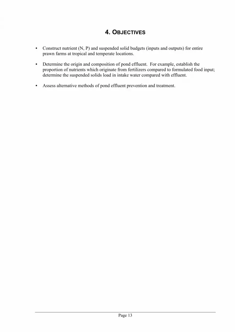
4. OBJECTIVES
• Construct nutrient (N, P) and suspended solid budgets (inputs and outputs) for entire prawn farms at tropical and temperate locations.
• Determine the origin and composition of pond effluent. For example, establish the proportion of nutrients which originate from fertilizers compared to formulated food input; determine the suspended solids load in intake water compared with effluent.
• Assess alternative methods of pond effluent prevention and treatment.

Page 14
5. METHODS
5.1 Study locations and objectives During the project, studies were conducted at four different prawn farms. The work completed at each farm is summarised below. Sampling strategies and analyses performed are described later (see Detailed Methods, page 19).
5.1.1 TruBlu Prawn Farm
Figure 1. Sampling locations, TruBlu Prawn Farm, 1995/96 TruBlu Prawn Farm (TBPF), on the Clarence River, NSW, was studied during the 1995/96 production season. The farm is located approximately 8 km from the river mouth. Production at TBPF was seasonal. Ponds were typically filled and stocked during spring (October to December) and harvested in autumn (April to June), and were allowed to dry out during the winter months. Only Penaeus monodon were produced until the 1995/96 season when P. japonicus were also stocked. During the period of study, 3.9 ha were stocked with P. monodon and 18.2 ha were stocked with P. japonicus, at an average stocking density of 35.4 prawns m-2. The objectives of the sampling were to: • Determine whole-farm nutrient and suspended solid budget: weekly water samples were taken
from the main intake and main discharge sampling points (Figure 1). These samples were analysed for TN, TP and TSS1.
• Effluent composition and daily variation of farm intake and discharge: intake and discharge streams were monitored intensively during two week-long periods, in February and April 1996. Two samples were taken each day from the main intake and main discharge
1Appendix A2 explains abbreviations
Main intake
Main discharge
Secondary discharge
Secondary intake

Page 15
sampling points, and an additional daily sample was taken from both the secondary intake and secondary discharge sampling points (Figure 1). These samples were analysed for TN, TP, total suspended solids (TSS), and total particulate organics (TPO). A subset of samples was also analysed for chlorophyll a and bacteria.
5.1.2 Seafarm
Figure 2. Aqualab installation and sampling locations, Seafarm, 1996/97. Seafarm (Hinchinbrook Channel, Cardwell, QLD) was studied during the 1996/97 production season. At the time of our study the production cycle was unsynchronised (ie, different ponds had different-aged prawns) and production was year-round. Penaeus monodon were grown in 48 ponds (total area, 56.4 ha). Average water depth was 1.4 m, and normal stocking density was 32 � 35 m-2. Pond water quality, and prawn growth parameters, were described by Jackson & Wang (1998). The objectives of the sampling were to: • Determine a whole-farm, whole-season nutrient and suspended solid budget: weekly
water samples were taken from the Intake stage 1 and Discharge sampling locations (Figure 2). These samples were analysed for TN, TP and TSS
• Determine the composition of farm intake and discharge: intake and discharge streams were monitored intensively during two week-long periods, in February and August 1997. Three samples were taken each day from the Discharge sampling point; two samples each day from Intake stage 2; and 1 sample each day from Intake stage 1. In addition, during the sampling week in August, the Fresh water intake (fresh creek water discharging into the intake canal) was sampled on four days (Figure 2). These samples were analysed for TN, TP, TSS, dissolved N (DN), dissolved P (DP), TAN, chlorophyll a, bacteria, total organic carbon (TOC), nitrate (NO3
-), nitrite (NO2-) and TPO content.
• Quantify short-term temporal variability of intake and discharge water quality: the Aqualab was installed midway between the intake and discharge canals (Figures 2,3). Pumps and sample pipelines (blue lines,) were used to bring water-quality samples from the farm intake and discharge to the Aqualab for analysis. The Aqualab was programmed to sample every three hours. This was our first experience using the Aqualab, and we discovered consistent operation at such a remote locality was difficult to achieve because the machine required frequent maintenance. Nevertheless, valuable data were obtained. The Aqualab monitoring is described in detail below, under Aqualab sampling (page 21).
Intake sampling (stage 1)
Discharge sampling location
Aqualab sample pipelines
Aqualab
Intake sampling (stage 2)
Fresh waterintake

Page 16
Figure 3. Aqualab
installation, Seafarm
5.1.3 Rocky Point Prawn Farm Rocky Point Prawn Farm (RPPF), on the Logan River, QLD, was studied during the 1997/98 production season. The farm primarily grows P. japonicus, with 10 to 20% of production area devoted to P. monodon. Production is seasonal, with the filling, stocking and harvesting occurring at times similar to TBPF (above). The farm receives water through a narrow canal, 1.2 km long, passing through sugar cane farmland. A partial recirculation strategy was employed: after discharge from production ponds, water was passed through one of several treatment ponds before being returned to the supply storage. Recirculation was used primarily when good source water quality was unavailable, due to rainfall or runoff from agricultural land into the supply canal. When intake water quality was adequate, normal water exchange was practiced. The objectives of the sampling were to: • Determine whole-farm nutrient and suspended solid budget: weekly water samples were
taken from the intake and discharge sampling points (Figure 4). These samples were analysed for TN, TP and TSS.
• Examine the performance of treatment ponds: Four treatment ponds had been constructed at RPPF (A, B, C and D: Figure 4). Changes in water quality were studied as water passed through these treatment ponds. The main sampling was conducted during two week-long periods, in January and March 1998. Treatment ponds A, B and C were sampled at the inlet and outlet, once per day, and analysed for TN, TP, TSS, TPO and TAN.
Figure 4. Rocky Point Prawn Farm: treatment ponds (A, B, C, D) and Budget sampling locations. (Treatment pond A and adjacent production pond were constructed after this aerial photograph was taken).
A
B
C
D
Intake sampling location
Discharge sampling location (400 m downstream)

Page 17
Treatment pond D, total area 0.49 ha, was selected for detailed sampling. This treatment pond serviced five production ponds with a total area of 3.4 ha (Figure 5). Figure 5. Treatment pond D, showing
water flow from 5 production ponds. Treatment pond D had two sections separated by a weir (Figure 6). The first section, the Settlement pond, was about 1.5 m deep. It was intended to promote settlement of particulate matter and growth of filter-feeding organisms. The second section, the Aquatic-plants pond, was 0.3 m deep and was intended to promote removal of nutrients by growth of aquatic plants
Settlement pond (0.372 ha) Aquatic-plants pond (0.118 ha)
Figure 6. Treatment Pond D, Rocky Point Prawn Farm. Arrows indicate water flow; numbers indicate sampling locations (see text).
Samples were taken from three locations in this pond: at the input of the settlement pond; at the discharge of the settlement pond; and at the discharge of the aquatic-plants pond (1, 2, 3 respectively: Figure 6). Samples were taken twice per day during two one-week periods in January and March 1998. Sediment samples (cores and traps) were also taken. Details of this sampling are provided below, under Treatment pond sampling. In addition, the Aqualab was installed at this pond for most of the production season, sampling the same three locations (1, 2, 3: Figure 6).
5.1.4 Gold Coast Marine Prawn Farm Gold Coast Marine Prawn Farm (GCMPF) on the Logan River, Queensland, was also studied during 1997/98. The objective of the sampling was to assess the performance of a settlement pond (newly-constructed, under the guidance of the project team: Figure 7). The main part of this pond was a settlement basin, without additional structure (0.809 ha); however, panels of mesh and shadecloth were installed in the discharge zone (0.226 ha) (Figures 7, 8).
D
3
2 1

Page 18
Figure 7. Treatment pond, Gold Coast Marine Prawn Farm, sampled during 1997/98. Water flow rate through the system was 250 L s-1. Triplicate water-quality samples were taken every month from the intake, middle and discharge locations, and analysed for TSS, TPO, chlorophyll a (chla), TN, TP, DN, DP, TAN, oxides of nitrogen (NOx), and FRP. In addition, sediment samples were taken (from cores and traps).
Figure 8. Structures built in discharge zone of GCMPF treatment pond.
Intake sampling location
50 m
Middle sampling location
Discharge sampling location
Structure zone

Page 19
An additional study (not part of the original research plan) was conducted at GCMPF during the 1998/99 production season. The objective of this sampling was to assess the performance of a pilot-scale fully-lined settlement pond, approx. 0.103 ha and 2 m deep (Figure 9). It was built to trial the strategy of periodic draining and manual removal of sediment (intended to reduce the remineralisation of nutrients). The flow rate of pond discharge water through the pilot facility was 1.04 ML per day.
Figure 9. Gold Coast Marine Prawn Farm pilot sedimentation pond, drained
after 6 weeks of operation (objects scattered on pond floor are sandbags to weight the pond lining before filling).
5.2 Detailed methods
5.2.1 Whole-farm budget sampling
5.2.1.1 Water flow Water flow through the farms was monitored continuously using Doppler flow dataloggers (Starflow 6526A, Unidata Pty Ltd). At TBPF, a logger was installed in each of two concrete discharge pipes (Main discharge and Secondary discharge, Figure 1); at Seafarm, one logger was installed in the bed of the main discharge canal (Discharge sample location, Figure 2); and at RPPF, a logger was installed in a concrete pipe providing the farm intake (Intake sample location, Figure 4). Water velocity and depth were recorded every 5 min, allowing daily flows to be calculated (see Appendix A3 for details of calculations). In addition, at each farm the activity of water supply pumps was monitored: a datalogger recorded the date and time on each occasion that any supply pump was turned on or off. Pump activity times were used with manufacturers' calibrations to calculate daily farm intake. At Seafarm and TBPF, these data provided an independent check of farm water use. However, at RPPF, the pump data could not be used in this way since water discharged from pumps was both discharged from the farm and recirculated within the farm, in unpredictable and varying proportions.

Page 20
5.2.1.2 Water samples Triplicate samples of farm intake and discharge water were taken each week. At Seafarm and TBPF the samples were taken by farm staff and frozen on-site, then transferred to the Cleveland laboratory at regular intervals. The samples from RPPF were taken by project staff, placed on ice immediately, and transported to the laboratory where they were frozen. All samples were analysed for TSS, TP and TN by the methods described below. 5.2.1.3 Sediment samples Samples of sediment were collected from the central zone (where flocculated sludge accumulated) of 6 ponds at Seafarm and TBPF, after the ponds had been drained. The samples were collected from more than 5 sites within a pond, then combined. The resulting composite sample was analysed for TN, TP, and percent organic matter by the methods described below. 5.2.1.4 Farm management data Farm managers provided data for food, fertilizer usage, sediment removal, and prawn harvest. Commercially sensitive information, particularly feed inputs and harvest quantities, are not detailed in this report � although they were made available to the peer-review panel for assessment.
5.2.2 Intensive sampling At each farm, intensive sampling was conducted during two separate week-long intervals: at TBPF, from 1/2/96 to 7/2/96 and from 31/3/96 to 6/4/96; and at Seafarm, from 13/2/97 to 26/2/97 and from 29/7/97 to 4/8/97. During these periods, triplicate samples of farm intake and discharge water were taken three times each day. Normally the first sample of the day was taken before 8 am, and the other two were spread through the day � although samples were only taken when water was flowing through the canals. Samples were filtered on-site within 1 h of collection, and the resulting filtrates and residues were frozen and transported to the Cleveland laboratory for analysis. The TBPF samples were analysed for TN, TP and TSS; and a subset of samples was analysed for TOC, DOC, Chla, TPO and bacteria. The Seafarm samples were analysed for TN, TP, DN, DP, TSS, TPO, TAN, and Chla; a subset of samples was also analysed for bacteria, TOC, NOx and NO2. Analysis methods are detailed below.
5.2.3 Treatment pond sampling
5.2.3.1 Rocky Point Prawn Farm Water sampling of treatment ponds at RPPF was conducted during two separate week-long intervals: 24/1/98 to 4/2/98 and 21/3/98 to 27/3/98. During these periods: • Triplicate samples of water were taken three times each day, from three locations within
treatment pond D (1, 2, 3, Figure 6). Morning samples were taken near-dawn; the remaining samples were evenly spread through the day. These samples were analysed for TN, TP, DN, DP, TSS, TPO, TAN, and Chla. A subset of samples was also analysed for TOC, DOC, NOx, NO2, and urea.
• Once per day, triplicate samples were also taken from the inlet and discharge of the other three treatment ponds (A, B, C, Figure 4). These samples were analysed for TN, TP, TSS, TPO and TAN.
All samples were filtered on-site within 1 h of collection, and the resulting filtrates and residues were frozen and transported to the Cleveland laboratory. The analysis techniques are described below.

Page 21
Sediment cores (sampled to depth of sludge (3-4 cm), 30 mm, 5 cores combined) were collected from the start, middle and end of treatment pond D at RPPF before the pond was first filled, and after it had been drained at the end of the production season. Sediment traps (8 L galvanised buckets, 20 cm mouth diameter, resting on pond substrate) were deployed at the beginning, middle and end of treatment pond D on 4 occasions throughout the season. The sediment core samples and trap samples were analysed for TN, TP and percent organic matter. Plant material was harvested from the shallow section of the treatment pond on three occasions and on one occasion from the deep section. The plants were harvested on the first two occasions by hand, using a net. The 3rd and 4th harvest was carried out with an excavator. The plant material was allowed to partially dry for several days on the banks of the treatment pond, and was then collected and weighed. The plant material was sub-sampled and analysed for moisture content, TN, TP and TOC by methods described below. 5.2.3.2 Large settlement pond, Gold Coast Marine Prawn Farm, 1997/98 The flow rate of pond discharge water through the settlement pond was 250 L.s-1, or 21.6 ML.d-1. Triplicate water samples were taken each month from the Intake, Middle and Discharge sampling locations (see Figure 7), and analysed for TSS, TPO, Chla, TN, DN, TAN and NOx. Sediment cores were taken from the same locations, at the start and end of the season; and sediment traps were deployed at the same locations during February, March and May 98. Sediment samples were analysed for TN, TP, TPO and TOC. 5.2.3.3 Pilot settlement pond, Gold Coast Marine Prawn Farm, 1998/99 Triplicate water-quality samples were taken every week from the intake and discharge locations, from 7 Jan 99 to 6 Apr 99. The samples were analysed for both particulate and dissolved nutrient species with emphasis placed on nitrogen: TSS, TPO, Chla, TN, TP, DN, DP, TAN, NOx, and filterable reactive phosphate (FRP). The suspended solids were measured and divided into inorganic and organic components. During the drainage periods, the sediment depth was measured and sediment samples were collected for TN, TP, % Organic-content, moisture and density. After 6 weeks, the pond was drained and sediment removed; the pond was then refilled and normal operation continued. The flow rate of pond discharge water through the pilot facility was 1.04 ML per day.
5.2.4 Aqualab sampling An Aqualab� 2 was used to record 3-hourly data for a range of water-quality parameters. The Aqualab draws sample water through a series of analysis modules and between analysis cycles, all wetted parts are bathed in antibacterial solution to prevent fouling of sensors. The parameters measured, method used, and calibration methods are indicated in Table 1. Most parameters are validated or calibrated every measurement cycle. Due to continual development and enhancement of the instrument�s capabilities, different suites of parameters were measured at different times. The Aqualab was unavailable for the first study site, TBPF.
2 Greenspan Technology Pty Ltd, 22 Palmerin St, Warwick, QLD

Page 22
Table 1. Aqualab parameters, measurement method, and validation. Only a subset of parameters were used in this study � see text for details. Parameter Method used Calbration or validation Ammonia Ion-sensitive electrode (NH3) 2-point calibration using 1.7 and
2.4 ppm standard, before each measurement
Phosphate Spectrophotometric 2-point calibration using 0.06 and 0.12 ppm standard, before each cycle
Turbidity Nephelometric cell Filtered wash solution assessed before each cycle
PH pH electrode pH 4 standard assessed before each cycle
Dissolved oxygen
DO electrode Aerated water assessed before each cycle
Redox Redox electrode Salinity Inductive cell Temperature Pt cell At each Aqualab installation, high-pressure pumps (Grundfos CHI 2-50) were installed on the bank adjacent to the remote sampling points, and were used to pump sample water to the Aqualab. The pumps operated continuously. At the Aqualab location, the pumped water was delivered into continuously-overflowing containers, from which the Aqualab drew samples for analysis. The pipe system used to carry the sample from the pump to the Aqualab changed during the study; details for each study site are provided below. 5.2.4.1 Seafarm The sample pumps were installed at the farm intake and discharge canals, and the Aqualab was installed midway between the two sampling locations (Figure 2). At each sampling point, the pump intake was connected by a short length of 25 mm polyethylene pipe to a coarse intake screen, constructed from a 0.6 m length of 40 mm PVC pipe, liberally drilled with 10 mm holes. The intake screens were securely located, 0.3 m from the bottom, by attachment to steel star-pickets. During initial trials, the Discharge intake screen occasionally became blocked by filamentous algae. This was overcome by installation of a coarse mesh �fence� surrounding the intake point (Figure 10).
Figure 10: Discharge intake with mesh fence surrounding intake point at Seafarm
Sample water was pumped to the Aqualab through 25 mm polyethylene pipes. The pump capacity and pipe diameter were chosen to produce > 3 m.s-1 water velocity in the pipe, reportedly sufficient to avoid the growth of fouling organisms (Huguenin & Colt, 1989). The following parameters were measured: phosphate, turbidity, pH, and dissolved oxygen (the

Page 23
procedure for measuring ammonia was still under development and was unavailable at this time). The Aqualab was installed on 23/10/96 but due to installation problems, data collection did not commence until February. The device was removed on 6/8/97. The strategy of relying on high flow rate to stop biofouling within the sample delivery pipes was successful for several weeks, however eventually fouling organisms became established. Once this process had begun, the reduced flow velocity allowed further biofouling to develop rapidly. Fouling organisms within the sample delivery pipes intermittently affected all the parameters being monitored, and regular cleaning was required. Therefore accurate data was only produced for 3 months. 5.2.4.2 Rocky Point Prawn Farm, Treatment pond D The Aqualab was installed near the weir between the two pond sections (Figures 5,6). Sample pumps were located at the three sampling points (1 ,2 ,3 , Figure 6). In this deployment, due to the failure of the previous strategy for preventing biofouling in the sample-delivery pipes, a new system was used, based on duplication of the pipes on both intake and discharge sides of the pump (Figure 11).
Figure 11. Dual-pipeline system for Aqualab sample collection, RPPF, 1997/98. Off-duty pipelines shaded grey; see text for description of operation.
At any particular time, water flowed through only one intake pipeline and one discharge pipeline, while the alternate pipelines were off duty (shaded grey, Figure 11). The anoxic, stagnant water within the off-duty pipe killed any newly-settled fouling organisms. Every 7 d, the 2-way selector valves were both switched to the opposite positions, thereby alternating the functions of the pipelines. The new on-duty pipeline was flushed for at least 1 h before Aqualab water samples were taken. This system completely overcame any problems with biofouling; even after 6 months, the pipes were completely clean.
2-WAY SELECTOR VALVES
AQUALAB SAMPLE
OVERFLOW TO WASTE
PUMP
INTAKE SCREENS

Page 24
5.2.5 Analysis methods
5.2.5.1 Phosphorus and Nitrogen (water samples) Two methods were used for total phosphorus analysis. Samples from the first intensive field trip to TBPF were sent to a NATA-accredited commercial laboratory where they were analysed by standard methods. Subsequent samples were processed at the CSIRO laboratory using a persulphate digestion method (APHA, 1995) and analysed by standard method 4500-P E (APHA, 1989). 15 ml of sample and 5 ml of digestion reagent were used for a 50 min digestion period at 120 ºC. Similarly, two methods were used for total nitrogen analysis. Samples from the first intensive field trip to TBPF were sent to a NATA-accredited consulting laboratory and were analysed by standard Kjeldahl methods. Subsequent samples were processed at the CSIRO laboratory using the persulphate digestion method described for total phosphorus, with subsequent analysis of N digestion product (nitrate) using method 4500-NO3
-E (APHA, 1995). The efficiency of the cadmium column was assessed by comparing a 2 mg.L-1 NO3 standard against a 2 mg.L-1 NO2 standard at the commencement of each set of analysis. Dissolved phosphorus and nitrogen were analysed using the persulphate-digestion methods described above, after filtering through glass fibre filters (GF/F). 5.2.5.2 TSS and Particulate Organic matter Total suspended solids were determined by standard method 2540-E (APHA, 1995).Filter residues were ignited at 550 ºC to determine volatile solids as an estimate of particulate organic matter. 5.2.5.3 TAN, NOx Total ammoniacal nitrogen(TAN) was determined using indophenol blue analysis, method 1.4 (Parsons, Maita & Lalli, 1984). Total oxides of nitrogen were determined by the standard cadmium reduction method 4500-NO3-E (APHA, 1995). 5.2.5.4 Reactive Phosphate Reactive PO4-P analysis were performed by standard method 4500 � P E. (APHA, 1989). 5.2.5.5 Chlorophyll Chlorophyll a was assessed by extraction of filters in cold acetone and spectrophotometric analysis at 630, 647,664 and 750 nm, method 10200 H.2 (APHA, 1989). Initial tissue maceration was achieved using a Branson Sonifier cell disrupter B15 in pulse mode. 5.2.5.6 Bacteria Bacteria were stained with 50-100µL of 0.1 mg.mL-1 acridine orange solution for 1 min (Hobbie, Daley & Jasper 1977) and counted under an epifluorescence microscope with a 50X oil-immersion objective lens. 5.2.5.7 Sediments Sediment TN and TP analyses were performed by a NATA-accredited consulting laboratory using freeze drying for sediment preparation and standard Kjeldahl analysis. Freeze drying helped conserve the high levels of TAN in the sediment. The percentage organic content of the pre-dried sediments were determined by loss on ignition at 550 ºC as per method 2540 G. (APHA, 1995). 5.2.5.8 Plant material Analysis of TN, TP and TOC in plant material was performed by a NATA-accredited laboratory using the same methods as described above. The moisture content was determined

Page 25
by weighing 3 replicate samples of plant material onto pre-weighed aluminium trays and then drying at 40oC to constant weight.
5.2.6 Analysis verification As described above, two different methods were used during the study for analysis of total Nitrogen and total Phosphorus. To confirm the comparability of these two methods, a subset of samples from the first intensive field trip to TBPF, (originally analysed by total kjeldahl Nitrogen and Phosphorus techniques) were also analysed by the persulphate TN and TP method. The results always agreed within 10%. Quality control samples (QC samples: natural brackish water, filtered, unfiltered, with known TN, TP, DN, DP, TAN, nitrogen oxides and reactive PO4 content) were purchased from the Queensland Health and Scientific Services Laboratory and were used to validate all nutrient analyses. Results were always accurate within 10%.
In a further confirmation of the accuracy of analyses, our laboratory participated in the 1999 National Low-Level Nutrient Collaborative Trials, organised in collaboration with Standards Australia. For Total Nitrogen, our results were all classified optimal except one (the lowest concentration) which was classified satisfactory; all were within 6% of the correct result. Two of our four Total Phosphorus results (those based on prawn farm water) were also classified optimal; the remainder (those spiked with a particularly refractory P compound, unlikely to be present in prawn farm pond or discharge water) were within 25% of the correct result.

Page 26
6. RESULTS AND DISCUSSION
6.1 Nutrient and TSS budgets
6.1.1 TruBlu Prawn Farm, 1995/96 season
6.1.1.1 Flooding during May 1996 Our study at TruBlu Prawn Farm coincided with extremely high local rainfall during May 1996, which resulted in the highest flood of the Clarence River since 1976 (7.07 m), Figure 1:
Figure 1. A, daily rainfall (mm) at Yamba during 1996; B, Flood history, Clarence River
The rainfall caused severe local flooding at the farm, and salinity in the adjacent river was zero for most of May 1996. As a result, negligible water was pumped from the river, and discharge from the farm was dominated by flood drainage for many weeks. The farm suffered major production losses from crop mortality. Because the latter part of the production season suffered such unusual conditions, only data collected before the heavy rain began on 1 May 1996 are presented in this report. For the same reason, it was not meaningful to calculate a whole-farm nutrient budget for the whole season. 6.1.1.2 Import and export due to water exchange
6.1.1.2.1 Water budget The records from the pump activity dataloggers were used to calculate the water volume pumped into the farm. Pump 3 (the largest pump, located at the Main intake; see Figure 1, Methods) provided the largest volume. Pumps 1 and 2, smaller pumps at the same location,
1/1/1996
1/2/1996
1/3/1996
1/4/1996
1/5/1996
1/6/1996
1/7/1996
0
50
100
Yamba daily rainfall(mm)
Jul 96 Jan 96 Feb 96 May 96Mar 96 Apr 96 Jun 96
Mar 74
Feb 76
Jun 7
6
May 80
Jun 8
3Apr
88Apr
89
May 96
0
5
Floo
d he
ight
at G
rafto
n (m
) Flood history, Clarence River

Page 27
also provided significant water volumes. Pump 4, located at the Secondary intake (Figure 1, Methods) supplied only minor water volume (Figure 2).
Figure 2. Intake water volumes and sources, TruBlu Prawn Farm, 1996. Note: Pump 4 logging only commenced 19 March 1996.
Total farm intake compares closely with farm discharge (Figure 3). Since intake and discharge were measured by different methods, our confidence in the accuracy of these data is high.
Figure 3. Intake and discharge water volume, TruBlu Prawn Farm, 1996. Note: Intake logging commenced 25 Jan 1996; Discharge logging commenced 3 Feb 1996
6.1.1.2.2 Intake and discharge nutrient concentrations Intake TSS was very high during January and February 1996 (around 100 mg.L-1: Figure 4); during this time, rainfall in the Clarence River catchment was high and the river was very turbid. After the end of February, intake TSS dropped to about 50 mg.L-1. TSS levels in discharge water were fairly consistent at about 100 to 130 mg.L-1 throughout the study. Total phosphorus levels in intake water were also relatively high during the early period. Discharge levels of total nitrogen decreased slightly during the study (Figure 4).
0
10
20
30
40
50
60
70Pump 1
Pump 2
Pump 3
Pump 4
AprMar MayFeb
01020304050607080
Jan Feb Mar Apr May
Intake
Discharge

Page 28
19/1
/96
2/2/
963/
2/96
4/2/
965/
2/96
6/2/
967/
2/96
23/2
/96
1/3/
968/
3/96
15/3
/96
22/3
/96
31/3
/96
1/4/
962/
4/96
3/4/
964/
4/96
5/4/
966/
4/96
19/4
/96
26/4
/96
28/5
/96
31/5
/96
0
100
200 IntakeDischarge
TSS (mg/L)
19/1
/96
2/2/
963/
2/96
4/2/
965/
2/96
6/2/
967/
2/96
23/2
/96
1/3/
968/
3/96
15/3
/96
22/3
/96
31/3
/96
1/4/
962/
4/96
3/4/
964/
4/96
5/4/
966/
4/96
19/4
/96
26/4
/96
28/5
/96
31/5
/96
0
2
4 TN (mg/L)
19/1
/96
2/2/
963/
2/96
4/2/
965/
2/96
6/2/
967/
2/96
23/2
/96
1/3/
968/
3/96
15/3
/96
22/3
/96
31/3
/96
1/4/
962/
4/96
3/4/
964/
4/96
5/4/
966/
4/96
19/4
/96
26/4
/96
28/5
/96
31/5
/96
0.0
0.2
TP (mg/L)
1/2/1996 1/3/1996 1/4/19960
5000
10000
15000 IntakeDischargeTSS (kg/d)
1/2/1996 1/3/1996 1/4/19960
5
10
15 TP (kg/d)
1/2/1996 1/3/1996 1/4/19960
50
100TN (kg/d)
Figure 4. Intake and
discharge nutrient concentrations (with standard errors), TruBlu Prawn Farm, 1996. Data are for Main intake and Main discharge locations (see Figure 1, Methods).
6.1.1.2.3 Nutrient import and export The daily water-borne budgets of TSS and nutrients, over the whole growout season, were derived by first calculating the total volume of intake and discharge water (see Figure 3) for each 24 h period. Each daily volume was then multiplied by the most recent data for nutrient concentration (see Figure 4). The results for main and secondary intakes, and for main and secondary discharges (Figure 1, Methods), were summed respectively (Figure 5). Figure 5. Nutrient
budgets for TruBlu Prawn Farm, 1996
For most of February, there was actually more TSS imported to the farm than exported; the average daily intake of TSS was 2,670 kg.d-1, while the average daily discharge was only 1,800 kg.d-1 (Figure 5). During March, however, the net export became positive: average daily intake reduced to 1,450 kg.d-1, and daily export increased to 2,740 kg.d-1. Export of TSS increased markedly during April, due to a combination of higher discharge volumes (Figure 3)

Page 29
0
2000
4000
6000
8000
TSS (kg/d)Y o u r te x t
0
5
10
TP (kg/d)Y o u r te x t
February March April0
102030405060
TN (kg/d)Y o u r te x t
and higher concentrations of TSS in discharge water (Figure 4); although imported TSS did not change much (1,500 kg.d-1), the exported TSS increased to 6,720 kg.d-1 (Figure 5). The temporal pattern of intake and discharge of total P is similar to that of TSS (Figure 5). During February, the daily import and export were 1.91 and 4.15 kg.d-1 respectively; during March, the intake reduced to 0.93 kg.d-1 while export increased to 4.78 kg d-1. During April, while the intake of P remained similar (0.92 kg.d-1), the daily discharge almost doubled to 9.0 kg.d-1. In contrast, the farm�s intake and discharge of total N followed a different pattern (Figure 5). Daily intake did not vary much through the season: 10.23 kg.d-1 in February 1996, 7.06.kg d-1
in March, and 8.17 kg.d-1 in April. However the average daily discharge of N increased: 41.47 kg.d-1 in February, 50.74 kg.d-1 in March, and 62.39 kg.d-1 in April. The net monthly discharges of each of the three components were calculated by subtracting the intake average from the monthly discharge average (Figure 6). Figure 6. Net nutrient
exports, TruBlu Prawn Farm, 1996
The net discharge of each parameter rose steadily during the season: TSS from �870 kg.d-1 to over 5000 kg.d-1; total P from 2.24 to 8.07 kg.d-1; and total N from 31.24 to 54.22 kg.d-1.
Page 30
6.1.2 Seafarm, 1996/97 season
6.1.2.1 Import and export due to water exchange
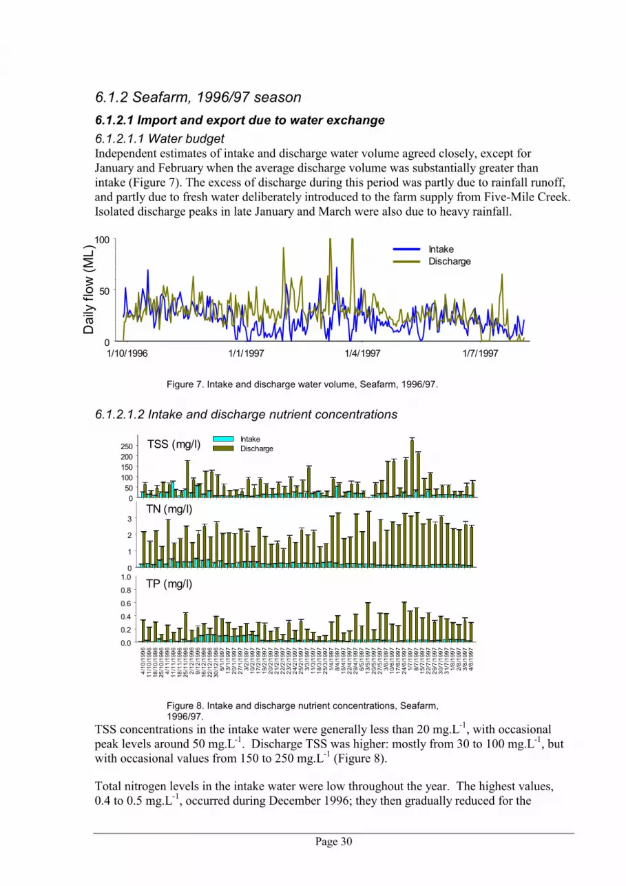
6.1.2.1.1 Water budget Independent estimates of intake and discharge water volume agreed closely, except for January and February when the average discharge volume was substantially greater than intake (Figure 7). The excess of discharge during this period was partly due to rainfall runoff, and partly due to fresh water deliberately introduced to the farm supply from Five-Mile Creek. Isolated discharge peaks in late January and March were also due to heavy rainfall.
Figure 7. Intake and discharge water volume, Seafarm, 1996/97. 6.1.2.1.2 Intake and discharge nutrient concentrations
Figure 8. Intake and discharge nutrient concentrations, Seafarm, 1996/97.
TSS concentrations in the intake water were generally less than 20 mg.L-1, with occasional peak levels around 50 mg.L-1. Discharge TSS was higher: mostly from 30 to 100 mg.L-1, but with occasional values from 150 to 250 mg.L-1 (Figure 8). Total nitrogen levels in the intake water were low throughout the year. The highest values, 0.4 to 0.5 mg.L-1, occurred during December 1996; they then gradually reduced for the
050
100150200250
IntakeDischargeTSS (mg/l)
0
1
2
3TN (mg/l)
4/10
/199
611
/10/
1996
18/1
0/19
9625
/10/
1996
4/11
/199
611
/11/
1996
18/1
1/19
9625
/11/
1996
2/12
/199
69/
12/1
996
16/1
2/19
9622
/12/
1996
30/1
2/19
966/
1/19
9713
/1/1
997
20/1
/199
727
/1/1
997
3/2/
1997
10/2
/199
717
/2/1
997
19/2
/199
720
/2/1
997
21/2
/199
722
/2/1
997
23/2
/199
724
/2/1
997
25/2
/199
73/
3/19
9711
/3/1
997
18/3
/199
725
/3/1
997
1/4/
1997
8/4/
1997
15/4
/199
722
/4/1
997
29/4
/199
76/
5/19
9713
/5/1
997
20/5
/199
727
/5/1
997
3/6/
1997
10/6
/199
717
/6/1
997
24/6
/199
71/
7/19
978/
7/19
9715
/7/1
997
22/7
/199
729
/7/1
997
30/7
/199
731
/7/1
997
1/8/
1997
2/8/
1997
3/8/
1997
4/8/
1997
0.0
0.2
0.4
0.6
0.8
1.0TP (mg/l)
1/10/1996 1/1/1997 1/4/1997 1/7/19970
50
100
Dai
ly fl
ow (M
L) IntakeDischarge

Page 31
remainder of the study period, to about 0.1 to 0.2 mg.L-1 by August 1997. In contrast, the discharge nitrogen concentration gradually increased during the study period, reaching the highest sustained values (2.5 to 3 mg.L-1) during July (Figure 8). Intake concentration of total phosphorus was mostly below 0.03 mg.l-1 except during summer (December 1996 to February 1997) when it was consistently about 0.1mg.l-1. Discharge concentration of total phosphorus followed a similar pattern to that of TN, peaking (slightly above 0.4 mg.l-1) during July 1997 (Figure 8). 6.1.2.1.3 Nutrient import and export Figure 9. Nutrient
budgets, Seafarm, 1996/97.
As was done for the TruBlu data, the total daily volume of intake and discharge water (see Figure 7) was combined with the most recent data for nutrient concentration (see Figure 8) to calculate the daily water-borne budgets of TSS and nutrients (Figure 9). The contribution of intake loads to the amount finally discharged was greatest for TSS, where the average intake amount was 34.7% of the discharge. In contrast, only 11.5% of discharged nitrogen originated in intake water. Intake contribution to phosphorus discharge was also low: 12.5%. The net water-borne budget for TSS and nutrients was calculated by subtracting intake quantities from discharge quantities, and averaging the result for each month of the study. Net discharge of TSS generally varied from about 1,000 to 2,000 kg.d-1, with a maximum discharge of about 3,000 kg.d-1 during June. Net discharge of nitrogen generally varied between about 50 and 70 kg.d-1, while net phosphorus discharge was normally between about 5 and 8 kg.d-1 (Figure 10).
02000400060008000
IntakeDischarge
TSS (kg/d)
1/10/1996 1/1/1997 1/4/1997 1/7/19970
5
10
15TP (kg/d)
0
50
100
150TN (kg/d)

Page 32
Figure 10. Net
daily exports, Seafarm, 1996/97.
6.1.2.2 Food additions Total food added to all ponds was recorded over the entire study period: from 1 Oct 96 to 31 Jul 97. Nutrient addition via food was calculated assuming 6.9% N and 1.5% P (as proportion of pellet wt, including 9% water: unpublished data, D. Smith and M. Barclay, CSIRO). 6.1.2.3 Sediment removal At the time of our study, there were extensive prawn health problems (mid-crop mortality syndrome) at farms throughout Queensland. One strategy adopted by Seafarm to deal with this epidemic was to remove all traces of accumulated sediment after each harvest. Therefore, extraordinarily large volumes of sediment were being removed from Seafarm�s ponds during our study: about 50m3 of moist sediment per crop per pond (60t dry wt). This resulted in substantial net removal, and does not represent the �normal� removal of a single crop�s accumulated sediment. In fact recently, farm management have found it necessary to return substantial amounts of sand and gravel to ponds, to restore their original dimensions. Studies on sediment accumulation rates at other P. monodon farms suggest that sediment deposition rates were generally between 35 and 60 t (dry wt) each crop. (unpublished data, M. Burford, CSIRO). Therefore, in calculating the whole-farm nutrient budgets, we have assumed that 45 t were removed each time a pond was harvested. In addition, we have examined the sensitivity of the budget model to a range of assumptions from 35 to 60 t. Net nutrient export in the sediment (calculated from analyses of sediment and native soil) was 1,327 mg.kg-1 N, and 1,232 mg.kg-1 P. 6.1.2.4 Prawn harvest Total prawn harvest quantities, from all ponds, were recorded over the entire study period: from 1 Oct 96 to 31 Jul 97. The nutrient content of harvested prawns was calculated assuming 2.9% N and 0.34% P (as a proportion of wet wt, including 74% water: unpublished data, D. Smith and M. Barclay, CSIRO).
0100020003000 TSS (kg/d)
Oct 96
Nov 96
Dec 96
Jan 97
Feb 97
Mar 97
Apr 97
May 97
Jun 97
Jul 97
02468 TP (kg/d)0
20406080 TN (kg/d)

Page 33
6.1.2.5 Overall budget summary, Seafarm, 1996/97 season
6.1.2.5.1 Nitrogen budget
Figure 11. Sources of input nitrogen, Seafarm. Existing stock represents the N contained in on-farm prawn biomass at the time the study began.
Figure 12. Nitrogen destinations, Seafarm. Percentages are related to total input N. Remaining stock represents the N contained in on-farm prawn biomass at the time the study finished. D,V is the estimated loss of N to denitrification and ammonia volatilisation.
90% of the Nitrogen entering the farm came from the formulated food (Figure 11); only 5% originated from intake water. At the time the study began, the existing prawn biomass also contributed 5% to the total N inputs over the study period. Only 22% of the input nitrogen was converted to prawns (Figure 12). By far the largest proportion (57%) was contained in discharge water over the whole season. Fourteen percent remained in the sediment, and 4% remained in unharvested prawns. Only 3% of input nitrogen was unaccounted for, and assumed to be lost to the atmosphere via denitrification and volatilisation of ammonia.
Sediment14%
Harvest22%
Discharge water57%
Remaining stock4%
D, V3%
Food90%
Existing stock5%
Intake water5%

Page 34
6.1.3 Rocky Point Prawn Farm, 1997/98 season
6.1.3.1 Import and export due to water exchange
6.1.3.1.1 Water flow through farm
Figure 13. Diagram indicating water flow at Rocky Point Prawn
Farm. P, production pond; T, treatment pond; R, recycled water; D, discharged water. See text for explanation.
At RPPF, the water flowed by gravity through the intake canal into the supply storage canal (Figure 13). From the supply storage, it was pumped into production ponds using one of four pumps distributed within the farm, each supplying two to four ponds (only one pump and 2 ponds are shown in the figure); water from each pond then flowed into an adjacent treatment pond (T, Figure 13). On exit from the treatment pond, there were two possible flow paths: to be recycled back into the supply storage (R, Figure 13) or to be discharged from the farm (D, Figure 13). The flow rates through each of these alternative paths (and hence the degree of water recirculation) were controlled by monk boards. Therefore, at RPPF, the pump activity dataloggers were inappropriate for determining the volume of water passing through the farm, since pumped water was recycled or discharge in unpredictable proportions. Unlike the previous two study sites, at this location we only had a single estimate of the farm�s water use: the doppler flow logger installed in a pipe in the farm intake (Figure 13; and intake sampling location, Figure 4, Methods).
Intake flow datalogger

Page 35
6.1.3.1.2 Water budget Datalogger records show that the amount of water used by the farm was generally 5 ML.d-1 or less before February (mean value, 3.8 ML.d-1), and about 8 to 12 ML.d-1 until early June (mean value, 9.3 ML.d-1) (Figure 14). No data are available for the first three weeks of February due to equipment failure.
Figure 14. Water flow through Rocky Point Prawn Farm, 1997/98
season 6.1.3.1.3 Intake and discharge nutrient concentrations Figure 15. Intake
and discharge nutrient concentrations, RPPF, 1997/98 season.
TSS in the water supplied to the farm from Logan River through the cane drainage canals was usually from 20 to 40 mg.L-1. Discharged levels were generally not much higher (Figure 15). The total N concentration in supply water was initially quite high: between 1 and 3 mg.L-1 up to the end of January (Figure 15). During this period, there was runoff from cane fields into the canals during the summer wet season. Later, as rainfall decreased and the farm�s water use flushed the canals, the total N intake dropped. Isolated peaks of N input to RPPF late in May were probably also due to heavy rainfall. Concentration of total N discharged was more consistent, generally being from 2.5 to 3.0 mg.L-1. Higher N discharges (between 4 and 5 mg.L-1) occurred early in the season and late in May 1998.
27/09/97 16/11/97 05/01/98 24/02/98 15/04/98 04/06/98 24/07/98
Date
0
5
10
15
ML
per d
ay
020406080
IntakeDischargeTSS (mg/l)
012345 TN (mg/l)
23/1
2/19
97
30/1
2/19
97
6/1/
1998
13/1
/199
8
20/1
/199
8
27/1
/199
8
10/2
/199
8
17/2
/199
8
24/2
/199
8
3/3/
1998
10/3
/199
8
17/3
/199
8
31/3
/199
8
7/4/
1998
16/4
/199
8
22/4
/199
8
30/4
/199
8
5/5/
1998
12/5
/199
8
19/5
/199
8
26/5
/199
8
2/6/
1998
9/6/
1998
0.0
0.1
0.2
0.3
0.4
0.5 TP (mg/l)

Page 36
Intake total P was usually between 0.5 and 1.0 mg.L-1; discharged P was generally between 0.2 and 0.3 mg.L-1, although it was slightly lower early in the season. 6.1.3.1.4 Nutrient import and export Figure 16.
Nutrient budgets, RPPF, 1997/98.
As was done with the data from the previous study sites, the total daily water volumes (see Figure 14) were combined with the most recent data for nutrient concentrations (see Figure 15) to calculate the daily water-borne budgets of TSS and nutrients (Figure 16). The contribution of each intake load of TSS, TN and TP to the amount finally discharged, averaged over the whole season, was the greatest of all the farms studied: 76.4% of TSS originated in the intake water, 37.0% of nitrogen, and 30.4% of phosphorus. Figure 17. Net
daily exports, RPPF, 1997/98.
The net budget for TSS and nutrients was calculated by subtracting intake quantities from discharge quantities, and averaging the result for each month of the study (Figure 17). The net discharge of TSS was negative for the first three months � that is, more TSS was imported to the farm than was exported. For the remainder of the study period, net TSS export varied between about 50 and 200 kg.d-1. Net discharge of nitrogen was also lowest during the first
0200400600800
IntakeDischarge
TSS (kg/d)
1/1/1998 1/4/1998 1/7/199801234
TP (kg/d)0
10203040
TN (kg/d)
Nov 97
Dec 97
Jan 9
8Feb 9
8Mar
98Apr
98
May 98
Jun 9
8Jul 9
80
1
2
3 TP (kg/d)0
10
20
30TN (kg/d)
-500
50100150 TSS (kg/d)

Page 37
three months (about 5 kg.d-1), and was mostly from 10 to 10 kg.d-1 thereafter. Similarly, the lowest values for net phosphorus export (0.2 to 0.4 kg.d-1) were during the first three months while during the remainder of the study period, between 1 and 2 kg of phosphorus were exported each day.
6.1.4 Budget comparison between the three farms To allow direct comparison of seasonal patterns between the three farms, regardless of the size of the farm, intake and net discharge nutrient quantities were expressed in terms of kg per ha of farm production area per day. 6.1.4.1 Seasonal patterns of nutrient import and export
6.1.4.1.1 Total Suspended Solids Figure 18. Intake and
net discharge of TSS (kg.ha-1.d-1), at 3 study sites: TruBlu Prawn Farm (TBPF), Seafarm, and Rocky Point Prawn Farm (RPPF).
For total suspended solids (TSS; figure 18), imports at TruBlu were at the highest level in February (121 kg.ha-1.d-1); import levels later in the year were about half this amount. Net discharge of TSS increased regularly through the season: from -37 kg.ha-1.d-1 in February 1998 (a net import of TSS) to 236kg.ha-1.d-1 in April 1998. At Seafarm, imported TSS was highest early in the wet season, from October to December, when import levels were 10 to 19 kg.ha-1.d-1. Later in the season, imports of TSS did not change much, generally being between 1 and 7 kg.ha-1.d-1. Net discharge of TSS did not show a distinct seasonal trend. At Rocky Point Prawn Farm, imports of TSS peaked in the middle of the production season (February to May) when levels were 20 to 25 kg.ha-1.d-1. Net discharge was negative for the
Feb 96 Mar 96 Apr 96-50
0
50
100TSSINPHAPD
TSSNETPHAPD
Intake
Net discharge
-50
0
50
100
TBPF, 1995/96
Seafarm, 1996/97
-50
0
50
100
RPPF, 1997/98
121 236
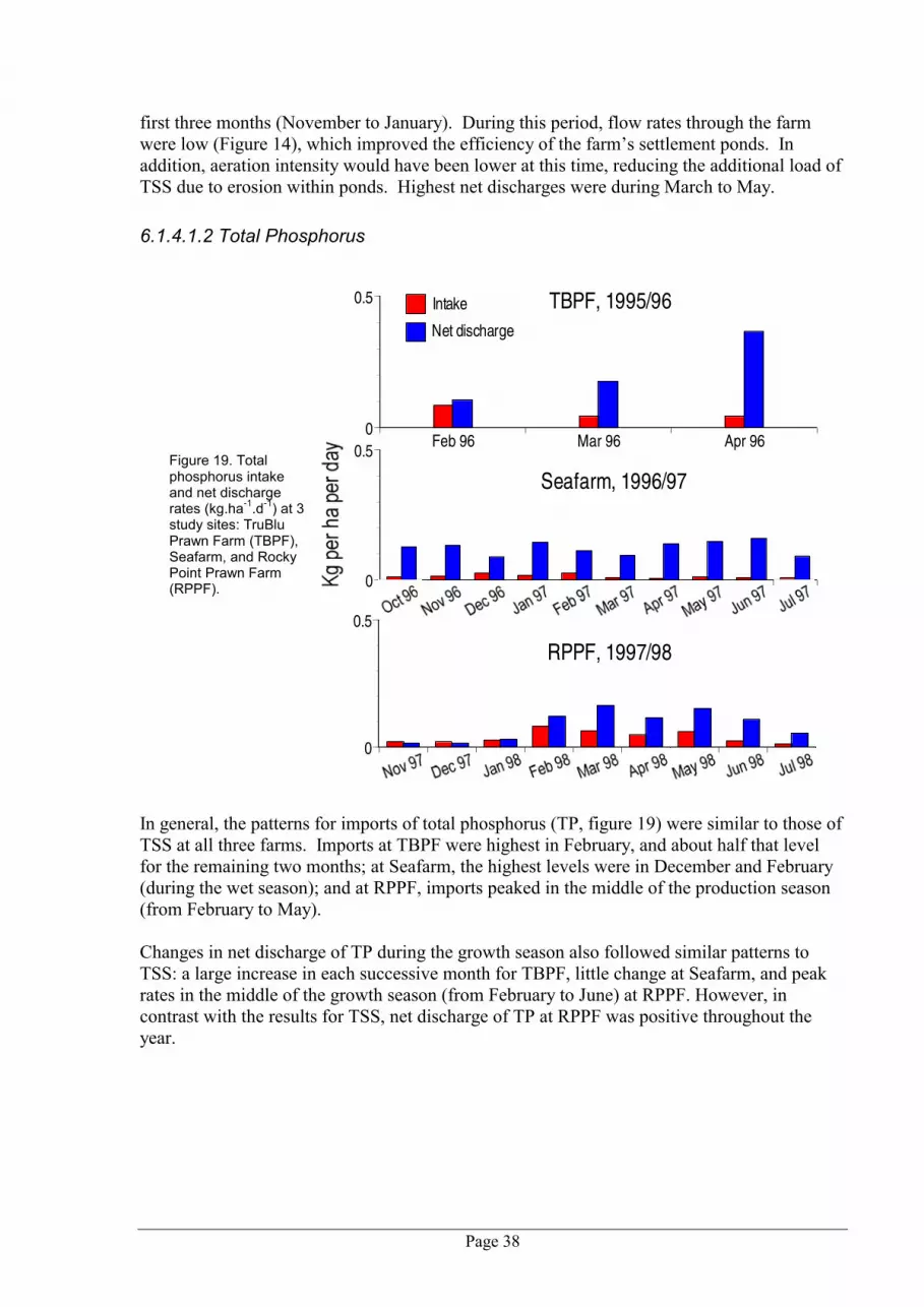
Page 38
first three months (November to January). During this period, flow rates through the farm were low (Figure 14), which improved the efficiency of the farm�s settlement ponds. In addition, aeration intensity would have been lower at this time, reducing the additional load of TSS due to erosion within ponds. Highest net discharges were during March to May. 6.1.4.1.2 Total Phosphorus Figure 19. Total
phosphorus intake and net discharge rates (kg.ha-1.d-1) at 3 study sites: TruBlu Prawn Farm (TBPF), Seafarm, and Rocky Point Prawn Farm (RPPF).
In general, the patterns for imports of total phosphorus (TP, figure 19) were similar to those of TSS at all three farms. Imports at TBPF were highest in February, and about half that level for the remaining two months; at Seafarm, the highest levels were in December and February (during the wet season); and at RPPF, imports peaked in the middle of the production season (from February to May). Changes in net discharge of TP during the growth season also followed similar patterns to TSS: a large increase in each successive month for TBPF, little change at Seafarm, and peak rates in the middle of the growth season (from February to June) at RPPF. However, in contrast with the results for TSS, net discharge of TP at RPPF was positive throughout the year.
Feb 96 Mar 96 Apr 960
0.5 TPINPHAPD
TPNETPHAPD
Intake
Net discharge
0
0.5
TBPF, 1995/96
Seafarm, 1996/97
0
0.5
RPPF, 1997/98

Page 39
6.1.4.1.3 Total Nitrogen Figure 20. Total
nitrogen intake and net discharge rates (kg.ha-1.d-1) at 3 study sites: TruBlu Prawn Farm (TBPF), Seafarm, and Rocky Point Prawn Farm (RPPF).
For TN (total nitrogen, figure 20), the seasonal comparison between the three farms was similar to the other nutrients. At TBPF, net discharge rates again increased each month, from 1.4 kg.ha-1.d-1 in February to 2.4 kg.ha-1.d-1 in April. However although (as for the other nutrients) the highest import rate of TN occurred in February, imports in subsequent months were not much lower. At Seafarm, imports of TN paralleled imports of TSS: the highest rates were from October to December, with little variation during the rest of the season. Net discharge of TN showed no clear seasonal pattern. At RPPF, in contrast to the other nutrients, TN imports were not substantially lower for the first three months; and the highest import rate (1.1 kg.ha-1.d-1) was in May. However the pattern of net export, with peak rates from February to June, was similar to the other nutrients.
Feb 96 Mar 96 Apr 960
1
2TNINPHAPD
TNNETPHAPD
Intake
Net discharge
0
1
2
TBPF, 1995/96
Seafarm, 1996/97
0
1
2 RPPF, 1997/98

Page 40
6.1.4.2 Overall budget characteristics To characterise the nutrient imports and net discharges at each farm, all calculated rates were averaged over the whole of each respective study period, for each farm (Figure 21). Figure 21. Whole-season
average intake and net discharge rates (kg.ha-1.d-1) for 3 nutrients: total suspended solids (TSS), total phosphorus (TP), and total nitrogen (TN). TBPF, TruBlu Prawn Farm; RPPF, Rocky Point Prawn Farm.
6.1.4.2.1 TruBlu Prawn Farm TBPF had, by far, the highest import rate for TSS (average 84 kg.ha-1.d-1, compared to less than 20 kg.ha-1.d-1 at the other two farms). This is a result of the farm�s location on the lower reaches of the Clarence River: a major river system, with a large catchment (22,700 km2, the largest catchment on the NSW coastline), frequently carrying a high load of particulate matter. In addition, the TBPF pump intakes are deliberately located close to the river bottom, to maximise the probability of accessing high salinity water during periods of heavy rainfall and high river flow. However this arrangement probably exacerbated the high TSS levels in farm intake water. The high net discharge of TSS at TBPF (87 kg.ha-1.d-1, compared to 30 kg.ha-1.d-1 at Seafarm, and only 4 kg.ha-1.d-1 at RPPF) was due to erosion, both within the ponds (due to aeration currents) and within the narrow discharge channels. Erosion effects were particularly evident at this farm due to the combination of a light, loamy soil structure with high water exchange rates (despite the much smaller area of TBPF compared to Seafarm, the water usage is similar � see Figures 3 and 7). TBPF also had the highest net discharges of TP and TN. This was due largely to less efficient feed utilisation, caused by a number of factors including low salinity for much of the year, frequent disease problems, and lack of experience with Penaeus japonicus (this was the first year the farm had cultured this more difficult species). 6.1.4.2.2 Seafarm Seafarm was characterised by having the lowest imports of TSS, TP and TN. Low intake loads of TSS are consistent with the low tidal currents, small catchment, and lack of upstream
0
50
100AVINTSS
AVNETTSS
TSS
0
0.1
0.2TP
TBPF Seafarm RPPF0
0.5
1
1.5
2TN
Intake
Net discharge

Page 41
agriculture of the mangrove creek upon which the farm�s intake was situated. In general, the low import rates at Seafarm reflect the fact that the supply water had a lower nutrient load than at the other two farms. The net discharge rates of TSS, TP and TN at Seafarm were lower than TBPF but higher than RPPF � although in the case of TN, the difference was marginal (1.0 kg.ha-1.d-1 at Seafarm, 0.9 kg.ha-1.d-1 at RPPF). 6.1.4.2.3 Rocky Point Prawn Farm The import of TN at RPPF (0.52 kg.ha-1.d-1) was the highest of the three farms studied. The import rate for TP(0.04 kg.ha-1.d-1) was also high, although not quite as high as at TBPF. The high levels of nutrients in the RPPF intake water is probably due fertiliser runoff as the intake canal passes through sugar cane fields. However the net TSS discharge was by far the lowest of all farms, averaging only 3.7 kg.ha-1.d-1 over the study period. We attribute this extremely low net TSS discharge rate at RPPF to settlement of particulate matter, both in treatment ponds within the farm and during the time taken for the discharge water to reach the sampling location 400 m away from the farm (Figure 4, Methods). Net discharge rates for TN and TP were also the lowest of all three farms studied, probably due to the effects of the treatment ponds.

Page 42
6.2 Discharge components The composition of the discharge water was studied during two intensive sampling periods at Seafarm: in Feb and July/Aug 1997. Three samples were taken each day.
6.2.1 Discharge nutrients Figure 22. Nutrients in
Seafarm discharge during two intensive 1-week sampling periods in 1997. Three samples were taken each day. A, February; B, July/August.
There was substantial variation in chlorophyll a levels, even for samples taken only a few hours apart. For example on 21/2/97, chlorophyll a dropped from over 100 µg.L-1 to about 20 µg.L-1 in consecutive samples (Figure 22 A); and on 3/8/97 two samples of about 40 µg.L-1 were followed by a sample with over 200 µg.L-1 (Figure 22 A). The total P and N values also exhibited large changes within a few hours.
0
100
200 Chlorophyll (ug/l)
0.0
0.2
0.4 Total P (mg/l)
19/2/1997 20/2/1997 21/2/1997 22/2/1997 23/2/1997 24/2/1997 25/2/19970123 Total N (mg/l)
A
0
100
200 Chlorophyll (ug/l)
0.0
0.2
0.4 Total P (mg/l)
29/7/1997 30/7/1997 31/7/1997 1/8/1997 2/8/1997 3/8/1997 4/8/19970123 Total N (mg/l)
B

Page 43
6.2.2 Discharge nitrogen components Figure 23. Discharge N components, Seafarm, 1997. NH3 is total
ammoniacal nitrogen, TAN. During the intensive sampling period in February, 38.2% of the N in the discharge water at Seafarm was in the particulate fraction. 22.1% was TAN, while the remaining 39.7% was other dissolved forms of N (Figure 23). During the second intensive sampling period, in July to August, there was a lower proportion of TAN (only 11.8%); and both particulate and other dissolved fractions were correspondingly greater. However the proportion of N components was not consistent between samples. For example, ammonia levels varied considerably over short time frames. Despite the average ammonia proportion being higher during February than later in the year, some samples had very low or negligible ammonia levels, eg the 2nd and 3rd samples on 19/2/97, and the 2nd samples on 21/2/97 and 23/2/97.
19/2/1997 20/2/1997 21/2/1997 22/2/1997 23/2/1997 24/2/1997 25/2/19970.00.51.01.52.02.5
NH3Other dissParticulate
February
29/7/1997 30/7/1997 31/7/1997 1/8/1997 2/8/1997 3/8/1997 4/8/19970.00.51.01.52.02.5
AugustN (m
g/l)
22.1%39.7%
38.2%
11.8%43.6%
44.6%

Page 44
6.3 Effluent treatment
6.3.1 RPPF treatment ponds, 1997/98 season
6.3.1.1 Water flow through the treatment ponds The flow through the treatment ponds varied considerably from day to day. Results during the two sampling periods are shown. The average flow rate during the first sampling period, 27/1/98 to 4/2/98, was 0.052 megalitres (ML) per hour (Figure 24). During the second sampling period, 21/3/98 to 27/3/98, the average flow rate was 0.049 ML.h-1 (Figure 25).
Figure 24. Water flow through treatment ponds during first sampling period (27/1/98 to 4/2/98)
Figure 25. Water flow through treatment ponds during the second sampling period (21/3/98 to 27/3/98)
6.3.1.2 Changes in nitrogen concentration within treatment ponds Over both sampling periods, there was a consistent reduction in total N concentration of between 11 and 40% as the water passed through the treatment pond system (mean value, 20.3%: Figure 26). Most of this reduction in N concentrations occurred within the first pond (that is, between the ‘Intake’ and ‘Middle’ samples).
Figure 26. Total nitrogen (TN) levels during two intensive sampling periods. INTAKE, samples from beginning of settlement pond (sampling point A); MIDDLE, samples from end of settlement pond (sampling point B); DISCHARGE, samples from end of aquatic-plants pond (sampling point C).
ML/h
ML/h
27/01/98
28/01/98
29/01/98
30/01/98
31/01/98
01/02/98
02/02/98
03/02/98
04/02/98
05/02/98012345
TN (m
g/l) INTAKE
MIDDLEDISCHARGE
21/03/98
22/03/98
23/03/98
24/03/98
25/03/98
26/03/98
27/03/98012345
TN (m
g/l)

Page 45
6.3.1.3 Nitrogen reduction performance of treatment ponds The nitrogen reduction performance of the treatment ponds is calculated taking into account the pond area, and the flow rate of water through the pond. The steps leading to the final result are shown in Table 1. The water flow rate is multiplied by the incoming N concentration to calculate mass of N delivered to the treatment pond, in kg.d-1; similarly, the mass of N discharged from the pond is calculated from the discharge concentration and flow rate. The difference between N input and N discharged is the N removal rate (in kg.d-1); this is then divided by the treatment pond area to generate N removal in kg.ha-1.d-1.
The calculations for the four sets of results (two types of treatment pond, each sampled on two occasions) are exactly the same. The data for nitrogen concentration on input and discharge, and the flow rates through the ponds, are averaged over each of the two sampling periods.
Settlement pond (0.372 ha)
Aquatic-plants pond (0.118 ha)
January 1998
March 1998
January 1998
March 1998
Flow rate (ML/d)
1.25 1.18 1.25 1.18
Average N in (mg/L)
3.62 3.56 3.00 3.04
Daily N in (kg)
4.52 4.19 3.73 3.57
Average N out (mg/L)
3.00 3.04 2.76 2.85
Daily N out (kg)
3.73 3.57 3.45 3.35
N reduction (kg/d)
0.79 0.62 0.29 0.23
N reduction (kg/ha/d)
2.12 1.66 2.41 1.90
Table 1. Calculation of N removal capacity in the treatment pond at Rocky Pt Prawn Farm.
The source of data and calculations are:
Flow rate (ML.d -1): The average flow through the treatment pond system, from Figures 24 and 25.

Page 46
Average N in (mg.L-1): For the settlement pond, this is the daily INTAKE figures averaged from Figure 26. For the aquatic-plants pond, MIDDLE figures are averaged.
Daily N intake (kg): (Flow rate) x (Average N in)
Average N outlet (mg.L-1): For the settlement pond, this is the daily MIDDLE figures averaged from Figure 26. For the aquatic-plants pond, DISCHARGE figures are averaged.
Daily N outlet (kg): (Flow rate) x (Average N out)
N reduction (kg.d-1): (Daily N in) – (Daily N out)
N reduction (kg.ha-1.d-1): (N reduction kg.d-1) / (treatment pond area)
Therefore, at different times the two different styles of treatment ponds removed between 1.66 and 2.41 kg of N, per ha of treatment pond, per day (Figure 27).
6.3.1.4 Comparison of RPPF treatment pond types In the initial design of the treatment system, the two ponds were intended to have complementary functions. However in practice, their modes of operation became blurred. For example, considerable quantities of aquatic plants grew in the first pond as well as the second; and our data showed that, at times, substantial quantities of particulate matter settled out in the second pond as well as the first. Although stakes and mesh panels were placed in the first pond to encourage colonisation by filter-feeders such as tube-worms and barnacles, in fact there was relatively little recruitment of these organisms. On the other hand, large numbers of insect larvae (eg, midges) colonised both ponds, and their metamorphosis (and airborne departure) probably represented an unplanned but effective removal of N from the system.
Because the processes involved in the two ponds remain poorly understood, we have not assumed any functional links between them; we simply treat the results from the two ponds as independent estimates of nitrogen-reduction performance from two different examples of pond design.
Figure 27. Nitrogen reduction (kgN/ha/d) for two treatment ponds (Passive and Algae) early (January) and later in the production season (March).
Passive Algae0.0
1.0
2.0
3.0
kgN
/ha/
day
JanuaryMarch
Nitrogen reduction

Page 47
While the four N removal-rate estimates are similar, there are some consistent differences which shed some light on both the processes occurring in the ponds, and how the treatment systems might be expected to perform over an extended period.
Firstly, the ‘Algae’ pond was more efficient at removing N than the ‘Passive’ settlement pond: in both January and March 1998, the algae pond removed about 14 to 15% more N than the passive pond – undoubtedly because some N was taken up by the plant growth (Figure 27). However, this improved performance came at a cost: aquatic plants needed to be physically harvested from the pond every few weeks, a difficult and labour-intensive task. Also, the plant growth was somewhat unpredictable, and the dominant species varied throughout the season. The plant species that predominated early in the season was rooted, and particularly difficult to harvest.
Secondly, the performance of both types of ponds was lower during the second sampling period during late March 1998. Nitrogen removal rates were about 20% lower. Other studies (below) have suggested that over time, some of the organic matter which had settled to the bottom began to decompose, thus remineralising nitrogen, mainly in the form of ammonia. This process will lead to the reduced efficiency of N removal, in both types of treatment pond, over time.
6.3.2 Gold Coast Marine Prawn Farm, 1997/98 season
Figure 28. Changes in water quality in GCMPF treatment pond during the 1997/98 season � all results in mg.L-1. See Figure 7, Methods, for sampling locations. TSS, total suspended solids; TPO, total particulate organics; TN, total nitrogen; DN, dissolved nitrogen; NH3, total ammonia nitrogen; NOx, nitrogen oxides (NO3 + NO2).
23/12/1997 20/1/1998 24/2/1998 31/3/19980
20
40
IntakeMiddleDischarge
TSS
23/12/1997 20/1/1998 24/2/1998 31/3/19980
10
20 TPO
23/12/1997 20/1/1998 24/2/1998 31/3/19980
1
2 TN
23/12/1997 20/1/1998 24/2/1998 31/3/19980
1
2 DN
23/12/1997 20/1/1998 24/2/1998 31/3/19980
1
2 NH3
23/12/1997 20/1/1998 24/2/1998 31/3/19980
1
2 NOx

Page 48
Water samples were taken on four occasions during the season: in December 1997, and in January, February and March 1998. TSS and TPO were reduced significantly in the settlement basin: TSS in the Middle samples was only between 23 and 62% of that at the Intake, while TPO was reduced to between 31 and 62% of the Intake level (Figure 28). These reductions in the particulate matter occurred throughout the season. However, the results for Nitrogen were less consistent. Total Nitrogen decreased in the settlement zone during the first two sampling periods (reduced to 70 and 76%); however, on the third sampling occasion (February) there was no change; and on the final occasion (March) the concentration of total Nitrogen actually increased by 7% (TN, Figure 28). The second part of the treatment system (the �structure zone�) had little effect on discharge water quality (ie there was no consistent difference between the Middle and Discharge samples, Figure 28). This was probably due, at least in part, to its small area � only 0.226 ha, compared to 0.809 ha for the settlement basin. Examining data for the Nitrogen components indicates what was occurring. There was little change in Dissolved Nitrogen between the Intake and Middle samples during December or January (Figure 28), implying that the reduction in total N which occurred during these months was due to particulate organic matter being removed from the water column. However, during February and March, the concentration of Dissolved Nitrogen increased substantially (by about 50%) between the Intake and Middle samples. We suggest this was due to decomposition of the accumulated organic matter in the sediments. A study conducted by the CRC for Aquaculture in this pond which measured benthic fluxes from the sediment, found high flux rates of TAN from the sediment where particulate matter had accumulated (M. Burford, unpublished data). While some of the increase can be accounted for in the dissolved inorganic components (NH3 and NOx), there must also have been a substantial increase in dissolved organic Nitrogen. 6.3.2.1 Growth of biota in the treatment system The large settlement basin did not support significant populations of filter-feeders or other biota. Whenever sediment cores were taken, or sediment traps were deployed, a qualitative assessment was made of any benthic or epibenthic fauna present; such biota were rarely observed. This was a notable contrast to the situation observed in the other treatment systems studied in this project. We suggest the lack of benthic fauna may have been due to the high benthic loading of settled particulate matter. It is also possible that the high flow-rate through the large settlement basin prevented the establishment of benthic fauna. However, large beds of bivalves settled on rock structures near the Middle sampling location (Figure 7, Methods) and on the physical structures installed within the Structure zone (Figure 8, Methods). In these areas the currents were generally stronger than 1 m.s-1.
6.3.3 Gold Coast Marine Prawn Farm, 1998/99 season Our initial studies of treatment systems (at RPPF and GCMPF during 1997/98) indicted high rates of N remineralisation from the organic matter in the sediment. Accordingly, we designed an experiment to test the hypothesis that the removal of accumulated sediment from the pond would reduce N remineralisation rates. In order to ensure complete removal of accumulated sediment, and to eliminate possible leaching of nutrients from original soil

Page 49
substrate, the experimental treatment pond constructed for this project was fully lined with polyethylene sheet. Our initial intention was to construct an experimental treatment pond system with the same relative flow rate (L.s-1.ha-1) as the main treatment facility studied the previous year. On this basis, the pond (total area 1030m2) should have had a flow rate of 28 L.s-1. However, the flow rate which was eventually actually achieved was only 12 L.s-1 (1.04 ML.d-1), due to the limited pumping capacity available. Therefore the two systems are not directly comparable. 6.3.3.1 Pond operation The treatment pond began operation on 27/12/98. It was drained and cleaned on two occasions: 3/2/99 (after 6 weeks operation) and when the study was completed, on 15/4/99 (after a further 8 weeks). The pond was cleaned manually: the water was first pumped out and then remaining sludge removed by hosing, sweeping and using a sludge pump (right). 3 workers took approximately ¾ of a day to complete each cleaning.
6.3.3.2 Sampling and analysis Water samples were collected (3 replicates each from inlet and outlet), once per week from 7/1/99 to 6/4/99. The samples were analysed for both particulate and dissolved nutrients � with particular emphasis on nitrogen. The suspended solids were measured and divided into inorganic and organic components; Chla was also determined. Each time the system was drained, sediment depth was measured and sediment samples were collected to be analysed for TN, TP, organic content, moisture and density. 6.3.3.3 Results
6.3.3.3.1 Growth of biota and effects of first cleanout During the first cleanout (on 3 Feb 99) the following organisms were observed in the sediment and attached to solid structures: barnacles, tube worms, chironomid worms, bivalves, sergestids, bloodworms, and prawns (Figure 29). In addition, large quantities of filamentous algae began growing around the pond walls after the first few weeks. However the drying associated with the February cleanout clearly had a negative impact on these populations; substantially fewer organisms were seen for the remainder of the study � although the filamentous algae did re-colonise some weeks after the cleanout.
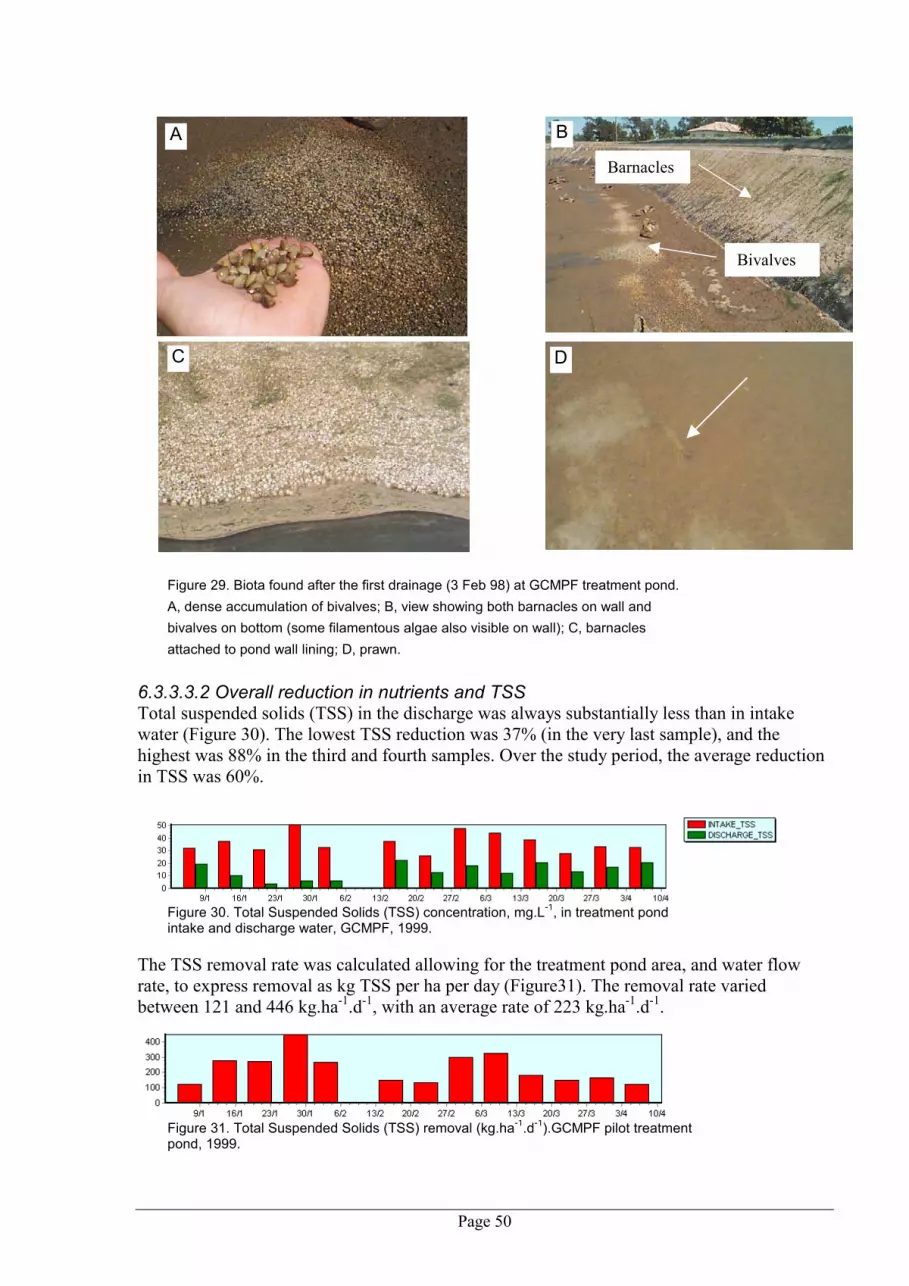
Page 50
Figure 29. Biota found after the first drainage (3 Feb 98) at GCMPF treatment pond. A, dense accumulation of bivalves; B, view showing both barnacles on wall and bivalves on bottom (some filamentous algae also visible on wall); C, barnacles attached to pond wall lining; D, prawn.
6.3.3.3.2 Overall reduction in nutrients and TSS Total suspended solids (TSS) in the discharge was always substantially less than in intake water (Figure 30). The lowest TSS reduction was 37% (in the very last sample), and the highest was 88% in the third and fourth samples. Over the study period, the average reduction in TSS was 60%.
Figure 30. Total Suspended Solids (TSS) concentration, mg.L-1, in treatment pond intake and discharge water, GCMPF, 1999.
The TSS removal rate was calculated allowing for the treatment pond area, and water flow rate, to express removal as kg TSS per ha per day (Figure31). The removal rate varied between 121 and 446 kg.ha-1.d-1, with an average rate of 223 kg.ha-1.d-1.
Figure 31. Total Suspended Solids (TSS) removal (kg.ha-1.d-1).GCMPF pilot treatment pond, 1999.
A B
C D
Barnacles
Bivalves

Page 51
Concentrations of TP followed a similar pattern to that of TSS. Except for the last sample, discharge concentration was lower than intake; this was particularly pronounced for the first five sampling times, before the Feb cleanout (Figure 32). During this period, reduction in TP varied between 28 and 67%. Over the study period, the average reduction in TP was 33%.
Figure 32. Total Phosphorus (TP) concentration, mg.L-1, in treatment pond intake and discharge water, GCMPF, 1999.
TP removal rates varied between �0.13 kg.ha-1.d-1 (for the last sample) and 1.48 kg.ha-1.d-1; the average rate was 0.73 kg.ha-1.d-1 (Figure 33).
Figure 33. Total Phosphorus (TP) removal (kg.ha-1.d-1), GCMPF pilot treatment pond, 1999.
Total Nitrogen concentrations were reduced quite consistently; the average reduction was 21%, and the range was from 10% to 34% (Figure 34).
Figure 34. Total Nitrogen (TN) concentration, mg.L-1, in treatment pond intake and discharge water, GCMPF, 1999.
Calculated in terms of mass of N removed, the treatment pond removed between 2.9 and 10 kg N.ha-1.d-1, with an average rate of 5.7 kg N.ha-1.d-1 (Figure 35). There was no systematic change in removal rate during the course of the study. The GCMPF pilot treatment pond therefore was far more effective than either the deep or shallow pond at RPPF, which removed only 1.6 to 2.4 kg N.ha-1.d-1.
Figure 35. Total Nitrogen (TN) removal (kg.ha-1.d-1), GCMPF pilot treatment pond, 1999.
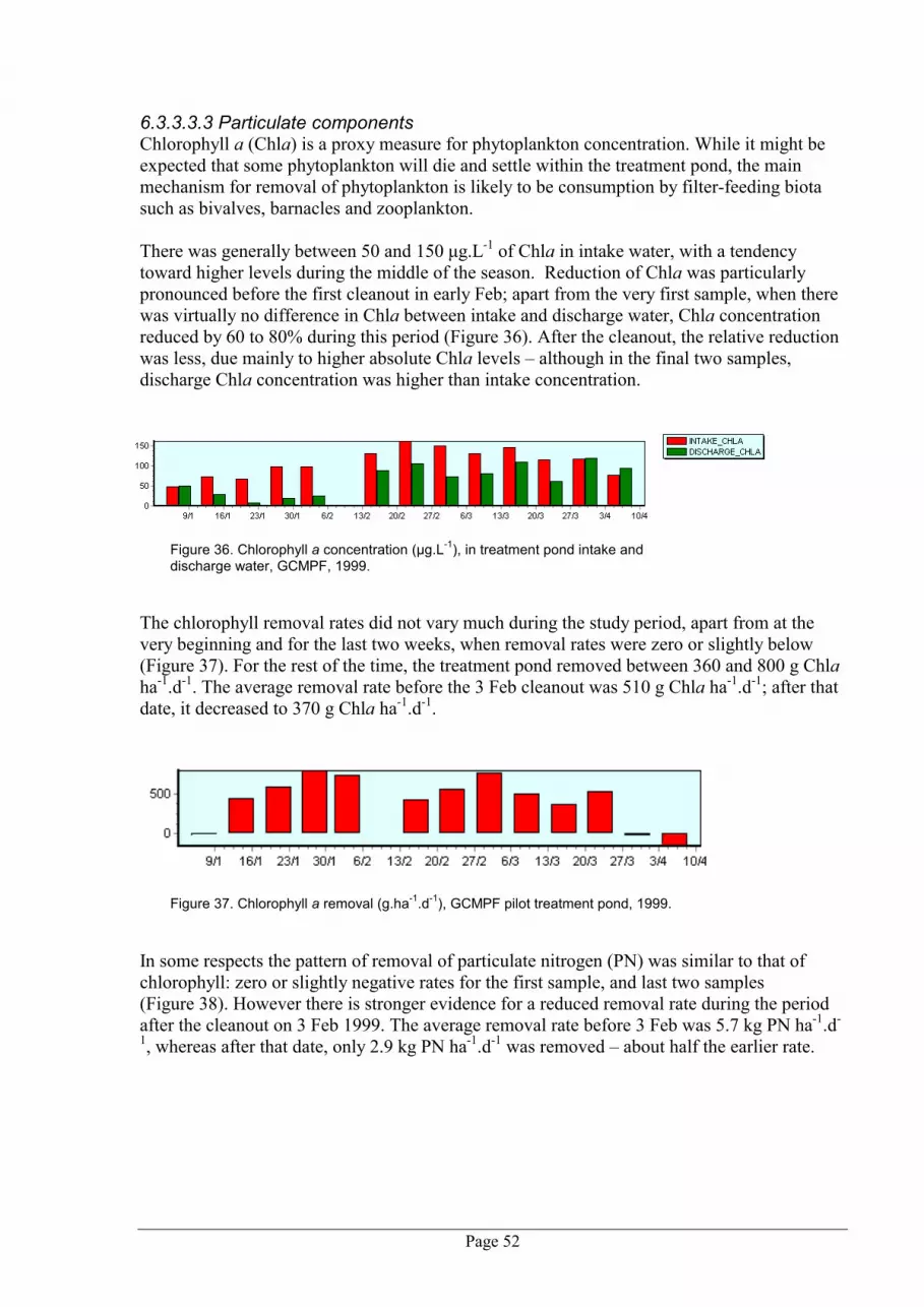
Page 52
6.3.3.3.3 Particulate components Chlorophyll a (Chla) is a proxy measure for phytoplankton concentration. While it might be expected that some phytoplankton will die and settle within the treatment pond, the main mechanism for removal of phytoplankton is likely to be consumption by filter-feeding biota such as bivalves, barnacles and zooplankton. There was generally between 50 and 150 µg.L-1 of Chla in intake water, with a tendency toward higher levels during the middle of the season. Reduction of Chla was particularly pronounced before the first cleanout in early Feb; apart from the very first sample, when there was virtually no difference in Chla between intake and discharge water, Chla concentration reduced by 60 to 80% during this period (Figure 36). After the cleanout, the relative reduction was less, due mainly to higher absolute Chla levels � although in the final two samples, discharge Chla concentration was higher than intake concentration.
Figure 36. Chlorophyll a concentration (µg.L-1), in treatment pond intake and discharge water, GCMPF, 1999.
The chlorophyll removal rates did not vary much during the study period, apart from at the very beginning and for the last two weeks, when removal rates were zero or slightly below (Figure 37). For the rest of the time, the treatment pond removed between 360 and 800 g Chla ha-1.d-1. The average removal rate before the 3 Feb cleanout was 510 g Chla ha-1.d-1; after that date, it decreased to 370 g Chla ha-1.d-1.
Figure 37. Chlorophyll a removal (g.ha-1.d-1), GCMPF pilot treatment pond, 1999.
In some respects the pattern of removal of particulate nitrogen (PN) was similar to that of chlorophyll: zero or slightly negative rates for the first sample, and last two samples (Figure 38). However there is stronger evidence for a reduced removal rate during the period after the cleanout on 3 Feb 1999. The average removal rate before 3 Feb was 5.7 kg PN ha-1.d-
1, whereas after that date, only 2.9 kg PN ha-1.d-1 was removed � about half the earlier rate.

Page 53
Figure 38. Particulate N removal (kg.ha-1.d-1), GCMPF pilot treatment pond, 1999.
While chlorophyll a is strictly a measure of phytoplankton density, particulate nitrogen can also include non-phytoplankton protein sources. These could include uneaten food, bacteria, detritus, faecal fragments and zooplankton. However, a complementary study by the CRC for Aquaculture showed that most of the particulate N (60-80%) in prawn ponds was phytoplankton (M. Burford, unpublished data). The data suggest that these non-phytoplankton particulates were being removed far less efficiently during the last few weeks of the experiment. Comparing the removal rates for particulate nitrogen and dissolved nitrogen (DN) reveals that, before the 3 Feb cleanout, removal of PN was by far the dominant process, particularly after the first two sampling times: between 7.5 and 10 kg.ha-1.d-1 were removed, while DN removal was negligible or negative for most of this period (Figure 39). However after 3 Feb, this situation reversed to an extent. As already noted, the removal rate for PN was substantially lower during the last few weeks. Removal of DN, on the other hand, increased considerably during this period, and was the dominant process in five of the eight samples taken.
Figure 39. Comparison between removal rates (kg.ha-1.d-1) of dissolved and particulate nitrogen, GCMPF pilot treatment pond, 1999.
This is a different outcome from the previous year, where there was a clear net increase in DN concentration (ie, negative DN removal rate) after two months� operation. Therefore the objective of this study � to reduce emission of DN by removing settled organic matter � was achieved.
6.3.4 Summary: performance comparison of the treatment systems During this project, five different treatment ponds were studied (including the two pond sections at each of RPPF and GCMPF during 1997/98). These varied widely in area, flow rates, depth (Table 2), and composition of incoming water; and not surprisingly, performance varied also. To provide a meaningful comparison, each pond was characterised by the residence time of water flowing through it (calculated as the inverse of daily exchange rate: Table 2). The percent reduction in concentration of TSS, TP and TN was then examined.

Page 54
RPPF 97/98 GCMPF 97/98 GCMPF 98/99
Deep/ structure
Shallow/ plants
Main Structure
Reference (used below) RPPF1 RPPF2 GCM1 GCM2 GCM99
Area (ha) 0.372 0.118 0.803 0.226 0.103
Overflow rate (ML.d-1.ha-1) 3.2 10.21 26.9 95.6 10.1
Depth (m) 1.5 0.25 1.8 1.4 2.0
Exch.d-1 0.22 4.07 1.49 6.83 0.50
Residence time (d) 4.65 0.25 0.67 0.15 1.98
Table 2. Summarised characteristics of discharge treatment ponds studied during the project.
In the following discussions, codes are used to refer to each of the five ponds: RPPF1, RPPF2: stages 1(deep) and 2 (shallow) of RPPF treatment pond, studied during 1997/98; GCM1, GCM2: stages 1 (main) and 2 (structure) of GCMPF treatment pond, studied during 1997/98; GCM99: GCMPF pilot treatment pond, studied during 1999 (Table 2). 6.3.4.1 Total suspended solids (TSS)
Figure 40. Change in TSS within five treatment ponds. A, input (brown squares) and discharge (blue circle) TSS concentration (mg.L-1). B, percent reduction in TSS (concentration difference as a proportion of initial concentration): mean ± SE. See text and Table 2 for pond identification.
Input TSS concentrations for GCM1, GCM99 and RPPF1 were remarkably consistent, at around 35 � 40 mg.L-1 (Figure 40 A). Ponds GCM1 and GCM99 were both very effective at reducing TSS: concentrations were reduced by about 60% (Figure 40 B). These ponds had residence times of 0.7 and 2.0 d respectively. RPPF1, despite its much longer residence time (4.7 d) actually had less impact on TSS concentration, reducing it by only 39%. This may reflect different particle sizes of eroded particulate matter at the two farms, due to varying soil types, and resulting in different deposition rates. Alternatively, it may be that, given the extended residence time in RPPF1, once inorganic particulates had been removed (thus allowing greater light penetration) there was time for phytoplankton to increase in density, thereby replacing the inorganic TSS. Both the second-stage ponds (RPPF2 and GCM2) performed quite poorly in removing TSS, reducing concentration by only about 10%. This simply reflects the fact that in each case, the
B
B
B
B
B
010
2030405060
70
0 1 2 3 4 5Residence time (d)
RPPF 1
RPPF 2
GCM 1
GCM 2
GCM99B
B
B
B
B
JJ
JJ J
0
10
20
30
40
0 1 2 3 4 5Residence time (d)
RPPF 1
RPPF 2
GCM 1
GCM 2
GCM99A B

Page 55
preceding first-stage pond (RPPF1 and GCM1 respectively) had already removed most of the available TSS (Figure 40 A). Therefore, provided the residence time is 1 d or higher, maximum removal of TSS should be achieved. Longer residence times do not seem to result in lower TSS concentrations in discharge water. 6.3.4.2 Total phosphorus (TP)
Figure 41. Change in TP within five treatment ponds. A, input (brown squares) and discharge (blue circle) TP concentration (mg.L-1). B, percent reduction in TP (concentration difference as a proportion of initial concentration): mean ± SE. See text and Table 2 for pond identification.
Input levels of TP varied considerably, from about 0.15 mg.L-1 in GCM1 to about 0.4 mg.L-1 at RPPF1 (Figure 41 A). The high level at RPPF is probably due to a combination of the recirculation at that farm, and nutrients entering the intake water from cane farm runoff. The TP reduction in GCM1 and GCM2 was more variable than that in the other ponds (Figure 41 B). The main reason for this is the low number of observations during this study (only 4 compared with 13 at GCM99 and even more at RPPF1 and RPPF2). Because of the variability, results for GCM1 and GCM2 must be considered less reliable. In most respects the results for TP were very similar to those for TSS. This is because much of the phosphorus in discharge water is either closely bound to inorganic particles, or contained in phytoplankton cells; therefore effectiveness in reducing in TSS is also likely to be reflected in TP removal. However in contrast to the TSS results, there does seem to be a significant benefit in extending residence time to at least two days: the TP concentration-reduction in GCM99 was significantly better than in those ponds with lower residence times (Figure 41 B). Another difference between the results for TSS and TP is that RPPF2 had a similar performance to RPPF1. This indicates that the high plant growth and plant harvesting in RPPF2 may have made a substantial contribution to TP removal.
BB
BB
B
JJ
JJ J
0.0
0.1
0.2
0.3
0.4
0.0 1.0 2.0 3.0 4.0 5.0Residence time (d)
RPPF 1
RPPF 2
GCM 1
GCM 2
GCM99
BB
B
B
B
05
10152025303540
0 1 2 3 4 5Residence time (d)
RPPF 1RPPF 2
GCM 1
GCM 2
GCM99BA

Page 56
6.3.4.3 Total Nitrogen (TN)
Figure 42. Change in TN within five treatment ponds. A, input (brown squares) and discharge (blue circle) TN concentration (mg.L-1). B, percent reduction in TN (concentration difference as a proportion of initial concentration): mean ± SE. See text and Table 2 for pond identification. GCM2 in B is off scale (-12%).
Input TN concentration was between 2 and 3 mg.L-1 for all ponds except RPPF1; similarly to TP, input concentration of TN to RPPF1 was slightly higher than the other ponds (about 3.5 mg.L-1: Figure 42 A). GCM99 was the most effective at reducing TN concentration, with an average reduction of 21%; RPPF1, reducing TN by 16%, had a similar effectiveness (Figure 42 B). While the reduction in TSS and TP in RPPF1 was much lower than in GCM99, the difference was smaller for TN. This is an indication that the optimal retention time for TN removal is probably longer than for the other two contaminants. This reflects the complex nature of nitrogen transformations within a treatment pond. While removal of TSS and (to a lesser degree) TP are mainly physical processes driven by settlement of particulates, nitrogen is involved in several pathways. These include conversion from organic matter to ammonia, uptake of ammonia by phytoplankton or other plants, conversion of ammonia to nitrite and nitrate (nitrification), settlement of nitrogen-containing particulates, consumption of phytoplankton by filter-feeding animals, and conversion of nitrate to molecular (gaseous) nitrogen (denitrification). The latter three of these processes can result in removal of nitrogen from the discharge water. Because of the complexity and interdependence of these transformations, it is not surprising that extended in-pond residence times result in greater reductions in nitrogen concentration. 6.3.4.4 Percent treatment area and retention time Two different measures of farm treatment capacity are commonly used: the percent pond area (in relation to total production area) and treatment pond retention time. The relationship between these two depends on depth of both treatment and production ponds, exchange rate during production, and frequency of pond drainage. Some examples have been calculated which assume production ponds are 1.5 m deep, and that 5% of total water volume is exchanged every day (Figure 43). If the treatment pond is 1.8 m deep, then 10% of the farm area devoted to treatment would correspond to a retention time of about 2.8 d (A, Figure 43); increasing the treatment area to 25% would increase the retention time to 8 d (B, Figure 43).
B
B
BB
B JJ
JJ J
0
1
2
3
4
0 1 2 3 4 5Residence time (d)
RPPF 1
RPPF 2
GCM 1
GCM 2
GCM99B
B
B
B
0
5
10
15
20
25
0 1 2 3 4 5Residence time (d)
RPPF 1
RPPF 2
GCM 1
GCM99BA

Page 57
However, the extra water volume discharged when a pond is drained for harvest needs to be allowed for. In a small farm, say 20 ha of production ponds, this would account for an extra 5% in discharge volume, reducing the previous 8 d retention time to 4 d (C, Figure 43). In a larger farm, say 50 ha, a single pond drainage would have a smaller incremental effect and would therefore only decrease the retention time to about 5.8 d (D, Figure 43). If the treatment ponds were only 1.5 m deep, the retention times would be correspondingly reduced (broken lines, Figure 43).
Figure 43. Relationship between treatment area (percent of total area) and treatment pond retention time (d). Solid lines: treatment ponds 1.8 m deep. Broken lines: treatment ponds 1.5 m deep. Exchange model reflects different scenarios for impact of full-pond drainage � see text for details. Assumptions: production ponds 1.5 m deep; constant daily exchange 5% of production volume.
In addition, if a farm operates seasonally it is normal for overall exchange rates to be very low (or zero) at the beginning of the season, and increase to higher levels toward the end � when both prawn biomass and water temperatures are higher. In this situation, the treatment pond retention time will steadily reduce through the season. 6.3.4.5 How much treatment area should be used? There is no easy answer to this question. The need for discharge treatment depends on factors such as the environmental values of a farm�s surroundings; other local industries impacting the environment; the size, design and management of the farm; and legislatory requirements. In addition, the design and management of the treatment system will determine how effectively it will perform at removing nutrients. However the results of our research can now provide some guidelines. Firstly, even quite a small treatment pond, with a retention time of one day or less, will be quite effective at removing TSS from the discharge stream. TSS levels will be reduced by about 60% (that is, reduced to 40% of pre-treatment TSS concentration). A 1 d retention time corresponds to about 5 to 10% of total farm area (Figure 43). Small ponds will, however, be less effective in removing nutrients (TP and TN). Our data suggest that a retention time of 2 to 3 d is required to significantly reduce concentrations; TP
0
2
4
6
8
10
12
0 5 10 15 20 25 30Percent treatment (of total)
normal
normal +2%
normal +5%
1.5 m1.8 m
Treatment pond depthExchange model
A
B
D C

Page 58
may be reduced by up to 35%, while TN should be reduced by 15 to 25%. A 3 d retention time corresponds to about 10 to 25% of farm area (Figure 43). 6.3.4.6 Improving nutrient removal performance Apart from physical settlement of inorganic particulates, a number of processes contribute to the removal of nutrients (N and P) in treatment ponds. Reducing nutrient levels beyond those already demonstrated will require more sophisticated design and management of treatment ponds, with a view to maximising as many of these processes as possible. Nutrient-removal processes include: • Physical settlement of organic matter: uneaten food, prawn faeces and moults,
phytoplankton, and zooplankton. However this process is of limited benefit because bacterial action in the sediment will mineralise nutrients contained in this organic matter, resulting in the nutrients being returned to the water in dissolved form (as was evident in RPPF1, RPPF2 and GCM1). Direct measurement of NH3 fluxes from the sediment in the GCM1 treatment pond indicate up to 3.8 kg N ha-1.d-1 was being released from the sediment as ammonia (M.A. Burford, unpublished data). The effectiveness of physical settlement as a N-removal process will therefore be improved by regularly removing settled deposits (as was done in GCM99) for land-based storage and treatment. However removal should be through pumping rather than draining the pond, so as not to disturb beneficial pond biota (see below: Incorporation into animal biomass)
• Denitrification: this is a bacterial conversion of NO3 (nitrate) to N2 (molecular nitrogen), subsequently dissipated to the atmosphere. This, together with commercial recovery (see below) is the best possible destination for waste N since the end product is completely benign. Currently, denitrification efficiency in prawn ponds � and, presumably, treatment ponds � is very low (Burford, unpublished data). To promote denitrification, several conditions must be met: the availability of sufficient sites with appropriate redox potential, a source of organic carbon, adequate levels of nitrate, and lack of denitrification-inhibiting compounds. Further research is needed to gain a better understanding of how these factors limit denitrification in treatment ponds; this may allow the design of treatment systems with improved denitrification rates.
• Volatilisation of ammonia: Ammonia in seawater exists in two forms, NH3 and NH4+;
the proportion of each depends on a number of factors, the most important being pH. Only un-ionised ammonia (NH3) is volatilised. Ammonia volatilisation is therefore enhanced by high pH levels, and is also increased by aeration and wind. Gross et al. (1999) found volatilisation rates equivalent to about 0.25 to 0.5 kg N.ha-1.d-1 from experimental catfish ponds (freshwater, presumably unaerated) when TAN concentration was 1 mg.L-1. This suggests that volatilisation is probably a significant, although not major, contribution to loss of N from prawn treatment ponds.
• Incorporation into plant biomass: this strategy was attempted, with limited success, in RPPF1. High plant growth rate was achieved, but plant harvests were too infrequent. Improved management, and ponds designed specifically to facilitate plant harvest, should be able to improve the efficiency of this strategy. While the plants grown in RPPF1 were the result of natural recruitment and had limited commercial value, an attractive alternative is to deliberately seed and grow plants with commercial markets. For example the seaweed Gracileria, used in production of agar for food and pharmaceuticals, has been successfully grown in prawn farm effluent in Australia (Jones et al. 2001) and overseas. However, because plants contain low N levels, substantial quantities of plant material need to be removed. For example 1.3 tonnes (wet wt) of plant material removed from the RPPF treatment pond contained only 9.1 kg N.

Page 59
• Incorporation into animal biomass (for commercial recovery): the potential exists to deliberately cultivate valuable crops such as oysters (eg Jones & Preston 1999), fish or even prawns at low-densities, in appropriately designed and managed treatment ponds. Such systems have the potential to both recover some nutrients from the discharge water, and contribute to overall farm profitability.
• Incorporation into animal biomass (non-commercial): extensive populations of naturally-seeded biota developed in all the ponds studied. These were principally filter-feeders (eg bivalves, barnacles, tube-worms), deposit feeders (eg chironomid larvae), or fish (eg mullet). Even without deliberate harvesting, most of the nutrients contained in these organisms will be completely removed from the discharge stream and the marine environment: for example insect larvae metamorphose and fly away; and when the pond is drained at the end of the season, filter-feeders will die and be consumed by birds or other terrestrial carrion feeders. Fish, if not harvested, can return to the marine environment when the pond is drained.

Page 60
7. FURTHER DEVELOPMENT In the short term it is important that the results of this research be communicated to all stakeholders as effectively as possible. This process has commenced via series of regional workshops culminating in a final national workshop on the �Environmental Management of Shrimp Farming in Australia�, held in Brisbane in May 2000. Communication of the project results will continue via: scientific publications; publication of the final report of the National Workshop on the Environmental Management of Prawn Farming in Australia; industry workshops; and participation in a new initiative by the Standing Committee on Fisheries and Aquaculture (SCFA) to apply Environmentally Sustainable Development principles to the Australian prawn farming industry. The results of this study are currently being incorporated into the following policy documents and industry guidelines: • Queensland Environmental Protection Agency, Marine Aquaculture Licensing • Great Barrier Reef Marine Park Aquaculture Regulations 2000 • Australian Prawn Farmers Code of Practice • Australian Prawn Farmers R&D Plan • Environmental Management of Prawn Farming in Australia � National Workshop Report,
FRDC At the international level, the results of this research have been included as one of several country by country case histories of environmental management of prawn farms (Preston et al. 2001b). It is intended that these case histories will contribute to a new initiative to develop �good management practices and good institutional and legal arrangements for shrimp farming�, through a program supported by the United Nations Food and Agriculture Organisation (FAO); the Network of Aquaculture Centres in Asia Pacific (NACA); the World Bank (WB); and the World Wide Fund for Nature In Australia, decisions are currently being made about the most sustainable forms of primary industry in coastal areas in order to ensure the effective management of the environment. The results of our research on prawn pond effluent composition and treatment are contributing to the process of providing a solid scientific basis for ensuring that the prawn farming industry is well placed in the future to meet these challenges. However, there is considerable work to be done to ensure the sustainable development the industry. In particular, further investment into the development and implementation of integrated waste management has significant potential to improve the economic and environmental performance of the industry (Burford et al. 2001). Finally we advocate a more structured approach to aquaculture planning, including the use of Geographic Information and Decision Support Systems (GIS/DSS) to assess the economic, environmental and social impacts of different land use scenarios. If this approach is to succeed there is a need to use GIS/DSS technology to combine geographic, biological, hydrodynamic, economic and social parameters with modeling of carrying capacity under different land-use scenarios, including prawn farming. This approach, incorporating the results of the present study and the closely linked research on environmental impacts by AIMS (FRDC 97/212) and the University of Queensland (CRC E.1 Final Report), has considerable potential to reduce conflicts arising from unplanned aquaculture development.

Page 61
8. CONCLUSION The objectives of this study were to improve our knowledge about the origin and composition of prawn pond discharges and to assess potential options for reducing the levels of solid and dissolved wastes discharged from farms. It was anticipated that this information would provide industry, regulators and the broader community with a rigorous and quantitative basis for understanding and improving the environmental management of the industry. The results confirmed previous observations that untreated prawn pond discharges contain elevated levels of TSS, total nitrogen and total phosphorus compared to the intake. However, farms that used treatment ponds were able to significantly improve effluent water quality. Most of the TSS (60% to 90%) was inorganic. Parallel research (CRC for Aquaculture Project E.1) has shown that most of this comes from eroded material from the pond floor and banks. Most (90%) of the nitrogen enters production ponds via prawn feeds. Only 22% of the input nitrogen is converted to prawns. By far the largest proportion (57%) is contained in discharge water with 14% remaining in the sediment. Only 3% of input nitrogen was unaccounted for, we assumed this was lost through denitrification and volatalisation of ammonia. These results confirm previous observations that current prawn farming systems are inefficient at converting feed nutrients to prawn biomass (Briggs & Funge-Smith 1994). An important implication of these observations is that there is considerable potential to reduce nitrogen waste via improved feed formulation and feed management, with attendant benefits in reducing effluent nutrient levels and improving farm profitability. Almost all (> 90%) of the total phosphorus was in the particulate form (ie a component of the TSS). The sources of total phosphorus include feeds, faeces, phytoplankton and detritus. Our results demonstrated a high level of variation in effluent loads between farms and over short time periods. This variability adds considerable complexity to the task of setting discharge loads and in designing waste management systems to meet the required standards. The results of this study have, for the first time, provided sufficiently accurate data on prawn farm effluent to permit comparisons with other sources of nutrients and suspended solids discharged into the same receiving waters. The results have also provided a more scientifically rigorous basis for setting permissible discharge loads from prawn farms, and for assessing the accuracy of effluent sampling strategies. However, the most cost-effective means of accurately monitoring compliance to effluent standards has yet to be determined. One of the major achievements of this project has been to develop and assess the use of settlement ponds to treat pond effluent prior to recirculation into production ponds or discharge into adjacent waterways. The results of our trials showed that settlement ponds reduced the net TSS load by 60%, TP load by 30% and TN load by 20%. Although pond effluent treatment technology is at an early stage of development, settlement ponds are now being used to assist farmers to meet the effluent discharge standards set by regulators. A clear outcome of this project, and the associated environmental impacts studies by AIMS (FRDC 97/212) and the University of Queensland (CRC E.1 Final Report), is consensus on the benefits of using settlement ponds to reduce effluent loads of particulate nutrients and inorganic particles. However, our results revealed that settlement ponds were less effective in removing dissolved nutrients. There is a need for further research to develop more efficient means of reducing dissolved nutrient loads in prawn pond effluent.
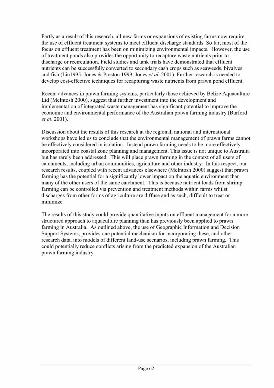
Page 62
Partly as a result of this research, all new farms or expansions of existing farms now require the use of effluent treatment systems to meet effluent discharge standards. So far, most of the focus on effluent treatment has been on minimizing environmental impacts. However, the use of treatment ponds also provides the opportunity to recapture waste nutrients prior to discharge or recirculation. Field studies and tank trials have demonstrated that effluent nutrients can be successfully converted to secondary cash crops such as seaweeds, bivalves and fish (Lin1995; Jones & Preston 1999, Jones et al. 2001). Further research is needed to develop cost-effective techniques for recapturing waste nutrients from prawn pond effluent. Recent advances in prawn farming systems, particularly those achieved by Belize Aquaculture Ltd (McIntosh 2000), suggest that further investment into the development and implementation of integrated waste management has significant potential to improve the economic and environmental performance of the Australian prawn farming industry (Burford et al. 2001). Discussion about the results of this research at the regional, national and international workshops have led us to conclude that the environmental management of prawn farms cannot be effectively considered in isolation. Instead prawn farming needs to be more effectively incorporated into coastal zone planning and management. This issue is not unique to Australia but has rarely been addressed. This will place prawn farming in the context of all users of catchments, including urban communities, agriculture and other industry. In this respect, our research results, coupled with recent advances elsewhere (McIntosh 2000) suggest that prawn farming has the potential for a significantly lower impact on the aquatic environment than many of the other users of the same catchment. This is because nutrient loads from shrimp farming can be controlled via prevention and treatment methods within farms whilst discharges from other forms of agriculture are diffuse and as such, difficult to treat or minimize. The results of this study could provide quantitative inputs on effluent management for a more structured approach to aquaculture planning than has previously been applied to prawn farming in Australia. As outlined above, the use of Geographic Information and Decision Support Systems, provides one potential mechanism for incorporating these, and other research data, into models of different land-use scenarios, including prawn farming. This could potentially reduce conflicts arising from the predicted expansion of the Australian prawn farming industry.

Page 63
9. REFERENCES APHA 1989. Standard Methods for the examination of Water and Wastewater. 17th Ed, American Public Health Association. APHA 1995. Standard Methods for the examination of Water and Wastewater. 19th Ed, American
Public Health Association. Briggs, M. R. P., Funge-Smith, S. J. 1994. A nutrient budget of some intensive marine shrimp ponds
in Thailand. Aquaculture and Fisheries Management 25:789-811. Burford, M.A. 1997. Phytoplankton dynamics in shrimp ponds. Aquaculture Research 28:351-360. Burford, M.A., Peterson, E.L., Baiano, J.C.F. and Preston, N.P. 1998. Bacteria in shrimp pond
sediments - their role in mineralising nutrients and some suggested sampling strategies. Aquaculture Research, 29: 135-140.
Burford, M.A., Jackson, C.J., Preston, N.P. 2001. Reducing nitrogen waste from shrimp farming � an integrated approach. In: Special Session of Shrimp Farming, World Aquaculture Society proceedings. (Eds.) Browdy, C. and Jory, D. In press.
Gross, A., Boyd, C.E., Wood, C.W. 1999. Ammonia volatilization from freshwater fish ponds. J. Environ. Qual. 28: 793-797.
Hobbie J.E., Daley R.J., Jasper S. 1977. Use of Nuclepore filters for counting bacteria by fluorescence miscroscopy. Applied Environmental Microbiology 33: 1225 � 1228.
Huguenin J.E., Colt J. (1989). Design and operating guide for aquaculture seawater systems. Developments in aquaculture and fisheries science, Vol 20, Elsevier NY. 264pp.
Jones, A.B. and Preston, N.P. 1999. Sydney rock oyster, Saccostrea commercialis (Iredale & Roughley), filtration of shrimp farm effluent: effects on water quality. Aquaculture Research, 30: 1-7.
Jones, A.B., Dennison, W.C., Preston N.P. 2001. Integrated treatment of shrimp effluent by sedimentation, oyster filtration and macroalgal absorption: a laboratory scale study. Aquaculture 193: 155-178
Lin, C.K. 1995. Progression of intensive marine shrimp culture in Thailand. pp. 13-23 In: C.L. Bowdy and J.S. Hopkins, editors. Swimming through troubled waters, Proceedings of the special session on shrimp farming, Aquaculture �95. World Aquaculture Society, Baton Rouge, Louisiana, USA
MacArthur Consulting Pty Ltd. 1995. Australian Prawn Farming Industry Research and Development Plan, 1996-2005.
McIntosh, R. 2000. Changing paradigms in shrimp farming. Pond design and operation. Global Aquaculture Advocate. February 2000. 42-45
Naylor, R.L., Goldburg, R.J., Mooney, H., Beveridge M.C.M., Clay, J., Folke, C., Katusky N., Lubchenco, J., Primavera, J, Williams, J. 1998. Nature�s subsidies to shrimp and salmon farming. Science 282: 883-884
Naylor, R.L., Goldburg, R.J., Primavera, J.H., Kautsky, N., Beveridge, M.C.M., Clay J., Folkes, C., Lubchenco, J., Mooney, H., Troell, M. 2000. Effect of Aquaculture on world fish supplies. Nature 405 No 6790: 1017-1024
Parsons T.R., Maita Y., Lalli C.M. 1984. A manual of Chemical and Biological Methods for Seawater Analysis. Pergamon Press, NY.
Phillips, M. J., Kwei Lin, C. K., Beveridge, M. C. M. 1993. Shrimp culture and the environment: lessons from the world�s rapidly expanding warmwater aquaculture sector. In: R. S. V. Pullin, H. Rosenthal and J. L. Maclean, editors. Environmental and aquaculture in developing countries. ICLARM Conference Proceedings. 31: 171-197.
Pohlner, B. 1995. New licensing requirements for Queensland aquaculture. Austasia Aquaculture 9: 42-43, 46.
Preston, N. P. 1998. The use of oysters as natural filters of aquaculture effluent. FRDC Final Report 94/132.
Preston, N. P., Burford, M. A., Jackson, C. J., Crocos, P. C. 1995. Sustainable shrimp farming in Australia - prospects and constraints. PACON Sustainable Aquaculture �95, Hawaii 1995, pp. 308-316.

Page 64
Preston, N.P., Rothlisberg P.C. 2000 Aquaculture � Environmental impacts. ABARE 2000, Outlook 2000. Proceedings of the National Outlook Conference. Oceans Policy, Fishing and Aquaculture, pp. 255-261
Preston, N.P., Rothlisberg, P.C., Jackson, C.J., Burford, M. A., 2001a. Pond and Effluent Management. CRC for Aquaculture Final Report Project E.1. In prep.
Preston, N.P., Rothlisberg, P.C., Burford, M. A., Jackson, C.J. 2001b. The environmental management of shrimp farming in Australia. In FAO/Government of Australia expert consultation on good management practices and good institutional and legal arrangements for sustainable shrimp culture. Brisbane, Australia 4-7 December 2000. 15 pp. In press.
Primavera, J. H. 1993. A critical review of shrimp pond culture in the Philippines. Reviews in Fisheries Science 1: 151-201.
Trott, L.A., Alongi D.M. 2000. Quantifying and predicting the impact of prawn farm effluent on the assimilative capacity of coastal waterways. FRDC Final Report 97/212.
Wruck, D., Thompson, P. 2001. Filtration pressure effects on nutrient concentrations in freshwaters and seawaters. In prep. Water Science
Ziemann D.A., Walsh W.A., Saphore E.G. & Fulton-Bennet K. 1992. A survey of water quality characteristics of effluent from Hawaiian aquaculture facilities. Journal of the World Aquaculture Society. 23: 180-191.

Page 65
10. INTELLECTUAL PROPERTY The information contained in this report is intended for broad dissemination via scientific publications, publication of the final report of the National Workshop on the Environmental Management of Prawn Farming in Australia, industry workshops and participation in a new initiative by the Standing Committee on Fisheries and Aquaculture (SCFA) to apply Environmentally Sustainable Development principles to the Australian prawn farming industry.

Page 66
11. STAFF Dr P.C. Rothlisberg Dr N. P. Preston Mr C. Jackson Dr M.A. Burford Mr P. Thompson Mr M. Austin

Page 67
12. APPENDICES
12.1 A1. Project outputs
12.1.1 Peer-reviewed publications Preston N.P., Rothlisberg P.C. 2000 Aquaculture � Environmental impacts. ABARE 2000, Outlook
2000. Proceedings of the National Outlook Conference. Oceans Policy, Fishing and Aquaculture, pp. 255-261
Burford, M.A., Jackson, C.J., Preston, N.P. 2001. Reducing nitrogen waste from shrimp farming � an integrated approach. In: Special Session of Shrimp Farming, World Aquaculture Society proceedings. (Eds.) Browdy, C. and Jory, D. In press.
12.1.2 Non-refereed publications Jackson C.J. 1999: Prawn pond effluent treatment ponds - benefits and constraints. Article in Queensland Aquaculture News
12.1.3 Manuscripts in preparation Jackson C.J, Preston, N.P., Thompson P. Effluent characteristics at two Australian shrimp farms �
implications for monitoring and regulation. Jackson C.J, Preston, N.P., Thompson P. Improving shrimp pond effluent water quality - the
effectiveness of biotreatment ponds in a recirculating system Preston N.P., Jackson, C.J., Austin, M., Thompson P. The effects of sampling frequency on the
precision of shrimp pond effluent monitoring Jackson C.J, Preston, N.P., Thompson P. Nutrient and suspended solid budgets at three Australian
shrimp farms. Wruck, D., Thompson, P. 2000. Filtration Pressure Effects on Nutrient Concentrations in Freshwater
and Seawater. In prep. Water Science
12.1.4 Conference presentations Jackson C.J. 1998. Prawn farm nutrient budgets and discharge treatment. Australian Prawn Farmers
Association Workshop, Cairns Jackson C.J., Preston, N.P. and Thompson ,P. 1999. The effectiveness of settlement and algae ponds
in restoring water quality in a recirculating prawn farm. Book of abstracts, World Aquaculture 99, Sydney, 26 April � 2 May 1999. p 612
Preston, N.P. and Evans, L. 1999. Environmental sustainability of shrimp farming in Australia. World Aquaculture Society Conference, Sydney, Book of abstracts, World Aquaculture 99, Sydney, 26 April � 2 May 1999. p 612
Preston N.P. 1999 Factors affecting the sustainability of prawn farming in Australia. QDPI/APFA Workshop on pond management and prawn health, Brisbane May 1999
Preston, N.P. Prawn pond and effluent management. N.T. University, Darwin Nov. 99 Preston, N.P. Prawn pond and effluent management. Western Australian Department of
Environmental protection. Nov. 99
12.1.5 Industry presentations Aug 96: APFA Cairns. Prawn farmers and regulators meeting: project update Nov. 97: Presentation to Greenspan on the use of the Aqualab for pond and effluent sampling June 97: CRC meeting: project update July 98: APFA workshop, Cairns

Page 68
Oct 97: Logan River Prawn Farmers meeting at GCMPF: effluent treatment options May 98: CRC meeting project update Townsville March 98: APFA meeting , Townsville Aug 99: FRDC/CRC regional workshops, Logan, Mackay, Townsville, Cairns
12.1.6 Responses to industry requests Queensland: Sep 97 Effluent treatment pond design for Gold Coast Marine Prawn Farm Oct 97: Campwin Beach Prawn Farm, treatment pond design March 98: An assessment of performance of pond effluent treatment systems at Gold Coast Marine Prawn farm and Rocky Point Prawn Farm. April 98: Rocky Point Prawn Farm: report Strategies for reducing nitrogen discharges Jan 99: Packer Environmental Services, Potential methods of achieving the licensing requirements for a new Logan River farm Northern Territories: Feb 99: Technical evaluation of the potential of two proposed farm sites in the Northern Territory for ATSIC Western Australia: Feb 97: Kimberly Prawn Farm: advice on effluent nutrient levels Feb 97: Cape Seafarm, Exmouth Gulf: recommendations on effluent discharge management Feb 99: Kimberly Prawn Farm: recommendations on effluent discharge management
12.1.7 Incorporation into policy documents and industry guidelines • Queensland Environmental Protection Agency, Marine Aquaculture Licensing • Great Barrier Reef Marine Park Aquaculture Regulations 2000 • Australian Prawn Farmers Code of Practice • Australian Prawn Farmers R&D Plan • Environmental Management of Prawn Farming in Australia � National Workshop Report

Page 69
12.2 A2. Abbreviations used Abbreviation Meaning RPPF Rocky Point Prawn Farm TBPF TruBlu Prawn Farm GCMPF Gold Coast Marine Prawn Farm TN Total Nitrogen TP Total Phosphorus TSS Total Suspended Solids TPO Total Particulate Organic material Chla Chlorophyll a TAN Total Ammonia Nitrogen DOC Dissolved Organic Carbon DN Dissolved Nitrogen NOx Total oxides of Nitrogen (NO2 + NO3)
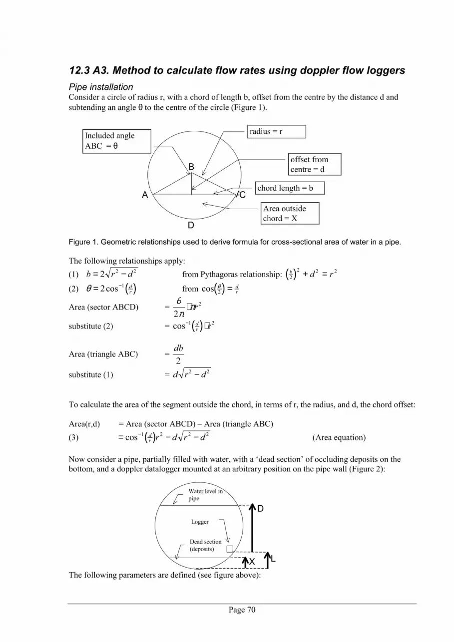
Page 70
12.3 A3. Method to calculate flow rates using doppler flow loggers
Pipe installation Consider a circle of radius r, with a chord of length b, offset from the centre by the distance d and subtending an angle θ to the centre of the circle (Figure 1). Figure 1. Geometric relationships used to derive formula for cross-sectional area of water in a pipe. The following relationships apply: (1) b r d= −2 2 2 from Pythagoras relationship: ( )b d r2
2 2 2+ =
(2) ( )θ = −2 1cos dr from ( )cos θ
2 = dr
Area (sector ABCD) = θπ
π2
2⋅ r
substitute (2) = ( )cos− ⋅1 2dr r
Area (triangle ABC) = db
2
substitute (1) = d r d2 2− To calculate the area of the segment outside the chord, in terms of r, the radius, and d, the chord offset: Area(r,d) = Area (sector ABCD) � Area (triangle ABC) (3) ( )= − −−cos 1 2 2 2d
r r d r d (Area equation) Now consider a pipe, partially filled with water, with a �dead section� of occluding deposits on the bottom, and a doppler datalogger mounted at an arbitrary position on the pipe wall (Figure 2): The following parameters are defined (see figure above):
radius = r
offset from centre = d
chord length = b
Area outside chord = X
Included angle ABC = θ
A
B
AC
D
Water level in pipe
Logger
Dead section (deposits)
D
X L

Page 71
D = Depth reported by logger (this value can be greater than the diameter of the pipe, if the pipe is below the external water level) L = Height of logger above pipe invert X = depth of deposits in pipe bottom If : P = diameter of pipe T = true depth of water in the pipe = min(D+L, P) Then the cross-sectional area of water in the pipe (Aw) is given by: Aw = Area(P/2, T) � Area(P/2,(P/2-X) Where the function Area(r,d) is defined in (3) above. Finally: Water flow (l/sec) = (Aw in cm2) x (water velocity in cm.s-1) / 1000)


