Embed Size (px)
Citation preview

arX
iv:0
810.
2182
v1 [
mat
h.PR
] 1
3 O
ct 2
008 Phase transition for the Ising model on the
Critical Lorentzian triangulation
Maxim Krikun∗†,1 Anatoly Yambartsev‡,2
October 13, 2008
1 Institut Elie Cartan Nancy (IECN), Nancy-Universite, CNRS, INRIA, Boulevard desAiguillettes B.P. 239 F-54506 Vandœuvre-les-Nancy, France.E-mail: [email protected] affiliation: Google Ireland, Dublin, Ireland2 Department of Statistics, Institute of Mathematics and Statistics, University of Sao
Paulo, Rua do Matao 1010, CEP 05508–090, Sao Paulo SP, Brazil.
E-mail: [email protected]
Abstract
Ising model without external field on an infinite Lorentzian tri-angulation sampled from the uniform distribution is considered. Weprove uniqueness of the Gibbs measure in the high temperature regionand coexistence of at least two Gibbs measures at low temperature.The proofs are based on the disagreement percolation method and ona variant of Peierls method. The critical temperature is shown to beconstant a.s.
Keywords: Lorentzian triangulation, Ising model, dynamical triangu-lation, quantum gravityAMS 2000 Subject Classifications: 82B20, 82B26, 60J80
∗Current affiliation: Google Ireland, Dublin, Ireland.†Partially supported by BQR 2007 UMR7502 IAEM 0039.‡Partially supported by the “Rede Matematica Brasil-Franca, CNPq (306092/2007-7)
and CNPR “Edital Universal 2006” (471925/2006-3).
1

1 Introduction
Triangulations, and planar graphs in general, appear in physics in the contextof 2-dimensional quantum gravity as a model for the discretized time-space.Perhaps the best understood it the model of Euclidean Dynamical Triangu-lations, which can be viewed as a way of constructing a random graph bygluing together a large number of equilateral triangles in all possible ways,with only topological conditions imposed on such gluing. Putting a spin sys-tem on such a random graph can be interpreted as a coupling of gravity withmatter, and was an object of persistent interest in physics since the successfulapplication of matrix integral methods to the Ising model on random latticeby Kazakov [8].
More recently, a model of Casual Dynamical Triangulations was intro-duced (see [9] for an overview). The distinguishing feature of this model isits lack of isotropy — the triangulation now has a distinguished time-likedirection, giving it a partial order structure similar to Minkowski space, andimposing some non-topological restrictions on the way elementary trianglesare glued. This last fact destroys the connection between the model and ma-trix integrals, in particular the analysis of the Ising model requires completelydifferent methods (see e.g. [3]).
From a mathematical perspective, we deal here with nothing but a spinsystem on a random graph. Random graphs, arising from the CDT approach,were considered in [11] under the name of Lorentzian models. In the presentpaper we consider the Ising model on such graphs. When defining the modelwe pursue the formal Gibbsian approach [5]; namely, given a realization ofan infinite triangulation, we consider probability measures on the set of spinconfigurations that correspond to a certain formal Hamiltonian.
Our setting is drastically different from e.g. [8] and [3] in that we do notconsider “simultaneous randomness”, when both the triangulations and spinconfigurations are included into one Hamiltonian. Instead we first samplean infinite triangulation from some natural “uniform” measure, and thenrun an Ising model on it, thus the resulting semi-direct product measure is“quenched”.
A modest goal of this paper is to establish a phase transition for the Isingmodel in the above described “quenched” setting (the “annealed” version ofthe problem is surely interesting, but is also more technically challenging, sowe don’t attempt it for the moment). In Section 3 we use a variant of Peierlsmethod to prove non-uniqueness of the Gibbs measure at low temperature.
2

Quite surprisingly, proving the uniqueness at high temperature is not easy– the difficulty consists in presence of vertices of arbitrarily large degree,which does not allow for immediate application of uniqueness criteria suchas e.g. [14]. We resort instead to the method of disagreement percolation [13],and use the idea of “ungluing”, borrowed from the paper [2], to get rid ofvertices of very high degree.
Finally, in Section 5 we show that the critical temperature is in factnon-random and coincides for a.e. random Lorentzian triangulation. Sec-tion 2 below contains the main definitions and summarizes some of the resultsof [11].
We thank E. Pechersky for numerous useful discussions during the prepa-ration of this paper.
2 Definitions and Main Results
Now we define rooted infinite Lorentzian triangulations in a cylinder C =S1 × [0,∞).
Definition 2.1. Consider a connected graph G embedded in a cylinder C. Aface is a connected component of C\G. The face is a triangle if its boundarymeets precisely three edges of the graph. An embedded triangulation T issuch a graph G together with a subset of the triangular faces of G. Letthe support S(T ) ⊂ C be the union of G and the triangular faces in T .Two embedded triangulations T and T ′ are considered equivalent if there is ahomeomorphism of S(T ) and S(T ′) that corresponds T and T ′.
For convenience, we usually abbreviate “equivalence class of embeddedtriangulations” to “triangulation”. This should not cause much confusion.We suppose that the number of the vertices of G is finite or countable.
Definition 2.2. A triangulation T of C is called Lorentzian if the followingconditions hold: each triangular face of T belongs to some strip S1 × [j, j +1], j = 0, 1, . . . , and has all vertices and exactly one edge on the boundary(S1 × {j}) ∪ (S1 × {j + 1}) of the strip S1 × [j, j + 1]; and the number ofedges on S1 × {j} is positive and finite for any j = 0, 1, . . . .
In this paper we will consider only the case when the number of edgeson the first level S1 × {0} equal to 1. This is not restriction, only it givesformulas more clean.
3

Definition 2.3. A triangulation T is called rooted if it has a root. The rootin the triangulation T consists of a triangle t of T , called the root face, withan ordering on its vertices (x, y, z). The vertex x is the root vertex and thedirected edge (x, y) is the root edge. The x and (x, y) belong to S1 × {0}.
Note that this definition also means that the homeomorphism in the def-inition of the equivalence class respects the root vertex and the root edge.For convenience, we usually abbreviate “equivalence class of embedded rootedLorentzian triangulations” to “Lorentzian triangulation” or LT.
In the same way we also can define a Lorentzian triangulation of a cylinderCN = S1 × [0, N ]. Let LTN and LT∞ denote the set of Lorentzian triangula-tions with support CN and C correspondingly.
2.1 Gibbs and Uniform Lorentzian triangulations.
Let LTN be the set of all Lorentzian triangulations with only one (rooted)edge on the root boundary and with N slices. The number of edges on theupper boundary S1 × {N} is not fixed. Introduce a Gibbs measure on the(countable) set LTN :
PN,µ(T ) = Z−1[0,N ] exp(−µF (T )), (2.1)
where F (T ) denotes the number of triangles in a triangulation T and Z[0,N ]
is the partition function:
Z[0,N ] =∑
T∈LTN
exp(−µF (T )).
The measure on the set of infinite triangulations LT∞ is then defined as aweak limit
Pµ := limN→∞
PN,µ .
It was shown in [11] that this limit exists for all µ ≥ µcr := ln 2.
Theorem 1 ([11]). Let kn be the number of vertices at n-th level in a trian-gulation T for each n ≥ 0.
• For µ > ln 2 under the limiting measure Pµ the sequence {kn} is apositive recurrent Markov chain.
4
• For µ = µcr = ln 2 the sequence {kn} is distributed as the branchingprocess ξn with geometric offspring distribution with parameter 1/2,conditioned to non-extinction at infinity.
Below we briefly sketch the proof of the second part of Theorem 1, adeeper investigation of related ideas will appear in [12].
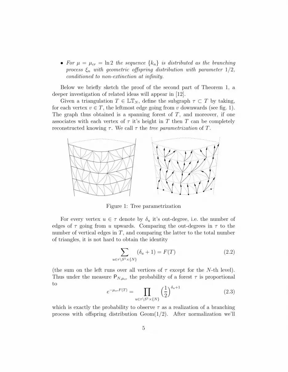
Given a triangulation T ∈ LTN , define the subgraph τ ⊂ T by taking,for each vertex v ∈ T , the leftmost edge going from v downwards (see fig. 1).The graph thus obtained is a spanning forest of T , and moreover, if oneassociates with each vertex of τ it’s height in T then T can be completelyreconstructed knowing τ . We call τ the tree parametrization of T .
Figure 1: Tree parametrization
For every vertex u ∈ τ denote by δu it’s out-degree, i.e. the number ofedges of τ going from u upwards. Comparing the out-degrees in τ to thenumber of vertical edges in T , and comparing the latter to the total numberof triangles, it is not hard to obtain the identity
∑
u∈τ\S1×{N}
(δu + 1) = F (T ) (2.2)
(the sum on the left runs over all vertices of τ except for the N -th level).Thus under the measure PN,µcr
the probability of a forest τ is proportionalto
e−µcrF (T ) =∏
u∈τ\S1×{N}
(1
2
)δu+1
(2.3)
which is exactly the probability to observe τ as a realization of a branchingprocess with offspring distribution Geom(1/2). After normalization we’ll
5

obtain, on the left in (2.3), the probability PN,µ(τ) as defined by (2.1), an onthe right the conditional probability to see τ as a realization of the branchingprocess ξ given ξN > 0. So quite naturally when N → ∞ the distributionof τ converges to the Galton-Watson tree, conditioned to non-extinction atinfinity.
In particular it follows from Theorem 1 that
Pµcr(kn = m) = Pr(ξn = m | ξ∞ > 0) = mPr(ξn = m). (2.4)
Remark 2.1. The last equality in (2.4) means that the measure Pµcron tri-
angulations can be considered as a Q-process defined by Athreya and Ney[1] for a critical Galton-Watson branching process. Such a process is exactlya critical Galton-Watson tree conditioned to survive forever.
We will also note for further use that the offspring generating function ofthe branching process ξ,
ψ(s) =∑
k≥0
(1
2
)k+1
sk =s
2 − s,
and the generating function for ξn (with initial condition ξ0 = 1) is
ψn(s) =n− (n− 1)s
n + 1 − ns.
2.2 Ising model on Uniform Infinite Lorentzian trian-
gulation – quenched case.
Let T be some fixed Lorentzian triangulation, T ∈ LT∞. Let TN be theprojection of T on the cylinder CN . We associate with every vertex v a spinσv ∈ {−1, 1}. Let Σ(T ) and ΣN(T ) denote the set of of all spin configurationson T and TN , respectively. The Ising model on T is defined by a formalHamiltonian
H(σ) =∑
〈v,v′〉∈V
σvσv′ (2.5)
where 〈v, v′〉 means that vertices v, v′ are neighbors, i.e. are connected byan edge in T . Let ∂TN be the set of vertices of T that lie on the circleS1 × {N + 1}. Fix some configuration on the boundary ∂TN and denote it∂σ. The Gibbs distribution with boundary condition ∂σ is defined by the
6

following. Let V (TN) be the set of all vertices in TN , then the energy ofconfiguration σ ∈ ΣN (T ) is
HN(σ|∂σ) =∑
〈v,v′〉: v,v′∈V (TN )
σvσv′ +∑
〈v,v′〉:v∈V (TN ),v′∈∂TN
σvσv′ (2.6)
which defines the probability
P TN,∂σ(σ) =
exp{−βHN(σ|∂σ)}
ZN,∂σ(T )(2.7)
whereZN,∂σ(T ) =
∑
σ∈ΣN (T )
exp{−βHN(σ|∂σ)}.
When N → ∞, for any sequence of boundary conditions ∂σ, a limit (at leastalong some subsequence) of measures P T
N,∂σ exists by compactness. Such alimit is a probability measure on Σ(T ) with a natural σ-algebra, which werefer to as a Gibbs measure.
In general, it is well known that at least one Gibbs measure exists for theIsing model on any locally finite graph and for any value of the parameterβ (see, e.g., [6] page 71). It is also known that the existence of more thanone Gibbs measure is increasing in β, i.e. there exists a critical value βc ∈[0,∞] such that there is a unique Gibbs measure when β > βc, and multipleGibbs measures when β < βc (see [7] for an overview of relations betweenpercolation and Ising model on general graphs).
Thus when considering the Ising model on Lorentzian triangulations it isnatural to ask whether the critical temperature is finite (different from both0 and ∞), and whether it depends on the triangulation. In the following twosections we show that the critical temperature is a.s. bounded both from 0and ∞. In the last section we prove that the critical temperature obeys azero-one law and is therefore a.s. constant.
3 Phase transition at low temperature
In this section we prove the following theorem.
Theorem 2. There exists a β0 such that for all β ∈ (β0,∞) there exist atleast two Gibbs measures for Pµcr
-a.e. T .
7

We remind first the classical Peierls method for the Ising model on Z2.
Let Λ ⊂ Z2 be a large square box centered at the origin, and let P−
Λ be thedistribution for the spins in Λ under the condition that all of the spins outsideof Λ are negative. When the size of the box tends to infinity, P−
Λ convergesto some probability measure P−, which we call Gibbs measure with negativeboundary conditions. The measure P+ is defined similarly taking positiveboundary conditions.
Due to an obvious symmetry between P− and P+ we have
P−(σ0 = +1) = P+(σ0 = −1),
therefore if the Gibbs measure is unique then necessarily P− = P+ and
P−(σ0 = +1) = P−(σ0 = −1) = 1/2. (3.1)
Thus our goal will be to disprove (3.1) for large enough β.Consider some configuration σ such that σ0 = +1 and σi = −1 for all
i /∈ Λ. Define the cluster K+ ⊂ Z2 as the maximal connected subgraph of Z
2,containing the origin, such that σi = +1 for all i ∈ K+. Let γ be the contourin the dual graph (Z2)∗, corresponding to the outer boundary of K+, and letσ′ be the configuration obtained from σ by inverting all the spins inside γ.Note that σ′
0 = −1. Let C be the set of all contours in (Z2)∗ surrounding theorigin, and consider the application
inv : Σ|σ0=+1 → Σ|σ0=−1 × Cσ → (σ′, γ).
(3.2)
Clearly inv is injective: given (σ′, γ) one can easily reconstruct σ by invertingthe spins inside γ. Also the following property holds:
P−Λ (σ) = P−
Λ (σ′) · e−2β|γ|, (3.3)
where |γ| denotes the length of γ. Indeed, for every edge 〈i, j〉 traversedby γ we have σi 6= σj by construction, but after inversion σ′
i = σ′j , so the
contribution of the pair 〈i, j〉 to the Hamiltonian is increased by 2. On theother hand, for all other pairs 〈i, j〉 the contribution to the Hamiltoniandoesn’t change. Informally we can write H(σ) − H(σ′) = 2|γ|, which isequivalent to (3.3).
8

Now taking a sum over all σ : σ0 = +1 in (3.3) we get
P−Λ (σ0 = +1) =
∑
σ:σ0=+1
P−Λ (σ)
≤∑
σ′:σ′
0=−1,γ∈C
P−Λ (σ′) · e−2β|γ|
= P−Λ (σ0 = −1) ·
∑
n≥1
e−2βn#Cn, (3.4)
where Cn is the set of contours γ ∈ C of length exactly n.But #Cn ≤ n3n: indeed, every contour γ ∈ Cn intersects the x-axis
somewhere between 0 and n. Starting from this intersection point there areat most 3n distinct self-avoiding paths of length n in (Z2)∗, only a few ofthem really belonging to Cn. Therefore we have the inequality
P−Λ (σ0 = +1) ≤ P−
Λ (σ0 = −1) ·∑
n≥1
e−2βnn3n, (3.5)
and by taking β large enough the sum in the right-hand side of (3.5) can bemade strictly less than one. Taking the limit Λ → Z
2 we establish
P−(σ0 = +1) < P−(σ0 = −1).
Thus P− 6= P+ and the Gibbs measure for the Ising model in Z2 at inverse
temperature β is not unique.
Figure 2: Peierls’ method on Z2 (left) and on a random Lorentzian triangu-
lation (right). Dashed line represents the inversion contour γ.
Next we will slightly generalize the above classical argument.
9

Lemma 3.1. Let G be an infinite planar graph and G∗ it’s planar dual. Letv0 be a vertex of G and denote by Cn(v0) be the set of contours of length nin G∗, separating v0 from the infinite part of the graph.
If the following sum is finite,
∑
n≥1
#Cn(v0)e−2βn <∞, (3.6)
then the Gibbs measure for the Ising model on G at inverse temperature β isnot unique.
Remark 3.1. Strictly speaking, in the above Lemma we should also requirethe graph G to be one-ended; i.e. for any finite subgraph B ⊂ G the com-plement G\B must contain exactly one infinite connected component. Thereason for this is that if the graph G fails to be one-ended (e.g. a doubly-infinite cylinder) then the outer boundary of the cluster K+ may happen tohave multiple connected components, which slightly complicates the argu-ment. We don’t consider this case in detail since Lorentzian triangulationsare one-ended by construction.
Proof. Assume that (3.6) holds. Then for some large N
∑
n≥N
#Cn(v0)e−2βn < 1.
Also, for every n the set Cn(v0) is finite, so there exists some large R suchthat the ball BR(v0) contains all of the Cn(v0), n = 1 . . . N .
Let now P+ and P− be the Gibbs measures for the Ising model on G,constructed with positive and negative boundary conditions respectively, andlet us compare the events
A+ := (σv = +1 for all v ∈ BR(v0))
andA− := (σv = −1 for all v ∈ BR(v0)).
Proceeding as in the case of Z2 above, we can show that
P−(A+) ≤ P−(A−) ·∑
n≥1
e−2βn#Cn(BR(v0)),
10

where Cn(BR(v0)) now is the set of contours of length n in G∗ that surroundthe whole ball BR(v0). But by construction we have Cn(BR(v0)) = ∅ forn ≤ N and Cn(BR(v0)) ⊂ Cn(v0) for all other n, therefore
∑
n≥1
e−2βn#Cn(BR(v0)) ≤∑
n≥N
e−2βn#Cn(v0) < 1
andP−(A+) < P−(A−).
Since by symmetry P+(A−) = P−(A+), it follows that P− 6= P+.
Lemma 3.2. Let T be a random Lorentzian triangulation, and let v0 be theroot vertex of T . There exists β0 such that for every β > β0
∑
n≥1
#Cn(v0)e−2βn <∞ Pµcr
-a.e., (3.7)
where #Cn(v0) is defined as in Lemma 3.1.
Proof. In order to prove (3.7) it will be sufficient to show that the expectation(with respect to the measure Pµcr
) of the sum is finite
Eµcr
∞∑
n=0
#Cn(0)e−2βn <∞. (3.8)
First of all we choose in any Lorentzian triangulation T a vertical pathγ∞ = γ∞(T ) = (v0, v1, . . . ) starting at the root v0 and such that vi ∈ S1×{i}.Let CR,n(v0) ⊂ Cn(v0) be the set of contours of length n which surround v0
and intersect γ∞ at height R. Note that any such contour does not exit fromthe strip [R− n,R+ n]. Let also SR,n be the number of particles in the treeparametrization of T at height R − n which have nonempty offspring in thegeneration located at height R + n. Since every contour from CR,n, in orderto surround v0, must cross each of the SR,n corresponding subtrees, we have
(SR,n > n) ⇒ (CR,n = ∅).
On the other handCR,n ≤ 2n
since the contours CR,n live on the dual graph T ∗, which has all vertices ofdegree 3, thus there are at most 2n self-avoiding paths with a fixed startingpoint (which is in our case the intersection with γ∞).
11

Therefore we have
Eµcr
∞∑
n=0
#Cn(v0)e−2βn ≤
∞∑
n=0
e−2βn2n
∞∑
R=1
Pµcr(SR,n ≤ n) (3.9)
and for this sum to be finite it’s enough to show that sum over R has poly-nomial order in n. First let us estimate
∞∑
R=1
Pµcr(SR,n ≤ n) ≤ n5 +
∞∑
R≥n5
Pµcr(SR,n ≤ n).
and write for some ǫ ∈ (0, 1/4)
Pµcr(SR,n ≤ n) =
∑
k≤Rǫ
Pµcr(SR,n ≤ n | kR−n = k)Pµcr
(kR−n = k)
+∑
k>Rǫ
Pµcr(SR,n ≤ n | kR−n = k)Pµcr
(kR−n = k).(3.10)
The first sum above satisfies the inequality
∑
k≤Rǫ
Pµcr(kR−n = k) = Pµcr
(kR−n ≤ Rǫ) ≤( Rǫ
R− n
)2
. (3.11)
Indeed, thanks the representation (2.4) the generating function ϕn(s) of kn isrelated to the generating function ψn(s) of the branching process ξn describedabove by the following equation
ϕn(s) = sψ′n(s). (3.12)
Since ψn(s) can be calculated explicitly
ψn(s) =n− (n− 1)s
n + 1 − ns, (3.13)
from (3.12) and (3.13) we obtain
ϕn(s) =s
(1 + n− ns)2, (3.14)
Pµcr(kn = k) =
1
k!
dk
dskϕn(s)
∣∣∣s=0
=knk−1
(n+ 1)k≤
k
n2, (3.15)
12

and ∑
k≤Rǫ
Pµcr(kR−n = k) ≤
∑
k≤Rǫ
k
(R− n)2≤
R2ǫ
(R− n)2,
which proves the estimate (3.11). Since ǫ < 1/4 there exists a constant c1such that ∑
R≥n5
R2ǫ
(R− n)2< c1. (3.16)
The second sum in (3.10) can be estimated by the probability Pµcr(SR,n ≤ n |
kR−n = Rǫ). To do this, let us remind some properties of conditioned or size-biased Galton-Watson trees (see e.g. [10], [4] or [1]). If τ is a Galton-Watsontree of a critical branching process, conditioned to non-extinction at infinity,then conditionally on kR−n the subtrees of τ , originating on the (R − n)-thlevel, are distributed as follows: one subtree, chosen uniformly at random, hasthe same distribution as τ (i.e. is infinite), while the remaining subtrees areregular Galton-Watson trees corresponding to the original branching process(and are finite a.s.).
The probability for a particle of the branching process ξ to survive up totime 2n equals 1/(2n+ 1), thus conditionally on kR−n, SR,n is stochasticallyminorated by the binomial distribution with parameters (kR−n,
12n+1
). UsingHoeffding’s inequality for binomial distribution we obtain
Pµcr(SR,n ≤ n | kR−n = Rǫ) < exp
(−2
(Rǫ/(2n+ 1) − n)2
Rǫ
)(3.17)
and the sum over R > n5 is bounded by some absolute constant c2
∑
R>n5
exp(−2
(Rǫ/(2n+ 1) − n)2
Rǫ
)≤ e2
∑
R>n5
exp(−
2Rǫ
(2n + 1)2
)< c2. (3.18)
Thus we have proved that
Eµcr
∞∑
n=0
Cn(0)e−2βn ≤∞∑
n=0
e−2βn2n(n5 + c1 + c2) (3.19)
and so for all β > ln 22
the sum (3.7) is finite.Proof of Theorem 2. Theorem 2 follows immediately from Lemmas 3.1and 3.2.
13

4 Uniqueness for high temperature
In this section we prove the following theorem
Theorem 3. There exists a small enough βh such that for every β ∈ [0, βh)for Pµcr
-a.e. Lorentzian triangulation T the Gibbs measure for the Ising modelon T is unique.
The proof goes as follows. First, for a fixed triangulation T we use dis-agreement percolation to reduce the problem of uniqueness of a Gibbs mea-sure to the problem of existence of an infinite open cluster under some specificsite-percolation model on T . Then we consider the joint distribution of a tri-angulation with this percolation model on it (i.e. with randomly open/closedvertices), where the triangulation T is distributed according to Pµcr
, and con-ditionally on T the state of each vertex in T is chosen independently (butwith vertex-dependent probabilities). We show that the probability for sucha random triangulation to contain an infinite open cluster is 0, therefore thisprobability is 0 for Pµcr
-a.e. triangulation as well, and the theorem follows.
4.1 Disagreement percolation
The following result of Van den Berg and Maes [13] provides a sufficientcondition for the uniqueness of the Gibbs measure, expressed in terms ofsome percolation-type problem.
Theorem 4. Let G be a countably infinite locally finite graph with the vertexset V , and let S be a finite spin space. Let Y be a specification of a Markovfield on G, i.e. for every finite A ⊂ V , YA(·, η) is the conditional distribu-tion of the spins on A, given that the spins outside of A coincide with theconfiguration η ∈ SV .
Define for every v ∈ V
pv := maxη,η′∈SV
ρvar(Y{v}(·, η), Y{v}(·, η′)),
where ρvar denotes the distance in variation. Let P p,G be the product mea-sure under which each vertex v is open with probability pv and closed withprobability 1 − pv.
If under site-percolation on G, one has
P p,G{there is an infinite open path} = 0,
then the specification Y admits at most one Gibbs measure.
14

In the case of the Ising model, the only spins that affect the distributionof the spin at a given vertex v are those at vertices u connected to v by anedge (denoted u ∼ v). Let dv be the degree of v and let Sv =
∑u∼v σu. The
conditional distribution of σv, given the values of spins σu for all u ∼ v, onlydepends on Sv and is given by
P T{σv = +1|Sv} =e−βSv
e−βSv + eβSv, P T{σv = −1|Sv} =
eβSv
e−βSv + eβSv.
The distance in variation between two such conditional distributions is max-imized by taking two extreme values of Sv, namely Sv = dv and Sv = −dv,corresponding to all-plus and all-minus boundary conditions. Therefore wehave
pv =1
2
(∣∣∣e−βdv
e−βdv + eβdv−
eβdv
e−βdv + eβdv
∣∣∣
+∣∣∣
e−βdv
e−βdv + eβdv−
eβdv
e−βdv + eβdv
∣∣∣)
= tanh(βdv)
and we need to prove the following
Lemma 4.1. Let T be an infinite random Lorentzian triangulation sampledfrom the measure Pµcr
, and let each vertex v ∈ T be open with probabilitypv = tanh(βdv) and closed otherwise. Then for small enough β the probabilitythat there is an infinite open path in T is zero.
4.2 Elementary approach to non-percolation
Imagine for a moment that the graph G that we deal with in Lemma 4.1has uniformly bounded degrees. If with positive probability there exists aninfinite open percolation cluster, then with positive probability this clusterwill also be connected to the origin. Consider the event
An =
{there exists a self-avoiding open path of length n
starting at the origin.
}
The number of paths of length n, starting at the origin, is at most Dn,where D is the maximal degree of a vertex in our graph. Obviously the sameestimate is valid for the number of self-avoiding paths. The probability for avertex to be open is bounded by tanh(βD) ≤ βD, therefore we can estimate
P p,G(An) ≤ Dn tanh(βD)n ≤ βnD2n.
15

Taking β < 1/D2, we get P p,G(An) → 0 as n → ∞, and therefore theprobability that the origin belongs to an infinite open cluster is zero.
Unfortunately, the above argument can’t be applied directly in the con-text of Lemma 4.1: in an infinite random Lorentzian triangulation with prob-ability one one will encounter regions consisting of vertices of arbitrarily largedegrees, and these regions can be arbitrarily large as well. On the other hand,we know that in a Lorentzian triangulation the degree of a typical vertex isnot too large (in some sense, which we’re not going to make precise in thispaper, it can be approximated by a sum of two independent geometric dis-tributions plus a constant), therefore one can hope to show that the verticesof very large degree are so rare that they don’t mess up the picture.
Before proceeding further, let us remark that in the above argument onecan consider, instead of the set of all the self-avoiding paths, only the pathsthat are both self-avoiding and locally geodesic. We say that a path γ ina graph G is locally geodesic if whenever two vertices, belonging to γ, areconnected by and edge in G, this edge also belongs to γ (in other words, alocally geodesic path avoids making unnecessary detours). Clearly, if undersite percolation on G there exists an infinite open self-avoiding path startingat v0, there exists also an infinite self-avoiding locally geodesic path. It isalso easy to see that if γ is a locally geodesic path, then every vertex v ∈ γhas at most two neighbors belonging to γ. We will use this observation inthe next section.
4.3 Generalization to random triangulations
Fix an infinite Lorentzian triangulation T and let γ be a finite self-avoiding,locally geodesic path in T , starting at the root vertex (which we denote byv0). Let Γ ⊂ T be a 1-neighborhood of γ, i.e. a sub-triangulation consisting ofthe path γ together with all triangles, adjacent to γ. Such a sub-triangulationenjoys the rigidity property: if Γ can be embedded into some Lorentzian tri-angulation, then this embedding is unique1. We define the event “T containsΓ” (denoted Γ ⊂ T ) to be the subset of triangulations in LT∞ for which suchan embedding exists.
Lemma 4.2. Let Γ be a 1-neighborhood of a locally geodesic path γ, let γhave length n and let the vertices of γ have degrees d0, d1, . . . , dn.
1 we require that the embedding maps v0 to the root vertex of T , and sends horizon-tal/vertical edges of Γ to edges of the same type in T
16

The probability that a random Lorentzian triangulation T contains Γ isbounded by
Pµcr{Γ ⊂ T} ≤ Cn
n∏
i=0
1
d9i
for some absolute constant C.
We can use this lemma to obtain estimates on percolation probability asfollows. Given the degrees d0, . . . , dn one can completely specify Γ using thefollowing collection of numbers
• for each vertex we need to specify how it’s degree dj is split into d(up)j
and d(dn)j , i.e. edges going up and down from the vertex — this gives
one integer parameter in the range [1, dj];
• also we need to specify the edge along which the path γ entered thevertex and the edge along which it left; this adds two more parameters.
The total number of meaningful combinations for the above parametersclearly does not exceed
∏d3
j . Now, if T is a Pµcr-distributed random tri-
angulation with site-percolation on it, by Lemma 4.2 the probability for Tto contain an open path from the origin with vertex degrees d0, . . . , dn isbounded by
∏
j
C
d9j
×∏
j
tanh(βdj) ×∏
j
d3j ≤ (βC)n
∏ 1
d5j
.
Summing over all possible values of d0, . . . , dn we obtain the estimate
∑
d0,...,dn
(βC)n∏ 1
d5j
≤(βC
∑
d≥4
1
d5
)n
for the probability to have an open path of length n in a random triangula-tion. For β sufficiently small, the last expression tends to 0 as n → ∞, andthe probability to have an infinite open path from the origin is zero.
Note that here we are estimating the annealed probability (semi-directproduct Pµcr
×P p,T ) of the existence of open path. Clearly, if this annealedprobability is zero, then also for Pµcr
-a.e. triangulation T the P p,T -probabilityof an infinite open path is zero as well.
Therefore it remains to prove Lemma 4.2.
17

4.4 Elementary perturbations
Consider a finite Lorentzian triangulation T ∈ LTN containing an internalvertex v of very high degree, say dv ≥ 100. Let d
(up)v and d
(dn)v be the degree
contributed to dv by edges going upwards and downwards from v, so thatdv = d
(up)v +d
(dn)v +2. Let O(v) be a 1-neighborhood of v, i.e. all the triangles
adjacent to v, and let T ′ be the complement to O(v) in T .Let us estimate PN,µ(T |T
′), i.e. the probability to see T as a realizationof a random Lorentzian triangulation, conditionally on the event that thistriangulation contains T ′. For this purpose consider a modification of the1-neighborhood of v, which consists in adding a pair of triangles as shown onfig. 3. There are d
(up)v × d
(dn)v to distinct ways to make such a modification,
Figure 3: Inserting a pair of triangles at a high-degree vertex v. The positionto insert new triangles is determined by the choice of two neighboring verticeson the layers below and above v.
and every time the Hamiltonian of the Gibbs measure (2.1) is increased by2µ (since there are 2 triangles added)
Therefore we can estimate
PN,µ(T | T ′) ≤e2µ
d(up)v d
(dn)v
≤e2µ
(dv − 2)/2.
A better estimate can be obtained by applying k elementary perturbationsat v simultaneously. Such a set of perturbations is specified by a sequenceof pairs {(u
(up)i , u
(dn)i )}k
i=1 of vertices lying on the layers above and below v(fig. 4).
In order to assure that all the perturbations can be applied unambigu-ously, we require that the vertices u
(up)1 , . . . u
(up)k to be ordered from left to
right, as well as u(dn)1 , . . . u
(dn)k . We may however allow some vertices to coin-
cide – otherwise it would be impossible to apply n perturbations at once ina vertex whose up-degree or down-degree are not large enough.
18

Figure 4: Multiple insertions at the same vertex. Note that one of the edgesis used twice for insertions, and the corresponding vertex has two dots.
If dv is large, one of d(up)v or d
(dn)v is at least (dv − 2)/2, and therefore the
number of distinct ways to choose, say, k = 10 modifications is at least(
(dv − 2)/2
10
)= C10d
10v +O(d9
v).
Now consider a path γ ⊂ Γ with vertices of degrees d0, . . . , dn. Let WΓ
be the set of possible modifications we can make to Γ, by inserting exactly10 pairs of triangles at vertices of high degree (say, di ≥ 100), and leaving all
other vertices intact. Then for some constant C10
#WΓ ≥∏
C10d10j .
Let LTΓ,N ⊂ LTN be the set of Lorentzian triangulations that contain Γ.Clearly, each modification w ∈ WΓ can be applied to every T ∈ LTΓ,N ,producing a modified triangulation which we denote by w(T ). Consider theapplication of modifications w to a triangulation T as a mapping
app : LTΓ,N ×WΓ → LTN
(T, w) → w(T ).(4.1)
Since any modification to T ∈ LTΓ,N adds at most 20n new triangles, wehave, for all (T, w) ∈ LTΓ ×WΓ
PN,µ(w(T )) ≥ e−20nµPN,µ(T ).
Taking a sum over all (T, w) we get
∑
(T,w)∈LTΓ,N×WΓ
PN,µ(w(T )) ≥ e−20nµ#WΓ
∑
T∈LTΓ,N
PN,µ(T ) (4.2)
= e−20nµ#WΓ PN,µ(Γ).
19

4.5 Overcounting via random reconstruction
In order to get an estimate on PN,µ(Γ) from (4.2), it would be helpful if theapplication (4.1) was an injection. But this is not easy to prove (if at alltrue!), so instead we will estimate the overcounting
overΓ(T ′) := #{(T, w) ∈ LTΓ,N ×WΓ |w(T ) = T ′}.
Lemma 4.3. Given a path γ with 1-neighborhood Γ, with vertex degreesd0, . . . , dn, we have for any T ′ ∈ LTN
overΓ(T ′) ≤∏
12(dj + 10). (4.3)
Proof. First note that each elementary perturbation (i.e. insertion of twoadjacent triangles) can be undone by collapsing the newly inserted horizontaledge. Therefore in order to reconstruct the pair (T, w), knowing T ′ = w(T ),it will be sufficient to identify the edges of T ′ that were added by w.
It’s not clear whether we can perform such a reconstruction determinis-tically, but we certainly can achieve it with some probability with the help ofthe following randomized algorithm:
• the algorithm starts from the root vertex and at each step moves to anadjacent vertex, chosen uniformly at random;
• it also modifies the triangulation along his way as following
• each time arriving to a new vertex it should decide whether to contracta sequence of 10 horizontal edges (at least one of these edges must beadjacent to the current location), or do nothing. This gives 12 = 11+1possibilities, among which one is chosen uniformly at random.
• after n steps, the path traversed by the algorithm is declared to be the(conjectured) path γ, and if it really is, and if the resulting triangu-lation coincides with the original triangulation t, the reconstruction isconsidered successful.
Most of the time this algorithm will fail, but with some probability it mayactually reconstruct both T and w. Let us now estimate this probability.
First note that the degree of v0 in T ′ can be larger than the degree ofv0 in T because of the modifications made to the second vertex of γ, but inany case it will not exceed d0 + 10, since each elementary modification in v1
20

increases the degree of v0 at most by 1. Therefore, the algorithm will guessthe correct direction from v0 with probability at least 1/(d0 + 10).
Assuming the direction it took on the first step was correct, there isexactly 1 right choice out of 12 on the next step (collapse some 10 nearbyhorizontal edges, which can be chosen in 11 different ways, or do nothing),so the probability not to fail is 1/12.
Assuming again that the modifications to the second vertex v1 were un-done correctly, there is at least one edge that will lead to the next vertex v2.Since the path γ is locally geodesic, at most two neighbors of v1 belong toγ, namely these are v0 and v2. Modifications at v2 add at most 10 to thedegree of v1, so with probability at least 1/(d1 + 10) the algorithm will takethe correct direction again.
Proceeding this way, we see that the probability to win is at leastn∏
j=0
1
12(dj + 10). (4.4)
Now for every T ′ and for every (T, w) ∈ LTΓ,N ×WΓ such that w(T ) =T ′ the probability to correctly reconstruct (T, w) from T ′ is at least (4.4),therefore
overΓ(T ′) ≤∏
12(dj + 10).
This finishes the proof of Lemma 4.3Finally, combining the inequalities (4.2) and (4.3) we get
e−20nµ#WΓ PN,µ(Γ) ≤∑
(T,w)∈LTΓ,N×WΓ
PN,µ(w(T ))
≤∑
T ′∈LTN
overΓ(T ′) PN,µ(T ′)
≤n∏
j=0
12(dj + 10)∑
T ′∈LT
PN,µ(T′)
≤n∏
j=0
12(dj + 10),
and
PN,µ(Γ) ≤
e20nµn∏
j=0
12(dj + 10)
n∏j=0
C10d10j
≤n∏
j=0
e20µC
d9j
.
21

Since the last estimate is uniform in N , it holds also for the limiting mea-sure Pµ, and setting µ = µcr we obtain the statement of Lemma 4.2. Thisalso finishes the proof of Theorem 3.
5 Critical temperature is constant a.s.
Consider the critical temperature βc(G) of the Ising model on a graph G asa function of G. In the above two sections we have shown that when T is aPµcr
-random Lorentzian triangulation, we have βc(T ) ∈ [βh, β0] a.s. In thissection we show that in fact
Theorem 5. βc(T ) is constant Pµcr-a.s.
The proof relies on two lemmas.
Lemma 5.1. Let G, G′ be two locally finite infinite graphs that differ onlyby a finite subgraph, i.e. there exist finite subgraphs H ⊂ G, H ′ ⊂ G′ suchthat G\H is isomorphic to G′\H ′. Then βc(G) = βc(G
′).
Proof. This statement is widely known and follows from Theorem 7.33 in [5].More exactly, consider the Ising model on G at some fixed inverse tem-
perature β ∈ (0,∞). Let Y be the corresponding specification (collectionof conditional distributions) and denote by G(Y ) the set of Gibbs measures,satisfying this specification. It is an easy fact that G(Y ) is a convex set inthe linear space of finite measures on the set of configurations.
Any specification Y on G can be naturally restricted to a specification Yon G\H . Namely, for each finite A ⊂ G\H and each η ∈ {−1, 1}G\H put
YA(·, η) = P{σi = (·)i ∀i ∈ A; σi = ηi ∀i ∈ (G\H)\A}.
=∑
eη∈{−1,+1}H
YA∪H((·)∪η | η) (5.1)
(the last sum runs over all spin configurations in H). Informally, the re-
stricted specification Y can be interpreted as an Ising model on G, but withthe spins in H being hidden from the observer.
Let now Y ′ be the specification for the Ising model on G′, and let Y ′ be ananalogous restriction of Y ′ to G′\H ′. Since G\H and G′\H ′ are isomorphic,
the specifications Y and Y ′ are defined over the same graph, and it follows
22

from (5.1) that they are equivalent in that there exists a constant c > 1 suchthat
1
c<YA(· | η)
Y ′A(· | η)
< c
for all possible values of A, η and (·). Theorem 7.33 in [6] then implies that
G(Y ) is affinely isomorphic to G(Y ′). In particular G(Y ) consists of a single
element – a unique Gibbs measure – if and only if G(Y ′) does.
Since any Gibbs measure on spin configurations in G\H , satisfying Y ,can be uniquely extended to a Gibbs measure on G, satisfying Y , and thesame holds for G′, H ′, Y ′, the lemma follows.
Lemma 5.2. A Galton-Watson tree for a critical branching process, condi-tioned to non-extinction at infinity, can be described as following
• it contains a single infinite path (a spine), {v0, v1, . . .}, starting at theroot vertex;
• at each vertex vi of the spine a pair of finite trees (Li, Ri) is attached,one of each side of the spine;
• and the pairs (Li, Ri) are independent and identically distributed.
Remark 5.1. In fact, the law of (Li, Ri) can be explicitly expressed in termsof the original branching process, but for our purposes it’s enough to knowthat the trees are i.i.d.
Proof. See e.g. [10] or [4].
Proof of Theorem 5. Consider now the tree parametrization τ of a Pµcr-
distributed infinite Lorentzian triangulation T . By Lemma 5.2, τ is encodedby a sequence of pairs of finite trees (Li, Ri)i∈Z. Clearly, this is an exchange-able sequence. Let σij be a permutation of the i-th and j-th pairs; thenσijτ is a tree-parametrization of some other infinite Lorentzian triangula-tion σijT , which only differs from T by a finite subgraph. By Lemma 5.1βc(T ) = βc(σijT ), and Hewitt-Savage zero-one law applies to βc, consideredas a function of the sequence (Li, Ri)i∈Z. Thus βc(T ) is constant a.s.
23

References
[1] Krishna B. Athreya and Peter E. Ney, Branching processes, Springer-Verlag, New York, 1972, Die Grundlehren der mathematischen Wis-senschaften, Band 196. MR MR0373040 (51 #9242)
[2] L. A. Bassalygo and R. L. Dobrushin, Uniqueness of a Gibbs field with arandom potential—an elementary approach, Teor. Veroyatnost. i Prime-nen. 31 (1986), no. 4, 651–670. MR MR881577 (88i:60160)
[3] D. Benedetti and R. Loll, Quantum gravity and matter: Counting graphson causal dynamical triangulations, General Relativity and Gravitation39 (2007), 863–898.
[4] Jochen Geiger, Elementary new proofs of classical limit theorems forGalton-Watson processes, J. Appl. Probab. 36 (1999), no. 2, 301–309.MR MR1724856 (2001k:60119)
[5] Hans-Otto Georgii, Gibbs measures and phase transitions, de GruyterStudies in Mathematics, vol. 9, Walter de Gruyter & Co., Berlin, 1988.MR MR956646 (89k:82010)
[6] Hans-Otto Georgii, Olle Haggstrom, and Christian Maes, The randomgeometry of equilibrium phases, Phase transitions and critical phenom-ena, Vol. 18, Phase Transit. Crit. Phenom., vol. 18, Academic Press,San Diego, CA, 2001, pp. 1–142. MR MR2014387 (2004h:82022)
[7] Olle Haggstrom, Markov random fields and percolation on generalgraphs, Adv. in Appl. Probab. 32 (2000), no. 1, 39–66. MR MR1765172(2001g:60246)
[8] V.A. Kazakov, Ising model on a dynamical planar random lattice: Exactsolution, Phys. Lett. A 119 (1986), 140–144.
[9] R. Loll, J. Ambjorn, and J. Jurkiewicz, The universe from scratch, Con-temporary Physics 47 (2006), 103–117.
[10] Russell Lyons, Robin Pemantle, and Yuval Peres, Conceptual proofs ofL logL criteria for mean behavior of branching processes, Ann. Probab.23 (1995), no. 3, 1125–1138. MR MR1349164 (96m:60194)
24
[11] V. Malyshev, A. Yambartsev, and A. Zamyatin, Two-dimensionalLorentzian models, Mosc. Math. J. 1 (2001), no. 3, 439–456, 472. MRMR1877603 (2002j:82055)
[12] V. Sisko, A. Yambartsev, and A. Zamyatin, Uniform infinite lorentziantriangulation and critical branching process, in preparation.
[13] J. van den Berg and C. Maes, Disagreement percolation in the study ofMarkov fields, Ann. Probab. 22 (1994), no. 2, 749–763. MR MR1288130(95h:60154)
[14] Dror Weitz, Combinatorial criteria for uniqueness of Gibbs mea-sures, Random Structures Algorithms 27 (2005), no. 4, 445–475. MRMR2178257 (2006k:82036)
25


