Embed Size (px)
Citation preview

Matrix Elements of Lorentzian Hamiltonian Constraint in LQG
Emanuele Alesci,1, ∗ Klaus Liegener,2, † and Antonia Zipfel2, ‡
1Instytut Fizyki Teoretycznej, Uniwersytet Warszawski,ul. Hoża 69, 00-681 Warszawa, Poland, EU
2Universität Erlangen, Institut für Theoretische Physik III, Lehrstuhl für QuantengravitationStaudtstrasse 7, D-91058 Erlangen, EU
(Dated: July 22, 2013)
AbstractThe Hamiltonian constraint is the key element of the canonical formulation of LQG coding its dynamics. In
Ashtekar-Barbero variables it naturally splits into the so called Euclidean and Lorentzian parts. However, due tothe high complexity of this operator, only the matrix elements of the Euclidean part have been considered so far.Here we evaluate the action of the full constraint, including the Lorentzian part. The computation requires anheavy use of SU(2) recoupling theory and several tricky identities among n-j symbols are used to find the finalresult: these identities, together with the graphical calculus used to derive them, also simplify the Euclidean
constraint and are of general interest in LQG computations.
∗ [email protected]† [email protected]‡ [email protected]
arX
iv:1
306.
0861
v2 [
gr-q
c] 1
8 Ju
l 201
3

2
I. INTRODUCTION
In the Hamiltonian formulation General Relativity (GR) is completely governed by the Diffeomorphism
and Hamiltonian constraints. For many years the complicated structure of these constraints prevented a
quantization of the theory, until Ashtekar [1] suggested to replace the "old" metric variables by connections
and tetrads. Indeed in this variables GR resembles other gauge theories, like Yang-Mills theory, whereupon
one encounters an SU(2)-Gauss constraint in addition to Diffeomorphism and Hamiltonian constraints.
This formulation was further improved by Barbero [2] and serves today as the classical starting point of
Loop Quantum Gravity (LQG) [3–5].
LQG follows the Dirac quantization program [6] for constrained systems, i.e. one introduces a prelim-
inary kinematical Hilbert space on which the constraints can be represented by operators and then seeks
for the kernel of these operators defining the physical Hilbert space. The Gauss constraint is solved by
introducing a so called "spin network" basis [7], naturally leading to a combinatorial discrete structure of
space-time similar to the one proposed by Penrose [8], while the Diffeomorphisms constraint is solved by
considering equivalence class of spin networks under diffeomorphisms denoted "s-knots" [9].
A major obstacle for completing the canonical quantization program in LQG is the implementation of
the Hamiltonian constraint S. The difficulties are mainly caused by the non-polynomial structure of S
and the weight factor 1/√
det(q) determined by the intrinsic metric q := qab on the initial hypersurface
Σ. In fact, Ashtekar [1] was motivated by the observation that the Hamiltonian constraint can be casted
into a polynomial form when the metric variables are replaced by triads and complex connections. Even
though this simplifies the constraint one has to deal instead with difficult reality conditions. This reality
structure is of course trivial when the theory is formulated in real connection variables as suggested by
Barbero [2]. Unfortunately, the constraint remains to be non-polynomial in these variables. It was then
proposed to absorb the weight 1/√
det(q) in the Lapse-function. But it turned out [10] that this density
weight is crucial in order to obtain a finite, background independent operator.
After many efforts [11], Thiemann [12] discovered that both problems, the non-polynomiality and the
appearance of the weight factor, can be solved by expressing the inverse triads through the Poisson bracket
of volume and connections ("Thiemann trick"). This trick made it possible to construct a finite, anomaly-
free operator that corresponds to the non-rescaled Hamiltonian constraint [4, 12, 13] and acts by changing
the underlying graph of the spin networks. The formal solution [13] to this constraint are superpositions of
s-knot states with "dressed nodes", that are nodes with a spider-web like structure. Criticism appeared [14]
mostly concerning the "ultralocal" character of the construction and regularization ambiguities. However
until now, this is the only known scheme able to realize an anomaly free quantization of the Dirac algebra
at least on shell.
This construction is at the heart of many other approaches within canonical LQG, as the master
constraint program [15], Algebraic Quantum Gravity (AQG) [16], most recent models with matter [17–19]
and symmetry reduced models like Loop Quantum Cosmology [20, 21]. Also the covariant approach (spin

3
foam models) [22] is motivated by the idea of realizing the "time-evolution" generated by a graph-changing
Hamiltonian [23]. In fact, it is hoped that the spin-foam model might provide a physical scalar product
for canonical LQG (see e.g. [24]). The attempt to match both approaches (not only heuristically) has
led to new regularization schemes for the Hamiltonian constraint [25, 26] and also to the discovery of new
physical states in the canonical model [27].
Despite it’s central role for LQG the action of S has been analyzed explicitly in only very few examples
[27–29] and these are confined to the Euclidean part of the constraint only. This is mainly due to two
reasons: first the presence of the volume operator [30, 31] and second the non trivial recoupling of SU(2)
irreducible representations. The volume operator in LQG has been studied intensively in [32–34]. Yet,
the matrix elements are getting very complicated the more edges are involved so that one has to apply
numerical methods [35, 36] to evaluate it. The second difficulty appears due to the regularization of the
connections by holonomies. The corresponding operators act by multiplication which produces several
Clebsh-Gordan decompositions and modifications to the intertwiners between SU(2) representations at
the nodes.
In this paper we explicitly compute the matrix elements of the full Lorentzian constraint in the Thie-
mann prescription for trivalent nodes. The final result still depends on the matrix elements of the volume
which are unknown in closed form, but in principle computable. In the course of the evaluation several
recoupling identities will be proven, which greatly simplify the final result and are expected to be useful in
all the computations involving curvature loops or the "Thiemann trick". The resulting compact formula
presented here opens the possibility to test the implementation of the constraint by simulations, analyze
the behavior of S in a large j-limit or further develop the methods of [27].
The article is organized as follows: In Section II Thiemann’s construction for the Euclidean and
Lorentzian term is briefly reviewed and in Section III the main recoupling identities are introduced that
will then be applied in Section IV to the Euclidean constraint leading to a new and very compact expres-
sion for it. Finally in Section V, we present the matrix elements of the Lorentzian part. Section VI is left
for concluding remarks and an Appendix with further details on n-j symbols and the Volume operator is
included to make the manuscript self-contained.
II. HAMILTONIAN CONSTRAINT
A. Classical constraint
Let eia be a triad on a smooth, spatial hypersurface Σ defining the intrinsic metric qab = δijeiaejb.
Here, a, b = 1, 2, 3 are tensorial and i, j = 1, 2, 3 are su(2)-indices. In the following, Γia denotes the spin-
connection associated to eia and Kab the extrinsic curvature. Given Kia := sgn(det(ejc))ebiKab, it can be
shown that the densitized inverse triad Eai :=√
det(q)eai and Aia := Γia+γKi
a form a canonical conjugated

4
pair,
{Aia(x), Ebj (y)} = κδijδbaδ
(3)(x, y) , (1)
where γ is a real non-zero parameter and κ = 8πGc3γ. If Fab denotes the curvature of A and s the signature
of the space-time metric then the classical Hamiltonian constraint is of the form
S =1√
det(q)Tr{(Fab − (γ2 − s)[Ka,Kb])[E
a, Eb]} . (2)
According to [12], the square root in (2) can be absorbed by using Poisson brackets of the connection
A with the Volume,
V := V (Σ) =
ˆΣ
dx3√
det(q) , (3)
and the integrated curvature,
K :=
ˆΣ
dx3EajKja . (4)
More explicitly, inserting
[Ea, Eb]i√det(q)
= −2
κεabc{Aic(x), V } and Ki
a =1
κ{Aia(x),K} (5)
in (2) yields
H =2
κεabc Tr(Fab{Ac, V }) (6)
and
T := S −H = (s− γ2)4
κ3εabc Tr({Aa,K}{Ab,K}{Ac, V }) , (7)
where S was split into an Euclidean part H and remaining constraint T , which vanishes for γ2 = 1 and
s = 1. The second part (7) can be further modified by expressing K through the ’time’ derivative of the
volume:
K = − 1
κγ{V,ˆ
Σdx3H} . (8)
Thus S is completely determined by the connection A, the curvature F and the volume V all of which
have well-defined operator analogous in LQG.
B. Quantization
Prior to quantization the local expressions (6) and (7) must be smeared and regularized. That is to say
the connection and curvature of the integrated constraint S[N ] :=´
ΣN(x)S(x) are replaced by holonomies

5
aki
n si
sjsk aij
ajk
Figure 2.1. An elementary tetrahedron ∆ ∈ T
constructed by adapting it to a graph Γ.
along edges and loops respectively. Of course the properties of the operator depend highly on the chosen
regularization and up to now there are several different models on the market (see e.g. [3, 12, 26]). Here,
we follow the original proposal [12] because it is comparatively easy and leads to anomaly free and finite
operators.
Since the Euclidean constraint H[N ] depends linearly on the volume and the volume operator is acting
locally on the nodes it suffices to construct a regularization in the neighborhood of a node n in a given
graph Γ and then extend it to all of Σ. Let sI be a segment of an edge eI incident at n and αIJ the loop
generated by sI and sJ . I.e. αIJ = sI ◦ aIJ ◦ s−1J where aIJ is a semi-analytic arc which only intersects
with Γ in the endpoints of sI and sJ (see Fig. 2.1). In this way, any three (non-planar) edges eI , eJ and
eK incident at n constitute an elementary tetrahedron ∆IJK . Starting with ∆IJK one can now construct
seven additional tetrahedra (see [12] for details), such that the eight tetrahedra including ∆IJK cover
a neighborhood of n. Afterwards this is extended to a full triangulation1 T(I, J,K) of Σ and H[N ] is
decomposed into∑
∆∈TH∆[N ].
On the elementary tetrahedron ∆IJK the connection A and the curvature F are regularized as usual by
smearing along sK and αIJ respectively so that the regularized constraint is defined by
H∆IJK[N ] : =
∑i,j,k∈{I,J,K}
2
3κN(n) εijk Tr
[hαijhsk
{h−1sk, V}]
, (9)
where hs is the holonomy alongside s and N(n) is the value of the lapse function N(x) at n. In the article
[29] it was proposed to generalize this by considering holonomies in an arbitrary irrep m that yields
Hm∆IJK
[N ] :=∑
i,j,k∈{I,J,K}
N(n)
N2mκ
εijk Tr[h(m)αij h
(m)sk
{h
(m)
s−1k
, V}]
, (10)
with the normalization factor N2m = (2m+ 1)m(m+ 1). At this point, the quantization of (10) is straight
forward. Its action on a cylindrical function Ts on a spin net s with underlying graph Γ is
H[N ]Ts =i
N2m κ l
2p
∑n∈Γ
8N(n)
E(n)
∑n(∆)=n
εijk Tr
(h(m)αij h
(m)sk
[h(m)
s−1k
, V ]
)Ts . (11)
1 Note, for each triple of edges adjacent to a node one constructs an independent triangulation.

6
H−−−−−→
m
T−−−−→
m
m
Figure 2.2. The Euclidean constraint H creates a new link (red) joining two edges at the samevertex due to the regularization of the curvature. Note, the new nodes are coplanar whereby two ofthe adjacent edges are even colinear. On the right hand side the principal action of T is visualized:The red link is created by the first extrinsic curvature while the blue one is created by the secondcurvature operator that is regularized along a tetrahedron lying inside of the first one.
The first sum is running over all nodes of Γ and the second over all elementary tetrahedra. lp is the Planck
length. Because every vertex is surrounded by 8 tetrahedra the smearing of H in the neighborhood of
n yields eight times the same factor. Apart from that, at an m-valent vertex n there are E(n) :=(m3
)elementary tetrahedra each of which determines an adapted triangulation. Therefore we need to divide
by E(n) to avoid over counting.
A huge advantage of the operator defined above is that it is anomaly free, i.e. that the commutator of
two constraints H is vanishing up to diffeomorphisms. This is mainly due to the behavior of the volume
which is vanishing on coplanar nodes2. But, in fact, H only generates such nodes (see Fig. 2.2) so that a
second Hamiltonian acts again only on the ’old’ ones.
The remaining part of the constraint T [N ] can be quantized similarly. However, the regularization is a
bit more involved because the extrinsic curvature must be regularized separately. In principle T adds two
new links each of which is created by one operator K := il2p γ
[V , H[1]]. To insure that the full constraint
is still anomaly free only coplanar nodes should be generated. That means, it must never happen that
the two new links have a common intersection. Because H is acting locally the second extrinsic curvature
should be therefore regulated along tetrahedra lying inside of the first ones (see Fig. 2.2). The holonomies
in T can be regulated as above such that finally
T [N ]Ts =2i(s− γ2)
N2m κ l
6p
∑n∈Γ(0)
8N(n)
E(n)
∑n(∆)=n
εijk Tr
(h(m)si [h
(m)
s−1i
, K]h(m)sj [h
(m)
s−1j
, K]h(m)sk
[h(m)
s−1k
, V ]
)Ts . (12)
In (11) and (12) the triangulation T serves as a regulator. This regularization dependence can be removed
by in a suitable operator topology 3.
III. COMPUTATIONAL TOOLS
In this section the tools for computing the matrix elements of the Hamiltonian constraint are introduced
and some identities, which are important for the latter, are proven.2 This is only true for the version defined by Ashtekar and Lewandowski [31], not the one introduced by Smolin and Rovelli
[30].3 On diffeomorphism invariant states φ ∈ Hdiff ⊂ H∗kin the regulator dependence drops out trivially because two operators
S and S′ that are related by a refinement of the triangulation differ only in the size of the loops. This implies 〈φ, Sψ〉 =〈φ, S′ψ〉 , (see [12] for details).

7
A. Graphical calculus
The evaluation of the above constraint is mainly based on recoupling theory of SU(2). In this context
it has proven beneficial to work with graphical methods. The calculus that is used in this article was
introduced in [27] and provides an extension of the methods in [37] that is especially useful in LQG
because it incorporates an easy treatment of (non-trivial) group-elements.
1. Basic definitions
In the following small Latin letters represent irreducible representations j, · · · ∈ 12N while Greek ones,
α, · · · = −j,−j + 1, · · · j, are magnetic numbers. A state |j, α〉 in the Hilbert space Hj is visualized byj, α
, the adjoint 〈j, α| is drawn asj, α
and a representation matrix [Rj(g)]αβ with g ∈ SU(2) is pictured
asα β
gj
. Two lines carrying the same representation can be either connected by taking the scalar
product,j, α j, α
=j∑
α=−j〈j, α|j, α〉, or by contraction with
α βj=
α βj=
(j
β α
)= (−1)j−αδα,−β . (13)
This two-valent intertwiner defines an isometry between the vector representation ( , tip) and the
adjoint representation ( , feather) whereby the transformations
∑β
(j
β α
)|j, β〉 = 〈j, α| and
∑β
(j
α β
)〈j, β| = |j, α〉
are graphically encrypted inα β
=α
andα β
=α
. The second identity can be
derived from the first one using
α α β=
j∑α=−j
(j
α α
)(j
β α
)= δαβ :=
α β. (14)
Note, the inner direction of (13) is crucial here since it indicates the order of the magnetic indices that
differ by a sign when it is interchanged due to (−)j+α = (−)2j(−)j−α and (−)2(j−α) = 1. Consequently,
j=
j= (−1)2j
j= (−1)2j
j.

8
Using (13) and the properties of Wigner matrices it is also straightforward to prove the following identity:
Rβ α(g−1) = (−1)α−βR−α −β(g) = Rα β(g)
α β =α β
=α β
.(15)
2. Recoupling
The basic building block of recoupling theory are the 3j-symbols
(a b c
α β γ
)≡
+
a
cb
= +
a
cb
(16)
that arise from coupling two irreps a and b:
(Ra(g))α α(Rb(g))β β =a+b∑
c=|a−b|
(2c+ 1)c∑
γ,γ=−c
(a b c
α β γ
)(a b c
α β γ
)(Rc(g))γ γ
a
b=
a+b∑c=|a−b|
(2c+ 1) +
ca
b
−
a
b
.
(17)
As the tensor product Ha ⊗ Hb decomposes intoa+b⊕
c=|a−b|Hc, a 3j-symbol (16) is vanishing if (a, b, c) are
not compatible, i.e. if they don’t obey |a − b| ≤ c ≤ a + b, and if α + β + γ 6= 0. Since 3j’s are
intertwiner (or equivariant maps) they commute with the group action. That means [Ra(g)]αα′ια′βγ =
ιαβ′γ′ [Rb(g)]ββ′ [R
c(g)]γγ′ for any trivalent intertwiner ιαβγ , which is encoded in
b
c
a = a
b
c
. (18)
Apart from that, these symbols are invariant under an even permutation of columns and related by
(−)a+b+c for an odd permutation. For this reasons one has to assign an orientation to the nodes labeling
anti-clockwise (+) and clockwise (−) order of the links (compare with (16)). Another important symmetry
is (a b c
α β γ
)= (−1)a+b+c
(a b c
−α −β −γ
). (19)

9
The trivalent intertwiners (16) are fundamental building blocks. All other intertwiners can be obtained
from these ones. For example a node which has in- as well as outgoing links is constructed by multiplying
with (13):
+
a
cb
= (−1)a−α
(a b c
−α β γ
):= +
a
cb
. (20)
This together with (19) proves the equivalence of a trivalent nodes whose links are all ingoing with one
whose links are all outgoing, as it was claimed in (16). Moreover, the intertwiner (20) is of importance
when coupling two holonomies with opposed orientation. In this case one finds with (15) and dc ≡ 2c+ 1
a
b(15)=
a
b= (−1)2a
a+b∑c=|a−b|
dc +
ca
b
−
a
b
. (21)
A four-valent node arises from the contraction of two 3j-symbols:
x∑χ=−x
(a b x
α β χ
)(−1)x−χ
(x c d
−χ γ δ
)= +
a
b
+
d
c
x. (22)
The internal leg x is drawn as a dashed line to emphasize that it is not a ’true’ edge in the sense that
the leg does not have a real extension in Σ but corresponds to a point and consequently can not cary
holonomies. Higher valent nodes are obtained similarly by adding more and more internal (dashed) lines.
The advantage of the intertwiners built above is that they provide an orthogonal basis in the space of
invariants Inv[⊗
ingoingH∗j ⊗
⊗outgoing
Hk] where ∗ denotes the adjoint. The 3j-symbols are even normalized to
one:
c, γ− +
c, γa
b
=∑α,β
(a b c
α β γ
)(a b c
α β γ
)=
1
dcδc,c δ
γγ =
1
dc
γ γc(23)
=⇒ −+
b
a
c= 1 .

10
While Inv[Ha ⊗ Hb ⊗ Hc] is one dimensional the dimension of an n-valent intertwiner space equates the
number of possible labelings of the internal legs. For example, x in (22) subscripts a basis4 of the four-
valent space. Instead of coupling a, b and d, c in (22) it is equally well allowed to chose a different coupling
scheme, e.g b, c−−d, a, corresponding to a different basis. These different bases are related by 6j-symbols:
+
a
b
+
d
c
x=∑y
dy
{a b x
c d y
}+
+
b c
ad
y . (24)
In a similar manner coupling schemes of five spins are related by 9j-symbols (see appendix A), schemes
of six spins are related by 12j’s and so forth.
3. Simplifications
To avoid unnecessary complications a slightly simplified version of the calculus introduced above is used
henceforth. We forgo to display magnetic indices if not explicitly necessary as we did before, abbreviate
by . In addition to that vertices are assumed to have anti-clockwise order. Only clockwise
orientation is marked explicitly by a label − (sometimes +-signs are kept for clarity). Furthermore, true
edges of a spin-net are simply drawn as solid lines without explicitly showing the dependence on the group
elements (triangles). Like above dashed lines are helplines to follow the coupling at a node and do not
have real extension in Σ.
Even though this simplifies the diagrams there are certain aspects which have to be respected when
evaluating the action of an operator on a spin-net. Obviously holonomies are always assigned to edges in
Σ so that they can only be coupled via (17) or (21) if they share (a part of) a solid edge. Contra wise,
dashed parts can be modified arbitrarily or even removed (see below for examples) as long as they live at
the same node5.
Nevertheless, solid parts can be transformed into dashed ones by the action of an operator as will be
explained in the following example. Consider the action of Tr[· · ·h(m)se Oh
(m)se−1] on a node A (box in the
graphic below) where se is a part of an edge e emanating from the node and O is an arbitrary operator
4 This basis is orthogonal but not normalized to one. The contraction of two intertwiners ιx, ιy yields δx,y
dx(signs can be
always absorbed by adjusting orientations) which follows directly from (23).5 The only case where a solid line can be removed is when through the coupling of other holonomies the coloring of the edge
is changed to the trivial representation.

11
not depending on a holonomy along se. To start with, the first holonomy h(m)se−1 is coupled to se via (21):
A
a
h(m)se−1
−−−−−−→∑b
db (−)2a
A
a
b
am
m
+
−
.
Here m and m represent the magnetic indices of h(m)se−1 which are not contracted yet. The
operator O will in general change the intertwiner, which now consist of A and the dashed edge a. After
evaluating O the holonomy h(m)se is multiplied as the tip of h(m)
se is contracted with the feather of h(m)se−1
so that
· · · h(m)se O−−−−−→
∑b
db (−)2a∑c
Oac
B
a
b
cm
m
+
−
Tr[···−−−−→∑b
db (−)2a∑c
Oac
C
a
b
cm
m
.
The solid part b is turned into a dashed part since first of all going along s−1e and then along se pulls
m back to the node and secondly the group element can be removed of h(m)se and b due to (18). After
all other components of the operator have been applied the trace can be closed merging the remaining
and .
B. Important identities
It will now be demonstrated how to work with the above calculus by means of specific examples, which
will be important in what follows. A useful technique to simplify complicated couplings is to insert a
resolution of identity at the intertwiner space. For example contracting the vertex on the left of equation
−
a
b c
− −ef
d
=
−
−a
−
c
e−
b
d
f+
a
cb
(25)

12
with a trivalent vertex yields a tetrahedron that equals { a b cd e f }. This relation in combination with (24)
proves to be very handy for the evaluation of the following diagram:
a b
−
−
c
m
y
z1
z2
m (24)=∑z3
dz3(−)2z1(−)z3+c+m
{z1 z2 m
c z3 m
}
a b
c
m
y
z1
z3
m
(25)=∑z3
dz3(−)2y(−)a+b+c+m
{z1 z2 m
c z3 m
}{a b z3
m z1 y
}
a b
c
mz3
(26)
The signs arise from adjusting the orientation of edges and nodes. E.g. to apply (25) the orientation of
the link z3 in the second graphic has to be flipped and all nodes involved must be labeled by − instead
of + that gives (−)4z3+2(y+m)(−)a+b+z3 = (−)2(y+m)(−)a+b+z3 . Since 4j is an even integer for any spin j
and (−)2z1 = (−)2(m+z3) because (z1, z3,m) are compatible, the final sign reduces to (−)2y(−)a+b+c+m.
Instead of interchanging m and m one could have also used (24) to move m to the edge a before
applying (25). Following this procedure one finds
a b
−
−
c
m
y
z1
z2
m =∑x
dx(−)x+y+z1+z2+m+b−a
{z1 z2 m
a x y
}{x b c
m z2 y
}
a b
c
m x. (27)
On the other hand, the basis must be changed at least two times if m should be finally aligned to b.
Thus,
a b
−
−
c
m
y
z1
z2
m =∑y
dy(−)2(a+y)(−)b+y+m
k a y
m y b
z2 z1 m
a b
c
m
y (28)
where the sum over the resulting three 6j’s (one from (25)) can be summarized in a 9j-symbol6 :a f r
d q e
p c b
:=∑x
dx(−1)2x
{a b x
c d p
}{c d x
e f q
}{e f x
a b r
}. (29)
6 See appendix A for more details

13
It is often easier to follow the signs when one uses (17) (or (21)) and (25) instead of (24) as it is demon-
strated in the subsequent example7:
−a1
−b1
c1
−
mc2
a2 b2
m m
(17)=∑x
dx
−a1
−−
−b1
m
c1
−m
c2
a2
b2x
b2m m
Removing the line m between the upper link and the one on the right leads indeed to the same 6j as (24).
After eliminating the legs labeled by m in the right diagram the link m is vanishing as well due to (24).
The resulting 6j’s can again be summed up to a 9j:
−a1
−b1
c1
−
mc2
a2 b2
m m
= (−1)b1+b2+m+m
c1 m c2
b1 m b2
a1 m a2
a1 b1
c1
. (30)
Apart from the above examples couplings of the formx1
−
+
x3
+
−
m3
m1
x2
m
m2
m
are encountered in the subsequent analysis. Coupling the link m3 in a suitable way (here with (21)) yields
∑m4,x4
dm4dx4(−)2x3
x1
−
+
−
+
x3
−− −
−
m3
m1
x2
m
m
x3
x4
m2m2m4
m3
m3
=∑x4
dx4(−)x3+x4+m2+m1+m
m2 x2 x3
m1 x1 x4
m m m3
x1
+
+
x3
m1
m3
x4 (31)
where (25) was utilized first to take away the two legs m3 and afterwards x2.
C. Action of the volume
Even though the volume can not be computed analytically for generic configurations it is comparatively
easy to calculate it for gauge variant trivalent vertices transforming in a low spin. This is exactly the type
7 Since in this specific case m is an integer, changing the orientation of the link m does not contribute a sign which is why
there is no arrow assigned to the link.

14
of nodes that are of interested here. Nevertheless, we will not explicitly calculate this matrix elements in
this section but only summarize some generic properties. More details can be found in appendix B.
Non-invariant trivalent intertwiners can be treated as four-valent (invariant) ones, e.g.
a b
c
mz1
,
where one leg, here m, does not correspond to a true edge but indicates in which representation the node
is transforming. In a slight abuse of the conventions these open ends m are drawn as solid rather than
dashed lines for better visibility. Whether a leg at the intertwiner corresponds to a part of a true edge or
is indicating gauge variance follows from the context.
In general V is altering the intertwiner structure, so that
V
a b
c
mz1
:=∑z2
V z1z2 (a, b|c;m)
a b
c
mz2
. (32)
Note, the above definition of the matrix elements V z1z2 depends crucially on the order of the node as well as
the orientation of the edges. Consider for example a node whose legs a and b are interchanged. Switching
the legs back into the original position before acting with V gives a sign (−)z1+a+b while exchanging them
after the volume has been applied yields (−)z2+a+b so that V z1z2 (a, b|c;m) = (−)z1−z2V z1
z2 (b, a|c;m).
IV. ACTION OF THE EUCLIDEAN CONSTRAINT
The action of the Euclidean constraint on trivalent nodes was determined for the first time in [29]
and [28] using Temperely-Lieb algebras and recalculated in [27] by graphical methods similar to the one
introduced above. In this section a powerful trick is presented that hugely simplifies this calculation.
A. Action on gauge-invariant trivalent vertices
For a single trivalent vertex with adjacent edges ei, ej , ek the Euclidean constraint (11) reduces to4i
N2m κ l
2p
εijk Trm
[(hαij − hαji)hsk [hs−1
k, V ]]
(33)
where the Lapse N(n) was set to one and the subscript m in Trm indicates that the holonomies have spin
m. Moreover, since Trm[hαij ] = Trm[(hαij )−1] = Trm[hαji ] expression (33) reduces further to8
4i
N2m κ l
2p
εijk Trm
[(hαij − hαji)hskV hs−1
k
]. (34)
8 This argument applies to all intertwiners so that the commutator can be always replaced by hskV hs−1k
.

15
To begin with, the holonomy h−1sk
has to be coupled to the edge ek what leads to a gauge variant vertex
because the magnetic indices are not contracted yet. Consequently,
V h−1sk
ji jj
jk
= V∑c1
dc1(−)2jk
ji jj
+
−
c
m
m
jk
c1
=∑c1,c2
dc1(−)2jk V jkc2 (ji, jj |c1;m)
ji jj
+
−
c
m
m
c2
c1
. (35)
The action of the remaining holonomies in (34) can be simplified by
Theorem (Loop trick).
1
2(hαij − hαji)hsk = ε(i, j, k)
∑m∈(2N+1)
dm (−)2m∓
m
m±
(36)
where ε(i, j, k) = 1 if the edges ei, ej , ek are ordered anti-clockwise, otherwise it equals −1.
Proof. The ’free ends’ of (hαij − hαji)hsk can be joined artificially by (21) what is graphically encoded in
(hαij−hαji)hsk = ε(i, j, k)
m
−
m
= ε(i, j, k)∑m
dm(−)2m
∓
m
m±
− ∓
m
m±
.
Suppose hij = [Rm(g)]µ ν then
−
m
ν µ
m, γ
≡∑µ,ν
(m m m
γ ν −µ
)(−1)m−µ[Rm(g−1)]ν µ
=∑µ,ν
(−1)2m+m
(m m m
γ −µ ν
)(−1)m−ν [Rm(g)]−µ −ν
= (−1)m∑µ,ν
(m m m
γ µ −ν
)(−1)m−ν [Rm(g)]µ ν ≡ (−)m −
m, γ
m
ν µ.
To pass from the first line to the second, relation (15) was invoked. The sign (−)2m+m originates from the
permutation of the columns of the 3j-symbol and is annihilated due to (19) in the last line.
Inserting this in the first equality proves the theorem.

16
As in the example on page 10, adding hsk to (35) transforms the solid line c1 into a dashed line so that
with (36) and∑x
:=∑xdx one obtains
Trm[(hαij − hαji) · · · ]
ji jj
jk
= 2 ε(i, j, k)∑a,b,c1;
m1∈(2N+1)
∑c2
(−)2b V jkc2 (ji, jj |c1;m)
−
ji
−
jj
−
jk
−
m1
c1
c2
ji jj
a b
m
(37)
= 2 ε(i, j, k)∑a,b,c1;
m1∈(2N+1)
∑c2
V jkc2 (ji, jj |c1;m)(−)jj−b+c2−c1
{m m m1
jk c2 c1
}a ji m
b jj m
jk c2 m1
ji jj
jk
a b
m
(38)
In (37) the sign (−)2(jk+m) stemming from coupling hs−1k
and from (36) is canceled by (−)2m, which arises
from coupling the part hs−1j
of hαij , and by (−)2a = (−)2(b+jk) that is produced by the switch of the
direction of a after coupling hsi . The dashed parts of the diagram are removed by first making use of (25)
to get rid of the triangle (m,m, c1) and then of (30). Parts of the signs resulting from this two moves were
afterwards absorbed by an odd permutation of rows and columns of the 9j-symbol9.
To obtain the full action of H the above expression has to be contracted with εijk so that
H
ji jj
jk
=∑a,b
Hjijja b (jk)
ji jj
jk
a b
m
+∑b,c
Hjjjkb c (ji)
jk
jjji
c
b
m+∑c,a
Hjkjic a (jj)
jk
ji jj
c
a
m
with
Hjijja b (jk) =
8i
N2m κ l
2p
ε(i, j, k)∑c1;
m1∈(2N+1)
∑c2
V jkc2 (ji, jj |c1;m)(−)jj−b+c2−c1{m m m1
jk c2 c1 }{
a ji mb jj mjk c2 m1
}. (39)
As for the volume it is crucial to respect the orientation of the nodes and edges in the above formula. For
example:
H
jj ji
jk
=∑a,b
Hjjjib a (jk)
jj ji
jk
b a
m
+ · · ·
9 See appendix A for details

17
Swapping the legs ji and jj back into the original position before applying H generates a sign (−)ji+jj+jk
and switching them afterwards again contributes (−)a+b+jk(−)a+ji+m(−)b+jj+m for the nodes and
(−)2(a+b+m) for reorienting the loop so that in total10 Hjijja b (jk) = H
jjjib a (jk). This results seems to
be astonishing at the first sight since H is antisymmetric. However, if (ji, a) and (jj , b) are exchanged
in the matrix element then αij changes its direction but also the legs of the nodes are twisted so that in
total this is nothing else than a relabeling and therefore should not change the value.
B. Action on gauge-variant nodes
Below we will have to calculate the extrinsic curvature of gauge-variant nodes which is why we also
have to evaluate the action of H on nodes of this kind (here: a trivalent one transforming in spin m1). To
start with we apply the following trick:
ji jj
jk
m1c1
h(m)
s−1k−−−−→
∑z2
(−)2jk
ji jj
+
−jk
m1
m
m
c1
jk
z1
=∑z1,m2
(−)2jk
ji jj
−jk
−m2
m1
m
m
c1
jk
z1
=∑z1,m2
(−)2(jk+m1)(−)c1+z1+m2
{m m1 m2
c1 z1 jk
}
ji jj
−jk
−m2
m1
m
m
c1
z1
.
(40)
Here, neither m nor m1 corresponds to true edges. Rather they indicate that the node is trans-
forming in Hm ⊗ Hm1 . Since the volume acts as a derivative operator and therefore only ’grasps’ true
edges (see appendix B) it is advisable to glue m and m1 together, taking advantage of (17) and
(25). Instead of having to evaluate V on the node with two open links it is now possible to simply treat it
as before acting on a node with just one open leg m2 ∈ {|m−m1|, · · · ,m+m1}. Together with(36) this
10 The same conclusion can be reached by directly analyzing (39).

18
yields
1
2Trm[(αij − αji)hsk V hs−1
k]
ji jj
jk
m1c1 =
ε(i, j, k)∑z1,m2a,b
∑m3∈2N+1
∑z2
(−)c1+z1+m2+2b
{m m1 m2
c1 z1 jk
}V c1z2 (ji, jj |z1;m2)
−
ji
−
jj
−
jk
−m2
m
a b
m1
−
z2
z1
ji jj
m3
The dashed parts can be simplified exerting (30), (31) and the symmetries of 9j’s:
−a
−b
−jk
−m2
m1
−
z2
z1
ji jj
m3
(31)=∑c2
(−)2z1(−)z2+m+m1+m2−c2
m2 z1 z2
m1 jk c2
m m m3
−
a
−b
jk
m1
−
z2
c2
ji jj
m3
(30)=∑c2
(−)2m(−)ji+a+m1−m2
m2 z1 z2
m1 jk c2
m m m3
ji jj z2
a b c2
m m m3
a b
jk
m1c2
With the remaining summands of H one can proceed similarly if the basis of the intertwiner is changed
before the trace is evaluated such that m1 is always assigned to the edge facing the loop. The full

19
amplitude is then given by
H
ji jj
jk
m1c1 =
∑a,b,c2
Hjijj ;c1a b; c2
(jk;m1)
ji jj
jk
m1c2
a b
m
+∑b,c2a1,a2
(−)2m1(−)ji+jj+c1
{a1 jj jk
c1 m1 ji
}Hjjjk;a1b c2; a2
(ji;m1)
ji jj
jk
m1a2
c2
b
m
+∑c2,a
b1,b2
(−)2m1(−)ji+b1+jk
{ji b1 jk
m1 c1 jj
}Hjkji;b1c2 a; b2
(ji;m1)
ji jj
jk
m1
b2
c2
a
m
(41)
where
H i j;xa b;y(k;m1) =
ε(i, j, k)8i
N2m κ l
2p
∑z1,m2
m3∈2N+1
∑z2
(−)m1+z1+x+i+a+2j{m m1 m2x z1 k }V x
z2 (i, j|z1;m2){m2 z1 z2m1 k ym m m3
}{ i j z2a b ym m m3
}.
and H i j;xa b;y = Hj i;x
b a;y.
This concludes the discussion of the action of the Euclidean constraint on trivalent vertices, invariant as
well as variant ones. The matrix elements for higher valent nodes can be in principle obtained by analogous
methods (see e.g. [27] for four-valent vertices).
V. MATRIX ELEMENTS OF T
Having all tools at our hand we can now proceed to calculate the matrix elements of
T ∝ εijkTrm[hsi [hs−1i, K]hsj [hs−1
j, K]hsk [hs−1
k, V ]] .
Because the volume and therefore also the extrinsic curvature K = il2pγ
[V , H] of a gauge-invariant trivalent
node is zero, the only non-vanishing contribution of T on such nodes is proportional to11
εijkTrm[hsiKhs−1ihsj [hs−1
j, K]hsk V hs−1
k] .
The only unknown part in this expression is the extrinsic curvature that will be discussed next before
evaluating the full trace in VB and VC.
11 This is of course not true in general.
20
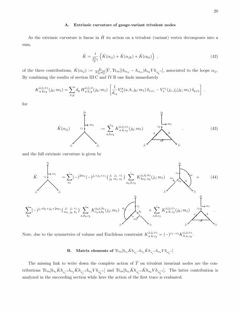
A. Extrinsic curvature of gauge-variant trivalent nodes
As the extrinsic curvature is linear in H its action on a trivalent (variant) vertex decomposes into a
sum,
K =i
l2pγ
(K(αij) + K(αjk) + K(αki)
), (42)
of the three contributions, K(αij) := 4iN2mκl
2p[V ,Trm[(hαij − hαji)hskV hs−1
k], associated to the loops αij .
By combining the results of section III C and IVB one finds immediately
Kjijj ;c1a b;c2
(jk;m1) =∑x,y
dyHjijj ;xa b; y (jk;m1)
[1
dc2V yc2(a, b, jk;m1) δx,c1 − V c1
x (ji, jj |jk;m1) δy,c2
].
for
K(αij)
ji jj
jk
m1c1 :=
∑a,b,c2
Kjijj ;c1a b; c2
(jk;m1)
ji jj
jk
m1c2
a b
m
. (43)
and the full extrinsic curvature is given by
K
ji jj
jk
m1c1 =
∑a1
(−)2m1(−)ji+jj+c1{ ji jj c1jk m1 a1
}∑a2,b,c2
Kjjjk;a1bc2; a2
(ji;m1)
ji jj
jk
m1a2
c2
b
m+ (44)
∑b1
(−)ji+b1+jk+2m1{ ji jj c1m1 jk b1
}∑a,b2,c2
Kjkji;b1c2 a;b2
(jj ;m1)
ji jj
jk
m1
b2
c2
a
m+∑a,b,c2
Kjijj ;c1a b; c2
(jk;m1)
ji jj
jk
m1c2
a b
m
.
Note, due to the symmetries of volume and Euclidean constraint Kjijj ;c1a b; c2
= (−)c1−c2Kjjji;c1b a; c2
.
B. Matrix elements of Trm[hsiKhs−1ihsj Khs−1
jhskV hs−1
k]
The missing link to write down the complete action of T on trivalent invariant nodes are the con-
tributions Trm[hsiKhs−1ihsjKhs−1
jhskV hs−1
k] and Trm[hsiKhs−1
iKhskV hs−1
k]. The latter contribution is
analyzed in the succeeding section while here the action of the first trace is evaluated.

21
The term hsk V hs−1k
is just the same as for the Euclidean Hamiltonian. Therefore,
ji jj
jk
hs−1jhsk V hs−1
k−−−−−−−−−→∑c1,b1
∑c2
(−)2(jk+jj) V jkc2 (ji, jj |c1;m)
ji
−−
jj
−−jk
m
m
c2
c1
jj b1
m
. (45)
Before acting with K the dashed leg m must be erased from the diagram and m moved to the
appropriate place. This can be done simultaneously via (26), (27) and (28) so that K acts on the above
expression by
∑c1,b1
∑c2
V jkc2 (ji, jj |c1;m)
[ ∑a1,b2c3,c4
(−)ji−jj−jk
{c1 c2 m
c3 jk m
}{ji jj c2
m c3 b1
}Kjib1;c3a1b2;c4
(jk;m)
ji
−jj
jk
m
m
c4
b1
b2a1
m
+∑a1,a2b2,c3
(−)ji+a1+c1+c2
{c1 c2 m
ji a1 jj
}{a1 jj c1
m jk b1
}Kb1jk;a1b2c3;a2
(ji;m)
ji
−jj
jk
m
m
c3
b1b2
a2
m
+∑a1,c3b2,b3
(−)jj+b2
ji b2 jk
jj b1 m
c2 m c1
Kjkji;b2c3a1;b3
(jj ;m)
ji
−jj
jk
m
m
c3
b1
b3
a1
m]
In the next step hs−1ihsj is added. For the third term this is straightforward: hsj transforms b1 into a
dashed line and hs−1i
can be coupled as usual via (21) resulting in
∑· · ·∑a2
−−
jj
m
−
ji
m
jk
c3m
a1
a2
a1
b3b1
. (46)

22
The most efficient way to proceed with the other two terms is to couple hsj via (17) and then use (25).
This yields
∑· · ·∑a2,b3
(−)2(a1+b2)−−
ji
m −−
jj
jk
mc4
m
b2
b3
b2
b1
a1
a2a1
=∑· · ·∑a2,b3
(−)jj+c4−a1{ b1 b2 mb3 jj m}{ a1 b2 c4b3 a2 m
}−
ji jj
jk
m
m
c4a2
a1b3
m
(47)
for the first term and
∑· · ·∑a3,b3
(−)2(ji+b3)−
−
−ji
m
m
−−
jj
jk
c3m
b2
b3b2
b1
a1ji
a3
=∑· · ·∑a3,b3
(−)2(ji+b3)(−)b1+b3{ b1 b2 mb3 jj m}
−
ji
m
m
−
jj
jk
c3m
b2
b3
a2
ji
a3
(48)
for the second term. Since the newly created nodes are coplanar, V as well as K are vanishing on them
no matter if they are gauge invariant or not. Therefore it suffices to calculate Tr[hsiK · · · on the inner
parts. E.g. instead of considering the full diagram (47) it suffices to evaluate Tr[hsiK · · · on
−a1 b3
jk
m
m
c4a2
.
Inserting (44) and contracting with the last holonomy hsi results in
∑a3,a4b4,c5
(−)2a4Ka2b3;c4a3b4;c5
(jk;m)−
−a1 b3
−
jk
c5
m
a3 b4a4
a2
+∑a3,a4b4,c5
(−)a2+b3+c4+2m
{a2 b3 c4
jk m a3
}Kb3c4;a3b4c5;a4
(a2;m)
−a1 b3
jk
c5m
a4
a2
m b4
+∑a3,a4b4,b5,c5
(−)2(m+a3)(−)a2+b4+jk
{a2 b3 c4
m jk b4
}Kjka2;b4c5a3;b5
(b3;m) −
a1 b3
jk
c5m
b5a3
a4a3a2
m
.
for this node. Finally, all dashed parts of the graphics can be erased due to (25) and (23). The other
summands, (46) and (48) can be treated along the same lines. Just that in this case the inner parts are
of the same type as the node shown on the right hand side of (45). Consequently, they have to be exerted

23
again to remove the dashed line m and move m to the right place before acting with K. The final
result of this computation is:
Trm[hsiKhs−1ihsjKhs−1
jhskV hs−1
k]
ji jj
jk
=∑b1,c1
∑c2
V jkc2 (ji, jj |c1;m)
[∑
a1,a2,b2b3,c3,c4
(−)ji−a1+c4−jk{ c1 c2 mc3 jk m }{ji jj c2m c3 b1
}Kjib1;c3a1b2;c4
(jk;m){ b1 b2 mb3 jj m}{ a1 b2 c4b3 a2 m
}[
∑a3,a4b4,c5
Ka2b3;c4a3b4;c5
(jk;m)(−)a2+a3−a4+b4+c5{ a2 a3 ma4 a1 m }{ a3 b4 c5jk m a4}
ji jj
jk
a4
a1
b4
b3m
m
+∑a3,b4c5
(−)b3+c4−a2{ a1 a3 mjk c4 b3 }Kb3jk;a3b4c5;a1
(a2;m)
ji jj
jk
a1
c5
b4 b3
m
m
+∑a3,a4b4,b5,c5
(−)a1+a2−a3+a4(−)b3+b4+jk+c5{ b3 b4 mjk c4 a2
}Kjka2;b4c5a3;b5
(b3;m){ a2 a3 ma4 a1 m }{ a3 b5 c5b3 a4 m}
ji jj
jk
a4a1
c5
b3
m
m
]
+∑a1,a2b2,b3,c3
(−)a1−ji+b1−b3+c1+c2{ c1 c2 mji a1 jj }{a1 jj c1m jk b1
}Kb1jk;a1b2c3;a2
(ji;m){ b1 b2 mb3 jj m}[
∑a3,a4b4,c4,c5
(−)a3−a4+a5+b4+c5{ a2 b2 c3c4 m ji}{ ji b2 c4b3 a2 m
}Ka3b3;c3a4b4;c4
(c3;m){ a3 a4 ma5 ji m }{ a4 b4 c5c3 m a5 }
ji jj
jk
a5
c3
b4
b3m
m
+∑a3,a4b4,c4
(−)ji−a2+a4+b2+c3{ ji a2 ma4 a3 m }{ji b2 c4b3 a4 m
}Kb3c3;a4b4c4;a1
(a3;m)
ji jj
jk
c3
c4
b4
b3
m m
+∑a3,a4b4,b5,c4
(−)a2+a4−a5+b2+c4
{b2 m b3c3 a3 b4a2 ji m
}Kc3a3;b4c4a4;b5
(b3;m){ a3 a4 ma5 ji m }{ a4 b5 c4b3 a5 m}
ji jj
jk
c3
c4
b3a5
m m]

24
+∑a1,a2b2,b3,c3
(−)b1−b2+m
{ji b2 jkjj b1 mc2 m c1
}Kjkji;b2c3a1;b3
(b1;m)[
∑a3,a4b4,c4,c5
(−)a2−a3+a4+jj+b3+b4+c3+c4+c5+m{ a1 b3 c3m c4 b1}{ a1 b1 c4jj a2 m
}Ka2jj ;c4a3b4;c5
(c3;m){ a2 a3 ma4 a1 m }{ a3 b4 c4c3 m a4 }
ji jj
jk
a4
c3
b4
a1m
m
+∑a3,c4
(−)a2+b3−c3+m
{jj b1 mc3 b3 a1a3 m a2
}Kjjc3;a3b4c4;a1
(a2;m)
ji jj
jk
c3
c4
b4a1
mm
+∑a3,a4b4,b5,c4
(−)a4−a3+jj−b1+c3+c4+m{ b1 b3 mb4 jj m}{ a1 b3 c3b4 a2 m
}Kc3a2;b4c4a3;b5
(jj ;m){ a2 a3 ma4 a1 m }{ a3 b5 c4jj a4 m}
ji jj
jk
c3
c4
a1
a4
mm]]
C. Computation of Trm[hsiKhs−1iKhskV hs−1
k]
As before hsk V hs−1k
produces a double non-invariant node transforming in the representation H∗m⊗Hmwhere ∗ denotes the adjoint. In contrast to the above the extrinsic curvature K is directly acting on this
node. Therefore it is advisable to introduce an artificial coupling as it was done for the volume:
ji jj
jk
hsk V hs−1k−−−−−−→
∑c1,c2
dc1(−)2jkV jkc2 (ji, jj |c1;m)
ji jj
−
jk
m
mc1
c2
=∑c1,m1
∑c2
V jkc2 (ji, jj |c1;m)(−)c1+c2+m
{m m m1
jk c2 c1
}ji jj
−
jkm
m
m1
c1
Recall that m and m1 are purely internal so that the curvature operator only registers a trivalent node
transforming in spin m1 and the previous results (44) can be employed. Thus hs−1iK is transforming the
above expression into
∑c1,m1
∑c2
V jkc2 (ji, jj |c1;m)(−)c1+c2+m
{m m m1
jk c2 c1
}∑a1,a2b1,c3
Kjijj ;c2a1b1;c3
(jk;m1)(−)2a1−
ji jj
−
jk
− m1m
m
c3
m
a2
a1 b1
m
a1
+ · · ·
.

25
The link m1 can be decoupled and parts of the internal lines can be removed:
−a2 b1
−
jk
−m
c3
a1
m =∑c3
(−)2c4
−a2 b1
−
−
−
jk
c3
a1
m
c4
−m c3
=∑c4
(−)2c4(−)b1+jk−a1
{a1 b1 c3
c4 m a2
}{m m m1
jk c3 c4
}a2 b1
jk
mc4
The rest of the calculation is completely equivalent to the one in the previous section. With all other
terms one can proceed similarly resulting in:
∑c1,m1
∑c2
V jkc2 (ji, jj |c1;m)(−)c1+c2+m{m m m1
jk c2 c1 }[ ∑a1,a2b1,c3
Kjijj ;c2a1b1;c3
(jk;m1)[
∑a3,a4b2,c4,c5
(−)a3+a4+m(−)b2−b1+jk+c5+m1{ a1 b1 c3c4 m a2 }{ jk c3 m1m m c4 }K
a2b1;c4a3b2;c5
(jk;m){ a2 a3 ma4 a1 m }{ a3 b2 c5jk m a4}
ji jj
jk
a4
a1
b2
b1m
m
+∑a3,b2c4
(−)a1+a2+a3+b1+c3+m{ a1 m1 a3m a2 m }{ a1 m1 a3
jk b1 c3 }Kb1jk;a3b2c4;a1
(a2;m)
ji jj
jk
a1
c4
b2 b1
m
m
+∑a3,a4b2,b3,c4
(−)a2+a3+a4+b1−jk+c3+c4+m{a1 b1 c3a2 b2 jkm m m1
}Kjka2;b2c4a3;b3
(b1;m){ a2 a3 ma4 a1 m }{ a3 b2 c5jk m a4}
ji jj
jk
a4a1
c4
b1
m
m
]

26
∑a1,a2,a3b1,c3
(−)a2+a3−ji+jj+c2+m{ ji jj c2jk m1 a1
}Kjjjk;a1b1c3;a2
(ji;m1){ ji a2 m1m m a3 }
[ ∑a4,a5b2,c4,c5
(−)2m(−)a4+a5+b1+b2+c4+c5{ a2 b1 c3c4 m a3 }Ka3b1;c4a4b2;c5
(c3;m){ a3 a4 ma5 ji m }{ a4 b2 c5c3 m a5 }
ji jj
jk
a5
c3
b2
b1m
m
+∑b4,c2
(−)2jiKb1c3;a2b2c4;ji
(a3;m)
ji jj
jk
c3
c4
b2
b1
m m
+∑a4,a5b2,b3,c4
(−)ji+a2+a4+a5−c3+c4{ a2 b1 c3b2 a3 m}Kc3a3:b2
c4a4;b3(a2;m){ a3 a4 ma5 ji m }{ a4 b3 c4b1 a5 m
}
ji jj
jk
c3
c4
b1a5
m m]
+∑a1,a2b1,b2,c3
(−)ji+jk+b1{ ji jj c2m1 jk b1
}Kjkji;b1c3a1;b2
(jj ;m1)
[ ∑a3,a4b3,c4,c5
(−)2jj (−)m−a2+a3+a4+b3+c3+c4+c5
{a1 c3 b2a2 c4 jjm m m1
}Ka2jj ;c4a3b3;c5
(c3;m){ a2 a3 ma4 a1 m }{ a3 b3 c5c4 m a4 }
ji jj
jk
a4
c3
b3
a1m
m
+∑a3,b3c4
(−)jj+c3−a2−m{ a1 m1 a3m a2 m }{ a1 m1 a3
jj c3 b2 }Kjjc3;a3b3c4;ji
(a2;m)
ji jj
jk
c3
c4
b3a1
mm
+∑a3,a4b3,b4,c4
(−)a3−a4+b2−b3−c3+c4+m1+m{ a1 b2 c3b3 a2 m}{ b2 jj m1
m m b3}Kc3a2;b3
c4a3;b4(jj ;m){ a2 a3 ma4 a1 m }{ a3 b4 c4jj a4 m
}
ji jj
jk
c3
c4
a1
a4
mm]]
D. Contraction with ε
To obtain the full action of T on a trivalent (invariant) node both trace contributions as computed in the
previous sections must be summed up and contracted with the ε-tensor. For the Euclidean constraint this
antisymmetric contraction could be nicely absorbed in the loop trick (36) and lead to major simplifications.
Unfortunately, this does not happen for the remaining part of the scalar constraint. Since both, volume

27
and extrinsic curvature, depend on whether one couples first holonomy hk or hi this contraction is not
simplifying but complicating matters.
Yet, since we used an abstract calculus to evaluate the trace parts we are free to switch edges and nodes in
the most advantageous position as long as the changes in (abstract) orientation and ordering are respected.
For example:
Tr[hsjKhs−1jhsiKhs−1
ihsk V hs−1
k]
ji jj
jk
= (−)ji+jj+jk Tr[hsjKhs−1jhsiKhs−1
ihsk V hs−1
k]
jj ji
jk
The trace can now be evaluated as above treating i as j and j as i. Finally the edges should be flipped
back:
Tr[hsjKhs−1jhsiKhs−1
ihsk V hs−1
k]
ji jj
jk
= (−)ji+jj+jk∑a1,c1
∑c2
(−)jk−c2V jkc2 (ji, jj |c1;m)
[
∑b1,b2,a2a3,c3,c4
(−)jj−b1+c4−jk{ c1 c2 mc3 jk m }{ jj ji c2m c3 a1}(−)c3−c4K
a1jj ;c3a2b1;c4
(jk;m){ a1 a2 ma3 ji m }{ b1 a2 c4a3 b2 m }[
∑b3,b4a4,c5
(−)c4−c5Ka3b2;c4a4b3;c5
(jk;m)(−)b2+b3−b4+a4+c5{ b2 b3 mb4 b1 m}{ b3 a4 c5jk m b4
}(−)jk+jj+ji
ji jj
jk
a4
a1
b4
b3m
m
+ · · ·]
+ · · ·]
where we used V jkc2 (ji, jj |c1;m) = (−)jk−c2V jk
c2 (jj , ji|c1;m), Ka1jj ;c3a2b1;c4
= (−)c3−c4 and
jj ji
jk
b4
b1
a4
a3m
m
= (−)jk+a4+b4(−)b4+b1+m(−)jj+b1+m(−)a4+a3+m(−)ji+a3+m︸ ︷︷ ︸(−)jk+jj+ji
ji jj
jk
a4
a1
b4
b3m
m
.
Note, that here the sign generated by the first switch of the edges is canceled by the one originating from
restoring the old orientations. This is a generic property and applies to all terms of the full expression.
Only signs arising from volume and extrinsic curvature remain. The matrix elements corresponding to
cyclic permutations of (i, j, k) are simply obtained by exchanging the labels (ji, a.) by (jj , b.), (jj , b.) by
(jk, c.) and so forth.
The second contribution Tr[hsiKhs−1iKhsk V hs−1
k] can be treated along the same lines. The value of
Tr[hsjKhs−1jKhsk V hs−1
k] can be calculated by first flipping the edges so that i can be treated as j and
vice versa and afterwards restoring the original orientation.

28
VI. CONCLUSION AND OUTLOOK
In this article we derived for the first time an explicit formula for the matrix elements of the full
Hamiltonian constraint in LQG including the Lorentzian part. As already pointed out, this constraint
plays a major role in any canonical quantization program for GR based on real Ashtekar-Barbero variables
so that the methods developed in the course of the calculation are also of interest in these approaches,
e.g. the master constraint approach. On the other hand, the tools developed to compute the action of
the curvature (especially the loop trick (36)) or extrinsic curvature can be easily adapted to models with
non-graph changing operators, as the extended master constraint ansatz or AQG, by extending the loops
involved in the regularization in such a way that no new links are created.
By exploiting several new recoupling identities, we significantly simplified the matrix element so that
the recoupling part is totally captured in 6j and 9j symbols for which symmetry properties and explicit
formulas are well known. Of course the final expression still depends on the volume but can be easily
implemented on a computer for further investigations. We also expect to get interesting insight from
a large j expansion or the application in symmetry reduced models. Of special interest would be for
example the recently introduced model [38, 39] which keeps the original SU(2) structure of the theory
but has a diagonal volume operator so that it may be possible to give an analytical closed formula for
the whole constraint within this Ansatz. Finally the presented analysis opens the way for a comparison
with the covariant approach, because the spin foam vertex amplitudes are expected to be annihilated by
the Hamiltonian constraint [27]. As the matching between the canonical and covariant kinematics [40] led
to the upgrade of the old Barret-Crane model [41] to the new EPRL-model [42], the matching with the
dynamical constraint is expected to shed new light onto the canonical-covariant joint theory.
ACKNOWLEDGMENTS
The authors wish to thank T.Thiemann for useful discussions and L.Cottrell for a careful reading of the
manuscript. The work of E.A. was partially supported by the grant of Polish Narodowe Centrum Nauki
nr DEC-2011/02/A/ST2/00300. A.Z. acknowledges financial support of the ’Elitenetzwerk Bayern’ on the
grounds of ’Bayerische Eliteförder Gesetz’.
Appendix A: More on 3j’s, 6j’s and 9j’s
For self-containedness some important properties of nj-Symbols are listed here. Introductions to Recou-
pling theory can be found in various textbooks on quantum mechanics and quantum angular momentum,
e.g. [37]. For an extensive list of properties of nj-symbols see e.g. [43]
3j-Symbols

29
Relation to Clebsh-Gordan coefficients:
〈a, α; b, β|c, γ〉 = (−)b−a+γ√
2c+ 1
(a b c
α β −γ
)
where |b, β; a, α〉 = |b, β〉 ⊗ |a, α〉
Compatibility criteria
If one (or several) of the following rules is violated, then
(a b c
α β γ
)is vanishing:
∗ a, b, c ∈ 12N, a± α ∈ N, −a ≤ α ≤ a, · · ·
∗ α+ β + γ = 0
∗ a+ b+ c ∈ N, |a− b| ≤ c ≤ a+ b (triangle inequality)
Symmetries(a b c
α β γ
)= (−)a+b+c
(a b c
−α −β −γ
)= (−)a+b+c
(b a c
β α γ
)=
(b c a
β γ α
)
6j-Symbols
Definition in terms of 3j’s{j1 j2 j3
j4 j5 j6
}=
∑µ1,··· ,µ6
(−)
6∑i=1
(ji−µi)(j1 j2 j3
µ1 µ2 −µ3
)(j1 j5 j6
−µ1 µ5 µ6
)(j4 j5 j3
µ4 −µ5 µ3
)(j4 j2 j6
−µ4 −µ2 −µ6
)
Symmetries{a b c
d e f
}=
{b a c
e d f
}=
{b c a
e f d
}=
{d e c
a b f
}=
{d b f
a e c
}=
{a e f
d b c
}
Compatibility{a b c
d e f
}= 0 unless the triangle inequalities hold for {a, b, c}, {a, e, f}, {d, b, f} and {d, e, c}
Orthogonality
∑x
dx
{a b x
d e c
}{a b x
d e c′
}= δc,c′
1
dc
if the compatibility requirements are fulfilled.
9j-Symbols

30
Definition by 3j’sj1 j2 j3
j4 j5 j6
j7 j8 j9
=∑
µ1,...,µ9
(−)
9∑i
(ji−µi)(j1 j2 j3
µ1 µ2 µ3
)(j4 j5 j6
µ4 µ5 µ6
)(j7 j8 j9
µ7 µ8 µ9
)
×(j1 j4 j7
−µ1 −µ4 −µ7
)(j2 j6 j8
−µ2 −µ6 −µ8
)(j3 j6 j9
−µ3 −µ6 −µ9
)
Definition by 6j′sa f r
d q e
p c b
:=∑x
dx(−1)2x
{a b x
c d p
}{c d x
e f q
}{e f x
a b r
}
Symmetriesa f r
d q e
p c b
= (−)S
d q e
a f r
p c b
= (−)S
a f r
p c b
d q e
= (−)S
f a r
q d e
c p b
= (−)S
a r f
d e q
p b c
where S = a+ b+ c+ d+ e+ f + p+ q + r.
Appendix B: Volume
For the sake of completeness the volume operator is briefly reviewed and the graphical framework for
computing the action is discussed here, closely following [32] and [29]. Thereby we restrict our attention
to the Ashtekar-Lewandowski volume [31], which was also analyzed in greater detail in [34].
1. General properties
Let Ts be a cylindric function on a spin network s and let V(Γ) denote the set of nodes of the underlying
graph Γ. The volume operator V acts on Ts by
V Ts =∑
v∈V(Γ)
Vv Ts , (B1)
where
Vv = l3p
√√√√∣∣∣∣∣ i
16 · 3!
∑eI∩eJ∩eK=v
ε(eI , eJ , eK)W[IJK]
∣∣∣∣∣ . (B2)

31
The sum extends over all triples (eI , eJ , eK) of edges adjacent to the vertex v, lp denotes the Planck
length and ε(eI , eJ , eK) is determined by the orientation of the tangents eI at v, i.e. ε(eI , eJ , eK) =
sgn[det(eI , eJ , eK)]. The grasping operator
W[IJK] := εijkXiIX
jJX
kK (B3)
depends on the right invariant vector fields (of SU(2))
XiI := −iTr
[(heIσ
i)T∂
∂heI
](B4)
along the edge eI at v. Here, eI was chosen to be outgoing of v, σi are the Pauli matrices and T denotes the
transpose. The matrix elements [σi]AB with spinorial indices A,B = 0, 1 and vector indices i = 1, 2, 3 are
natural intertwiners of spin and vector representation (i.e. (1, 1/2, 1/2)). Thus, XiI inserts an intertwiner
[σi]AB at an edge labeled by the fundamental representation. Since an irrep l is the completely symmetrized
tensor product of 2l fundamental representations this can be immediately generalized to edges labeled by
l. Similarly ε is a vector invariant intertwining (1, 1, 1). Following the spirit of the graphical calculus,
W[IJK] can be visualized by
√3!
1 1 1 (B5)
where each handle grasps an edge e at v. Note, this grasping depends on the orientation of e. Yet, we want
to use 3j-symbols rather then the invariants σ and ε. These differ from the corresponding 3j’s by a normal-
ization constant. I.e. the 3j’s are normalized to one while Tr[ε2] = 3! and∑
i Trl[(σi)2] = 4[l(l+1)(2l+1)]
where Trl indicates that the trace is evaluated in spin l. Thus,√
3! in (B5) stems from the normalization of
ε. Each grasp of an edge colored by l gives additionally a factor Nl := −i2√l(l + 1)(2l + 1), in particular
1
l = Nl ·+
1
l . (B6)
When using this formalism12, one should keep in mind that the right invariant vector fields are derivative
operators and hence only act on true holonomies. On the other hand W can not change the graph itself
but only alter the intertwiners. Consequently, the links in (B5) are only added at the vertex (in a dashed
environment) and can be erased again by pure recoupling theory.
12 This was developed first in [32]. However, they used another calculus based on Temperley-Lieb algebras which yields
different normalizations.

32
2. Trivalent nodes
The computational effort to determine the matrix elements of the volume operator is increasing heavily
with the valency of the nodes. Therefore we only discuss the case of a trivalent node
|vx〉 :=
ji jj
jk
mx (B7)
transforming in spin m. On a trivalent node Vv reduces to l3p4
√∣∣iWijk]
∣∣ and the grasping yields
√3!
ji jj
jk
mx
=√
3!NjkNjiNjj
∑y
dy
− −
x
jk
−
−y
jj
jkm
jijijj
ji jj
jk
my . (B8)
In the second step a resolution of the identity in the intertwiner space was inserted (see section III B). A
careful evaluation by the usual methods reveals that
− −
x
jk
−
−y
jj
jkm
jijijj
= (−)x+jk−m
{jk jk 1
x y m
}ji 1 ji
x 1 y
jj 1 jj
. (B9)
The 6j in this equation is only non-zero if (x, y, 1) obey the triangle inequality, i.e. if |x− y| ≤ 1. But for
x = y the 9j-symbol is vanishing since it is anti-symmetric when switching first and last column. On the
other hand, the 6j and the 9j are symmetric under the exchange of x and y for y = x ± 1. Thus, if we
work with rescaled nodes |vx〉N =√dx|vx〉 then
W[IJK]|vx〉N =∑y
W xy|vy〉N
yields an antisymmetric matrix W which has only sub- and super-diagonal non-zero entries:
W xy = δy,x±1
√3!√dxdyNjkNjiNjj (−)x+jk−m
{jk jk 1
x y m
}ji 1 ji
x 1 y
jj 1 jj
. (B10)
Fortunately, this matrix is diagonalizable so that the square root ofW has a well-defined meaning. Suppose
U is the (unitary) map that maps {|vx〉N} to the eigenbasis of W then the matrix elements of the volume
(compare with (32)) are finally given by
V xy(ji, jj |jk;m) =
l3p4
√dydx
[U−1]x w
√|i[WD]w zU
zy Λ (B11)

33
where WD = UWU−1 is the diagonalized matrix. For small m the intertwiner space is low dimensional
and this diagonalization does not cause much problems:
m = 0: For m = 0 the intertwiner space is one-dimensional and therefore V annihilates gauge-invariant
trivalent nodes.
m = 12 : Here, the intertwiner space is 2-dimensional and it is not hard to check that V is diagonal with
matrix elements
V xy(ji, jj , jk|
1
2) = δxy
l3p4
[|i√
3!√djk+ 1
2djk− 1
2NjkNjiNjj{
jk jk 1
jk+ 12jk− 1
212}{
ji 1 jijk+ 1
21 jk− 1
2jj 1 jj
}|]− 1
2
.
m = 1: For m = 1 W is a 3× 3-matrix but does not have full rank. Nevertheless, it is diagonalizable when
applying first a similarity transformation S (see [34]):
W =
0 w1 0
−w1 0 w2
0 −w2 0
S−→
0 1
w1λ2 0
−w1 0 0
0 −w2w1
0
U−−→ λ
−i 0 0
0 i 0
0 0 0
−−→ V =l3p4
|w1|2λ 0 − |w1 w2|2
λ
√2jk+32jk−1
0 λ 0|w1 w2|2
λ
√2jk−12jk+3
|w2||w1|
|w2|2λ
where
w1 = (−)2(jk−1)√
3!√djk−1 djk NjkNjiNjj{
jk jk 1
jk−1 jk12}{
ji 1 jijk−1 1 jkjj 1 jj
}
w2 = (−)2jk−1√
3!√djk+1 djk NjkNjiNjj{
jk jk 1
jk+1 jk12}{
ji 1 jijk+1 1 jkjj 1 jj
}and λ2 = |w1|2 + |w2|2.
[1] A. Ashtekar, “New variables for classical and quantum Gravity", Phys. Rev. Lett. 57, 2244-2247 (1986).[2] J. F. Barbero, “Real Ashtekar variables for Lorentzian signature space times", Phys. Rev. D51, 5507-5510
(1995).[3] A.Ashtekar, J. Lewandowski, “Background independent quantum gravity: A status report”, Class.Quant.Grav.
21 R53 (2004).[4] T.Thiemann, “Modern canonical quantum general relativity”, (Cambridge University Press, Cambridge, UK,
2007).[5] C.Rovelli, “Quantum Gravity", (Cambridge University Press, Cambridge 2004).

34
[6] P. Dirac, “Lectures on Quantum Mechanics", (Belfer Graduate School of Science, Yeshiva University Press,NewYork 1964).
[7] C. Rovelli and L. Smolin, “Spin networks and quantum gravity,” Phys. Rev. D 52 (1995) 5743.[8] R. Penrose, “Angular momentum: an approach to combinatorial space-time", in Quantum theory and beyond,
T. Bastin ed., Cambridge Univ. Press., New York (1971)[9] A. Ashtekar, J. Lewandowski, D. Marolf, J. Mourao and T. Thiemann, “Quantization of diffeomorphism
invariant theories of connections with local degrees of freedom,” J. Math. Phys. 36, 6456 (1995).[10] T. Thiemann, “Anomaly - free formulation of nonperturbative, four-dimensional Lorentzian quantum gravity,”
Phys. Lett. B 380, 257 (1996).[11] C. Rovelli, “Ashtekar formulation of general relativity and loop space nonperturbative quantum gravity: A
Report,” Class. Quant. Grav. 8, 1613 (1991).V. Husain, “Intersecting loop solutions of the hamiltonian constraint of quantum general relativity” Nucl. Phys.B 313, 711 (1989).B. Bruegmann, J. Pullin, “Intersecting N loop solutions of the Hamiltonian constraint of quantum gravity,”Nucl. Phys. B 363, 221 (1991).R. Gambini, “Loop space representation of quantum general relativity and the group of loops,” Phys. Lett. B255, 180 (1991).B. Bruegmann, R. Gambini, J. Pullin, “Jones polynomials for intersecting knots as physical states of quantumgravity,” Nucl. Phys. B 385, 587 (1992). C. Rovelli, L. Smolin, “The Physical Hamiltonian in nonperturbativequantum gravity,” Phys. Rev. Lett. 72, 446 (1994)
[12] T. Thiemann, “Quantum spin dynamics (QSD),” Class. Quant. Grav. 15, 839 (1998).[13] T. Thiemann, “Quantum spin dynamics (QSD) II,” Class. Quant. Grav. 15, 875 (1998).[14] R. Gambini, J. Lewandowski, D. Marolf, J. Pullin, “On the consistency of the constraint algebra in spin network
quantum gravity,” Int. J. Mod. Phys. D 7, 97 (1998).J. Lewandowski, D. Marolf, “Loop constraints: A habitat and their algebra,” Int. J. Mod. Phys. D 7, 299(1998).L. Smolin, “The classical limit and the form of the Hamiltonian constraint in non-perturbative quantum generalrelativity,” [arXiv:gr-qc/9609034].
[15] T. Thiemann, “The Phoenix project: Master constraint programme for loop quantum gravity,” Class. Quant.Grav. 23, 2211 (2006),B. Dittrich and T. Thiemann, “Testing the master constraint programme for loop quantum gravity. I: Generalframework,” Class. Quant. Grav. 23, 1025 (2006)T. Thiemann, “Quantum spin dynamics. VIII: The master constraint,” Class. Quant. Grav. 23, 2249 (2006)
[16] K. Giesel and T. Thiemann, “Algebraic Quantum Gravity (AQG) I. Conceptual Setup,” Class. Quant. Grav.24, 2465 (2007)K. Giesel and T. Thiemann, “Algebraic Quantum Gravity (AQG). II. Semiclassical Analysis,” Class. Quant.Grav. 24, 2499 (2007)K. Giesel and T. Thiemann, “Algebraic quantum gravity (AQG). III. Semiclassical perturbation theory,” Class.Quant. Grav. 24, 2565 (2007)K. Giesel and T. Thiemann, “Algebraic quantum gravity (AQG). IV. Reduced phase space quantisation of loopquantum gravity,” Class. Quant. Grav. 27, 175009 (2010)

35
[17] M. Domagala, K. Giesel, W. Kaminski and J. Lewandowski, “Gravity quantized: Loop Quantum Gravity witha Scalar Field,” Phys. Rev. D 82, 104038 (2010) [arXiv:1009.2445 [gr-qc]].
[18] K. Giesel and T. Thiemann, “Scalar Material Reference Systems and Loop Quantum Gravity,” arXiv:1206.3807[gr-qc].
[19] V. Husain and T. Pawlowski, “Time and a physical Hamiltonian for quantum gravity,” Phys. Rev. Lett. 108,141301 (2012)
[20] A. Ashtekar and P. Singh, “Loop Quantum Cosmology: A Status Report,” Class. Quant. Grav. 28, 213001(2011)
[21] M. Bojowald, “Loop quantum cosmology,” Living Rev. Rel. 11, 4 (2008).[22] A. Perez, “The Spin Foam Approach to Quantum Gravity,” Living Rev. Rel. 16, 3 (2013)
A. Perez, “Spin foam models for quantum gravity,” Class. Quant. Grav. 20, R43 (2003).J. Baez, “An introduction to Spinfoam Models of BF Theory and Quantum Gravity", Lect.Notes Phys. 543,25-94 (2000).C. Rovelli, “Zakopane lectures on loop gravity", (2011), [arXiv:gr-qc/1102.3660].
[23] M. P. Reisenberger, C. Rovelli, “*Sum over surfaces* form of loop quantum gravity,” Phys. Rev. D 56, 3490(1997).
[24] K. Noui, A. Perez, “Three dimensional loop quantum gravity: Physical scalar product and spin foam models,”Class. Quant. Grav. 22, 1739 (2005).E. Alesci, K. Noui, F. Sardelli, “Spin-Foam Models and the Physical Scalar Product,” Phys. Rev. D 78, 104009(2008).B. Bahr, “On knottings in the physical Hilbert space of LQG as given by the EPRL model", Class. Quant.Grav. 28, 045002 (2011), [arXiv:gr-qc/1006.0700].
[25] E. Alesci, “Regularized Hamiltonians and Spinfoams,” J. Phys. Conf. Ser. 360 (2012) 012041[26] E. Alesci, C. Rovelli, “A Regularization of the hamiltonian constraint compatible with the spinfoam dynamics",
Phys. Rev. D 82, 044007 (2010).[27] E. Alesci, T. Thiemann and A. Zipfel, “Linking covariant and canonical LQG: New solutions to the Euclidean
Scalar Constraint,” Phys. Rev. D 86, 024017 (2012) [arXiv:1109.1290 [gr-qc]].[28] R. Borissov, R. De Pietri, C. Rovelli, “Matrix elements of Thiemann’s Hamiltonian constraint in loop quantum
gravity,” Class. Quant. Grav. 14, 2793 (1997).[29] M. Gaul, C. Rovelli, “A generalized Hamiltonian constraint operator in loop quantum gravity and its simplest
Euclidean matrix elements,” Class. Quant. Grav. 18, 1593 (2001).[30] C. Rovelli, L. Smolin, “Discreteness of area and volume in quantum gravity,” Nucl. Phys. B 442, 593 (1995)
[Erratum-ibid. B 456, 753 (1995)].[31] A. Ashtekar, J. Lewandowski, “Quantum theory of geometry. II: Volume operators,”
Adv. Theor. Math. Phys. 1, 388 (1998), [arXiv:gr-qc/9711031].J. Lewandowski, “Volume and quantizations,” Class. Quant. Grav. 14, 71 (1997).
[32] R. De Pietri, C. Rovelli, “Geometry Eigenvalues and Scalar Product from Recoupling Theory in Loop QuantumGravity,” Phys. Rev. D 54, 2664 (1996), [arXiv:gr-qc/9602023].
[33] T. Thiemann, “Closed formula for the matrix elements of the volume operator in canonical quantum gravity,”J. Math. Phys. 39, 3347 (1998) [gr-qc/9606091].
[34] J. Brunnemann, T. Thiemann, “Simplification of the spectral analysis of the volume operator in loop quantumgravity,” Class. Quant. Grav. 23, 1289 (2006).

36
[35] J. Brunnemann and D. Rideout, “Properties of the volume operator in loop quantum gravity. I. Results,” Class.Quant. Grav. 25, 065001 (2008) [arXiv:0706.0469 [gr-qc]].
[36] J. Brunnemann and D. Rideout, “Properties of the volume operator in loop quantum gravity. II. DetailedPresentation,” Class.Quant.Grav.25:065002,2008
[37] D.M. Brink, G.R. Satchler, “Angular Momentum" 2nd ed., (Clarendon Press, Oxford 1968).[38] E. Alesci and F. Cianfrani, “Quantum-Reduced Loop Gravity: Cosmology,” Phys. Rev. D 87, 083521 (2013) ,
[arXiv:1301.2245 [gr-qc]].[39] E. Alesci and F. Cianfrani, “A new perspective on cosmology in Loop Quantum Gravity,” arXiv:1210.4504
[gr-qc].[40] E. Alesci, C. Rovelli, “The complete LQG propagator: I. Difficulties with the Barrett-Crane vertex,” Phys.
Rev. D 76, 104012 (2007).[41] J. W. Barrett, L. Crane, “Relativistic spin networks and quantum gravity,” J. Math. Phys. 39, 3296 (1998),[42] J. Engle, E. Livine, R. Pereira, C. Rovelli, “LQG vertex with finite Immirzi parameter,” Nucl. Phys. B 799
(2008) 136 .[43] http://functions.wolfram.com/HypergeometricFunctions/ThreeJSymbol/