The tree Constraint

Nicolas Beldiceanu1, Pierre Flener2,3, and Xavier Lorca1

1 École des Mines de Nantes, LINA FREE CNRS 2729,FR-44307 Nantes Cedex 3, France

{Nicolas.Beldiceanu,Xavier.Lorca}@emn.fr2 Department of Information Technology, Uppsala University,

Box 337, SE–751 05 Uppsala, SwedenPierre.Flener@it.uu.se

3 The Linnaeus Centre for Bioinformatics, Uppsala University,Box 598, SE–751 24 Uppsala, Sweden

Abstract. This article presents an arc-consistency algorithm for the treeconstraint, which enforces the partitioning of a digraph G = (V, E) into aset of vertex-disjoint anti-arborescences. It provides a necessary and suf-ficient condition for checking the tree constraint in O(|V| + |E|) time, aswell as a complete filtering algorithm takingO(|V| · |E|) time.

1 Introduction

Graph partitioning constraints were already considered from an early stageof constraint programming research as natural shortcuts for expressing con-straints on a graph. This was for instance the case of the Hamiltonian circuitand spanning tree constraints of ALICE [11]. Later on, this was also the casefor the cycle [3] and path constraints [5,14,15], which were respectively intro-duced in some later version of CHIP [7] and Ilog Solver [12]. But curiously,despite its study within the Operations Research and algorithm design commu-nities [6,13], the problem of partitioning a digraph into a set of vertex-disjointanti-arborescences4 was so far ignored by the constraint programming commu-nity. This problem has a lot of practical applications, for instance in VLSI cir-cuit design. The application that motivated us is the construction of a supertreefrom given trees with overlapping leaf sets, such that the ancestor relationshipsof the given trees are preserved. This is an important issue in phylogeny andhas applications in molecular biology and linguistics [1], such as the construc-tion of the Tree of Life [4]. See the description of future work in Section 4 forhow this phylogenetic problem relates to the problem described here.

This paper addresses the mentioned digraph partitioning problem from aconstraint programming perspective.5 We should stress that, as usual within

4 A digraph A is an anti-arborescence with anti-root r iff there exists a path from all ver-tices of A to r and the undirected graph associated with the digraphA is a tree.

5 The term "tree constraint" exists in the constraint programming community, but thetree processing problem defined in [1] assembles a set of trees in one single tree accord-ing to some dominance constraints.

constraint programming, our goal is not partitioning a given digraph G intovertex-disjoint anti-arborescences, but rather first to find out whether this ispossible at all or not, and second to detect those arcs of G that do not belongto any partitioning. Throughout this article, we use for simplicity the term treerather than the term anti-arborescence.

The tree constraint has the form tree(NTREE, VERTICES), where NTREE is a in-teger variable6 and VERTICES is a collection of n items, each item consisting ofthe following attributes:

- index is an integer between 1 and n.- father is an integer variable whose domain is a subset of the values of the

interval [1, n].

The i-th item of the VERTICES collection is denoted VERTICES[i]. Furthermore,VERTICES[i].attr represents the value of attribute attr of VERTICES[i]. A collec-tion of n items, each having p attributes a1, a2, ..., ap is denoted by:

{(a1 − v11, ..., ap − v1p), (a1 − v21, ..., ap − v2p), ..., (a1 − vn1, ..., ap − vnp)}

In order to define the tree constraint we first introduce the digraph associatedwith any instance of the tree constraint. We then define the meaning of the treeconstraint as a graph property that must hold on the digraph associated with aground7 instance of the tree constraint.

Definition 1. Digraph associated with a tree constraintTo any tree(NTREE, VERTICES) constraint we associate the digraph G = (V , E), where:

- To each item VERTICES[i], (1 ≤ i ≤ n), of the VERTICES collection corresponds avertex of V denoted by vi. Observe that |V| = n.

- For every pair of items (VERTICES[i],VERTICES[j]), where i and j are not nec-essarily distinct, there is an arc from vi to vj in E (i.e., (vi, vj) ∈ E) if j ∈dom(VERTICES[i].father). Let:

m = |E| =n�

i=1

|dom(VERTICES[i].father)|

Observe that each vertex of the digraph G associated with a ground instanceof the tree constraint has exactly one successor.

Definition 2. A ground instance of a tree(NTREE, VERTICES) constraint holds ifVERTICES[i].index = i , (1 ≤ i ≤ n), and if its associated digraph G = (V , E) ver-ifies the two following conditions:

- G consists of NTREE connected components.

6 A integer variable V is a variable that ranges over a finite set of integers denoted bydom(V ). min(V ) and max(V ) respectively denote the minimum and the maximumvalue of V .

7 An instance such that all its integer variables are fixed.

- Each connected component of G does not contain any circuit involving more thanone vertex.

The index and the father attributes of an item can be respectively interpretedas the unique identifier of that item and as the successor of that item in thepartionning into trees.

Fig. 1. (A) A digraph G and (B) three possible vertex-disjoint tree partitionings of G.

Example 1. For the digraph depicted by part (A) of Figure 1, a tree constraint isstated as tree(NTREE, VERTICES) where:

VERTICES = {(index − 1, father − F1), (index − 2, father − F2),(index − 3, father − F3), (index − 4, father − F4),(index − 5, father − F5), (index − 6, father − F6),(index − 7, father − F7), (index − 8, father − F8),(index − 9, father − F9), (index − 10, father − F10),(index − 11, father − F11)},

dom(NTREE), dom(F1), dom(F2), dom(F3), dom(F4), dom(F5), dom(F6), dom(F7),dom(F8), dom(F9), dom(F10), dom(F11) respectively are {1, 2, 3, 4, 5}, {2, 4, 7, 10},{1}, {4, 5, 11}, {3, 4}, {6}, {5, 6}, {8, 11}, {7, 9, 10, 11}, {8, 9, 11}, {8, 9, 10}, {8}.

Part (B) of Figure 1 shows three possible solutions of the vertex-disjoint parti-tioning of G with respectively 2, 3 and 4 trees. Observe that, as stated by thesecond condition of Defintion 2, there is no circuit involving more than onevertex. In order to achieve arc-consistency we have to prune NTREE as well asF1, F2, . . . , F11 in the following way:

– We want to find out that 1 and 5 are not feasible numbers of trees for parti-tioning G, then dom(NTREE) = {2, 3, 4}.

– According to the previous restriction of dom(NTREE), we restrict the do-mains of F1, F6, F8 respectively to dom(F1) = {4, 7, 10}, dom(F6) = {6}and dom(F8) = {9, 10}.

Example 1 will be used throughout this article in order to illustrate the differentpropositions.

The tree constraint was introduced within a catalogue of global constraints[2, page 74] but no filtering algorithm was known. The contribution of this ar-ticle is an O(n ·m) arc-consistency filtering algorithm for the tree constraint.

The rest of the article is organised as follows: Section 2 provides a necessaryand sufficient condition for partitioning the digraph G associated with a treeconstraint according to a given set dom(NTREE) of potential numbers of trees.Section 3 shows how to exploit this necessary and sufficient condition in orderto prune NTREE as well as the father variables. Finally, Section 4 concludes thisarticle and outlines future work.

2 Checking Feasibility

This section first gives a necessary and sufficient condition for the tree constraintto hold. Second, it sketches anO(n+m) algorithm for evaluating that condition.Before presenting it, we introduce some terminology regarding the digraph G =(V , E) associated with a tree constraint, as well as a lower and upper bound onthe number of trees needed for partitioning G:

– To each instance of a tree(NTREE, VERTICES) constraint we associate the re-duced digraph Gr derived from G in the following way: to each strongly con-nected component of G we associate a vertex of Gr; to each arc of G thatconnects different strongly connected components corresponds an arc inGr. A strongly connected component of G that corresponds to a sink of Gr iscalled a sink component.

– A vertex v of G = (V , E) such that (v, v) ∈ E is called a potential root. The arc(v, v) is called a loop. A strongly connected component of G that contains atleast one potential root is called a rooted component.

– A vertex u of G = (V , E) is a door of the strongly connected componentassociated with u iff there exists (u, v) ∈ E such that u and v do not belongto the same strongly connected component of G.

– A connecting arc (u, v) of G = (V , E) is an arc of E such that u and v do not be-long to the same strongly connected component. Similary, a non-connectingarc (u, v) of E is an arc such that u and v belong to the same strongly con-nected component.

– A vertex v of G = (V , E) is a winner if v is a door or if (v, v) ∈ E , i.e., apotential root.

– Enforcing an arc (u, v) of G corresponds to removing from G all arcs (u, w)such that w 6= v.

Example 2. Figure 2 illustrates the previous terms according to the digraph in-troduced in part (A) of Figure 1. In part (A), the winners correspond to the doorsand potential roots. The connecting arcs and the loops are depicted by a black line,while the other arcs are depicted by a dotted line. S2, S3, S4 are rooted compo-nents while S3, S4 are sink components. Part (B) depicts the reduced digraph as-sociated with G. To each strongly connected component Si of G corresponds avertexRi of Gr . Observe that R3 and R4 represent sink vertices.

Fig. 2. (A) The digraph G and its strongly connected components S1, S2, S3, S4. (B) Thereduced digraph Gr associated with G.

We now present a lower and upper bound on the number of trees that canpossibly cover a given digraph G associated with a tree constraint. For this pur-pose, we name by MINTREE the number of sinks of Gr and by MAXTREE the num-ber of potential roots of G.

Proposition 1. A lower bound on the minimum number of trees for partitioning thedigraph G associated with a tree constraint is the number of sinks in Gr (i.e., MINTREE).

Proof. Proposition 1 stems from the fact that there is no path between two ver-tices that belong to two distinct sink components of G. ut

Proposition 2. An upper bound on the maximum number of trees for partitioning thedigraph G associated with a tree constraint is the number of potential roots of G (i.e.,MAXTREE).

Proof. Since each tree has a distinct root, we cannot have more trees than thenumber of potential roots. ut

We now state the necessary and sufficient condition to verify on a tree con-straint in order to have at least one solution.

Proposition 3. Necessary and sufficient condition for a tree constraintA constraint tree(NTREE, VERTICES) has at least one solution iff the following twoconditions both hold:

(1) All sink components of G are rooted components,(2) dom(NTREE) ∩ [MINTREE, MAXTREE] 6= ∅.

Proof. We first prove that the conjunction of (1) and (2) is a necessary condition.If a sink component of G is not a rooted component, then there will be at leastone circuit in G among a subset of vertices associated with this component, andthe tree constraint cannot hold. Moreover, if dom(NTREE)∩ [MINTREE, MAXTREE] =∅ then max(NTREE) < MINTREE or min(NTREE) > MAXTREE. And we know, fromPropositions 1 and 2, that the tree constraint then has no solutions. Secondly,we prove that the conjunction of (1) and (2) is sufficient. For this purpose, weshow, in a two step construction, that for each value t in [MINTREE, MAXTREE],there exists at least one vertex-disjoint partitioning of G into t distincts trees.Step 1 selects t root vertices and chooses for each strongly connected compo-nent of G the vertex that will be the root of a tree or that will be attached toanother component. Step 2 constructs for each strongly connected componenta spanning forest.

STEP 1- We choose one potential root r for each sink component of G and we

enforce the loop (r, r) on r. Let R1 denote the set of thus selected roots.- If t > MINTREE then we choose a setR2 of t− MINTREE potential roots inG, distinct from R1, and we enforce a loop for each vertex of R2.

- For all strongly connected components for which we did not enforce aloop, we choose one vertex v that is a door and we enforce a connectingarc starting from v. LetR3 denote the set of thus selected doors.

STEP 2For a given strongly connected component S = (VS , ES) of G:

- Let HS = VS ∩ (R1 ∪ R2 ∪ R3),- Let LS = VS −HS .

For each strongly connected component S of G, we call the function in-troduced in Lemma 1 (see the Appendix), TreeCovering(S,HS ,LS , ∅), inorder to build a vertex-disjoint partitioning of S with |HS | trees and havingtheir roots in HS .

Thus, we have shown how to build a vertex-disjoint partitioning of G with ttrees, for all t ∈ [MINTREE, MAXTREE]. And, since dom(NTREE)∩[MINTREE, MAXTREE]⊆ [MINTREE, MAXTREE], we know that there exists at least one solution for the treeconstraint. ut

Proposition 4. The worst-case complexity for checking the necessary and sufficientcondition for a tree constraint (i.e., Proposition 3) is O(n + m) time.

Proof. Evaluating the worst-case complexity for implementing Proposition 3 isdone by analysing the following items:

1- Computing the strongly connected components of G takes O(n + m) timewith Tarjan’s algorithm [16].

2- Checking that each sink component of G contains at least one potential roottakes O(n) time.

3- Checking that dom(NTREE) ∩ [MINTREE, MAXTREE] 6= ∅ takes O(1) time.

Observe that the worst-case complexity makes the following hypotheses on thecomplexity of the primitives that access the domains of the variables:

- In item 3, we assume that we can get the minimum and maximum valuesof a integer variable in O(1) time.

- Since item 1 uses depth-first search, we need to iterate over the successorsof a vertex of G. This is done by iterating through the potential values of afather variable. In order to achieveO(n+m) time, getting the next succes-sor (i.e., the next value of a father variable) needs to be done in O(1) time.Therefore we assume that a domain is represented by a list of intervals. ut

3 Domain Filtering

This section first shows how to prune the domains of the father variablesF1, F2, . . . , Fn and of the variable NTREE from the digraph G associated to a treeconstraint. All the pruning rules are derived from the necessary and sufficientcondition given by Proposition 3. Then it proves the completeness of the pre-vious pruning rules and finally sketches an O(n · m) arc-consistency filteringalgorithm.

The pruning rules remove some arcs of the digraph G associated with a treeconstraint. Observe that since there is a one to one correpondence between thearcs of G and the father variables and their respective domains, removing anarc (u, v) from G is equivalent to removing value v from the domain of vari-able Fu.

3.1 Filtering for a tree Constraint

We first present a proposition that restricts the domain of NTREE according tocondition (2) of Proposition 3.

Proposition 5. The domain of NTREE is restricted by the two following rules:

- If max(NTREE) > MAXTREE then max(NTREE) = MAXTREE (3)- If min(NTREE) < MINTREE then min(NTREE) = MINTREE (4)

Proof. Conditions 3 and 4 are respectively derived from Propositions 2 and 1.ut

Example 3. We illustrate how to prune the domain of NTREE according to thedigraph G depicted by part (A) of Figure 1. As G contains 2 sink componentsand 4 potential roots, MINTREE and MAXTREE are respectively equal to 2 and 4.Therefore, assuming that dom(NTREE) = {1, 2, 3, 4, 5}, Proposition 5 removesthe values 1 and 5 from dom(NTREE).

Before presenting the next proposition, we need to introduce the notion ofstrong articulation point given by Gondran and Minoux in [9, page 175].

Definition 3. A strong articulation point of a strongly connected digraph G is avertex such that if we remove it, G is broken into at least two strongly connected com-ponents.

The withdrawal of a strong articulation point p, in a strongly connectedcomponent S of the digraph G associated with a tree constraint, creates twotypes of strongly connected components:

– let ∆pout =

{

S1out, . . . ,S

lout

}

be the possibly empty set of new strongly con-nected components from which we can reach, by a path that does not con-tain p, a winner of S.

– let ∆pin =

{

S1

in, . . . ,Sqin

}

be the possibly empty set of new strongly con-nected components from which we cannot reach, by a path that does notcontain p, a winner of S.

Property 1. Let p be a strong articulation point of a strongly connected compo-nent of G. Then p belongs to all paths from any vertex of ∆p

in to any vertex of∆p

out.

Proposition 6. An outgoing arc (p, v) of a strong articulation point p that reaches avertex v of a strongly connected component of ∆p

in never belongs to any solution of atree constraint.

Proof. For any outgoing arc (p, v) of a strong articulation point p, if v belongs toa strongly connected component of ∆p

in, then, by Property 1, every path fromv to any vertex of a strongly connected component of ∆p

out contains p. Thus,enforcing (p, v) creates a circuit with some vertices of ∆p

in and p. Therefore,(p, v) never belongs to any solution of a tree constraint. ut

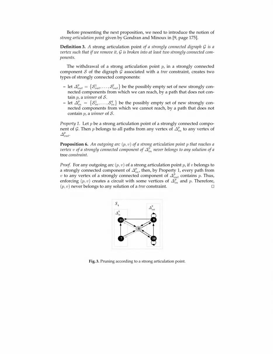
Fig. 3. Pruning according to a strong articulation point.

Example 4. Figure 3 illustrates Proposition 6 on the strongly connected compo-nent S4 of the digraph G depicted by part (A) of Figure 1. Vertex 8 is a strongarticulation point since its removal breaks S4 into four strongly connected com-ponents. 9 and 10 are potential root vertices, and since 7 and 11 have neitherloops nor connecting arcs, we have ∆8

out = {{9}, {10}} and ∆8

in = {{7}, {11}}.Then, from Proposition 6, the arcs (8, 7) and (8, 11) (drawn in gray in Figure 3)are infeasible.

We now introduce a final proposition that allows us to prune according tothe fact that we have to build a vertex-disjoint partitioning compatible withdom(NTREE).

Proposition 7. Let C = dom(NTREE) ∩ [MINTREE, MAXTREE]. For each strongly con-nected component S of G:

1. If S is a sink component of G that contains one single potential root r, then all theoutgoing arcs of r, except the loop (r, r), are infeasible.

2. Otherwise:2.1. If C = {MAXTREE} then, for each potential root r of S, all the non-loop arcs

(r, v) (v 6= r) are infeasible.2.2. If C = {MINTREE} and S is a non-sink component then all the loops of S are

infeasible.2.3. If there exists a single winner w in S, which is a door, then all the non-

connecting arcs (w, v) are infeasible.

Proof. For item 1, let r be the potential root of S and assume that we enforce anoutgoing arc (r, v) (v 6= r). Then, as S does not contain any doors, we cannotleave S and thus create a circuit involving at least two vertices. Item 2.1 (respec-tively 2.2) is a direct consequence of Proposition 2 (respectively Proposition 1).For item 2.3, assume that we have a single door w in S and consider that nopotential root belongs to S. If we do not take a connecting arc of w, then wecan never leave S and therefore we create a circuit in S involving at least twovertices. Thus, the tree constraint cannot hold. ut

Example 5. In order to illustrate Proposition 7 on the digraph depicted by part (A)of Figure 1, we consider the following three cases:

- First, we do not assume any restriction on dom(NTREE). Then, in this con-text, item 1 removes the arc (6, 5), while item 2.3 removes (1, 2).

- If NTREE is equal to MAXTREE (i.e., 4) then, in addition to the arcs removedby items 1 and 2.3, item 2.1 removes the arcs (4, 3), (9, 8), (9, 11), (10, 8) and(10, 9) since a loop is enforced for each of the vertices 4, 9 and 10.

- If NTREE is equal to MINTREE (i.e., 2) then, in addition to the arcs removed byitems 1 and 2.3, item 2.2 removes the arc (4, 4).

3.2 Arc-consistency

Now, we prove that Propositions 5, 6 and 7 characterise all the arcs that do notbelong to any solution of a tree constraint. For this purpose, we assume that thenecessary and sufficient condition of Proposition 3 holds.

Proposition 8. If Proposition 3 holds then the two following equivalences lead to thecompleteness of the pruning rules:

- Let t ∈ dom(NTREE), then t is incompatible with a tree constraint if and only if tis pruned by Proposition 5.

- Let (u, v) ∈ E , then (u, v) is incompatible with a tree constraint if and only if(u, v) is removed by at least one proposition among Propositions 6 and 7.

Proof. We first prove that Proposition 5 removes all infeasible values in the do-main of NTREE. Indeed, we have completeness since Proposition 3 enforces foreach t ∈ [MINTREE, MAXTREE] the existence of a vertex-disjoint partitioning of Gwith t trees.

Second, we prove that Propositions 6 and 7 remove all infeasible values forthe father variables. Now, for each arc (u, v) that was not pruned by Propo-sitions 6 or 7, we show how to build a vertex-disjoint partitioning of G with ttrees, where t ∈ dom(NTREE) ∩ [MINTREE, MAXTREE].

STEP 1Let dom(NTREE) ∩ [MINTREE, MAXTREE] = [mintree, maxtree],A1 Selecting a root in each sink component of G:

For each sink component S of G, if u is a potential root of S and u = vthen (u, v) has to be enforced. Otherwise, we select a potential root r ofS different from u and we enforce the loop (r, r). Observe that item 1 ofProposition 7 garanties us to find a potential root different from u. LetR1 denote the set of thus selected roots in the different sink componentsof G.

A2 Completing the set of roots in order to get mintree or mintree + 1trees:

CASE 1: mintree > MINTREE

Since we have to build at least mintree trees, we choose to buildexactly mintree trees. Therefore, we enforce a set R2 of mintree−MINTREE potential roots distinct from R1. Observe that if u = v andu does not belong to any sink component then u must belong toR2.CASE 2: mintree = MINTREE

• If u = v and u does not belong to any sink component thenMINTREE < MAXTREE and we have to enforce the loop (u, u), andR2 = {u}. Therefore, we choose to build mintree+ 1 trees.

• Otherwise, we build mintree trees andR2 = ∅.A3 Selecting a door in the strongly connected components that do not

contain a vertex of R1 ∪ R2.For all the strongly connected components S = (VS , ES) for which noloops are enforced (i.e., VS ∩ (R1 ∪ R2) = ∅):

• If u ∈ VS and (u, v) is a connecting arc, then (u, v) is enforced. Ob-serve that if u is the only door of S then v /∈ VS by item 2.3 ofProposition 7.

• Otherwise, if u, v ∈ VS or u /∈ VS then a door w, different from u, ischosen and we enforce one of its connecting arcs.

Let R3 denote the set of thus selected doors.STEP 2For a given strongly connected component S = (VS , ES):

- Let HS = VS ∩ (R1 ∪ R2 ∪ R3).- Let LS = VS −HS .- Let AS = {(u, v)} if u, v ∈ VS , otherwise AS = ∅.

For each strongly connected component S of G, we call the function intro-duced in Lemma 1 (see the Appendix), TreeCovering(S,HS ,LS ,AS), in or-der to build a vertex-disjoint partitioning of S with |HS | trees that includes(u, v) if u, v ∈ VS .

Thus, for each arc (u, v) ∈ E that is not pruned by Propositions 6 or 7, wehave shown how to build a vertex-disjoint partitioning of G with t trees, wheret ∈ dom(NTREE) ∩ [MINTREE, MAXTREE]. ut

3.3 Polynomial Arc-Consistency Algorithm

We show how to process all the pruning rules inO(n·m) time. Two parts are dis-tinguished, the first one only considers the pruning according to the strong ar-ticulation points (Proposition 6), the second one considers the pruning of NTREE(Proposition 5) and the pruning related to Proposition 7.

Then, in the first part, we are interested in Proposition 6 and we proposethe TreeFiltering algorithm below. For this purpose we have to detect all thestrong articulation points of a strongly connected component of G:

- Finding the strong articulation points takes at the maximum O(n ·m) timebecause we have not found a more efficient algorithm than withdrawing avertex and testing if the remaining subgraph is strongly connected or not.

- Detecting the arcs to be pruned takes O(n · m) time because for each ofthe strongly connected components S we have to withdraw each strongarticulation point p detected:• we have to search ∆p

in, thanks to a depth-first search beginning fromthe winners of S.

• we mark the vertices reachable from at least one winner as vertices of∆p

out.• we remove the arcs, that reach ∆p

in vertices from p, according to Propo-sition 6.

Now, in the second part, it is straightforward that the pruning related toProposition 5 is carried out in constant time. Moreover, the pruning related tothe general Proposition 7 consists of four steps:

- Items 1 and 2.3 of Proposition 7: the time complexity of these steps lies inthe construction of the reduced digraph, which takes O(m + n) time.

- Item 2.1 of Proposition 7: all the potential roots have to be detected, thattakes O(n) time.

- Item 2.2 of Proposition 7: we have to detect all the non-sink components ofG; then the time complexity lies in the construction of the depth-first searchin O(n + m) time.

TreeFiltering(G) : R.Input : the digraph G.Output :R the set of prunable arcs of G.R← ∅; \\ the set of arcs pruned.W ← {u |u is a winner};For each vertex scc of G doΨscc ← ∅; \\ the set of the strong articuation points of scc.\\ we detect the strong articulation points (s.a.p.) of scc.For each vertex u of scc do

if scc without u is not strongly connected then Ψscc ← Ψscc ∪ {u};\\ we search infeasible arcs.For each vertex u of Ψscc do PruneArcs(u, scc, W,R);

PruneArcs(u, scc, W,R) : RInput : a strongly connected component scc, a strong articulation pointu of scc, the set W of winners and the setR.Output :R the set of prunable arcs, increased by those discovered in scc.For each vertex v of scc do reach[v]← false;\\ detecting the blocks obtained by the withdrawal of each s.a.p. of scc.Σu

scc ← {Cu

1 , ..., Cu

m};\\ we search in each block the infeasible arcs.For each Cu

i ∈ Σu

scc dosearch[Cu

i ]← false;For each w ∈ W such that (w ∈ Cu

i ∧ ¬reach[w]) ∨ (w = u ∧ ¬search[Cu

i ]) doVisit(w, u, reach[ ]);

search[Cu

i ]← true;\\ withdrawal of infeasible outgoing arcs of u.If ∃(u, v) ∈ E such that v ∈ Cu

i ∧ ¬reach[v] thenW ← W ∪ {u};R ← R∪ {(u, v)};

Visit(v, u, reach[ ]) : reach[ ]Input : a winner v, a strong articulation point u and a boolean table reach[ ].Output : the table reach[ ].reach[v]← true;For each v 6= u and w ∈ pred[v] such that ¬reach[w] do Visit(w, u, reach[ ]);

TreeFiltering algorithm

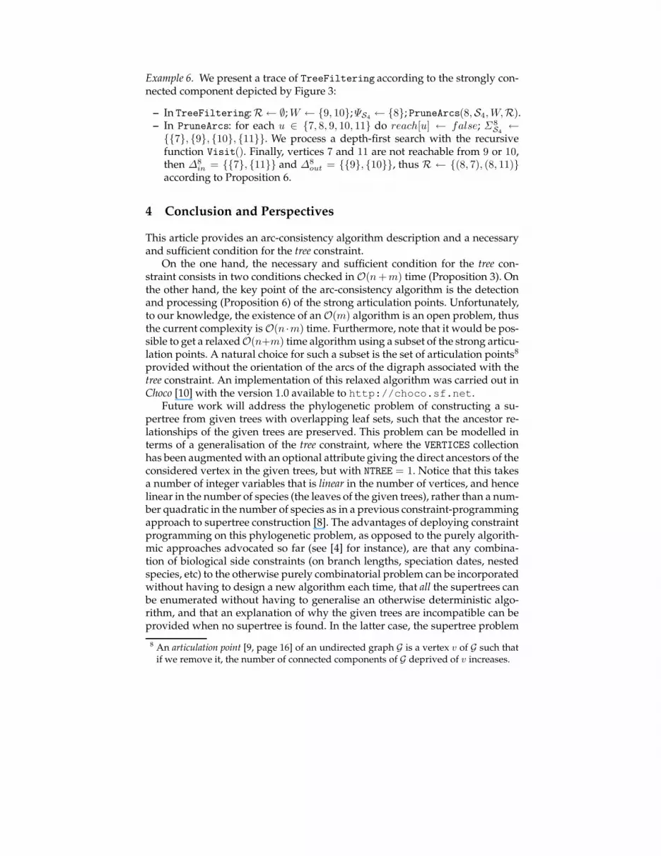
Example 6. We present a trace of TreeFiltering according to the strongly con-nected component depicted by Figure 3:

– In TreeFiltering:R ← ∅; W ← {9, 10}; ΨS4← {8}; PruneArcs(8,S4, W,R).

– In PruneArcs: for each u ∈ {7, 8, 9, 10, 11} do reach[u] ← false; Σ8

S4←

{{7}, {9}, {10}, {11}}. We process a depth-first search with the recursivefunction Visit(). Finally, vertices 7 and 11 are not reachable from 9 or 10,then ∆8

in = {{7}, {11}} and ∆8

out = {{9}, {10}}, thus R ← {(8, 7), (8, 11)}according to Proposition 6.

4 Conclusion and Perspectives

This article provides an arc-consistency algorithm description and a necessaryand sufficient condition for the tree constraint.

On the one hand, the necessary and sufficient condition for the tree con-straint consists in two conditions checked in O(n + m) time (Proposition 3). Onthe other hand, the key point of the arc-consistency algorithm is the detectionand processing (Proposition 6) of the strong articulation points. Unfortunately,to our knowledge, the existence of anO(m) algorithm is an open problem, thusthe current complexity isO(n ·m) time. Furthermore, note that it would be pos-sible to get a relaxedO(n+m) time algorithm using a subset of the strong articu-lation points. A natural choice for such a subset is the set of articulation points8

provided without the orientation of the arcs of the digraph associated with thetree constraint. An implementation of this relaxed algorithm was carried out inChoco [10] with the version 1.0 available to http://choco.sf.net.

Future work will address the phylogenetic problem of constructing a su-pertree from given trees with overlapping leaf sets, such that the ancestor re-lationships of the given trees are preserved. This problem can be modelled interms of a generalisation of the tree constraint, where the VERTICES collectionhas been augmented with an optional attribute giving the direct ancestors of theconsidered vertex in the given trees, but with NTREE = 1. Notice that this takesa number of integer variables that is linear in the number of vertices, and hencelinear in the number of species (the leaves of the given trees), rather than a num-ber quadratic in the number of species as in a previous constraint-programmingapproach to supertree construction [8]. The advantages of deploying constraintprogramming on this phylogenetic problem, as opposed to the purely algorith-mic approaches advocated so far (see [4] for instance), are that any combina-tion of biological side constraints (on branch lengths, speciation dates, nestedspecies, etc) to the otherwise purely combinatorial problem can be incorporatedwithout having to design a new algorithm each time, that all the supertrees canbe enumerated without having to generalise an otherwise deterministic algo-rithm, and that an explanation of why the given trees are incompatible can beprovided when no supertree is found. In the latter case, the supertree problem

8 An articulation point [9, page 16] of an undirected graph G is a vertex v of G such thatif we remove it, the number of connected components of G deprived of v increases.

can also be re-cast as an optimisation problem, and constraint programmingwill facilitate experiments with emerging cost functions.

Acknowledgements. This project was partially funded by grant HPRI-CT-2001-00153 within the Human Research Potential and Socio-Economic Knowledge Base:Access to Research Infrastructures (ARI) programme of the European Commis-sion, when the first author visited the second author at The Linnaeus Centre forBioinformatics. Finally, the implementation of the constraint would not havebeen possible without the relevant advice of Hadrien Cambazard and Guil-laume Rochart regarding JChoco.

References

1. E. Althaus, D. Duchier, A. Koller, K. Mehlhorn, J. Niehren, and S. Thiel. An effi-cient graph algorithm for dominance constraints. Journal of Algorithms, 48(1):194–219, May 2003. Special Issue of SODA 2001.

2. N. Beldiceanu. Global constraints as graph properties on structured network ofelementary constraints of the same type. Technical report, SICS T2000:01, Sweden,January 2000.

3. N. Beldiceanu and E. Contejean. Introducing global constraint in CHIP. Mathl.Comput. Modelling, 20(12):97–123, 1994.

4. O. R. Bininda-Emonds, editor. Phylogenetic Supertrees: Combining Information to Revealthe Tree of Life. Kluwer, 2004.

5. H. Cambazard and E. Bourreau. Conception d’une contrainte globale de chemin.JNPC, pages 107–120, 2004. In French.

6. Z.-Z. Chen. Efficient algorithms for acyclic colorings of graphs. Theoretical ComputerScience, 230(1-2):75–95, 2000.

7. M. Dincbas, P. V. Hentenryck, H. Simonis, T. G. A. Aggoun, and F. Berthier. TheConstraint Logic Programming Language CHIP. In Int. Conf. on Fifth GenerationComputer Systems (FGCS’88), pages 693–702, Tokyo, Japan, 1988.

8. I. P. Gent, P. Prosser, B. M. Smith, and W. Wei. Supertree construction using con-straint programming. In F. Rossi, editor, Proceedings of CP’03, volume 2833 of LNCS,pages 837–841. Springer-Verlag, 2003.

9. M. Gondran and M. Minoux. Graphes et algorithmes. Eyrolles, Paris, 2nd edition,1985. In French.

10. F. Laburthe and the OCRE group. CHOCO: implementing a CP kernel. In CP00 PostConference Workshop on Techniques for Implementing Constraint programming Systems(TRICS), Singapore, Sept. 2000.

11. J.-L. Laurière. A language and a program for stating and solving combinatorialproblems. Artificial Intelligence, 10:29–127, 1978.

12. J.-F. Puget. A C++ Implementation of CLP. In Second Singapore International Confer-ence on Intelligent Systems (SPICIS), pages 256–261, Singapore, November 1994.

13. A. Roychoudhury and S. Sur-Kolay. Efficient algorithms for vertex arboricity of pla-nar graphs. In Proceedings of the 15th Conference on Foundations of Software Technologyand Theoretical Computer Science, volume 1026 of LNCS, pages 37–51. Springer-Verlag,1995.

14. M. Sellmann. Reduction techniques in Constraint Programming and Combinatorial Opti-mization. PhD thesis, University of Paderborn, 2002.

15. M. Sellmann. Cost-based filtering for shortest path constraints. In 9th internationalConference on the Principles and Practice of Constraint Programming (CP), volume 2833of LNCS, pages 694–708. Springer-Verlag, 2003.

16. R. Tarjan. Depth-first search and linear graph algorithms. In SIAM J. Comput., vol-ume 1, pages 146–160, 1972.

Appendix

Lemma 1 is used in the proofs of Propositions 3 and 8. It presents a constructivemethod for building a vertex-disjoint partitioning into anti-arborescences of aparticular digraph depicted by the assumptions 1, 2 and 3.

Lemma 1. Let G = (V , E) be a digraph such that:

(1) Let H,L ⊆ V such thatH ∪ L = V andH ∩ L = ∅.(2) For each v ∈ L there exists a path from v to at least one vertex of H.(3) Let A ⊂ E such that |A| ≤ 1 and if |A| = 1 then A = {(u, v)}.

The following algorithm computes |H| vertex-disjoint anti-arborescences and havingtheir roots in H:

TreeCovering(G,H,L,A) : FInput : G,H,L,A.Output : F , the set of vertex-disjoint anti-arborescences.

F ← ∅;While L 6= ∅ doIf A 6= ∅ and ∃h ∈ H such that (v, h) ∈ E thenF ← F ∪ {(v, h), (u, v)};H ← H ∪ {u, v};L ← L− {u, v};

ElseLet w ∈ L and h ∈ H such that (w, h) ∈ E ;F ← F ∪ {(w, h)};H ← H ∪ {w};L ← L− {w};

Proof. By assumption (2), we know that from every vertex w ∈ L there existsa path to at least one vertex of H. Thus we make sure that L will become anempty set, i.e., that all vertices of V are covered. ut