Import elasticities and the external constraint in Mexico

Import elasticities and the external constraint in Mexico

Carlos A. Ibarra *

Department of Economics, Universidad de las Americas Puebla, Santa Catarina Martir s/n, Cholula, Pue. 72820, Mexico

1. Introduction

During the 1980s the Mexican government changed its economic strategy dramatically, in part byliberalizing the country’s trade regime and founding growth on the expansion of manufactured exports.The new strategy yielded mixed results. Trade flows grew rapidly: the average of exports and importsrose from 10% to 40% of GDP, while manufactures grew from 30% to 80% of exports. But despite the rapidexpansion of trade, GDP growth averaged a tepid 3.1% during the 1988–2006 post-liberalization period.

Economic Systems 35 (2011) 363–377

A R T I C L E I N F O

Article history:

Received 19 April 2010

Received in revised form 6 September 2010

Accepted 7 September 2010

Available online 2 April 2011

JEL classification:

F14

F43

O11

O19

O54

Keywords:

Import elasticities

External constraint

ARDL bounds testing approach

VECM model

Maquila

Vertical specialization

Mexico

A B S T R A C T

The paper estimates and analyzes an equation for intermediate

imports in Mexico during the 1988–2006 post-liberalization period.

While some results are obtained from Johansen’s VECM model, most

of the analysis is carried out within an Error-Correction ARDL

framework, following the bounds testing approach of Pesaran et al.

(2001). Besides showing that an aggregate equation for intermediate

imports can be satisfactorily estimated, the paper focuses on two

specific results. First, exports have a very significant effect on

imports, and failure to control for this effect (as in most previous

studies) can yield misleading results, like an over-estimation of the

output elasticity of imports. Second, the response of imports to

variations in the real exchange rate has fallen over time, presumably

because of the rising share of maquila in Mexico’s export basket and

the increasing ‘‘vertical specialization’’ of non-maquila export

production. Some implications of the estimation results are briefly

discussed, making reference to the possible external constraint on

Mexico’s economic growth.

� 2011 Elsevier B.V. All rights reserved.

* Tel.: +52 222 2292469.

E-mail address: [email protected].

Contents lists available at ScienceDirect

Economic Systems

journal homepage: www.elsevier.com/locate/ecosys

0939-3625/$ – see front matter � 2011 Elsevier B.V. All rights reserved.

doi:10.1016/j.ecosys.2010.09.004

http://dx.doi.org/10.1016/j.ecosys.2010.09.004

mailto:[email protected]

http://www.sciencedirect.com/science/journal/09393625

http://dx.doi.org/10.1016/j.ecosys.2010.09.004

There is wide disagreement about the role of trade liberalization in Mexico’s puzzling blend oftrade success and growth failure. Some analysts argue that liberalization has not gone far enough:further liberalization would give local firms better access to foreign production goods, increase thefirms’ productivity, and result in stronger export and GDP growth (see Moissinac, 2006; Haugh et al.,2008; OECD, 2005; WTO, 2008a,b).

Others argue that liberalization went too far and led to an excessive penetration of imports, assuggested by an increase in the output elasticity of imports and/or in the ratio of the trade deficit to theGDP growth rate. The consequence would be a tightening of the external constraint on economicgrowth, that is, a fall in the GDP growth rate consistent with a trade balance target (see Moreno-Brid,1999; Lopez and Cruz, 2000; Ocegueda, 2000; Guerrero de Lizardi, 2003; Ibarra, 2003; Cardero andGalindo, 2005; Pacheco-Lopez, 2005; Moreno-Brid et al., 2005; Pacheco-Lopez and Thirlwall, 2007;Moreno-Brid and Ros, 2009, chapter 8).

The present paper contributes to this literature by estimating and analyzing an equation forintermediate imports in Mexico during the 1988–2006 post-liberalization period.1 The importequation is derived from several Error-Correction Autoregressive Distributed Lag (EC-ARDL)models, following the bounds testing approach of Pesaran et al. (2001). Where allowed by thedata, the results are compared with those obtained from Johansen’s Vector Error Correction model(VECM).

Besides showing that an aggregate equation for intermediate imports can be satisfactorilyestimated, the paper presents two other main results. First, it shows the importance of includingexports as a separate determinant of the demand for intermediate imports in Mexico. Failing to doso (as in most previous studies) can yield misleading results, like an over-estimation of the outputelasticity of imports and an under-estimation of the real exchange rate elasticity.

Second, the paper presents strong evidence of a gradual fall in the response of imports to variationsin the real exchange rate, a result to be expected from both the rising share of maquila (in-bondproduction) in Mexico’s export basket and the increasing ‘‘vertical specialization’’ of non-maquilaexport production.2 Because of the declining response of imports, the real exchange rate may becomeless effective to offset the before-mentioned increase in the trade deficit ratio, with negativeconsequences for Mexico’s growth perspectives.

The paper is organized as follows. Section 2 describes the data and econometric methodology.Section 3 presents the general estimation results. Section 4 takes a closer look at the determination ofthe import elasticities and briefly discusses some implications for economic growth in Mexico, makingreference to the possible role of the external constraint. Section 5 presents the conclusions.Appendix A details data sources and definitions.

2. Data and methodology

We explore the existence of long-run, or level, effects on imports of intermediate goods inMexico. Our theoretical framework is the imperfect substitutes model, where the demand forimports is assumed to depend on domestic output and the relative price between foreign anddomestic goods (for example, see Chinn, 2006; Bayoumi, 1999, and the references therein). Thisframework has been widely used to study the determination of foreign trade flows in Mexico (forexample, see Bahmani-Oskooee and Hegerty, 2009; Pacheco-Lopez, 2005; Fullerton and Sprinkle,2005; McDaniel and Agama, 2003).3 To test one of our main hypotheses, to this basic frameworkwe add exports as a possible determinant of intermediate imports.

1 Intermediate goods are the largest component of Mexico’s imports, with a share of about 60% before the enactment of

NAFTA in 1994, and close to 70% afterwards.2 ‘‘Vertical specialization’’ is understood here as the import of intermediate goods by multinational corporations for assembly

and export; see Feenstra (1998) and Hummels et al. (2001) for international evidence, and Cardero and Galindo (2005) and

Ibarra (2010a) for the Mexican case.3 For recent applications to other countries and regions, see Bahmani-Oskooee and Ratha (2008), Irandoust et al. (2006), and

Sissoko and Dibooglu (2006).

C.A. Ibarra / Economic Systems 35 (2011) 363–377364

The presumed long-run equation for intermediate imports is:

INTLR ¼ a þ eEXP þ pIPI þ rREER (1)

where INTLR is the long-run level of real intermediate imports, EXP real non-oil exports, IPI theindustrial production index, and REER the consumer price-based real effective exchange rate, where arise indicates a real peso depreciation. Depending on the specific equation to be estimated, trade datamay or may not include maquila. Since the variables are measured in natural logarithms, thecoefficients in Eq. (1) represent import elasticities (see Appendix A for data sources and definitions).

Eq. (1) will be estimated according to the bounds testing approach of Pesaran et al. (2001). Thereare two main steps. In the first one, the following Error-Correction Autoregressive Distributed Lag (EC-ARDL) model is estimated:

DINTt ¼ g0 þ sINTt�1 þX3

i¼1

g iZi;t�1 þXm

j¼1

d jDINTt� j þX3

i¼1

Xm

j¼0

bi; jDZi;t� j (2)

where the Z variables are exports, the industrial production index, and the real exchange rate. Whilethe number of lags m is conventionally determined by the Akaike information criterion, the statisticaladequacy of the estimated equation must be confirmed by a battery of diagnostic tests before movingon to the next step.

In the second step, bounds testing is carried out to establish the existence of cointegration (seebelow). Once cointegration has been established, the long-run coefficients in Eq. (1) can be retrievedfrom the estimated coefficients in Eq. (2) as �gi/s for each regressor i. After the long-run coefficientshave been obtained, the existence of cointegration can be further confirmed, a la Engle–Granger, byrejecting the hypothesis of a unit root in the long-run error, INT� INTLR, where INT is the observed levelof intermediate imports, and, as mentioned, INTLR is the long-run level calculated with the estimatedcoefficients from Eq. (1).

There are two bounds tests of cointegration. First, s in Eq. (2), which would correspond to thecoefficient on the lagged long-run error in a standard error-correction model, must be negative,indicating that the dependent variable moves over time toward its long-run equilibrium at speed s.Pesaran et al. (2001) provide lower and upper critical values for the t-test, depending on whether thevariables are integrated of order zero (lower bound) or one (upper bound). Cointegration isunambiguously accepted when, in absolute value, the t-statistic lies above the upper critical bound.

The second is an F-test for the significance of the level coefficients, under the null that s and the g’sin Eq. (2) are jointly equal to zero. Again, Pesaran et al. (2001) provide lower and upper critical valuesthat depend on order of integration. Cointegration is unambiguously accepted when the F-statistic liesabove the upper bound. Since the Pesaran et al. critical values are valid only asymptotically, therelevant tables in the next sections also report the small-sample critical values for the F-test computedby Narayan (2005).

The bounds testing approach has several advantages. First, compared with multiple-equationmethodologies, it has good small-sample properties—a key advantage given the limited number ofobservations in some of our regressions. Second, in contrast to other methodologies, it can combine inthe same equation variables that are integrated of order zero or one—although not higher. Finally, aswe have seen, it estimates in a single stage both the long- and short-run coefficients, including that onthe long-run error.

Although not much discussed in applications of the bounds testing approach, a further advantageof ARDL models in general is that they yield unbiased estimates of the long-run coefficients even ifsome of the regressors are endogenous (see Harris and Sollis, 2003, chap. 4). In any event, as arobustness check, and where allowed by the data, some results will be obtained from Johansen’sVector Error Correction (VECM) model (see Juselius, 2006). Since it estimates a system of equations byMaximum Likelihood, the VECM model alleviates the potential problem of endogeneity among theregressors. Also, it tests for the existence of, and simultaneously estimates, multiple cointegrationrelationships. The model, however, requires the estimation of a large number of coefficients, which isproblematic given our relatively small sample period. This would make it practically impossible tocarry out some of the main exercises presented in the paper.

C.A. Ibarra / Economic Systems 35 (2011) 363–377 365

The benchmark estimation period runs from 1988 to 2006. The period begins after completion ofthe first stage of trade liberalization, which took place from 1985 to 1987 (see Ros, 1994; Sanchez et al.,1994), and ends on the date the Mexican government stopped reporting separate data for maquila andnon-maquila trade flows. In the estimations that use the relative labor cost in the manufactures as analternative measure of the real exchange rate, the sample begins in 1993 due to limited dataavailability. All the series are monthly, except in the VECM estimations, which use quarterly series toimprove the diagnostics.

3. General results

We begin with the VECM results. The endogenous variables in the underlying vectorautoregression (VAR) model are non-maquila exports and imports and the industrial productionindex. The exogenous variables are the real exchange rate (since the model lacks the asset-marketvariables and other ‘‘fundamentals’’ needed for a meaningful analysis of exchange rate determina-tion4) and the U.S. industrial production index (under the assumption that the Mexican economy is toosmall to affect U.S. production levels). While not reported in the tables, all the models in the paperinclude a constant.

To account for possible seasonal effects, given the use of quarterly series, the variables are enteredwith four lags. The VAR passes the system tests for normality and heteroscedasticity, but cannot passthe test for serial correlation. The problem persists even if one lag is either added or subtracted, whilethe normality test then fails. Single-equation tests (available upon request) reveal that the source ofthe problem lies in the VAR import equation. While the VECM results must thus be taken with somecaution, the coefficient estimates are qualitatively similar to those obtained in the EC-ARDL model,which does pass all the diagnostic tests.

The number of cointegration relationships can be determined by the so-called trace test. The tracestatistic was corrected for small-sample bias as suggested by Johansen (2002), while the test’s criticalvalues were taken from Pesaran et al. (2000), who control for the number of exogenous variables. Thetrace test indicates the existence of two cointegration relationships. According to the sign and size ofthe coefficients, and supported by the results of the likelihood ratio (LR) test of restrictions, thoserelationships can be interpreted as long-run equations for imports and industrial production (seeTable 1).

While not the focus of the paper, we can briefly describe the second cointegration equation. Itshows that the pace of Mexico’s industrial production follows that of the U.S. closely (with a highelasticity of 0.91), but with a significant effect from the real exchange rate (with an elasticity of 0.18).Thus, a currency depreciation accelerates Mexico’s relative industrial growth, at least during atransition period.5

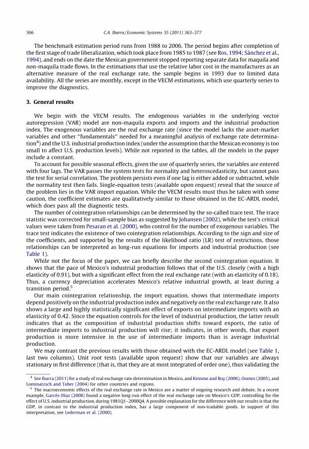
Our main cointegration relationship, the import equation, shows that intermediate importsdepend positively on the industrial production index and negatively on the real exchange rate. It alsoshows a large and highly statistically significant effect of exports on intermediate imports with anelasticity of 0.42. Since the equation controls for the level of industrial production, the latter resultindicates that as the composition of industrial production shifts toward exports, the ratio ofintermediate imports to industrial production will rise; it indicates, in other words, that exportproduction is more intensive in the use of intermediate imports than is average industrialproduction.

We may contrast the previous results with those obtained with the EC-ARDL model (see Table 1,last two columns). Unit root tests (available upon request) show that our variables are alwaysstationary in first difference (that is, that they are at most integrated of order one), thus validating the

4 See Ibarra (2011) for a study of real exchange rate determination in Mexico, and Kemme and Roy (2006), Oomes (2005), and

Lommatzsch and Tober (2004) for other countries and regions.5 The macroeconomic effects of the real exchange rate in Mexico are a matter of ongoing research and debate. In a recent

example, Garces-Dıaz (2008) found a negative long-run effect of the real exchange rate on Mexico’s GDP, controlling for the

effect of U.S. industrial production, during 1981Q1–2000Q4. A possible explanation for the difference with our results is that the

GDP, in contrast to the industrial production index, has a large component of non-tradable goods. In support of this

interpretation, see Lederman et al. (2000).


bounds testing approach. According to the Akaike criterion and the diagnostics results, the modelincludes three lags in the first-differenced variables. Cointegration is amply accepted by the twobounds tests, while the hypothesis of a unit root in the long-run error is rejected. The new long-runcoefficients are similar to the VECM estimates. Intermediate imports depend positively on industrialproduction and exports, with elasticities of 1.23 and 0.4, respectively, while they depend negatively onthe real exchange rate, with an elasticity of 0.25.

The results indicate that, even under conditions of a tight link between exports and imports,variations in the real exchange rate can alter Mexico’s trade balance (in U.S. dollars). To confirm that theconclusion does not depend on our specific measure of the real exchange rate, the import equation wasre-estimated, but using, as an alternative measure, the ratio of the unit labor cost in the manufacturesbetween the U.S. and Mexico (RULC). Because of the limited availability of the RULC series, the estimationsample was shortened to June 1993–December 2006. The Akaike criterion and model diagnostics again

Table 1Import cointegration equations (ex maquila).

VECM EC-ARDL I EC-ARDL II

Dependent variable Intermediate

imports, INT

Industrial

production, IPI

Intermediate

imports, INT

Intermediate

imports, INT

Sample 1988Q1–2006Q4,

n=76

1988M1–2006M12,

n=228

1993M6–2006M12,

n=163

Long-run coefficients

Industrial production, IPI 1.083 (4.279) 1.231 (2.599) 1.227 (2.687)

Exports, EXP 0.423 (6.282) 0 0.396 (3.488) 0.371 (4.209)

Real exchange rate I, REER �0.204 (�1.978) 0.184 (2.805) �0.249 (�1.649)

Real exchange rate II, RULC �0.176 (�2.708)

U.S. industrial production 0 0.909 (14.45)

Long-run error, INT� INTLR �0.348 (�5.740) �0.049 (�3.427) �0.231 (�4.868) �0.446 (�4.388)

Unit-root tests on long-run error

ADF �5.255 [0.000] �2.986 [0.041] �5.476 [0.000] �4.645 [0.000]

Phillips-Perron �5.254 [0.000] �2.376 [0.152] �7.467 [0.000] �9.503 [0.000]

Diagnostics

Heteroscedasticity 0.940 [0.656]

Normality 9.524 [0.146] 0.617 [0.735] 0.166 [0.921]

Autocorrelation 2.728 [0.000] 0.724 [0.631] 1.187 [0.317]

ARCH 1.117 [0.292] 0.340 [0.560]

RESET 0.392 [0.532] 0.194 [0.660]

Trace test: H0: rank is equal to or less than

0 1 2

80.93 [46.44] 37.14 [28.42] 10.79 [14.35]

LR test of restrictions 1.849 (4) [0.764]

Bounds tests

F-test 6.295 [4.35] (4.52) 6.244 [4.35] (4.52)

t-test �4.868 [�3.78] �4.388 [�3.78]

Source: Author’s calculations.

(1) For illustrative purposes, t-statistics are shown in parenthesis next to the long-run coefficients. In the EC-ARDL models, the t-

statistics correspond to the gi coefficients from Eq. (2) (see main text). The industrial production equation in VECM includes a

zero restriction on the INT coefficient.

(2) The ADF (Augmented Dickey–Fuller) and Phillips–Perron tests include a constant and no trend. The number of lags in ADF

follows the Schwarz criterion (starting with a max of 12). P–P uses the Newey–West bandwidth. p-values in brackets.

(3) VECM diagnostics: Results shown for system (multiple-equation) tests. The null hypotheses are that there is no serial

correlation of up to fifth order, and that residuals are normally distributed and unconditionally homoscedastic.

(4) EC-ARDL diagnostics: The null hypotheses are that residuals are normally distributed (Jarque-Bera), that there is no serial

correlation of up to 6th order (Breusch–Godfrey) and no ARCH errors, and that the equation passes Ramsey’s mis-specification

test using the squares of the fitted values (RESET). x2 (Jarque-Bera) and F-statistics with p-values in brackets.

(5) The trace statistic was adjusted for small-sample bias according to Johansen (2002). 5% critical values in brackets from

Pesaran et al. (2000).

(6) The LR test shows, next to the x2-statistic, the number of restrictions in parenthesis and the p-value in brackets.

(7) Bounds tests show 5% asymptotic upper critical values from Pesaran et al. (2001) in brackets. The F-test shows small-sample

upper critical values from Narayan (2005), also at a significance level of 5% and for n=80 observations, in parenthesis.


suggested the inclusion of three lags in the first-differenced variables. Bounds testing supports theexistence of cointegration, which is confirmed by the stationarity of the long-run error.

While the estimated elasticities with respect to industrial production and exports are practicallyidentical to those obtained previously, the (absolute) value of the real exchange rate elasticity issmaller (0.18 rather than 0.25). There is the question, however, of whether the reduced real exchangerate coefficient reflects the alternative real exchange rate measure or the different estimation period.We will return to this issue in Section 4.2.2.

4. A closer look

4.1. The output elasticity of imports

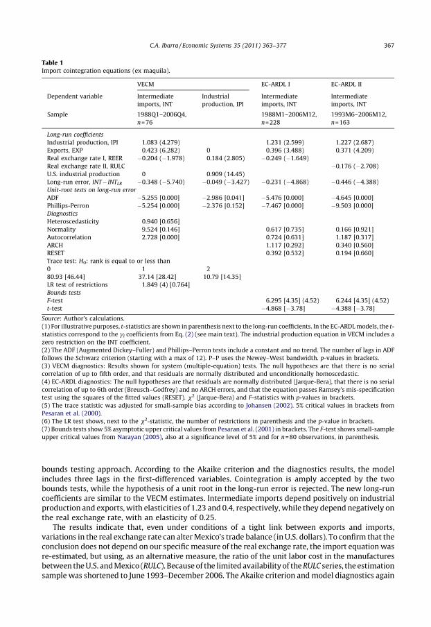
As noted in Section 1, many authors have looked for possible variations in the output elasticity ofimports to discuss the growth effects of trade liberalization in Mexico. Those studies, however, havenot controlled for the direct effect of exports on the demand for intermediate imports. How may theestimated elasticities of imports be affected by failing to control for this effect? Consider first theVECM results. There are several points to make (see Table 2). First, if the model is re-estimated with azero restriction on the export coefficient in the import equation, then the LR test rejects the model at1%. Thus, the model without exports in the import equation is mis-specified.

Second, the real exchange rate coefficient practically drops to zero. This unexpected result may beexplained by two opposite effects: by raising their cost in local currency, a real currency depreciationdirectly encourages a substitution of intermediate imports by local goods; at the same time, however,depreciation increases exports, and thus import demand. Not including exports in the import equationblurs the two effects and biases the exchange rate coefficient toward zero. Finally, if the exportcoefficient in the import equation is restricted to zero, then the industrial production coefficient morethan doubles from 1.08 to 2.37 (with a standard error of 0.14). Thus, failing to control for the direct

Table 2Import cointegration equations, excluding exports.

VECM EC-ARDL

Dependent variable Intermediate imports, INT Industrial production, IPI Intermediate imports, INT

Sample 1988Q1–2006Q4 1988M1–2006M12


Industrial production, IPI 2.368 (17.033) 2.677 (3.600)

Exports, EXP 0 0

Real exchange rate, REER �0.023 (�0.170) 2.237 (3.281) 0.214 (1.130)

U.S. industrial production 0 �0.823 (�1.260)

Long-run error, INT� INTLR �0.282 (�5.407) �0.004 (�2.600) �0.190 (�3.859)


EC-ARDL diagnostics

Normality Autocorrelation ARCH RESET

0.198 [0.906] 0.823 [0.553] 1.413 [0.236] 0.0282 [0.867]

Omitted-variable tests F-stat [prob]

Lagged export level, plus current and three lags of first difference 32.181 [0.000]

Lagged export level �5.096 [0.025]


(1) Trade data exclude maquila.

(2) For illustrative purposes, t-statistics are shown in parenthesis next to the long-run coefficients. In the EC-ARDL models, the t-

statistics correspond to the gi coefficients from Eq. (2) (see main text). The industrial production equation in VECM includes a

zero restriction on the INT coefficient.

(3) Diagnostics: The underlying VAR for the VECM is identical to that of Table 1, and thus presents the same diagnostic results.

For EC-ARDL, see explanation in Table 1.

(4) The LR test shows, next to the x2-statistic, the number of restrictions in parenthesis and the p-value in brackets.


effect of exports on imports introduces an upward bias in the estimation of the output elasticity ofimports.

Similar results are obtained in the EC-ARDL model: the real exchange rate coefficient shifts from�0.25, when exports are included in the import equation, to (positive) 0.21 when they are not, whilethe industrial production coefficient doubles from 1.23 to 2.68. Again, the new estimation resultsreflect a mis-specified model: an omitted-variable test amply rejects the hypothesis that exports canbe excluded from the estimation, whether the test considers exports only in levels or also in firstdifferences.

It may be wondered whether the export coefficient in the import equation is picking up not thedirect effect of export production on the demand for imports, but rather the balance of payments(BOP) restriction that forces export and imports to eventually follow a roughly similar trend. A firstthing to notice, though, is that our estimations have relied on specific components of trade flows(rather than their total amounts), which for that reason are less subject to the BOP restriction.

A second way to confirm our interpretation is by calculating the dynamic effect of exports onintermediate imports. While the BOP restriction is expected to hold over relatively long periods, in theshort run there can be significant fluctuations in the trade balance. If the link between exports andimports in our equations reflected the BOP restriction, then there should be no immediate response ofimports to export variations.

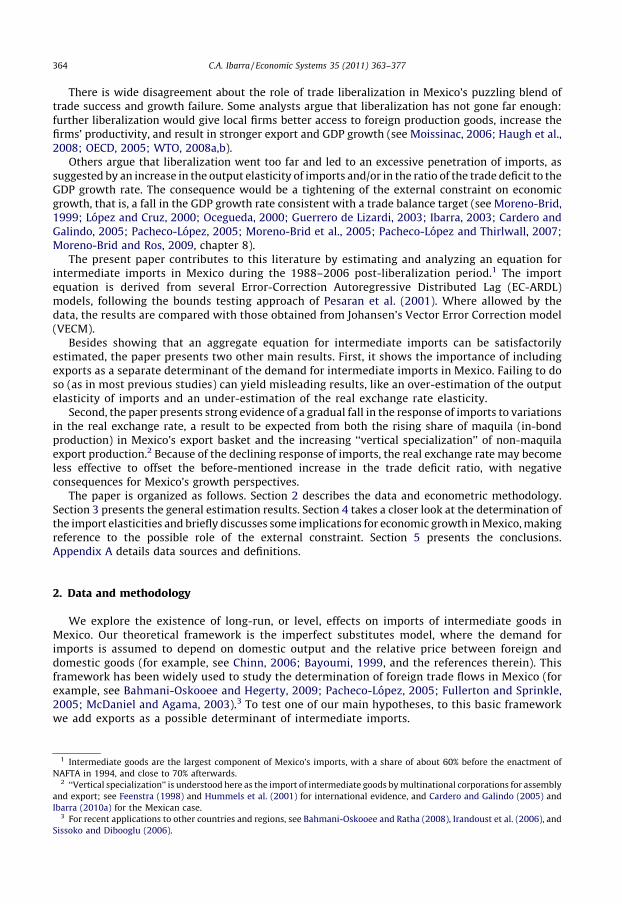
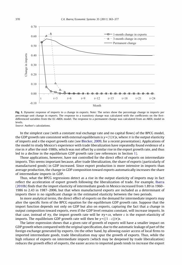
The dynamic response of imports can be calculated from the EC-ARDL import equation. Toconcentrate on the short-term response, we use the estimated coefficients on the first-differencedvariables (recall Eq. (2)). Since the variables are in logs, the calculated series represent the percentageresponse of imports to a transitory one percentage change in exports. We present two series, onewhere the export change is assumed to last for one month, and another where it lasts for three months.In the latter case, for example, we set DEXP=1 for t, t+1 and t+2, and zero otherwise. Recalling that theEC-ARDL was estimated with three lags for the variables in first differences, the response of imports iscalculated as:

DINTt ¼ b1;0DEXPt

. . .DINTtþ3 ¼ d1DINTtþ2 þ d2DINTtþ1 þ d3DINTt þ b1;1DEXPtþ2 þ b1;2DEXPtþ1 þ b1;3DEXPt

. . .DINTtþ5 ¼ d1DINTtþ4 þ d2DINTtþ3 þ d3DINTtþ2 þ b1;2DEXPtþ2; etc:

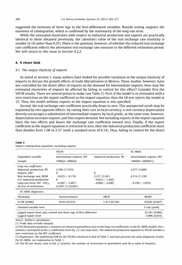
Fig. 1 shows the two series. In both we see that the import response fades out quickly, as should bethe case, given the transitory nature of the export change. It is more important, though, that importsrespond immediately. Since we are using monthly observations and the short-run coefficients fromthe first-differenced variables, such response must reflect the increased demand for intermediateimports by the export sector, rather than the longer-term BOP restriction.

A complementary view is provided by the dynamic response of imports to a permanent change inexports. For this exercise, the EC-ARDL model was re-estimated in its original, levels version. Since theerror correction model included three lags in the first-differenced variables, the ARDL model in levelshad to include four lags to ensure that the two specifications yielded identical long-run coefficients.

The estimated ARDL coefficients were used to simulate the response of imports to a permanent risein exports (see again Fig. 1). It takes about 18 months for the response to reach its ‘‘long-run’’ value of0.4, which was indeed the long-run export coefficient in the EC-ARDL equation. As can be seen,imports respond immediately to exports (in fact, overshooting their long-run response), reaching theirhighest value within the first three months. Again, given the use of monthly data, this very short-runresponse should be interpreted as picking up the direct effect of export production on import demand,rather than the longer-run BOP restriction.

The direct effect of exports on the demand for intermediate imports may have implications, bothempirical and analytical, for the study of the external constraint on economic growth. While itsbeyond the scope of this paper to give a full treatment of those implications, we may briefly considersome of them, using as framework the well-known balance-of-payments-constrained growth (BPCG)model.


In the simplest case (with a constant real exchange rate and no capital flows) of the BPCG model,the GDP growth rate consistent with external equilibrium is y=(1/p)x, where p is the output elasticityof imports and x the export growth rate (see Blecker, 2009, for a recent presentation). Applications ofthe model to study Mexico’s experience with trade liberalization have repeatedly found evidence of arise in p after the mid-1980s, which was not offset by a similar rise in the export growth rate, and thusled to a decline in the equilibrium GDP growth rate (see references in Section 1).

Those applications, however, have not controlled for the direct effect of exports on intermediateimports. This seems important because, after trade liberalization, the share of exports (particularly ofmanufactured goods) in GDP increased. Since export production is more intensive in imports thanaverage production, the change in GDP composition toward exports automatically increases the shareof intermediate imports in GDP.

Thus, what the BPCG regressions detect as a rise in the output elasticity of imports may in factreflect the acceleration of export growth following the liberalization of trade. For example, Ibarra(2010b) finds that the import elasticity of intermediate goods in Mexico increased from 1.89 in 1960–1986 to 2.43 in 1987–2006, but that when manufactured exports are included as a determinant ofimports there is no significant change in the estimated elasticity between the two periods.

In more analytical terms, the direct effect of exports on the demand for intermediate imports mayalter the specific form of the BPCG equation for the equilibrium GDP growth rate. Suppose that theimport function depends not only on GDP but also on exports, capturing the fact that a change inoutput composition toward exports, even if the GDP level remains constant, will increase imports. Inthat case, instead of py, the import growth rate will be py+ex, where e is the export-elasticity ofimports. The equilibrium GDP growth rate will then be y=((1�e)/p)x.

The latter expression shows that a given rate of growth of exports will have a smaller impact onGDP growth when compared with the original specification, due to the automatic leakage of part of theforeign exchange generated by exports. On the other hand, by allowing easier access of local firms toimported intermediate goods, trade liberalization may spur the growth of exports. Thus, while thehigh reliance of exports on intermediate imports (which may be deepened by trade liberalization)reduces the growth effect of exports, the easier access to imported goods tends to increase the export

-0.10

0.00

0.10

0.20

0.30

0.40

0.50

0.60

0.70

t t+3 t+6 t+9 t+ 12 t+ 15 t+ 18 t+ 21 t+ 24

Cha

nge

in im

ports

Month

1-month change in expo rts3-month change in expo rtsPermanent change

Fig. 1. Dynamic response of imports to a change in exports. Note: The series show the percentage change in imports per

percentage unit change in exports. The response to a transitory change was calculated with the coefficients on the first-

differenced variables from the EC-ARDL model. The response to a permanent change was calculated from an ARDL model in

levels.



growth rate. The net effect on growth is thus uncertain, and may depend on other variables like thereal exchange rate (see Ibarra, 2010a, for an initial analysis).

4.2. The real exchange rate elasticity

Several studies have reported a rise in the ratio of the trade deficit to the GDP growth rate in Mexicoin the post-liberalization period. The higher deficit may act as a constraint on the country’s rate ofeconomic growth: if the trade deficit is now higher for any given rate of GDP growth, then GDP growthmust fall to ensure that the deficit does not exceed a critical level. This conclusion remains valid even ifno change in import elasticities has taken place.

The rise in the trade deficit ratio underscores the important role that the real exchange rate mayplay in the macroeconomic adjustment to trade liberalization. The evidence presented in Section 3shows that a real depreciation of the peso reduces the gap between intermediate imports and exports.A more depreciated currency could offset the tightening of the external constraint caused by the rise inthe trade deficit ratio.

The future effectiveness of the real exchange rate to relax the constraint may be compromised,however, by two recent developments: the rising share of maquila goods in Mexico’s export basket,and the increasing ‘‘vertical specialization’’ of non-maquila export production, particularly after theenactment of NAFTA (see Ibarra, 2010a, for empirical evidence).6 Both developments imply anincreasingly close link between exports and intermediate imports that may not yield to variations inrelative prices.

Linking to our previous estimations, we may expect two results: first, for the entire post-liberalization period including maquila in trade flows should reduce the response of imports to thereal exchange rate and increase that to exports; and second, there should be a reduction over time inthe response of imports to the real exchange rate and an increase in that to exports, even if maquila isexcluded from trade flows.

4.2.1. The maquila effect

To explore the maquila effect, the import equation was re-estimated but adding maquila to importsand exports (see Table 3). In the VECM model, the trace test again indicates the existence of twocointegration relationships, which can be normalized in imports and industrial production. Asexpected, the export coefficient in the import equation is now notably larger, reflecting a tighter linkbetween exports and intermediate imports once they include maquila. At the same time, the realexchange rate coefficient not only loses significance but the LR test amply accepts that we drop thevariable from the import equation.

Turning to the EC-ARDL equation, the Akaike criterion and model diagnostics suggest the inclusionof five lags in the first-differenced variables. Cointegration is amply accepted by the bounds tests andthe stationarity of the long-run error. The new results are qualitatively similar to those obtained in theequation without maquila: imports depend negatively on the real exchange rate, and positively onexports and industrial production. But the quantitative results are quite different: the absolute valueof the estimated real exchange rate coefficient is now notably smaller (0.16 versus the original 0.25) asthe counterpart to a much larger export coefficient (0.65 versus 0.40). Similar results are obtainedwhen the equation includes RULC rather than REER.

4.2.2. Changing elasticities

Turning to the second prediction, a simple way to test for a change over time in import elasticities isto allow for different slope coefficients before and after the enactment of NAFTA (in our sample,January 1988–December 1993 and January 1994–December 2006).7 For that purpose, the EC-ARDL

6 According to BOP data in nominal U.S. dollars, maquila rose from 47% of manufactured exports in 1988 to 55% during 2000–

2006. The influence of vertical specialization on the response of imports to exchange rate variations has been much studied in

the Chinese case; see for example Cui and Syed (2007).7 Bahmani-Oskooee and Hegerty (2009), controlling for the real exchange rate, show that imports from the U.S. increased in

Mexico after the enactment of NAFTA, but do not explore whether there was a change in import elasticities.


import equation was re-estimated adding interactions between a NAFTA dummy and the laggedvariables in levels. Based on their individual significance, only the interactions with exports and thereal exchange rate were kept in the final equation. To facilitate interpretation, the initial estimationsexclude maquila (see Table 4).

The diagnostics remains amply satisfactory. The two bounds tests reject the null of zero levelcoefficients, while separate unit-root tests on the long-run error indicate the existence ofcointegration in both the pre-NAFTA and NAFTA periods. This specification yields one of theexpected results: there is a (dramatic) fall, from �0.45 to �0.07, in the absolute value of the realexchange rate coefficient in the NAFTA period. The result is consistent with the hypothesis that deepervertical specialization in non-maquila production is reducing the response of imports, once the effectof exports is controlled for, to variations in the real exchange rate.

While the previous exercise is attractive because of the significance of NAFTA for the Mexicaneconomy, it also has several disadvantages: one is the very different size (72 versus 156 observations)of the pre- and NAFTA sample periods; another, more serious, is that it forces a precise date ofstructural change, simultaneous for all coefficients, when in fact a more gradual and asynchronicchange may have taken place. Those disadvantages could account for the somewhat anomalous resultthat, while the estimated absolute value of the real exchange rate coefficient falls after the enactmentof NAFTA (as expected), the export coefficient also does so (which seems to contradict the hypothesisof deeper vertical specialization).

Thus, as a second exercise, separate EC-ARDL import equations were estimated for two non-overlapping samples: January 1988–December 1996 (108 observations) and January 1997–December2006 (120 observations) (see Table 3, last two columns). The new estimations confirm the dramaticchange in the real exchange rate coefficient from a very large (absolute) value of �0.44 in the early

Table 3Import cointegration equations (with maquila).

VECM EC-ARDL I EC-ARDL II

Dependent variable Intermediate

imports, INT

Industrial

production, IPI

Intermediate

imports, INT

Intermediate

imports, INT

Sample 1988Q1–2006Q4,

n=76

1988M1–2006M12,

n=228

1993M6–2006M12,

n=163


Industrial production, IPI 0.595 (3.265) 0.772 (2.345) 0.609 (1.808)

Exports, EXP 0.691 (14.605) 0 0.651 (4.379) 0.685 (4.182)

Real exchange rate I, REER 0 0.226 (3.647) �0.165 (�1.642)

Real exchange rate II, RULC �0.129 (�2.506)

U.S. industrial production 0 0.874 (14.732)



ADF �5.095 [0.000] �2.819 [0.060] �5.686 [0.000] �5.067 [0.000]

Phillips-Perron �5.095 [0.000] �2.336 [0.164] �7.682 [0.000] �8.387 [0.000]

Diagnostics

Heteroscedasticity 0.976 [0.562]

Normality 4.714 [0.581] 2.430 [0.297] 1.346 [0.510]

Autocorrelation 2.992 [0.000] 0.948 [0.462] 0.640 [0.698]

ARCH 0.097 [0.756] 1.936 [0.166]

RESET 1.374 [0.243] 1.994 [0.160]

Trace test: H0: rank is equal to or less than

0 1 2

76.13 [46.44] 36.38 [28.42] 9.70 [14.35]


Bounds tests

F-test 6.178 [4.35] (4.52) 4.400 [4.35] (4.52)

t-test �4.903 [�3.78] �3.828 [�3.78]


Notes: see Table 1.


sample to 0.04 in the late one; moreover, while only suggestive given the use of non-stationary data,the coefficient’s t-statistic falls from 2.24 to 0.5.

The changes in the other cointegration coefficients are now consistent with the hypothesis ofdeeper vertical specialization: while the elasticity of imports with respect to the industrial productionindex fell from 1.42 to 0.68 (and became less statistically significant), that with respect to exports rosefrom 0.47 to 0.92.

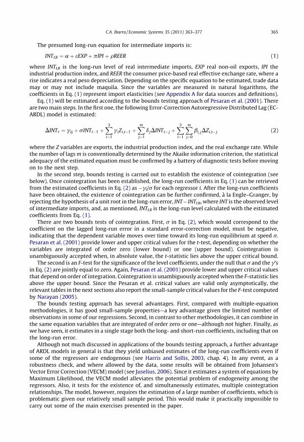
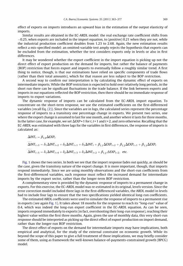
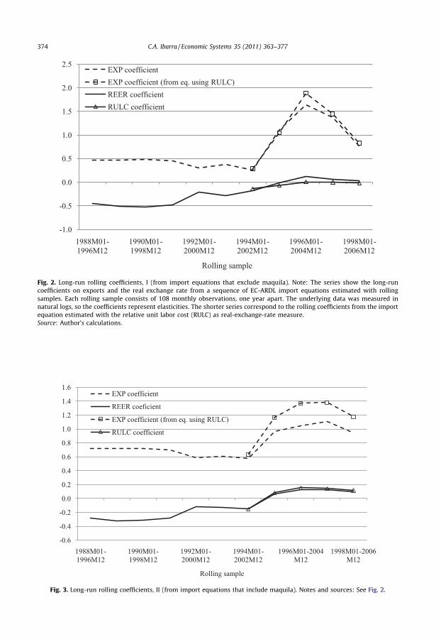
Finally, to reduce the probability that the observed changes in elasticities are an accident of thespecific sample partition, the import equation was estimated with rolling samples. Each sampleincludes 108 monthly observations, one year apart. The first sample runs from January 1988 toDecember 1996, the second from January 1989 to December 1997, and so on until the final sample,from January 1998 to December 2006.

For each rolling sample the EC-ARDL model yields a set of cointegration coefficients; Fig. 2 plotsthose for exports and the real exchange rate. The figure shows that the absolute value of the realexchange rate coefficient began to fall in the January 1992–December 2000 sample, while that ofexports began to rise in January 1995–December 2003. The same qualitative results are obtainedwhen relative unit costs rather than consumer prices are used as real exchange rate measure.

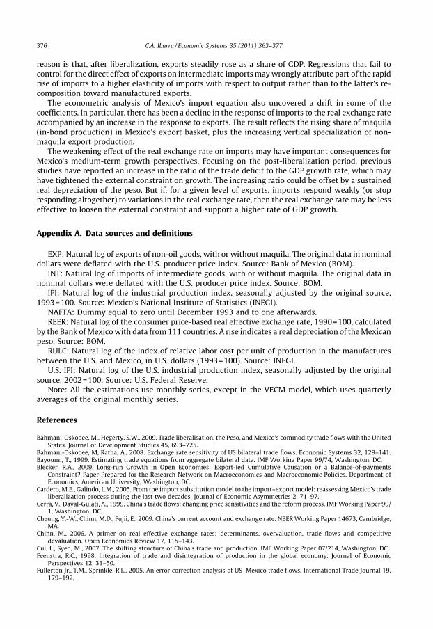
While the previous exercises excluded maquila to isolate the effects of vertical specialization in thenon-maquila sector, including maquila reinforces the estimation results (see Table 5 and Fig. 3). First,there is a decline in the (absolute value of the) real exchange rate coefficient from �0.25 before theenactment of NAFTA to �0.08 afterwards.

Second, estimating the import equation for the early (January 1988–December 1996) and late(January 1997–December 2006) samples shows a rise in the export coefficient (from 0.72 to 1.02),

Table 4Import cointegration equations, different periods (ex maquila). EC-ARDL estimations. Dependent variable: intermediate

imports, INT.

pre-NAFTA NAFTA Early Late

Sample 1988M1–1993M12a 1994M1–2006M12a 1988M1–1996M12,

n=108

1997M1–2006M12,

n=120


Industrial production, IPI 1.612 (3.559) 1.612 (3.559) 1.415 (2.373) 0.680 (1.228)

Exports, EXP 0.362 (3.281) 0.245 (�2.597)b 0.472 (3.403) 0.923 (3.532)

Real exchange rate, REER �0.447 (�3.048) �0.066 (2.635)b �0.443 (�2.235) 0.036 (0.495)



ADF �4.912 [0.000] �4.224 [0.001] �4.354 [0.001] �6.483 [0.000]

Phillips–Perron �4.802 [0.000] �9.640 [0.000] �6.592 [0.000] �6.422 [0.000]

Diagnostics

Jarque–Bera, x2 0.586 [0.746] 0.261 [0.878] 2.627 [0.269]

Breusch–Godfrey (6) 1.376 [0.226] 0.927 [0.480] 0.856 [0.531]

ARCH 0.637 [0.426] 0.004 [0.947] 3.362 [0.069]

RESET 0.275 [0.600] 1.271 [0.263] 0.073 [0.788]

Bounds tests

F-test 5.477 [4.35] (4.52) 4.609 [4.35] (4.52) 4.756 [4.35] (4.52)

t-test �5.189 [�3.78] �4.096 [�3.78] �3.901 [�3.78]


(1) The t-statistics (in parenthesis beside the long-run coefficients) correspond to the gi coefficients in Eq. (2) in the main text.

(2) The ADF (Augmented Dickey–Fuller) and Phillips–Perron tests include a constant and no trend. The number of lags in ADF

follows the Schwarz criterion (starting with a max of 12). P–P uses the Newey–West bandwidth. p-values in brackets.

(3) Diagnostics: The null hypotheses are that residuals are normally distributed (Jarque–Bera), with no serial correlation of up to

6th order (Breusch–Godfrey) and no ARCH errors, and that the equation passes Ramsey’s mis-specification test using the

squares of the fitted values (RESET). F-statistics with p-values in brackets.

(4) Bounds tests show 5% asymptotic upper critical values from Pesaran et al. (2001) in brackets and small-sample upper critical

values from Narayan (2005), for n=80 observations, in parenthesis.a Pre-NAFTA and NAFTA coefficients are calculated from a single equation that includes interactions with a NAFTA dummy, while ‘‘Early’’

and ‘‘Late’’ coefficients are calculated from two separate equations.b The t-stat corresponds to the gi coefficient on the interaction of the variable with the NAFTA dummy.


-1.0

-0.5

0.0

0.5

1.0

1.5

2.0

2.5

1988M01-1996M12

1990 M01-1998 M12

1992M01-2000M12

1994M01-2002M12

1996M01-2004M12

1998M01-2006M12

Rolling sample

EXP coefficie ntEXP coefficie nt (from eq. using RULC)REE R coefficie ntRULC coefficie nt

Fig. 2. Long-run rolling coefficients, I (from import equations that exclude maquila). Note: The series show the long-run

coefficients on exports and the real exchange rate from a sequence of EC-ARDL import equations estimated with rolling

samples. Each rolling sample consists of 108 monthly observations, one year apart. The underlying data was measured in

natural logs, so the coefficients represent elasticities. The shorter series correspond to the rolling coefficients from the import

equation estimated with the relative unit labor cost (RULC) as real-exchange-rate measure.


-0.6

-0.4

-0.2

0.0

0.2

0.4

0.6

0.8

1.0

1.2

1.4

1.6

1988M01-1996M12

1990 M01-1998 M12

1992M01-2000M12

1994M01-2002M12

1996M01-200 4M12

1998M01-200 6M12

Rolli ng sample

EXP coefficie nt

REE R coeficie nt

EXP coefficie nt (from eq. using RULC)

RULC coefficie nt

Fig. 3. Long-run rolling coefficients, II (from import equations that include maquila). Notes and sources: See Fig. 2.


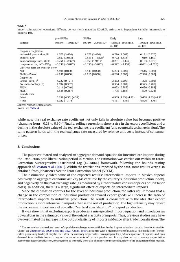
while now the real exchange rate coefficient not only falls in absolute value but becomes positive(changing from �0.28 to 0.10).8 Finally, rolling regressions show a rise in the export coefficient and adecline in the absolute value of the real exchange rate coefficient (and eventually a change in sign). Thesame pattern holds with the real exchange rate measured by relative unit costs instead of consumerprices.

5. Conclusions

The paper estimated and analyzed an aggregate demand equation for intermediate imports duringthe 1988–2006 post-liberalization period in Mexico. The estimation was carried out within an Error-Correction Autoregressive Distributed Lag (EC-ARDL) framework, following the bounds testingapproach of Pesaran et al. (2001). Within the restrictions imposed by the data, some results were alsoobtained from Johansen’s Vector Error Correction Model (VECM).

The estimation yielded some of the expected results: intermediate imports in Mexico dependpositively on aggregate economic activity (as captured by the country’s industrial production index),and negatively on the real exchange rate (as measured by either relative consumer prices or unit laborcosts). In addition, there is a large, significant effect of exports on intermediate imports.

Since the estimation controls for the level of industrial production, the latter result means that achange in the composition of industrial production toward export goods will increase the ratio ofintermediate imports to industrial production. The result is consistent with the idea that exportproduction is more intensive in imports than is the rest of production. The high intensity may reflectthe increasing importance of so-called ‘‘vertical specialization’’ of export production.

It was shown that excluding exports produces a mis-specified import equation and introduces anupward bias in the estimated value of the output elasticity of imports. Thus, previous studies may haveover-estimated the increase in the output elasticity of imports in Mexico after trade liberalization. The

Table 5Import cointegration equations, different periods (with maquila). EC-ARDL estimations. Dependent variable: Intermediate

imports, INT.

pre-NAFTA NAFTA Early Late

Sample 1988M1–1993M12a 1994M1–2006M12a 1988M1–1996M12,

n=108

1997M1–2006M12,

n=120


Industrial production, IPI 1.072 (3.454) 1.072 (3.454) 0.780 (2.067) 0.191 (0.670)

Exports, EXP 0.587 (3.963) 0.531 (�1.832)b 0.722 (3.835) 1.019 (4.160)

Real exchange rate, REER �0.251 (�2.377) �0.053 (1.941)b �0.281 (�2.147) 0.103 (2.376)



ADF �4.891 [0.000] �5.443 [0.000] �6.293 [0.000] �7.616 [0.000]

Phillips-Perron �4.857 [0.000] �9.110 [0.000] �6.286 [0.000] �7.580 [0.000]

Diagnostics

Jarque–Bera, x2 4.222 [0.121] 2.432 [0.296] 1.378 [0.502]

Breusch–Godfrey (6) 1.094 [0.367] 0.394 [0.881] 0.525 [0.788]

ARCH 0.111 [0.740] 0.073 [0.787] 0.020 [0.888]

RESET 1.535 [0.217] 1.795 [0.184] 1.520 [0.221]

Bounds tests

F-test 5.758 [4.35] (4.52) 4.959 [4.35] (4.52) 5.458 [4.35] (4.52)

t-test �5.022 [�3.78] �4.151 [�3.78] �4.526 [�3.78]


Notes: see Table 4.

8 The somewhat anomalous result of a positive exchange rate coefficient in the import equation has also been obtained for

China (see Cheung et al., 2009; Cerra and Dayal-Gulati, 1999), a country with a high presence of maquila-like production (the so-

called processing trade). It may be that, after the currency depreciates, firms prepare for a future expansion of exports, and thus

demand intermediate imports beyond the requirements of current production. It may also be that currency depreciation

accelerates export production, forcing firms to intensify their use of imports to respond quickly to the expansion of the market.


reason is that, after liberalization, exports steadily rose as a share of GDP. Regressions that fail tocontrol for the direct effect of exports on intermediate imports may wrongly attribute part of the rapidrise of imports to a higher elasticity of imports with respect to output rather than to the latter’s re-composition toward manufactured exports.

The econometric analysis of Mexico’s import equation also uncovered a drift in some of thecoefficients. In particular, there has been a decline in the response of imports to the real exchange rateaccompanied by an increase in the response to exports. The result reflects the rising share of maquila(in-bond production) in Mexico’s export basket, plus the increasing vertical specialization of non-maquila export production.

The weakening effect of the real exchange rate on imports may have important consequences forMexico’s medium-term growth perspectives. Focusing on the post-liberalization period, previousstudies have reported an increase in the ratio of the trade deficit to the GDP growth rate, which mayhave tightened the external constraint on growth. The increasing ratio could be offset by a sustainedreal depreciation of the peso. But if, for a given level of exports, imports respond weakly (or stopresponding altogether) to variations in the real exchange rate, then the real exchange rate may be lesseffective to loosen the external constraint and support a higher rate of GDP growth.

Appendix A. Data sources and definitions

EXP: Natural log of exports of non-oil goods, with or without maquila. The original data in nominaldollars were deflated with the U.S. producer price index. Source: Bank of Mexico (BOM).

INT: Natural log of imports of intermediate goods, with or without maquila. The original data innominal dollars were deflated with the U.S. producer price index. Source: BOM.

IPI: Natural log of the industrial production index, seasonally adjusted by the original source,1993=100. Source: Mexico’s National Institute of Statistics (INEGI).

NAFTA: Dummy equal to zero until December 1993 and to one afterwards.REER: Natural log of the consumer price-based real effective exchange rate, 1990=100, calculated

by the Bank of Mexico with data from 111 countries. A rise indicates a real depreciation of the Mexicanpeso. Source: BOM.

RULC: Natural log of the index of relative labor cost per unit of production in the manufacturesbetween the U.S. and Mexico, in U.S. dollars (1993=100). Source: INEGI.

U.S. IPI: Natural log of the U.S. industrial production index, seasonally adjusted by the originalsource, 2002=100. Source: U.S. Federal Reserve.

Note: All the estimations use monthly series, except in the VECM model, which uses quarterlyaverages of the original monthly series.

References

Bahmani-Oskooee, M., Hegerty, S.W., 2009. Trade liberalisation, the Peso, and Mexico’s commodity trade flows with the UnitedStates. Journal of Development Studies 45, 693–725.

Bahmani-Oskooee, M, Ratha, A., 2008. Exchange rate sensitivity of US bilateral trade flows. Economic Systems 32, 129–141.Bayoumi, T., 1999. Estimating trade equations from aggregate bilateral data. IMF Working Paper 99/74, Washington, DC.Blecker, R.A., 2009. Long-run Growth in Open Economies: Export-led Cumulative Causation or a Balance-of-payments

Constraint? Paper Prepared for the Research Network on Macroeconomics and Macroeconomic Policies. Department ofEconomics, American University, Washington, DC.

Cardero, M.E., Galindo, L.M., 2005. From the import substitution model to the import–export model: reassessing Mexico’s tradeliberalization process during the last two decades. Journal of Economic Asymmetries 2, 71–97.

Cerra, V., Dayal-Gulati, A., 1999. China’s trade flows: changing price sensitivities and the reform process. IMF Working Paper 99/1, Washington, DC.

Cheung, Y.-W., Chinn, M.D., Fujii, E., 2009. China’s current account and exchange rate. NBER Working Paper 14673, Cambridge,MA.

Chinn, M., 2006. A primer on real effective exchange rates: determinants, overvaluation, trade flows and competitivedevaluation. Open Economies Review 17, 115–143.

Cui, L., Syed, M., 2007. The shifting structure of China’s trade and production. IMF Working Paper 07/214, Washington, DC.Feenstra, R.C., 1998. Integration of trade and disintegration of production in the global economy. Journal of Economic

Perspectives 12, 31–50.Fullerton Jr., T.M., Sprinkle, R.L., 2005. An error correction analysis of US–Mexico trade flows. International Trade Journal 19,

179–192.


Garces-Dıaz, D., 2008. An empirical analysis of the economic integration between Mexico and the U.S. and its connection withreal exchange rate fluctuations (1980–2000). International Trade Journal 22, 484–513.

Guerrero de Lizardi, C., 2003. Modelo de crecimiento restringido por la balanza de pagos. Evidencia para Mexico 1940–2000. ElTrimestre Economico 70, 253–273.

Harris, R., Sollis, R., 2003. Applied Time Series Modelling and Forecasting. Wiley, Chichester.Haugh, D., Jamin, R., Rocha, B., 2008. Maximising Mexico’s gains from integration in the world economy. OECD Economics

Department Working Paper 657, Paris.Hummels, D., Ishii, J., Yi, K.-M., 2001. The nature and growth of vertical specialization in world trade. Journal of International

Economics 54, 75–96.Ibarra, C.A., 2011. Monetary policy and real currency appreciation: A BEER model for the Mexican peso. International Economic

Journal 25, 95–110.Ibarra, C.A., 2010a. Maquila, currency misalignment, and export-led growth in Mexico. CEPAL Review, forthcoming.Ibarra, C.A., 2010b. A note on intermediate imports and the BPCG model in Mexico. Economic Change and Restructuring,

forthcoming.Ibarra, C.A., 2003. Sluggish growth, trade liberalization and the Mexican disease: a medium-term macroeconomic model with

an application to Mexico. International Review of Applied Economics 17, 269–292.Irandoust, M., Ekblad, K., Parmler, J., 2006. Bilateral trade flows and exchange rate sensitivity: evidence from likelihood-based

panel cointegration. Economic Systems 30, 170–183.Johansen, S., 2002. A small sample correction for the test of cointegrating rank in the vector autoregressive model. Econometrica

70, 1929–1961.Juselius, K., 2006. The Cointegrated VAR Model: Methodology and Applications. Oxford University Press, Oxford.Kemme, M.D., Roy, S., 2006. Real exchange rate misalignment: Prelude to crisis? Economic Systems 30, 207–230.Lederman, D., Menendez, A.M., Perry, G., Stiglitz, J., 2000. Mexico: five years after the crisis. In: Paper Prepared for the World

Bank ABCDE Conference. World Bank, Washington, DC.Lommatzsch, K., Tober, S., 2004. What is behind the real appreciation of the accession countries’ currencies? An investigation of

the PPI-based real exchange rate. Economic Systems 28, 383–403.Lopez, J., Cruz, A., 2000. Thirlwall’s law and beyond: the Latin American experience. Journal of Post Keynesian Economics 22,

477–495.McDaniel, C.A., Agama, L.-A., 2003. The NAFTA preference and US–Mexico trade: aggregate-level analysis. World Economy 26,

939–955.Moissinac, V., 2006. A survey of conditions for growth in Mexico, in international perspective. In: IMF (Eds.), Mexico: Selected

Issues. IMF, Washington, DC, pp. 2–230.Moreno-Brid, J.C., 1999. Mexico’s economic growth and the balance of payments constraint: a cointegration analysis.

International Review of Applied Economics 13, 149–159.Moreno-Brid, J.C., Ros, J., 2009. Development and Growth in the Mexican Economy: A Historical Perspective. Oxford University

Press, Oxford.Moreno-Brid, J.C., Santamarıa, J., Rivas, J.C., 2005. Industrialization and economic growth in Mexico after NAFTA: the road

travelled. Development and Change 36, 1095–1119.Narayan, P.K., 2005. The saving and investment nexus for China: evidence from cointegration tests. Applied Economics 37,

1979–1990.Ocegueda, J., 2000. La hipotesis del crecimiento restringido por la balanza de pagos. Una evaluacion de la economıa mexicana

1960–1997. Investigacion Economica 60, 91–122.Oomes, N., 2005. Maintaining competitiveness under equilibrium real appreciation: the case of Slovakia. Economic Systems 29,

187–204.Organization for Economic Cooperation and Development (OECD), 2005. The benefits of liberalizing product markets and

reducing barriers to international trade and investment in the OECD. OECD Economics Department working paper 463,Paris.

Pacheco-Lopez, P., 2005. The impact of trade liberalization on exports, imports, the balance of payments and growth: the case ofMexico. Journal of Post Keynesian Economics 27, 595–619.

Pacheco-Lopez, P., Thirlwall, A.P., 2007. Trade liberalization and the trade-off between growth and the balance of payments inLatin America. International Review of Applied Economics 21, 469–490.

Pesaran, M.H., Shin, Y., Smith, R.J., 2001. Bounds testing approaches to the analysis of level relationships. Journal of AppliedEconometrics 16, 289–326.

Pesaran, M.H., Shin, Y., Smith, R.J., 2000. Structural analysis of vector error correction models with exogenous I(1) variables.Journal of Econometrics 97, 293–343.

Ros, J., 1994. Mexico’s trade and industrialization experience since 1960: a reconsideration of past policies and assessment ofcurrent reforms. In: Helleiner, G. (Ed.), Trade Policy and Industrialization in Turbulent Times. Routledge, London, pp. 170–216.

Sanchez, F., Fernandez, M., Perez, E., 1994. La Polıtica Industrial ante la Apertura. Fondo de Cultura Economica, Mexico City.Sissoko, Y., Dibooglu, S., 2006. The exchange rate system and macroeconomic fluctuations in Sub-Saharan Africa. Economic

Systems 30, 141–156.World Trade Organization (WTO), 2008a. Trade policy review. Report by the Mexican Government, Trade Policy Review Body,

WT/TPR/G/195, Geneva.World Trade Organization (WTO), 2008b. Trade policy review. Report by the Secretariat, Trade Policy Review Body, WT/TPR/S/

195, Geneva.


Documents

Import elasticities and the external constraint in Mexico