Embed Size (px)
Citation preview

arX
iv:1
002.
2897
v1 [
cs.A
I] 1
5 F
eb 2
010
Model-Driven Constraint Programming
Raphael ChenouardCNRS, LINA, Universite de Nantes,
Laurent GranvilliersCNRS, LINA, Universite de Nantes,
Ricardo SotoCNRS, LINA, Universite de Nantes,
France.Pontificia Universidad Catolica de
Valparaıso, [email protected]
AbstractConstraint programming can definitely be seen as a model-drivenparadigm. The users write programs for modeling problems. Theseprograms are mapped to executable models to calculate the solu-tions. This paper focuses on efficient model management (defini-tion and transformation). From this point of view, we propose torevisit the design of constraint-programming systems. A model-driven architecture is introduced to map solving-independent con-straint models to solving-dependent decision models. Several im-portant questions are examined, such as the need for a visualhigh-level modeling language, and the quality of metamodeling tech-niques to implement the transformations. A main result is the s-
COMMA platform that efficiently implements the chain from mod-eling to solving constraint problems.
Categories and Subject Descriptors D.3.2 [Programming Lan-guages]: Language Classifications—Constraint and logic lan-guages; D.2.2 [Software Engineering]: Design Tools and Tech-niques—User interfaces; D.3.3 [Programming Languages]: Lan-guage Constructs and Features—Classes and objects, Constraints
General Terms Languages
Keywords Constraint Modeling Languages, Constraint Program-ming, Metamodeling, Model Transformation
1. IntroductionIn constraint programming (CP), programmers define a model of aproblem usingconstraintsover variables. The variables may takevalues from domains, typically boolean, integer, or rational values.The solutions to be found are tuples of values of the variables satis-fying the constraints. The search process is performed by powerfulsolving techniques, for instance backtracking-like procedures andconsistency algorithms to explore and reduce the space of potentialsolutions. In the past, CP has been shown to be efficient for solvinghard combinatorial problems.
CP systems evolved from the early days of constraint logic pro-gramming (CLP). In a CLP system, the constraint language is em-bedded in a logic language, and the solving procedure combines theSLD-resolution with calls to constraint solvers [15]. The logic lan-guage can be replaced with any computer programming language
Permission to make digital or hard copies of all or part of this work for personal orclassroom use is granted without fee provided that copies are not made or distributedfor profit or commercial advantage and that copies bear this notice and the full citationon the first page. To copy otherwise, to republish, to post on servers or to redistributeto lists, requires prior specific permission and/or a fee.
PPDP’08, July 16–18, 2008, Valencia, Spain.Copyright c© 2008 ACM 978-1-60558-117-0/08/07. . . $5.00
(e.g. C++ in ILOG Solver [26] or Java in Gecode/J [12]) and eventerm rewriting [11]. It turns out that the programming task may behard, especially for non experts of CP or computer programming.In this approach, modeling concerns are not enough to write pro-grams, and it is often mandatory to deal with the encoding aspectsof the host language or to tune the solving strategy. In responseto this problem, almost pure modeling languages have been built,such as OPL [30] and Zinc [27].
The design of the last generation of CP systems has been gov-erned by the idea of separating modeling and solving capabilities(e.g. Essence [9] and MiniZinc [21]). The system architecture hasthree layers, including the modeling language, the solvers, and amiddle tool composed by a set of solver-translators implementingthe mappings. In particular, this approach gives importantbene-fits: The full expressiveness of CP is supported by a unique high-level modeling language, which is expected to be simple enough fornon experts. The user is able to process one model with differentsolvers, a crucial feature for easy and fast problem experimentation.The platform is open to plug new solvers.
Our work follows this solver-independent idea, but under aModel-Driven Development (MDD) approach [24], which is well-known in the software engineering sphere. General requirementshave been defined for MDD architectures in order to define concisemodels, to enable interoperability between tools, and to easily pro-gram mappings between models. The classical MDD infrastructureuses as base element the notion of a metamodel, which allows oneto clearly define the concepts appearing in a model.
In this paper, the MDD approach is applied to a CP system.The goal is to implement the chain from modeling to solving con-straints. Our approach is to transform user solving-independentmodels defined through a visual modeling language to solver (ex-ecutable) models using a metamodeling strategy. CP concepts likedomains, variables, constraints, and relations between them are de-fined in a metamodel, and thus the transformation rules are able tomap these concepts from a source language to a target one. It resultsin a flexible and extensible architecture, robust enough to supportchanges at the mapping tool level. Moreover, we believe thatthestudy of metamodels for CP is of interest.
These ideas have been implemented in thes-COMMA plat-form [28]. The front tool allows users to graphically define con-straint models. It is made on top of a general object-oriented con-straint language [29]. Many solvers have been plugged in theplat-form such as ECLiPSe [31], Gecode/J [12], GNU Prolog [6] andRealpaver [14]. Upgrades are supported at the mapping tool,newsolver-translators can be added by means of the AMMA plat-form [20].
The language for stating constraints ins-COMMA is clearly notthe novel part of the platform, in fact it includes typical and state-of-the-art modeling constructs and features. Novelty arises from

the introduction of a solver-independent visual language –whichwe believe is intuitive and simple enough for non experts –, andthe use of a MDD approach involving metamodeling techniquestoimplement the mappings.
The outline of this paper is as follows. The MDD architectureproposed is introduced in Section 2. Thes-COMMA modeling lan-guage and the associated graphical interface are presentedin Sec-tion 3. The mapping tool and the metamodeling techniques used todevelop solver-translators are explained in Section 4. Some exper-imental results are then discussed in Section 5. The relatedworkand conclusion follows.
2. A MDD approach for CPModel-Driven Engineering (MDE) aims to consider models as firstclass entities. A model is defined according to the semanticsof amodel of models, also called ametamodel. A metamodel describesthe concepts appearing in a model, but also the links betweentheseconcepts, such as: inheritance, composition or simple association.
Figure 1 depicts a general Model-Driven Architecture (MDA)for model transformation. Level M1 holds the model. Level M2describes the semantic of the level M1 and thus identifies conceptshandled by this model through a metamodel. Level M3 is thespecification of level M2 and is self-defined. Transformation rulesare defined to translate models from a source model to a targetone,the semantic of these rules is also defined by a metamodel.
A major strength of using this metamodeling approach is thatmodels are concisely represented by metamodels. This allows oneto define transformation rules that only operate on the conceptsof metamodels (at the M2 level of the MDA approach), not onthe concrete syntax of a language. Syntax concerns are definedindependently (we illustrate this in Section 4). This separation isa great advantage for a clearly definition of transformationrulesand grammar descriptions, which are the base of our mapping tool.
Figure 1. A general MDA for model transformation.
Let us now illustrate how this approach is implemented in ourplatform. Figure 2 shows the MDDs-COMMA architecture, whichis composed by two main parts, a modeling tool and a mappingtool.
The s-COMMA GUI is our modeling tool, and it allow users tostate constraint models using visual artifacts. An exactlytextualrepresentation of this language is also provided (for who does notwant to use visual artifacts). Both languages are solver-independentand are designed conform to the same metamodel (see Section 3).The output of thes-COMMA GUI is Flat s-COMMA an interme-diate language which is still solver-independent but, in terms ofabstraction is closer to the solver level. The goal is to simplify thedevelopment of solver-translators.Flat s-COMMA is also designedconform to a metamodel (see Section 3.3).
The mapping tool is composed by a set of solver-translators.Solver-translators are designed to match the metamodel conceptsof Flat s-COMMA to the concepts of the solver metamodel (seeSection 4). This process is defined conform to the general MDAfor model transformation.
Figure 2. The MDD architecture of s-COMMA.
The s-COMMA GUI is written in Java (about 30000 lines) andtranslators are developed using the AMMA platform. The wholesystem allows to perform the complete process from visual modelsto solver models. The system involves several metamodels: an s-
COMMA metamodel, aFlat s-COMMA and solver metamodels.The s-COMMA metamodel has been built just for defining theconcepts of thes-COMMA textual and visual language, it is notused to maps-COMMA to Flat s-COMMA. For this task we alreadyhave an efficient translator. Our key aim of using metamodelingtechniques is to provide an easier way to develop new solver-translators, compared to the task of writing translators byhand.
In the following two sections we present the main parts of thisarchitecture: The modeling and the mapping tool, respectively.
3. Modeling ToolWe have built ours-COMMA GUI modeling tool on top of thes-COMMA language. Thes-COMMA language is defined through itsmetamodel and it has been designed to represent the conceptsofconstraint problems, also called constraint satisfactionproblems(CSPs). In this metamodel, the CSP concepts such as variables anddomains have been merged with object-oriented concepts in orderto state CSPs using an object-oriented style. The result is an object-oriented visual language for modeling CSPs. These decisions aresupported by the following benefits:
• A problem is generally composed of several parts which mayrepresent objects. They are naturally specified through classes.Thus, we obtain a more modular model, instead of forcingmodelers to state the entire problem in a single block of code.
• We gain similar benefits – constraint and variable encapsula-tion, composition, inheritance, reuse – to those gained by writ-ing software in a object-oriented programming language.
• Visual artifacts are more intuitive to use and give a clearerviewof the complete structure of the problem.
Figure 3 illustrates the main concepts of thes-COMMA meta-model using UML class diagram notation. The role of each one ofthese concepts is explained in the following paragraphs.
3.1 s-COMMA models
The s-COMMA metamodel defines the concepts appearing ins-
COMMA models. Thus, conform to this metamodel ans-COMMA
model must be composed by two main parts, the model and data.The model describes the structure of the problem and the datacon-tain the constant values used by the model. In ours-COMMA GUI
front tool this problem’s structure is represented by classartifacts

and the data concept is represented by the data artifact1 (see Fig-ure 4).
Figure 3. s-COMMA Metamodel.
3.1.1 Class artifacts
Class artifacts have by default three compartments, the upper com-partment for the class name, the middle compartment for attributesand the bottom one for constraint zones. By clicking on the classartifact its specification can be opened to define its class name, theirattributes and constraint zones. Relationships can be usedto defineinheritance (a subclass inherits all attributes and constraint zones ofits superclass) or composition between classes.
3.1.2 Data artifacts
Data artifacts have two compartments, one for the file name andanother for both the constants and variable-assignments. Constants,also called data variables can be defined with a real, integeror enu-meration type. Arrays of one dimension and arrays of two dimen-sions of constants are allowed. Variable-assignment correspondsto the assignment of a value to a variable of an object. Variable-assignments can also be performed if objects are inside an array(see an example in Section 3.2).
Figure 4. Class artifact used in s-COMMA GUI
1 Artifacts used on thes-COMMA GUI have been adapted from the classartifact provided by the UML Infrastructure Library Basic Package. Thisadaptation is completely allowed by the UML InfrastructureSpecifica-tion [23].
3.1.3 Attributes
Attributes may represent decision variables, sets, objects or arrays.Decision variables can be defined by an integer, real or booleantype. Sets can be composed of integers or enumeration values.Objects are instances of classes which must be typed with theirclass name. Arrays of one and two dimensions are allowed, theycan contain decision variables, sets or objects. Decision variables,sets and arrays can be constrained to a determined domain.
3.1.4 Constraint Zones
Constraint zones are used to group constraints encapsulating theminside a class. A constraint zone is stated with a name and it cancontain the following elements:
• Constraints: Typical operations and relations are providedto post constraints. For example, comparison relations (<,>,
<=,>=,=,<>), arithmetic operations (+,*, -,/), logical re-lations (and,or,xor, ->,<-,<->), and set operations (in,subset, superset, union, diff, symdiff, intersection,
cardinality).
• Statements:Forall and conditional statements are supported.The forall (e.g.forall(i in 1..5)) is stated by declaring aloop-variable (i) and the set of values to be traversed (1..5).A loop-variable is a local variable and it is valid just inside theloop where it was declared. Conditionals are stated by meansofif-else expressions. For instance,if(a) b else c; wherea isthe condition, which can includes decision variables; andb andc are the alternatives, which may be statements or constraints.
• Objective: objective functions are allowed and they can bestated by tagging the expression involved with the selectedoption (e.g.[minimize] x+y+z;).
• Global Constraints: a basic set of global constraints (e.g. alldif-ferent, cumulatives) is supported. Additional constraints can beintegrated to this basic set by means of extension mechanisms(for details refer to [29]).
3.2 The stable marriage problem
Let us now illustrate some of these concepts in thes-COMMA GUI
by means of the stable marriage problem.
Figure 5. The stable marriage problem on the s-COMMA GUI
Consider a group ofn women and a group ofn men who mustmarry. Each women has a preference ranking for her possible hus-band, and each men has a preference ranking for his possible wife.

The problem is to find a matching between the groups such that themarriages are stable i.e., there are no pair of people of opposite sexthat like each other better than their respective spouses.
Figure 5 shows a snapshot of thes-COMMA GUI where thestable marriage problem is represented by a class diagram. Thisdiagram is composed by three classes, one class to representmen,one to represent women, and a main class to describe the stablemarriages. Once the user states a visual artifact, the correspondings-COMMA textual version is automatically generated on the right-panel of the tool. For readability we illustrate the textualversion ofthe problem in Fig. 6
//Model file
1. import StableMarriage.dat;2.3. class StableMarriage {
4.5. Man man[menList];
6. Woman woman[womenList];7.
8. constraint matchHusbandWife {9. forall(m in menList)10. woman[man[m].wife].husband = m;
11.12. forall(w in womenList)
13. man[woman[w].husband].wife = w;14. }15.
16. constraint forbidUnstableCouples {17. forall(m in menList){
18. forall(w in womenList){19. man[m].rank[w] < man[m].rank[man[m].wife] ->
20. woman[w].rank[woman[w].husband] < woman[w].rank[m];21.22. woman[w].rank[m] < woman[w].rank[woman[w].husband] ->
23. man[m].rank[man[m].wife] < man[m].rank[w];24. }
25. }26. }
27.}28.29. class Man {
30. int rank[womenList];31. womenList wife;
32. }33.34. class Woman {
35. int rank[menList];36. menList husband;
37. }
//Data file1. enum menList := {Richard,James,John,Hugh,Greg};2. enum womenList := {Helen,Tracy,Linda,Sally,Wanda};
3. Man StableMarriage.man :=[Richard: {[Helen:5 ,Tracy:1, Linda:2, Sally:4, Wanda:3],_},
James : {[Helen:4 ,Tracy:1, Linda:3, Sally:2, Wanda:5],_},John : {[Helen:5 ,Tracy:3, Linda:2, Sally:4, Wanda:1],_},Hugh : {[Helen:1 ,Tracy:5, Linda:4, Sally:3, Wanda:2],_},
Greg : {[Helen:4 ,Tracy:3, Linda:2, Sally:1, Wanda:5],_}];
4. Woman StableMarriage.woman :=[Helen: {[Richard:1, James:2, John:4, Hugh:3, Greg:5],_},
Tracy: {[Richard:3, James:5, John:1, Hugh:2, Greg:4],_},Linda: {[Richard:5, James:4, John:2, Hugh:1, Greg:3],_},Sally: {[Richard:1, James:3, John:5, Hugh:4, Greg:2],_},
Wanda: {[Richard:4, James:2, John:3, Hugh:5, Greg:1],_}];
Figure 6. An s-COMMA model for the stable marriage problem.
The class representing men (at line 29 in the model file) iscomposed by one array containing integer values which representsthe preferences of a man, the array is indexed by the enumerationtype womenList (at line 2 in the data file), thereby the 1st indexof the array isHelen, the 2nd isTracy, the third isLinda andso on. Then, an attribute calledwife is defined (line 31), which
represents the spouse of an object man. This variable haswomenList
as a type which means that its domain is given by the enumerationwomenList. The definition of the classWomen is analogous.
The classStableMarriage has a more complex declaration. Wefirst define two arrays, one calledman which contains objects ofthe classMan and other which contains objects of the classWoman.Each one represents the group of men and the group of women,respectively. The composition relationship between classes can beseen on the class diagram.
At line 8 a constraint zone calledmatchHusbandWife is stated.In this constraint zone, twoforall loops including a constraintare posted to ensure that the pairs man-wife match with the pairswoman-husband. TheforbidUnstableCouples constraint zonecontains two loops including two logical formulas to ensurethatmarriages are stable.
The data file is called by means of an import statement (atline 1). This file contains two enumeration types,menList andwomenList, which have been used in the model as a type, for in-dexing arrays, and as the set of values that loop-variables must tra-verse.StableMarriage.man is a variable-assignment for the arraycalledman defined at line 5 in the model file.
This variable-assignment is composed by five objects (enclosedby ‘{}’), one for each men of the group. Each of these objects hastwo elements, the first element2 is an array (enclosed by‘[ ]’).This array sets the preferences of a men, assigning the values to thearrayrank of a Man object (e.g. Richard prefers Tracy 1st, Linda2nd, Wanda 3rd, etc).
The second element is an underscore symbol (’’). This symbolis used to omit assignments, so the variablewife remains as adecision variable of the problem i.e., a variable for which the solvermust search a solution.
3.3 Flat s-COMMA models
Before explaining hows-COMMA models are mapped to theirequivalent solver models, let us introduce the intermediate Flat s-
COMMA language.
Figure 7. Flat s-COMMA Metamodel.
Flat s-COMMA has been designed to simplify the transforma-tion process froms-COMMA models to solver models. InFlat s-
COMMA much of the constructs supported bys-COMMA are trans-formed to simpler ones, in order to be closer to the form requiredby classical solver languages.Flat s-COMMA is also defined by ametamodel.
Figure 7 illustrates the main elements of theFlat s-COMMA
metamodel, where manys-COMMA concepts have been removed.Now, the metamodel is mainly a definition of a problem composedby variables (decision variables) and constraints.
In order to transforms-COMMA toFlat s-COMMA, several stepsare involved, which are explained in the following.
2 Let us note that we use standard modeling variable-assignments, that is,assignments are performed respecting the order of the class’ attributes: thefirst element of the variable-assignment is matched with thefirst attributeof the class, the second element of the variable-assignmentwith the secondattribute of the class and so on.

• Enumeration substitution: In general solvers do not supportnon-numeric types. So, enumerations are replaced by integervalues. However, enumeration values are stored to show theresults in the correct format.
• Data substitution: Data variables stated in the model file arereplaced by their corresponding values i.e., the value defined inthe data file.
• Loop unrolling: Loops are not widely supported by solvers,hence we generate an unrolled version of the forall loop.
• Flattening composition: The hierarchy generated by composi-tion is flattened. This process is done by expanding each objectdeclared in the main class adding its attributes and constraintsin theFlat s-COMMA file. The name of each attribute has a pre-fix corresponding to the concatenation of the names of objectsof origin in order to avoid name redundancy.
• Conditional removal: Conditional statements are transformed tological formulas. For instance,if a then b else c is replacedby (a ⇒ b) ∧ (a ∨ c).
• Logic formulas transformation: Some logic operators are notsupported by solvers. For example, logical equivalence (a ⇔
b) and reverse implication (a ⇐ b). We transform logicalequivalence expressing it in terms of logical implication ((a ⇒
b)∧ (b ⇒ a)). Reverse implication is simply inverted (b ⇒ a).
1. variables:2.
3. womenList man_wife[5] in [1,5];4. menList woman_husband[5] in [1,5];
5.6. constraints:
7.8. woman_husband[man_wife[1]]=1;9. woman_husband[man_wife[2]]=2;
10. woman_husband[man_wife[3]]=3;11. ...
12.13. man_wife[woman_husband[1]]=1;14. man_wife[woman_husband[2]]=2;
15. man_wife[woman_husband[3]]=3;16. ...
17.18. 5<man_1_rank[man_wife[1]] ->
19. woman_1_rank[woman_husband[1]]<1;20. 1<woman_1_rank[woman_husband[1]] ->21. man_1_rank[man_wife[1]]<5;
22.23. 1<man_1_rank[man_wife[1]] ->
24. woman_2_rank[woman_husband[2]]<3;25. 3<woman_2_rank[woman_husband[2]] ->
26. man_1_rank[man_wife[1]]<1;27. ...28.
29. enum-types:30.
31. menList := {Richard,James,John,Hugh,Greg};32. womenList := {Helen,Tracy,Linda,Sally,Wanda};
Figure 8. The Flat s-COMMA model of the stable marriage prob-lem.
Figure 8 depicts theFlat s-COMMA model of the stable mar-riage problem. The file is composed of two main parts, variablesand constraints. Variables at lines 3-4 are generated by theflatten-ing composition process. The arrayman composed by objects oftypeMan is decomposed and transformed to a single array of deci-sion variables. The arrayman wife contains the decision variableswife of the original arrayman; and the arraywoman husband con-tains the decision variableshusband of the original arraywoman. Thearrays rank of both objectsMan andWoman are not considered as de-cision variables since they have been filled with constants (at lines
3-4 of the data file in Figure 6). The size of the arrayman wife is 5,this value is given by the enumeration substitution step which setsthe size of the array with the size of the enumerationmenList (5).The domain[1,5] is also given by this step which states as domainan integer range corresponding to the number of elements of theenumeration used as a type (womenList) by the attributewife. Thetype of both arrays is maintained to give the solutions in theenu-meration format. These values are stored in the blockenum-types.Lines 8-15 come from the loop unrolling phase of the forall state-ments of thematchHusbandWife constraint zone. Likewise, lines18-26 are generated by the loops offorbidUnstableCouples. Inthese constraints, the data substitution step has replacedseveralconstants with their corresponding integer values.
4. Mapping ToolIn this section we explain the mechanisms provided by the MDDapproach to develop our solver-translators. These translators aredesigned to perform the mapping fromFlat s-COMMA to solvermodels. We use the AMMA platform as our base tool to build them.
The AMMA platform allows one to develop this task by meansof two languages: KM3 [18] and ATL [17]. KM3 is used to definemetamodels, and ATL is used to describe the transformation rulesand also to generate the target file.
4.1 KM3
The Kernel Meta Meta Model (KM3) is a language to define meta-models. KM3 has been designed to support most metamodelingstandards and it is based on the simple notion of classes to de-fine each one of the concepts of a metamodel. These concepts willthen be used by the transformation rules and to generate the targetfile. Figure 9 illustrates an extract of theFlat s-COMMA metamodelwritten in KM3.
1. class Problem {2. attribute name : String;
3. reference variables[1-*] container : Variable;4. reference constraints[0-*] container : Constraint;5. reference enumTypes[0-*] container : EnumType;
6. }7.
8. class Variable {9. attribute name : String;
10. attribute type : String;11. reference array [0-1] container : Array;12. reference domain container : Domain;
13. }14.
15. class Array {16. attribute row : Integer;17. attribute col[0-1] : Integer;
18. }
Figure 9. An extract of the Flat s-COMMA KM3 metamodel.
The Flat s-COMMA KM3 metamodel states that the conceptProblem is composed of one attribute and three references. Theattributename at line 2 represents the name of the model and itis declared with the basic typeString. Line 3 simply states thatthe classProblem is composed by a set of objects of the classVariable. The reserved wordreference is used to declare linkswith instances of other classes and the statement[1-*] definesthe multiplicity of the relationship. If the multiplicity statement isomitted the relationship is defined as[1-1]. Lines 4-5 are similarand define that the classProblem is also composed byconstraintsandenumTypes (values stored by the enumeration substitution step).Remaining classes are defined in the same way.

4.2 ATL
The Atlas Transformation Language (ATL) allow us to define trans-formation rules according to one or several metamodels. Therulesclearly state how concepts from source metamodels are matchedto concepts of the target ones. Figure 10 shows some of the ATLrules used to transform the concepts of theFlat s-COMMA meta-model to the concepts of the Gecode/J metamodel. The metamodelof Gecode/J is not presented here since it is very close to theFlat s-
COMMA metamodel. Indeed, most CP solver languages are used toexpress quite the same concepts andFlat s-COMMA is designed tobe as close as possible from the solving level. This is a greatassetbecause transformation rules become simple: we mainly needoneto one transformations.
1. module FlatsComma2GecodeJ;
2. create OUT : GecodeJ from IN : FlatsComma;3.
4. rule Problem2Problem {5. from6. s : FlatsComma!Problem (
7. )8. to
9. t : GecodeJ!Problem(10. name <- s.name,11. variables <- s.variables,
12. constraints <- s.constraints,13. enumTypes <- s.enumTypes
14. )15. }
16.17. rule Variable2Variable {18. from
19. s : FlatsComma!Variable (20. not s.isArrayVariable
21. )22. to23. t : GecodeJ!Variable (
24. name <- s.name,25. type <- s.type,
26. domain <- s.domain27 )
28. }29.30. helper context FlatsComma!Variable def:
31. isArrayVariable : Boolean=32. not self.array.oclIsUndefined();
Figure 10. ATL rules for transformation from Flat s-COMMA toGecode/J.
The first line of this file specifies the name of the transformation.A module is used to define and regroup a set of rules and helpers.Rules define the mappings, and helpers allow to define factorizedATL code that can be called from different points of the ATL file(they can be viewed as the ATL equivalent to Java methods).
Line 2 states the target (create) and source metamodels (from).The first rule presented is calledProblem2Problem and definesthe matching between the conceptsProblem expressed inFlat s-
COMMA and Gecode/J. The source elements are stated with thereserved wordfrom and the target ones with the reserved wordto.These elements are declared like variables with a name (s,t) and atype corresponding to a class in a metamodel (FlatsComma!Problem,
GecodeJ!Problem). In the target part of the rule the name at-tribute of theFlat s-COMMA problem is assigned to the Gecode/Jname (name <- s.name), this is just an string assignment. How-ever, the following two statement are assignments between con-cepts that are defined asreference in the metamodel. So, theyneed a specific rule to carry out the transformation. For instance,the Flat s-COMMA KM3 metamodel defines that the referencevariables is composed by a set ofVariable elements. Thus, thestatement (variables <- s.variables) calls implicitly the rule
Variable2Variable, which defines the match between each ele-ment of objectsVariable. It can be highlighted that the ATL enginerequires a unique name for each rule and a unique matching case:from and to blocks. When several rules can be applied a guard(the boolean test in line 20) over the from statement must removechoice ambiguities.
TheVariable2Variable rule matches three elements. The firsttwo statements are simple string assignments and the last one is areference assignment. Let us remark that a second rule to processarray variables has been defined (but not presented here) whichincludes an additional statement for the array element. These tworules are distinguished according to complementary guardsoverthe source block using the helperisArrayVariable. Guards act asfilter on the source variable instances to process. The presentedhelperisArrayVariable applies on variable instances inFlat s-
COMMA models and returns true when the instance contains anarray element. ATL inherits from OCL [22] syntax and semantics;and most OCL functions and types are available within ATL.
Although the rules used here are not complex, ATL is able toperform more difficult rules. For instance, the most difficult rule wedefined, was the transformation rule fromFlat s-COMMA matrixcontaining sets, which must be unrolled in the ECLiPSe models(since set matrix are not supported). This unroll process iscarriedout by defining a single set in ECLiPSe for each cell in the matrix.The name of each single variable is composed by the name of thematrix, and the corresponding row and column index.
1. rule Problem2Problem {
2. from3. s : FlatsComma!Problem (
4. s.hasSetMatrix5. )6. to
7. t : ECLiPSe!Problem (8. name <- s.name,
9. constraints <- s.constraints,10. enumTypes <- s.enumTypes
11. )12. do {13. t.variables <- s.variables->collect(e|
14. if e.isSetMatrix() then15. thisModule.getMatrixCells(e)->collect(f|
16. thisModule.SetMatrixVariable2Variable(f.var,f.i,f.j)17. )18. else
19. e20. endif
21. )->flatten();22. }
23. }24.25. rule SetMatrixVariable2Variable(var : FlatsComma!Variable,
26. i : Integer, j : Integer) {27. to
28. t : ECLiPSe!Variable(29. name <- var.name + i.toString() + ’_’ + j.toString(),30. type <- var.type,
31. domain <- var.domain,32. )
33. do {34. t;
35. }36. }
Figure 11. ATL rules for decomposing matrix containing sets.
Figure 11 shows the ruleProblem2Problem defined for ECLiPSe,this rule has a condition (line 4) to check whether set matrixaredefined in the model. If the condition is true,name, constraintsandenumTypes are matched normally, butvariables has a specialprocedure to decompose the set matrix.
This procedure begins at line 12 with ado block. In this block,the collect loop iterates over the variables. Then, each of these

variables (e) is checked to determine whether it has been defined asa set matrix (line 14). If this occurs, the helpergetMatrixCells(e)
calculates the set of tuples corresponding to all the cells of thematrix (thisModule is used to call explicitly helpers or rules).Each tuple is composed of theFlat s-COMMA variable (f.var),a row index (f.i) and a column index (f.j). Then, the ruleSetMatrixVariable2Variable is applied to each tuple in orderto generate the ECLiPSe variables. This rule does not contain asource block since the source elements are the input parameters.The rule sets to the attributename, the concatenation of the nameof the matrix with the respective row (i.toString()) and column(j.toString()). Attributestype anddomain are also matched. Fi-nally, flatten() is an OCL inherited method used to match thegenerated set of variables witht.variables.
ATL is also used to generate the solver target file. This ispossible by defining a new ATL file (called generically ATL2Text)where we can embed the concepts of the metamodel in the syntaxof the target file. This is done by means of a querying facilitythatenables to specify requests onto models.
1. query GecodeJ2Text = GecodeJ!Problem.allInstances()->2. asSequence()->first().toString2().
3. writeTo(’./GecodeJ/Samples/’+ thisModule.getFileName() +4. ’.java’);5.
6. helper context GecodeJ!Problem def: toString2() : String=7. ’package comma.solverFiles.gecodej;\n’ +
8. ’import static org.gecode.Gecode.*;\n’ +9. ’import static org.gecode.GecodeEnumConstants.*;\n’ +
10. ...11.12. self.variables->collect(e | e.toString2())
13. ->iterate(e; acc:String = ’’ | acc +’ ’+e) +14. ...
15. ’}\n\n’16. ;
17.18. helper context GecodeJ!Variable def: toString2() :19. String=
20. if self.array.oclIsUndefined() then21. ’IntVar ’ + self.name + ’ = new IntVar(this,\"’ +
22. self.name + ’\",’ + self.domain.toString2() +’);\n’ +23. ’ vars.add(’+ self.name +’);\n’24. else if self.array.col.oclIsUndefined() then
25. ’VarArray<IntVar> ’ + self.name + ’ = initialize(\"’ +26. self.name + ’\",’ + self.array.toString2() +
27. ’,’ + self.domain.toString2()+’);\n’ +28. ’ vars.addAll(’ + self.name + ’);\n’
29. else30. ’VarMatrix<IntVar> ’ + self.name + ’ = initialize(\"’ +31. self.name + ’\",’ + self.array.toString2() +
32. ’,’ + self.domain.toString2()+’);\n’ +33. ’ vars.addAll(’ + self.name + ’);\n’
34. endif endif35. ;
Figure 12. GecodeJ2Text file
Figure 12 shows a fragment of the GecodeJ2Text definitionto generate the Gecode/J file. Lines 1-4 states the query on theProblem concept and defines the target file. Queries are able to callhelpers, which allow us to build the string to be written in the targetsolver file. This query calls the helpertoString2() defined for theconceptProblem. This helper is stated at line 6 and it creates firstthe string corresponding to the headers (package and importstate-ments) of a Gecode/J model. Then, at lines 12-13 the string corre-sponding to the variables declarations is created. This is done byiterating the collection of variables and calling the correspondingtoString2() helper for theVariable instances. This helper is de-clared at line 18, it defines three possible variable declarations, sin-gle variable (IntVar), a one dimension array (VarArray<IntVar>),and a two dimension array (VarMatrix<IntVar>). The alterna-tives are chosen by means of an if-else statement. The condition
self.array.oclIsUndefined() checks whether the concept arrayis undefined. If this occurs, the variable corresponds to a single vari-able. The string representing this declaration usesself.name whichrefers to the name of the variable,self.domain.toString2() callsa helper to get the string representing the domain of the variable.The next alternative tests if the attributecol of thearray is unde-fined, in this case the variable is a one dimension array, otherwiseit is a two dimension array. The callself.array.toString2() isused in the two last alternatives, it returns the string correspondingto the size of arrays.
Figure 13 depicts an extract of the Gecode/J file generated forthe stable marriage problem. Lines 1-3 states the headers. Line 6declares the array calledman wife. which is initialized with size5 and domain[1,5]. At line 8 the array is added to a globalarray calledvars for performing the labeling process. Lines 14-19illustrate some constraints, which are stated by means of the post
method.
1. package comma.solverFiles.gecodej;2. import static org.gecode.Gecode.*;3. import static org.gecode.GecodeEnumConstants.*;
4. ...5.
6. VarArray<IntVar> man_wife =7. initialize("man_wife",5,1,5);8. vars.addAll(man_wife);
9.10. VarArray<IntVar> woman_husband =
11. initialize("woman_husband",5,1,5);12. vars.addAll(woman_husband);
13.14. post(this, new Expr().p(get(this,woman_husband,15. get(man_wife,1))),IRT_EQ, new Expr().p(1));
16. post(this, new Expr().p(get(this,woman_husband,17. get(man_wife,2))),IRT_EQ, new Expr().p(2));
18. post(this, new Expr().p(get(this,woman_husband,19. get(man_wife,3))),IRT_EQ, new Expr().p(3));20. ...
Figure 13. Gecode/J model for the stable marriage problem.
4.3 TCS
TCS [19] (Textual Concrete Syntax) is another language providedby the AMMA platform. TCS is not mandatory to add a newtranslator but it is involved in the process since it is the languageused to parse theFlat s-COMMA file. TCS is able to perform thistask by bridging theFlat s-COMMA metamodel with theFlat s-
COMMA grammar.
1. template Problem
2. : "variables" ":" variables3. "constraints" ":" constraints
4. "enum-types" ":" enumTypes5. ;6.
7. template Variable8. : type name (isDefined(array) ? array) "in" domain ";"
9. ;10.11. template Array
12. : "[" row (isDefined(col) ? "," col ) "]"13. ;
Figure 14. TCS for Flat s-COMMA.
Figure 14 shows an extract of the TCS file forFlat s-COMMA.Each class of theFlat s-COMMA metamodel has a dedicated tem-plate declared with the same name. Within templates, words be-tween double quotes are tokens in the grammar (e.g."variables",":"). Words without double quotes are used to introduce the cor-responding list of concepts. For instancevariables is defined as a

reference to objectsVariable in the classProblem of the meta-model. Thus,variables is used to call their associate templatei.e., the Variable template. This template defines the syntacticstructure of a variable declaration. It has a conditional structure((isDefined(array) ? array)), which means that the templateArray is only called if the variable is defined as an array.
4.4 Transformation process
TCS and KM3 work together and their compilation generates a Javapackage (which includes lexers, parsers and code generators) forFlat s-COMMA (FsC), which is then used by the ATL files to gen-erate the target model. Figure 15 depicts the complete transforma-tion process. TheFlat s-COMMA file is the output of thes-COMMA
GUI, this file is taken by the Java package which generates a XMI3
(XML Metadata Interchange) forFlat s-COMMA, this file includesan organized representation of models in terms of their conceptsin order to facilitate the task of transformation rules. Over this fileATL rules act and generate a XMI file for Gecode/J. Finally this fileis taken by the Gecode/J2Text which builds the solver file.
Figure 15. The AMMA model-driven process on the example ofFlat s-COMMA (FsC) to Gecode/J.
The complete process involves TCS, KM3 and ATL. But, theintegration of a new translator just requires KM3 and ATL (themapping tool only needs one TCS file). As we mention in Sec-tion 4.2, solver metamodels are almost equivalents, and ATLrulesare mainly one to one mappings. As a consequence, the develop-ment of KM3 and ATL rules for new solver-translators should notbe a hard task. So, we could say that the concrete work for plugginga new solver is reduced to the definition of the ATL2Text file.
Currently, There are two versions of our mapping tool, one withAMMA translators and one with translators written by hand (inJava), which we got from a preliminary development phase of thesystem. Comparing both approaches, let us make the followingconcluding remarks.
• The development of hand-written translators is in general ahardtask. Their creation, modification and reuse require to haveadeep insight in the code and in the architecture of the platform,even more if they have a specific and/or complex design. Forinstance, the developer may be forced to directly use lexersandparsers, or a given library which provides specific methods togenerates the target files.
• The development of AMMA translators does not require ad-vanced language implementation skills. We show that the useof KM3 and ATL is not really a hard task. Moreover, AMMA issupported by a set of tools [7] which provide a great frameworkto create and manipulate KM3, ATL and TCS models, and alsofor project handling. An independent definition of syntax con-cerns (ATL2Text) from metamodel concepts (KM3) is anotheradvantage which gives us a more organized view that facilitatesthe creation and reuse of translators.
3 XMI is the standard used for exchanging metadata in MDD architectures.
• The development of hand-written translators requires morecode lines. In our implementation, the source files of Java trans-lators are approximately 60% bigger than the AMMA transla-tors source files (ATL+KM3).
4.5 Direct code generation
There is another approach to develop translators using the AMMAplatform. For instance, if we want to use just theFlat s-COMMA
features that are supported by the solver, we can omit the transfor-mation rules and we can apply the ATL2Text directly on the sourcemetamodel. Figure 16 shows this direct code generation process.
FsC KM3
XMI FsC
conformsTo
FsC file Solver file
FsC TCS ATL2Text
M1
M2
Figure 16. Direct code generation.
Although this approach is simpler, it is less flexible since welose the possibility of using interesting rules transformations suchas the set matrix decomposition explained in Section 4.2.
5. ExperimentsWe have carried out a set of tests in order to first compare theperformance of AMMA translators (using transformation rules)with translators written by hand, and second, to show that theautomatic generation of solver files does not lead to a loss ofperformance in terms of solving time. Tests have been performedon a 3GHz Pentium 4 with 1GB RAM running Ubuntu 6.06, andbenchmarks used are the following [28]:• Send: The cryptoarithmetic puzzle Send + More = Money.• Stable: The stable marriage problem presented.• Queens: The N-Queens problem (n=10 and n=18).• Packing: Packing 8 squares into a square of area 25.• Production: A production-optimization problem.• Ineq20: 20 Linear Inequalities.• Engine: The assembly of a car engine subject to design con-
straints.• Sudoku: The Sudoku logic-based number placement puzzle.• Golfers: To schedule a golf tournament.
Table 1. Translation times (seconds)sC to FsC to Gecode/J FsC to ECLiPSe
Benchmark FsC Java AMMA Java AMMA
Send 0.237 0.052 0.688 0.048 0.644Stable 0.514 0.137 1.371 0.143 1.38610-Queens 0.409 0.106 1.301 0.115 1.20218-Queens 0.659 1.122 3.194 0.272 2.889Packing 0.333 0.172 1.224 0.133 1.246Production 0.288 0.071 0.887 0.066 0.78320 Ineq. 0.343 0.072 0.895 0.072 0.891Engine 0.285 0.071 0.815 0.071 0.844Sudoku 3.503 1.290 4.924 0.386 4.196Golfers 0.380 0.098 1.166 0.111 1.136
Table 1 shows preliminary results comparing AMMA transla-tors with translators written by hand (in Java). Column 3 and4give the translation times using Java and AMMA translators,fromFlat s-COMMA (FsC) to Gecode/J and fromFlat s-COMMA toECLiPSe, respectively. Translation times froms-COMMA (sC) to
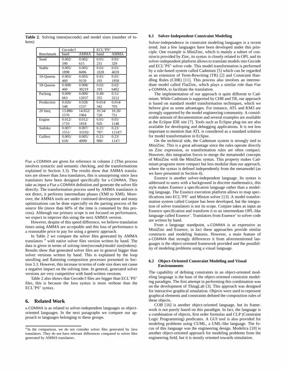
Table 2. Solving times(seconds) and model sizes (number of to-kens)
Gecode/J ECLiPSe
Benchmark hand AMMA hand AMMA
Send 0.002/ 0.002/ 0.01/ 0.01/590 615 231 329
Stable 0.005/ 0.005/ 0.01/ 0.01/1898 8496 1028 4659
10-Queens 0.003/ 0.003/ 0.01/ 0.01/460 9159 193 1958
18-Queens 0.008/ 0.008/ 0.02/ 0.02/460 30219 193 6402
Packing 0.009/ 0.009/ 0.49/ 0.51/663 12037 355 3212
Production 0.026/ 0.028/ 0.014/ 0.014/548 1537 342 703
20 Ineq 13.886/ 14.652/ 10.34/ 10.26/1576 1964 720 751
Engine 0.012/ 0.012/ 0.01/ 0.01/1710 1818 920 1148
Sudoku 0.007/ 0.007/ 0.21/ 0.23/1551/ 33192/ 797/ 11147/
Golfers 0.005/ 0.005/ 0.21/ 0.23/618/ 4098/ 980/ 1147/
Flat s-COMMA are given for reference in column 2 (This processinvolves syntactic and semantic checking, and the transformationsexplained in Section 3.3). The results show that AMMA transla-tors are slower than Java translators, this is unsurprisingsince Javatranslators have been designed specifically fors-COMMA. Theytake as input aFlat s-COMMA definition and generate the solver filedirectly. The transformation process used by AMMA translators isnot direct, it performs intermediate phases (XMI to XMI). More-over, the AMMA tools are under continued development and manyoptimizations can be done especially on the parsing processof thesource file (more than 60% of the time is consumed by this pro-cess). Although our primary scope is not focused on performance,we expect to improve this using the next AMMA version.
However, despite of this speed difference, we believe translationtimes using AMMA are acceptable and this loss of performanceisa reasonable price to pay for using a generic approach.
In Table 2 we compare the solver files generated by AMMAtranslators4 with native solver files version written by hand. Thedata is given in terms ofsolving time(seconds)/model size(tokens).Results show that generated solver files are in general bigger thansolver versions written by hand. This is explained by the loopunrolling and flattening composition processes presented in Sec-tion 3.3. However, this increase in terms of code size does not causea negative impact on the solving time. In general, generatedsolverversions are very competitive with hand-written versions.
Table 2 also shows that Gecode/J files are bigger than ECLiPSe
files, this is because the Java syntax is more verbose than theECLiPSe syntax.
6. Related Works-COMMA is as related to solver-independent languages as object-oriented languages. In the next paragraphs we compare our ap-proach to languages belonging to these groups.
4 In the comparison, we do not consider solver files generated by Javatranslators. They do not have relevant differences compared to solver filesgenerated by AMMA translators.
6.1 Solver-Independent Constraint Modeling
Solver-independence in constraint modeling languages is arecenttrend. Just a few languages have been developed under this prin-ciple. One example is MiniZinc, which is mainly a subset of con-structs provided by Zinc, its syntax is closely related to OPL and itssolver-independent platform allows to translate models into Gecodeand ECLiPSe solver code. This model transformation is performedby a rule-based system called Cadmium [5] which can be regardedas an extension of Term-Rewriting (TR) [2] and Constraint Han-dling Rules (CHR) [11]. This process also involves an interme-diate model called FlatZinc, which plays a similar role thanFlat
s-COMMA, to facilitate the translation.The implementation of our approach is quite different to Cad-
mium. While Cadmium is supported by CHR and TR, our approachis based on standard model transformation techniques, which webelieve give us some advantages. For instance, ATL and KM3 arestrongly supported by the model engineering community. A consid-erable amount of documentation and several examples are availableat the Eclipse IDE site [7]. Tools such as Eclipse plug-ins are alsoavailable for developing and debugging applications. It isnot lessimportant to mention that ATL is considered as a standard solutionfor model transformation in Eclipse.
On the technical side, the Cadmium system is strongly tied toMiniZinc. This is a great advantage since the rules operate directlyon Zinc expression, so transformation rules are often compact.However, this integration forces to merge the metamodel conceptsof MiniZinc with the MiniZinc syntax. This property makes Cad-mium programs more compact but less modular than our approach,where the syntax is defined independently from the metamodel(aswe have presented in Section 4).
Essence is another solver-independent language. Its syntax isaddressed to users with a background in discrete mathematics, thisstyle makes Essence a specification language rather than a model-ing language. The Essence execution platform allows to map spec-ifications into ECLiPSe and Minion solver [13]. A model transfor-mation system called Conjure has been developed, but the integra-tion of solver translators is not its scope. Conjure takes asinput anEssence specification and transform it to an intermediate OPL-likelanguage called Essence’. Translators from Essence’ to solver codeare written by hand.
From a language standpoint,s-COMMA is as expressive asMiniZinc and Essence, in fact these approaches provide similarconstructs and modeling features. However, a main feature ofs-COMMA that strongly differences it from aforementioned lan-guages is the object-oriented framework provided and the possibil-ity of modeling problems using a visual language.
6.2 Object-Oriented Constraint Modeling and VisualEnvironments
The capability of defining constraints in an object-oriented mod-eling language is the base of the object-oriented constraint model-ing paradigm. The first attempt in performing this combination wason the development of ThingLab [3]. This approach was designedfor interactive graphical simulation. Objects were used torepresentgraphical elements and constraints defined the compositionrules ofthese objects.
COB [16] is another object-oriented language, but its frame-work is not purely based on this paradigm. In fact, the language isa combination of objects, first order formulas and CLP (ConstraintLogic Programming) predicates. A GUI tool is also provided formodeling problems using CUML, a UML-like language. The fo-cus of this language was the engineering design. Modelica [10] isanother object-oriented approach for modeling problems from theengineering field, but it is mostly oriented towards simulation.

Gianna [25] is a precursor visual environment for modelingCSP. But its modeling style is not object-oriented and the level ofabstraction provided is lower than in UML-like languages. In thistool, CSPs are stated as constraint graphs where nodes representthe variables and the edges represent the constraints.
Although these approaches do not have a system to plug-in newsolvers and were developed for a specific application domain, webelieve it is important to mention them.
It is important to clarify too, that object-oriented capabilitiesare also provided by languages such as CoJava [4]; and in librariessuch as Gecode or ILOG SOLVER. The main difference here is thatthe host language provided is a programming language but notahigh-level modeling language. As we have explained in Section 1,advanced programming skills may be required to deal with thesetools.
7. Conclusions and Future WorkIn this work we have presenteds-COMMA, an extensible MDDplatform for modeling CSPs. The whole system is composed bytwo main parts: A modeling tool and a mapping tool, which provideto the users the following three important facilities:
• A visual modeling language that combines the declarative as-pects of constraint programming with the useful features ofobject-oriented languages. The user can state modular modelsin an intuitive way, where the compositional structure of theproblem can be easily maintained through the use of objectsunder constraints.
• Models are stated independently from solver languages. Usersare able to design just one model and to target different solvers.This clearly facilitates experimentation and benchmarking.
• A model transformation system supported by the AMMA plat-form which follows the standards of the software engineeringfield. The system allows users to plug-in new solvers withoutwriting translators by hand.
Currently, we do not uses-COMMA as our source model, be-cause its metamodel is quite large and defining generic mappings todifferent solver metamodels will be a serious challenge. Howeverwe believe that this task will lead to an interesting future work,for instance to perform reverse engineering (e.g. Gecode/Jto s-
COMMA or ECLiPSe to s-COMMA). The use of AMMA for modeloptimization will be useful too, for instance to eliminate redundantor useless constraints. The definition of selective mappings is alsoan interesting task, for instance to decide, depending on the solverused, whether loops must be unrolled or the composition mustbeflattened.
AcknowledgmentsWe are grateful to the support of this research from the “Pontifi-cia Universidad Catolica de Valparaıso” under the grant “Beca deEstudios Basica”, and to Frederic Jouault for his support on theimplementation of the AMMA translators.
References[1] ANTLR Reference Manual, 2007. http://www.antlr.org.
[2] F. Baader and T. Nipkow. Term rewriting and all that, Cambridge Univ.Press, 1998.
[3] A. Borning. The Programming Languages Aspects of ThingLab,a Constraint-Oriented Simulation Laboratory.ACM Transactions onProgramming Languages and Systems (ACM TOPLAS),3(4), pages353–387, 1981.
[4] A. Brodsky and H. Nash. CoJava: Optimization Modeling byNondeterministic Simulation. InProceedings of the 12th International
Conference on Principles and Practice of Constraint Programming (CP2006)3(4). LNCS, vol. 4204, pages 91–106, 2006.
[5] S. Brand, G. J. Duck, J. Puchinger and P. J. Stuckey. Flexible, Rule-Based Constraint Model Linearisation. InProceedings of the 10thSymposium on Practical Aspects of Declarative Languages (PADL2008). LNCS, vol. 4902, pages 68–83, 2008.
[6] D. Diaz and P. Codognet. The GNU Prolog System and its Imple-mentation. InProceedings of the 2000 ACM Symposium on AppliedComputing (SAC 2000), pages 728–732, 2000.
[7] Eclipse Model-to-model transformation, 2008.http://www.eclipse.org/m2m/.
[8] A. M. Frisch, C. Jefferson, B. Martınez Hernandez and I. Miguel. TheRules of Constraint Modelling. InProceedings of the 19th InternationalJoint Conference on Artificial Intelligence (IJCAI 2005), pages 109–116,2005.
[9] A. M. Frisch, M. Grum, C. Jefferson, B. Martınez Hernandez andI. Miguel. The Design of ESSENCE: A Constraint Language forSpecifying Combinatorial Problems. InProceedings of the 20thInternational Joint Conference on Artificial Intelligence(IJCAI 2007),pages 80–87, 2007.
[10] P. Fritzson and V. Engelson. Modelica – A Unified Object-OrientedLanguage for System Modeling and Simulation. InProceedings of the12th European Conference on Object-Oriented Programming (ECOOP1998). LNCS, vol. 1445, pages 67–90, 1998.
[11] T. W. Fruhwirth. Theory and Practice of Constraint Handling Rules.Journal of Logic Programming37(1-3), pages 95–138, 1998.
[12] Gecode System, 2006. http://www.gecode.org.
[13] I. P. Gent, C. Jefferson and I. Miguel. Minion: A Fast ScalableConstraint Solver. InProceedings of the 17th European Conference onArtificial Intelligence (ECAI 2006), pages 98–102, 2006.
[14] L. Granvilliers and F. Benhamou. Algorithm 852: RealPaver:an interval solver using constraint satisfaction techniques. ACMTransactions on Mathematical Software (ACM TOMS),32(1), pages138–156, 2006.
[15] J. Jaffar and J.-L. Lassez. Constraint Logic Programming. InProceedings of the 14th Annual ACM Symposium on Principles ofProgramming Languages (POPL 1987), pages 111–119, 1987.
[16] B. Jayaraman and P. Tambay. Modeling Engineering Structures withConstrained Objects. InProceedings of the 4th Symposium on PracticalAspects of Declarative Languages (PADL 2002). LNCS, vol. 2257,pages 28–46, 2002.
[17] F. Jouault and I. Kurtev. Transforming Models with ATL.InProceedings of Satellite Events at the 8th International Conference onModel Driven Engineering Languages and Systems (MoDELS SatelliteEvents 2005). LNCS, vol. 3844, pages 128–138, 2005.
[18] F. Jouault and J. Bezivin. KM3: A DSL for Metamodel Specification.In Proceedings of the 8th IFIP WG 6.1 International ConferenceonFormal Methods for Open Object-Based Distributed Systems (FMOODS2006). LNCS, vol. 4037, pages 171–185, 2006.
[19] F. Jouault, J. Bezivin and I. Kurtev KM3: A DSL for MetamodelSpecification. InProceedings of the 5th International Conference onGenerative Programming and Component Engineering (GPCE 2006),pages 249–254, 2006.
[20] I. Kurtev, J. Bezivin, F. Jouault and P. Valduriez. Model-basedDSL frameworks. InProceedings of Companion to the 21th AnnualACM SIGPLAN Conference on Object-Oriented Programming, Systems,Languages, and Applications (OOPSLA Companion 2006), pages 602–616, 2006.
[21] N. Nethercote, P. J. Stuckey, R. Becket, S. Brand, G. J. Duck andG. Tack. MiniZinc: Towards a Standard CP Modelling Language. InProceedings of the 13th International Conference on Principles andPractice of Constraint Programming (CP 2007)3(4). LNCS, vol. 4741,pages 529–543, 2007.
[22] OMG - Object Constraint Language (OCL) 2.0, 2006.

http://www.omg.org/cgi-bin/doc?formal/2006-05-01
[23] OMG - The Unified Modeling Language (UML) 2.1.1 InfrastructureSpecification, 2007. http://www.omg.org/spec/UML/2.1.2/.
[24] OMG - Model Driven Architecture (MDA) Guide V1.0.1, 2003http://www.omg.org/cgi-bin/doc?omg/03-06-01.
[25] M. Paltrinieri. A Visual Constraint-Programming Environment. InProceedings of the 1st International Conference on Principles andPractice of Constraint Programming (CP 1995)3(4). LNCS, vol. 976,pages 499–514, 1995.
[26] J.-F. Puget. A C++ implementation of CLP. InProceedings of theSecond Singapore International Conference on IntelligentSystems (SCIS1994), 1994.
[27] R. Rafeh, M. J. Garcıa de la Banda, K. Marriott and M. Wallace.From Zinc to Design Model. InProceedings of the 9th Symposium onPractical Aspects of Declarative Languages (PADL 2007). LNCS, vol.4354, pages 215–229, 2007.
[28] s-COMMA System, 2008. http://www.inf.ucv.cl/∼rsoto/s-comma.
[29] R. Soto and L. Granvilliers. The Design of COMMA: An ExtensibleFramework for Mapping Constrained Objects to Native SolverModels.In Proceedings of the 19th IEEE International Conference on Tools withArtificial Intelligence (ICTAI 2007), pages 243–250, 2007.
[30] P. Van Hentenryck. The OPL Language. MIT Press, 1999.
[31] M. Wallace, S. Novello and J. Schimpf. Technical report, IC-Parc,Imperial College, London, 1997.