A Simple and Efficient Boolean Solver for ConstraintLogic Programming

Philippe Codognet and Daniel DiazINRIA-RocquencourtDomaine de Voluceau BP 10578153 Le Chesnay CedexFRANCE{Philippe.Codognet, Daniel.Diaz}@inria.fr

Abstract

We study in this paper the use of consistency techniques and local propagation meth-ods, originally developped for constraints over finite domains, for solving booleanconstraints in Constraint Logic Programming (CLP). We present a boolean CLPlanguage clp(B/FD) built upon a CLP language over finite domains clp(FD) whichuses a propagation-based constraint solver. It is based on a single primitive con-straint which allows the boolean solver to be encoded at a low-level. The booleansolver obtained in this way is both very simple and very efficient: on average itis eight times faster than the CHIP propagation-based boolean solver, i.e. nearlyan order of magnitude faster, and infinitely better than the CHIP boolean unifica-tion solver. It also performs on average several times faster than special-purposestand-alone boolean solvers. We further present several simplifications of the aboveapproach, leading to the design of a very simple and compact dedicated booleansolver. This solver can be implemented in a WAM-based logical engine with aminimal extension limited to four new abstract instructions. This clp(B) systemprovides a further factor two speedup w.r.t. clp(B/FD).

1 Introduction

Constraint Logic Programming combines both the declarativity of Logic Program-ming and the ability to reason and compute with partial information (constraints)on specific domains, thus opening up a wide range of applications. Among the usualdomains found in CLP, the most widely investigated are certainly finite domains,real/rationals with arithmetic constraints, and booleans. This is exemplified bythe three main CLP languages: CHIP [31], which proposes finite domains, ratio-nal and booleans, PrologIII [11] which includes rationals, booleans and lists, andCLP(R) [18] which handles contraints over reals. Whereas most researchers agreeon the basic algorithms used in the constraint solvers for reals/rationals (simplexand gaussian elimination) and finite domains (local propagation and consistencytechniques), there are many different approaches proposed for boolean constraintsolving. Some of these solvers provide special-purpose boolean solvers while othershave been integrated inside a CLP framework. However, different algorithms havedifferent performances, and it is hard to know if, for some particular application,any specific solver will be able to solve it in practise. Obviously, the well-knownNP-completeness of the satisfiability of boolean formulas shows that we are tackling

1

a difficult problem here.Over recent years, local propagation methods, developed in the CHIP language forfinite domain constraints [31], have gained a great success for many applications,including real-life industrial problems. They stem from consistency techniques in-troduced in AI for Constraint Satisfaction Problems (CSP) [19]. Such techniqueshave also been used in CHIP to solve boolean constraints with some success; infact to such an extent that it has become the standard tool in the commercial ver-sion of CHIP. This method performs better than the original boolean unificationalgorithm for nearly all problems and is competitive with special-purpose booleansolvers. Thus, the basic idea is that an efficient boolean solver can be derived froma finite domain constraint solver for free.It was therefore quite natural to investigate such a possiblity with our CLP systemclp(FD), which handles finite domains constraints similar to that of CHIP, butbeing nevertheless about four times faster on average [13, 10]. clp(FD) is basedon the so-called “glass-box” approach proposed by [32], as opposed to the “black-box” approach of the CHIP solver for instance. The basic idea is to have a singleconstraint X in r, where r denotes a range (e.g. t1..t2). More complex constraintssuch as linear equations and inequations are then defined in terms of this primitiveconstraint. The X in r constraint can be seen as embedding the core propagationmechanism for constraint solving over finite domains, and can be seen as an abstractmachine for propagation-based constraint solving.We can therefore directly encode a boolean solver at a low-level with this basicmechanism, and decompose boolean constraints such as and, or, and not in X in rexpressions. In this way, we obtain a boolean solver which is obviously more efficientthan the encoding of booleans with arithmetic constraints or with the less adequateprimitives of CHIP. Worth noticing is that this boolean extension, called clp(B/FD),is very simple; the overall solver (coding of boolean constraints in X in r expression)being about ten lines long, the glass-box is very clear indeed... Moreover, thissolver is surprisingly very efficient, being eight times faster on average than theCHIP solver (reckoned to be efficient), with peak speedup reaching two orders ofmagnitude in some cases. clp(B/FD) is also more efficient than special purposesolvers, such as solvers based on Binary Decision Diagrams (BDDs), enumerativemethods or schemes using techniques borrowed from Operational Research. Thisarchitecture also has several other advantages, as follows. First, being integratedin a full CLP language, heuristics can be added in the program itself, as opposedto a closed boolean solver with (a finite set of) built-in heuristics. Second, beingintegrated in a finite domain solver, various extensions such as pseudo-booleans [6]or multi-valued logics [33] can be integrated straightforwardly. Third, being basedon a propagation method, searching for a single solution can be done much morequickly if the computation of all solutions is not needed.Nevertheless, performances can be improved by simplifying the data-structures usedin clp(FD), which are indeed designed for full finite domain constraints. They canbe specialized by introducing explicitly a new type and new instructions for booleanvariables. It is possible, for instance, to reduce the data-structure representing thedomain of a variable and its associated constraints to only two words: one pointingto the chain of constraints to awake when the variable is bound to 0 and the otherwhen it is bound to 1. Also some other data-structures become useless for booleanvariables, and can be simplified. Such a solver is very compact and simple; it isbased again on the glass-box approach, and uses only a single low-level constraint,more specialized than the X in r construct, into which boolean constraints suchas and, or or not are decomposed. This primitive constraint can be implemented

2

into a WAM-based logical engine with a minimal extension : only four new abstractinstructions are needed. This dedicated solver, called clp(B), provides a furtherfactor two speedup w.r.t. clp(B/FD).

The rest of this paper is organized as follows. Section 2 reviews the variety ofmethods already proposed for solving boolean constraints and presents in particularthe use of local propagation and consistency techniques. Section 3 introduces theformalization of the semantics of propagation-based boolean solvers as a particularconstraint system. Section 4 then proposes a first implementation on top of theclp(FD) system by using the X in r primitive constraint for decomposing booleanconstraints. The performances of this system, called clp(B/FD), are evaluatedin section 5, and compared both with the CHIP system and with several otherefficient dedicated boolean solvers. In section 6, a number of simplifications of theprevious approach are proposed, leading to the design of a very simple and compactspecialized boolean solver, called clp(B), performances of which are detailed insection 7. A short conclusion and research perspectives end the paper.

2 A review of Boolean solvers

Although the problem of satisfiability of a set of boolean formulas is quite old,designing efficient methods is still an active area of research, and there has beena variety of methods proposed over recent years toward this aim. Moreover, it isusually important not only to test for satisfiability but also to actually compute themodels (assignments of variables), if any. To do so, several types of methods havebeen developed, based on very different data-structures and algorithms. Focusing onimplemented systems, existing boolean solvers can be roughly classified as follows.

2.1 Resolution-based methods

The resolution method, which has been proposed for full first-order logic, can obvi-ously be specialized for propositional logic and therefore be used for solving booleanproblems. Such a method is based on clausal representation for boolean formulas,each literal representing a boolean variable, i.e. conjunctive normal form. The coreof the method will consist in trying to apply resolution steps between clauses con-taining occurences of the same variable with opposite signs until either the emptyclause (inconsistency) is derived, or some desired consequence of the original formu-las is derived. SL-resolution is for instance used for solving boolean constraints inthe current version of the Prolog-III language [11] [2]. However, the performancesof this solver are very poor and limit its use to small problems. Many refinementshave been proposed for limiting the potentially huge search space that have to beexplored in resolution-based methods, see [24] for a detailed discussion and furtherreferences. Another improved resolution-based algorithm, using a relaxation proce-dure, is described in [15]. However, there does not seem to be any general solutionwhich can improve efficiency for a large class of problems.

2.2 BDD-based methods

Binary Decision Diagrams (BDD) have recently gained great success as an efficientway to encode boolean functions [7], and it was natural to try to use them in booleansolvers. The basic idea of BDDs is to have a compact representation of the Shanon

3

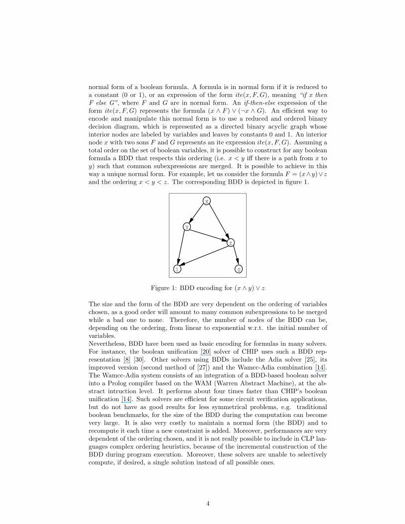
normal form of a boolean formula. A formula is in normal form if it is reduced toa constant (0 or 1), or an expression of the form ite(x, F,G), meaning “if x thenF else G”, where F and G are in normal form. An if-then-else expression of theform ite(x, F,G) represents the formula (x ∧ F ) ∨ (¬x ∧ G). An efficient way toencode and manipulate this normal form is to use a reduced and ordered binarydecision diagram, which is represented as a directed binary acyclic graph whoseinterior nodes are labeled by variables and leaves by constants 0 and 1. An interiornode x with two sons F and G represents an ite expression ite(x, F,G). Assuming atotal order on the set of boolean variables, it is possible to construct for any booleanformula a BDD that respects this ordering (i.e. x < y iff there is a path from x toy) such that common subexpressions are merged. It is possible to achieve in thisway a unique normal form. For example, let us consider the formula F = (x∧y)∨zand the ordering x < y < z. The corresponding BDD is depicted in figure 1.

X

Y

Z

1 0

Figure 1: BDD encoding for (x ∧ y) ∨ z

The size and the form of the BDD are very dependent on the ordering of variableschosen, as a good order will amount to many common subexpressions to be mergedwhile a bad one to none. Therefore, the number of nodes of the BDD can be,depending on the ordering, from linear to exponential w.r.t. the initial number ofvariables.Nevertheless, BDD have been used as basic encoding for formulas in many solvers.For instance, the boolean unification [20] solver of CHIP uses such a BDD rep-resentation [8] [30]. Other solvers using BDDs include the Adia solver [25], itsimproved version (second method of [27]) and the Wamcc-Adia combination [14].The Wamcc-Adia system consists of an integration of a BDD-based boolean solverinto a Prolog compiler based on the WAM (Warren Abstract Machine), at the ab-stract intruction level. It performs about four times faster than CHIP’s booleanunification [14]. Such solvers are efficient for some circuit verification applications,but do not have as good results for less symmetrical problems, e.g. traditionalboolean benchmarks, for the size of the BDD during the computation can becomevery large. It is also very costly to maintain a normal form (the BDD) and torecompute it each time a new constraint is added. Moreover, performances are verydependent of the ordering chosen, and it is not really possible to include in CLP lan-guages complex ordering heuristics, because of the incremental construction of theBDD during program execution. Moreover, these solvers are unable to selectivelycompute, if desired, a single solution instead of all possible ones.

4

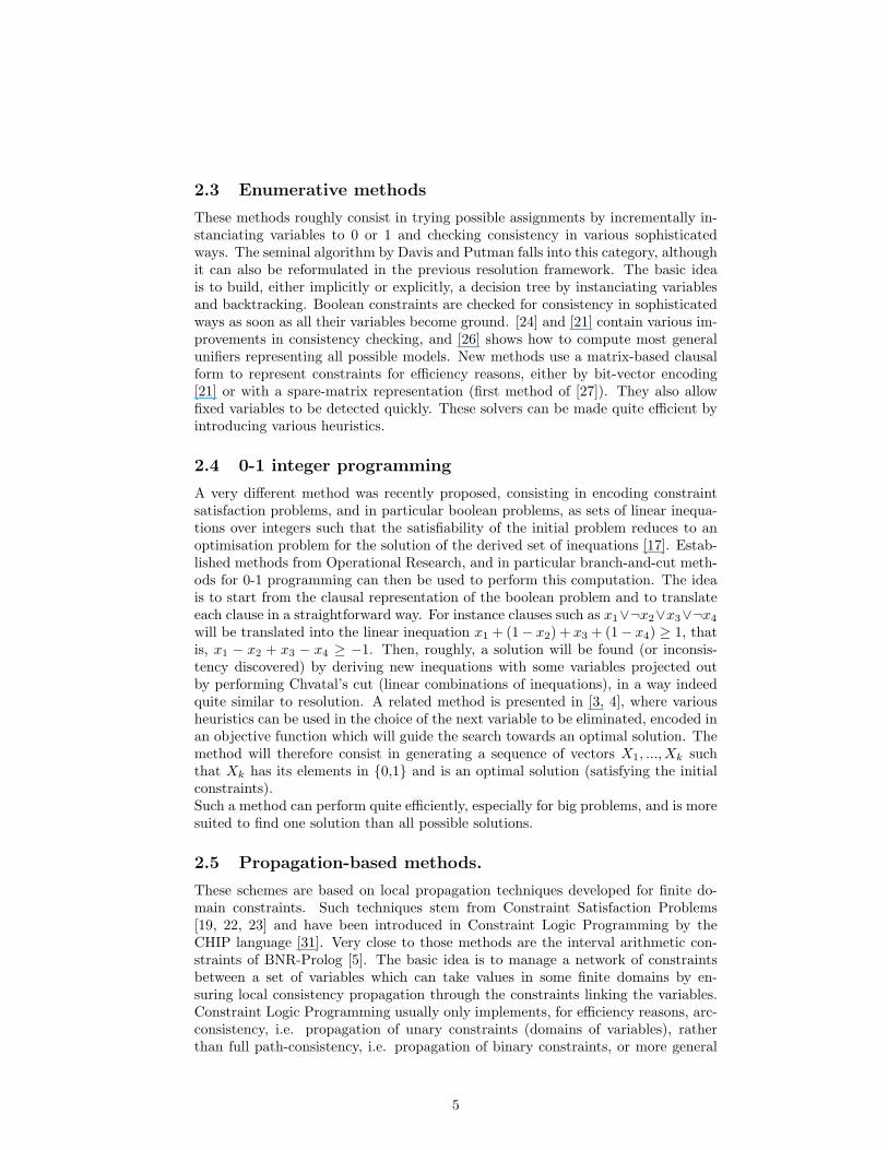
2.3 Enumerative methods

These methods roughly consist in trying possible assignments by incrementally in-stanciating variables to 0 or 1 and checking consistency in various sophisticatedways. The seminal algorithm by Davis and Putman falls into this category, althoughit can also be reformulated in the previous resolution framework. The basic ideais to build, either implicitly or explicitly, a decision tree by instanciating variablesand backtracking. Boolean constraints are checked for consistency in sophisticatedways as soon as all their variables become ground. [24] and [21] contain various im-provements in consistency checking, and [26] shows how to compute most generalunifiers representing all possible models. New methods use a matrix-based clausalform to represent constraints for efficiency reasons, either by bit-vector encoding[21] or with a spare-matrix representation (first method of [27]). They also allowfixed variables to be detected quickly. These solvers can be made quite efficient byintroducing various heuristics.

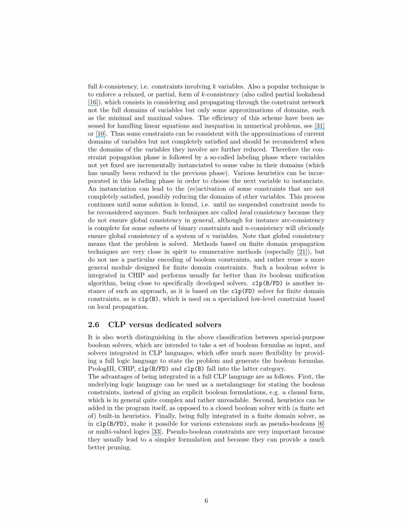
2.4 0-1 integer programming

A very different method was recently proposed, consisting in encoding constraintsatisfaction problems, and in particular boolean problems, as sets of linear inequa-tions over integers such that the satisfiability of the initial problem reduces to anoptimisation problem for the solution of the derived set of inequations [17]. Estab-lished methods from Operational Research, and in particular branch-and-cut meth-ods for 0-1 programming can then be used to perform this computation. The ideais to start from the clausal representation of the boolean problem and to translateeach clause in a straightforward way. For instance clauses such as x1∨¬x2∨x3∨¬x4

will be translated into the linear inequation x1 + (1− x2) + x3 + (1− x4) ≥ 1, thatis, x1 − x2 + x3 − x4 ≥ −1. Then, roughly, a solution will be found (or inconsis-tency discovered) by deriving new inequations with some variables projected outby performing Chvatal’s cut (linear combinations of inequations), in a way indeedquite similar to resolution. A related method is presented in [3, 4], where variousheuristics can be used in the choice of the next variable to be eliminated, encoded inan objective function which will guide the search towards an optimal solution. Themethod will therefore consist in generating a sequence of vectors X1, ..., Xk suchthat Xk has its elements in {0,1} and is an optimal solution (satisfying the initialconstraints).Such a method can perform quite efficiently, especially for big problems, and is moresuited to find one solution than all possible solutions.

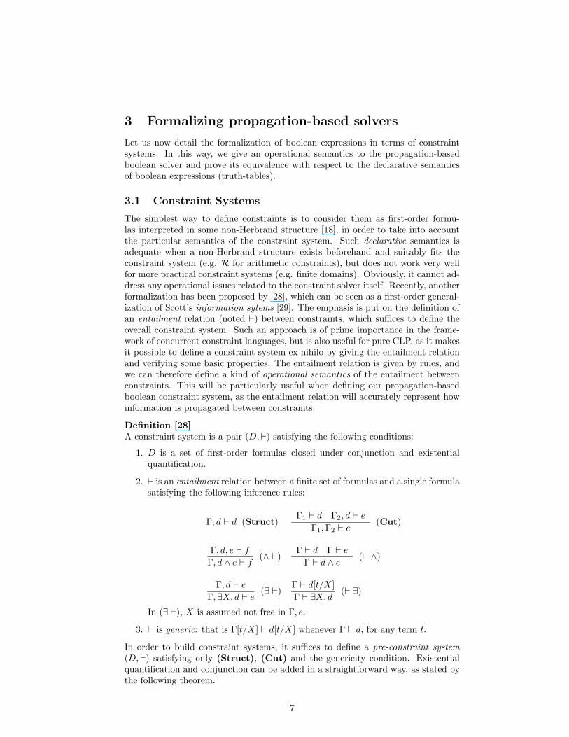
2.5 Propagation-based methods.

These schemes are based on local propagation techniques developed for finite do-main constraints. Such techniques stem from Constraint Satisfaction Problems[19, 22, 23] and have been introduced in Constraint Logic Programming by theCHIP language [31]. Very close to those methods are the interval arithmetic con-straints of BNR-Prolog [5]. The basic idea is to manage a network of constraintsbetween a set of variables which can take values in some finite domains by en-suring local consistency propagation through the constraints linking the variables.Constraint Logic Programming usually only implements, for efficiency reasons, arc-consistency, i.e. propagation of unary constraints (domains of variables), ratherthan full path-consistency, i.e. propagation of binary constraints, or more general

5

full k-consistency, i.e. constraints involving k variables. Also a popular technique isto enforce a relaxed, or partial, form of k-consistency (also called partial lookahead[16]), which consists in considering and propagating through the constraint networknot the full domains of variables but only some approximations of domains, suchas the minimal and maximal values. The efficiency of this scheme have been as-sessed for handling linear equations and inequation in numerical problems, see [31]or [10]. Thus some constraints can be consistent with the approximations of currentdomains of variables but not completely satisfied and should be reconsidered whenthe domains of the variables they involve are further reduced. Therefore the con-straint popagation phase is followed by a so-called labeling phase where variablesnot yet fixed are incrementally instanciated to some value in their domains (whichhas usually been reduced in the previous phase). Various heuristics can be incor-porated in this labeling phase in order to choose the next variable to instanciate.An instanciation can lead to the (re)activation of some constraints that are notcompletely satisfied, possibly reducing the domains of other variables. This processcontinues until some solution is found, i.e. until no suspended constraint needs tobe reconsidered anymore. Such techniques are called local consistency because theydo not ensure global consistency in general, although for instance arc-consistencyis complete for some subsets of binary constraints and n-consistency will obviouslyensure global consistency of a system of n variables. Note that global consistencymeans that the problem is solved. Methods based on finite domain propagationtechniques are very close in spirit to enumerative methods (especially [21]), butdo not use a particular encoding of boolean constraints, and rather reuse a moregeneral module designed for finite domain constraints. Such a boolean solver isintegrated in CHIP and performs usually far better than its boolean unificationalgorithm, being close to specifically developed solvers. clp(B/FD) is another in-stance of such an approach, as it is based on the clp(FD) solver for finite domainconstraints, as is clp(B), which is used on a specialized low-level constraint basedon local propagation.

2.6 CLP versus dedicated solvers

It is also worth distinguishing in the above classification between special-purposeboolean solvers, which are intended to take a set of boolean formulas as input, andsolvers integrated in CLP languages, which offer much more flexibility by provid-ing a full logic language to state the problem and generate the boolean formulas.PrologIII, CHIP, clp(B/FD) and clp(B) fall into the latter category.The advantages of being integrated in a full CLP language are as follows. First, theunderlying logic language can be used as a metalanguage for stating the booleanconstraints, instead of giving an explicit boolean formulations, e.g. a clausal form,which is in general quite complex and rather unreadable. Second, heuristics can beadded in the program itself, as opposed to a closed boolean solver with (a finite setof) built-in heuristics. Finally, being fully integrated in a finite domain solver, asin clp(B/FD), make it possible for various extensions such as pseudo-booleans [6]or multi-valued logics [33]. Pseudo-boolean constraints are very important becausethey usually lead to a simpler formulation and because they can provide a muchbetter pruning.

6

3 Formalizing propagation-based solvers

Let us now detail the formalization of boolean expressions in terms of constraintsystems. In this way, we give an operational semantics to the propagation-basedboolean solver and prove its equivalence with respect to the declarative semanticsof boolean expressions (truth-tables).

3.1 Constraint Systems

The simplest way to define constraints is to consider them as first-order formu-las interpreted in some non-Herbrand structure [18], in order to take into accountthe particular semantics of the constraint system. Such declarative semantics isadequate when a non-Herbrand structure exists beforehand and suitably fits theconstraint system (e.g. R for arithmetic constraints), but does not work very wellfor more practical constraint systems (e.g. finite domains). Obviously, it cannot ad-dress any operational issues related to the constraint solver itself. Recently, anotherformalization has been proposed by [28], which can be seen as a first-order general-ization of Scott’s information sytems [29]. The emphasis is put on the definition ofan entailment relation (noted `) between constraints, which suffices to define theoverall constraint system. Such an approach is of prime importance in the frame-work of concurrent constraint languages, but is also useful for pure CLP, as it makesit possible to define a constraint system ex nihilo by giving the entailment relationand verifying some basic properties. The entailment relation is given by rules, andwe can therefore define a kind of operational semantics of the entailment betweenconstraints. This will be particularly useful when defining our propagation-basedboolean constraint system, as the entailment relation will accurately represent howinformation is propagated between constraints.

Definition [28]A constraint system is a pair (D,`) satisfying the following conditions:

1. D is a set of first-order formulas closed under conjunction and existentialquantification.

2. ` is an entailment relation between a finite set of formulas and a single formulasatisfying the following inference rules:

Γ, d ` d (Struct)Γ1 ` d Γ2, d ` e

Γ1,Γ2 ` e(Cut)

Γ, d, e ` f

Γ, d ∧ e ` f(∧ `)

Γ ` d Γ ` e

Γ ` d ∧ e(` ∧)

Γ, d ` e

Γ,∃X. d ` e(∃ `)

Γ ` d[t/X]Γ ` ∃X. d

(` ∃)

In (∃ `), X is assumed not free in Γ, e.

3. ` is generic: that is Γ[t/X] ` d[t/X] whenever Γ ` d, for any term t.

In order to build constraint systems, it suffices to define a pre-constraint system(D,`) satisfying only (Struct), (Cut) and the genericity condition. Existentialquantification and conjunction can be added in a straightforward way, as stated bythe following theorem.

7

Theorem [28]Let (D′,`′) be a pre-constraint system. Let D be the closure of D′ under existentialquantification and conjunction, and ` the closure of `′ under the basic inferencerules. Then (D,`) is a constraint system.

As an important corollary, a constraint system can be constructed even more simplyfrom any first-order theory, i.e. any set of first-order formulas. Consider a theory Tand take for D the closure of the subset of formulas in the vocabulary of T underexistential quantification and conjunction. Then one defines the entailment relation`T as follows. Γ `T d iff Γ entails d in the logic, with the extra non-logical axiomsof T .Then (D,`T ) can be easily verified to be a constraint system.Observe that this definition of constraint systems thus naturally encompasses thetraditional view of constraints as interpreted formulas.

3.2 Boolean constraints

DefinitionLet V be an enumerable set of variables. A boolean constraint on V is one of thefollowing formulas:

and(X, Y, Z) , or(X, Y, Z) , not(X, Y ) , X = Y , for X, Y, Z ∈ V ∪ {0, 1}

The intuitive meaning of these constraints is: X ∧ Y ≡ Z, X ∨ Y ≡ Z, X ≡ ¬Y ,and X ≡ Y . We note B the set of all such boolean constraints.

Let us now present the rules defining the propagation between boolean constraints.

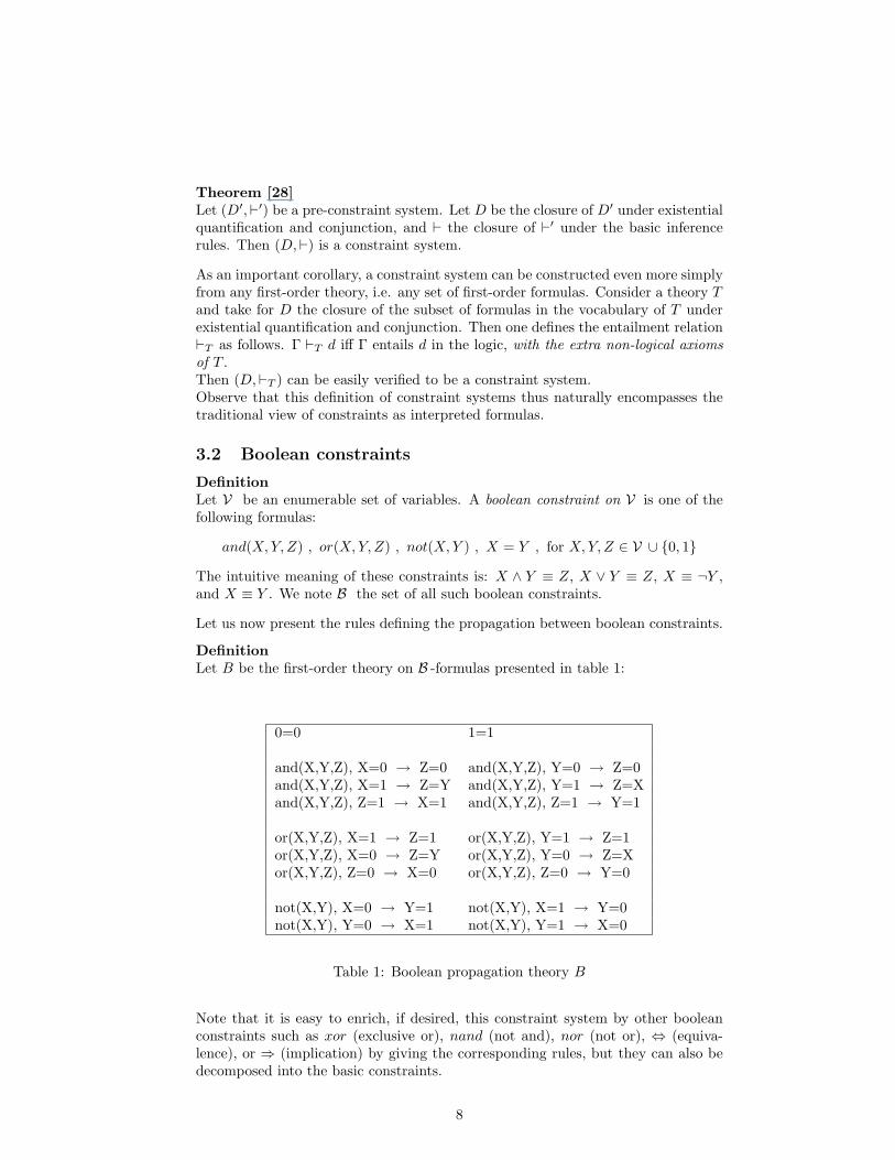
DefinitionLet B be the first-order theory on B -formulas presented in table 1:

0=0 1=1

and(X,Y,Z), X=0 → Z=0 and(X,Y,Z), Y=0 → Z=0and(X,Y,Z), X=1 → Z=Y and(X,Y,Z), Y=1 → Z=Xand(X,Y,Z), Z=1 → X=1 and(X,Y,Z), Z=1 → Y=1

or(X,Y,Z), X=1 → Z=1 or(X,Y,Z), Y=1 → Z=1or(X,Y,Z), X=0 → Z=Y or(X,Y,Z), Y=0 → Z=Xor(X,Y,Z), Z=0 → X=0 or(X,Y,Z), Z=0 → Y=0

not(X,Y), X=0 → Y=1 not(X,Y), X=1 → Y=0not(X,Y), Y=0 → X=1 not(X,Y), Y=1 → X=0

Table 1: Boolean propagation theory B

Note that it is easy to enrich, if desired, this constraint system by other booleanconstraints such as xor (exclusive or), nand (not and), nor (not or), ⇔ (equiva-lence), or ⇒ (implication) by giving the corresponding rules, but they can also bedecomposed into the basic constraints.

8

We can now define the entailment relation `B between boolean constraints and theboolean constraint system:

DefinitionsConsider a store Γ and a boolean constraint b.

Γ `B b iff Γ entails b with the extra axioms of B.

The boolean constraint system is (B ,`B).

It is worth noticing that the rules of B (and thus `B) precisely encode the propa-gation mechanisms that will be used to solve boolean constraints. We have indeedgiven the operational semantics of the constraint solver in this way.

3.3 Correctness and completeness of (B ,`B)

It is important to ensure that our (operationally-defined) constraint system is equiv-alent to traditional boolean expressions. To do so, we have to prove that our en-tailment relation derives the same results as the declarative semantics of booleansgiven by the truth-tables of the and, or and not operators.

TheoremThe and(X, Y, Z), or(X, Y, Z), and not(X, Y ) constraints are satisfied for somevalues of X, Y and Z iff the tuple of variables is given by the truth-tables of thecorresponding boolean operators.

ProofIt must be shown that, for and(X, Y, Z) and or(X, Y, Z), once X and Y are bound tosome value, the value of Z is correct, i.e. it is unique (if several rules can be applied,they give the same result) and it is equal to the value given by the correspondingtruth-table, and that all rows of the truth-tables are reached.This can be verified by a straightforward case analysis.For not(X, Y ) it can be easily shown that for any X, Y is given the opposite value.

4 Booleans on top of clp(FD)

The first approach we will present consists of implementing boolean constraints inthe constraint logic programming language over finite domains clp(FD), by usingthe possibility to define new constraints in terms of the unique primitive constraintof the system.

4.1 clp(FD) in a nutshell

As introduced in Logic Programming by the CHIP language, clp(FD) [13] is aconstraint logic language based on finite domains, where constraint solving is doneby propagation and consistency techniques originating from Constraint SatisfactionProblems [19, 23, 34]. The novelty of clp(FD) is the use of a unique primitiveconstraint which allows the user to define his own high-level constraints. The blackbox approach gives way to glass box approach.

9

4.1.1 The constraint X in r

The main idea is to use a single primitive constraint X in r, where X is a finitedomain (FD) variable and r denotes a range, which can be not only a constantrange, e.g. 1..10 but also an indexical range using:

• min(Y ) which represents the minimal value of Y (in the current store),

• max(Y ) which represents the maximal value of Y ,

• val(Y ) which represents the value of Y as soon as Y is ground.

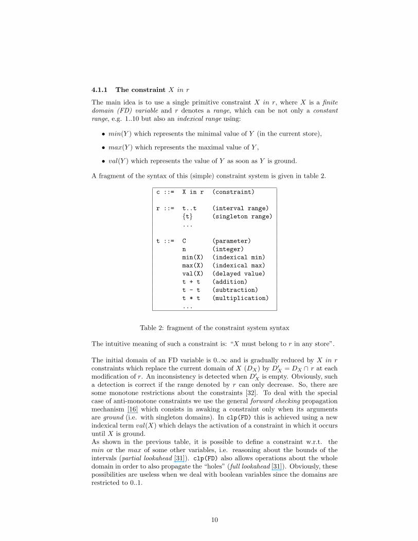
A fragment of the syntax of this (simple) constraint system is given in table 2.

c ::= X in r (constraint)

r ::= t..t (interval range){t} (singleton range)...

t ::= C (parameter)n (integer)min(X) (indexical min)max(X) (indexical max)val(X) (delayed value)t + t (addition)t - t (subtraction)t * t (multiplication)...

Table 2: fragment of the constraint system syntax

The intuitive meaning of such a constraint is: “X must belong to r in any store”.

The initial domain of an FD variable is 0..∞ and is gradually reduced by X in rconstraints which replace the current domain of X (DX) by D′

X = DX ∩ r at eachmodification of r. An inconsistency is detected when D′

X is empty. Obviously, sucha detection is correct if the range denoted by r can only decrease. So, there aresome monotone restrictions about the constraints [32]. To deal with the specialcase of anti-monotone constraints we use the general forward checking propagationmechanism [16] which consists in awaking a constraint only when its argumentsare ground (i.e. with singleton domains). In clp(FD) this is achieved using a newindexical term val(X) which delays the activation of a constraint in which it occursuntil X is ground.As shown in the previous table, it is possible to define a constraint w.r.t. themin or the max of some other variables, i.e. reasoning about the bounds of theintervals (partial lookahead [31]). clp(FD) also allows operations about the wholedomain in order to also propagate the “holes” (full lookahead [31]). Obviously, thesepossibilities are useless when we deal with boolean variables since the domains arerestricted to 0..1.

10

4.1.2 High-level constraints and propagation mechanism

From X in r constraints, it is possible to define high-level constraints (called userconstraints) as Prolog predicates. Each constraint specifies how the constrainedvariable must be updated when the domains of other variables change. In thefollowing examples X, Y are FD variables and C is a parameter (runtime constantvalue).

’x+y=c’(X,Y,C):- X in C-max(Y)..C-min(Y), (C1)Y in C-max(X)..C-min(X). (C2)

’x-y=c’(X,Y,C):- X in min(Y)+C..max(Y)+C, (C3)Y in min(X)-C..max(X)-C. (C4)

The constraint x+y=c is a classical FD constraint reasoning about intervals. Thedomain of X is defined w.r.t. the bounds of the domain of Y .

In order to show how the propagation mechanism works, let us trace the resolutionof the system {X + Y = 4, X − Y = 2} (translated via ’x+y=c’(X,Y,4) and’x-y=c’(X,Y,2)):After executing ’x+y=c’(X,Y,4), the domain of X and Y are reduced to 0..4 (C1

is in the current store: X in − ∞..4, C2 : Y in − ∞..4). And, after executing’x-y=c’(X,Y,2), the domain of X is reduced to 2..4 (C3 : X in 2..6), which thenreduces the domain of Y to 0..2 (C4 : Y in 0..2).Note that the unique solution {X = 3, Y = 1} has not yet been found. Indeed,in order to efficiently achieve consistency, the traditional method (arc-consistency)only checks that, for any constraint C involving X and Y , for each value in thedomain of X there exists a value in the domain of Y satisfying C and vice-versa.So, once arc-consistency has been achieved and the domains have been reduced, anenumeration (called labeling) has to be done on the domains of the variables to yieldthe exact solutions. Namely, X is assigned to one value in DX , its consequencesare propagated to other variables, and so on. If an inconsistency arises, othervalues for X are tried by backtracking. Note that the order used to enumerate thevariables and to generate the values for a variable can improve the efficiency in avery significant manner (see heuristics in [31]).In our example, when the value 2 is tried for X, C2 and C4 are awoken (becausethey depend on X). C2 sets Y to 2 and C4 detects the inconsistency when it triesto set Y to 0. The backtracking reconsiders X and tries value 3 and, as previously,C2 and C4 are reexecuted to set (and check) Y to 1. The solution {X = 3, Y = 1}is then obtained.

4.1.3 Optimizations

The uniform treatment of a single primitive for all complex user constraints lead toa better understanding of the overall constraint solving process and allows for (afew) global optimizations, as opposed to the many local and particular optimizationshidden inside the black-box. When a constraint X in r has been reexecuted, if D′

X =DX it was useless to reexecute it (i.e. it has neither failed nor reduced the domainof X). Hence, we have designed three simple but powerful optimizations for theX in r constraint [13, 10] which encompass many previous particular optimizationsfor FD constraints:

11

• some constraints are equivalent so only the execution of one of them is needed.In the previous example, when C2 is called in the store {X in 0..4, Y in 0..∞}Y is set to 0..4. Since the domain of Y has been updated, all constraintsdepending on Y are reexecuted and C1 (X in 0..4) is awoken unnecessarily(C1 and C2 are equivalent).

• it is useless to reexecute a constraint as soon as it is entailed. In clp(FD),only one approximation is used to detect the entailment of a constraint X in rwhich is “X is ground”. So, it is useless to reexecute a constraint X in r assoon as X is ground.

• when a constraint is awoken more than once from several distinct variables,only one reexecution is necessary. This optimization is obvious since the orderof constraints, during the execution, is irrelevant for correctness.

These optimizations make it possible to avoid on average 50 % of the total numberof constraint executions on a traditional set of FD benchmarks (see [13, 10] for fulldetails) and up to 57 % on the set of boolean benchmarks presented below.

4.1.4 Performances

Full implementation results about the performances of clp(FD) can be found in[13, 10], and show that this “glass-box” approach is sound and can be competitivein terms of efficiency with the more traditional “black-box” approach of languagessuch as CHIP. On a traditional set of benchmark programs, mostly taken from [31],the clp(FD) engine is on average about four times faster than the CHIP system,with peak speedup reaching eight.

4.2 Building clp(B/FD)

In this section we specify the constraint solver, i.e. we define a user constraint foreach boolean constraint presented above. We then prove the correctness and com-pleteness of this solver, and show how it really encodes the “operational semantics”defined by theory B.

4.2.1 Designing the constraints

The design of the solver only consists in defining a user constraint for each booleanconstraint. As the constraint X in r makes it possible to use arithmetic operationson the bounds of a domain, we use some mathematical relations satisfied by theboolean constraints:

12

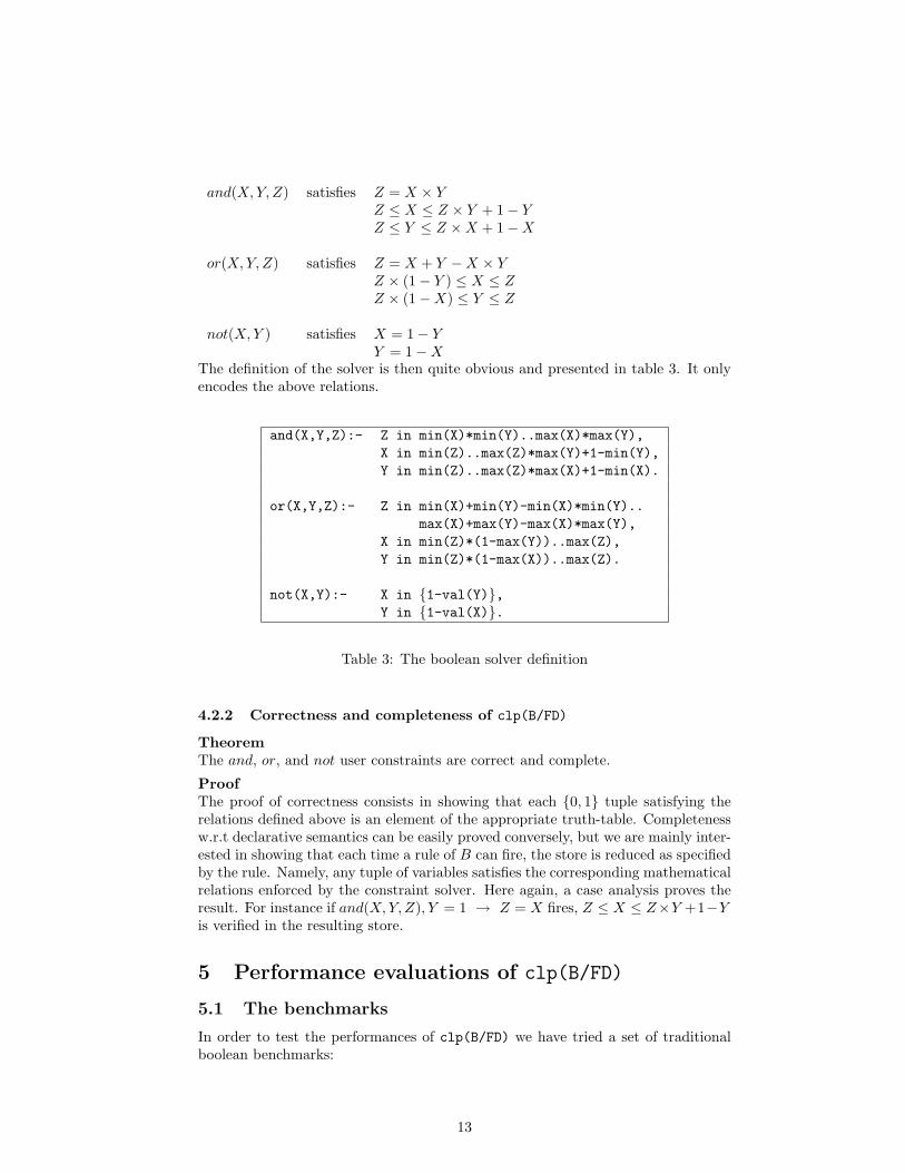
and(X, Y, Z) satisfies Z = X × YZ ≤ X ≤ Z × Y + 1− YZ ≤ Y ≤ Z ×X + 1−X

or(X, Y, Z) satisfies Z = X + Y −X × YZ × (1− Y ) ≤ X ≤ ZZ × (1−X) ≤ Y ≤ Z

not(X, Y ) satisfies X = 1− YY = 1−X

The definition of the solver is then quite obvious and presented in table 3. It onlyencodes the above relations.

and(X,Y,Z):- Z in min(X)*min(Y)..max(X)*max(Y),X in min(Z)..max(Z)*max(Y)+1-min(Y),Y in min(Z)..max(Z)*max(X)+1-min(X).

or(X,Y,Z):- Z in min(X)+min(Y)-min(X)*min(Y)..max(X)+max(Y)-max(X)*max(Y),

X in min(Z)*(1-max(Y))..max(Z),Y in min(Z)*(1-max(X))..max(Z).

not(X,Y):- X in {1-val(Y)},Y in {1-val(X)}.

Table 3: The boolean solver definition

4.2.2 Correctness and completeness of clp(B/FD)

TheoremThe and, or, and not user constraints are correct and complete.

ProofThe proof of correctness consists in showing that each {0, 1} tuple satisfying therelations defined above is an element of the appropriate truth-table. Completenessw.r.t declarative semantics can be easily proved conversely, but we are mainly inter-ested in showing that each time a rule of B can fire, the store is reduced as specifiedby the rule. Namely, any tuple of variables satisfies the corresponding mathematicalrelations enforced by the constraint solver. Here again, a case analysis proves theresult. For instance if and(X, Y, Z), Y = 1 → Z = X fires, Z ≤ X ≤ Z×Y +1−Yis verified in the resulting store.

5 Performance evaluations of clp(B/FD)

5.1 The benchmarks

In order to test the performances of clp(B/FD) we have tried a set of traditionalboolean benchmarks:

13

• schur: Schur’s lemma. The problem consists in finding a 3-coloring of theintegers {1 . . . n} such that there is no monochrome triplet (x, y, z) wherex + y = z. The formulation uses 3× n variables to indicate, for each integer,its color. This problem has a solution iff n ≤ 13.

• pigeon: the pigeon-hole problem consists in putting n pigeons in m pigeon-holes (at most 1 pigeon per hole). The boolean formulation uses n×m vari-ables to indicate, for each pigeon, its hole number. Obviously, there is asolution iff n ≤ m.

• queens: place n queens on a n× n chessboard such that there are no queensthreatening each other. The boolean formulation uses n × n variables toindicate, for each square, if there is a queen on it.

• ramsey: find a 3-coloring of a complete graph with n vertices such that thereis no monochrome triangles. The formulation uses 3 variables per edge toindicate its color. There is a solution iff n ≤ 16.

All solutions are computed unless otherwise stated. The results presented below forclp(B/FD) do not include any heuristics and have been measured on a Sun Sparc2 (28.5 Mips). The following section compares clp(B/FD) with the commercialversion of CHIP. We have chosen CHIP for the main comparison because it is acommercial product and a CLP language (and not only a constraint solver) andthus accepts the same programs as clp(B/FD). Moreover, it also uses a booleanconstraint solver based on finite domains1. We also compare clp(B/FD) with otherspecific constraint solvers.

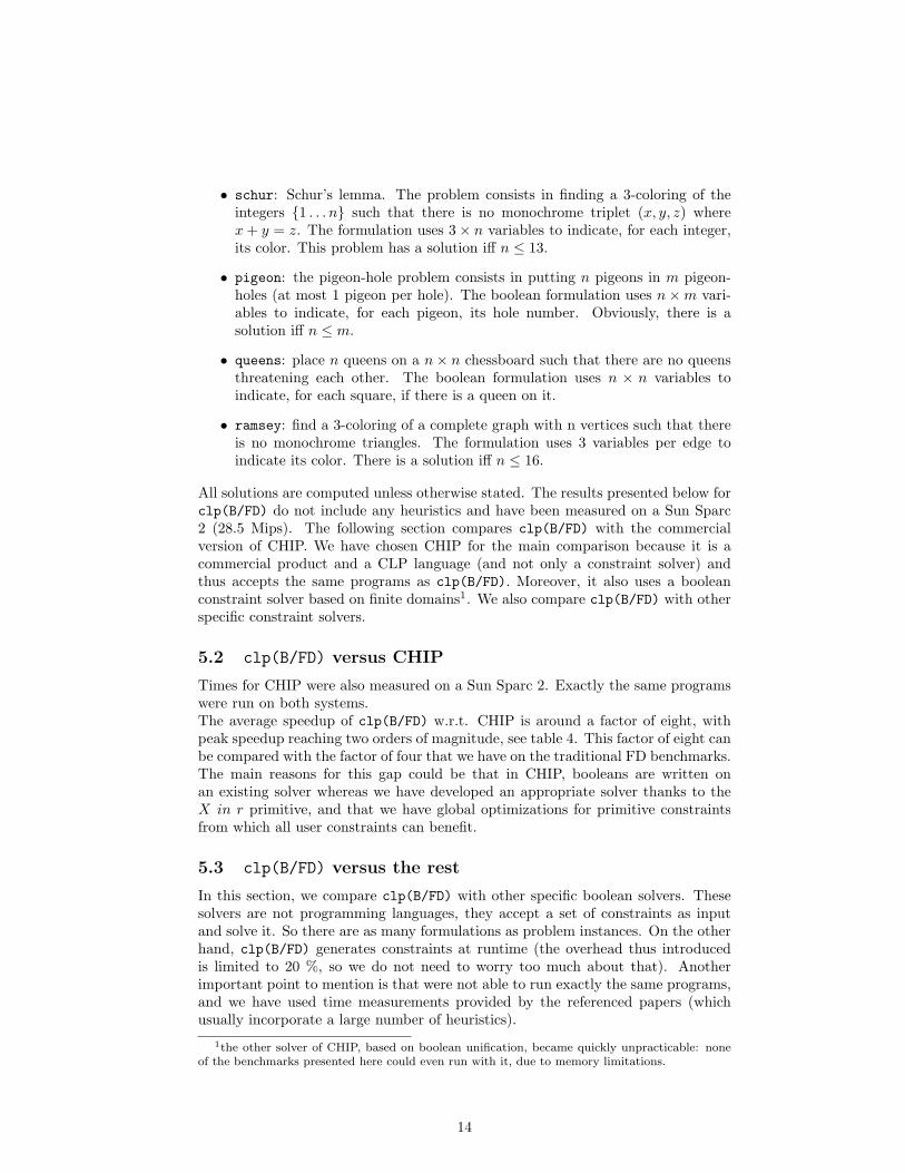
5.2 clp(B/FD) versus CHIP

Times for CHIP were also measured on a Sun Sparc 2. Exactly the same programswere run on both systems.The average speedup of clp(B/FD) w.r.t. CHIP is around a factor of eight, withpeak speedup reaching two orders of magnitude, see table 4. This factor of eight canbe compared with the factor of four that we have on the traditional FD benchmarks.The main reasons for this gap could be that in CHIP, booleans are written onan existing solver whereas we have developed an appropriate solver thanks to theX in r primitive, and that we have global optimizations for primitive constraintsfrom which all user constraints can benefit.

5.3 clp(B/FD) versus the rest

In this section, we compare clp(B/FD) with other specific boolean solvers. Thesesolvers are not programming languages, they accept a set of constraints as inputand solve it. So there are as many formulations as problem instances. On the otherhand, clp(B/FD) generates constraints at runtime (the overhead thus introducedis limited to 20 %, so we do not need to worry too much about that). Anotherimportant point to mention is that were not able to run exactly the same programs,and we have used time measurements provided by the referenced papers (whichusually incorporate a large number of heuristics).

1the other solver of CHIP, based on boolean unification, became quickly unpracticable: noneof the benchmarks presented here could even run with it, due to memory limitations.

14

CHIP clp(B/FD) CHIPProgram Time (s) Time (s) clp(B/FD)schur 13 0.830 0.100 8.30schur 14 0.880 0.100 8.80schur 30 9.370 0.250 37.48schur 100 200.160 1.174 170.49pigeon 6/5 0.300 0.050 6.00pigeon 6/6 1.800 0.360 5.00pigeon 7/6 1.700 0.310 5.48pigeon 7/7 13.450 2.660 5.05pigeon 8/7 12.740 2.220 5.73pigeon 8/8 117.800 24.240 4.85queens 8 4.410 0.540 8.16queens 9 16.660 2.140 7.78queens 10 66.820 8.270 8.07queens 14 1st 6.280 0.870 7.21queens 16 1st 26.380 3.280 8.04queens 18 1st 90.230 10.470 8.61queens 20 1st 392.960 43.110 9.11ramsey 12 1st 1.370 0.190 7.21ramsey 13 1st 7.680 1.500 5.12ramsey 14 1st 33.180 2.420 13.71ramsey 15 1st 9381.430 701.106 13.38ramsey 16 1st 31877.520 1822.220 17.49

Table 4: clp(B/FD) versus CHIP

15

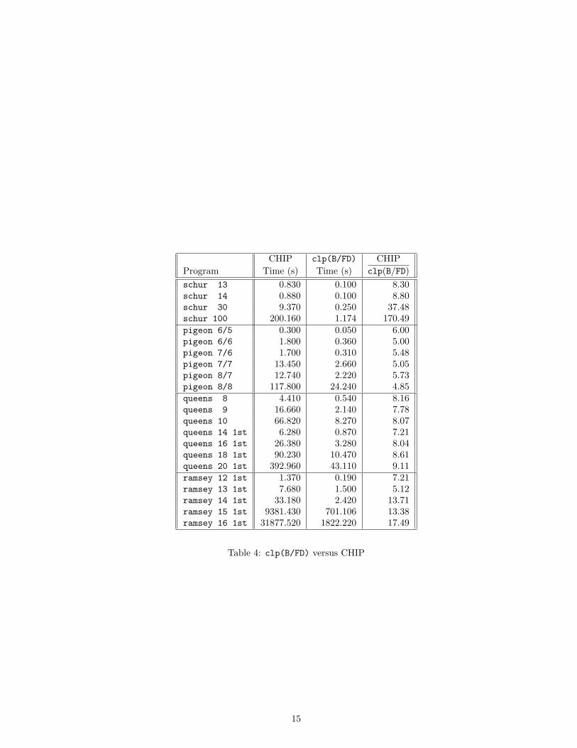
5.3.1 clp(B/FD) versus BDD methods

Adia is an efficient boolean constraint solver based on the use of BDDs. Timemeasurements presented below are taken from [27], in which four different heuristicsare tried on a Sun Sparc IPX (28.5 Mips). We have chosen the worst and the best ofthese four timings for Adia. Note that the BDD approach computes all solutions andis thus unpracticable when we are only interested in one solution for big problemssuch as queens for n ≥ 9 and schur for n = 30. Here again, clp(B/FD) has verygood speedups (see table 5, where the sign ↓ before a number means in fact aslowdown of clp(B/FD) by that factor).

Bdd worst Bdd best clp(B/FD) Bdd worst Bdd bestProgram Time (s) Time (s) Time (s) clp(B/FD) clp(B/FD)schur 13 3.260 1.110 0.100 32.60 11.10schur 14 5.050 1.430 0.100 50.50 14.30pigeon 7/6 1.210 0.110 0.310 3.90 ↓ 2.81pigeon 7/7 3.030 0.250 2.660 1.13 ↓ 10.64pigeon 8/7 4.550 0.310 2.220 2.04 ↓ 7.16pigeon 8/8 15.500 0.580 24.240 ↓ 1.56 ↓ 41.79queens 6 2.410 1.010 0.060 40.16 16.83queens 7 12.030 4.550 0.170 70.76 26.76queens 8 59.210 53.750 0.490 120.83 109.69

Table 5: clp(B/FD) versus a BDD method

5.3.2 clp(B/FD) versus enumerative methods

[26] provides time measurements for an enumerative method for boolean unificationon a Sun 3/80 (1.5 Mips). We normalized these measurements by a factor of 1/19.The average speedup is 6.5 (see table 6).

Enum clp(B/FD) EnumProgram Time (s) Time (s) clp(B/FD)schur 13 0.810 0.100 8.10schur 14 0.880 0.100 8.80pigeon 5/5 0.210 0.060 3.50pigeon 6/5 0.120 0.050 2.40pigeon 6/6 2.290 0.360 6.36pigeon 7/6 0.840 0.310 2.70queens 7 0.370 0.170 2.17queens 8 1.440 0.540 2.66queens 9 6.900 2.140 3.22

Table 6: clp(B/FD) versus an enumerative method

16

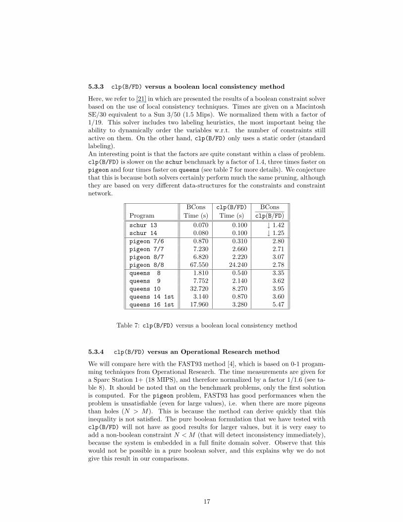
5.3.3 clp(B/FD) versus a boolean local consistency method

Here, we refer to [21] in which are presented the results of a boolean constraint solverbased on the use of local consistency techniques. Times are given on a MacintoshSE/30 equivalent to a Sun 3/50 (1.5 Mips). We normalized them with a factor of1/19. This solver includes two labeling heuristics, the most important being theability to dynamically order the variables w.r.t. the number of constraints stillactive on them. On the other hand, clp(B/FD) only uses a static order (standardlabeling).An interesting point is that the factors are quite constant within a class of problem.clp(B/FD) is slower on the schur benchmark by a factor of 1.4, three times faster onpigeon and four times faster on queens (see table 7 for more details). We conjecturethat this is because both solvers certainly perform much the same pruning, althoughthey are based on very different data-structures for the constraints and constraintnetwork.

BCons clp(B/FD) BConsProgram Time (s) Time (s) clp(B/FD)schur 13 0.070 0.100 ↓ 1.42schur 14 0.080 0.100 ↓ 1.25pigeon 7/6 0.870 0.310 2.80pigeon 7/7 7.230 2.660 2.71pigeon 8/7 6.820 2.220 3.07pigeon 8/8 67.550 24.240 2.78queens 8 1.810 0.540 3.35queens 9 7.752 2.140 3.62queens 10 32.720 8.270 3.95queens 14 1st 3.140 0.870 3.60queens 16 1st 17.960 3.280 5.47

Table 7: clp(B/FD) versus a boolean local consistency method

5.3.4 clp(B/FD) versus an Operational Research method

We will compare here with the FAST93 method [4], which is based on 0-1 progam-ming techniques from Operational Research. The time measurements are given fora Sparc Station 1+ (18 MIPS), and therefore normalized by a factor 1/1.6 (see ta-ble 8). It should be noted that on the benchmark problems, only the first solutionis computed. For the pigeon problem, FAST93 has good performances when theproblem is unsatisfiable (even for large values), i.e. when there are more pigeonsthan holes (N > M). This is because the method can derive quickly that thisinequality is not satisfied. The pure boolean formulation that we have tested withclp(B/FD) will not have as good results for larger values, but it is very easy toadd a non-boolean constraint N < M (that will detect inconsistency immediately),because the system is embedded in a full finite domain solver. Observe that thiswould not be possible in a pure boolean solver, and this explains why we do notgive this result in our comparisons.

17

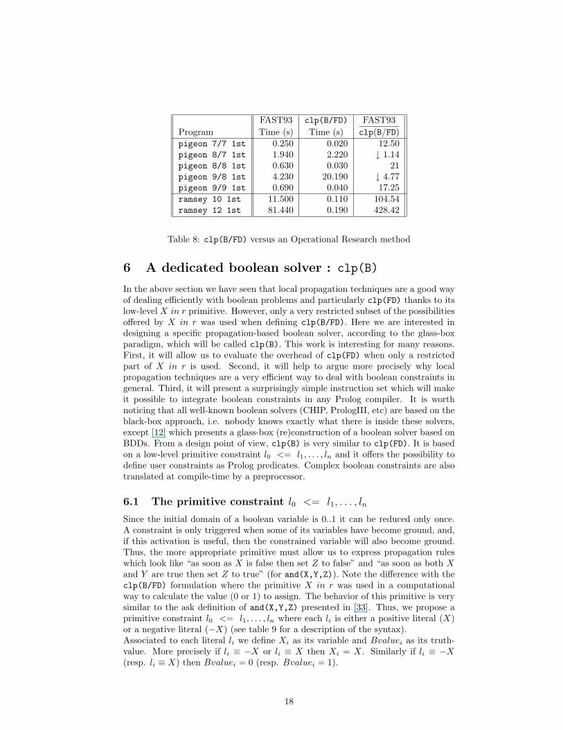
FAST93 clp(B/FD) FAST93Program Time (s) Time (s) clp(B/FD)pigeon 7/7 1st 0.250 0.020 12.50pigeon 8/7 1st 1.940 2.220 ↓ 1.14pigeon 8/8 1st 0.630 0.030 21pigeon 9/8 1st 4.230 20.190 ↓ 4.77pigeon 9/9 1st 0.690 0.040 17.25ramsey 10 1st 11.500 0.110 104.54ramsey 12 1st 81.440 0.190 428.42

Table 8: clp(B/FD) versus an Operational Research method

6 A dedicated boolean solver : clp(B)

In the above section we have seen that local propagation techniques are a good wayof dealing efficiently with boolean problems and particularly clp(FD) thanks to itslow-level X in r primitive. However, only a very restricted subset of the possibilitiesoffered by X in r was used when defining clp(B/FD). Here we are interested indesigning a specific propagation-based boolean solver, according to the glass-boxparadigm, which will be called clp(B). This work is interesting for many reasons.First, it will allow us to evaluate the overhead of clp(FD) when only a restrictedpart of X in r is used. Second, it will help to argue more precisely why localpropagation techniques are a very efficient way to deal with boolean constraints ingeneral. Third, it will present a surprisingly simple instruction set which will makeit possible to integrate boolean constraints in any Prolog compiler. It is worthnoticing that all well-known boolean solvers (CHIP, PrologIII, etc) are based on theblack-box approach, i.e. nobody knows exactly what there is inside these solvers,except [12] which presents a glass-box (re)construction of a boolean solver based onBDDs. From a design point of view, clp(B) is very similar to clp(FD). It is basedon a low-level primitive constraint l0 <= l1, . . . , ln and it offers the possibility todefine user constraints as Prolog predicates. Complex boolean constraints are alsotranslated at compile-time by a preprocessor.

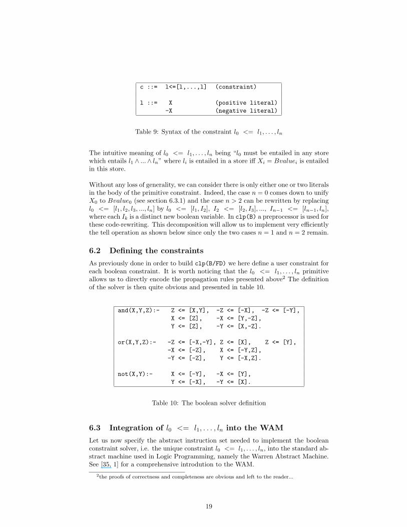
6.1 The primitive constraint l0 <= l1, . . . , ln

Since the initial domain of a boolean variable is 0..1 it can be reduced only once.A constraint is only triggered when some of its variables have become ground, and,if this activation is useful, then the constrained variable will also become ground.Thus, the more appropriate primitive must allow us to express propagation ruleswhich look like “as soon as X is false then set Z to false” and “as soon as both Xand Y are true then set Z to true” (for and(X,Y,Z)). Note the difference with theclp(B/FD) formulation where the primitive X in r was used in a computationalway to calculate the value (0 or 1) to assign. The behavior of this primitive is verysimilar to the ask definition of and(X,Y,Z) presented in [33]. Thus, we propose aprimitive constraint l0 <= l1, . . . , ln where each li is either a positive literal (X)or a negative literal (−X) (see table 9 for a description of the syntax).Associated to each literal li we define Xi as its variable and Bvaluei as its truth-value. More precisely if li ≡ −X or li ≡ X then Xi = X. Similarly if li ≡ −X(resp. li ≡ X) then Bvaluei = 0 (resp. Bvaluei = 1).

18

c ::= l<=[l,...,l] (constraint)

l ::= X (positive literal)-X (negative literal)

Table 9: Syntax of the constraint l0 <= l1, . . . , ln

The intuitive meaning of l0 <= l1, . . . , ln being “l0 must be entailed in any storewhich entails l1 ∧ ...∧ ln” where li is entailed in a store iff Xi = Bvaluei is entailedin this store.

Without any loss of generality, we can consider there is only either one or two literalsin the body of the primitive constraint. Indeed, the case n = 0 comes down to unifyX0 to Bvalue0 (see section 6.3.1) and the case n > 2 can be rewritten by replacingl0 <= [l1, l2, l3, ..., ln] by l0 <= [l1, I2], I2 <= [l2, I3], ..., In−1 <= [ln−1, ln],where each Ik is a distinct new boolean variable. In clp(B) a preprocessor is used forthese code-rewriting. This decomposition will allow us to implement very efficientlythe tell operation as shown below since only the two cases n = 1 and n = 2 remain.

6.2 Defining the constraints

As previously done in order to build clp(B/FD) we here define a user constraint foreach boolean constraint. It is worth noticing that the l0 <= l1, . . . , ln primitiveallows us to directly encode the propagation rules presented above2 The definitionof the solver is then quite obvious and presented in table 10.

and(X,Y,Z):- Z <= [X,Y], -Z <= [-X], -Z <= [-Y],X <= [Z], -X <= [Y,-Z],Y <= [Z], -Y <= [X,-Z].

or(X,Y,Z):- -Z <= [-X,-Y], Z <= [X], Z <= [Y],-X <= [-Z], X <= [-Y,Z],-Y <= [-Z], Y <= [-X,Z].

not(X,Y):- X <= [-Y], -X <= [Y],Y <= [-X], -Y <= [X].

Table 10: The boolean solver definition

6.3 Integration of l0 <= l1, . . . , ln into the WAM

Let us now specify the abstract instruction set needed to implement the booleanconstraint solver, i.e. the unique constraint l0 <= l1, . . . , ln, into the standard ab-stract machine used in Logic Programming, namely the Warren Abstract Machine.See [35, 1] for a comprehensive introdution to the WAM.

2the proofs of correctness and completeness are obvious and left to the reader...

19

6.3.1 Modifying the WAM for boolean variables

Here, we explain the necessary modifications of the WAM to manage a new datatype: boolean variables. They will be located in the heap, and an appropriatetag is introduced to distinguish them from Prolog variables. Dealing with booleanvariables slightly affects data manipulation, unification, indexing and trailing in-structions.

Data manipulation. Boolean variables, as standard WAM unbound variables,cannot be duplicated (unlike it is done for terms by structure-copy). For example,loading an unbound variable into a register consists of creating a binding to thevariable whereas loading a constant consists of really copying it. In the standardWAM, thanks to self-reference representation for unbound variables, the same copyinstruction can be used for both of these kinds of loading. Obviously, a booleanvariable cannot be represented by a self-reference, so we must take care of thisproblem. When a source word Ws must be loaded into a destination word Wd, ifWs is a boolean variable then Wd is bound to Ws or else Ws is physically copiedinto Wd.

Unification. A boolean variable X can be unified with:

• an unbound variable Y : Y is just bound to X,

• an integer n: if n = 0 or n = 1 the pair (X, n) is enqueued and the consistencyprocedure is called (see sections 6.3.3 and 6.3.4).

• another boolean variable Y : equivalent to X <= [Y ], −X <= [−Y ],Y <= [X] and −Y <= [−X]3.

Indexing. The simplest way to manage a boolean variable is to consider it as anordinary unbound variable and thus try all clauses.

Trailing In the WAM, unbound variables only need one word (whose value is fullydefined by their address thanks to self-references), and can only be bound once, thustrailed at most once. When a boolean variable is reduced (to an integer n = 0/1)the tagged word <BLV, > (see section 6.3.2) is replaced by <INT, n> and the taggedword <BLV, > may have to be trailed. So a value-trail is necessary. Hence we havetwo types of objects in the trail: one-word entry for standard Prolog variables,two-word entry for trailing one previous value.

6.3.2 Data structures for constraints

clp(B) uses an explicit queue to achieve the propagation (i.e. each triggered con-straint is enqueued). It is also possible to use an implicit propagation queue asdiscussed in [10]. The register BP (Base Pointer) points to the next constraint toexecute, the register TP (Top Pointer) points to the next free cell in the queue. Theother data structure concerns the boolean variable. The frame of a boolean variableX is shown in table 11 and consists of:

• the tagged word,3we will describe later how constraints are managed.

20

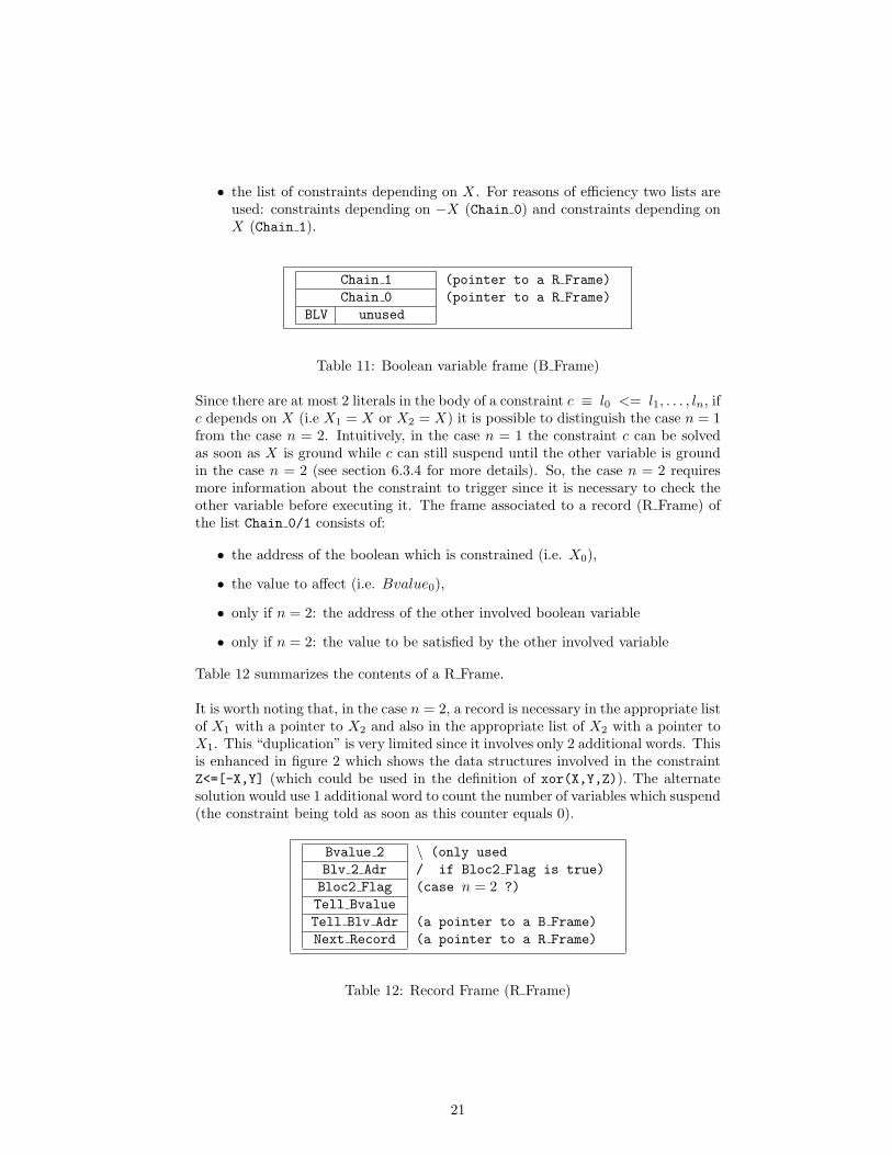
• the list of constraints depending on X. For reasons of efficiency two lists areused: constraints depending on −X (Chain 0) and constraints depending onX (Chain 1).

Chain 1 (pointer to a R Frame)Chain 0 (pointer to a R Frame)

BLV unused

Table 11: Boolean variable frame (B Frame)

Since there are at most 2 literals in the body of a constraint c ≡ l0 <= l1, . . . , ln, ifc depends on X (i.e X1 = X or X2 = X) it is possible to distinguish the case n = 1from the case n = 2. Intuitively, in the case n = 1 the constraint c can be solvedas soon as X is ground while c can still suspend until the other variable is groundin the case n = 2 (see section 6.3.4 for more details). So, the case n = 2 requiresmore information about the constraint to trigger since it is necessary to check theother variable before executing it. The frame associated to a record (R Frame) ofthe list Chain 0/1 consists of:

• the address of the boolean which is constrained (i.e. X0),

• the value to affect (i.e. Bvalue0),

• only if n = 2: the address of the other involved boolean variable

• only if n = 2: the value to be satisfied by the other involved variable

Table 12 summarizes the contents of a R Frame.

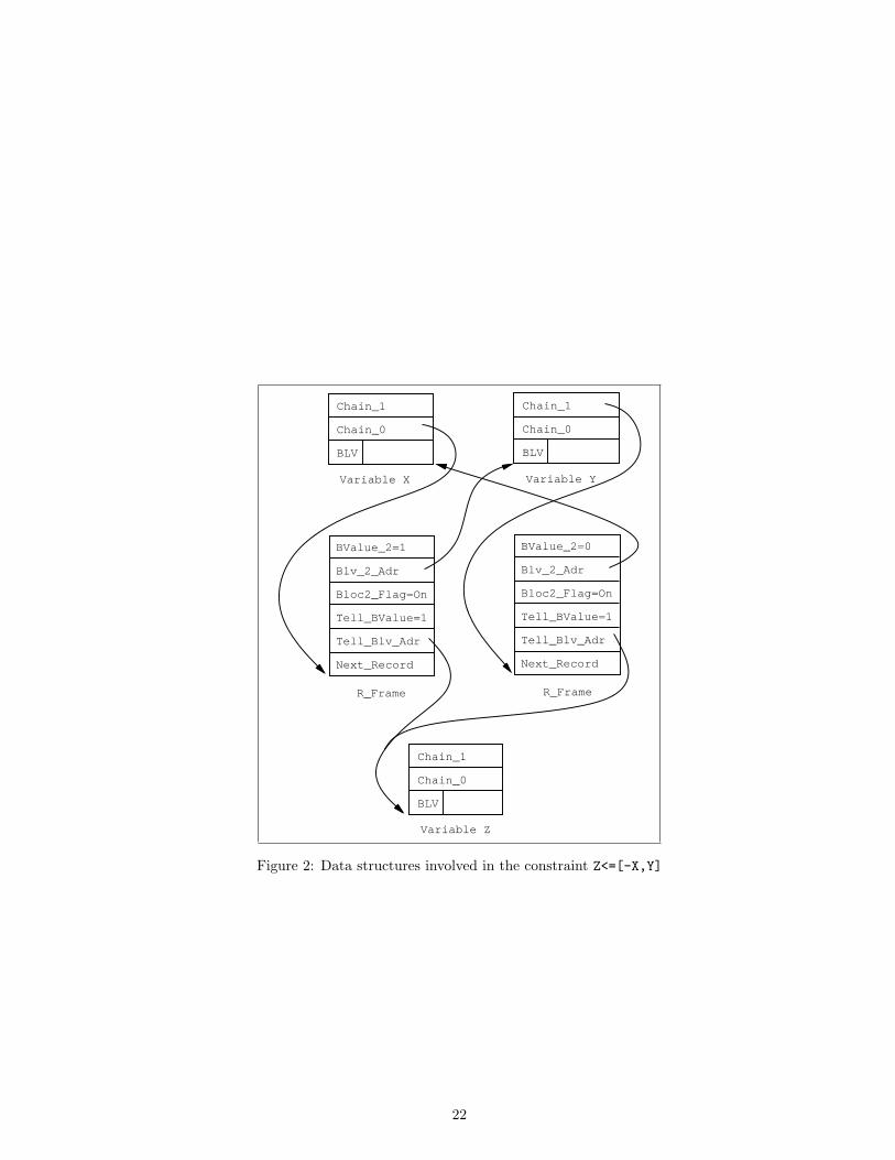
It is worth noting that, in the case n = 2, a record is necessary in the appropriate listof X1 with a pointer to X2 and also in the appropriate list of X2 with a pointer toX1. This “duplication” is very limited since it involves only 2 additional words. Thisis enhanced in figure 2 which shows the data structures involved in the constraintZ<=[-X,Y] (which could be used in the definition of xor(X,Y,Z)). The alternatesolution would use 1 additional word to count the number of variables which suspend(the constraint being told as soon as this counter equals 0).

Bvalue 2 \ (only usedBlv 2 Adr / if Bloc2 Flag is true)Bloc2 Flag (case n = 2 ?)Tell BvalueTell Blv Adr (a pointer to a B Frame)Next Record (a pointer to a R Frame)

Table 12: Record Frame (R Frame)

21

Variable X

Chain_1

Chain_0

BLV

Chain_1

Chain_0

BLV

Chain_1

Chain_0

BLV

Variable Y

Variable Z

BValue_2=1

Blv_2_Adr

Bloc2_Flag=On

Tell_BValue=1

Tell_Blv_Adr

Next_Record

BValue_2=0

Blv_2_Adr

Bloc2_Flag=On

Tell_BValue=1

Tell_Blv_Adr

Next_Record

R_Frame R_Frame

Figure 2: Data structures involved in the constraint Z<=[-X,Y]

22

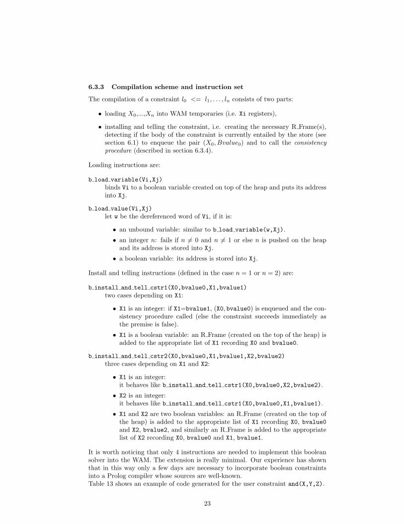
6.3.3 Compilation scheme and instruction set

The compilation of a constraint l0 <= l1, . . . , ln consists of two parts:

• loading X0,...,Xn into WAM temporaries (i.e. Xi registers),

• installing and telling the constraint, i.e. creating the necessary R Frame(s),detecting if the body of the constraint is currently entailed by the store (seesection 6.1) to enqueue the pair (X0, Bvalue0) and to call the consistencyprocedure (described in section 6.3.4).

Loading instructions are:

b load variable(Vi,Xj)binds Vi to a boolean variable created on top of the heap and puts its addressinto Xj.

b load value(Vi,Xj)let w be the dereferenced word of Vi, if it is:

• an unbound variable: similar to b load variable(w,Xj).

• an integer n: fails if n 6= 0 and n 6= 1 or else n is pushed on the heapand its address is stored into Xj.

• a boolean variable: its address is stored into Xj.

Install and telling instructions (defined in the case n = 1 or n = 2) are:

b install and tell cstr1(X0,bvalue0,X1,bvalue1)two cases depending on X1:

• X1 is an integer: if X1=bvalue1, (X0, bvalue0) is enqueued and the con-sistency procedure called (else the constraint succeeds immediately asthe premise is false).

• X1 is a boolean variable: an R Frame (created on the top of the heap) isadded to the appropriate list of X1 recording X0 and bvalue0.

b install and tell cstr2(X0,bvalue0,X1,bvalue1,X2,bvalue2)three cases depending on X1 and X2:

• X1 is an integer:it behaves like b install and tell cstr1(X0,bvalue0,X2,bvalue2).

• X2 is an integer:it behaves like b install and tell cstr1(X0,bvalue0,X1,bvalue1).

• X1 and X2 are two boolean variables: an R Frame (created on the top ofthe heap) is added to the appropriate list of X1 recording X0, bvalue0and X2, bvalue2, and similarly an R Frame is added to the appropriatelist of X2 recording X0, bvalue0 and X1, bvalue1.

It is worth noticing that only 4 instructions are needed to implement this booleansolver into the WAM. The extension is really minimal. Our experience has shownthat in this way only a few days are necessary to incorporate boolean constraintsinto a Prolog compiler whose sources are well-known.Table 13 shows an example of code generated for the user constraint and(X,Y,Z).

23

and/3: b load value(X[0],X[0]) X(0)=address of Xb load value(X[1],X[1]) X(1)=address of Yb load value(X[2],X[2]) X(2)=address of Zb install and tell cstr2(X[2],1,X[0],1,X[1],1) Z <= [X,Y]b install and tell cstr1(X[2],0,X[0],0) -Z <= [-X]b install and tell cstr1(X[2],0,X[1],0) -Z <= [-Y]b install and tell cstr1(X[0],1,X[2],1) X <= [Z]b install and tell cstr2(X[0],0,X[1],1,X[2],0) -X <= [Y,-Z]b install and tell cstr1(X[1],1,X[2],1) Y <= [Z]b install and tell cstr2(X[1],0,X[0],1,X[2],0) -Y <= [X,-Z]proceed Prolog return

Table 13: Code generated for and(X,Y,Z)

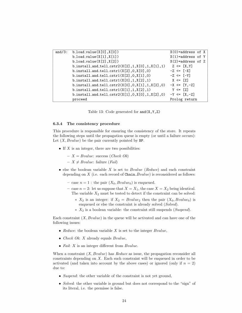
6.3.4 The consistency procedure

This procedure is responsible for ensuring the consistency of the store. It repeatsthe following steps until the propagation queue is empty (or until a failure occurs):Let (X, Bvalue) be the pair currently pointed by BP.

• If X is an integer, there are two possibilities:

– X = Bvalue: success (Check Ok)

– X 6= Bvalue: failure (Fail)

• else the boolean variable X is set to Bvalue (Reduce) and each constraintdepending on X (i.e. each record of Chain Bvalue) is reconsidered as follows:

– case n = 1 : the pair (X0, Bvalue0) is enqueued.

– case n = 2: let us suppose that X = X1, the case X = X2 being identical.The variable X2 must be tested to detect if the constraint can be solved:

∗ X2 is an integer: if X2 = Bvalue2 then the pair (X0, Bvalue0) isenqueued or else the constraint is already solved (Solved).

∗ X2 is a boolean variable: the constraint still suspends (Suspend).

Each constraint (X, Bvalue) in the queue will be activated and can have one of thefollowing issues:

• Reduce: the boolean variable X is set to the integer Bvalue,

• Check Ok: X already equals Bvalue,

• Fail: X is an integer different from Bvalue.

When a constraint (X, Bvalue) has Reduce as issue, the propagation reconsider allconstraints depending on X. Each such constraint will be enqueued in order to beactivated (and taken into account by the above cases) or ignored (only if n = 2)due to:

• Suspend: the other variable of the constraint is not yet ground,

• Solved: the other variable is ground but does not correspond to the “sign” ofits literal, i.e. the premisse is false.

24

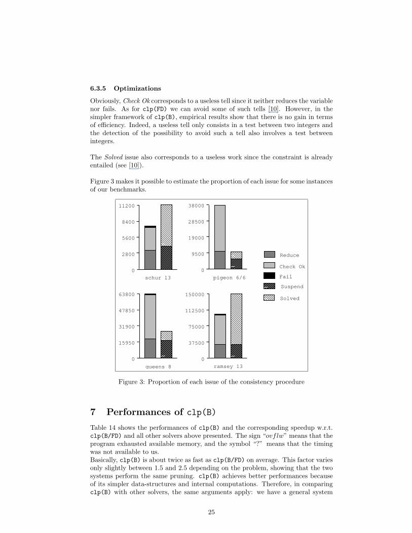
6.3.5 Optimizations

Obviously, Check Ok corresponds to a useless tell since it neither reduces the variablenor fails. As for clp(FD) we can avoid some of such tells [10]. However, in thesimpler framework of clp(B), empirical results show that there is no gain in termsof efficiency. Indeed, a useless tell only consists in a test between two integers andthe detection of the possibility to avoid such a tell also involves a test betweenintegers.

The Solved issue also corresponds to a useless work since the constraint is alreadyentailed (see [10]).

Figure 3 makes it possible to estimate the proportion of each issue for some instancesof our benchmarks.

11200

8400

5600

2800

0

schur 13

38000

28500

19000

9500

0

pigeon 6/6

63800

47850

31900

15950

0

queens 8 ramsey 13

150000

112500

75000

37500

0

Reduce

Check Ok

Fail

Suspend

Solved

Figure 3: Proportion of each issue of the consistency procedure

7 Performances of clp(B)

Table 14 shows the performances of clp(B) and the corresponding speedup w.r.t.clp(B/FD) and all other solvers above presented. The sign “ovflw” means that theprogram exhausted available memory, and the symbol “?” means that the timingwas not available to us.Basically, clp(B) is about twice as fast as clp(B/FD) on average. This factor variesonly slightly between 1.5 and 2.5 depending on the problem, showing that the twosystems perform the same pruning. clp(B) achieves better performances becauseof its simpler data-structures and internal computations. Therefore, in comparingclp(B) with other solvers, the same arguments apply: we have a general system

25

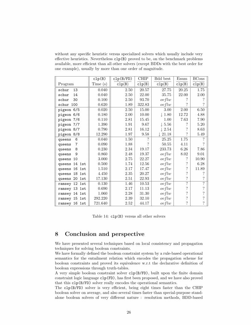
without any specific heuristic versus specialized solvers which usually include veryeffective heuristics. Nevertheless clp(B) proved to be, on the benchmark problemsavailable, more efficient than all other solvers (except BDDs with the best order forone example), usually by more than one order of magnitude.

clp(B) clp(B/FD) CHIP Bdd best Enum BConsProgram Time (s) clp(B) clp(B) clp(B) clp(B) clp(B)schur 13 0.040 2.50 20.57 27.75 20.25 1.75schur 14 0.040 2.50 22.00 35.75 22.00 2.00schur 30 0.100 2.50 93.70 ovflw ? ?schur 100 0.620 1.89 322.83 ovflw ? ?pigeon 6/5 0.020 2.50 15.00 3.00 2.00 6.50pigeon 6/6 0.180 2.00 10.00 ↓ 1.80 12.72 4.88pigeon 7/6 0.110 2.81 15.45 1.00 7.63 7.90pigeon 7/7 1.390 1.91 9.67 ↓ 5.56 ? 5.20pigeon 8/7 0.790 2.81 16.12 ↓ 2.54 ? 8.63pigeon 8/8 12.290 1.97 9.58 ↓ 21.18 ? 5.49queens 6 0.040 1.50 ? 25.25 1.75 ?queens 7 0.090 1.88 ? 50.55 4.11 ?queens 8 0.230 2.34 19.17 233.73 6.26 7.86queens 9 0.860 2.48 19.37 ovflw 8.02 9.01queens 10 3.000 2.75 22.27 ovflw ? 10.90queens 14 1st 0.500 1.74 12.56 ovflw ? 6.28queens 16 1st 1.510 2.17 17.47 ovflw ? 11.89queens 18 1st 4.450 2.35 20.27 ovflw ? ?queens 20 1st 17.130 2.51 22.93 ovflw ? ?ramsey 12 1st 0.130 1.46 10.53 ovflw ? ?ramsey 13 1st 0.690 2.17 11.13 ovflw ? ?ramsey 14 1st 1.060 2.28 31.30 ovflw ? ?ramsey 15 1st 292.220 2.39 32.10 ovflw ? ?ramsey 16 1st 721.640 2.52 44.17 ovflw ? ?

Table 14: clp(B) versus all other solvers

8 Conclusion and perspective

We have presented several techniques based on local consistency and propagationtechniques for solving boolean constraints.We have formally defined the boolean constraint system by a rule-based operationalsemantics for the entailment relation which encodes the propagation scheme forboolean constraints and proved its equivalence w.r.t the declarative definition ofboolean expressions through truth-tables.A very simple boolean constraint solver clp(B/FD), built upon the finite domainconstraint logic language clp(FD), has first been proposed, and we have also provedthat this clp(B/FD) solver really encodes the operational semantics.The clp(B/FD) solver is very efficient, being eight times faster than the CHIPboolean solver on average, and also several times faster than special-purpose stand-alone boolean solvers of very different nature : resolution methods, BDD-based

26

methods, enumerative methods, Operational Research techniques. This provesfirstly that the propagation techniques proposed for finite domains are very com-petitive for booleans and secondly that, among such solvers, the glass-box approachof using a single primitive constraint X in r is very interesting and it makes itpossible to encode other domains (such as boolean domains) at a low-level, withbetter performances than the “black-box”. An additional advantage is the completeexplicitation of the propagation scheme.Nevertheless, performances can be improved by simplifying the data-structures usedin clp(FD), which are designed for full finite domain constraints, and specializingthem for booleans by explicitly introducing a new type and new instructions forboolean variables. For instance, it is possible to reduce the variable frame repre-senting the domain of a variable and its associated constraints to only two words:one pointing to the chain of constraints to awake when the variable is bound to 0and the other when it is bound to 1. Such a solver is very compact and simple; it isbased again on the glass-box approach, and uses only a single low-level constraint,more specialized than the X in r construct, into which boolean constraints suchas and, or or not are decomposed. This primitive constraint can be implementedin a WAM-based logical engine with a minimal extension : only four new abstractinstructions are needed. This surprisingly simple instruction set makes it possibleto integrate boolean constraints in any Prolog compiler very easily. Our experi-ence shows that it only requires a few days of implementation work... Moreover,this dedicated solver, called clp(B), provides a further factor two speedup w.r.t.clp(B/FD) and is therefore more efficient than all other solvers we have been ableto compare with.It is worth noticing that in clp(FD) the only heuristic available for labeling is theclassical “first-fail” based on the size of the domains which is obviously useless forboolean constraints. Some more flexible primitives (e.g. number of constraints onX, number of constraints using X) would be necessary in order to express, at thelanguage level, some complex labeling heuristics [31], [21]. Such a labeling howeverrequires complex entailment and disentailment detection for constraint, that we arecurrently investigating [9].

27

References

[1] H. Aıt-Kaci. Warren’s Abstract Machine, A Tutorial Reconstruction. LogicProgramming Series, MIT Press, Cambridge, MA, 1991.

[2] F. Benhamou. Boolean Algortihms in PrologIII. In Constraint Logic Program-ming: Selected Research, A. Colmerauer and F. Benhamou (Eds.). The MITPress, 1993.

[3] H. Bennaceur and G. Plateau. FASTLI: An Exact Algorithm for the Con-straint Satisfaction Problem: Application to Logical Inference. Research Re-port, LIPN, Universite Paris-Nord, Paris, France, 1991.

[4] H. Bennaceur and G. Plateau. Logical Inference Problem in Variables 0/1. inIFORS 93 Conference, Lisboa, Portugal, 1993.

[5] BNR-Prolog User’s Manual. Bell Northern Research. Ottawa, Canada, 1988.

[6] A. Bockmayr. Logic Programming with Pseudo-Boolean Constraints. Researchreport MPI-I-91-227, Max Planck Institut, Saarbrucken, Germany, 1991.

[7] R.E. Bryant, Graph Based Algorithms for Boolean Fonction Manipulation.IEEE Transactions on computers, no. 35 (8), 1986, pp 677–691.

[8] W. Buttner and H. Simonis. Embedding Boolean Expressions into Logic Pro-gramming. Journal of Symbolic Computation, no. 4 (1987), pp 191-205.

[9] B. Carlsson, M. Carlsson, D. Diaz Entailment of Finite Domain Constraints.draft, 1993.

[10] P. Codognet and D. Diaz. Compiling Constraint in clp(FD). draft, 1993.

[11] A. Colmerauer. An introduction to PrologIII. Communications of the ACM,no. 28 (4), 1990, pp 412-418.

[12] M. M. Corsini and A. Rauzy. CLP(B): Do it yourself. In GULP’93, ItalianConference on Logic Programming, Gizzeria Lido, Italy, 1993.

[13] D. Diaz and P. Codognet. A Minimal Extension of the WAM for clp(FD).In 10th International Conference on Logic Programming, Budapest, Hungary,The MIT Press 1993.

[14] G. Dore and P. Codognet. A Prototype Compiler for Prolog with BooleanConstraints. In GULP’93, Italian Conference on Logic Programming, GizzeriaLido, Italy, 1993.

[15] G. Gallo, G. Urbani, Algorithms for Testing the Satisfiability of PropositionalFormulae. Journal of Logic Programming, no. 7 (1989), pp 45-61.

[16] R. M. Haralick and G. L. Elliot. Increasing Tree Search Efficiency for ConstraintSatisfaction Problems. Artificial Intelligence 14 (1980), pp 263-313

[17] J. N. Hooker and C. Fedjki. Branch-and-Cut Solution of Inference Problemsin Propositional Logic. Research Report, Carnegie-Mellon University Pittsurh,Pennsylvania, 1987.

28

[18] J. Jaffar and J-L. Lassez. Constraint Logic Programming. In Principles OfProgramming Languages, Munich, Germany, January 1987.

[19] A. K. Mackworth. Consistency in Networks of Relations. Artificial Intelligence8 (1977), pp 99-118.

[20] U. Martin, T. Nipkow, Boolean Unification – The story so far. Journal ofSymbolic Computation, no. 7 (1989), pp 191-205.

[21] J-L. Massat. Using Local Consistency Techniques to Solve Boolean Con-straints. In Constraint Logic Programming: Selected Research, A. Colmerauerand F. Benhamou (Eds.). The MIT Press, 1993.

[22] U. Montanari. Networks of constraints: Fundamental properties and applica-tion to picture processing. In Information Science, 7 (1974).

[23] B. A. Nadel. Constraint Satisfaction Algorithms. Computational Intelligence5 (1989), pp 188-224.

[24] A. Rauzy. L’Evaluation Semantique en Calcul Propositionnel. PhD thesis,University of Aix-Marseille II, Marseille, France, January 1989.

[25] A. Rauzy. Adia. Technical report, LaBRI, Universite Bordeaux I, 1991.

[26] A. Rauzy. Using Enumerative Methods for Boolean Unification. In Con-straint Logic Programming: Selected Research, A. Colmerauer and F. Ben-hamou (Eds.). The MIT Press, 1993.

[27] A. Rauzy. Some Practical Results on the SAT Problem, Draft, 1993.

[28] V. Saraswat. The Category of Constraint Systems is Cartesian-Closed. In LogicIn Computer Science, IEEE Press 1992.

[29] D. S. Scott Domains for Denotational Semantics. In ICALP’82, InternationalColloquium on Automata Languages and Programmaing, 1982.

[30] H. Simonis, M. Dincbas, “Propositional Calculus Problems in CHIP”, ECRC,Technical Report TR-LP-48, 1990.

[31] P. Van Hentenryck. Constraint Satisfaction in Logic Programming. Logic Pro-gramming Series, The MIT Press, Cambridge, MA, 1989.

[32] P. Van Hentenryck, V. Saraswat and Y. Deville. Constraint Processing incc(FD). Draft, 1991.

[33] P. Van Hentenryck, H. Simonis and M. Dincbas. Constraint Satisfaction UsingConstraint Logic Programming. Artificial Intelligence no 58, pp 113-159, 1992.

[34] P. Van Hentenryck, Y. Deville and C-M. Teng. A Generic Arc-ConsistencyAlgorithm and its Specializations. Artificial Intelligence 57 (1992), pp 291-321.

[35] D. H. D. Warren. An Abstract Prolog Instruction Set. Technical Report 309,SRI International, Oct. 1983.

29